UNCLASSIFIED

Defense Technical Information CenterCompilation Part Notice

ADP012089TITLE: Supercavitating 2-D Hydrofoils: Prediction of Performance andDesign

DISTRIBUTION: Approved for public release, distribution unlimited

This paper is part of the following report:

TITLE: Supercavitating Flows [les Ecoulements supercavitants]

To order the complete compilation report, use: ADA400728

The component part is provided here to allow users access to individually authored sectionsf proceedings, annals, symposia, etc. However, the component should be considered within

[he context of the overall compilation report and not as a stand-alone technical report.

The following component part numbers comprise the compilation report:ADP012072 thru ADP012091

UNCLASSIFIED

21-1

SUPERCAVITATING 2-D HYDROFOILS:PREDICTION OF PERFORMANCE AND DESIGN

Spyros A. Kinnas

Ocean Engineering Group, Department of Civil EngineeringThe University of Texas at Austin, Austin, TX 78712, USAhttp://cavity.ce.utexas. edu, email: kinnasPmaiLutexas. edu

ABSTRACT

Recent numerical techniques for the prediction of cavitating flows, in linear and non-linear theories, are appliedon super-cavitating 2-D, 3-D hydrofoils and propellers. Some of these techniques, when incorporated within anon-linear optimization algorithm, can lead to efficient super-cavitating hydrofoil or propeller designs. Thislecture will address 2-D supercavitating hydrofoils.

1 INTRODUCTIONHigh-speed hydrofoil or propeller applications can benefit considerably, in terms of efficiency, by operating

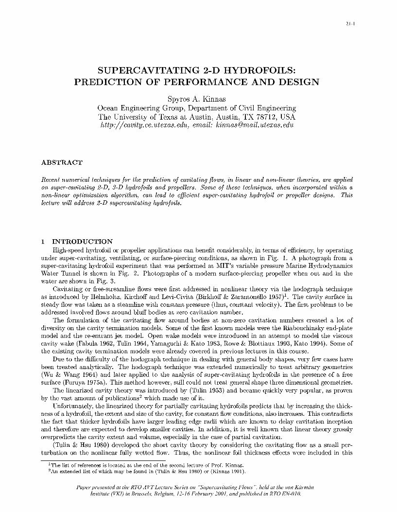
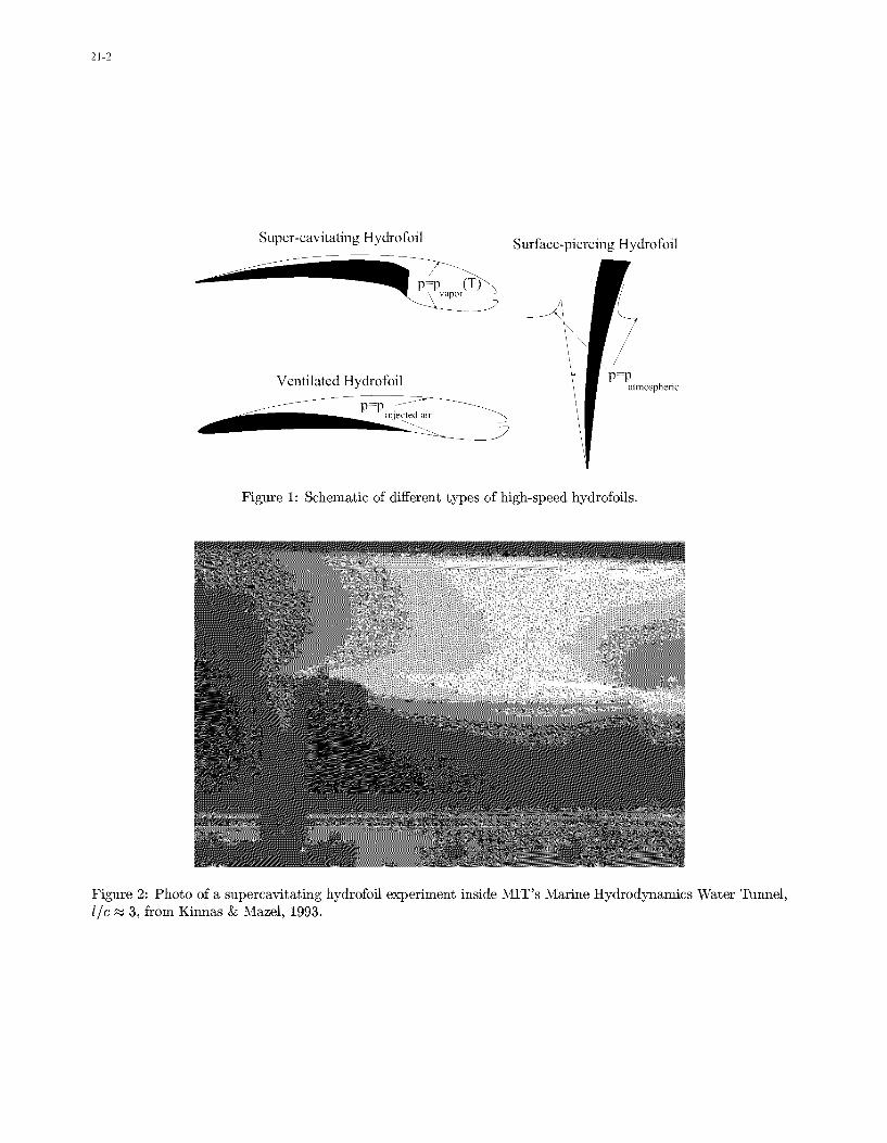
under super-cavitating, ventilating, or surface-piercing conditions, as shown in Fig. 1. A photograph from asuper-cavitating hydrofoil experiment that was performed at MIT's variable pressure Marine HydrodynamicsWater Tunnel is shown in Fig. 2. Photographs of a modern surface-piercing propeller when out and in thewater are shown in Fig. 3.

Cavitating or free-streamline flows were first addressed in nonlinear theory via the hodograph techniqueas introduced by Helmholtz, Kirchoff and Levi-Civita (Birkhoff & Zarantonello 1957)1. The cavity surface insteady flow was taken as a steamline with constant pressure (thus, constant velocity). The first problems to beaddressed involved flows around bluff bodies at zero cavitation number.

The formulation of the cavitating flow around bodies at non-zero cavitation numbers created a lot ofdiversity on the cavity termination models. Some of the first known models were the Riabouchinsky end-platemodel and the re-entrant jet model. Open wake models were introduced in an attempt to model the viscouscavity wake (Fabula 1962, Tulin 1964, Yamaguchi & Kato 1983, Rowe & Blottiaux 1993, Kato 1994). Some ofthe existing cavity termination models were already covered in previous lectures in this course.

Due to the difficulty of the hodograph technique in dealing with general body shapes, very few cases havebeen treated analytically. The hodograph technique was extended numerically to treat arbitrary geometries(Wu & Wang 1964) and later applied to the analysis of super-cavitating hydrofoils in the presence of a freesurface (Furuya 1975a). This method however, still could not treat general shape three dimensional geometries.

The linearized cavity theory was introduced by (Tulin 1953) and became quickly very popular, as provenby the vast amount of publications2 which made use of it.

Unfortunately, the linearized theory for partially cavitating hydrofoils predicts that by increasing the thick-ness of a hydrofoil, the extent and size of the cavity, for constant flow conditions, also increases. This contradictsthe fact that thicker hydrofoils have larger leading edge radii which are known to delay cavitation inceptionand therefore are expected to develop smaller cavities. In addition, it is well known that linear theory grosslyoverpredicts the cavity extent and volume, especially in the case of partial cavitation.

(Tulin & Hsu 1980) developed the short cavity theory by considering the cavitating flow as a small per-turbation on the nonlinear fully wetted flow. Thus, the nonlinear foil thickness effects were included in this

'The list of references is located at the end of the second lecture of Prof. Kinnas.'An extended list of which may be found in (Tulin & llsu 1980) or (Kinnas 1991).

Paper presented at the RTO A VT Lecture Series on "Supercavitating Flows ", held at the von KcirmanInstitute (VKI) in Brussels, Belgium, 12-16 February 2001, and published in RTO EN-O 10.

21-2

Super-cavitating Hydrofoil Surface-piercing Hydrofoil

0'( apr -T)

Ventilated Hydrofoil Ptpatmospheric

Figure 1: Schematic of different types of high-speed hydrofoils.

Figure 2: Photo of a supercavitating hydrofoil experiment inside MIT's Marine Hydrodynamics Water Tunnel,i/c z 3, from Kinnas & Mazel, 1993.

21-3

Figure 3: Photos of a surface-piercing propeller Model 841-B (top), and one of its blades after it has entered thefree-surface, with leading edge detachment at Js = 0.9 (middle), and with midehord detachment at JS = 1.0(bottom). For clarity, the blade has been outlined in the photos. From Olofsson (1996).

21-4

formulation. This method predicted that by increasing the thickness of a partially cavitating hydrofoil, the sizeof the cavity was reduced substantially for fixed flow conditions.

A nonlinear numerical method was employed to analyze cavitating hydrofoils by using surface vorticitytechniques and by applying the exact boundary conditions on the cavity and on the foil (Uhlman 1987, Uhlman1989). An end-plate cavity termination model was implemented. A reduction in the size of the cavity as the foilthickness increased was predicted, but not as drastic as that predicted in (Tulin & Hsu 1980). A surface vorticitytechnique to deal with thick foil sections which employed an open cavity model was developed in (Yamaguchi& Kato 1983). Similar boundary element method techniques were developed by (Lemonnier & Rowe 1988) andby (Rowe & Blottiaux 1993). Potential based boundary element methods were finally applied by (Kinnas &Fine 1991b, Kinnas & Fine 1993) and by (Lee et al 1992).

Three-dimensional flow effects around cavitating finite span hydrofoils were treated first in strip-theory viamatching with an inner two-dimensional solution within either linear (Nishiyama 1970, Leehey 1971, Uhlman1978, Van Houten 1982) or non-linear theory (Furuya 1975b).

The complete three-dimensional super-cavitating hydrofoil problem was first treated in linear theory via anumerical lifting surface approach based on the pressure source and doublet technique (Widnall 1966) and latervia a vortex and source lattice technique (Jiang & Leehey 1977). In the latter work, an iterative scheme wasintroduced which determined the extent of the cavity by requiring the pressure distribution on the cavity to beconstant along the span (in addition to being constant along the chord). A variational approach for determiningthe cavity planform was introduced in (Achkinadze & Fridman 1994).

Numerical boundary element methods within non-linear cavity theory were naturally extended to treatsuper-cavitating 3-D hydrofoils (Pellone & Rowe 1981) and 3-D hydrofoils with partial cavities (Kinnas & Fine1993) or cavities with mixed (partial and super-cavities) planforms (Fine & Kinnas 1993a). Similar methodswere also developed by (Kim et al 1994, Pellone & Peallat 1995).

The first effort to analyze the complete three dimensional unsteady flow around a cavitating propellersubject to a spatially non-uniform inflow was presented in (Lee 1979, Lee 1981, Breslin et al 1982). A sourceand vortex lattice lifting surface scheme was employed and the unsteady three dimensional linearized boundaryconditions were applied on the cavity. The cavity planform was determined at each blade strip and each timestep (i.e., blade angle) by searching for the cavity length which would produce the desired vapor pressure insidethe cavity. The effect of the other strips was accounted for in an iterative sense by "sweeping" along the spanwisedirection of the blade back and forth until the cavity shape converged. Similar methods were presented morerecently by (Ishii 1992, Szantyr 1994, Kudo & Ukon 1994).

Unfortunately, all these 3-D methods are hampered by the inherent inability of linear cavity theory to predictthe correct effect of blade thickness on cavity shape, as already mentioned. This deficiency was corrected in twodimensions in (Kinnas 1985, Kinnas 1991), where the leading edge correction was introduced in the linearizeddynamic boundary condition on the cavity. The leading edge correction was subsequently applied to the threedimensional propeller solution (Kerwin et al 1986, Kinnas 1992b).

Non-linear methods based on an assumed semi-elliptic cavity sectional shape have also been applied (Stern& Vorus 1983) and (Van Gent 1994). Non-linear potential-based boundary element methods were finally appliedto cavitating propellers in non-uniform flows by (Kinnas & Fine 1992, Fine & Kinnas 1993b), and more recentlyby (Kim & Lee 1996).

The inviscid cavity flow method was coupled with a boundary layer solver in the case of partial and super-cavitating 2-D hydrofoils by (Kinnas et al 1994). This allowed for the inclusion of the viscous boundary layerin the wake of the cavity and for determining the cavity detachment point based on the viscous flow upstreamof the cavity.

Reynolds-Averaged Navier-Stokes solvers have also been applied in the case of the prediction of attachedsheet cavitation on 2-D hydrodoils (Kubota et al 1989, Deshpande et al 1993). An overview of viscous flowsolvers applied to cavitating flows may be found in (Kato 1996). However, these methods appear to be bestsuited for the prediction of cloud and or detached cavitation.

In these two lectures, linear and nonlinear methods for the prediction of super-cavitation on hydrofoilsand propellers will be summarized, and some comparisons with experiments will be presented. Non-linearoptimization techniques, applicable to the design of 2-D super-cavitating sections and super-cavitating propellerblades, will be also presented.

21-5

Dynamic Boundary Condition

Cavity Detachment (constant pressure condition) Cavity Closure Condition

L ki

(flow tangency condition)

c

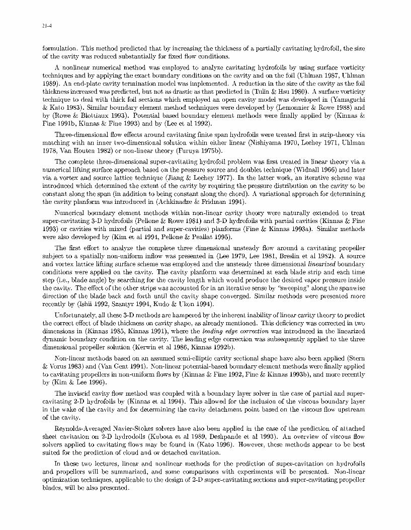
Figure 4: Formulation of the inviscid cavity flow problem

2 2-D HYDROFOIL2.1 Formulation

Consider the 2-D super-cavitating hydrofoil3 , as shown in Fig. 4. Assuming inviscid and irrotational flow,the governing equation everywhere inside the fluid region is given by4:

V2=0 (1)

where 0 is the the perturbation potential defined from:

q = U± + VO (2)

where q is the total velocity vector in the flow. In order to uniquely determine 0, the following boundaryconditions are imposed:

"* On the wetted foil surface, the following kinematic boundary condition is applied, which requires the fluidflow to be tangent to the surface of the foil. Therefore,

On__ 00 --U -n (3)

where n is the surface unit normal vector.

"* At infinity the perturbation velocities should go to zero.

VO -4 0 (4)

"* The dynamic boundary condition specifies constant pressure on the cavity, or (via Bernoulli equation)constant cavity velocity qc:

q, = U00 Tr±+ (5)

where the cavitation number, o, is defined as:

= P- PC (6)

2 '0

pc, is the pressure corresponding to a point in the free-stream and p, is the pressure inside the cavity.3 The application of the methods to partially cavitating hydrofoils is straight-forward and the reader can find more details in

(Kinnas 1998).4 The cavity is assumed to detach at a known location on the foil. A criterion for determining this location will be discussed in

a later section.

21-6

Y ' 'h (X

U " W l) ,TE

tor

Fiue5 Suecvttn hyrfi 'nlna hoy

C= d''

0C dxI u =,72

wlbeadesd in a lae secion

u- (/ UU

veoct, tr ve , trnito rgon dx u c2Uo

V =U(,~dx

, x) (x)x y(ý) dý or q(ý)dý

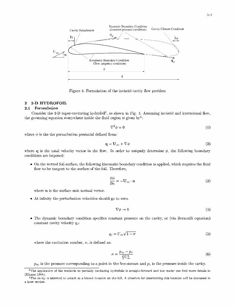
Figure 5: Supercavitating hydrofoil in linear theory.

The following conditions at the trailing edge of the cavity:

1. The cavity closes at its trailing edge. The inclusion of the viscous wake downstream of the cavitywill be addressed in a later section.

2. Near the trailing edge of the cavity, the pressure recovery termination model renders for the cavityvelocity, qt,•, over a transition region Ac:

qtr = U. V/1 -+Ocr [I f W~x] (7)

where f(x) is an algebraic function defined in (Kinnas T Fine 1993).

The problem of finding the cavitation number for given cavity extent, 1, will be addressed first in the contextof linear and nonlinear theories. A method for determining the cavity extent for given cavitation number willbe described in a later section.

2.2 Linear theoriesIn this section, the linearized cavitating hydrofoil problem is formulated in terms of singular integral equa-

tions with respect to unknown vorticity and source distributions. These integral equations are inverted analyt-ically in the case of general shape supercavitating hydrofoils. The cavitation number, the vorticity and sourcedistributions are expressed in terms of integrals of quantities which depend only on the foil geometry and the

cavity length. The procedure is summarized here. The details are given in (Kinnas 1992a) and (Kinnas & Fine1991a).

We define as u and v the perturbation velocities tangent and normal to the direction of the incoming flowrespectively, as shown in Figure 5. In the context of the linearized cavity theory the boundary conditions of thecorresponding Hilbert problem are:

The kinematic boundary conditions:

21-7

v-=U" ; 0<x<1, y=0- (8)~dx

v =U. di. O<X<lD, y=0+ (9)dx

The dynamic boundary conditions:

u+ = -7-Uo; lD<X<l,y=O (10)2

u = £U"O ; l<x<l, y=0- (11)2

where qp (x) and qu(x) are the ordinates of the lower and upper hydrofoil surface, respectively, as shown inFigure 5. These boundary conditions can be expressed in terms of vorticity and source distributions 5 -y(x) andq(x), respectively, located on the slit x E [0, 1].

- q + (12)

+ IJ (13)2 27r•, --X

u- _ I 1 q(Od (14)

By using equations (10), (11), (13), and (14) it can easily be shown that:

'Y(x)=0; 1<x<l (15)

Finally, and with the use of the definitions:

7d q(a x)- q(x) (16)•(x)- aUd• x U•

the complete boundary value problem becomes:

1. Kinematic Boundary Conditions

- - ±( ) d - e-x O x<_= O (

+ f 0*(x) 1 <X < x I < 0 (17)2 271')01

+ f -ý ='9 ;X 0 < X< ID , Y =0 (18)0

2. Dynamic Boundary Condition

f2I <, X: =2 < I , Y = 0+(19)

0

3. Kutta Condition6

7(1) =0 (20)

5 With f designating the Cauchy principal value of the integral.6 The application of a Kutta condition may seem unnecessary due to the requirement of a finite pressure, thus velocity, at the

foil trailing edge. Nevertheless, this condition is still required when inverting the integral equations.

21-8

4. Cavity Closure Condition 7

J/q(x)dx = 0 (21)

0

where

0*=Il and 0* ld (22)1 or dx U or dx

2.2.1 Inversion of the Integral Equations - ID = 0In the case of leading edge detachment (ID = 0), the singular integral equations of Cauchy type, (17) and

(19), can be inverted to produce expressions for the unknown or, 7(x) and q(x) in terms of the cavity length Iand the lower hydrofoil surface qp(x), as follows (Kinnas 1992a):

First, equation (19) is inverted with respect to the unknown q(x) (Muskhelishvili 1946) to produce:

j [:1:XJ' F - ý 7()dý 23

where use of equation (15) has been made. Notice that the expression (23) corresponds to the unique solutionto (19) which behaves like 1/V -- x at the trailing edge of the cavity ( Wu's singularity (Wu 1957) ). Bysubstituting equation (23) in (17) and by using the substitutions:

X=, . = 1 1 (24)

we arrive at the following singular integral equation of Cauchy type for 7:

1f •()d17 z e7(z) S(25)2700 (1 +.q 2 )(z -q) 4(1±+z2) 2(1±+z2)

Inversion of equation (25) with respect to the variable (,)q/(1 + .2) renders finally:

7(z)- (1+ Z2) V t- Z f- V 77) (26)Z V 0 V t (216 )•-7 7 . dTr Z~j t (I1+r7 2)(Z-_,q)dr

Notice that 7(z) in equation (26) is the unique solution to (25) which satisfies the Kutta condition (20) at z = t.The cavitation number or is determined by satisfying the cavity closure condition (21). First, by substituting

equation (23) in (21) and by using equation (15) we can get (Kinnas 1992a):

-7 '+ 7()d = 0, (27)

and by substituting equation (26) we can get the following general expression for or (Kinnas 1992a):

4or V/-2r4 Vj r 2 __±• ,l -- [ d,],- r(r 2 + 1) t (I +,q 2 ) 2 Tx ] dq (28)

where: r = V/T+1t2 .The source distribution can be derived by substituting equation (26) into equation (23) (Kinnas 1992a):

(z) = -t(Z) -+ tz (Vr r--1 - zvr 2 1)

V Z 2V/2r2

I1+ 2 t±+- tf w 0*(w)dcw1-__2tS ft Vt (_ O')Jd (29)

Tjz t- w (1 + W2 )(Z "+- (2)

7We apply the linearized cavity closure condition in which the cavity is required to have zero thickness at its trailing edge. The

present method can be extended to treat open cavities at the trailing edge with the openness of the cavity, possibly supplied fromfurther knowledge of the viscous wake behind the cavity. The effects of viscosity will be addressed at a later section.

21-9

for z < t, and:

( Z) = i -tz (vr - I - zv 2 + 1)z 2v/-r.2

1±+ t2 z f I (w)dT z JO (I + (1W 2)(Z +W)

z-t (zvr-2 ±+ I + vr--)z 2v'2r2

1l+ Z2 [Z--

t ft 0* e (w) dco( 0T V -Z Jo + W-C iJ-C2)(Z -- W) (0

for z > t.

2.2.2 Inversion of the Integral Equations - ID > 0

In this case, as shown in (Kinnas & Fine 1991a), equations (26), (29), and (30) still apply, after the followingsubstitutions are made:

replace 7 with T-2(u+-C ) ; 0<x<lID (31)

and

replace 0* with 0* + F (32)

with

F(x) (33)•-x

where u+ is the horizontal perturbation velocity on the wetted part on the suction side of the foil, divided byuU'o. The value of u+ is determined by applying the kinematic boundary condition on the upper wetted partof the hydrofoil, equation (9). This is equivalent to requiring that the value of q(x) for 0 < x < ID is equalto the value of the thickness source in the case of wetted flow. A rather lengthy formula for u+, as well anexpression for the modified value of a are given in (Kinnas & Fine 1991a), and are not included in this lecture.

2.2.3 The cavity shapeThe cavity thickness h(x), which also includes the foil thickness as shown in Figure 5, is determined, within

the framework of linearized theory, by integrating the equation:

uodh (4U. X = q(x) (34)

The camber of the cavity in the wake, c(x), is determined by integrating the following equation:

dcU.- = vw(x) for 1<x<l (35)

dx

where vw,(x) is the normal perturbation velocity in the wake, given as follows:

1 fl y(1)dý ; l<x<l, y=O (36)

By substituting equation (26) in (36) we can get v, in terms of the hydrofoil geometry (Kinnas & Fine1991a):

21-10

Vw(Z) tz+-z (VP - I -z r 2 ±• )oU• V ~z 4'-•r.2

i1±z2 t±T+-_ zf':¢ e7(w)dw2w vz• o t- (i+w 2 )(z+w)z--t (zr 2 ±i± r 2 -- )

z 4Vr2.2i+ z2 z--f t w 0* (w)dw

27 w fo t- W (I +W 2 )(Z)•( •)

The pressure distribution on the upper and lower cavity or foil surface is given, in the context of lineartheory, as follows:

C1 02rO X<,=+ (38)C1 -2 [xfJ~l; °<x<l, y=0~(8

02 2w_ )-x ; o<x<l,y=O- (39)

where Cp is the pressure coefficient defined as:

CP = P -Poo(0PJCX (40)2 0

2.2.4 Numerical IntegrationsThe integrals in equations (28), (26), (29) and (30) are computed numerically with special care taken at

the singularities of the integrands. We first define the transformation:

77=t sin2(') ; 0< _<•tand0<0<7r (41)

Next, we expess the involved integrals in terms of 0, thus avoiding the square root singularities of theintegrands at 7 = 0 and 77 = t. The numerical integrations are then performed by applying Simpson's rule withK uniform intervals in 0.

To compute the principal value of the singular integral in equation (26), we first factor out the involvedsingularity as follows (Kinnas 1992a):

___rt f(rj) d, f f()_f(z) (4

__ _ djw )(42)wher t~q f (z)J. 7"(Ztzr, 7 0 V ~ Z-T)

where f (,q) 9 ( Notice that the integrand in the integral of equation (42) is not singular anymore, andthus the integral is computed numerically by applying the same methodology described in the beginning of thissection. As shown in (Kinnas 1992a), Simpson's rule produces very accurate values for the integrals even withfive uniform intervals (K = 5).

2.2.5 The vortex/source-lattice methodA direct numerical method must be applied in the case of 3-D hydrofoils or propeller blades, as in (Lee

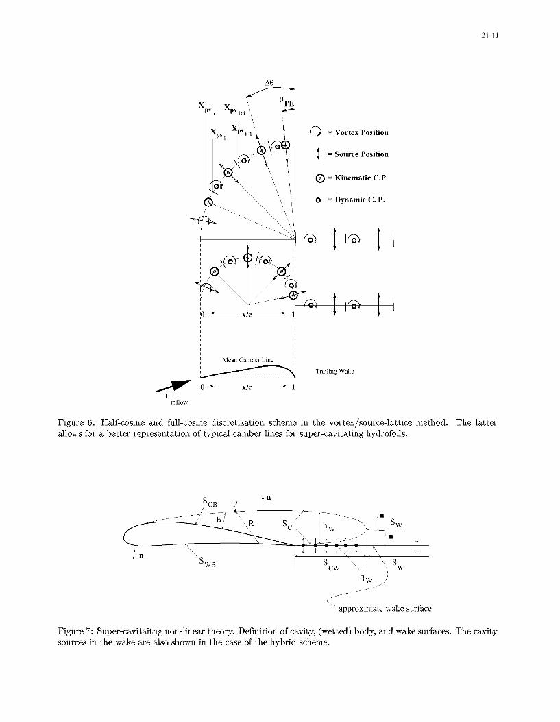
1979, Kinnas et al 1998a, Kosal 1999). In this case the involved integrals are disretized first, then the boundaryconditions are applied at some appropriately selected control points (C.P.s), and finally, the resulting systemof linear equations is inverted. The integrals in equations (17) and (19) are disretized over each segment iby replacing -(•)dý with -yi(Xpv,+l - Xpv,), and q(ý)dý with qi(Xpsi+l - Xps•). Figure 6 shows two types ofarrangements for the discrete vortices and sources and the correpsonding control points.

21-11

Ae

, 0 TE l• P s i+ l/ I ll •(

x , = Vortex Position

= Source Position

o = Kinematic C.P.

0 =Dynamic C. P.

\r

Mean Camber Line

Trailing Wake

Uinflow

Figure 6: Half-cosine and full-cosine discretization scheme in the vortex/source-lattice method. The latterallows for a better representation of typical camber lines for super-cavitating hydrofoils.

W n

n i-

approximate wake surface

Figure 7: Super-cavitaitng non-linear theory. Definition of cavity, (wetted) body, and wake surfaces. The cavitysources in the wake are also shown in the case of the hybrid scheme.

21-12

y/ X-c X

C

Figure 8: Super-cavitating hydrofoil. Definition of main parameters. Panel arrangement on the cavity and foilshown for N = 80.

2.3 Nonlinear theoriesA potential based boundary element method which has applied has been applied for the analysis of cavitating

hydrofoils in nonlinear cavity theory (Kinnas & Fine 1991b, Kinnas & Fine 1993, Fine & Kinnas 1993a), issummarized here, with emphasis on super-cavitating hydrofoils. The perturbation potential on the combinedfoil and cavity surface satisfies the following integral equation (Green's third identity):

Top 0 InR -lOln dSJSWBUSC [On On

/w 0 n R (43)

Aw n dS

n is a unit vector normal to the foil or cavity surface, SWB is the wetted body (foil) surface, SC, the cavitysurface, and SW is the trailing wake surface, as shown in Fig. 7. R is the distance between a point, P, and thepoint of integration over the wetted foil, cavity, or wake surface, as shown in Fig. 7.

The foil and cavity surface are discretized into flat panels, as shown in Fig. 8. The source and dipolestrengths are assumed constant over each panel. On the wetted foil surface, the source strengths, which areproportional to 0O/On, are given by the kinematic boundary condition, equation (3). On the cavity, the dipolestrengths, which are proportional to 0, are determined from the application of the dynamic boundary condition(5) and (7). For simplicity A = 0 for the rest of this paper; the complete derivation is given in (Kinnas &Fine 1993). It should be noted that the length of the transition region A has been found to affect the resultsonly locally. In the case of A = 0 and when a large number of panels is used the formation of a re-entrant isobserved(Krishnaswamy 1999).

C = U s+.Vf + a- (44)Os

where s is the arclength along the cavity surface (measured from the cavity detachment point), and s is the unitvector tangent to the cavity surface. Integration of equation (44) renders the potential on the cavity surface:

0(s) = 0(0) - U -s + sU,,v-- -+a (45)

Where 0(0) is the potential at the leading edge of the cavity. In the numerical scheme 0(0) is expressed in termsof the (unknown) potentials on the wetted part of the foil in front of the cavity.

The potential jump, A0q,, in the wake is determined via the following condition:

21-13

A0 -- i= OCTE - OCTE (46)

where kCTE and OCTE are the potentials at the upper and lower cavity trailing edge panels, respectively. Intwo dimensions the effect of the trailing wake surface is equivalent to the effect of a concentrated vortex at thecavity trailing edge with strength equal to AO,,w.

The integral equation (43) is applied at the panel mid-points together with equations (46). The resultinglinear system of equations is inverted in order to provide the unknowns: (a) 0 on the wetted foil, (b) OO/Onon the cavity, and (c) the corresponding cavitation number or. The cavity shape is determined in an iterativemanner. In the first iteration the panels representing the cavity are placed on the foil surface directly under thecavity. In subsequent iterations the cavity shape is updated by an amount h(s) (applied normal to the cavitysurface) which is determined from integrating the following ordinary differential equation 8 :

dh oq¢ (47)SA= U -n+ ±--

In addition, the cavity closure condition is enforced by the following equation:6L

h(SL) = J[U" -n 00 ds=0 (48)

0

SL is the total arclength along the cavity surface.The predicted cavity shapes and cavitation numbers have been found to converge quickly with number of

iterations, especially in the case of super-cavitating hydrofoils.This particular feature of the presented method makes it very attractive for 3-D and/or unsteady flow

applications, where carrying more than one iterations would increase the computation time substantially. Infact the first iteration in the iterative scheme is determined by using the following hybrid scheme.

2.3.1 The hybrid schemeIn the case of 3-D hydrofoils and propeller blades, the following hybrid (combination of panel and source

lattice method) scheme has been developed (Fine & Kinnas 1993a). In this scheme the panels representing thecavity are placed either on the foil surface underneath the cavity, SCB, or on the approximate wake surface,Scw, as shown in Fig. 7. Equation (43) then becomes(Fine & Kinnas 1993a):

Top = [ nR- OlnR dS"J f qw ln RdS - w AOWOnR dS

± , SW ISWUSW O nR

for P E SB (49)

and

27r+ = 7ZAw + j 0 In[ R - lnRnR] dS

" f qw ln RdS - fS AOwU w n dSS, WS, USW On d

for P E Scw (50)

where SB = SWB U SCB is the surface of the whole foil, and qw is the cavity source in the wake surface givenas:

00+ 00- dhw (51)qw- O n n q' ds8 As shown in (Kinnas & Fine 1993) this equation is equivalent to the kinematic boundary condition on the cavity surface.

21-14

0.05-

6 vs Cavity Length0.03-

0.01,

-0.01

-0.031

-0.05-r-- --0 0.2 0.4 0.6 0.8 1cavity length

0.15

0.09

0.03

-0.03-

-0.090

-0.15--- 0.1 0.1 0.3 0.5 0:7 0.9 1.1

x/c

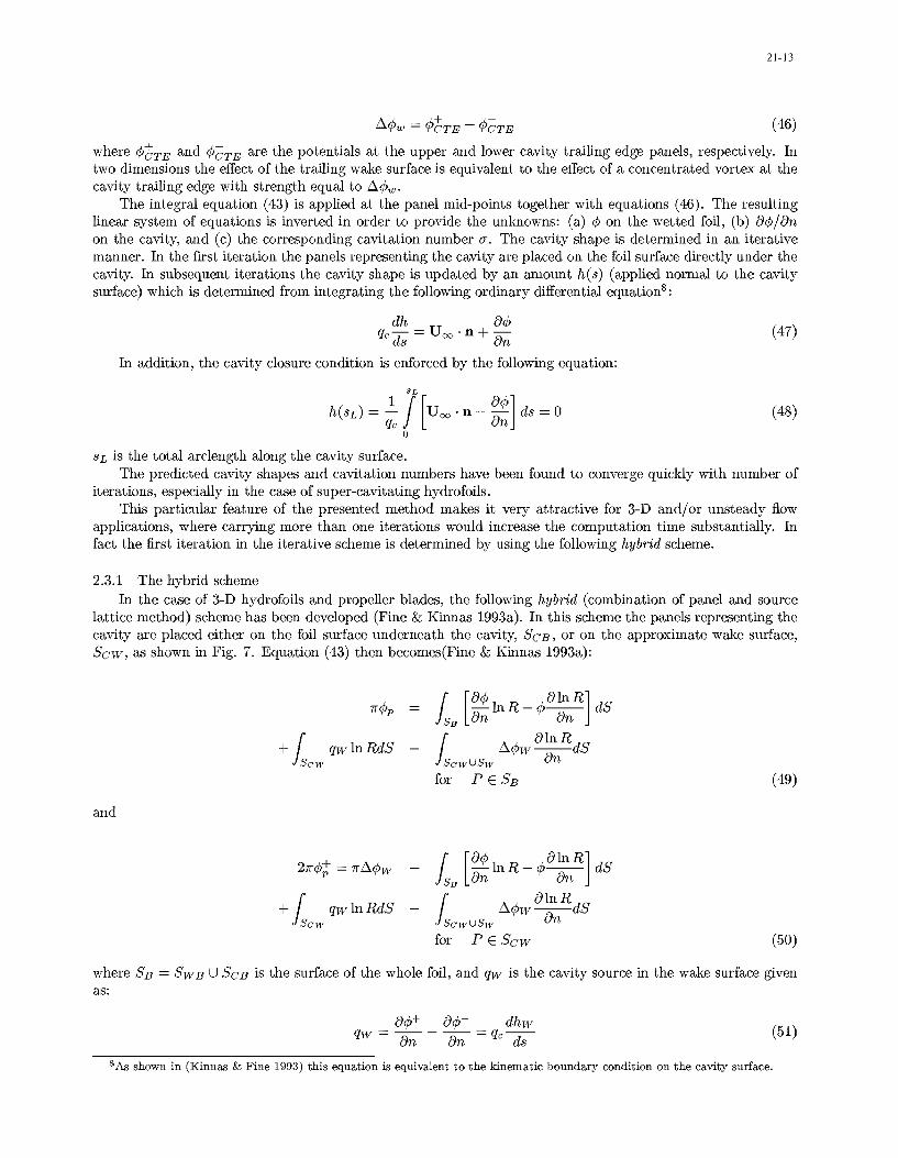
Figure 9: Predicted cavity trailing edge thickness and cavity shape for various cavity lengths at o = 1.097(corresponding to I = 0.4). From Kinnas and Fine, 1993.

where hw is the cavity height measured normal to Scw, as shown in Fig. 7. The cavity height h is measurednormal to the foil surface for the part of the cavity that overlaps the foil, as also shown in Fig. 7.

The major advantage of the hybrid scheme is that it can apply to all, wetted, partially, and super-cavitatingflows alike by utilizing the same panel discretization. In fact this scheme, as described in later sections, isapplied on super-cavitating 3-D hydrofoils and propellers. In addition, this scheme has been found to predictthe expected non-linear effect of foil thickness on the cavity shape in the case of partial cavitation (Kinnas &Fine 1993).

2.4 Cavity extent for given cavitation numberIn the previous sections the cavity length was assumed to be known. In the case of linear theory, equation

28 can be inverted with respect to I for given o. In the case of nonlinear theories the method can still be appliedfor the given or and various "trial" cavity lengths. In this case though, due to the fact that the cavitation numberis given (instead of being determined), the cavity closure condition, equation (48), or its equivalent hw(l) = 0in the case of the hybrid scheme, will not be satisfied.

h(1;o) =_ hw(l) 0 0 (52)

This is shown for a partially cavitating hydrofoil in Fig. 9 where the predicted J and the cavity shapes forfixed o and different values of cavity length are shown. An iterative scheme has been developed (Kinnas & Fine1993) for determining the cavity extent for given o by searching for the cavity length, 1, for which the cavitycloses (within a specified tolerance) at its trailing edge9 :

S= 0 (53)

A comparison of predictions from applying the linear, the fully non-linear, and the hybrid cavity models toa super-cavitating hydrofoil is shown in Figure 10. All theories, including the conventional linear theory, appear

9 An open cavity model can be readily implemented within this method by requiring the specified thickness at the cavity end.

21-15

020 -

) I

0.00 0.50 1.00 .50 2. C,,0

x/C

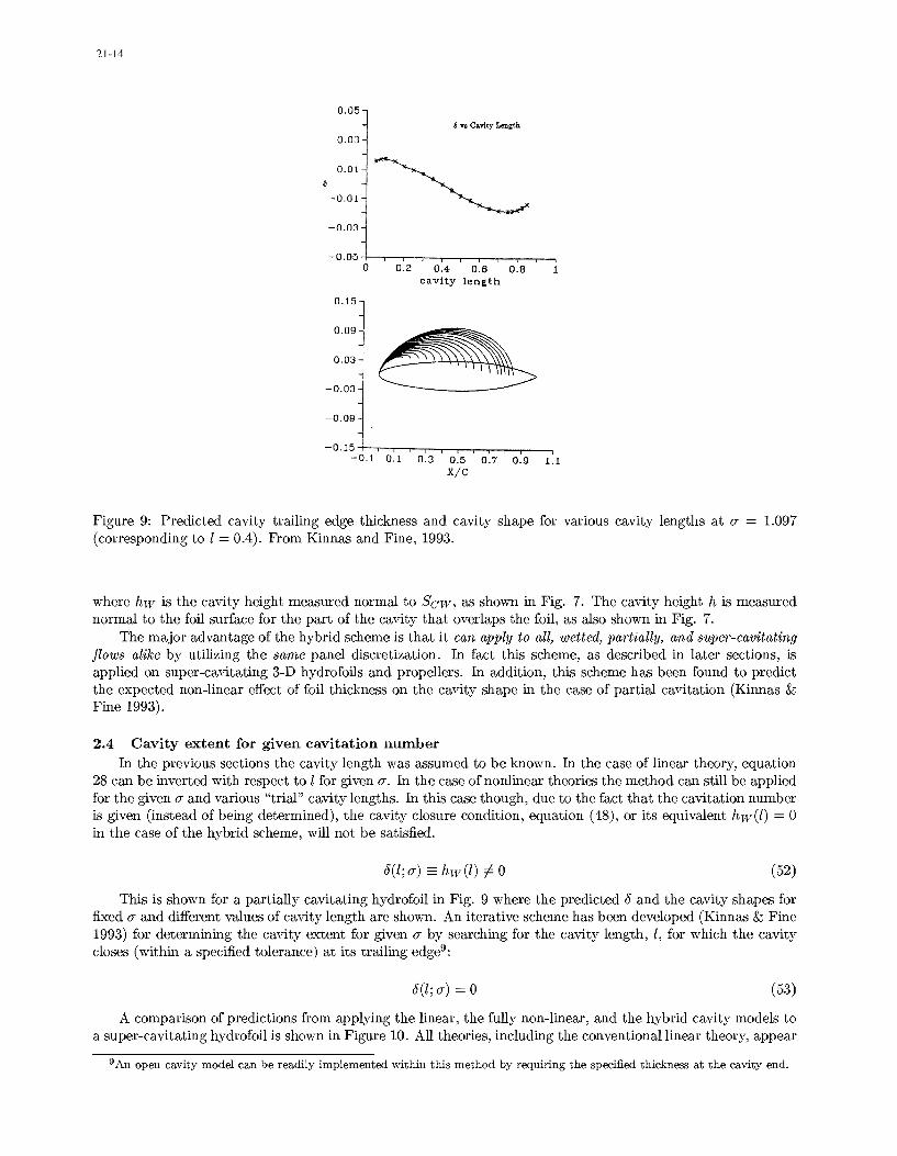
Figure 10: Comparison of predicted cavity shapes from linear (dashed), non-linear (solid) and hybrid (solidwith dots) theories for NACA16004 at a = 60. (dotted) linear; a/u = 0.44. From Fine and Kinnas (1993a).

to predict the cavity shape within satisfactory accuracy. Note that linear theory overpredicts the slope of thecavity at the leading edge.

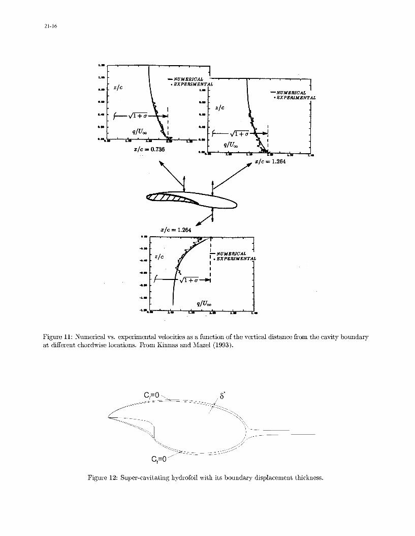
Finally, a comparison of predicted versus measured velocity profiles in the vicinity of a 2-D supercavityis shown in Figure 11. In the prediction the wall effects have been included by using a sufficient number ofmultiple images with respect to the horizontal tunnel walls (Kinnas & Mazel 1992).

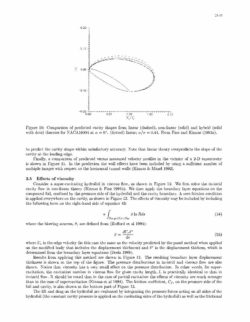
2.5 Effects of viscosityConsider a super-cavitating hydrofoil in viscous flow, as shown in Figure 12. We first solve the inviscid

cavity flow in non-linear theory (Kinnas & Fine 1991b). We then apply the boundary layer equations on thecompound foil, confined by the pressure side of the hydrofoil and the cavity boundary. A zero friction conditionis applied everywhere on the cavity, as shown in Figure 12. The effects of viscosity may be included by includingthe following term on the right-hand side of equation 43:

+ f USW In Rds (54)

where the blowing sources, &, are defined from (Hufford et al 1994):

- dUeJ*Sds (55)

where U, is the edge velocity (in this case the same as the velocity predicted by the panel method when appliedon the modified body that includes the displacement thickness) and P* is the displacement thickess, which isdetermined from the boundary layer equations (Drela 1989).

Results from applying this method are shown in Figure 13. The resulting boundary layer displacementthickness is shown at the top of the figure. The pressure distributions in inviscid and viscous flow are alsoshown. Notice that viscosity has a very small effect on the pressure distribution. In other words, for super-cavitation, the cavitation number in viscous flow for given cavity length, 1, is practically identical to that ininviscid flow. It should be noted that in the case of partial cavitation the effects of viscosity are much strongerthan in the case of supercavitation (Kinnas et al 1994). The friction coefficient, Cf, on the pressure side of thefoil and cavity, is also shown at the bottom part of Figure 13.

The lift and drag on the hydrofoil are evaluated by integrating the pressure forces acting on all sides of thehydrofoil (the constant cavity pressure is applied on the cavitating sides of the hydrofoil) as well as the frictional

21-16

Ll . .E .. . . .

- NUMERICAzic . EXPERIMENTAL N

C / -- NUMERICAL S• ,•''<' #cEXPERIMENTAL0.0 I.m

11 I L -EiE • I Ii-.

Cn Ca0.

e -a qS

xic =0.736 aft,-

xic =1.264

x/c- 1.264

L NUMERICALZ/C EXPERIMENTAL

-'LU

Figure 11: Numerical vs. experimental velocities as a function of the vertical distance from the cavity boundaryat different chordwise locations. From Kinnas and Mazel (1993).

Cf=O

Cf=O h

Figure 12: Super-cavitating hydrofoil with its boundary displacement thickness.

21-17

iic=O.04 Linear

fo/c=0.015 at p=0.85

a•=3.0'

I/c=3.0

Y/c

0 .1 -

0.0

-0.1

0 . . . x/c 34

0.2

0.0

-Cp

-0.2-

--- --- --- viscous-0.4 -0.4 -inviscid

0 . . . x/c 3 4

5.0

Cfx 1000

2.5

Cf=O

0.0 1 1 10 1 2 x/c 3 4

Figure 13: Super-cavitating hydrofoil in inviscid and viscous flow at Re = 2 x 107. Cavity shape and boundarylayer displacement thickness (top); pressure distributions (middle); and friction coefficient on the pressure sideof the foil and cavity (bottom). All predicted by the present method.

21-18

4.0T4c=O.04 Linear

I/c fo/c=0.015 at p=0.85

3.5- [x=3.0'

3.0

2.50.12 0.13 0.14 0.15 y 0.16

0.30-

CL

0.28-

0.26

02 Inviscid024 Re = 2.0 x 10 6

-........................ Re=2.0x 107

0 .2 2 , . . . . I . . . . I . . . . I . . . .I I . . .

0.12 0.13 0.14 0.15 G 0.16

0.03

Co _T TTi~iTi i;_illl-----------------ll

0.02

0.01

Inviscid- ------------ Re = 2.0 x 106-........................ Re = 2.0 x 107

0.00 1 . . . I . .. I . .. I ..0.12 0.13 0.14 0.15 G 0.16

Figure 14: Cavity length, lift and drag coefficient versus cavitation number for a super-cavitating hydrofoil ata = 30, in inviscid and viscous flow; predicted by the present method.

21-19

N G V/c2 CL CD

100 0.145 0.365 0.282 0.0219

160 0.146 0.364 0.287 0.0223

200 0.146 0.363 0.292 0.0231

Table 1: Convergence of viscous cavity solution (o, V/c 2 , CL and CD) with number of panels. Super-cavitatinghydrofoil; T/c = 0.045, fl/c = 0.015, p = 0.85, a = 3'.

FZSD

C

fo

p q

U. 0 P.o

Figure 15: The main parameters in the design of a super-cavitating hydrofoil.

forces acting on the wetted side of the hydrofoil. The convergence of the cavity solution and the predicted forceswith number of panels is given on Table 1.

Finally the predicted or, CL, and CD vs. I curves are shown in Figure 14, for a super-cavitating section ininviscid flow and for two Reynolds numbers'0 . The super-cavitating section is a combination of a NACA 4digitcamber form (with the maximum camber f, at x = p) and a linear thickness form. The effect of viscosity onlift coefficient is shown to be very small.

3 DESIGN OF SURER-CAVITATING SECTIONS3.1 Statement of the problem

We must determine the cavitating hydrofoil geometry and its operating condition (angle of attack, a), whichproduces the minimum drag, D, for specified design requirements.The parameters that define the geometry of a super-cavitating hydrofoil, also shown in Figure 15, are:

"* the chord, c

"* the maximum camber, fo, on the pressure side

"* the location of the maximum camber, fp

The design requirements taken into consideration in this paper are

1°Based on 1.

21-2C

"* Sectional lift, Lo(N/m)

"* Uniform forward velocity of the foil, U, (m/s)

"* Cavitation number, c0, defined as usual:

P7 -P;J (56)

where p is the fluid density, p,, is the ambient pressure, and pv is the vapor pressure.

"* Minimum section modulus of the foil, zmi

"* Acceptable cavity length, I

"* Acceptable cavity volume, V, or cavity height, h

The condition on the cavity length is necessary in order to avoid unstable cavities, usually being the longpartial or the short super-cavities. The cavity volume/height constraints ensures acceptable positive cavitythickness (volume) in order to avoid very thin cavities (also negative thickness cavities) which are either non-physical or may turn into harmful bubble cavitation.

3.2 The hydrodynamic coefficientsThe hydrofoil lift, L, and drag, D, acting on the hydrofoil, as shown in Figure 15, can be expressed in terms

of lift and drag coefficients, CL and CD, respectively:

12L = -IpU CCL (57)

2D = ½puiQCC (58)

The drag coefficient, CD, may be decomposed into two components.

CD = Cb + Cjj (59)

where Cb is the inviscid cavity drag coefficient, and Cb is the viscous drag coefficient.For known hydrofoil geometry, angle of attack, a, and cavity length, 1, any hydrodynamic or cavity quantity,

Q (CL, Cb, o7, V/c 2 ,....), may be expressed as follows:

Q = Q(a, nondimensional foil geometry, 1/c) (60)

Inviscid analysis methods are used to determine Q. The analytical formulas of (Hanaoka 1964) could havebeen used. These expressions though are based on linearized cavity theory, which has been found to overpredictthe cavity length and size substantially, especially in the case of partial cavitation. Instead, in this work thealready described numerical non-linear cavity analysis method is utilized (Kinnas & Fine 1991b, Kinnas & Fine1993). The shape of the cavity surface is determined in non-linear theory iteratively, with the use of a low-orderpotential based panel method. The (inviscid) forces are determined by integrating the pressures along the foilsurface.

The viscous drag is determined by assuming a uniform friction coefficient, Cf, over the wetted part of thefoil. Cf is expressed in terms of the Reynolds number (Re = Uc/lv, v : kinematic viscosity) via the ITTCformula (Comstock 1967):

0.075Cf = (logioRe - 2)2(61)

During the optimization process, the chord length (also the Reynolds number) is not known, thus the valueof Cf is updated at each optimization iteration.

Since only the lower surface of the foil determines the hydrodynamics of supercavitating flows, the thicknessis not included as a parameter. The upper surface can be placed anywhere arbitrarily inside the cavity. Thus,when computing the section modulus of a foil, the upper cavity surface is considered as the upper surface of the

21-21

"compound" foil. It is reasonable to assume that the cavity always starts at the leading edge of the foil, sincethe supercavitating sections have a sharp leading edge. Furthermore, we deal with situations where the cavitydetaches at the trailing edge of the foil on the pressure side. For the case of supercavitating sections, in additionto specifying the minimum section modulus of the compound section, the minimum allowable cavity height atthe 10% of the chord length from the leading edge is specified via an inequality constraint. This ensures positivecavity thickness, as well as sufficient local strength at the sharp leading edge of the foil.

The relevant coefficients are expressed as follows:

CL = CL(a,fo/c, fp/c,l/c)

Cb = Cb(a,fo/c, fp/c,l/c)o = u(a, folc, fplc, l1c)

V/c 2 = V/c2 (a,,fo/c, fp/c,l/c)z/c 3 = z/c 3 (a, fo/c, fp/c,l/c)

h1 o/c = h1 o/c(a, fo/c, fp/c, i/c)

where h1o is the cavity height at the 10% of the chord length from the leading edge of the foil. Note that thesection modulus is a function of all the geometry variables including the cavity length, whereas it is independentof the cavity length in the case of partial cavitation.

The coefficients are computed, as in the case of partial cavitation, for a number of foil geometries by usingthe analysis method of (Fine & Kinnas 1993a). The coefficients are again expressed by using second degreepolynomials in terms of all the geometric parameters. For example,

C C C ±CA (fo)2

±CL 9 & = CL1a + ±C L1 1 a-±+CL4 -

C cCe c

--- + CL-,, + CL1 5 (62)C C C C

where,

-' 1 (63)C 1- (C/1)2 + I -- (C/1)2

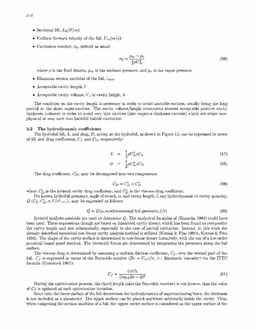
The variable transformation from i/c to I'/c is done knowing that CL and CD are linear in I'/c for thesuper-cavitating flat plate in linear theory, as described by (Geurst 1960). This transformation has been foundto improve the accuracy of the interpolation substantially. The effect of the number of The accuracy of theinterpolation for CD may be seen in Figures 16.

3.3 The optimization problemConsider the following general nonlinear optimization problem:

minimize f (x)

subjectto gi(x) <0 i=1,2,..,mhi(x)=0 i=1,2,...,i (64)

where f(x) is the objective function defined on RZ. x is the solution vector of n components. g1 (x) <0,---, gm.(x) < 0 are inequality constraints defined on R'Z and hi(x) = 0, h, h,(x) = 0 are equality constraintsalso defined on R'.

The solution vector is defined as (n = 5):

x = [a, c, fo, fp, 1]T (65)

21-22

The constraints are (m = 3,1 = 2)

hi(x) = L(x)-Lo=0 (66)

h2 (x) = O(x)-O0=0 (67)

g+ (x) = - I + <0 (68)C ri

g2 (x) - z(x) Zin < 0 (69)

g3 (x) - hi o(x) + (± o _< 0 (70)C \C !rain

3.4 The numerical optimization methodThe method of multipliers is applied in which, first each of the inequality contraints, gi (x) • 0, is converted

into an equality constraint with the introduction of the new variable, si:

gj(x) + s? = 0 (71)

Then the augmented Langrangian penelty function is formed (Mishima & Kinnas 1996):

F ( x l , . . ., s1 , . . . , /k l , . .. , ý 1 , ---, ý c l ,. . . , 5ý 1 ,. . .) =

D(x) + ±Aihi(x)+ + A[gi(x) + s?]

±Ecih?(x) + +aigi(X) + 8?]2 (72)

where A• and A, are the Langrange multipliers, and ci and ýi are penalty parameters. The parameters of theproblem, the additional parameters (si), the Langrange multipliers, and the penalty parameters are determinedby minimizing function F. A technique to minimize F is described in great detail in (Mishima & Kinnas 1996).

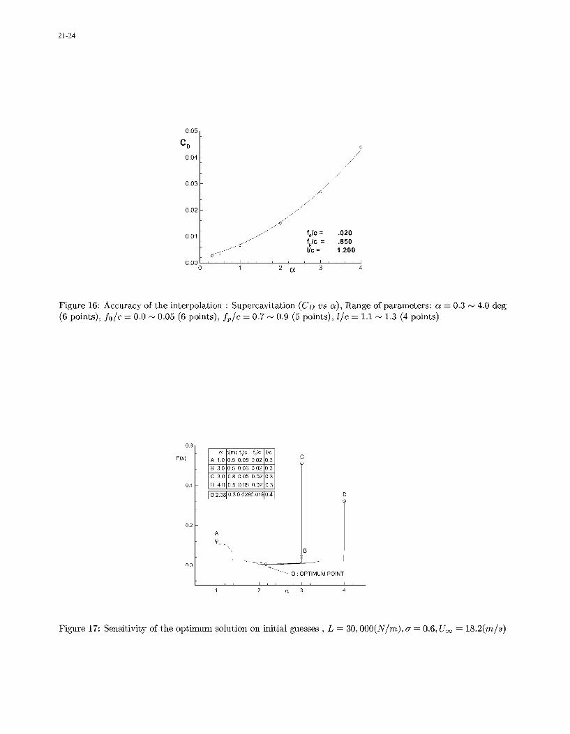
3.5 Effect of the initial guess on the optimum solutionIn general, a nonlinear optimization problem is initial guess dependent. In other words, if there exist more

than one local minimum to the objective function, any one of these minima may be obtained depending on theinitial condition. Due to the special structure of the problem, no multiple solutions were found for the range ofcavitation numbers that we studied. This uniqueness is attributed partly to the fact that the involved functionsare quadratic, i.e. not wavy, and partly to the fact that the range of the solutions is known, so that a reasonableinitial guess can be selected. Figure 17 shows that several different initial guesses lead to the same solution.

3.6 ResultsA NACA 4 digit camber form and the Johnson five-term camber form are used. The NACA 4digit camber

form (Abbott & Von Doenhoff 1959) has two parameters, which are the maximum camber fo/c and the locationof the maximum camber fp/c, as shown in Figure 15. The values for the constraints are:

(l) =1.15 (- =) 0.01 Zrn)= 7 x 10-5 (73)c rain C rain ( c3]

The method is applied for fixed lift (L0 = 30, OOON/m) and for a range of cavitation numbers between0.15 and 0.7 (corresponding to approximate speeds of 70 and 30 knots, respectively") for partial and super-cavitating conditions. The resulting L/D for both cases are shown in Figure 18. As expected, for "low" o asupercavitating section has larger L/D than a partially cavitating section, and the reverse holds for larger or.Optimum partially and supercavitating sections are also shown in Figure 18.

Finally, we show in Figure 19, contour plots of LID for optimum sections, designed by the present method,over a range of combinations of required lift and cavitation number. This graph is intended to help the designerdecide as to what is the best solution (partially or supercavitating section), depending on the requirements.

"The cavitation number is inversely proportional to the square of the speed of the hydrofoil, for fixed ambient pressure andtemperature conditions.

21-23

3.7 Comparison of the present to existing design methodsThe designed sections, under given requirements, are compared to those designed from other methods.

These methods are based on either the Tulin two-term or the Johnson five-term sections, given next:

=- + 3 c -- 4 c (Tulin two-term) (74)

(Johnson five - term) (75)

where A1 is a parameter that relates the geometry to the lift coefficient.As the number of terms included in the series increases, the loading moves towards the trailing edge. A

useful formula for the finite cavitation number correction is given by (Ohba 1963/1964) as follows.

CL[= 10 L 0"854 2 +12600 (76)

where CL is the required lift coefficient and CL,=o0 is the lift coefficient for zero cavitation number.In Figure 20, the lift to drag ratio, L/D, is shown for the NACA 4dgt sections designed by the present

method, Tulin's two-term sections, and Johnson's five-term sections, for various cavitation numbers. In thesame figure we also show the L/D for the optimum Johnson section as designed by the present method. Thecorresponding lift coefficients are shown in Figure 21. For the design of Tulin sections and Johnson sections,the cavitation number and the lift coefficient are both specified, whereas in the present method, the cavitationnumber and the lift are given and the lift coefficient is determined as part of the solution. A representative

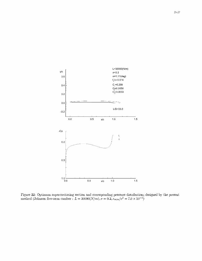
section and its corresponding pressure distribution is shown in Figure 22.

3.8 Application to 3-D elliptic planform hydrofoilsAs shown in (Kinnas et al 1995), a super-cavitating hydrofoil with elliptic planform and similar sections

along its span (that are only scaled by the chord), can be designed by designing an equivalent 2-D section. If cand s, are the maximum chord and span of the elliptic wing, the equivalent 2-D lift is given from:

4L2D = L3D (77)

If D2D is the corresponding minimum value of the drag then D3D will be given as:

L 3D 78 0 D (78)D3D= 1/2pU ± +--D-

(T+)The above equation can be re-written as:

D3D L3D D2D

L3D 1/2pU,2s, L2D

Equation (79) implies that (L/D)3D will always be smaller than (L/D)2D, i.e. the 3-D hydrofoil will alwaysbe less efficient than the 2-D hydrofoil.

The actual angle of attack a3D will be related to that determined from the 2-D equivalent optimizationproblem as:

a3D = a2D + 1/2pUL3sD (80)

21-24

0.05

CD

0.04 -

0.03 -

0.02

0.01 f/c= .020fp/c = .850I/c= 1.200

0 .0 0 . . .. .0 1 2 a 3 4

Figure 16: Accuracy of the interpolation : Supercavitation (CD vs a), Range of parameters: a = 0.3 - 4.0 deg(6 points), fo/c = 0.0 - 0.05 (6 points), fp/c = 0.7 - 0.9 (5 points), i/c = 1.1 - 1.3 (4 points)

0.6

zx X (m t0/c fjc I/cF(x) A 1.0 0.5 0.05 0.02 0.3

B 3.0 0.5 0.05 0.02 0.3

C 3.0 0.8 0.05 0.02 0.3

0.4 D 4.0 0.5 0.05 0.02 0.3

1012.08 0.310.0210.0110.4 D

0.2

A

B

0.000 : OPTIMUM POINT

2 (X 3 4

Figure 17: Sensitivity of the optimum solution on initial guesses, L = 30, O00(N/m), r = 0.6, U, = 18.2(m/s)

2 1-25

100- Partial cavitationBL/D

50-

0.2 0.4 (7 0.6

Solution B a 2.1deg

y/000.02

0.0

c 0.20my/b0 .4 f,/c 0.011

0.2 fp/c 0.82

0.01

0.0 0.5 x/c 1.'0 1.5

Figure 18: L/D for partially or super-cavitating foils designed by the present method; LO 30, OOON/m.

_____ partially cavitating

--- -supJercavitating

L (Min) 0 0

40000

30000

20000 -

20000

0.2 0.4 G 0.6

Figure 19: Contour plots of LID for partially or super-cavitating foils designed by the present method.

21-26

40 Johnson 5term camber(Present design method)

L/D /

30------

Johnson 5term camber NACA 4digit camber(Present design method)

20 A A

Tulin 2term camber

0.2 G 0.3

Figure 20: Comparison of L/D between designed sections and existing sections (L = 30000(N/m), zmi!c =

7.0 x 10-5 (supercavitating)

0.8NACA 4digit camber(Present design method)

CL

0.6

Johnson 5 term camber

0.4-

0.2 Johnson 5 term camber(Present design method)

0.2 ,

Tulin 2 term camber

0.00.2 G 0.3

Figure 21: Comparison of CL between designed sections and existing sections (L = 30000(N/m), zmin!c 3 =

7.0 x 10-5 (supercavitating)

21-27

L=30000(N/m)y/c (T=0.2

0.6 (x=1.1 l(deg)fo/c=0.014

0.4 CL=0.299C,=0.0058C.=0.00330.2

0.0

L/D=33.0-0.2

0.0 0.5 x/c 1.0 1.5

-Cp

0.0

-0.5

-1.00.0 0.5 x/c 1.0 1.5

Figure 22: Optimum supercavitating section and corresponding pressure distribution; designed by the presentmethod (Johnson five-term camber : L = 30000(N/m), a = 0.2, zmin/c 3 = 7.0 x 10-5)