defining and running counterfactual scenarios using isim-mams · to exogenous policy and external...

-1-

Defining and Running Counterfactual Scenarios Using

ISIM-MAMS*

This material was prepared by Martín Cicowiez (CEDLAS-UNLP) and Marco V. Sánchez (UN-DESA) for the

First Intensive Training Workshop of the Project “Strengthening Macro-Micro Modeling Capacities to

Assess Development Support Measures and Strategies”, Entebbe, March 7-9, 2012, which has been

organized by UNDP Uganda, the Ministry of Finance Planning and Economic Development (MOFPED)

and UN-DESA.

1. Exogenous Policy and External Shocks Simulations

In this session, we will show, step by step, how to define and run four counterfactual scenarios related

to exogenous policy and external shocks using ISIM-MAMS with the Uganda 2009/10 dataset (updated

as of March 2012). In order to implement the following examples, the reader should have successfully

installed ISIM-MAMS.

Example 1: Increase in the world export price of food products during 2011-

2015

In this first example, we will start by creating the ISIM-MAMS application file that will be used

throughout the remaining of the workshop (see steps 1-3). Then, we will define and run a scenario that

simulates a 50% increase in the world export price of food during 2011/12-2015/16.

1. Open Excel.

2. Click on the ISIM-MAMS tab; it automatically opens a ribbon with MAMS-specific buttons.

3. Click on Newin the Application ribbon group (Figure 1.1). Then,

1. Introduce the name Test for the new MAMS application.

2. Select the Uganda0910 dataset.

3. Select the MDG version of MAMS (Figure 1.2).

*ISIM-MAMS (An Interface for MAMS (MAquette for MDG Simulations)) was developed for The World Bank Development

Economics Prospect Group (DECPG); Hans Lofgren from the World Bank is key author of the MAMS program code.

-2-

Figure 1.1: Create a New ISIM-MAMS Application 1

Figure 1.2: Create a New ISIM-MAMS Application 2

4. Run the pre-programmed reference scenario by clicking on Run Setup in the Setup ribbon group.

MAMS will be run and a window will show the progress in running MAMS (Figure 1.3). Tip: you may

like to check what closure and rules are being used in order to understand the results generated for

this pre-programmed reference scenario (it is important to do so, as this is the benchmark taken for

all other simulations!).

Figure 1.3: Running Model Setup

5. Open the Scenario Manager by clicking on Scenario Manager in the Simulations ribbon group.

Then, click on New simulation to create a new simulation. In the window that shows up (Figure 1.4),

-3-

1. Introduce “pwefood” (i.e., the name we want to give to this example simulation) in the Name

field.

2. Introduce a short description in the Description field, which is good to associate the simulation

with the change eventually imposed.

3. Keep the Multi-pass default in the Mode field. Once finished, click OK. The newly created

simulation will be added to the Scenario Manager (Figure 1.5).

Figure 1.4: Defining the New Simulation

Figure 1.5: Scenario Manager

6. Go to the pwesim section in the external-shocks sheet. Note that the Navigation Tree can be used

to move across the Excel file (Figure 1.6); to access the Navigation Tree, click on the corresponding

icon on the View ribbon group. To define the counterfactual scenario,

1. In column sim (i.e., simulation), use the drop-down menu to select pwefood (i.e., the name that

had been given to the simulation).

-4-

2. In column c (i.e., commodity), use the drop-down menu to select one of the agricultural

commodities – see the dictionary sheet in order to identify the agricultural commodities in the

Uganda 2009/10 SAM.

3. Click on Add row to add a new row to the pwesim shock parameter and then select one of the

remainder agricultural commodities; repeat this step until all 18 agricultural commodities that

are part of the Uganda dataset are included as part of the pwefood simulation (c-maize, c-rice, c-

wheat, c-cassava, c-potato, c-cotton, c-tobacco, c-beans, c-flowers, c-coffee, c-tea, c-matoke, c-

othagr, c-livestock, c-fish, c-othfood, c-coffeeproc, c-teaproc).1

4. In columns 2009-2010, introduce number 1 (i.e., keep the base year value) for all the selected

agricultural commodities (Figure 1.6). Notice that the default simulation period for the

Uganda0910 dataset is 2009/10-2015/16, with 2009/10 being the base year.

5. In columns 2011-2015, introduce 1.25 (i.e., the equivalent to 25% in the ISIM-MAMS setting) for

all the selected agricultural commodities.

Figure 1.6: Navigation Tree and Defining Shocks to the World Price of Exports

7. Run the selected simulations by clicking on Run in the Simulations ribbon group. Again, a window

will show the progress in running MAMS.

8. Once finished, new sheets with reports will be added to the Excel file. The user can access the

results through macro and meso reports, the dashboard, and a pivot table (Figure 1.7). Note that

the repmacro-contents and repmeso-contents sheets can be used to navigate across the report

tables.

9. Analyze the macro and meso results. Specifically, review the following results: macro aggregates,

real exchange rate, government budget, sectoral structure of production and trade, and MDG

indicators. Once finished, you can save the ISIM-MAMS application Excel file by following the Excel

1 In reality, the simulation of a world price should affect both the export price and the import price of the commodity if

this commodity is both exported and imported. Up to this point, we want to simulate a shock in the world export price

only. In the two subsequent examples, we respectively shock the world import price only (example 2) and both world

export and import prices (example 3). Simulating separately the shocks in world export and import prices for a

commodity that is both exported and imported allows a better understanding of the results of a shock when both prices

are changed simultaneously (where there is also interaction effects from changing both prices).

-5-

usual procedure (i.e., go to File | Save). Note that an ISIM-MAMS application Excel file is always

associated with a country-specific dataset.

Figure 1.7: Report Example

Example 2: Increase in the world import price of agricultural products

In this example, we start from the last step of example 1. Thus, there is no need to create a new ISIM-

MAMS application Excel file and/or run the pre-programmed reference scenario.


Then, click on New simulation to create a new simulation. In the window that shows up,

1. Introduce “pwmfood” to stand for the name of this new simulation in the Name field.

2. Introduce a short description in the Description field.

3. Keep the Multi-pass default in the Mode field. Once finished, click OK. The newly created

simulation will be added to the Scenario Manager.

2. Go to the pwmsim section in the external-shocks sheet. To define the counterfactual scenario,

follow steps 6.1-6.5 of the previous example but using the pwmsim shock parameter and the

pwmfood simulation. Note that you can copy the list of food commodities from the definition of the

pwesim shock parameter used in the previous example.

3. Run the selected simulations by clicking on Run in the Simulations ribbon group. Again, a window

will show the progress in running MAMS.

4. Once finished, the report sheet will be updated, including results for simulations pwefood and

pwmfood, and the file can be saved.

5. Analyze the macro and meso results; specifically, review the following results: macro aggregates,

real exchange rate, government budget, sectoral structure of production and trade, and MDG

indicators.

-6-

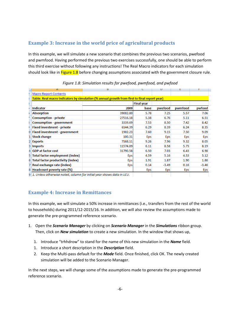
Example 3: Increase in the world price of agricultural products

In this example, we will simulate a new scenario that combines the previous two scenarios, pwefood

and pwmfood. Having performed the previous two exercises successfully, one should be able to perform

this third exercise without following any instructions! The Real Macro indicators for each simulation

should look like in Figure 1.8 before changing assumptions associated with the government closure rule.

Figure 1.8: Simulation results for pwefood, pwmfood, and pwfood

Example 4: Increase in Remittances

In this example, we will simulate a 50% increase in remittances (i.e., transfers from the rest of the world

to households) during 2011/12-2015/16. In addition, we will also review the assumptions made to

generate the pre-programmed reference scenario.


Then, click on New simulation to create a new simulation. In the window that shows up,

1. Introduce “trhhdrow” to stand for the name of this new simulation in the Name field.


2. Keep the Multi-pass default for the Mode field. Once finished, click OK. The newly created


In the next steps, we will change some of the assumptions made to generate the pre-programmed

reference scenario.

-7-

2. Go to the siclossim section in the closure-and-rules sheet to change the saving-investment. Then,

1. In column sim, select trhhdrow.

2. In column 2009, select 1 (can you explain the meaning of option 1?); note that option 1 will be

applied to the whole simulation period.

3. Go to the govclossim section in the closure-and-rules sheet to change the government closure.

Then,


4. In column 2009, select 5 (can you explain the meaning of option 5?).

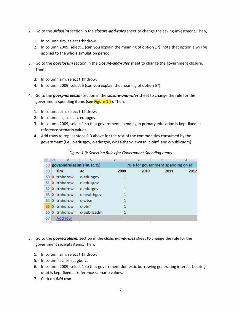
4. Go to the govspndrulesim section in the closure-and-rules sheet to change the rule for the

government spending items (see Figure 1.9). Then,


2. In column ac, select c-edupgov.

3. In column 2009, select 1 so that government spending in primary education is kept fixed at

reference scenario values.

4. Add rows to repeat steps 2-3 above for the rest of the commodities consumed by the

government (i.e., c-edusgov, c-edutgov, c-healthgov, c-wtsn, c-oinf, and c-publicadm).

Figure 1.9: Selecting Rules for Government Spending Items

5. Go to the govrecrulesim section in the closure-and-rules sheet to change the rule for the

government receipts items. Then,


5. In column ac, select gborz.

6. In column 2009, select 1 so that government domestic borrowing generating interest-bearing

debt is kept fixed at reference scenario values.

7. Click on Add row.

-8-

2. On the new row, in column sim, select trhhdrow.

8. On the new row, in column ac, select gbormsz.

9. On the new row, in column 2009, select 1 so that government domestic borrowing via the

monetary system (i.e., non-generating interest-bearing debt) is kept fixed at reference scenario

values.



12. On the new row, in column ac, select fborgov.

13. On the new row, in column 2009, select 1.



16. On the new row, in column ac, select trgovrow.

17. On the new row, in column 2009, select 1.

6. Go to the ngovpayrulesim section in the closure-and-rules sheet to change the rules for the

different non-government payments (see Figure 1.10). Then,


2. In column ac, select trngovrow (aggregate transfers to non-government institutions from rest of

world).

3. In column 2009, select 1 so that the trnsfrpcsim shock parameter can be used to define the

counterfactual increase in remittances.

4. Add rows to repeat steps 2-3 above for the following non-government payments: trfacrow

(aggregate transfers to factors from the rest of the world), fborngov (aggregate non-government

borrowing from the rest of the world), and fdiz (foreign direct investment). Doing this, this set of

non-government payments will be kept fixed at reference scenario values.

Figure 1.10: Selecting Rules for Non-Government Payments

7. Go to the trnsfrpcsim section in the trnsfr-shocks sheet (Figure 1.11). To define the counterfactual

scenario,


-9-

2. In column h (i.e., households), select hhd – note that the current version of the Uganda 2009/10

SAM identifies only one household.

3. In columns 2009-2010, introduce 1 (i.e., keep the base year value).

4. In columns 2011-2015, introduce 1.5 so that remittances per capita are increased by 50% relative

to the reference scenario values.

Figure 1.11: Defining Shocks to Per-Capita Transfers to Households

8. Run the new simulation by clicking on Run in the Simulations ribbon group.

9. As before, the report sheets will be overwritten with the new set of results. As an example, some

results are shown in Table 1.1.

Table 1.1: Simulation Results for trhhdrow; real macro indicators by simulation (% annual growth from

first to final report year)

Final year

Indicator 2009 base trhhdrow

Absorption 39,003 5.78 6.12

Consumption - private 27,516 5.38 5.77

Consumption - government 3,340 7.53 7.53

Fixed investment - private 6,144 6.29 6.66

Fixed investment - government 1,902 7.60 7.62

Stock change 100 0.00 0.00

Exports 7,168 9.26 8.39

Imports 11,575 6.11 6.34

GDP at factor cost 31,791 6.50 6.57

Total factor employment (index) 4.59 4.64

Total factor productivity (index) 1.91 1.93

Real exchange rate (index) 0.14 0.07

-10-

Table 1.2: Simulation Results for trhhdrow; government receipts and spending in first report year and by

simulation in final report year (% of nominal GDP)

Final year

Indicator 2009 base trhhdrow

Receipts Direct taxes 3.98 3.98 3.98

Import tariffs 5.86 5.86 5.86

Export taxes Eps Eps Eps

Other indirect taxes 2.25 2.25 2.25

Private transfers 0.35 0.35 0.35

Foreign transfers 2.63 2.63 2.61

Factor income 0.04 0.02 0.02

Domestic borrowing 2.32 2.32 2.30

Foreign borrowing 2.47 3.67 3.63

Total 19.90 21.09 21.01

Spending Consumption 9.65 10.26 10.21

Fixed investment 5.50 5.92 5.89

Stock change Eps Eps Eps

Private transfers 3.63 3.63 3.63

Foreign transfers 0.01 0.01 0.01

Domestic interest payments 0.94 0.96 0.95

Foreign interest payments 0.17 0.32 0.31

Domestic capital transfers Eps Eps Eps

Total 19.90 21.09 21.01

2. Support measures simulations

In this session, we will show, step by step, how to define and runcounterfactual scenarios related to

support measuresusing the Uganda 2009/10 dataset. Thus, the following assumes that the reader has

successfully created an ISIM-MAMS application Excel file using the Uganda0910 dataset; certainly, the

Excel file from the previous set of examples can be used – and just make sure it was saved.

Example 1: Increase in foreign transfers (aid) channeled to the financing of human

development spending

In this example, we will define and run a scenario that simulates an increase in foreign aid during

2011/12 – 2015/16 that is channeled to the financing of human development spending (i.e., education,

health and water and sanitation).

1. Create a new simulation using the Scenario Manager in the Simulations ribbon group. Then, click on

New simulation. In the window that shows up,

1. Introduce “aid-hd” (as before, the name of the newly-created simulation) in the Name field.

-11-




2. Go to the siclossim section in the closure-and-rules sheet to change the saving-investment closure.

Then,

1. In column sim, select aid-hd.

2. In column 2009, select 1.

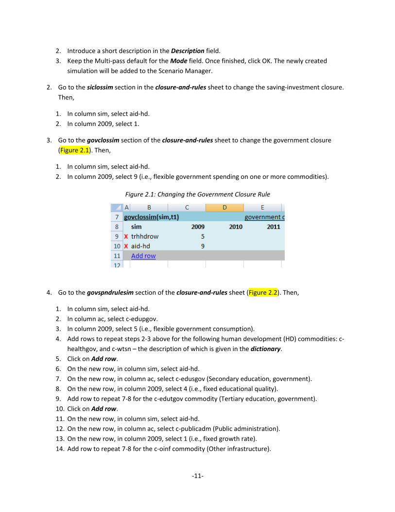
3. Go to the govclossim section of the closure-and-rules sheet to change the government closure

(Figure 2.1). Then,


2. In column 2009, select 9 (i.e., flexible government spending on one or more commodities).

Figure 2.1: Changing the Government Closure Rule

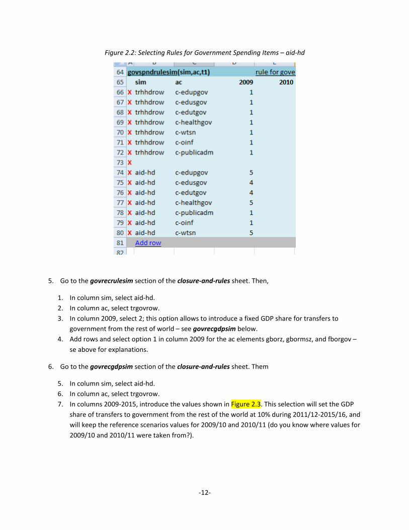
4. Go to the govspndrulesim section of the closure-and-rules sheet (Figure 2.2). Then,


2. In column ac, select c-edupgov.

3. In column 2009, select 5 (i.e., flexible government consumption).

4. Add rows to repeat steps 2-3 above for the following human development (HD) commodities: c-

healthgov, and c-wtsn – the description of which is given in the dictionary.


6. On the new row, in column sim, select aid-hd.

7. On the new row, in column ac, select c-edusgov (Secondary education, government).

8. On the new row, in column 2009, select 4 (i.e., fixed educational quality).

9. Add row to repeat 7-8 for the c-edutgov commodity (Tertiary education, government).


11. On the new row, in column sim, select aid-hd.

12. On the new row, in column ac, select c-publicadm (Public administration).

13. On the new row, in column 2009, select 1 (i.e., fixed growth rate).

14. Add row to repeat 7-8 for the c-oinf commodity (Other infrastructure).

-12-

Figure 2.2: Selecting Rules for Government Spending Items – aid-hd

5. Go to the govrecrulesim section of the closure-and-rules sheet. Then,


2. In column ac, select trgovrow.

3. In column 2009, select 2; this option allows to introduce a fixed GDP share for transfers to

government from the rest of world – see govrecgdpsim below.

4. Add rows and select option 1 in column 2009 for the ac elements gborz, gbormsz, and fborgov –

se above for explanations.

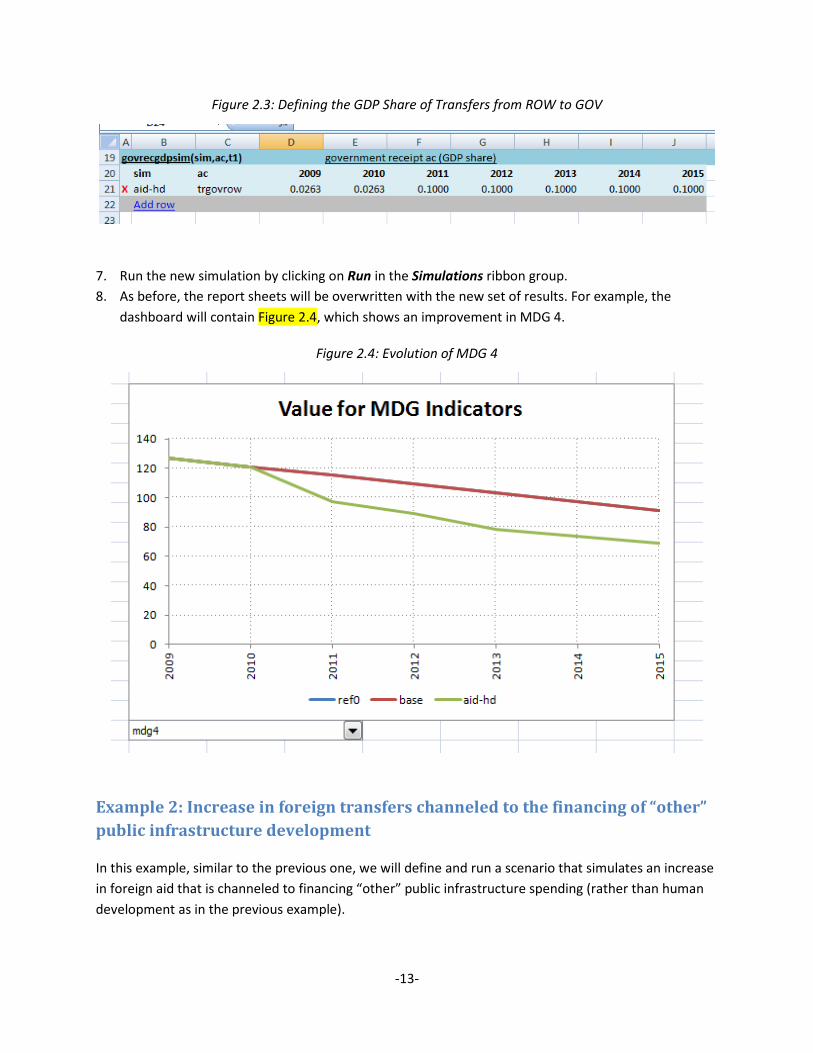
6. Go to the govrecgdpsim section of the closure-and-rules sheet. Them


6. In column ac, select trgovrow.

7. In columns 2009-2015, introduce the values shown in Figure 2.3. This selection will set the GDP

share of transfers to government from the rest of the world at 10% during 2011/12-2015/16, and

will keep the reference scenarios values for 2009/10 and 2010/11 (do you know where values for

2009/10 and 2010/11 were taken from?).

-13-

Figure 2.3: Defining the GDP Share of Transfers from ROW to GOV

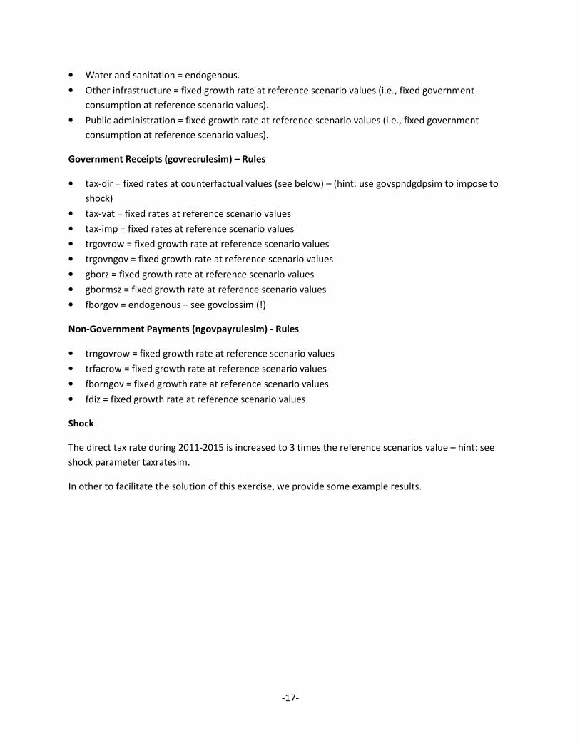
7. Run the new simulation by clicking on Run in the Simulations ribbon group.

8. As before, the report sheets will be overwritten with the new set of results. For example, the

dashboard will contain Figure 2.4, which shows an improvement in MDG 4.

Figure 2.4: Evolution of MDG 4

Example 2: Increase in foreign transfers channeled to the financing of “other”

public infrastructure development

In this example, similar to the previous one, we will define and run a scenario that simulates an increase

in foreign aid that is channeled to financing “other” public infrastructure spending (rather than human

development as in the previous example).

-14-

1. Create a new simulation using the Scenario Manager in the Simulations ribbon group. Then, click on

New simulation. In the window that shows up,

1. Introduce “aid-infra” in the Name field.




The remaining steps are similar to those of the previous example, but in this case the government

consumption of c-oinf (i.e., Other public infrastructure) should be left flexible. What options should you

select in govspndrulesim for the other commodities consumed by the government?

Note that a comparison of results between the present scenario and the previous one is not

straightforward; can you explain why? Hint: compare the evolution of GDP and foreign transfers in both

scenarios.

3. Additional Exercises

Exercise 1

What assumption has been made for the evolution of tax receipts in the previous scenarios? Is this a

reasonable assumption? Now, create additional simulations in order to run the world price scenarios

using the following alternative closure and rules assumptions:

Closure

• Government Closure (govclossim) = direct tax rate is the clearing variable for the government

budget.

• Savings-Investment Closure (siclossim) = household investment is the clearing variable (i.e.,

endogenous real growth, GDP and absorption shares).

Government Spending (govspndrulesim) - Rules

• Primary education = fixed quality at reference scenario values.

• Secondary education = fixed quality at reference scenario values.

• Tertiary education = fixed quality at reference scenario values.

• Health = fixed growth rate at reference scenario values (i.e., fixed government consumption at

reference scenario values).

• Water and sanitation = fixed growth rate at reference scenario values (i.e., fixed government

consumption at reference scenario values).

• Other infrastructure = fixed growth rate at reference scenario values (i.e., fixed government


-15-

• Public administration = fixed growth rate at reference scenario values (i.e., fixed government


Government Receipts (govrecrulesim) – Rules

• tax-dir = endogenous – see govclossim (!)

• tax-vat = fixed rates at reference scenario values

• tax-imp = fixed rates at reference scenario values

• trgovrow = fixed growth rate at reference scenario values

• trgovngov = fixed growth rate at reference scenario values

• gborz = fixed growth rate at reference scenario values

• gbormsz = fixed growth rate at reference scenario values

• fborgov = fixed growth rate at reference scenario values

Non-Government Payments (ngovpayrulesim) - Rules

• trngovrow = fixed growth rate at reference scenario values

• trfacrow = fixed growth rate at reference scenario values

• fborngov = fixed growth rate at reference scenario values

• fdiz = fixed growth rate at reference scenario values

In other to facilitate the solution of this exercise, we provide some example results.

Table 3.1: Simulation Results for trhhdrow; real macro indicators by simulation (% annual growth from

first to final report year)

Final year

Indicator 2009 base

pwefood-

ex

pwmfood-

ex

pwfood-

ex

Absorption 39,003 5.78 6.64 5.60 6.47

Consumption - private 27,516 5.38 6.48 5.12 6.24

Consumption - government 3,340 7.53 7.17 7.60 7.24

Fixed investment - private 6,144 6.29 7.12 6.20 7.03

Fixed investment - government 1,902 7.60 7.43 7.60 7.43

Stock change 100 Eps Eps Eps Eps

Exports 7,168 9.26 9.24 9.22 9.24

Imports 11,575 6.11 8.23 5.73 7.83

GDP at factor cost 31,791 6.50 6.76 6.43 6.71

Total factor employment (index) Eps 4.59 4.85 4.55 4.82

Total factor productivity (index) Eps 1.91 1.91 1.89 1.89

Real exchange rate (index) Eps 0.14 -3.40 0.15 -3.38

-16-

Table 3.2: Simulation Results for trhhdrow; government receipts and spending in first report year and by

simulation in final report year (% of nominal GDP)

Final year

Indicator 2009 base

pwefood-

ex

pwmfood-

ex

pwfood-

ex

Receipts Direct taxes 3.98 3.98 3.99 3.98 3.99

Import tariffs 5.86 5.86 4.95 5.89 4.97

Export taxes Eps Eps Eps Eps Eps

Other indirect taxes 2.25 2.25 2.24 2.26 2.25

Private transfers 0.35 0.35 0.35 0.35 0.35

Foreign transfers 2.63 2.63 2.05 2.65 2.06

Factor income 0.04 0.02 0.02 0.02 0.02

Domestic borrowing 2.32 2.32 2.17 2.36 2.21

Foreign borrowing 2.47 3.67 3.75 3.75 3.80

Total 19.90 21.09 19.51 21.27 19.65

Spending Consumption 9.65 10.26 9.41 10.40 9.52

Fixed investment 5.50 5.92 5.28 5.94 5.29

Stock change Eps Eps Eps Eps Eps

Private transfers 3.63 3.63 3.63 3.63 3.63

Foreign transfers 0.01 0.01 0.01 0.01 0.01

Domestic interest payments 0.94 0.96 0.90 0.98 0.91

Foreign interest payments 0.17 0.32 0.29 0.32 0.29

Domestic capital transfers Eps Eps Eps Eps Eps

Total 19.90 21.09 19.51 21.27 19.65

Exercise 2

In this exercise, you will create a new scenario in order to simulate the creation of fiscal space through

an increase in direct tax collection. Then, the additional fiscal space will be to finance government

spending in (a) human development, or (b) infrastructure. The following assumptions should be applied:

Exercise 2.a description

Government Closure = government spending is the clearing variable for the government budget.

Savings-Invesment Closure = same as exercise 1

Government Spending (govspndrulesim) - Rules

• Primary education = endogenous.

• Secondary education = fixed quality at reference scenario values.

• Tertiary education = fixed quality at reference scenario values.

• Health = endogenous.

-17-

• Water and sanitation = endogenous.

• Other infrastructure = fixed growth rate at reference scenario values (i.e., fixed government


• Public administration = fixed growth rate at reference scenario values (i.e., fixed government


Government Receipts (govrecrulesim) – Rules

• tax-dir = fixed rates at counterfactual values (see below) – (hint: use govspndgdpsim to impose to

shock)

• tax-vat = fixed rates at reference scenario values

• tax-imp = fixed rates at reference scenario values

• trgovrow = fixed growth rate at reference scenario values

• trgovngov = fixed growth rate at reference scenario values

• gborz = fixed growth rate at reference scenario values

• gbormsz = fixed growth rate at reference scenario values

• fborgov = endogenous – see govclossim (!)

Non-Government Payments (ngovpayrulesim) - Rules

• trngovrow = fixed growth rate at reference scenario values

• trfacrow = fixed growth rate at reference scenario values

• fborngov = fixed growth rate at reference scenario values

• fdiz = fixed growth rate at reference scenario values

Shock

The direct tax rate during 2011-2015 is increased to 3 times the reference scenarios value – hint: see

shock parameter taxratesim.

In other to facilitate the solution of this exercise, we provide some example results.

-18-

Table 3.3: Simulation Results for dirtax-hd and dirtax-infra; real macro indicators by simulation (%

annual growth from first to final report year)

Final year

Indicator 2009 base dirtax-hd dirtax-infra

Absorption 39,003 5.78 5.80 5.95

Consumption - private 27,516 5.38 4.17 4.06

Consumption - government 3,340 7.53 14.16 9.16

Fixed investment - private 6,144 6.29 5.13 4.75

Fixed investment - government 1,902 7.60 12.52 22.63

Stock change 100 Eps Eps Eps

Exports 7,168 9.26 8.81 9.92

Imports 11,575 6.11 5.88 6.55

GDP at factor cost 31,791 6.50 6.53 6.71

Total factor employment (index) Eps 4.59 5.13 5.33

Total factor productivity (index) Eps 1.91 1.41 1.38

Real exchange rate (index) Eps 0.14 -0.02 0.12

Table 3.4: Simulation Results for dirtax-hd and dirtax-infra; government receipts and spending in first

report year and by simulation in final report year (% of nominal GDP)

Final year

Indicator 2009 base dirtax-hd dirtax-infra

Receipts Direct taxes 3.98 3.98 11.98 11.92

Import tariffs 5.86 5.86 5.75 5.94

Export taxes Eps Eps Eps Eps

Other indirect taxes 2.25 2.25 2.12 2.13

Private transfers 0.35 0.35 0.32 0.32

Foreign transfers 2.63 2.63 2.58 2.60

Factor income 0.04 0.02 0.02 0.02

Domestic borrowing 2.32 2.32 2.28 2.28

Foreign borrowing 2.47 3.67 3.61 3.63

Total 19.90 21.09 28.65 28.85

Spending Consumption 9.65 10.26 16.17 11.00

Fixed investment 5.50 5.92 7.59 12.96

Stock change Eps Eps Eps Eps

Private transfers 3.63 3.63 3.63 3.63

Foreign transfers 0.01 0.01 0.01 0.01

Domestic interest payments 0.94 0.96 0.94 0.94

Foreign interest payments 0.17 0.32 0.31 0.31

Domestic capital transfers Eps Eps Eps Eps

Total 19.90 21.09 28.65 28.85

-19-

Exercise 2.b description

The definition of this exercise is similar to exercise 2.a; simply adjust the government spending rules as

you see fit (see Table 3.3).

defining and running counterfactual scenarios using isim-mams · to exogenous policy and external...

Documents