deformation of aluminium sheet at elevated …...deformation of aluminium sheet at elevated...
TRANSCRIPT
Deformation of Aluminium Sheet
at Elevated Temperatures
Experiments and Modelling
L. van Haaren
November 2002
Master’s Thesis
Section Mechanics of Forming ProcessesDepartment of Mechanical Engineering
University of TwenteEnschede, The Netherlands
Abstract
There is a growing demand to reduce the weight of vehicles in order to minimiseenergy consumption and air pollution. To accomplish this weight reduction, car bodypanels could be made of aluminium sheet, which has a better strength to weight ratiothan traditionally used mild steel. The formability of aluminium is less than that ofmild steel, but it can be improved by deforming aluminium at elevated temperatures.
Since there is not much experience in industry in deforming aluminium sheet at elev-ated temperatures and trial and error in the workshop is very expensive, numericalsimulations are used to predict and optimise the deformation process. To accuratelysimulate a deformation process it is necessary to know and model the material beha-viour.
The purpose of this graduation project is to develop a material model for aluminiumthat takes variations in temperature and strain rate into account. Two different ma-terial models have been examined: a phenomenological model (extended Nadai model)and a physically based model (Bergstrom model). The parameters of these modelshave been determined using the results of experiments performed at TNO Eindhoven.These experiments have been conducted for various constant strain rates and tem-peratures. It was seen that both material models describe the constant strain rateexperiments reasonably well and that the Bergstrom model performs slightly bet-ter than the extended Nadai model. A number of numerical simulations have beenperformed to demonstrate the applicability of the Bergstrom model.
When a strain rate jump is applied, large differences between the models appear.The extended Nadai model describes an instantaneous response and the Bergstrommodel describes a more gradual response. To determine which of the models predictsthe behaviour best, tensile tests with a strain rate jump have been performed at theUniversity of Twente. It was concluded that the actual material behaviour in case ofa strain rate jump is somewhere in the middle of the two material models.
i
Samenvatting
Er is een groeiende vraag naar voertuigen met een lager gewicht om het energiever-bruik en de uitstoot van schadelijke stoffen te verminderen. Deze gewichtsverminde-ring kan worden gerealiseerd door het plaatwerk van aluminium te maken. Aluminiumheeft namelijk een betere sterkte-gewichtsverhouding dan staal. De vervormbaarheidvan aluminium is echter slechter dan die van het gebruikelijke dieptrekstaal. Dezevervormbaarheid kan worden verbeterd door aluminium bij hogere temperaturen teverwerken.
Omdat er weinig ervaring is met het omvormen van aluminium bij hogere temperatu-ren en het duur is om dit simpelweg uit te proberen, is het belangrijk om numeriekesimulaties te gebruiken om dit proces te kunnen voorspellen en optimaliseren. Omdit correct te kunnen doen is het nodig om het materiaalgedrag van aluminium bijhogere temperaturen te kennen en te beschrijven met behulp van een model.
Het doel van dit afstudeerproject is het ontwikkelen van een materiaalmodel vooraluminium dat rekening houdt met variaties in de temperatuur en reksnelheid. Tweeverschillende materiaalmodellen zijn onderzocht: het fenomenologische extended Na-dai model en het op de fysica gebaseerde Bergstrom model. De parameters van dezemodellen zijn bepaald met behulp van experimenten, uitgevoerd bij TNO Eindhoven.Deze experimenten zijn uitgevoerd bij diverse constante reksnelheden en temperatu-ren. Beide modellen voorspellen het materiaalgedrag redelijk goed. Het Bergstrommodel is beter dan het extended Nadai model. Een aantal numerieke simulaties isuitgevoerd om de toepasbaarheid van het Bergstrom model te testen.
Als er een sprong in de reksnelheid wordt toegepast treden er grote verschillen tus-sen de modellen op. Het extended Nadai model geeft een instantane reactie terwijlhet Bergstrom model een meer geleidelijke reactie geeft. Uit experimenten met eenreksnelheidssprong uitgevoerd op de Universiteit Twente blijkt dat het eigenlijke ma-teriaalgedrag tussen deze modellen in zit.
ii
Contents
Abstract i
Samenvatting ii
Nomenclature vi
Glossary viii
1 Introduction 1
1.1 Environmental concerns . . . . . . . . . . . . . . . . . . . . . . . . . . 1
1.2 Aluminium alloys . . . . . . . . . . . . . . . . . . . . . . . . . . . . . . 2
1.3 Metal forming . . . . . . . . . . . . . . . . . . . . . . . . . . . . . . . . 3
1.4 Numerical simulations . . . . . . . . . . . . . . . . . . . . . . . . . . . 4
1.5 Outline of the thesis . . . . . . . . . . . . . . . . . . . . . . . . . . . . 4
2 Modelling material behaviour 6
2.1 Stress and strain . . . . . . . . . . . . . . . . . . . . . . . . . . . . . . 6
2.1.1 Elastic deformation . . . . . . . . . . . . . . . . . . . . . . . . . 7
2.1.2 Plastic deformation . . . . . . . . . . . . . . . . . . . . . . . . . 7
2.2 Temperature and strain rate effects . . . . . . . . . . . . . . . . . . . . 8
2.2.1 Temperature effects . . . . . . . . . . . . . . . . . . . . . . . . 9
2.2.2 Strain rate effects . . . . . . . . . . . . . . . . . . . . . . . . . . 9
2.2.3 Dynamic strain ageing . . . . . . . . . . . . . . . . . . . . . . . 9
iii
CONTENTS
2.3 Material models . . . . . . . . . . . . . . . . . . . . . . . . . . . . . . . 10
2.3.1 A phenomenological model . . . . . . . . . . . . . . . . . . . . 10
2.3.2 A physically based material model . . . . . . . . . . . . . . . . 11
3 Experiments at constant strain rate 14
3.1 Tensile testing at TNO Eindhoven . . . . . . . . . . . . . . . . . . . . 14
3.1.1 Material characteristics of 5754-O . . . . . . . . . . . . . . . . 14
3.1.2 Experimental set-up . . . . . . . . . . . . . . . . . . . . . . . . 15
3.1.3 Tensile test results . . . . . . . . . . . . . . . . . . . . . . . . . 15
3.2 Determination of material parameters . . . . . . . . . . . . . . . . . . 17
3.2.1 Optimisation . . . . . . . . . . . . . . . . . . . . . . . . . . . . 17
3.2.2 Extended Nadai model . . . . . . . . . . . . . . . . . . . . . . . 19
3.2.3 Bergstrom model . . . . . . . . . . . . . . . . . . . . . . . . . . 20
3.2.4 Comparison of the models . . . . . . . . . . . . . . . . . . . . . 20
4 Finite element simulations 23
4.1 Simulating tensile tests . . . . . . . . . . . . . . . . . . . . . . . . . . . 23
4.2 Results . . . . . . . . . . . . . . . . . . . . . . . . . . . . . . . . . . . . 23
5 Experiments with a strain rate jump 27
5.1 Experimental set-up . . . . . . . . . . . . . . . . . . . . . . . . . . . . 27
5.1.1 Tensile test equipment . . . . . . . . . . . . . . . . . . . . . . . 27
5.1.2 Determining the stress and strain . . . . . . . . . . . . . . . . . 28
5.2 Verification of the tensile tests . . . . . . . . . . . . . . . . . . . . . . 30
5.2.1 Constant strain rate tensile tests . . . . . . . . . . . . . . . . . 30
5.2.2 Heating of a specimen . . . . . . . . . . . . . . . . . . . . . . . 31
5.2.3 Temperature rise during testing . . . . . . . . . . . . . . . . . . 32
5.3 Test results . . . . . . . . . . . . . . . . . . . . . . . . . . . . . . . . . 33
5.4 Comparing experiments with the material models . . . . . . . . . . . . 36
iv

CONTENTS
6 Conclusions and recommendations 37
6.1 Conclusions . . . . . . . . . . . . . . . . . . . . . . . . . . . . . . . . . 37
6.2 Recommendations . . . . . . . . . . . . . . . . . . . . . . . . . . . . . 38
v
Nomenclature
Symbol Description
a1 Material constant for the extended Nadai modela2 Material constant for the extended Nadai modelA Current cross-sectional areaA0 Initial cross-sectional areab Burgers vectorb1 Material constant for the extended Nadai modelb2 Material constant for the extended Nadai modelc Material constant for the extended Nadai modelC Material constantC0 Material constant for the extended Nadai modelCi Material constantCT Fitting parameter for the Bergstrom modele Engineering strainE Young’s modulus of elasticityF Tensile forceG Elastic shear modulusGref Reference value for the shear modulusk Boltzmann’s constantL Current lengthL0 Initial lengthm Strain rate sensitivitym0 Material constant for the extended Nadai modeln Strain hardening coefficientn0 Material constant for the extended Nadai modelQv Activation energyR Gas constantS Engineering stressT TemperatureT1 Fitting parameter for the Bergstrom modelT a Absolute temperatureT a
m Absolute melting temperatureTh Homologous temperatureTm Reference temperatureU Immobilisation rate of dislocationsU0 Intrinsic immobilisation rate
vi

Nomenclature
Symbol Description
α Scaling parameter for the Bergstrom model∆G0 Activation energyε True strainε0 Initial strainε Strain rateε0 Reference strain rateρ Dislocation densityσ True stressσ∗ Dynamic stressσ∗0 Maximum value for the dynamic stressσ0 Strain rate independent stressσf Flow stressσw Contribution of the strain hardeningσy Yield strengthΩ Remobilisation rate of dislocationsΩ0 Low temperature, high strain rate limit value of the remobilisation
probability
vii
Glossary
Annealing A heat treatment in which a material is exposed to an elevated tem-perature and then slowly cooled, this is carried out to relieve stresses, increasesoftness, ductility and toughness or produce a specific microstructure.
Dynamic strain-ageing Amaterial process that causes stretcher lines in aluminium-magnesium alloys that are deformed at room temperature, attributed to theinteraction between solute atoms and dislocations.
Engineering strain The change in gauge length of a specimen (in the direction ofthe applied stress) divided by the original gauge length.
Engineering stress The instantaneous load applied to a specimen divided by theinitial cross-sectional area.
Formability The maximum amount of deformation a metal can withstand in a par-ticular process without failing.
Recovery The relief of some of the internal strain energy of a previously cold-workedmetal, usually by heat treatment.
Homologous temperature The ratio of the absolute temperature of a material toits absolute melting temperature.
Recrystallisation The formation of a new set of strain-free grains within a previ-ously cold-worked material.
Solid solution A homogeneous crystalline phase that contains two or more chemicalspecies.
Strain hardening The increase in hardness and strength of a ductile metal as it isplastically deformed below its recrystallisation temperature.
Stretcher lines Long vein-like marks appearing on the surface of certain metals, inthe direction of the maximum shear stress. Occurs when the metal is subjectedto deformation beyond the yield point.
True strain The natural logarithm of the ratio of instantaneous gauge length to theoriginal gauge length of a specimen being deformed by a uniaxial force.
True stress The instantaneous applied load divided by the instantaneous cross-sectional area of a specimen.
viii

Chapter 1
Introduction
In this chapter general background information for this thesis is presented. First therelevance of the research presented in this thesis is described. Subsequently some in-formation about aluminium alloys, metal forming and numerical simulations is given.Finally the outline of this thesis is presented.
1.1 Environmental concerns
In the early seventies the Club of Rome reported a relation between economic growthand contamination of the environment. During the last three decades this environ-mental pollution has attracted the attention of both politics and public, resulting ina number of laws and measures to protect the environment.
A large contributor to environmental pollution is the transportation sector, which isaccountable for about 20% of the total CO2 emissions in the Netherlands in the year2000 (see Figure 1.1). In order to reduce this polluting effect of transport, government
4%5%
12%
20%
26%
6%
27%
PSfrag replacements
Electricity
Refineries
Industry
Traffic and transportation
Households
Trade, services and government
Agriculture
Figure 1.1: CO2 emissions per sector in the Netherlands in the year 2000 [15]
1
Introduction
regulations mandate the automotive industry to reduce vehicle exhaust emissions andto enhance fuel economy.
To meet these imperatives, it is necessary to increase the fuel-efficiency of vehicles byimproving engine efficiency, the application of alternative (electrical and hybrid) fuelsystems and/or reducing the weight of the vehicle. It is estimated that for every 10%reduction in vehicle weight, a 5.5% decrease in fuel consumption can be achieved [13].
As in most automotive applications a reduction in vehicle size is not desired, therequired weight reduction should be achieved by replacing ’conventional’ mild steelby high-strength low-weight materials. Aluminium is an interesting alternative formild steel as it has a good strength to weight ratio, a good corrosion resistance andis not too expensive. An example for the applicability of aluminium is the Audi A2which has an aluminium body: it weighs only 870 kg, an estimated 135 kg less thanits (imaginary) steel equivalent.
1.2 Aluminium alloys
Pure aluminium is too soft to be of structural value, hence the aluminium used inindustry contains alloying elements. These alloying elements increase the strengthwithout significantly increasing the weight. Next to that, improved machinability,weldability, surface appearance and corrosion resistance can be obtained by addingappropriate elements. The major alloying additions for aluminium are copper, sil-icon, magnesium, manganese and zinc. The composition is designated by a four-digitnumber that indicates the principal impurities, see Table 1.1 [6, 7].
Under normal processing conditions, the formability of aluminium sheet is lower thanthat of deep drawing steel. This means that aluminium can withstand less deformationthan deep drawing steel before failure occurs in the production process.
Of all aluminium alloys, aluminium-magnesium alloys (AA 5xxx alloys) have thehighest formability. However, this series suffers from stretcher lines, resulting in a poorsurface quality. Therefore the AA 5xxx alloys are mostly used for the inner panels
Table 1.1: Aluminium alloys and their principal impurities
Alloy Major alloying element
1xxx Aluminium > 99%2xxx Copper3xxx Manganese4xxx Silicon5xxx Magnesium6xxx Magnesium and silicon7xxx Zinc8xxx Other
2
Introduction
of the car body. The outer panels, where surface appearance is very important, aremainly made of aluminium-magnesium-silicon alloys (AA 6xxx alloys) which are lessdeformable but do have a good surface quality [3].
Since producing aluminium from aluminium ore costs about ten times more energythan recycling aluminium, it is economically attractive to recycle aluminium. Henceit would be preferable to use only one alloy type for the car bodies, which makes iteasier to recycle.
1.3 Metal forming
In metal forming, a piece of metal is plastically deformed between tools in order toobtain a certain shape. Typical forming processes are rolling, forging, deep drawing,extrusion and hydroforming.
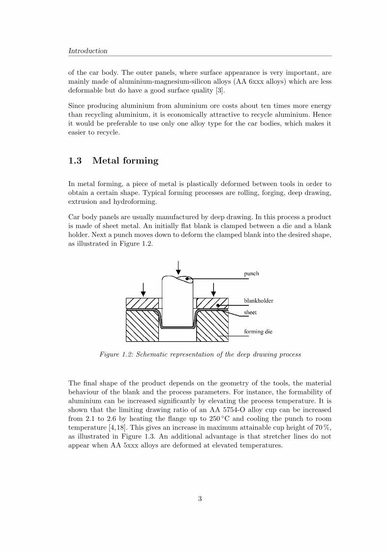
Car body panels are usually manufactured by deep drawing. In this process a productis made of sheet metal. An initially flat blank is clamped between a die and a blankholder. Next a punch moves down to deform the clamped blank into the desired shape,as illustrated in Figure 1.2.
Figure 1.2: Schematic representation of the deep drawing process
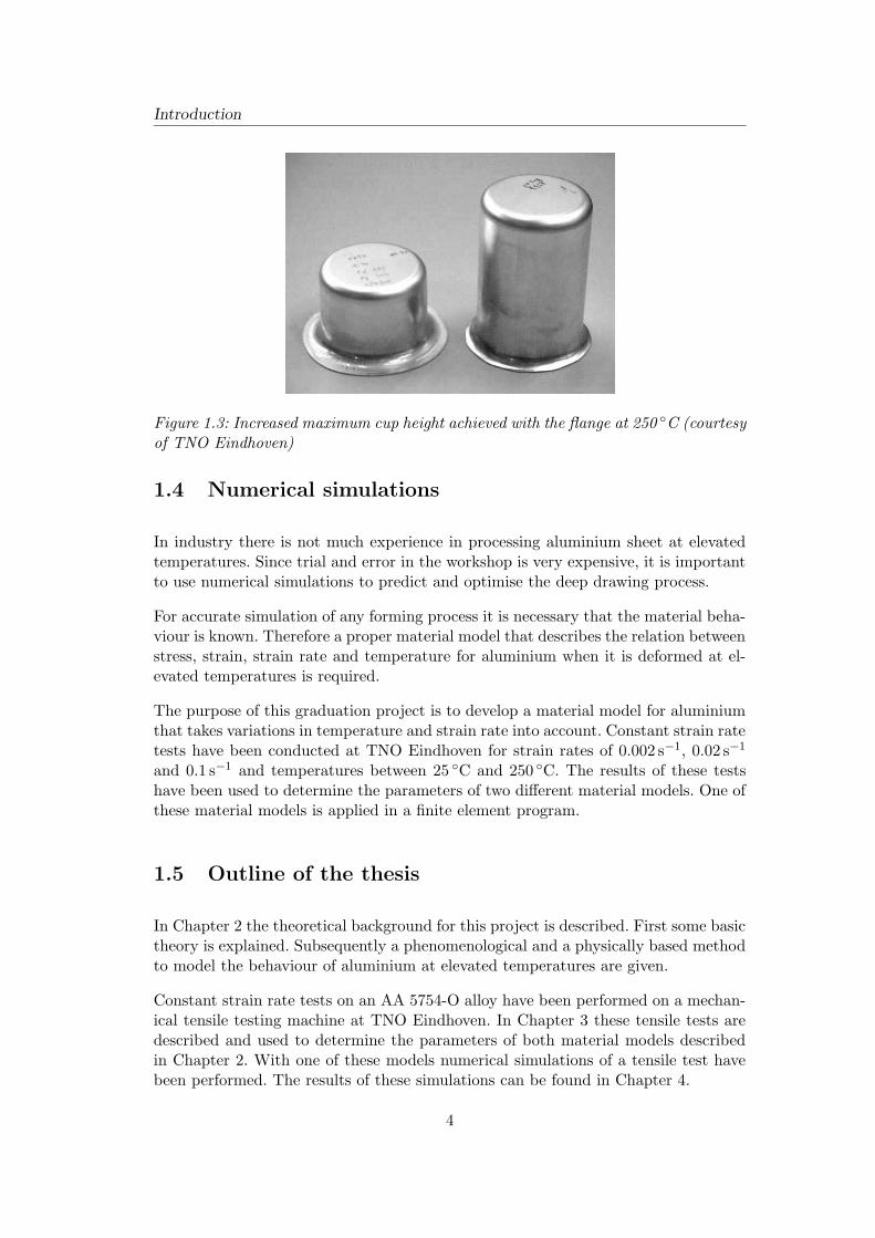
The final shape of the product depends on the geometry of the tools, the materialbehaviour of the blank and the process parameters. For instance, the formability ofaluminium can be increased significantly by elevating the process temperature. It isshown that the limiting drawing ratio of an AA 5754-O alloy cup can be increasedfrom 2.1 to 2.6 by heating the flange up to 250 C and cooling the punch to roomtemperature [4,18]. This gives an increase in maximum attainable cup height of 70%,as illustrated in Figure 1.3. An additional advantage is that stretcher lines do notappear when AA 5xxx alloys are deformed at elevated temperatures.
3
Introduction
Figure 1.3: Increased maximum cup height achieved with the flange at 250 C (courtesyof TNO Eindhoven)
1.4 Numerical simulations
In industry there is not much experience in processing aluminium sheet at elevatedtemperatures. Since trial and error in the workshop is very expensive, it is importantto use numerical simulations to predict and optimise the deep drawing process.
For accurate simulation of any forming process it is necessary that the material beha-viour is known. Therefore a proper material model that describes the relation betweenstress, strain, strain rate and temperature for aluminium when it is deformed at el-evated temperatures is required.
The purpose of this graduation project is to develop a material model for aluminiumthat takes variations in temperature and strain rate into account. Constant strain ratetests have been conducted at TNO Eindhoven for strain rates of 0.002 s−1, 0.02 s−1
and 0.1 s−1 and temperatures between 25 C and 250 C. The results of these testshave been used to determine the parameters of two different material models. One ofthese material models is applied in a finite element program.
1.5 Outline of the thesis
In Chapter 2 the theoretical background for this project is described. First some basictheory is explained. Subsequently a phenomenological and a physically based methodto model the behaviour of aluminium at elevated temperatures are given.
Constant strain rate tests on an AA 5754-O alloy have been performed on a mechan-ical tensile testing machine at TNO Eindhoven. In Chapter 3 these tensile tests aredescribed and used to determine the parameters of both material models describedin Chapter 2. With one of these models numerical simulations of a tensile test havebeen performed. The results of these simulations can be found in Chapter 4.
4

Introduction
To determine which material model describes the behaviour of aluminium duringa rapid change in strain rate (a strain rate jump) at elevated temperatures best,more tensile tests have been performed on a hydraulic tensile testing machine at theUniversity of Twente. In Chapter 5 these uniaxial tensile tests with strain rate jumpsare described.
Finally in Chapter 6 the conclusions from this research are summarised and recom-mendations for future research are presented.
5
Chapter 2
Modelling material behaviour
In this chapter the theory used in this thesis is presented. First the basic relationshipbetween stress and strain is given. Next the influence of temperature and strain rateon this stress-strain relationship is described. Finally both a phenomenological anda physically based material model that are used to model the material behaviour ofaluminium at elevated temperatures are presented.
2.1 Stress and strain
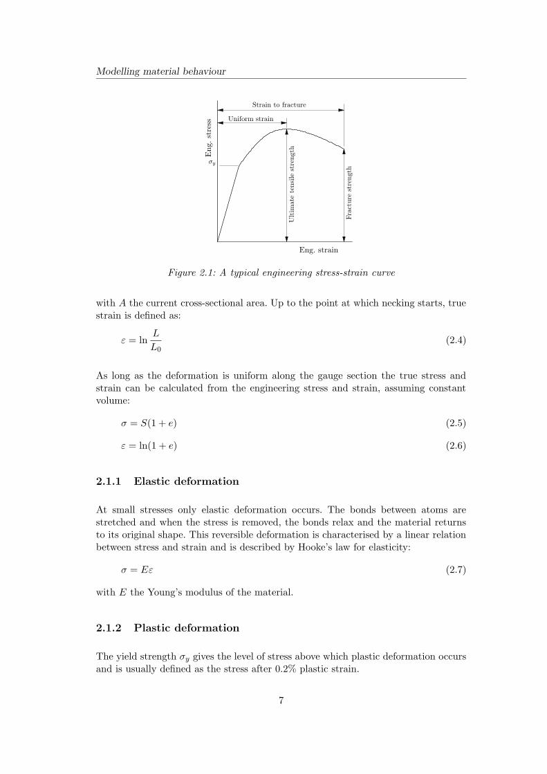
The relationship between stress and strain of a material can be determined in a tensiletest. This is one of the most commonly used tests for evaluating material behaviour.A test specimen is loaded uniaxially, resulting in a gradual elongation and eventuallyfracture of the specimen. The measured tensile force F and displacement ∆L = L−L0
are used to calculate the engineering stress S and the engineering strain e:
S =F
A0(2.1)
e =L− L0
L0(2.2)
with A0 the initial cross-sectional area, L the current length and L0 the initial length.In Figure 2.1 a typical engineering stress-strain curve produced in a uniaxial tensiletest is given.
The engineering stress and strain depend on the initial length and cross-sectionalarea of the specimen. When the results of the tensile tests are used to predict howthe material will behave under other conditions, it is desirable to translate the resultsto the true stress σ and true strain ε. True stress is defined as:
σ =F
A(2.3)
6
Modelling material behaviour
PSfrag replacements
Eng. strain
Eng.
stress
σy
Ultim
atetensile
strength
Fracture
strength
Uniform strain
Strain to fracture
Figure 2.1: A typical engineering stress-strain curve
with A the current cross-sectional area. Up to the point at which necking starts, truestrain is defined as:
ε = lnL
L0(2.4)
As long as the deformation is uniform along the gauge section the true stress andstrain can be calculated from the engineering stress and strain, assuming constantvolume:
σ = S(1 + e) (2.5)
ε = ln(1 + e) (2.6)
2.1.1 Elastic deformation
At small stresses only elastic deformation occurs. The bonds between atoms arestretched and when the stress is removed, the bonds relax and the material returnsto its original shape. This reversible deformation is characterised by a linear relationbetween stress and strain and is described by Hooke’s law for elasticity:
σ = Eε (2.7)
with E the Young’s modulus of the material.
2.1.2 Plastic deformation
The yield strength σy gives the level of stress above which plastic deformation occursand is usually defined as the stress after 0.2% plastic strain.
7
Modelling material behaviour
The flow stress σf denotes the resistance to plastic deformation of a material. Asa ductile material is plastically deformed it becomes harder and stronger, a processknown as strain hardening. Strain hardening can be explained on the basis of in-teractions between dislocations. When a material is being deformed, the dislocationdensity increases. Consequently the average distance between dislocations decreasesand the motion of a dislocation is hindered by the presence of other dislocations.As the dislocation density increases, the resistance to dislocation motion by otherdislocations becomes more pronounced and the stress necessary to deform a metalincreases.
The relation between flow stress and strain is often described by a power law, e.g. theNadai relation:
σf = C1εn (2.8)
with C1 a material constant and n the strain hardening coefficient, which gives anindication of the ability of the sheet to distribute the strain over a wide region [9,12].
2.2 Temperature and strain rate effects
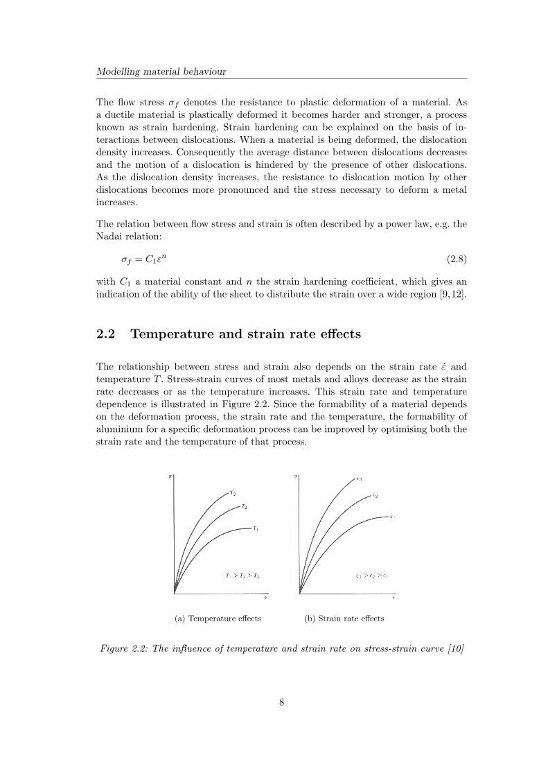
The relationship between stress and strain also depends on the strain rate ε andtemperature T . Stress-strain curves of most metals and alloys decrease as the strainrate decreases or as the temperature increases. This strain rate and temperaturedependence is illustrated in Figure 2.2. Since the formability of a material dependson the deformation process, the strain rate and the temperature, the formability ofaluminium for a specific deformation process can be improved by optimising both thestrain rate and the temperature of that process.
(a) Temperature effects (b) Strain rate effects
Figure 2.2: The influence of temperature and strain rate on stress-strain curve [10]
8
Modelling material behaviour
2.2.1 Temperature effects
The melting temperature of aluminium-magnesium alloys is in the order of 640 C.The homologous temperature Th is defined as the absolute temperature T a dividedby the absolute melting temperature T a
m:
Th =T a
T am
(2.9)
For the temperature range of interest for this research (25 C to 250 C), the homolog-ous temperature ranges from 0.33 to 0.57. At homologous temperatures between 0.3and 0.5, the material strength decreases because of thermally activated processes likecross slip that allow the high local stresses to be relaxed. For higher temperatures, dif-fusion processes become important and mechanisms like recovery and recrystallisationprevent pile-ups and further reduce the strength of the material.
Recovery is the relieve of the build-up of dislocations from strain hardening whencrystal imperfections are rearranged or eliminated into new configurations. For AA5xxx alloys recovery can already start at temperatures as low as 95− 120 C.
Recrystallisation is a rapid restoration process, in which new, dislocation-free crystalsnucleate and grow at the expense of original grains. For AA 5xxx alloys recrystallisa-tion occurs only above 250 C so it is not expected to occur during the tensile testsperformed for this project [5, 9, 12].
2.2.2 Strain rate effects
The relationship between stress and strain rate for a certain strain and temperatureis often described by a power-law of the same form as Equation 2.8:
σ = C2εm (2.10)
with C2 a material constant and m the strain rate sensitivity. For most metals mvaries between 0.02 and 0.2. The strain rate sensitivity increases with increasingtemperatures.
2.2.3 Dynamic strain ageing
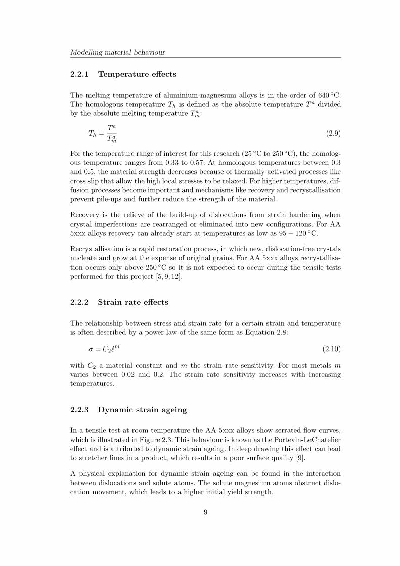
In a tensile test at room temperature the AA 5xxx alloys show serrated flow curves,which is illustrated in Figure 2.3. This behaviour is known as the Portevin-LeChateliereffect and is attributed to dynamic strain ageing. In deep drawing this effect can leadto stretcher lines in a product, which results in a poor surface quality [9].
A physical explanation for dynamic strain ageing can be found in the interactionbetween dislocations and solute atoms. The solute magnesium atoms obstruct dislo-cation movement, which leads to a higher initial yield strength.
9
Modelling material behaviour
Figure 2.3: Serrated flow curve [9]
At low strain rates dislocations move slowly and the solute atoms can migrate to thedislocation while they are arrested at other obstacles or solute atoms. This furtherobstructs dislocation movement and causes a higher flow stress. At higher strainrates the solute atoms cannot migrate to the dislocations, which results in a lowerflow stress. Macroscopically this appears as a negative strain rate sensitivity, whichcan lead to instabilities.
At elevated temperatures the mobility of the solute atoms increases and the serrationsdisappear. Therefore, when forming at elevated temperatures no stretcher lines occur,and the surface quality is good [9, 18].
2.3 Material models
There are several ways to model material behaviour. In this section two models arepresented: a phenomenological and a physically based material model. Both modelsdescribe the flow stress as a function of the deformation path, temperature and strainrate.
2.3.1 A phenomenological model
A phenomenological model is actually the classical approach for modelling materialbehaviour. Macroscopic mechanical test results are fitted to a convenient mathemat-ical function. A good approximation of the stress-strain curve was already given inEquation 2.8. If the material is pre-strained the relationship changes to:
σ = C1(ε+ ε0)n (2.11)
with ε0 the initial strain.
This equation only considers strain hardening. In Section 2.2 it was shown that thestrain rate and temperature also have a significant influence on the stress. The strainrate sensitivity is described in Equation 2.10.
10
Modelling material behaviour
Combining Equations 2.10 and 2.11 gives:
σf = C(ε+ ε0)n
(
ε
ε0
)m
(2.12)
with ε0 a reference strain rate.
The effect of the temperature on the stress is accounted for by assuming that C, nand m are functions of the temperature. The following relations were shown to givegood results [20]:
C(T ) = C0 + a1
[
1− exp
(
a2T − 273
Tm
)]
(2.13)
n(T ) = n0 + b1
[
1− exp
(
b2T − 273
Tm
)]
(2.14)
m(T ) = m0 exp
(
cT − 273
Tm
)
(2.15)
with C0, a1, a2, n0, b1, b2, m0 and c material constants and Tm a reference temperat-ure. From now on this model will be referred to as the extended Nadai model [18–20].
2.3.2 A physically based material model
A physically based model predicts the relationship between stress and strain byconsidering the physical mechanisms of plastic deformation. The physically basedmodel used here was first described by Bergstrom [1,2] and has been adapted by VanLiempt [21]. The deformation resistance of metals is divided into three parts:
σf = σo(T ) + σw(ρ, T ) + σ∗(ε, T ) (2.16)
with σ0 the strain rate independent stress, σw the contribution of the strain hardeningand σ∗ a dynamic stress that depends on the strain rate and temperature.
Dynamic stress
The dynamic stress σ∗ is often defined by a relation attributed to Krabiell and Dahl[11]:
σ∗(ε, T ) = σ∗0
1 +kT
∆G0ln( ε
ε0
)
for ε0 exp(
− ∆G0
kT
)
< ε < ε0
(2.17)
with σ∗0 a maximum value for the dynamic stress, k the Boltzmann’s constant and∆G0 the activation energy.
11
Modelling material behaviour
The preliminary results of the tensile tests performed at TNO Eindhoven show thatthe influence on the initial yield stress is small at low temperatures and increasesrapidly at higher temperatures [19, 20]. However, Equation 2.17 gives a high strainrate influence at low temperatures that decreases at high temperatures. Since this isin contradiction to the experimental results, the dynamic stress neglected.
Strain hardening
For the contribution of strain hardening σw, a simple one-parameter model is usedwhere the evolution of the dislocation density ρ is responsible for the hardening. Therelation between the dislocation density and the strain hardening is given by theTaylor equation:
σw = αG(T )b√ρ (2.18)
with α a scaling parameter, G the elastic shear modulus and b the Burgers vector [18].
The essential part of Equation 2.18 is the evolution of the dislocation density. Thisgives the influence of temperature and strain rate on the hardening. It is formulatedas an evolution equation:
dρ
dε= U(ρ)− Ω(ε, T )ρ (2.19)
with U the immobilisation rate of dislocations and Ω the remobilisation rate of dis-locations:
U = U0√ρ (2.20)
Ω = Ω0 + C3exp(
− mQv
RT
)
ε−m (2.21)
with U0 the intrinsic immobilisation rate, Ω0 the low temperature, high strain ratelimit value of the remobilisation probability, C3 and m constants, Qv the activationenergy and R the gas constant.
Equation 2.19 can be integrated analytically for constant U0 and Ω [8, 21]. For anincremental algorithm, the dislocation density ρi+1 at time ti+1 can be calculatedfrom:
ρi+1 =
[
U0
Ω
(
exp(12Ω∆ε)− 1
)
+√ρi
]2
exp(−Ω∆ε) (2.22)
where U0 and Ω are assumed to be constant during the time increment. This gives acontribution to the flow stress of:
σwi+1 = αGb
√ρi+1 (2.23)
which leads to:
σwi+1 = αGb
[
(U0
Ω−√ρi
)(
1− exp(−12Ω∆ε)
)
+√ρi
]
(2.24)
12
Modelling material behaviour
Strain rate independent stress
The strain rate independent stress σ0 is assumed to relate to stresses in the atomiclattice. Therefore the temperature dependence of the shear modulus G(T ) is also usedfor the strain rate independent stress [16, 18].
Bergstrom model
Combining Equation 2.16 with the information described above results in:
σf = g(T )(
σ0 + αGrefb√ρ)
(2.25)
with g(T ) the shear modulus divided by the reference value Gref . In this work thetemperature dependence is numerically represented by the empirical relation:
g(T ) = 1− CT exp
(
− T1
T
)
(2.26)
with CT and T1 fitting parameters. From now on this model will be referred to as theBergstrom model.
13
Chapter 3
Experiments at constant strain
rate
Constant strain rate tensile tests have been performed at TNO Eindhoven. In thischapter these tests and the results are first described. After this the parameters ofthe material models described in Chapter 2 are determined using these tensile testresults. The objective is to predict the behaviour of aluminium-magnesium alloys whendeformed at elevated temperatures.
3.1 Tensile testing at TNO Eindhoven
In this section the tensile tests that were performed at TNO Eindhoven are described.First the characteristics of the tested material and the experimental test set-up arediscussed. Subsequently the results of the performed tensile tests are given.
3.1.1 Material characteristics of 5754-O
In this thesis, the AA 5754-O alloy is used for the experiments as a representativeexample of the 5xxx alloys. The chemical composition of this alloy, as given by themanufacturer, is presented in Table 3.1. The main alloying element is magnesium,which has a strengthening effect on the aluminium. Since the solid solubility of thisalloying element is higher than 10%, it is in solid solution and the alloy constitutesof a single phase. This means that the original crystal structure of the aluminium ismaintained. The mean grain size of the alloy is 20− 25µm.
The AA 5754-O alloy is in a fully annealed state. Therefore the test results are notinfluenced by the time that a specimen is kept at elevated temperatures prior todeformation.
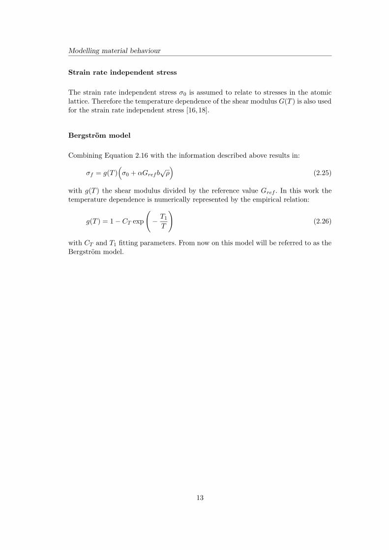
The test specimens were manufactured according to EN-10002 Form 1, as illustrated
14
Experiments at constant strain rate
Table 3.1: The chemical composition of the AA 5754-O alloy
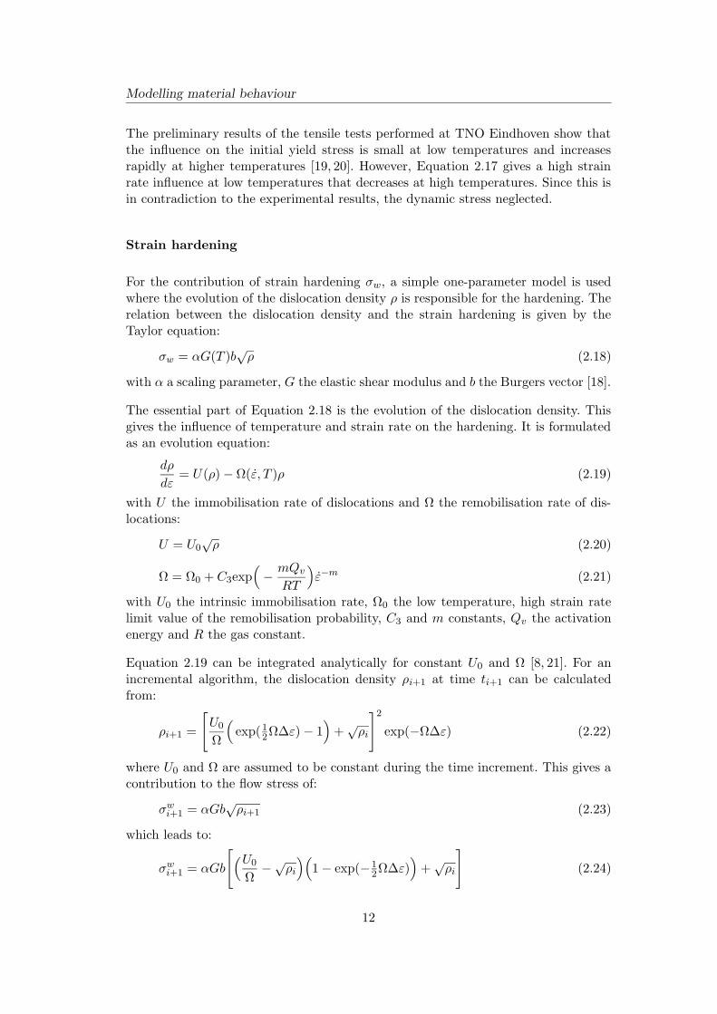
Alloying element %
Magnesium 3.356Manganese 0.320Silicon 0.130Copper 0.010Titanium 0.009Aluminium Remainder
in Figure 3.1. They were made from a single batch of sheet material with a thicknessof 1.2mm. The tensile direction is perpendicular to the rolling direction of the sheetmaterial. The elongation of the specimen during testing is measured directly over aninitial length of 50mm.
75
12.5
20
20
> 35
Figure 3.1: Tensile test specimen according to EN-10002 Form 1 (dimensions in mm)
3.1.2 Experimental set-up
All tests were performed on a Zwick mechanical tensile tester. Prior to testing thespecimen and clamps were placed in a furnace. The furnace was heated to the desiredtemperature, after which the specimen was clamped on one side. After re-heating thefurnace, the other side was clamped. The test was started when the desired testingtemperature was reached again. Depending on the required temperature, it took aboutone to three minutes before the specimen was clamped properly and the test couldbe started. The temperature in the furnace was controlled by a PID controller within1 C.
3.1.3 Tensile test results
Tensile tests at a constant strain rate and constant temperature were conducted atvarious strain rates (0.002 s−1, 0.02 s−1 and 0.1 s−1) and temperatures (between roomtemperature and 250 C). Per strain rate and temperature, two to five tests havebeen performed. The experiments were conducted over a time-span of one year, butno systematic difference between test results was found.
15
Experiments at constant strain rate
0
50
100
150
200
250
0 0.1 0.2 0.3 0.4 0.5 0.6 0.7 0.8 0.9 1
PSfrag replacements
Engineering strain (-)
Engineeringstress
(MPa)
T = 25 CT = 100 CT = 125 CT = 150 CT = 175 CT = 200 CT = 225 CT = 250 C
(a) ε =0.002s−1
0
50
100
150
200
250
0 0.1 0.2 0.3 0.4 0.5 0.6 0.7 0.8 0.9 1
PSfrag replacements
Engineering strain (-)
Engineeringstress
(MPa)
T = 25 CT = 100 CT = 125 CT = 150 CT = 175 CT = 200 CT = 225 CT = 250 C
(b) ε =0.02s−1
0
50
100
150
200
250
0 0.1 0.2 0.3 0.4 0.5 0.6 0.7 0.8 0.9 1
PSfrag replacements
Engineering strain (-)
Engineeringstress
(MPa)
T = 25 C
T = 100 CT = 125 CT = 150 C T = 175 C
T = 200 C
T = 225 C
T = 250 C
(c) ε =0.1s−1
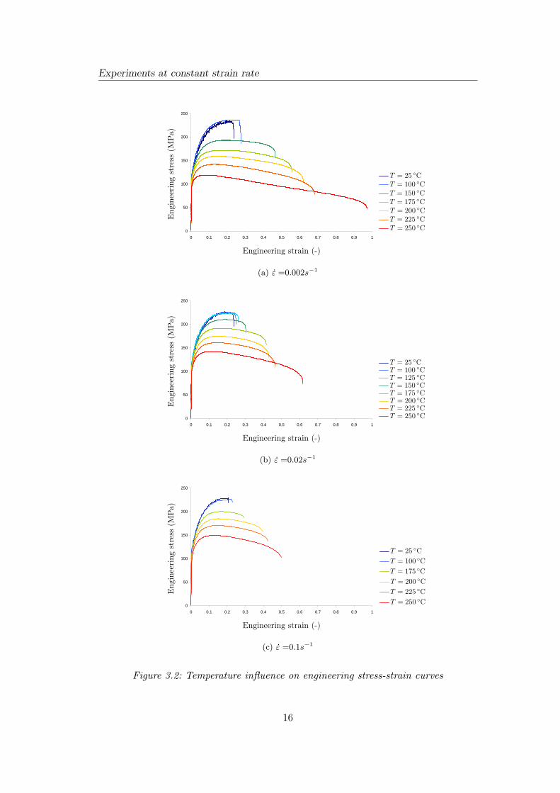
Figure 3.2: Temperature influence on engineering stress-strain curves
16
Experiments at constant strain rate
In Figure 3.2 the temperature influence on the engineering stress-strain curves can beseen. Only one representative result per specific test is given. The stress-strain curvesat relatively low temperatures show the serrations that cause the stretcher lines, asexplained in Section 2.2.3. Figure 3.2(b) shows that for temperatures above 125 Cthese serrations no longer occur. For all strain rates there is hardly any differencebetween the stress-strain curves at room temperature and at 100 C. When the testtemperature exceeds 125 C, the ultimate tensile strength decreases with increasingtemperature.
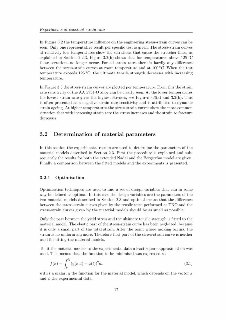
In Figure 3.3 the stress-strain curves are plotted per temperature. From this the strainrate sensitivity of the AA 5754-O alloy can be clearly seen. At the lower temperaturesthe lowest strain rate gives the highest stresses, see Figures 3.3(a) and 3.3(b). Thisis often presented as a negative strain rate sensitivity and is attributed to dynamicstrain ageing. At higher temperatures the stress-strain curves show the more commonsituation that with increasing strain rate the stress increases and the strain to fracturedecreases.
3.2 Determination of material parameters
In this section the experimental results are used to determine the parameters of thematerial models described in Section 2.3. First the procedure is explained and sub-sequently the results for both the extended Nadai and the Bergstrom model are given.Finally a comparison between the fitted models and the experiments is presented.
3.2.1 Optimisation
Optimisation techniques are used to find a set of design variables that can in someway be defined as optimal. In this case the design variables are the parameters of thetwo material models described in Section 2.3 and optimal means that the differencebetween the stress-strain curves given by the tensile tests performed at TNO and thestress-strain curves given by the material models should be as small as possible.
Only the part between the yield stress and the ultimate tensile strength is fitted to thematerial model. The elastic part of the stress-strain curve has been neglected, becauseit is only a small part of the total strain. After the point where necking occurs, thestrain is no uniform anymore. Therefore that part of the stress-strain curve is neitherused for fitting the material models.
To fit the material models to the experimental data a least square approximation wasused. This means that the function to be minimised was expressed as:
f(x) =
∫ t2
t1
(y(x, t)− φ(t))2dt (3.1)
with t a scalar, y the function for the material model, which depends on the vector xand φ the experimental data.
17
Experim
ents
at
consta
nt
strain
rate
0
50
100
150
200
250
0.0 0.2 0.4 0.6 0.8 1.0
PSfrag replacements
Engineering strain (-)
Engineeringstress
(MPa)
ε = 0.002 s−1
ε = 0.02 s−1
ε = 0.1 s−1
(a) T = 25C
0
50
100
150
200
250
0.0 0.2 0.4 0.6 0.8 1.0
PSfrag replacements
Engineering strain (-)
Engineeringstress
(MPa)
ε = 0.002 s−1
ε = 0.02 s−1
ε = 0.1 s−1
(b) T = 100C
0
50
100
150
200
250
0.0 0.2 0.4 0.6 0.8 1.0
PSfrag replacements
Engineering strain (-)
Engineeringstress
(MPa)
ε = 0.002 s−1
ε = 0.02 s−1
ε = 0.1 s−1
(c) T = 175C
0
50
100
150
200
250
0.0 0.2 0.4 0.6 0.8 1.0
PSfrag replacements
Engineering strain (-)Engineeringstress
(MPa)
ε = 0.002 s−1
ε = 0.02 s−1
ε = 0.1 s−1
(d) T = 250C
Figure 3.3: Strain rate influence on engineering stress-strain curves
18
Experiments at constant strain rate
PSfrag replacements
Design variable 1
Designvariab
le2
Figure 3.4: A simplex in 2 dimensions
For the minimising of this function an unconstrained minimisation technique wasused: the simplex search of Nelder and Mead [14]. This is a direct search method thatonly uses function evaluations without applying numerical or analytical gradients.
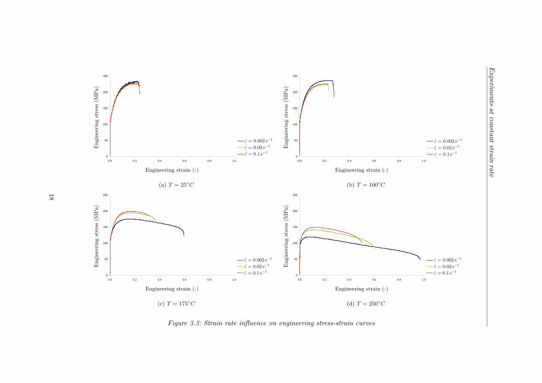
Simplex search methods are based on an initial design of n+1 trials, where n isthe number of variables. A simplex is an n+1 geometric figure in an n-dimensionalspace. In Figure 3.4 a simplex in a 2-dimensional space is given, hence the simplexis a triangle. The corners of the geometric figure are called vertices and the simplexsearch method evaluates the function at each vertex. It then decides which is the worstvalue and mirrors that vertex through the centroid of the remaining n vertices, thusforming a new simplex. The Nelder-Mead simplex search method has the additionaladvantage that it can adjust its shape and size depending on the response in eachstep. Therefore it is possible to accelerate the optimisation process.
Prior to fitting, the experimental data set was reduced to twelve stress-strain curves,each composed of 21 data points. Each stress-strain curve represents a single combin-ation of the following temperatures and strain rates: 25 C, 100 C, 175 C and 250 Cand 0.002 s−1, 0.02 s−1 and 0.1 s−1.
3.2.2 Extended Nadai model
The extended Nadai model has been described in Section 2.3.1. The parameters Tm
and ε0 are used to scale parts of the equations, resulting in dimensionless expressions,and can be chosen arbitrarily. The remaining nine parameters were simultaneouslyfitted to the selected uniaxial tensile tests. In Table 3.2 the results of this fit aregiven. The standard deviation of the difference between the experimental results andthe results given by the extended Nadai model, the so-called RMS error value, is5.56MPa.
19
Experiments at constant strain rate
Table 3.2: Parameters for the extended Nadai model
Tm 800K a1 109.7MPa n0 0.3212ε0 0.004603 a2 3.965 m0 0.001625ε0 0.002 s−1 b1 0.2389 c 10.23C0 488.0MPa b2 1.463
3.2.3 Bergstrom model
The Bergstrom model was described in Section 2.3.2. Some of the parameters in thismodel can be selected beforehand. The initial dislocation density ρ0 was chosen to be1011 m−2, which is a reasonable value for annealed aluminium. The magnitude of theBurgers vector b and the shear modulus at room temperature Gref were taken fromliterature. Furthermore the scaling factor α was chosen to be 1.
The eight remaining parameters were fitted to the same tensile tests that were usedto fit the extended Nadai model. In Table 3.3 the resulting values are presented.The RMS error value between the experimental results and the Bergstrom model is3.76MPa.
Table 3.3: Parameters for the Bergstrom model
σ0 103.7MPa m 0.3456 ρ0 1011 m−2
α 1.0 U0 6.331· 108 m−1 Gref 26354MPab 2.857· 10−10 m Ω0 25.35 CT 123.4C 3.232· 105 Qv 1.287· 105 J/mol T1 3639K
3.2.4 Comparison of the models
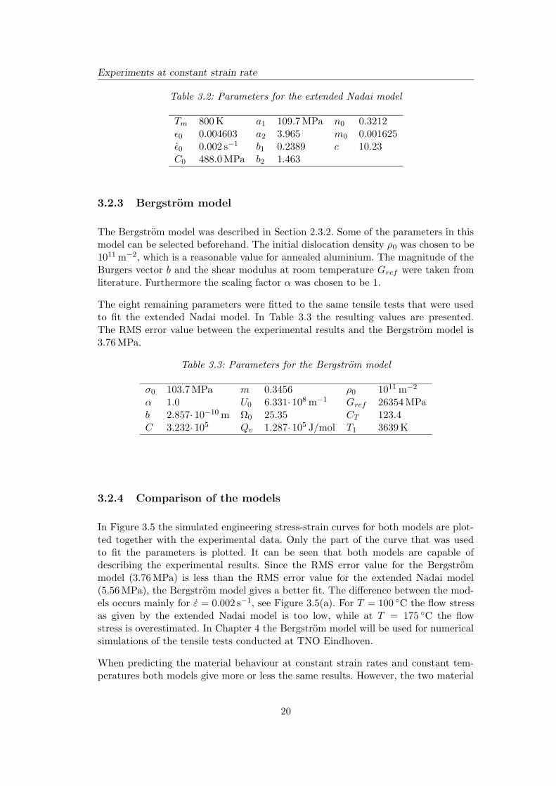
In Figure 3.5 the simulated engineering stress-strain curves for both models are plot-ted together with the experimental data. Only the part of the curve that was usedto fit the parameters is plotted. It can be seen that both models are capable ofdescribing the experimental results. Since the RMS error value for the Bergstrommodel (3.76MPa) is less than the RMS error value for the extended Nadai model(5.56MPa), the Bergstrom model gives a better fit. The difference between the mod-els occurs mainly for ε = 0.002 s−1, see Figure 3.5(a). For T = 100 C the flow stressas given by the extended Nadai model is too low, while at T = 175 C the flowstress is overestimated. In Chapter 4 the Bergstrom model will be used for numericalsimulations of the tensile tests conducted at TNO Eindhoven.
When predicting the material behaviour at constant strain rates and constant tem-peratures both models give more or less the same results. However, the two material
20
Experiments at constant strain rate
0
50
100
150
200
250
0 0.05 0.1 0.15 0.2 0.25
PSfrag replacements
Engineering strain (-)
Engineeringstress
(MPa)
e, T = 25 Cn, T = 25 Cb, T = 25 Ce, T = 100 Cn, T = 100 Cb, T = 100 Ce, T = 175 Cn, T = 175 Cb, T = 175 Ce, T = 250 Cn, T = 250 Cb, T = 250 C
(a) ε =0.002s−1
0
50
100
150
200
250
0 0.05 0.1 0.15 0.2 0.25
PSfrag replacements
Engineering strain (-)
Engineeringstress
(MPa)
e, T = 25 Cn, T = 25 Cb, T = 25 Ce, T = 100 Cn, T = 100 Cb, T = 100 Ce, T = 175 Cn, T = 175 Cb, T = 175 Ce, T = 250 Cn, T = 250 Cb, T = 250 C
(b) ε =0.02s−1
0
50
100
150
200
250
0 0.05 0.1 0.15 0.2 0.25
PSfrag replacements
Engineering strain (-)
Engineeringstress
(MPa)
e, T = 25 Cn, T = 25 Cb, T = 25 Ce, T = 100 Cn, T = 100 Cb, T = 100 Ce, T = 175 Cn, T = 175 Cb, T = 175 Ce, T = 250 Cn, T = 250 Cb, T = 250 C
(c) ε =0.1s−1
Figure 3.5: Engineering stress-strain curves for e = experiments, n = extended Nadaimodel and b = Bergstrom model
21
Experiments at constant strain rate
0
50
100
150
200
250
0.00 0.05 0.10 0.15
PSfrag replacements
Engineering strain (-)
Engineeringstress
(MPa)
T = 175 C, ε = 0.002 s−1
T = 175 C, ε = 0.02 s−1
T = 175 C, ε = 0.002− 0.02 s−1
T = 175 C, ε = 0.02− 0.002 s−1T = 250 C, ε = 0.002 s−1
T = 250 C, ε = 0.02 s−1 T = 250 C, ε = 0.002− 0.02 s−1
T = 250 C, ε = 0.02− 0.002 s−1
(a) Extended Nadai model
0
50
100
150
200
250
0.00 0.05 0.10 0.15
PSfrag replacements
Engineering strain (-)
Engineeringstress
(MPa)
T = 175 C, ε = 0.002 s−1
T = 175 C, ε = 0.02 s−1
T = 175 C, ε = 0.002− 0.02 s−1
T = 175 C, ε = 0.02− 0.002 s−1
T = 250 C, ε = 0.002 s−1
T = 250 C, ε = 0.02 s−1
T = 250 C, ε = 0.002− 0.02 s−1
T = 250 C, ε = 0.02− 0.002 s−1
(b) Bergstrom model
Figure 3.6: Engineering stress-strain curves with and without strain rate jumps
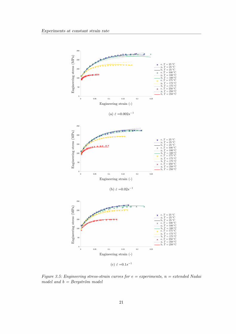
models give completely different predictions when a jump in the strain rate is simu-lated. A jump in strain rate can be applied by altering the strain rate instantaneousat a certain strain. In Figure 3.6 stress-strain curves are plotted for deformation at175 C and 250 C with strain rates 0.002 s−1 and 0.02 s−1. Strain rate changes from0.002 s−1 to 0.02 s−1 or vice versa are applied after a strain of 0.05. It can be seenthat the extended Nadai model immediately follows the curve of the other constantstrain rate curve. The Bergstrom model only slowly approaches the other constantstrain rate curve. To verify which of the two models predicts the material behaviourbest, tests at constant temperature with strain rate jumps were performed at theUniversity of Twente. In Chapter 5 these experiments and the results are described.
22
Chapter 4
Finite element simulations
In this chapter the applicability of the Bergstrom model is demonstrated by numericalsimulations of uniaxial tensile tests. The finite element program used for the numericalsimulations described in this chapter is called DiekA. This program is being developedat the University of Twente and is specifically designed to simulate forming processes.
4.1 Simulating tensile tests
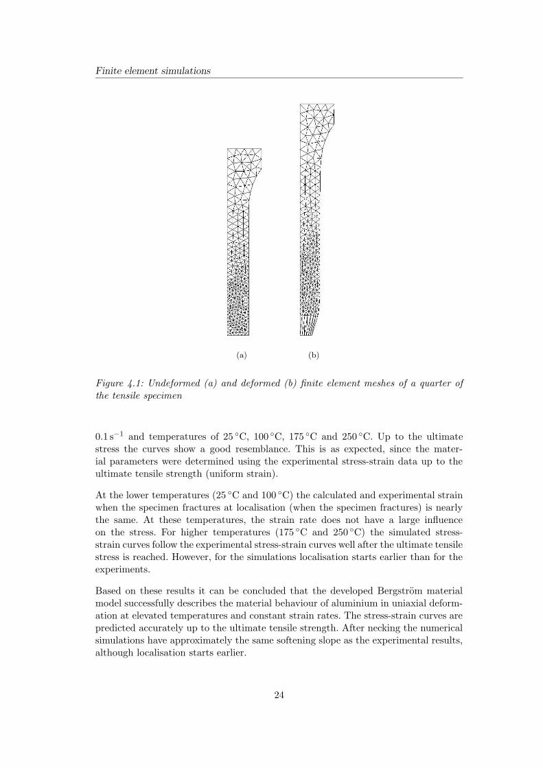
The Bergstrom material model with the parameters as derived in Section 3.2.3 isapplied in numerical simulations. The tensile test specimens used in the tensile testsperformed at TNO Eindhoven, as described in Section 3.1.1, are modelled and meshedin the finite element program DiekA, see Figure 4.1(a). As the clamping area of thespecimen is also modelled, a slight non-uniform strain distribution occurs which res-ults in necking at the centre of the specimen, without prescribing an initial imperfec-tion. In contrast to low temperatures, at elevated temperatures the tensile specimennecks perpendicular to the tensile direction. This results in a symmetric situation.Therefore it is only necessary to model a quarter section of the specimen and thenspecify symmetric conditions.
In order to describe necking accurately, the mesh is refined at the centre area. Thesmallest elements have a size of approximately 1mm, which is of the same order asthe sheet thickness. This necking can be seen in Figure 4.1(b) where a deformed meshis given.
4.2 Results
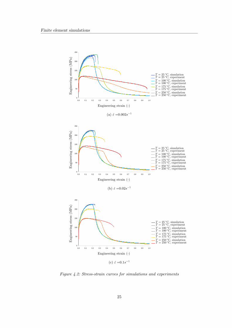
Equivalent with the experimental results, the numerical stress-strain curves were de-termined for a gauge length of 50mm. In Figure 4.2 both the numerical and exper-imental stress-strain curves are presented for strain rates of 0.002 s−1, 0.02 s−1 and
23
Finite element simulations
(a) (b)
Figure 4.1: Undeformed (a) and deformed (b) finite element meshes of a quarter ofthe tensile specimen
0.1 s−1 and temperatures of 25 C, 100 C, 175 C and 250 C. Up to the ultimatestress the curves show a good resemblance. This is as expected, since the mater-ial parameters were determined using the experimental stress-strain data up to theultimate tensile strength (uniform strain).
At the lower temperatures (25 C and 100 C) the calculated and experimental strainwhen the specimen fractures at localisation (when the specimen fractures) is nearlythe same. At these temperatures, the strain rate does not have a large influenceon the stress. For higher temperatures (175 C and 250 C) the simulated stress-strain curves follow the experimental stress-strain curves well after the ultimate tensilestress is reached. However, for the simulations localisation starts earlier than for theexperiments.
Based on these results it can be concluded that the developed Bergstrom materialmodel successfully describes the material behaviour of aluminium in uniaxial deform-ation at elevated temperatures and constant strain rates. The stress-strain curves arepredicted accurately up to the ultimate tensile strength. After necking the numericalsimulations have approximately the same softening slope as the experimental results,although localisation starts earlier.
24
Finite element simulations
0
50
100
150
200
250
0.0 0.1 0.2 0.3 0.4 0.5 0.6 0.7 0.8 0.9 1.0
PSfrag replacements
Engineering strain (-)
Engineeringstress
(MPa)
T = 25 C, simulationT = 25 C, experimentT = 100 C, simulationT = 100 C, experimentT = 175 C, simulationT = 175 C, experimentT = 250 C, simulationT = 250 C, experiment
(a) ε =0.002s−1
0
50
100
150
200
250
0.0 0.1 0.2 0.3 0.4 0.5 0.6 0.7 0.8 0.9 1.0
PSfrag replacements
Engineering strain (-)
Engineeringstress
(MPa)
T = 25 C, simulationT = 25 C, experimentT = 100 C, simulationT = 100 C, experimentT = 175 C, simulationT = 175 C, experimentT = 250 C, simulationT = 250 C, experiment
(b) ε =0.02s−1
0
50
100
150
200
250
0.0 0.1 0.2 0.3 0.4 0.5 0.6 0.7 0.8 0.9 1.0
PSfrag replacements
Engineering strain (-)
Engineeringstress
(MPa)
T = 25 C, simulationT = 25 C, experimentT = 100 C, simulationT = 100 C, experimentT = 175 C, simulationT = 175 C, experimentT = 250 C, simulationT = 250 C, experiment
(c) ε =0.1s−1
Figure 4.2: Stress-strain curves for simulations and experiments
25

Finite element simulations
In industrial applications, the strain rate is hardly ever constant. Therefore it isimportant to verify whether the material model describes the material behaviourcorrectly when a strain rate jump is applied. This verification is described in detailin Chapter 5.
26
Chapter 5
Experiments with a strain rate
jump
Both material models described in Chapter 3 predict the material behaviour of alu-minium at elevated temperatures and constant strain rates quite well. However thereis a significant difference in the prediction of the material behaviour of both models incase a strain rate jump is applied. To verify which of the two models describes sucha rapid change in strain rate correct, tensile tests with strain rate jumps at temperat-ures of 175 C and 250 C have been performed at the University of Twente. In thischapter the procedure and the results of these tests are described.
5.1 Experimental set-up
In this section the experimental test set-up of the experiments carried out at theUniversity of Twente is first presented. Subsequently, the procedure to obtain theengineering stress and strain form the data-output is described.
5.1.1 Tensile test equipment
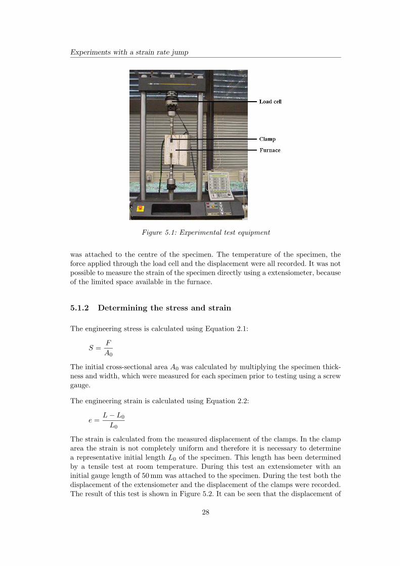
The tensile tests have been carried out on an Instron Model 8516 Testing System,which is a servo-hydraulic tensile testing system. The main advantage of this system,versus the mechanical system used at TNO, is that higher strain rates (over ε =0.2 s−1) and faster strain rate jumps (from ε = 0.002 s−1 to ε = 0.02 s−1 within 0.1 s)are possible. In Figure 5.1 the used tensile test equipment is illustrated.
In these tensile tests the same aluminium-magnesium alloy (AA 5754-O) and speci-mens as applied in the TNO tests were used. To heat the specimens a tubular shapedfurnace was used. Because it has a diameter of only 30 mm, special clamps were de-signed. To measure the temperature of the specimen during the test, a thermocouple
27
Experiments with a strain rate jump
Figure 5.1: Experimental test equipment
was attached to the centre of the specimen. The temperature of the specimen, theforce applied through the load cell and the displacement were all recorded. It was notpossible to measure the strain of the specimen directly using a extensiometer, becauseof the limited space available in the furnace.
5.1.2 Determining the stress and strain
The engineering stress is calculated using Equation 2.1:
S =F
A0
The initial cross-sectional area A0 was calculated by multiplying the specimen thick-ness and width, which were measured for each specimen prior to testing using a screwgauge.
The engineering strain is calculated using Equation 2.2:
e =L− L0
L0
The strain is calculated from the measured displacement of the clamps. In the clamparea the strain is not completely uniform and therefore it is necessary to determinea representative initial length L0 of the specimen. This length has been determinedby a tensile test at room temperature. During this test an extensiometer with aninitial gauge length of 50mm was attached to the specimen. During the test both thedisplacement of the extensiometer and the displacement of the clamps were recorded.The result of this test is shown in Figure 5.2. It can be seen that the displacement of
28
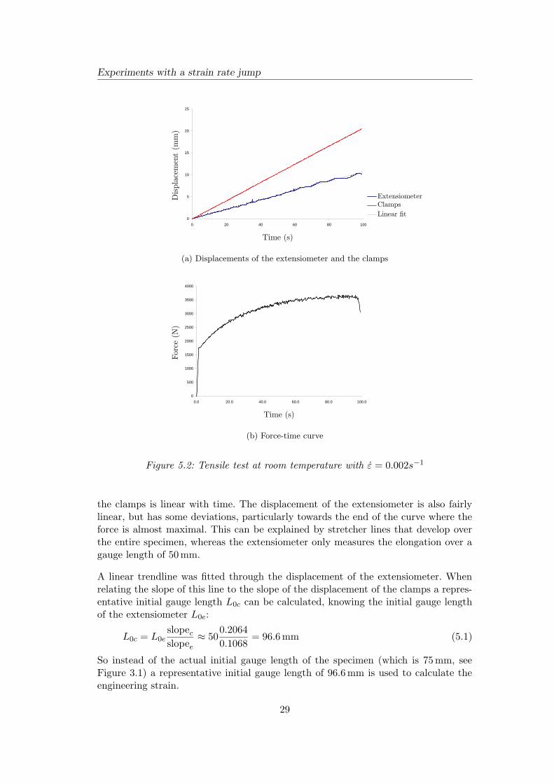
Experiments with a strain rate jump
0
5
10
15
20
25
0 20 40 60 80 100
PSfrag replacements
Time (s)
Displacement(m
m)
ExtensiometerClamps
Linear fit
(a) Displacements of the extensiometer and the clamps
0
500
1000
1500
2000
2500
3000
3500
4000
0.0 20.0 40.0 60.0 80.0 100.0
PSfrag replacements
Time (s)
Force
(N)
(b) Force-time curve
Figure 5.2: Tensile test at room temperature with ε = 0.002s−1
the clamps is linear with time. The displacement of the extensiometer is also fairlylinear, but has some deviations, particularly towards the end of the curve where theforce is almost maximal. This can be explained by stretcher lines that develop overthe entire specimen, whereas the extensiometer only measures the elongation over agauge length of 50mm.
A linear trendline was fitted through the displacement of the extensiometer. Whenrelating the slope of this line to the slope of the displacement of the clamps a repres-entative initial gauge length L0c can be calculated, knowing the initial gauge lengthof the extensiometer L0e:
L0c = L0eslopec
slopee
≈ 500.2064
0.1068= 96.6mm (5.1)
So instead of the actual initial gauge length of the specimen (which is 75mm, seeFigure 3.1) a representative initial gauge length of 96.6mm is used to calculate theengineering strain.
29
Experiments with a strain rate jump
5.2 Verification of the tensile tests
When conducting tensile tests it is important to know all factors that could influencethe test results, like the test equipment used, the temperature distribution in thespecimen and the heating of the specimen due to plastic deformation. In this sectionthese factors are discussed.
5.2.1 Constant strain rate tensile tests
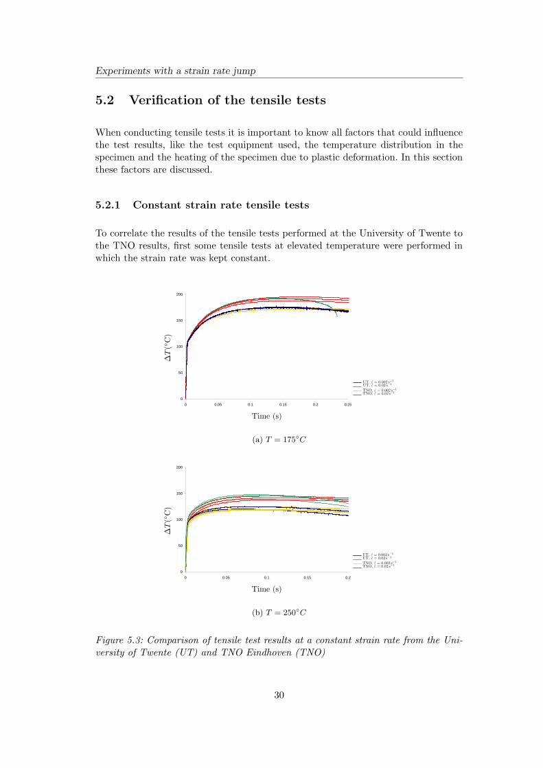
To correlate the results of the tensile tests performed at the University of Twente tothe TNO results, first some tensile tests at elevated temperature were performed inwhich the strain rate was kept constant.
0
50
100
150
200
0 0.05 0.1 0.15 0.2 0.25
PSfrag replacements
Time (s)
∆T(C)
UT, ε = 0.002 s−1
UT, ε = 0.02 s−1
TNO, ε = 0.002 s−1
TNO, ε = 0.02 s−1
(a) T = 175C
0
50
100
150
200
0 0.05 0.1 0.15 0.2
PSfrag replacements
Time (s)
∆T(C)
UT, ε = 0.002 s−1
UT, ε = 0.02 s−1
TNO, ε = 0.002 s−1
TNO, ε = 0.02 s−1
(b) T = 250C
Figure 5.3: Comparison of tensile test results at a constant strain rate from the Uni-versity of Twente (UT) and TNO Eindhoven (TNO)
30

Experiments with a strain rate jump
In Figure 5.3 the results of these tests performed at the University of Twente arecompared to the results of the tensile tests performed at TNO Eindhoven. It can beseen that for ε = 0.002 s−1 the results are quite similar up to uniform strain. Since thedisplacement of the specimen was not measured with the same initial gauge length,after uniform strain the results tests are not comparable anymore. For ε = 0.02 s−1
there is a larger difference between the stress-strain curves of the University of Twenteand TNO. However, keeping in mind that the tests were performed on different tensiletesters and individual tests also show a relatively large spread, these differences areacceptable.
5.2.2 Heating of a specimen
Prior to testing, the specimen is clamped in the tensile tester and the furnace isclosed and turned on. It takes about 30 minutes before the specimen reaches a moreor less steady state temperature of 175 C or 250 C. Since the furnace can only beturned on or off it is difficult to reach this testing temperature accurately. Thereforea temperature of 2-3 C higher than the testing temperature was reached and the testwas started when the specimen had cooled down to the testing temperature.
To verify whether the specimen is heated homogeneously in the furnace, tests havebeen performed with three thermocouples attached to the specimen, one in the centreand one at each end of the gauge. In Figure 5.4 the results for such a test are presented.In this case the specimen was heated to 250 C, for tests where the specimen washeated to 175 C similar results were obtained. When the furnace is turned on thespecimen temperature rises. In Figure 5.4 it can be clearly seen that during theheating sequence the furnace was turned on and off six times. When the thermocoupleattached to the centre of the specimen has reached the testing temperature, the tensiletest is started. It can be seen that at this time (t ≈ 1700 s) the upper thermocouplehas approached approximately the same temperature. However the temperature ofthe lower thermocouple is about 18 C lower. This difference in temperature can
0
50
100
150
200
250
300
0 200 400 600 800 1000 1200 1400 1600 1800
PSfrag replacements
Time (s)
Tem
perature
(C)
Upper thermocouple
Centre thermocouple
Lower thermocouple
Figure 5.4: Heating of a specimen up to 250 C
31
Experiments with a strain rate jump
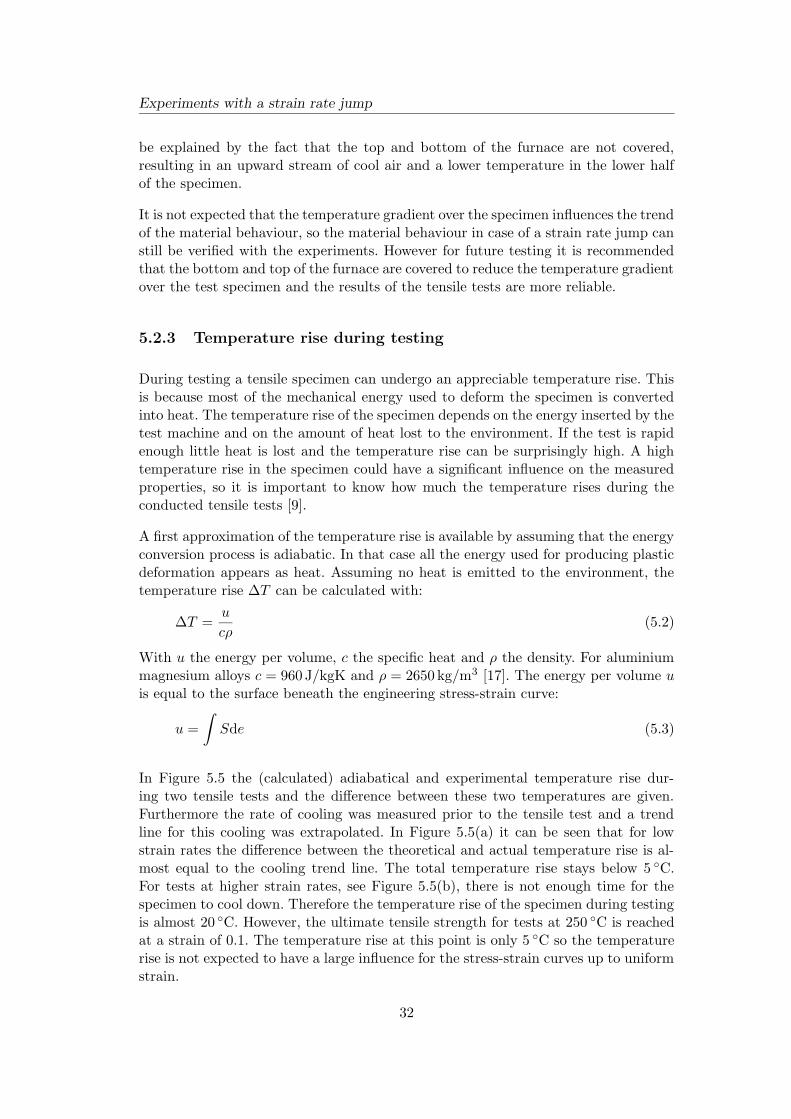
be explained by the fact that the top and bottom of the furnace are not covered,resulting in an upward stream of cool air and a lower temperature in the lower halfof the specimen.
It is not expected that the temperature gradient over the specimen influences the trendof the material behaviour, so the material behaviour in case of a strain rate jump canstill be verified with the experiments. However for future testing it is recommendedthat the bottom and top of the furnace are covered to reduce the temperature gradientover the test specimen and the results of the tensile tests are more reliable.
5.2.3 Temperature rise during testing
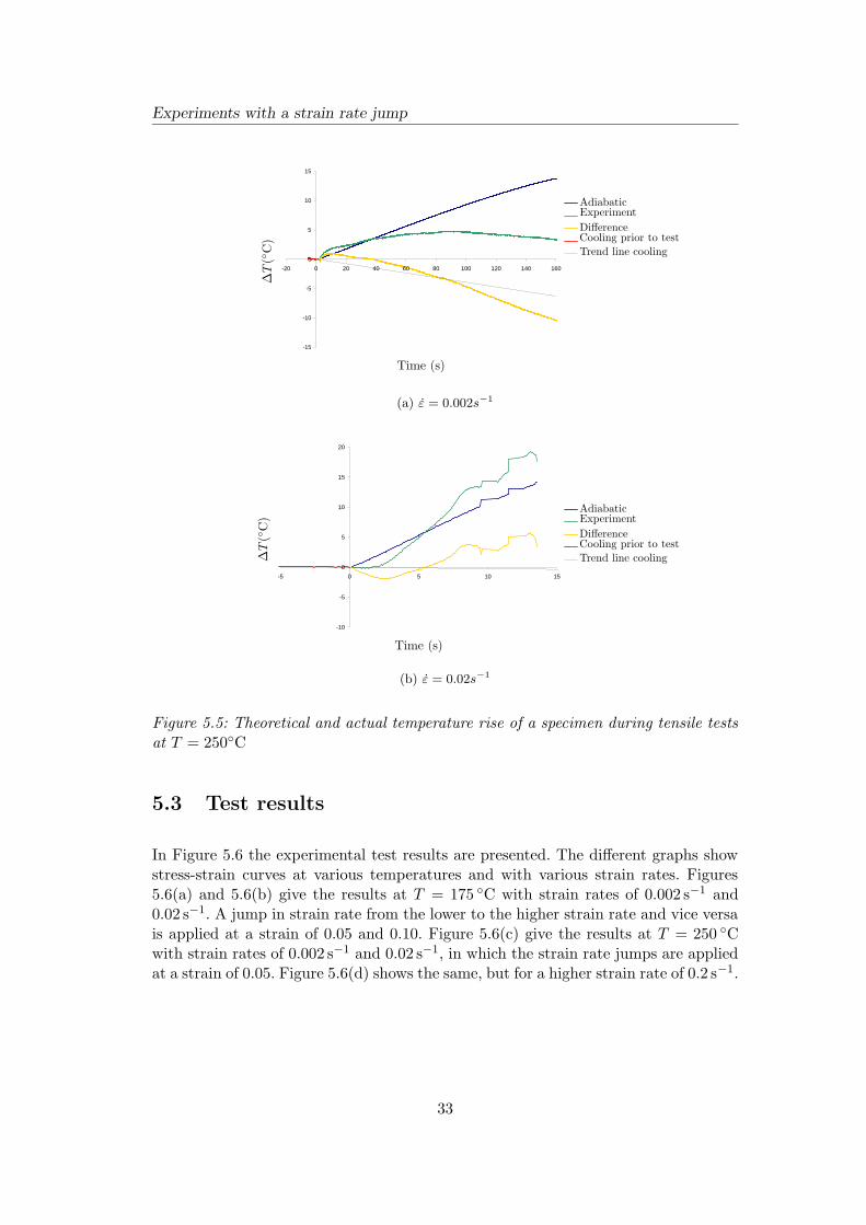
During testing a tensile specimen can undergo an appreciable temperature rise. Thisis because most of the mechanical energy used to deform the specimen is convertedinto heat. The temperature rise of the specimen depends on the energy inserted by thetest machine and on the amount of heat lost to the environment. If the test is rapidenough little heat is lost and the temperature rise can be surprisingly high. A hightemperature rise in the specimen could have a significant influence on the measuredproperties, so it is important to know how much the temperature rises during theconducted tensile tests [9].
A first approximation of the temperature rise is available by assuming that the energyconversion process is adiabatic. In that case all the energy used for producing plasticdeformation appears as heat. Assuming no heat is emitted to the environment, thetemperature rise ∆T can be calculated with:
∆T =u
cρ(5.2)
With u the energy per volume, c the specific heat and ρ the density. For aluminiummagnesium alloys c = 960 J/kgK and ρ = 2650 kg/m3 [17]. The energy per volume uis equal to the surface beneath the engineering stress-strain curve:
u =
∫
Sde (5.3)
In Figure 5.5 the (calculated) adiabatical and experimental temperature rise dur-ing two tensile tests and the difference between these two temperatures are given.Furthermore the rate of cooling was measured prior to the tensile test and a trendline for this cooling was extrapolated. In Figure 5.5(a) it can be seen that for lowstrain rates the difference between the theoretical and actual temperature rise is al-most equal to the cooling trend line. The total temperature rise stays below 5 C.For tests at higher strain rates, see Figure 5.5(b), there is not enough time for thespecimen to cool down. Therefore the temperature rise of the specimen during testingis almost 20 C. However, the ultimate tensile strength for tests at 250 C is reachedat a strain of 0.1. The temperature rise at this point is only 5 C so the temperaturerise is not expected to have a large influence for the stress-strain curves up to uniformstrain.
32
Experiments with a strain rate jump
-15
-10
-5
0
5
10
15
-20 0 20 40 60 80 100 120 140 160
PSfrag replacements
Time (s)
∆T(C)
AdiabaticExperiment
DifferenceCooling prior to test
Trend line cooling
(a) ε = 0.002s−1
-10
-5
0
5
10
15
20
-5 0 5 10 15
PSfrag replacements
Time (s)
∆T(C)
AdiabaticExperiment
DifferenceCooling prior to test
Trend line cooling
(b) ε = 0.02s−1
Figure 5.5: Theoretical and actual temperature rise of a specimen during tensile testsat T = 250C
5.3 Test results
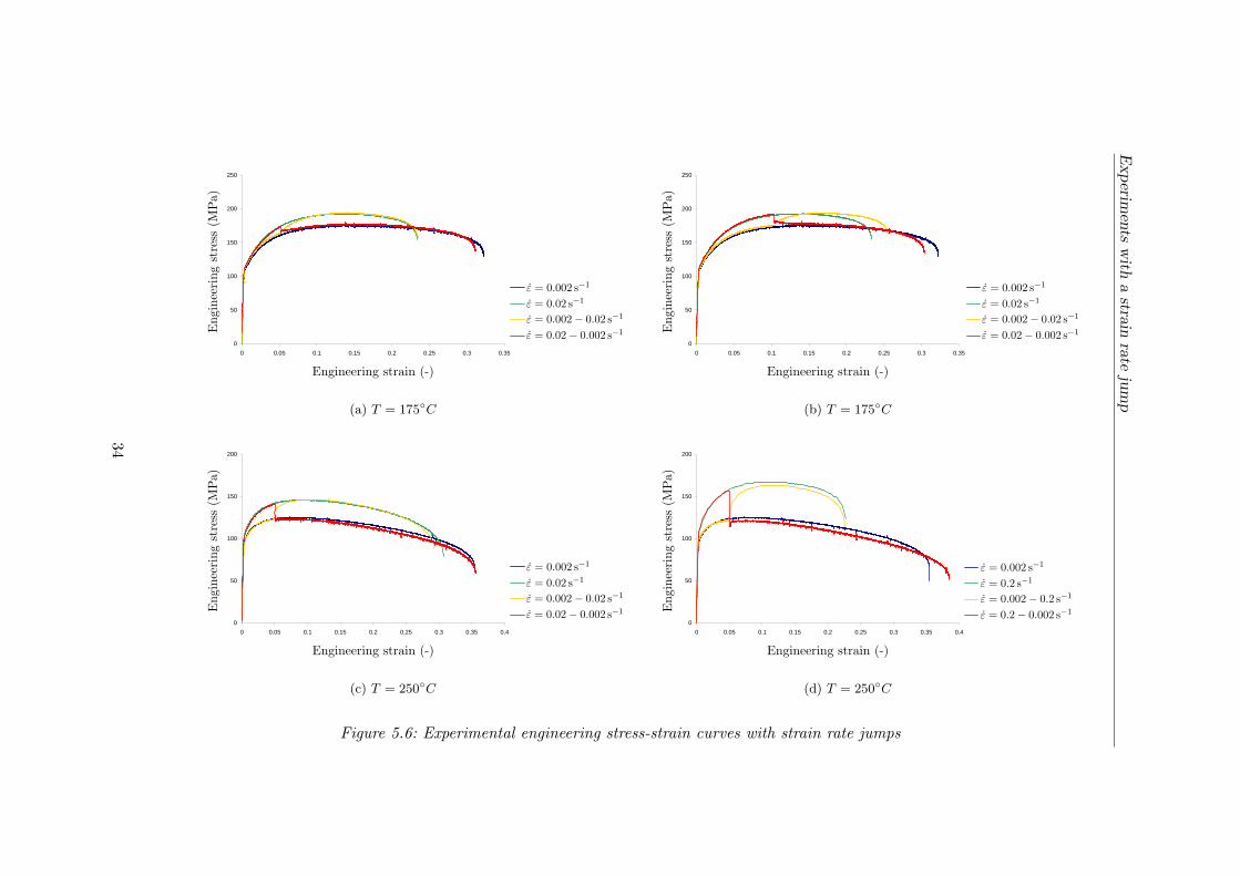
In Figure 5.6 the experimental test results are presented. The different graphs showstress-strain curves at various temperatures and with various strain rates. Figures5.6(a) and 5.6(b) give the results at T = 175 C with strain rates of 0.002 s−1 and0.02 s−1. A jump in strain rate from the lower to the higher strain rate and vice versais applied at a strain of 0.05 and 0.10. Figure 5.6(c) give the results at T = 250 Cwith strain rates of 0.002 s−1 and 0.02 s−1, in which the strain rate jumps are appliedat a strain of 0.05. Figure 5.6(d) shows the same, but for a higher strain rate of 0.2 s−1.
33
Experim
ents
with
astra
inra
teju
mp
0
50
100
150
200
250
0 0.05 0.1 0.15 0.2 0.25 0.3 0.35
PSfrag replacements
Engineering strain (-)
Engineeringstress
(MPa)
ε = 0.002 s−1
ε = 0.02 s−1
ε = 0.002− 0.02 s−1
ε = 0.02− 0.002 s−1
(a) T = 175C
0
50
100
150
200
250
0 0.05 0.1 0.15 0.2 0.25 0.3 0.35
PSfrag replacements
Engineering strain (-)
Engineeringstress
(MPa)
ε = 0.002 s−1
ε = 0.02 s−1
ε = 0.002− 0.02 s−1
ε = 0.02− 0.002 s−1
(b) T = 175C
0
50
100
150
200
0 0.05 0.1 0.15 0.2 0.25 0.3 0.35 0.4
PSfrag replacements
Engineering strain (-)
Engineeringstress
(MPa)
ε = 0.002 s−1
ε = 0.02 s−1
ε = 0.002− 0.02 s−1
ε = 0.02− 0.002 s−1
(c) T = 250C
0
50
100
150
200
0 0.05 0.1 0.15 0.2 0.25 0.3 0.35 0.4
PSfrag replacements
Engineering strain (-)
Engineeringstress
(MPa)
ε = 0.002 s−1
ε = 0.2 s−1
ε = 0.002− 0.2 s−1
ε = 0.2− 0.002 s−1
(d) T = 250C
Figure 5.6: Experimental engineering stress-strain curves with strain rate jumps
34
Experiments with a strain rate jump
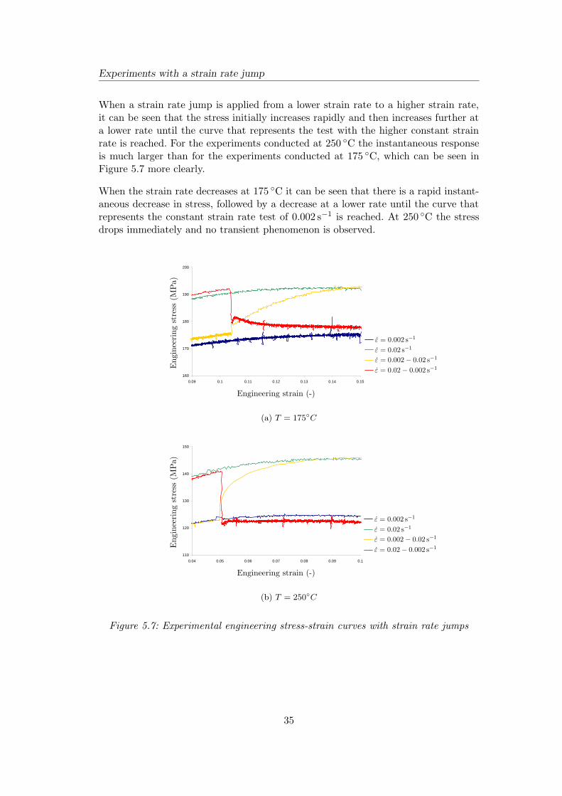
When a strain rate jump is applied from a lower strain rate to a higher strain rate,it can be seen that the stress initially increases rapidly and then increases further ata lower rate until the curve that represents the test with the higher constant strainrate is reached. For the experiments conducted at 250 C the instantaneous responseis much larger than for the experiments conducted at 175 C, which can be seen inFigure 5.7 more clearly.
When the strain rate decreases at 175 C it can be seen that there is a rapid instant-aneous decrease in stress, followed by a decrease at a lower rate until the curve thatrepresents the constant strain rate test of 0.002 s−1 is reached. At 250 C the stressdrops immediately and no transient phenomenon is observed.
160
170
180
190
200
0.09 0.1 0.11 0.12 0.13 0.14 0.15
PSfrag replacements
Engineering strain (-)
Engineeringstress
(MPa)
ε = 0.002 s−1
ε = 0.02 s−1
ε = 0.002− 0.02 s−1
ε = 0.02− 0.002 s−1
(a) T = 175C
110
120
130
140
150
0.04 0.05 0.06 0.07 0.08 0.09 0.1
PSfrag replacements
Engineering strain (-)
Engineeringstress
(MPa)
ε = 0.002 s−1
ε = 0.02 s−1
ε = 0.002− 0.02 s−1
ε = 0.02− 0.002 s−1
(b) T = 250C
Figure 5.7: Experimental engineering stress-strain curves with strain rate jumps
35
Experiments with a strain rate jump
5.4 Comparing experiments with the material models
Section 3.2.4 described how both the extended Nadai and Bergstrom models predictedthe material behaviour in case of a strain rate jump. In Figure 3.6 it could be seenthat the extended Nadai model predicts an immediate response of the material, whilethe Bergstrom model predicts a slow approach of the constant strain rate curve.
As illustrated in Figure 5.6, the material behaviour is somewhere in the middle: thereis an immediate response as predicted by the extended Nadai model, followed bya slower response as predicted by the Bergstrom model. For higher temperatures(250 C) there is a larger immediate response, which means that the extended Nadaimodel predicts this behaviour better. This outcome is surprising as the extendedNadai model is a phenomenological model and is based on responses of the model toa constant strain rate and temperature. The Bergstrom model, however, is physicallybased, and it was expected that it would therefore predict the material behaviourduring a strain rate jump better. However, this is not the case, so it is suggested thatfurther research is conducted during which this material model is investigated furtherto see if by including more information in the model, e.g. the observed temperaturedependence of the response to a jump in the strain rate, it can be improved.
36
Chapter 6
Conclusions and
recommendations
In this chapter the conclusions from the current research and recommendations forfuture research are presented.
6.1 Conclusions
To model the material behaviour of aluminium-magnesium alloys at elevated temper-atures a phenomenological model (the extended Nadai model) and a physically basedmodel (the Bergstrom model) were presented and used in this thesis. The parametersof these models were determined by fitting the models to stress-strain curves obtainedfrom constant strain rate tests performed at TNO Eindhoven for various temperat-ures and strain rates. For constant strain rate both models predicted the stress-straincurves reasonably accurate. The Bergstrom model describes the material behaviourslightly better than the extended Nadai model.
When using the Bergstrom model in a finite element simulation, it was seen that themodel is able to describe the material behaviour of aluminium in uniaxial deforma-tion at elevated temperatures and constant strain rates successfully. The stress-straincurves were predicted accurately up to the ultimate tensile strength. After neckingthe numerical simulations have approximately the same softening slope as the exper-imental results, although in the numerical analysis localisation starts earlier.
When a strain rate jump is applied, the two material models predict completelydifferent responses. The extended Nadai model predicts an instantaneous stress jump,whereas the Bergstrom model predicts a gradual change in stress until the curve thatcorresponds to the new strain rate is reached. Experiments that have been performedat the University of Twente showed that the actual material behaviour is somewherein the middle: there is an immediate response as predicted by the extended Nadaimodel, followed by a slower response as predicted by the Bergstrom model. For higher
37
Conclusions and recommendations
temperatures (250 C) there is a larger immediate response, which means that theextended Nadai model predicts this behaviour better.
6.2 Recommendations
Strain rates and temperatures are usually not constant during forming processes atelevated temperatures. For numerical simulations a model that describes the materialbehaviour in case of a strain rate jump more accurately should be developed. It istherefore recommended that the Bergstrom model is investigated further to see if itcan be improved by including more information into the model, e.g. the observedtemperature dependence of the response to a jump in the strain rate.
Since the material behaviour changes significantly between 175 C and 250 C it isrecommended that more experiments with a strain rate jump are performed at inter-mediate temperatures. Next to that, it could also be useful to investigate the materialbehaviour at somewhat lower temperatures to see if the Bergstrom model is more ac-curate at lower temperatures. For these experiments the furnace should be covered,to decrease the temperature gradient over the specimen, which makes the test resultsmore easy to compare with other experiments. It is also recommended that whenfurther tests are performed a more sophisticated feedback system for the furnace isdeveloped. As a result the heating of the specimens will be easier to regulate.
A final recommendation that can be made is to update the software used to control thetensile testing machine. When this is implemented it is possible to not only performexperiments with a single or even multiple strain rate jumps, but also to performtensile tests with a gradual change in strain rate. It would be interesting to knowhow the material behaves when deformed in this way since this gives an even betterapproximation of the deep drawing process.
38
Bibliography
[1] Bergstrom, Y. Dislocation model for the stress-strain behaviour of polycrys-talline α-Fe with special emphasis on the variation of the densities of mobile andimmobile dislocations. Mater. Sci. Eng. 5 (1969), 193–200.
[2] Bergstrom, Y. The plastic deformation of metals - a dislocation model andits applicability. Reviews on Powder Metalurgy and Physical Ceramics 2 (1983),105–115.
[3] Bolt, P. J., Lamboo, N. A. P. M., and Rozier, P. J. C. M. Feasibilityof warm drawing of aluminium products. In Sheet Metal 1999 (Erlangen, 1999),M. Geiger, H. J. J. Kals, B. Shirvani, and U. P. Singh, Eds., pp. 575–580.
[4] Bolt, P. J., Werkhoven, R. J., and Van den Boogaard, A. H. Effectof elevated temperatures on the drawability of aluminium sheet components. InProceedings 4th Esaform Conference (Liege, 2001).
[5] Boyer, H. E., Ed. Atlas of stress-strain curves. ASM International, 1987. ISBN0-87170-240-1.
[6] Callister, W. D. Materials science and engineering. John Wiley and Sons,Inc., 1985.
[7] Davis, J. R., Ed. ASM Speciality Handbook, Aluminum and aluminum alloys.ASM International, 1993. ISBN 0-87170-496-X.
[8] Estrin, Y. Dislocation-density–related constitutive modeling. In Unified Con-stitutive Laws of Plastic Deformation, A. S. Krausz and K. Krausz, Eds. Aca-demic Press, San Diego, 1996, pp. 69–104.
[9] Han, P., Ed. Tensile testing. ASM International, 1992. ISBN 0-87170-440-4.
[10] Hertzberg, R. W. Deformation and fracture mechanics of engineering mech-anics. John Wiley and Sons, Inc., 1989.
[11] Krabiell, A., and Dahl, W. Zum Einfluss von Temperatur undDehngeschwindigkeit auf die Streckgrenze von Baustahlen unterschiedlicher Fest-igkeit. Archiv fur das Eisenhuttenwesen 52 (1981), 429–436.
[12] Kuhn, H., and Medlin, D., Eds. ASM Handbook, Volume 8: Mechanical testingand evaluation. ASM International, 2000. ISBN 0-87170-389-0.
39

BIBLIOGRAPHY
[13] Miller, W. S., Zhuang, L., Bottema, J., Wittebrood, A. J., de Smet,P., Haszler, A., and Vieregge, A. Recent developments in aluminium alloysfor the automotive industry. Materials Science and Engineering A 280 (2000),37–49.
[14] Nelder, J. A., and Mead, R. A simplex method for function minimization.Computer Journal 7 (1965), 308–313.
[15] Olivier, J. G. J., Brandes, L. J., Peters, J. A. H. W., and Coenen,P. Greenhouse gas emissions in the Netherlands 1999-2000. RIVM, Bilthoven,2002.
[16] Rietman, A. D. Numerical Analysis of Inhomogeneous Deformation in PlaneStrain Compression. PhD thesis, University of Twente, 1999.
[17] Stiomak/tht. Materiaalkeuze in de werktuigbouwkunde. Stam TechnischeBoeken, Culemborg, 1978.
[18] van den Boogaard, A. H. Thermally enhanced forming of aluminium sheet.PhD thesis, University of Twente, 2002.
[19] van den Boogaard, A. H., Bolt, P., and Werkhoven, R. J. Aluminumsheet forming at elevated temperatures. In Simulation of Materials Processing:Theory, Methods and Applications (Lisse, 2001), K.-I. Mori, Ed., A.A. Balkema,pp. 819–824.
[20] van den Boogaard, A. H., Werkhoven, R. J., and Bolt, P. Modellingof AlMg sheet forming at elevated temperatures. In International Journal ofForming Processes (2001), vol. 4, pp. 361–375.
[21] van Liempt, P. Workhardening and substructural geometry of metals. J. Mater.Process. Technol. 45 (1994), 459–464.
40
Acknowledgements
This thesis is written to conclude my studies of Mechanical Engineering at the Uni-versity of Twente and is the result of an extended research period at the sectionMechanics of Forming Processes.
I would like to thank everyone who has supported me and made a contribution tothis graduation project. Especially I would like to thank the following people:
• My supervisor, Ton van den Boogaard, for his support, suggestions and helpfuldiscussions.
• Erik van der Ven and Joop Brinkman for their help with the experimental partof this project and the many interesting discussions.
• Joop Brinkman again for taking care of the design and manufacturing of theclamps and test specimens and proof-reading this report.
• Jaco van Leeuwen and Peter de Maat from TNO Eindhoven who performed theuniaxial tensile tests for a constant strain rate.
• My family and friends because of their continuous support and patience.
• Finally I would like to thank the fellow students with whom I cooperated duringmost of my studies in our project team and the students and members of thesection Mechanics of Forming Processes for giving me a pleasant time duringmy studies.
41