delay learning and polychronization for reservoir...

Delay Learning and Polychronization for

Reservoir Computing

Helene Paugam-Moisy a,∗ Regis Martinez a and Samy Bengio b

aLIRIS, UMR CNRS 5205, Universite Lyon 2, France

bGoogle, 1600 Amphitheatre Pkwy, B1350-138B, Mountain View, CA 94043, USA

Abstract

We propose a multi-timescale learning rule for spiking neuron networks, in the lineof the recently emerging field of reservoir computing. The reservoir is a networkmodel of spiking neurons, with random topology and driven by STDP (Spike-Time-Dependent Plasticity), a temporal Hebbian unsupervised learning mode, biologicallyobserved. The model is further driven by a supervised learning algorithm, basedon a margin criterion, that affects the synaptic delays linking the network to thereadout neurons, with classification as a goal task. The network processing andthe resulting performance can be explained by the concept of polychronization,proposed by Izhikevich (2006, Neural Computation, 18:2), on physiological grounds.The model emphasizes that polychronization can be used as a tool for exploitingthe computational power of synaptic delays and for monitoring the topology andactivity of a spiking neuron network.

Key words: Reservoir Computing, Spiking Neuron Network, Synaptic Plasticity,STDP, Polychronization, Programmable Delay, Margin Criterion, Classification

∗ LIRIS, UMR CNRS 5205, Bat. C, Universite Lumiere Lyon 2, 5 avenue PierreMendes France, F-69676 Bron cedex, France

Email addresses: [email protected] (Helene Paugam-Moisy),[email protected] (Regis Martinez), [email protected] (SamyBengio).

URLs: http://liris.cnrs.fr/membres?idn=hpaugam (HelenePaugam-Moisy), http://liris.cnrs.fr/membres?idn=rmartine (RegisMartinez), http://bengio.abracadoudou.com (Samy Bengio).

Preprint submitted to Elsevier 26 December 2007

1 Introduction

1.1 Reservoir Computing

Reservoir Computing (RC) recently appeared [38,17] as a generic name for de-signing a new research stream including mainly Echo State Networks (ESNs)[15,16], Liquid State Machines (LSMs) [25], and a few other models like Back-propagation Decorrelation (BPDC) [42]. Although they have been discoveredindependently, the algorithms share common features and carry many highlychallenging ideas toward a new computational paradigm of neural networks.The central specification is a large, distributed, nonlinear recurrent network,the so-called “reservoir”, with trainable output connections, devoted to read-ing out the internal states induced in the reservoir by input patterns. Usually,the internal connections are sparse and their weights are kept fixed. Accordingto the model, the reservoir can be composed of different types of neurons, e.g.linear units, sigmoid neurons, threshold gates or spiking neurons (e.g. LIF 1 ),as far as the internal network behaves like a non linear dynamical system. Inmost models, simple learning rules, such as linear regression or recursive leastmean squares are applied to readout neurons only. In the editorial of the spe-cial issue of Neural Networks [17], several directions for further research havebeen pointed out, among them is “the development of practical methods tooptimize a reservoir toward the task at hand”. In the same article, RC is pre-sented as belonging to the “family of versatile basic computational metaphorswith a clear biological footing”. The model we developed [34] is clearly basedon similar principles: A network of spiking neurons, sparsely connected, with-out pre-imposed topology, and output neurons, with adaptable connections.

As stated in [38], the concept that is considered to be a main advantage of RCis to use a fixed randomly connected network as reservoir, without trainingburden. Recent work also propose to add an unsupervised reservoir adaptationthrough various forms of synaptic plasticity such as Spike-Time-DependentPlasticity [31] or Intrinsic Plasticity [47,50] (see [21] for a comparative study).However, many articles point out the difficulty to get a suitable reservoirw.r.t. a given task. According to the cognitive metaphor, the brain may beviewed as a huge reservoir able to process a wide variety of different tasks,but synaptic connections are not kept fixed in the brain: Very fast adaptationprocesses compete with long term memory mechanisms [18]. Although themystery of memory and cognitive processing is far from being solved, recentadvances in neuroscience [2,28,41] help to get new inspiration for conceivingcomputational models. Our learning rule for readout neurons is justified by

1 LIF = Leaky Integrate and Fire

2

the appealing notion of polychronization [14] from which Izhikevich derivesan explanation for a theoretically “infinite” capacity of memorizing in thebrain. We based our method to adapt the reservoir to the current task on animplementation of synaptic plasticity inside a Spiking Neuron Network (SNN)and on the exploitation of the polychronization concept.

1.2 Spiking Neuron Networks

A common thought that interactions between neurons are governed by theirmean firing rates has been the basis of most traditional artificial neural net-work models. Since the end of the 90’s, there is a growing evidence, both inneuroscience and computer science, that precise timing of spike firing is a cen-tral feature in cognitive processing. SNNs derive their strength and interestfrom an accurate modeling of synaptic interactions between neurons, takinginto account the time of spike firing. Many biological arguments, as well astheoretical results (e.g. [22,37,40]) converge to establish that SNNs are po-tentially more powerful than traditional artificial neural networks. However,discovering efficient learning rules adapted to SNNs is still a hot topic. Forthe last ten years, solutions were proposed for emulating classic learning rulesin SNNs [24,30,4], by means of drastic simplifications that often resulted inlosing precious features of firing time based computing. As an alternative,various researchers have proposed different ways to exploit recent advancesin neuroscience about synaptic plasticity [1], especially IP 2 [10,9] or STDP 3

[28,19], that is usually presented as the Hebb rule, revisited in the context oftemporal coding. A current trend is to propose computational justificationsfor plasticity-based learning rules, in terms of entropy minimization [5] as wellas log-likelihood [35] or mutual information maximization [8,46,7]. However,since STDP is a local unsupervised rule for adapting the weights of connec-tions, such a synaptic plasticity is not efficient enough for controlling the be-havior of an SNN in the context of a given task. Hence we propose to coupleSTDP with another learning rule, acting at a different time scale.

1.3 Multi-timescale Learning

We propose to name “multi-timescale learning” a learning rule combining atleast two adaptation algorithms, at different time scales. For instance, synapticplasticity, modifying the weights locally, in the millisecond time range, can becoupled with a slower overall adaptation rule, such as reinforcement learning

2 IP = Intrinsic Plasticity3 STDP = Spike-Time-Dependent Plasticity

3

driven by an evolutionary algorithm, like in [29], or a supervised learningalgorithm, for classification purpose, as developed in the present article.

The multi-timescale learning rule we propose is motivated by two main ideas:

• Delay adaptation: Several complexity analyzes of SNNs have proved theinterest of programmable delays for computational power [22,37] and learn-ability [26,27,23]. Although axonal transmission delays do not vary contin-ually in the brain, a wide range of delay values have been observed.

• Polychronization: In [14] Izhikevich pointed out the activation of poly-chronous groups, based on the variability of transmission delays inside anSTDP-driven set of neurons (see Section 5 for details), and proposed thatthe emergence of several polychronous groups, with persistent activation,could represent a stimulation pattern.

Our multi-timescale learning rule for reservoir computing is comprised ofSTDP, modifying the weights inside the reservoir, and a supervised adap-tation of axonal transmission delays toward readout neurons coding, via theirtimes of spike firing, for different classes. Without loss of generality, the modelis mainly presented in the two-class version. The basic idea is to adapt theoutput delays in order to enhance the influence of the polychronous groupsactivated by a given pattern toward the target output neuron, and to decreasethe influence toward the non-target neuron. A margin criterion is applied, via astochastic iterative learning process, for strengthening the separation betweenthe spike-timing of the readout (output) neurons. This idea fits in the similar-ity that has been recently proposed [38,17] between RC and SVM 4 , where thereservoir is compared to the high-dimensional feature space resulting from akernel transformation. In our algorithm, like in the machine learning literature,the application of a margin criterion is justified by the fact that maximizinga margin between the positive and the negative class yields better expectedgeneralization performance [48].

We point out that polychronization can be considered as a tool for adaptingsynaptic delays properly, thus exploiting their computational power, and forobserving the network topology and activity.

The outline of the papers goes as follows: Section 2 describes the model ofspiking neuron network (SNN) for reservoir computing (RC); Section 3 definesthe multi-scale learning mechanism; experiments on classification tasks arepresented in Section 4; Section 5 explains the notion of polychronization andSection 6 studies the internal dynamics of the reservoir.

4 SVM = Support Vector Machine

4

2 Network Architecture

The reservoir is a set of M neurons (internal network), interfaced with a layerof K input cells and C readout cells, one for each class (Figure 1). The networkis fed by input vectors of real numbers, represented by spikes in temporalcoding: The higher the value, the earlier the spike fires toward the reservoir.For clarity in experiments, successive inputs are presented in large temporalintervals, without overlapping input spike firing from a pattern to the next.The index of the output cell firing first in this temporal interval provides theclass number as an answer of the network to the input pattern.

.

.

.cells

K input

class 1

class 2

2 output cells

internal connections

output connections,

input connections

with adaptable delays

M internal cells

Fig. 1. Architecture of the spiking neuron network. The reservoir is the internalnetwork (the colored square) and green (light grey) links represent the interfacewith environment. The network is presented for C = 2 classes.

Each cell is a spiking neuron (Section 2.1). Each synaptic connection, fromneuron Ni to neuron Nj, is defined by two parameters: A weight wij and an ax-onal transmission delay dij. The reservoir is composed of 80% excitatory neu-rons and 20% inhibitory neurons, in accordance with the ratio observed in themammalian cortex [6]. The internal connectivity is random and sparse, withprobability Prsv for a connection to link Ni to Nj, for all (i, j) ∈ {1, ...,M}2.For pattern stimulation, the input cells are connected to the internal cells withprobability Pin. The connection parameters are tuned so that the input cellsforward spikes toward internal cells according to the temporal pattern definedby the input stimulus (see Section 2.2). For class detection, the output neuronsare fully connected to each internal cell (Pout = 1).

2.1 Neuron Model

The neuron model is an SRM0 (zero’th order “Spike Response Model”), asdefined by Gerstner [12], where the state of a neuron Nj is dependent on

its last spike time t(f)j only. The next firing time of Nj is governed by its

membrane potential uj(t), in millivolts, and its threshold θj(t). Both variablesdepend on the last firing times of the neurons Ni belonging to the set Γj ofneurons pre-synaptic to Nj:

5

uj(t) = η(t − t(f)j )

︸︷︷︸

threshold kernel

+∑

i∈Γj

wij ǫ(t − t(f)i − dij)

︸︷︷︸

potential kernel

+ urest (1)

firing condition for Nj uj(t) ≥ ϑ with u′

j(t) > 0 =⇒ t(f+1)j = t (2)

The potential kernel is modelled by a Dirac increase in 0, followed by an exponentialdecrease, from value umax in 0+ toward 0, with a time constant τm, in milliseconds:

ǫ(s) = umaxH(s)e(−

sτm

)

(3)

where H is the Heaviside function. In Equation (2) the value wij is a positive factorfor excitatory weights and a negative one for inhibitory weights.

The firing threshold ϑ is set to a fixed negative value (e.g. ϑ = −50 mV ) andthe threshold kernel simulates an absolute refractory period τabs, when the neuroncannot fire again, followed by a reset to the resting potential urest, lower than ϑ (e.g.urest = −65 mV ). The relative refractory period is not simulated in our model. Thesimulation is computed in discrete time with 1 ms time steps. Time steps 0.1 mslong have been tested also (Section 4.2). The variables of neuron Nj are updatedat each new incoming spike (event-driven programming), which is sufficient forcomputational purpose.

2.2 Weights and Delays

Synaptic plasticity (see Section 3.1) is applied to the weights of internal cells only.Starting from initial values w such that ‖w‖ = 0.5, internal weights vary, underSTDP, in the range [0, 1] (excitatory) or [−1, 0] (inhibitory). The weights of con-nections from input layer to internal network are kept fixed, all of them excitatory,with a value win strong enough to induce immediate spike firing inside the reser-voir (e.g. win = 3 in experiments, see Section 4). The connections from internalnetwork to output neurons are excitatory and the output weights are fixed to theintermediate value wout = 0.5. In principle, STDP can be applied also to the outputweights (optional in our program) but no improvement has been observed. Hence,for saving computational cost, the readout learning rule has been further restrictedto an adaptation of the synaptic delays (Section 3.2).

Neuroscience experiments [44,45] give evidence to the variability of transmissiondelay values, from 0.1ms to 44ms. In the present model, the delays dij take integervalues, randomly chosen in {dmin, . . . , dmax}, rounded to the nearest millisecond,both in the internal network and toward readout neurons. The delays from inputlayer to internal network have a zero value, for an immediate transmission of inputinformation.

6

A synaptic plasticity rule could be applied to delay learning, as well as to weightlearning, but the biological plausibility of such a plasticity is not yet so clear inneuroscience [39]. Moreover our purpose is to exploit this stage of the learning rulefor making easier the adaptation of the reservoir to a given task. Hence we do notapply synaptic plasticity to delays, but we switch to machine learning in designing asupervised mechanism, based on a margin criterion, for adapting the output delaysto the reservoir computation in order to extract the relevant information.

3 Learning Mechanisms

In the model, the multi-timescale learning rule is based on two concurrent mecha-nisms: A local unsupervised learning of weights by STDP, operating in the millisec-ond range, at each new incoming spike time tpre or outgoing spike time tpost, anda supervised learning of output delays, operating in the range of 100 ms, at eachpattern presentation.

3.1 Synaptic Plasticity

The weight wij of a synapse from neuron Ni to neuron Nj is adapted by STDP, aform of synaptic plasticity based on the respective order of pre- and post-synapticfiring times. For excitatory synapses, if a causal order (pre- just before post-) isrespected, then the strength of the connection is increased. Conversely the weightis decreased if the pre-synaptic spike arrives at neuron Nj just after a post-synapticfiring, and has probably no effect, due to the refractory period of Nj . For inhibitorysynapses, only a temporal proximity leads to a weight increase, without causal effect.Temporal windows, inspired from neurophysiological experiments by Bi & Poo [3],help to calculate the weight modification ∆W as a function of the time difference

∆t = tpost − tpre = t(f)j − (t

(f)i + dij) as can be computed at the level of neuron Nj .

1.0

POTENTIATION

DEPRESSION −0.5

t

W

10ms 20ms

100ms

1.0

t

W

20ms−20ms

−0.25

DEPRESSION DEPRESSION

POTENTIATION

+infini−infini

Fig. 2. Asymmetrical STDP temporal window for excitatory (left) and symmetricalSTDP temporal window for inhibitory (right) synapse adaptation (from [29]).

For updating excitatory synapses as well as inhibitory synapses, a similar princi-ple is applied, and only the temporal windows differ (see Figure 2). For updatingexcitatory synapses, we adopt the model of Nowotny [32] with an asymmetrical

7

shape of temporal window. For inhibitory synapses, weight updating is based on acorrelation of spikes, without influence of the temporal order, as proposed in [51].

Following [36], in order to avoid a saturation of the weights to the extremal valueswmin = 0 and wmax = 1 (excitatory) or wmax = −1 (inhibitory), we apply amultiplicative learning rule, as stated in Equation (4), where α is a positive learningrate. In our experiments: α = αexc = αinh = 0.1. For excitatory synapses the signof ∆W is the sign of ∆t. For inhibitory synapses ∆W > 0 iff | ∆t |< 20.

if ∆W ≤ 0 depreciate the weight: wij ← wij + α ∗ (wij − wmin) ∗ ∆W

if ∆W ≥ 0 potentiate the weight: wij ← wij + α ∗ (wmax − wij) ∗ ∆W (4)

STDP is usually applied with an additive rule for weight modification and manyauthors observe a resulting bimodal distribution of weights, with an effect of satura-tion toward the extremal values. In [21] Lazar et al. propose to couple IP (IntrinsicPlasticity) with STDP and show that the effect of saturation is reduced. We ob-tain a similar result with a multiplicative rule (see Section 4.1.3), but at a lowercomputational cost.

3.2 Delay Adaptation Algorithm

The refractory period of the readout neurons has been set to a value τ outabs , large

enough to trigger at most one output firing for each neuron, inside a temporalwindow of T ms dedicated to an input pattern presentation.

The goal of the supervised learning mechanism is to modify the delays from activeinternal neurons to readout neurons in such a way that the output neuron corre-sponding to the target class fires before the one corresponding to the non-targetclass. Moreover, we intend to maximize the margin between the positive and thenegative class. More formally, the aim is to minimize the following criterion:

C =∑

p∈class1

|t1(p) − t2(p) + µ|+ +∑

p∈class2

|t2(p) − t1(p) + µ|+ (5)

where ti(p) represents the firing time of readout neuron Outi after the presentationof input pattern p, µ represents the minimum delay margin we want to enforcebetween the two firing times, and |z|+ = max(0, z). The margin constant µ is ahyper-parameter of the model and can be tuned according to the task at hand.Convenient values are a few milliseconds, e.g. µ = 5 or µ = 8 in experiments(Section 4).

In order to minimize the criterion (5), we adopt a stochastic training approach,iterating a delay adaptation loop, as described in Algorithm 1. We define a triggering

8

connection as a connection that carries an incoming spike responsible for a post-synaptic spike firing at the impact time. Due to the integer values of delays and thediscrete time steps for computation, it may occur that several triggering connectionsaccumulate their activities at a given iteration. In such a case, we choose only oneamong these candidate connections for delay adaptation.

Algorithm 1 (two-class):

repeat

for each example X = (p, class) of the database

{ present the input pattern p;define the target output neuron according to class;if ( the target output neuron fires less than µ ms before

the non-target output neuron, or fires after it )

then

{ select one triggering connection of the target output

neuron and decrement its delay (−1 ms), except if

dmin is reached already;

select one triggering connection of the non-target

output neuron and increment its delay (+1 ms), except

if dmax is reached already;

}}

until a given maximum learning time is over.

As an illustration, let us consider an input pattern belonging to class 2. Hence wewant output neuron Out2 to fire at least µ milliseconds before output neuron Out1.Figure 3 shows the variation through time of the membrane potential of the tworeadout neurons. Note that, without loss of generality, the curves of exponentialdecrease have been simplified into straight oblique lines, to represent variations ofu(t). The effect of one iteration of delay learning on the respective firing times isdepicted from the left graphic (step k) to the right one (step k + 1). At step k, thedifference between firing times of the two output neurons is lower than µ, whereasat step k + 1 the pattern is well classified, with respect to the margin.

Although the context is not always as auspicious as in Figure 3, even so, at eachiteration where a delay adaptation occurs, the probability of an error in the nextanswer to a similar input has decreased. Actually, under the hypothesis that therecent history of the membrane potential is similar between the current and thenext presentation of a pattern p (verified condition in Figure 3), the increment ofthe delay of the non-target neuron leads to a later firing of Out1 with probability1. Under similar conditions, if the triggering connection of the target neuron isalone, the decrement of its delay causes a 1 ms earlier spike, thus incoming inaddition to a higher value of the membrane potential as far as the time constant τm

generates an exponential decrease less than 0.5 (equal to the contribution of wout)in a 1 ms time range, hence the readout neuron Out1 fires earlier, with probability1. The only hazardous situation occurs in case of multiple triggering connections,

9

u(t)mV

t [ms]

u(t)mV

t [ms]

u(t)mV

t [ms]

u(t)mV

Out 2Out 1 t [ms]

µ

t [ms]

Out 1Out 2

t [ms]

potential of Out 1 potential of Out 1

potential of Out 2

membrane potential of Out 2

step k of delay learning iterations step k+1 of delay learning iterations

µ

Fig. 3. An example illustrating the effect of one iteration of the delay learningalgorithm on the firing times of the two readout neurons.

where configurations exist for later firing of Out1, but with a probability close to 0,since the sparse connectivity of the reservoir induces a low internal overall spikingactivity (usually close to 0.1 in experimental measurements). Finally, the hypothesisof membrane potential history conservation is not highly constraining, since theaction of STDP has the effect of reinforcing the weights of the connections, in thereservoir, that are responsible for relevant information transmission. Therefore, asthe learning process goes through time, spike-timing patterns become very stable,as could be observed experimentally (see raster plots in Section 4.1.1).

3.3 Extension to Multi-Class Discrimination

The multi-timescale learning rule can be extended to multi-class discrimination. Thenetwork architecture is similar (Figure 1), except that the output layer is composedof C readout neurons, one for each of the C classes. The response of the network toan input pattern p is the index of the first firing output neuron. Whereas synapticplasticity is unchanged, the delay adaptation algorithm has to be modified andseveral options arise, especially concerning the action on one or several non-targetneurons. We propose to apply Algorithm 2.

A variant could be to increment the delays of all the first firing non-target outputneurons. Since the performance improvement is not clear, in experiments the ad-vantage has been given to Algorithm 2, i.e. with at most one delay adaptation ateach iteration, in order to save computational cost.

10

Algorithm 2 (multi-class):

repeat

for each example X = (p, class) of the database

{ present the input pattern p;define the target output neuron according to class;if ( the target output neuron fires less than µ ms before

the second firing time among non-target output neurons,

or fires later than one or several non-target neurons )

then

{ randomly select one triggering connection of the target

output neuron and decrement its delay (−1 ms), except

if dmin is reached already;

randomly select one neuron among all the non-target

readouts that fired in first;

for this neuron, randomly select one triggering

connection and increment its delay (+1 ms), except if

dmin is reached already;

}}

until a given maximum learning time is over.

4 Experiments

A first set of experiments has been performed on a pair of very simple patterns,borrowed from Figure 12 of [14], in order to understand how the network processesand to verify the prior hypotheses we formulated on the model behavior, in par-ticular the emergence of polychronous groups with persistent activity in responseto a specific input pattern. A second set of experiments is then presented on theUSPS handwritten digit database, in order to validate the model ability to classifyreal-world, complex, large scale data. Since the main purpose is to study the inter-nal behavior of the network and the concept of polychronization, experiments havebeen performed mainly in the two-class case, even with the USPS database.

4.1 Two-Class Discrimination on Izhikevich’s Patterns

The task consists in discriminating two diagonal bars, in opposite directions. Thepatterns are presented inside successive time windows of length T = 20 ms. For thistask, the neuron constants and network hyper-parameters have been set as follows:

11

Network architecture:

K = 10 input neurons

M = 100 neurons in the reservoir.

Spiking neuron model:

umax = 8 mV for the membrane potential exponential decrease

τm = 3 ms for time constant of the membrane potential exponential decrease

ϑ = −50 mV for the neuron threshold

τabs = 7 ms for the absolute refractory period

urest = −65 mV for the resting potential

Connectivity parameters:

Pin = 0.1 connectivity probability from input neurons toward the reservoir

Prsv = 0.3 connectivity probability inside the reservoir

win = 3, fixed value of weights from input neurons to the reservoir

wout = 0.5, fixed value of weights from reservoir to output neurons

dmin = 1, minimum delay value, in the reservoir and toward the readouts

dmax = 20, maximum delay value, in the reservoir and toward the readouts

Delay adaptation parameters:

τoutabs

= 80 ms for the refractory period of readout neurons

µ = 5 for the margin constant

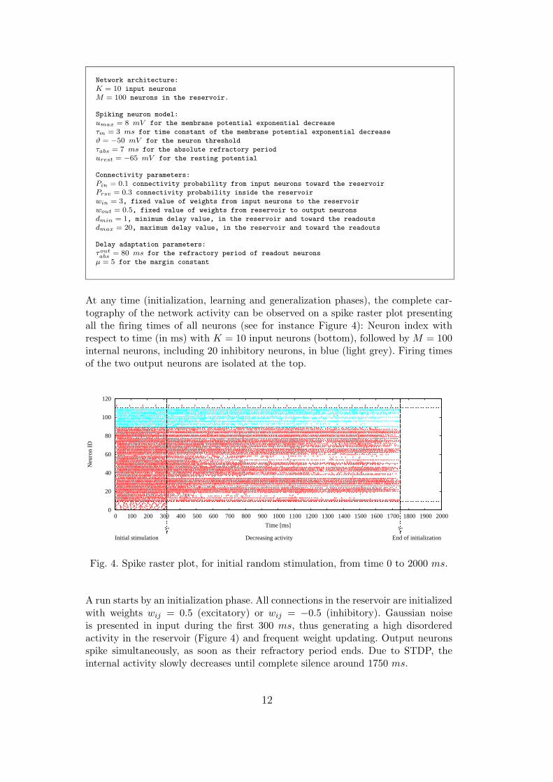
At any time (initialization, learning and generalization phases), the complete car-tography of the network activity can be observed on a spike raster plot presentingall the firing times of all neurons (see for instance Figure 4): Neuron index withrespect to time (in ms) with K = 10 input neurons (bottom), followed by M = 100internal neurons, including 20 inhibitory neurons, in blue (light grey). Firing timesof the two output neurons are isolated at the top.

0

20

40

60

80

100

120

0 100 200 300 400 500 600 700 800 900 1000 1100 1200 1300 1400 1500 1600 1700 1800 1900 2000

Neu

ron

ID

Time [ms]

Initial stimulation Decreasing activity End of initialization

Fig. 4. Spike raster plot, for initial random stimulation, from time 0 to 2000 ms.

A run starts by an initialization phase. All connections in the reservoir are initializedwith weights wij = 0.5 (excitatory) or wij = −0.5 (inhibitory). Gaussian noiseis presented in input during the first 300 ms, thus generating a high disorderedactivity in the reservoir (Figure 4) and frequent weight updating. Output neuronsspike simultaneously, as soon as their refractory period ends. Due to STDP, theinternal activity slowly decreases until complete silence around 1750 ms.

12

4.1.1 Learning

Afterwards, a learning phase is run, between times TL1 and TL2. Figure 5 presentstwo time slices of a learning run, with successive alternated presentations of the twoinput patterns that represent examples for class 1 and class 2 respectively. As canbe observed, the internal network activity quickly decreases and then stabilizes ona persistent alternative between two different spike-timing patterns (lasting slightlylonger than the time range of pattern presentation), one for each class. The learningperformance is a 100% success rate, even in experiments where the patterns to belearned are presented in random order.

0

20

40

60

80

100

120

2300 2400 2500 2600 2700 2800 2900 3000 3100 3200

0

20

40

60

80

100

120

8500 8600 8700 8800 8900 9000 9100

Fig. 5. Spike raster plots, for two time slices of a learning run, one just after TL1

(top) and the other a long time after activity has stabilized, until TL2 (bottom).

The evolution of the firing times of the two output neurons reflects the applicationof the delay adaptation algorithm. Starting from simultaneous firing, they slightlydissociate their responses, from a pattern presentation to the next, according to theclass corresponding to the input (top frame, Figure 5). In the bottom frame of thefigure, the time interval separating the two output spikes has become larger, due todelay adaptation, and is stable, since the margin µ has been reached. The internalactivity is quite invariant, except for occasional differences due to the still runningSTDP adaptation of weights. This point will be discussed later (Sections 4.1.3 and

13

6).

4.1.2 Generalization

Finally between TG1 and TG2 a generalization phase is run with noisy patterns:Each spike time occurs at t± η where t is the firing time of the corresponding inputneuron for the example pattern of the same class and η is some uniform noise. InFigure 6, two noise levels can be compared. Although the internal network activityis clearly disrupted, the classification performance remains good: Average successrate, on 100 noisy patterns of each class, is 96% for η = 4, when noisy patterns arepresented alternatively, class 2 after class 1, and still 81% for η = 8, where the inputpatterns are hard to discriminate by a human observer. We observed a slight effectof sequence learning: Only 91% and 73% success respectively for η = 4 and η = 8,when class 1 and class 2 are presented in random order.

0

20

40

60

80

100

120

18500 18600 18700 18800 18900 19000 19100 19200 18900 19000 19100 19200 19300 19400 19500 19600

Fig. 6. Spike raster plots, for two series of noisy patterns: η = 4 (top) and 8 (bottom).

We observe that the obtained margin between the two output firing times canbe higher or lower than µ. For each pattern, this margin could be exploited as aconfidence measure over the network answer. Moreover, most of the non-successfulcases are due to simultaneous firing of the two output neurons (in Figure 6, onlyone wrong order near the left of 18800 ms). Such ambiguous responses can beconsidered as “non-answers”, and could lead to define a subset of rejected patterns.Wrong order output spike-firing patterns are seldom, which attest the robustness ofthe learning algorithm.

The performance is increased and the sequence effect disappears when the marginconstant is set to a higher value. For µ = 8 instead of µ = 5, the generalizationsuccess rate reaches 100% for η = 4 and 90% for η = 8, for both an alternate or arandom presentation of the patterns. In the latter case, the error rate is only 0.3%and the 9.7% remaining cases are “non-answers”. This phenomenon could be usedas a criterion for tuning the margin hyper-parameter.

14

4.1.3 Weight Distributions

In order to illustrate the weight adaptation that occurs in the reservoir, Figures 7and 8 show respectively the distribution of excitatory and inhibitory weights (inabsolute value) quantized into 10 uniform segments of 0.1 and captured at differenttimes. The distribution at time 0 is not shown, as all the | wij | were initialized to0.5. Afterwards, it can be checked that weights are widely distributed in the range[wmin, wmax]. First, at the end of initialization phase, excitatory weights (Figure7) tend to be Gaussian around the original distribution (time 300 and 2000). Wehave measured that the average amount of time between two spikes during the first1700 ms corresponds to 8 ms. In the excitatory STDP temporal window (Figure 2,left), |∆W | in the range of 8 ms is comparable at both sides of 0, and thus explainsthis Gaussian redistribution. Then, during the learning phase, weights uniformlydistribute, mainly from 0 to 0.7, for instance at time 4000. Around 10000 ms,an equilibrium is reached since strong variations of weights no longer occur underthe influence of STDP. It can be thought that the causal order of firing has beencaptured inside the network. The distribution of weight values is approximately 50%very close to 0, other weights being decreasingly distributed from 0.1 to 0.7.

0

0.2

0.4

0.6

0.8

1

0 0.1 0.2 0.3 0.4 0.5 0.6 0.7 0.8 0.9 1

Rat

io fo

r ea

ch s

lice

0

0.2

0.4

0.6

0.8

1

0 0.1 0.2 0.3 0.4 0.5 0.6 0.7 0.8 0.9 1 0

0.2

0.4

0.6

0.8

1

0 0.1 0.2 0.3 0.4 0.5 0.6 0.7 0.8 0.9 1 0

0.2

0.4

0.6

0.8

1

0 0.1 0.2 0.3 0.4 0.5 0.6 0.7 0.8 0.9 1

Fig. 7. Excitatory weights distribution at time 300, 2000, 4000, 10000 ms.

Let us now consider inhibitory weights in Figure 8. As the initial internal activityis strong, the weights are modified in a very short time range. Indeed, looking attime 300 (Figure 8, left) we see that weights have already nearly all migrated toan extremal value (close to −1). This surprising violent migration can as well beexplained by the inhibitory STDP function, where close spikes in an inhibitorysynapse produce a strong weight potentiation (see Figure 2, right). A high activitystrongly potentiates the inhibitory synapses that, in turn, slow down the activity,thus playing a regulatory role. After the initial stimulation stopped, weights begin toredistribute as the reservoir activity slows down. From then on, weight distributionhas reached a state that slightly evolves, until time 10000, and stays very stableuntil time 17000 (end of learning phase).

0

0.2

0.4

0.6

0.8

1

0 0.1 0.2 0.3 0.4 0.5 0.6 0.7 0.8 0.9 1

Rat

io fo

r ea

ch s

lice

0

0.2

0.4

0.6

0.8

1

0 0.1 0.2 0.3 0.4 0.5 0.6 0.7 0.8 0.9 1 0

0.2

0.4

0.6

0.8

1

0 0.1 0.2 0.3 0.4 0.5 0.6 0.7 0.8 0.9 1 0

0.2

0.4

0.6

0.8

1

0 0.1 0.2 0.3 0.4 0.5 0.6 0.7 0.8 0.9 1

Fig. 8. Distribution of | wij | for inhibitory weights at time 300, 2000, 4000,10000 ms.

Note that, due to the multiplicative [36] application of STDP temporal windows(Section 3.1), the weights are never strictly equal to wmin or wmax. Experiments

15

show that they do not saturate toward extremal values. This observation confirmsthe interest of multiplicative STDP: The effect on the weight distribution is com-parable to the result of combining IP (Intrinsic Plasticity) and classic STDP, thathas been proved to enhance the performance and the network stability [21].

In [15] Jaeger claims that the spectral radius of the weight matrix must be smallerthan 1. This point has been widely discussed and confirmed by studies on thenetwork dynamics proving that a spectral radius close to 1 is an optimal value.However we share the opinion of Verstraeten et al. [49] who claim that “for spikingneurons it has no influence at all”. In [43] Steil shows that a learning rule based on IPhas the effect to expand the eigenvalues away from the center of the unit disk. On fewmeasurements, we observed a converse effect with our learning rule and with spectralradii higher than 1, e.g. λ = 8.7 for the initial weight matrix and λ = 2.3 after alearning phase of 20000 ms. This point remains to be more deeply investigated,both through more experimental measurements and a theoretical study.

4.2 OCR on the USPS Database

The patterns of the USPS dataset 5 [13] consist of 256 dimensional vectors of realnumbers between 0 and 2, corresponding to 16 ∗ 16 pixels gray-scale images ofhandwritten digits (examples on Figure 9). They are presented to the network intemporal coding: The higher the numerical value, the darker the pixel color, theearlier the spike firing of the corresponding input neuron, inside a time window ofT = 20 ms. Hence, the significant part of the pattern (i.e. the localization of theblack pixels) is presented first to the network, which is an advantage of temporalprocessing compared to usual methods that scan the image matrix of pixels lineafter line.

Fig. 9. USPS patterns examples: 1, 5, 8, 9 digits.

For this task, the neuron model constants and network hyper-parameters have beenset as follows:



M = 100 neurons in the reservoir



All other parameters are the same as parameters of Section 4.1.

5 http://www-stat-class.stanford.edu/∼tibs/ElemStatLearn/data.html

16

4.2.1 Two-Class Setting

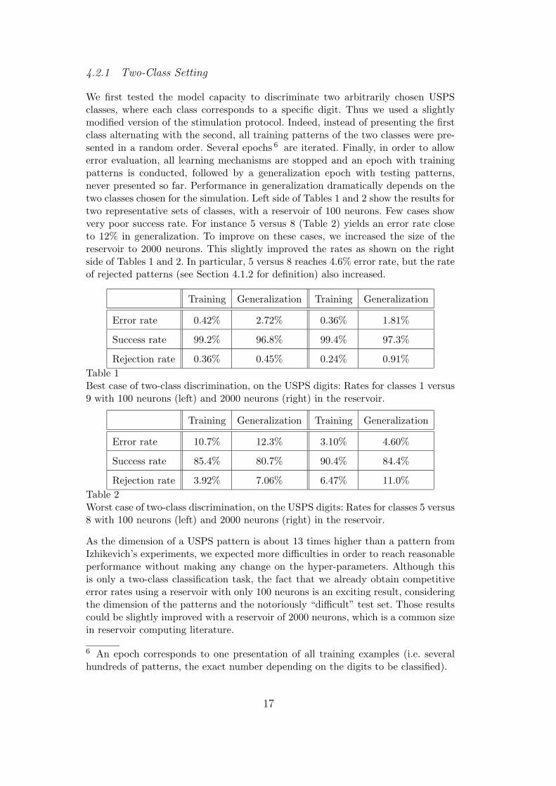
We first tested the model capacity to discriminate two arbitrarily chosen USPSclasses, where each class corresponds to a specific digit. Thus we used a slightlymodified version of the stimulation protocol. Indeed, instead of presenting the firstclass alternating with the second, all training patterns of the two classes were pre-sented in a random order. Several epochs 6 are iterated. Finally, in order to allowerror evaluation, all learning mechanisms are stopped and an epoch with trainingpatterns is conducted, followed by a generalization epoch with testing patterns,never presented so far. Performance in generalization dramatically depends on thetwo classes chosen for the simulation. Left side of Tables 1 and 2 show the results fortwo representative sets of classes, with a reservoir of 100 neurons. Few cases showvery poor success rate. For instance 5 versus 8 (Table 2) yields an error rate closeto 12% in generalization. To improve on these cases, we increased the size of thereservoir to 2000 neurons. This slightly improved the rates as shown on the rightside of Tables 1 and 2. In particular, 5 versus 8 reaches 4.6% error rate, but the rateof rejected patterns (see Section 4.1.2 for definition) also increased.

Training Generalization Training Generalization

Error rate 0.42% 2.72% 0.36% 1.81%

Success rate 99.2% 96.8% 99.4% 97.3%

Rejection rate 0.36% 0.45% 0.24% 0.91%

Table 1Best case of two-class discrimination, on the USPS digits: Rates for classes 1 versus9 with 100 neurons (left) and 2000 neurons (right) in the reservoir.

Training Generalization Training Generalization

Error rate 10.7% 12.3% 3.10% 4.60%

Success rate 85.4% 80.7% 90.4% 84.4%

Rejection rate 3.92% 7.06% 6.47% 11.0%

Table 2Worst case of two-class discrimination, on the USPS digits: Rates for classes 5 versus8 with 100 neurons (left) and 2000 neurons (right) in the reservoir.

As the dimension of a USPS pattern is about 13 times higher than a pattern fromIzhikevich’s experiments, we expected more difficulties in order to reach reasonableperformance without making any change on the hyper-parameters. Although thisis only a two-class classification task, the fact that we already obtain competitiveerror rates using a reservoir with only 100 neurons is an exciting result, consideringthe dimension of the patterns and the notoriously “difficult” test set. Those resultscould be slightly improved with a reservoir of 2000 neurons, which is a common sizein reservoir computing literature.

6 An epoch corresponds to one presentation of all training examples (i.e. severalhundreds of patterns, the exact number depending on the digits to be classified).

17

4.2.2 Multi-Class Setting

A few simulations have been performed on the whole 10 classes of the USPS dataset.Several experimental tunings of the hyper-parameters over the training set led tothe following values :



M = 2000 neurons in the reservoir

10 readout neurons, instead of 2

Spiking neuron model:

τm = 20 ms for time constant of the membrane potential exponential decrease



Prsv = 0.0145 connectivity probability inside the reservoir

wOUT = 0.02, fixed value of weights from reservoir to output neurons

dmax = 100, maximum delay value, only toward the readouts

All other parameters are the same as parameters of Section 4.1.

We let the simulation go through 20 training epochs before evaluating the rates onthe train and test sets. We obtain an error rate of 8.8% on the training set thatjumps to 13.5% on the testing set. Although the performance is not yet competitivewith the best well-tuned machine learning approaches that nearly reach 2% in testerror (see [20] for a review of performance on the multi-class USPS dataset), themulti-timescale learning rule proves to behave correctly on real-world data. Weemphasize that our error rates have been reached after few tunings w.r.t. the sizeand complexity of the database. First, increasing the size of the reservoir from 100 to2000 neurons yielded improved performance. Note that setting τm (see Section 2.1)to a larger value (i.e. 20, instead of 3), in the readout neurons only, induces a slowerdecrease of their membrane potential. The neurons are thus tuned to behave asintegrators [33].

Training Generalization

Error rate 8.87% 13.6%

Success rate 85.0% 79.1%

Rejection rate 6.13% 7.32%

Table 3Rates for all 10 classes of USPS dataset

Another key point was to set a wider range of possible delay values for the readoutconnections. Thus, allowing the connections to be set in [1, 100] instead of [1, 20]also improved the success rate, and reduced the rejection rate. This let us think thatthe discretization of the delays is too low to avoid coincidence of readout spikes. Inorder to circumvent this effect, a test has been performed with a different time step:0.1 ms instead of 1 ms, on a reservoir of 200 neurons. The result has been a 7%increase of the generalization success rate, mainly coming from a decrease (−5.5%)of rejected patterns.

18

Although the multi-class case needs further investigation, we consider these pre-liminary results and observations as very encouraging. Hyper-parameters (mainlythe reservoir size and the connectivity probabilities) have to be tuned. Hence theirinteractions with the neuron model constants have to be controlled in order to keepa convenient level of activity inside the reservoir. Understanding more deeply theactivity and the effects of modifying connectivity in the reservoir will hopefully helpto improve the classification performance. Nevertheless, the concept is validated, asconfirmed by the analysis of the model behavior presented in the next two sections.

5 Polychronization

5.1 Cell Assemblies and Synchrony

A cell assembly can be defined as a group of neurons with strong mutual excitatoryconnections. Since a cell assembly tends to be activated as a whole once a subset ofits cells are stimulated, it can be considered as an operational unit in the brain. In-herited from Hebb, current thoughts about cell assemblies are that they could play arole of “grandmother neural groups” as basis of memory encoding, instead of the olddebated notion of “grandmother cell”, and that material entities (e.g. a book, a cup,a dog) and, even more, mental entities (e.g. ideas or concepts) could be representedby different cell assemblies. However, although reproducible spike-timing patternshave been observed in many physiological experiments, the way these spike-timingpatterns, at the millisecond scale are related to high-level cognitive processes is stillan open question.

Deep attention has been paid to synchronization of firing times for subsets of neu-rons inside a network. The notion of synfire chain [2,11], a pool of neurons firingsynchronously, can be described as follows: If several neurons have a common post-synaptic neuron Nj and if they fire synchronously then their firing will superimposein order to trigger Nj . However, the argument falls down if the axonal transmissiondelays are to be considered, since the incoming synapses of Nj have no reason toshare a common delay value. Synchronization appears to be a too restrictive notionwhen it comes to grasp the full power of cell assemblies processing. This point hasbeen highlighted by Izhikevich [14] who proposes the notion of polychronization.

5.2 Polychronous Groups

Polychronization is the ability of an SNN to exhibit reproducible time-locked but notsynchronous firing patterns with millisecond precision, thus giving a new light to thenotion of cell assembly. Based on the connectivity between neurons, a polychronous

group (PG) is a possible stereotypical time-locked firing pattern. For example, in

19

Figure 10, if we consider a delay of 15 ms from neuron N1 to neuron N2, and a delayof 8 ms from neuron N3 to neuron N2, then neuron N1 emitting a spike at time tand neuron N3 emitting at time t+7 will trigger a spike firing by neuron N2 at timet+15 (supposing two coincident incoming spikes are enough to make a neuron fire).Since neurons of a polychronous group have matching axonal conduction delays,the group can be the basis of a reproducible spike-timing pattern: Firing of the firstfew neurons with the right timing is enough to activate most of the group (with atolerance of 1 ms jitter on spike-timing).

8 ms

15 ms

N3

N2

N1

Time [ms]

Fig. 10. Example of two triggering neurons giving rise to a third one firing.

Since any neuron can be activated within several PGs, at different times (e.g. neuron76 in Figure 11), the number of coexisting PGs in a network can be much greaterthan its number of neurons, thus opening possibility of huge memory capacity. Allthe potential PGs in a reservoir network of M neurons, depending on its topologyand the values of the internal transmission delays (that are kept fixed), can be enu-merated using a greedy algorithm of complexity O(M2+F ), where F is the numberof triggering neurons to be considered. In the reservoir used for experiments onIzhikevich’s patterns (Section 4.1), we have referenced all the possible polychronousgroups inherent in the network topology, with F = 3 triggering neurons (see Fig-ure 11 for examples). We have detected 104 potentially activatable PGs in a networkof M = 100 neurons. In similar conditions, the number of PGs already overcomes3000 in a network of M = 200 neurons.

0

20

40

60

80

100

0 5 10 15 20 25 30

Neu

rons

t [ms]

Triggering neurons: 19,55,76, with

timing pattern (0,11,13)

0

20

40

60

80

100

0 5 10 15 20 25 30

Neu

rons

t [ms]

Triggering neurons: 21,52,76, with

timing pattern (7,7,0)

Fig. 11. Examples of polychronous groups: PG 50 and PG 51. Starting from threeinitial triggering neurons, further neurons of the group can be activated, in chain,with respect to the spike-timing patterns represented on the diagrams.

Our model proposes a way to confirm the link between an input presentation andthe activation of persistent spike-timing patterns inside the reservoir, and the waywe take advantage of polychronous groups for supervising the readout adaptationis explained in the next section.

20

6 Reservoir Internal Dynamics

Since the number of polychronous groups increases very rapidly when the reservoirsize grows (cf. Section 5.2), the dynamical behavior of the network has been deeplyexamined only for the two-class experiments on Izhikevich’s patterns, where thenetwork size remains small (104 PGs only). All along the initialization, learningand generalization phases, the reservoir internal dynamics has been analyzed interms of actually activated polychronous groups. Figure 12 presents the evolutionof polychronous groups activation in experiments. The evolution of activated PGs isentirely governed by STDP, the only adaptation process acting inside the reservoirnetwork.

0 5

10 15 20 25 30 35 40 45 50 55 60 65 70 75 80 85 90 95

100 105

0 1000 2000 3000 4000 5000 6000 7000 8000 9000 10000 11000 12000 13000 14000 15000 16000 17000 18000 19000 20000

Pol

ychr

onou

s gr

oups

t [ms]

Initial stimulation Training Testing

Fig. 12. Evolution of polychronous groups activation during the initialization, learn-ing and generalization phases of experiments reported in Section 4.1, with alternateclass input presentations. Note that, in this figure, the y-axis represents the PGindices and no longer the neuron indices, as was the case on spike raster plots.

We observe that many PGs are frequently activated during the initial random stim-ulation that generates a strong disordered activity in the internal network (before2000 ms). At the beginning of the learning phase (which goes from 2000 ms to17000 ms), many groups are activated, and then, roughly after 5000 ms, the activa-tion landscape becomes very stable. As anticipated, only a few specific polychronousgroups continue to be busy. Small subsets of PGs can be associated to each class:Groups 3, 41, 74, 75 and 83, switching to 85, fire for class 1, whereas groups 12, 36,95, sometimes 99, and 49, switching to 67, fire for class 2. During the generalizationphase (after 17000 ms), the main and most frequently activated groups are thoseidentified during the learning phase. This observation supports the hypothesis thatpolychronous groups have become representative of the class encoding realized bythe multi-scale learning rule.

Several interesting observations can be reported. As noticed by Izhikevich, thereexist groups that start to be activated only after a large number of repeated stim-

21

ulations (e.g. 41, 49, 67 and 85), whereas some other groups stop their activationafter a while (e.g. 5 and some others [active until 4000/5000 ms only], 49, 70, 83 and99 [later]). We can also observe that PGs specialize for one particular class (laterthan 8000 ms) instead of answering for both of them, as they did first (mainly from2000 to 5000 ms).

0

20

40

60

80

100

60 65 70 75 80 85 90 95 100

Per

cent

age

of a

ctiv

atio

n

# polychronous groups

activations in response to class 1activations in response to class 2

0

20

40

60

80

100

60 65 70 75 80 85 90 95 100

Per

cent

age

of a

ctiv

atio

n

# polychronous groups


Fig. 13. Activation ratio from 2000 to 5000ms, and then from 8000 to 11000ms.

An histogram representation of a subset of the 104 PGs (Figure 13) better pointsout the latter phenomenon. A very interesting case is the polychronous group num-ber 95 which is first activated by both example patterns, and then (around time7500 ms) stops responding for class 1, thus specializing its activity for class 2. Suchphenomenon validates that synaptic plasticity provides the network with valuableadaptability and highlights the importance of combining STDP with delay learning.

10 15 20 25 30 35 40 45 50 55 60 65 70 75 80 85 90

17000 10000 2000 0

Neu

rons

t [ms]

Initial stimulation Training Testing

Fig. 14. The 80 excitatory neurons of the reservoir have been marked by a red(black) ”+” for class 1 or a blue (light grey) ”x” for class 2 each time they play therole of pre-synaptic neuron of a triggering connection producing a readout delaychange.

The influence of active PGs on the learning process can also be exhibited. We haverecorded (Figure 14) the indices of the pre-synaptic neurons responsible for theapplication of the output delay update rule, at each iteration where the examplepattern was not yet well classified (cf. Algorithm 1, Section 3.2). For instance,neuron #42, which is repeatedly responsible for delay adaptation, is one of the

22

triggering neurons of the polychronous group number 12, activated for class 2 duringthe training phase. One will notice that delay adaptation stops before the learningphase is over, which means the learning process is already efficient around 10000 ms.Such a control could be implemented in the proposed algorithms, as a heuristic for abetter stopping criterion (rather than the current “until a given maximum learningtime is over”).

0

5

10

15

20

25

30

0 1 2 3 4 5 6 7 8 9 10 11 12 13 14 15 16 17 18 19 20 21 22 23 24 25 26 27 28 29 30 31 32 33 34 35 36 37 38 39 40 41 42 43 44 45 46 47 48 49 50 51 52 53 54 55 56 57 58 59 60 61 62 63 64 65 66 67 68 69 70 71 72 73 74 75 76 77 78 79 80 81 82 83 84 85 86 87 88 89 90 91 92 93 94 95 96 97

Pou

rcen

tage

of a

ctiv

atio

ns

Poly. groups IDs


0

5

10

15

20

25

30

0 1 2 3 4 5 6 7 8 9 10 11 12 13 14 15 16 17 18 19 20 21 22 23 24 25 26 27 28 29 30 31 32 33 34 35 36 37 38 39 40 41 42 43 44 45 46 47 48 49 50 51 52 53 54 55 56 57 58 59 60 61 62 63 64 65 66 67 68 69 70 71 72 73 74 75 76 77 78 79 80 81 82 83 84 85 86 87 88 89 90 91 92 93 94 95 96 97

Pou

rcen

tage

of a

ctiv

atio

ns

Poly. groups IDs


Fig. 15. Activation ratio of PGs in a 100 neurons reservoir, for two-class discrimi-nation of USPS digits 1 versus 9, during the 1st (left) and the 5th (right) epochs.

Figure 15 confirms the selection of active polychronous groups during the learningprocess, even on complex data. Although the phenomenon is less precise, due tothe high variability of USPS patterns inside each class, it still remains observable:After only 5 epochs of the learning phase, the activity of many PGs has vanishedand several of them are clearly specialized for one class or the other.

7 Conclusion

We have proposed a new model for Reservoir Computing, based on a multi-timescalelearning mechanism for adapting a Spiking Neuron Network to a classification task.The proof of concept is based on the notion of polychronization. Under the effect ofsynaptic plasticity (STDP), the reservoir network dynamics induces the emergenceof a few active polychronous groups specific to the patterns to be discriminated. Thedelay adaptation mechanism of the readout neurons makes them capture the internalactivity so that the target class neuron fires before the other ones, with an enforcedtime delay margin. Adaptation to the task at hand is based on biological inspiration.The delay learning rule is computationally easy to implement and gives a wayto supervise the overall process. Performance on two-class discrimination tasks isreasonably good, even with a small size of reservoir network, on notoriously difficultpatterns. Deeper investigation on the interactions between the hyper-parameterswould help to improve the performance. A first track consists in running the reservoirsimulation with a smaller time step for large and noisy databases.

While the notion of margin is important in modern machine learning literature,it needs to be paired with some form of regularization. We thus intend to alsoexplore ways to implement a regularization process in Reservoir Computing in

23

the near future. Another perspective is to adapt the method to regression tasksor time series prediction in order to stronger exploit the opportunity of temporalprocessing in the reservoir. In future work we will test our classification task onother reservoir computing models in order to compare the results of our model tothose of the literature. We will use the Reservoir Computing Toolbox available athttp://www.elis.ugent.be/rct [38].

Acknowledgement

The authors acknowledge David Meunier for precious help and clever advice aboutthe most pertinent way to implement STDP and anonymous reviewers for valuablesuggestions.

References

[1] L. Abbott, S. Nelson, Synaptic plasticity: taming the beast, NatureNeuroscience 3 (2000) 1178–1183.

[2] M. Abeles, Corticonics: Neural Circuits of the Cerebral Cortex, CambridgePress, 1991.

[3] G.-q. Bi, M.-m. Poo, Synaptic modification in cultured hippocampal neurons:Dependence on spike timing, synaptic strength, and polysynaptic cell type, J.of Neuroscience 18 (24) (1998) 10464–10472.

[4] S. Bohte, J. Kok, H. La Poutre, Spikeprop: Error-backpropagation in temporallyencoded networks of spiking neurons, Neurocomputing 48 (2002) 17–37.

[5] S. Bohte, M. Mozer, Reducing the variability of neural responses:A computational theory of spike-timing-dependent plasticity., NeuralComputation 19 (2) (2007) 371–403.

[6] V. Braitenberg, A. Schuz, Anatomy of the cortex: Statistics and geometry,Springer-Verlag, 1991.

[7] N. Butko, J. Triesch, Learning sensory representations with intrinsic plasticity,Neurocomputing 70 (2007) 1130–1138.

[8] G. Chechik, Spike-timing dependent plasticity and relevant mutual informationmaximization, Neural Computation 15 (7) (2003) 1481–1510.

[9] G. Daoudal, D. Debanne, Long-term plasticity of intrinsic excitability: Learningrules and mechanisms, Learning and Memory 10 (2003) 456–465.

[10] N. Desai, L. Rutherford, G. Turrigiano, Plasticity in the intrinsic excitabilityof cortical pyramidal neurons, Nature Neuroscience 2 (6) (1999) 515–520.

24

[11] M. Diesmann, M.-O. Gewaltig, A. Aertsen, Stable propagation of synchronousspiking in cortical neural networks, Nature 402 (1999) 529–533.

[12] W. Gerstner, W. Kistler, Spiking Neuron Models: Single Neurons, Populations,Plasticity, Cambridge University Press, 2002.

[13] T. Hastie, R. Tibshirani, J. Friedman, The elements of statistical learning,Springer-Verlag, 2001.

[14] E. Izhikevich, Polychronization: Computation with spikes, Neural Computation18 (2) (2006) 245–282.

[15] H. Jaeger, The “echo state” approach to analysing and training recurrent neuralnetworks, Tech. Rep. TR-GMD-148, German National Research Center forInformation Technology (2001).

[16] H. Jaeger, Adaptive nonlinear system identification with Echo State Networks,in: S. Becker, S. Thrun, K. Obermayer (eds.), NIPS*2002, Advances in NeuralInformation Processing Systems, vol. 15, MIT Press, 2003.

[17] H. Jaeger, W. Maass, J. Principe, Special issue on echo state networks andliquid state machines (editorial), Neural Networks 20 (3) (2007) 287–289.

[18] E. Kandell, J. Schwartz, T. Jessell, Principles of Neural Science, 4th edition,McGraw-Hill, 2000.

[19] R. Kempter, W. Gerstner, J. L. van Hemmen, Hebbian learning and spikingneurons, Physical Review E 59 (4) (1999) 4498–4514.

[20] D. Keysers, R. Paredes, H. Ney, E. Vidal, Combination of tangent vectorsand local representations for handwritten digit recognition, in: SPR 2002,International Workshop on Statistical Pattern Recognition, Windsor, Ontario,Canada, 2002.

[21] A. Lazar, G. Pipa, J. Triesch, Fading memory and time series prediction inrecurrent networks with different forms of plasticity, Neural Networks 20 (3)(2007) 312–322.

[22] W. Maass, Networks of spiking neurons: The third generation of neural networkmodels, Neural Networks 10 (1997) 1659–1671.

[23] W. Maass, On the relevance of time in neural computation and learning,Theoretical Computer Science 261 (2001) 157–178, (extended version of ALT’97,in LNAI 1316:364-384).

[24] W. Maass, T. Natschlager, Networks of spiking neurons can emulate arbitraryHopfield nets in temporal coding, Network: Computation in Neural Systems8 (4) (1997) 355–372.

[25] W. Maass, T. Natschlager, H. Markram, Real-time computing without stablestates: A new framework for neural computation based on perturbations, NeuralComputation 14 (11) (2002) 2531–2560.

25

[26] W. Maass, M. Schmitt, On the complexity of learning for a spiking neuron, in:COLT’97, Conf. on Computational Learning Theory, ACM Press, 1997.

[27] W. Maass, M. Schmitt, On the complexity of learning for spiking neurons withtemporal coding, Information and Computation 153 (1999) 26–46.

[28] H. Markram, J. Lubke, M. Frotscher, B. Sakmann, Regulation of synapticefficacy by coincidence of postsynaptic APs and EPSPs, Science 275 (1997)213–215.

[29] D. Meunier, H. Paugam-Moisy, Evolutionary supervision of a dynamical neuralnetwork allows learning with on-going weights, in: IJCNN’2005, Int. Joint Conf.on Neural Networks, IEEE–INNS, 2005.

[30] T. Natschlager, B. Ruf, Spatial and temporal pattern analysis via spikingneurons, Network: Comp. Neural Systems 9 (3) (1998) 319–332.

[31] D. Norton, D. Ventura, Preparing more effective liquid state machines usinghebbian learning, in: IJCNN’2006, Int. Joint Conf. on Neural Networks, IEEE-INNS, 2006.

[32] T. Nowotny, V. Zhigulin, A. Selverston, H. Abardanel, M. Rabinovich,Enhancement of synchronization in a hibrid neural circuit by Spike-Time-Dependent Plasticity, The Journal of Neuroscience 23 (30) (2003) 9776–9785.

[33] H. Paugam-Moisy, Spiking neuron networks: A survey, IDIAP-RR 11, IDIAP(2006).

[34] H. Paugam-Moisy, R. Martinez, S. Bengio, A supervised learning approachbased on STDP and polychronization in spiking neuron networks,Tech. Rep. 54, IDIAP, http://www.idiap.ch/publications/paugam-esann-2007.bib.abs.html (october 2006).

[35] J.-P. Pfister, T. Toyoizumi, D. Barber, W. Gerstner, Optimal spike-timingdependent plasticity for precise action potential firing in supervised learning,Neural Computation 18 (6) (2006) 1318–1348.

[36] J. Rubin, D. Lee, H. Sompolinsky, Equilibrium properties of temporallyassymmetric Hebbian plasticity, Physical Review Letters 89 (2) (2001) 364–367.

[37] M. Schmitt, On computing boolean functions by a spiking neuron, Annals ofMathematics and Artificial Intelligence 24 (1998) 181–191.

[38] B. Schrauwen, D. Verstraeten, J. Van Campenhout, An overview of reservoircomputing: theory, applications and implementations, in: M. Verleysen (ed.),ESANN’2007, Advances in Computational Intelligence and Learning, 2007.

[39] W. Senn, M. Schneider, B. Ruf, Activity-dependent development of axonal anddendritic delays, or, why synaptic transmission should be unreliable, NeuralComputation 14 (2002) 583–619.

26

[40] J. Sima, J. Sgall, On the nonlearnability of a single spiking neuron, NeuralComputation 17 (12) (2005) 2635–2647.

[41] W. Singer, Neural synchrony: A versatile code for the definition of relations?,Neuron 24 (1999) 49–65.

[42] J. Steil, Backpropagation-decorrelation: Online recurrent learning with O(N)complexity, in: IJCNN’2004, Int. Joint Conf. on Neural Networks, IEEE–INNS,2004.

[43] J. Steil, Online reservoir adaptation by intrinsic plasticity for backpropagation-decorrelation and echo state learning, Neural Networks 20 (3) (2007) 353–364.

[44] H. Swadlow, Physiological properties of individual cerebral axons studied invivo for as long as one year, Journal of Neurophysiology 54 (1985) 1346–1362.

[45] H. Swadlow, Monitoring the excitability of neocortical efferent neurons to directactivation by extracellular current pulses, J. Neurophysiology 68 (1992) 605–619.

[46] T. Toyoizumi, J.-P. Pfister, K. Aihara, W. Gerstner, Generalized Bienenstock- Cooper - Munro rule for spiking neurons that maximizes informationtransmission, Proc. Natl. Acad. Sci. 102 (14) (2005) 5239–5244.

[47] J. Triesch, A gradient rule for the plasticity of a neuron’s intrinsic excitability,in: ICANN’05, Int. Conf. on Artificial Neural Networks, 2005.

[48] V. Vapnik, Statistical learning theory, Wiley, 1998.

[49] D. Verstraeten, B. Schrauwen, M. D’Haene, D. Stroobandt, An experimentalunification of reservoir computing methods, Neural Networks 20 (3) (2007) 391–403.

[50] M. Wardermann, J. Steil, Intrinsic plasticity for reservoir learning algorithms,in: M. Verleysen (ed.), ESANN’2007, Advances in Computational Intelligenceand Learning, 2007.

[51] M. Woodin, K. Ganguly, M. Poo, Coincident pre- and postsynaptic activitymodifies gabaergic synapses by postsynaptic changes in CL-transporter activity,Neuron 39 (5) (2003) 807–820.

27

delay learning and polychronization for reservoir...

Documents