delft university of technology de faculteit... · can be used to approximate rst integrals. not...
TRANSCRIPT

DELFT UNIVERSITY OF TECHNOLOGY
REPORT 03-04
On Approximations of First Integrals
for a Strongly Nonlinear Forced Oscillator
S.B. Waluya and W.T. van Horssen
ISSN 1389-6520
Reports of the Department of Applied Mathematical Analysis
Delft 2003
Copyright 2000 by Department of Applied Mathematical Analysis, Delft, The Netherlands.
No part of the Journal may be reproduced, stored in a retrieval system, or transmitted, inany form or by any means, electronic, mechanical, photocopying, recording, or otherwise,without the prior written permission from Department of Applied Mathematical Analysis,Delft University of Technology, The Netherlands.

On Approximations of First Integrals for a Strongly
Nonlinear Forced Oscillator
S. B. Waluya∗ and W.T. van Horssen
Department of Applied Mathematical Analysis,
Faculty of Information Technology and Systems, Delft University of Technology,
Mekelweg 4, 2628 CD Delft,
The Netherlands
([email protected], [email protected])
Abstract
In this paper a strongly nonlinear forced oscillator will be studied. It will beshown that the recently developed perturbation method based on integrating factorscan be used to approximate first integrals. Not only approximations of first integralswill be given, but it will also be shown how, in a rather efficient way, the existenceand stability of time-periodic solutions can be obtained from these approximations.In addition phase portraits, Poincare-return maps, and bifurcation diagrams for aset of values of the parameters will be presented. In particular the strongly nonlinear
forced oscillator equation X+X+λX3 = ε(
δX − βX3 + γX cos(2t))
will be studied
in this paper. It will be shown that the presented perturbation method not only canbe applied to a weakly nonlinear oscillator problem (that is, when the parameterλ = O(ε)) but also to a strongly nonlinear problem (that is, when λ = O(1)). Themodel equation as considered in this paper is related to the phenomenon of gallopingof overhead power transmission lines on which ice has accreted.
Keywords: Integrating factor, integrating vector, first integral, perturbation method,asymptotic approximation of first integral, periodic solution, strongly nonlinear forcedoscillator.
∗On leave from Mathematics Department, Semarang State University, Indonesia
1

APPROXIMATIONS OF FIRST INTEGRALS FOR NONLINEAR OSCILLATOR 2
1 Introduction
In this paper it will be shown how the perturbation method based on integrating vectorscan be applied to the following non-autonomous equation
X +dU(X)
dX= εf(X, X, t), (1.1)
where U(X) is the potential energy of the unperturbed (that is, ε = 0), nonlinear oscillator,where X = X(t), X = dX
dt, where ε is a small parameter satisfying 0 < ε � 1, and where
f is a sufficiently smooth function. Many classical perturbation methods have been usedto approximate analytically the solution of the weakly nonlinear problem (1.1), that is,
when dU(X)dX
in (1.1) is linear in X. However, when dU(X)dX
is non-linear in X most of theperturbation methods can not be applied to construct approximations of the solutions.In this paper it will be shown that the perturbation method based on integrating factorscan be applied to a class of non-autonomous nonlinear equations as described by (1.1). In
particular equation (1.1) with dU(X)dX
= X +λX3 and f(X, X, t) = δX − βX3 + γX cos(ωt)will be studied in detail in this paper. The existence and stability of time-periodic solutionswill be investigated. Bifurcation diagrams will be presented, and the dynamics of theoscillator as described by
X +X + λX3 = ε(
δX − βX3 + γX cos(ωt))
(1.2)
will be studied in this paper. In (1.2) it is assumed that the parameter λ is positive, thatis, it is assumed that the oscillator is attached to hard, nonlinear springs. The parametersδ > 0, β > 0, γ 6= 0, and ω are assumed to be constants independent of ε. The oscillatorequation (1.2) originates from the following system of ODEs
Y + ω21Y = ε
[
−a1,0Y + a2,0Y2 + a0,2X
2]
,
X + ω22X + λX3 = ε
[
b0,1X − b1,1Y X − b0,3X3]
,
(1.3)
which is a simple model for the flow-induced vibrations of a cable in a windfield. System(1.3) with λ = 0 or λ = O(ε) has been derived by Van der Beek in [2, 3]. The coefficientsa1,0, a2,0, a0,2, b0,1, b1,1, and b0,3 depend on the quasi-static drag and lift forces acting on aconductor line in a uniform windfield. System (1.3) can be considered to be an oscillatorwith two degrees of freedom which describes flow-induced vibration of cables in a windfield.The displacement of the cable in vertical direction (that is, perpendicular to the windflow)is described by X(t), and the displacement of the cable in horizontal direction (that is, inthe direction of the windflow) is given by Y (t). For more (and complete) details the readeris referred to [2, 3, 18]. It is well-known that galloping of conductor lines is an almostpurely vertical oscillation of these lines. Based upon the results as obtained in [2, 3, 13]which confirm this vertical oscillation it is now assumed that the oscillator will oscillate in

APPROXIMATIONS OF FIRST INTEGRALS FOR NONLINEAR OSCILLATOR 3
an almost vertical direction and that Y (t) = A cos(ω1t). In this way system (1.3) can bereduced to
X + ω22X + λX3 = ε
(
b0,1X − b1,1A cos(ω1t)X − b0,3X3)
. (1.4)
For small values of λ (that is, for λ = O(ε)) an interesting internal resonance for system(1.3) is ω1 : ω2 = 2 : 1. This case for instance has been studied in [2, 3]. In this paperit is also assumed that ω1 : ω2 = 2 : 1 when λ = O(1). After some elementary rescalingsin (1.4) equation (1.2) is finally obtained with ω = 2. In particular we will be interestedin the existence and stability of (order 1) periodic solutions of equation (1.2). Manyresearchers investigated extensively the behavior of the solutions of equations of the type(1.1). For instance, Nayfeh and Mook [1], Belhaq and Houssni [8] and others investigated
the steady-state (periodic) solutions of the weakly nonlinear equation (1.1) with dU(X)dX
=
ω20(1 + h cos(νt))X and f(X, X, t) = −αX − βX2 − ξX3 + γ cos(ωt) using a generalized
averaging method or a multiple time-scales perturbation method. For β = 0, h = 0 Limaand Pettini [10] studied the control of chaos in a periodically forced oscillator. They showedanalytically that a small nonlinear parametric perturbation can suppress chaos. Again byusing a multiple time-scales perturbation method Burton and Rahman [17] studied the
response of a weakly nonlinear oscillator as described by equation (1.1) with dU(X)dX
= mX
and f(X, X, t) = −2ηX − g(X) + 2P cos(ωt), where g(X) is an odd nonlinear function,and where m is an integer which may be either -1, 0, or 1. Roy [11] used an elliptic
averaging method to investigate (1.1) with dU(X)dX
= αX + γX3 and f(X, X, t) = −βX +
F cos(ωt). Brothers and Haberman [5] also studied (1.1) with f(X, X, t) = −h(X, X) +γ cos(2πωt), where h is a purely dissipative perturbation (h is odd in X) by using averagingand matching techniques. Higher-order averaging techniques based on Lie transforms havebeen used by Yagasaki and Ichikawa [6] to study weakly nonlinear equations like (1.1) withf(X, X, t) = −δX−βX2−αX3+γ cos(ωt). Van Horssen [20, 21] studied a weakly nonlinearDuffing equation (1.1) with f(X, X, t) = −aX − bX3 + c cos(t) using the perturbationmethod based on integrating factors and multiple time-scales. In this paper it will beshown that for the weakly non-autonomous and weakly nonlinear equation (1.2) exactlythe same results can be obtained as by applying the classical perturbation techniques(such as averaging, multiple time-scales, Poincare-Lindstedt or others). However, for thestrongly nonlinear equation (1.2) with λ = O(1) most of the classical perturbation methodscan not be applied. In this paper the recently developed perturbation method based onintegrating factors (see [20, 21]) will be used to construct asymptotic approximations offirst integrals for (1.2) on long time-scales. In the literature not many analytical results canbe found for strongly nonlinear and non-autonomous oscillator equation like (1.2). Onlyrecently Yagasaki [7] studied (1.2) with λ = 1 and with the perturbation in the right-hand side of (1.2) replaced by (−δ + X cos(ωt))X + γ cos(ωt) using an adapted versionof Melnikov’s method. This paper is organized as follows. In section 2 of this paper theconstruction of approximations of first integrals by using the perturbation method basedon integrating factors will be discussed briefly for the general oscillator equation (1.1). Insection 3 approximations of first integrals will be constructed explicitly for the weakly and

APPROXIMATIONS OF FIRST INTEGRALS FOR NONLINEAR OSCILLATOR 4
the strongly nonlinear, forced oscillator equation (1.2). Using the approximations of thefirst integrals it will be shown in section 4 how the existence and stability of time-periodicsolutions for the oscillator equation (1.2) can be obtained. The bifurcation(s) of periodicsolutions will be studied in detail, and a complete set of topological different phase portraitswill be presented. Finally in section 5 of this paper some conclusions will be drawn andsome remarks will be made.
2 Approximations of First Integrals
In this section we briefly outline how the perturbation method based on integrating vectorscan be applied to approximate first integrals (see also [12, 13, 14, 20, 21]). We considerthe class of non-linear oscillators described by the equation
X +dU(X)
dX= εf(X, X, t), (2.1)
where U(X) is a potential, X = X(t), X = dXdt
, ε is a small parameter satisfying 0 < ε� 1,and where f is assumed to be sufficiently smooth. We assume that the unperturbed (thatis, ε = 0) solutions of (2.1) form a family of periodic orbits in the phase-plane (X, X). Thisfamily may cover the entire ”phase plane” (X, X), or a bounded region D of the phaseplane. Each periodic orbit corresponds to a constant energy level E = 1
2X2 +U(X). With
each constant energy level E corresponds a phase angle ψ, which is defined to be
ψ =
∫ X
0
dr√
2E − 2U(r). (2.2)
From (2.1)-(2.2) a transformation (X, X) 7−→ (E, ψ) can then be defined with
E = εXf = g1(E, ψ, t),
ψ = 1 + ε
[
−∫ X
0dr
(2E−2U(r))32
Xf
]
= g2(E, ψ, t).(2.3)
Multiplying the first and the second equation in (2.3) with µ1(E, ψ, t) and µ2(E, ψ, t)respectively, it follows that the integrating factors µ1(E, ψ, t) and µ2(E, ψ, t) have to satisfy(see also [20, 21])
∂µ1
∂ψ= ∂µ2
∂E,
∂µ1
∂t= − ∂
∂E(µ1g1 + µ2g2) ,
∂µ2
∂t= − ∂
∂ψ(µ1g1 + µ2g2) .
(2.4)
Let g1 = εg1,1 + ε2g1,2, g2 − 1 = εg2,1 + ε2g2,2. Expanding µ1 and µ2 in formal power seriesin ε, that is,
µi(E, ψ, t; ε) = µi,0(E, ψ, t) + εµi,1(E, ψ, t) + . . .

APPROXIMATIONS OF FIRST INTEGRALS FOR NONLINEAR OSCILLATOR 5
for i = 1 and 2, substituting g1, g2, and the expansions for µ1 and µ2 into (2.4), and bytaking together terms of equal powers in ε, we finally obtain the following O(εn)-problems:for n = 0
∂µ1,0
∂ψ=
∂µ2,0
∂E,
∂µ1,0
∂t= −∂µ2,0
∂E,
∂µ2,0
∂t= −∂µ2,0
∂ψ,
(2.5)
for n=1
∂µ1,1
∂ψ=
∂µ2,1
∂E,
∂µ1,1
∂t= − ∂
∂E(µ1,0g1,1 + µ2,0g2,1 + µ2,1) ,
∂µ2,1
∂t= − ∂
∂ψ(µ1,0g1,1 + µ2,0g2,1 + µ2,1) ,
(2.6)
and for n ≥ 2
∂µ1,n
∂ψ=
∂µ2,n
∂E,
∂µ1,n
∂t= − ∂
∂E(µ1,n−2g1,2 + µ1,n−1g1,1 + µ2,n−2g2,2 + µ2,n−1g2,1 + µ2,n) ,
∂µ2,n
∂t= − ∂
∂ψ(µ1,n−2g1,2 + µ1,n−1g1,1 + µ2,n−2g2,2 + µ2,n−1g2,1 + µ2,n) .
(2.7)
The O(ε0)-problem (2.5) can readily be solved, yielding µ1,0 = h1,0(E, ψ − t) and µ2,0 =
h2,0(E, ψ− t) with∂h1,0
∂ψ=
∂h2,0
∂E. The functions h1,0 and h2,0 are still arbitrary and will now
be chosen as simple as possible. We choose h1,0 ≡ 1 and h2,0 ≡ 0, and so (see also [12, 20])
µ1,0 = 1, µ2,0 = 0. (2.8)
It follows from the order ε-problem (2.6) that µ1,1 and µ2,1 have to satisfy
∂µ1,1
∂t+
∂µ1,1
∂ψ= − ∂
∂E(g1,1) ,
∂µ2,1
∂t+ ∂µ2,1
∂ψ= − ∂
∂ψ(g1,1) .
(2.9)
By using the method of characteristics for first order PDEs we then obtain
µ1,1 = h1,1(E, ψ − t) −∫ t ( ∂
∂E(g1,1)
)
dt,
µ2,1 = h2,1(E, ψ − t) −∫ t
(
∂∂ψ
(g1,1))
dt,
(2.10)
where h1,1, h2,1 are arbitrary functions which have to satisfy
∂h1,1
∂ψ− ∂
∂ψ
∫ t(
∂
∂E(g1,1)
)
dt =∂h2,1
∂E− ∂
∂E
∫ t(
∂
∂ψ(g1,1)
)
dt. (2.11)
APPROXIMATIONS OF FIRST INTEGRALS FOR NONLINEAR OSCILLATOR 6
We choose h1,1 and h2,1 as simple as possible, that is, we take h1,1 = 0, h2,1 = 0. We thenobtain for µ1,1 and µ2,1
µ1,1 = − ∂∂E
(
∫ tg1,1dt
)
,
µ2,1 = − ∂∂ψ
(
∫ tg1,1dt
)
.
(2.12)
The O(ε2)-problem (2.7) can be solved , yielding
µ1,2 = − ∂∂E
(
∫ t(g1,2 + µ1,1g1,1 + µ2,1g2,1) dt
)
,
µ2,2 = − ∂∂ψ
(
∫ t(g1,2 + µ1,1g1,1 + µ2,1g2,1) dt
)
.
(2.13)
The O(εn)-problems (2.7) with n > 2 can be solved in a similar way. An approximationF1 of a first integral F = constant of system (2.3) can now be obtained from (2.8), (2.12)and (2.13) yielding (see also [20, 21])
F1(E, ψ, t) = E − ε
[∫ t
g1,1dt
]
− ε2[∫ t
(g1,2 + µ1,1g1,1 + µ2,1g2,1) dt
]
. (2.14)
How well F1 approximates a first integral F = constant can be deduced from (see also[20, 21])
dF1
dt=
[
g1 + εµ1,1g1 + ε2µ1,2g1 + εµ2,1g2 + ε2µ2,2g2
]
∗∗
= ε3R1(E, ψ, t), (2.15)
where g1, g2, µ1,1, µ2,1, µ1,2, µ2,2 are given by (2.3), (2.12) and (2.13), and where the ** indi-cates that only terms of O(εm) withm ≥ 3 are included. From the existence and uniquenesstheorems for ODEs we know that initial value problems for (2.1) (with sufficiently smoothpotential U(X) and nonlinearity f(X, X, t)) are well-posed on a time-scale of order 1
ε. This
implies that also an initial-value problem for system (2.3) is well-posed on this time-scale.From (2.3) it then follows on this time-scale that if E(0) is bounded then E(t) is boundedand ψ(t) is bounded by a constant plus t. Since |R1| ≤ c0 + c1t on a time scale of order 1
ε,
where c0, c1 are constants, it follows from (2.15) that
F1(E(t), ψ(t), t; ε) = constant + ε3∫ t
0
R1(E(s), ψ(s), s; ε)ds,
and so,
F1(E(t), ψ(t), t; ε) = constant + O(ε3), 0 ≤ t ≤ T0 <∞,
F1(E(t), ψ(t), t; ε) = constant + O(ε), 0 ≤ t ≤ L
ε, (2.16)
APPROXIMATIONS OF FIRST INTEGRALS FOR NONLINEAR OSCILLATOR 7
where T0 and L are ε-independent constants. Another (functionally independent) approx-imation of a first integral can be obtained by putting in (2.5)
µ2,0 = 1, µ1,0 = 0, (2.17)
instead of (2.8). The O(ε)-problem (2.6) can now be solved, yielding
µ1,1 = k1,1(E, ψ − t) −∫ t ( ∂
∂E(g2,1)
)
dt,
µ2,1 = k2,1(E, ψ − t) −∫ t
(
∂∂ψ
(g2,1))
dt,
(2.18)
where the functions k1,1 and k2,1 are arbitrary functions which have to satisfy
∂k1,1
∂ψ− ∂
∂ψ
∫ t(
∂
∂E(g2,1)
)
dt =∂k2,1
∂E− ∂
∂E
∫ t(
∂
∂ψ(g2,1)
)
dt. (2.19)
We choose these functions as simple as possible, that is, k1,1 = 0 and k2,1 = 0. Then weobtain
µ1,1 = − ∂∂E
(
∫ tg2,1dt
)
,
µ2,1 = − ∂∂ψ
(
∫ tg2,1dt
)
.
(2.20)
The O(ε2)-problem (2.7) can be solved , yielding
µ1,2 = − ∂∂E
(
∫ t(g2,2 + µ1,1g1,1 + µ2,1g2,1) dt
)
,
µ2,2 = − ∂∂ψ
(
∫ t(g2,2 + µ1,1g1,1 + µ2,1g2,1) dt
)
.
(2.21)
An approximation F2 of a first integral F = constant of system (2.3) can now be obtainedfrom (2.17), (2.20) and (2.21) yielding (see also [20, 21])
F2(E, ψ, t) = (ψ − t) − ε
[∫ t
g2,1dt
]
− ε2[∫ t
(g2,2 + µ1,1g1,1 + µ2,1g2,1) dt
]
. (2.22)
How well F2 approximates a first integral F = constant can be deduced from (see also[20, 21])
dF2
dt=
[
g1 + εµ1,1g1 + ε2µ1,2g1 + εµ2,1g2 + ε2µ2,2g2
]
∗∗
= ε3R1(E, ψ, t), (2.23)
where g1, g2, µ1,1, µ2,1, µ1,2, µ2,2 are given by (2.3), (2.20) and (2.21), and where the **indicates that only terms of O(εm) with m ≥ 3 are included. In the following section wewill apply this perturbation method to the oscillator equation (1.2).
APPROXIMATIONS OF FIRST INTEGRALS FOR NONLINEAR OSCILLATOR 8
3 Approximations of First Integrals for a Nonlinear,
Forced Oscillator
In this section we will consider the following nonlinear, forced oscillator equation
X +dU(X)
dX= εf(X, X, t), (3.1)
where dU(X)dX
= X + λX3 in which λ > 0 is a parameter, and where f(X, X, t) = δX −βX3 + γX cos(2t) in which δ > 0, β > 0, and γ 6= 0 are parameters, and where ε is asmall parameter with 0 < ε � 1. As explained in the introduction the oscillator equation(3.1) can be considered to be a simple model describing the vertical displacement of anoverhead power transmission line (on which ice has accreted) in a windfield. The functionX(t) describes the vertical displacement. In this section asymptotic approximations offirst integrals for (3.1) will be constructed explicitly. To give a rather complete analysisof (3.1) and to understand the bifurcation(s) of the periodic solutions in section 4 we willnow consider three cases: (i) λ = O(ε), (ii) λ = O(
√ε) and (iii) λ = O(1).
3.1 The case λ = O(ε)
Let λ = λε with λ > 0. To study (3.1) with λ = λε in detail we will use straightforwardcalculations as presented in section 2 to obtain approximations of the first integrals. By
introducing the rescalings εδ = ε, X =√
δ
λX, βλ = β, and γδ = γ it follows that (3.1)
becomes¨X + X = ε( ˙
X − β˙X
3
− X3 + γ˙X cos(2t)). (3.2)
In the further analysis the tildes will be dropped for convenience. By introducing thetransformation (X, X) 7−→ (E, ψ) as defined by
E = 12X2 + 1
2X2,
ψ =∫ X
0dr√
2E−r2= sin−1
(
X√2E
)
,
(3.3)
(where E and ψ are the energy and the phase angle of the unperturbed (that is, ε = 0)oscillator respectively) it follows from (3.2) that
E = εXg = ξ1(E, ψ, t) = εξ1,1(E, ψ, t),
ψ = 1 + ε
[
−∫ X
0dr
(2E−r2)32
Xg
]
= ξ2(E, ψ, t) = 1 + εξ2,1(E, ψ, t),(3.4)
where g = X − βX3 −X3 + γX cos(2t). From the calculations as presented in section 2 ofthis paper it follows that two functionally independent approximations of the first integrals
APPROXIMATIONS OF FIRST INTEGRALS FOR NONLINEAR OSCILLATOR 9
for (3.2) are given by
F1(E, ψ, t) = E − ε
∫ t
ξ1,1dt
= E − ε
∫ t(
2E cos(ψ)2 − 4βE2 cos(ψ)4 − 4E2 sin(ψ)3 cos(ψ)
+2Eγ cos(ψ)2 cos(2t))
dψ
= E − ε
((
E − 3
2E2β
)
ψ +
(
1
2E − E2β
)
sin(2ψ) − 1
8E2β sin(4ψ)
+1
2Eγ sin(2t) +
1
2E2 +
1
8Eγ sin(2ψ + 2t) +
1
2Eγψ cos(2ψ − 2t)
)
,(3.5)
and
F2(E, ψ, t) = (ψ − t) − ε
∫ t
ξ2,1dt
= (ψ − t) +ε
2E
∫ t(
2E sin(ψ) cos(ψ) − 2E2β sin(ψ) cos(ψ)3
−4E2 sin(ψ)4 + 2Eγ sin(ψ) cos(ψ) cos(2t))
dψ
= (ψ − t) + ε
((
−1
4+
1
4Eβ
)
cos(2ψ) +1
16Eβ cos(4ψ) +
1
2E sin(2ψ)
− 1
16E sin(4ψ) − 3
4Eψ +
1
4γψ sin(2ψ − 2t) − 1
16γ cos(2ψ + 2t)
)
. (3.6)
How well F1 and F2 approximate a first integral F = constant can be deduced from
dFj
dt= εµ1,1ξ1 + εµ2,1(ξ2 − 1) = ε2Rj(E, ψ, t), (3.7)
where ξ1 and ξ2 are given by (3.4). It follows from (3.7) that for j = 1, 2 (see also (2.15)-(2.16))
Fj(E(t), ψ(t), t; ε) = constant + ε2∫ t
0
Rj(E(s), ψ(s), s; ε)ds, (3.8)
and so,
Fj(E(t), ψ(t), t; ε) = constant + O(ε2), 0 ≤ t ≤ T0 <∞,
Fj(E(t), ψ(t), t; ε) = constant + O(ε), 0 ≤ t ≤ L√ε, (3.9)
where T0 and L are ε-independent constants.

APPROXIMATIONS OF FIRST INTEGRALS FOR NONLINEAR OSCILLATOR 10
3.2 The case λ = O(√ε)
Let λ =√ελ with λ > 0. By introducing the rescalings εδ = ε, X =
√√δλX, βλ
√δ = β,
and γδ = γ it follows that (3.1) becomes
¨X + X +√εX3 = ε( ˙X − β ˙X
3+ γ ˙X cos(2t)). (3.10)
In the further analysis the bars will be dropped for convenience. By introducing thetransformation (X, X) 7−→ (E, ψ) as defined by
E = 12X2 + 1
2X2,
ψ =∫ X
0dr√
2E−r2= sin−1
(
X√2E
)
,
(3.11)
(where E and ψ are the energy and the phase angle of the unperturbed (that is, ε = 0)oscillator respectively) it follows from (3.10) that
E =√εXg = ξ3(E, ψ, t) =
√εξ3,1(E, ψ, t) + εξ3,2(E, ψ, t),
ψ = 1 +√ε
[
−∫ X
0dr
(2E−r2)32
Xg
]
= ξ4(E, ψ, t) = 1 +√εξ4,1(E, ψ, t) + εξ4,2(E, ψ, t),
(3.12)
where g = −X3 +√ε(
X − βX3 + γX cos(2t))
. From the calculations as presented in
section 2 of this paper it follows that two functionally independent approximations of thefirst integrals for system (3.10) are given by
F3(E, ψ, t) = E +√ε
∫ t
−ξ3,1dt+ ε
∫ t
− (ξ3,2 + µ3,1ξ3,1 + µ4,1ξ4,1) dt
= E +√ε
∫ t(
E2 sin(2ψ) − 1
2E2 sin(4ψ)
)
dψ
+ε
∫ t(
−E cos(2ψ) − E +1
2E2β cos(4ψ) + 2E2β cos(2ψ) +
3
2E2β
−1
2Eγ cos(2ψ − 2t) − 1
2Eγ cos(2ψ + 2t) − Eγ cos(2t)
+3
8E3 sin(4ψ) − 3
4E3 sin(2ψ)
)
dψ
= E +√ε
(
−1
2E2 cos(2ψ) +
1
8E2 cos(4ψ)
)
+ε
((
E2β − 1
2E
)
sin(2ψ) +
(
3
2E2 − E
)
ψ +1
8E2β sin(4ψ)
−1
2γψ cos(2ψ − 2t) − 1
8Eγ sin(2ψ + 2t) − 1
2Eγ sin(2t)
− 3
32E3 cos(4ψ) +
3
8E3 cos(2ψ)
)
, (3.13)

APPROXIMATIONS OF FIRST INTEGRALS FOR NONLINEAR OSCILLATOR 11
and
F4(E, ψ, t) = (ψ − t) +√ε
∫ t
−ξ4,1dt+ ε
∫ t
− (ξ4,2 + µ3,1ξ3,1 + µ4,1ξ4,1) dt
= (ψ − t) +√ε
∫ t(
−3
4E + E cos(2ψ) − 1
4E cos(4ψ)
)
dψ
+ε
∫ t(
1
2sin(2ψ) − 1
4βE sin(4ψ) − 1
2βE sin(2ψ) +
1
4γ sin(2ψ + 2t)
−1
4γ sin(2ψ − 2t) − 3
4E2ψ sin(2ψ) +
3
8E2ψ sin(4ψ) +
5
8E2 cos(4ψ)
+87
64E2 − 61
32E2 cos(2ψ) − 3
32E2 cos(6ψ) +
1
64E2 cos(8ψ)
)
dψ
= (ψ − t) +√ε
(
−3
4Eψ +
1
2E sin(2ψ) − 1
16E sin(4ψ)
)
+ε
((
−1
4+
1
4β +
3
8E2ψ
)
cos(2ψ) −(
3
16E2 +
61
64E2
)
sin(2ψ)
+
(
1
16Eβ − 3
32E2ψ
)
cos(4ψ) +
(
3
128E2 +
5
32E2
)
sin(4ψ)
− 1
16γ cos(2ψ + 2t) +
1
4γψ sin(2ψ − 2t) − 1
64E2 sin(6ψ)
+1
512E2 sin(8ψ)
)
. (3.14)
How well F3 and F4 approximate a first integral F = constant can deduced from
dFj
dt=
[
ξ3 +√εµ3,1ξ3 + εµ3,2ξ3 +
√εµ4,1ξ4 + εµ4,2ξ4
]
∗∗
= ε√εRj(E, ψ, t), (3.15)
where ξ3 and ξ4 are given by (3.12). It follows from (3.15) that for j = 3, 4 (see also(2.15)-(2.16))
Fj(E(t), ψ(t), t; ε) = constant + ε√ε
∫ t
0
Rj(E(s), ψ(s), s; ε)ds, (3.16)
and so,
Fj(E(t), ψ(t), t; ε) = constant + O(ε√ε), 0 ≤ t ≤ T0 <∞,
Fj(E(t), ψ(t), t; ε) = constant + O(√ε), 0 ≤ t ≤ L
ε, (3.17)
where T0 and L are ε-independent constants.
APPROXIMATIONS OF FIRST INTEGRALS FOR NONLINEAR OSCILLATOR 12
3.3 The case λ = O(1)
In this case the rescalings εδ = ε, X = 1√λX, βδλ = β, and γδ = γ are introduced, and
(3.1) then becomes¨X + X + X3 = ε(
˙X − β
˙X
3
+ γ˙X cos(2t)). (3.18)
In the further analysis the heads will be dropped for convenience. By introducing thetransformation (X, X) 7−→ (E, ψ) as defined by
E = 12X2 + 1
2X2 + 1
4X4,
ψ =∫ X
0dr√
2E−r2− 1
2r4,
(3.19)
(where E and ψ are the energy and the phase angle of the unperturbed (that is, ε = 0)oscillator) the following system of ODEs is obtained from (3.18)
E = εXg = ξ5(E, ψ, t) = εξ5,1(E, ψ, t),
ψ = 1 + ε
[
−∫ X
0dr
(2E−r2− 1
2r4)
32
Xg
]
= ξ6(E, ψ, t) = 1 + εξ6,1(E, ψ, t),(3.20)
where g = X − βX3 + γX cos(2t). The solution of the unperturbed (that is, ε = 0) equa-tion (3.18) is X = A0cn(ϑ, k) with ϑ = ω0ψ, where ψ = t + constant, k is a modulus
given by k2 =A2
0
2ω2
0
, and ω20 = 1 + A2
0 (see also [4, 9, 11, 15, 16, 19]). The relationship
between the energy E and the ”amplitude” A0 is given by E = 12A2
0 + 14A4
0. The functioncn(ϑ, k) is a Jacobian elliptic function with argument ϑ and modulus k. From the calcu-lations as presented in section 2 of this paper it follows that two functionally independentapproximations of the first integrals for system (3.18) are given by
F5(E, ψ, t) = E − ε
∫ t
ξ5,1dt
= E − ε
[∫ t
(ω20A
20sn(ϑ, k)2dn(ϑ, k)2 − βω4
0A40sn(ϑ, k)4dn(ϑ, k)4)
+γω20A
20sn(ϑ, k)2dn(ϑ, k)2 cos(
ϑ
ω0
ω)dϑ
ω0
]
, (3.21)
and
F6(E, ψ, t) = (ψ − t) − ε
∫ t
ξ6,1dt
= (ψ − t) + ε
[∫ t
P1(ϑ, k) (ω0A0sn(ϑ, k)dn(ϑ, k)
−βω30A
30sn(ϑ, k)3dn(ϑ, k)3
)
+ γω0A0sn(ϑ, k)dn(ϑ, k) cos(ϑ
ω0
ω)dϑ
ω0
]
,(3.22)
APPROXIMATIONS OF FIRST INTEGRALS FOR NONLINEAR OSCILLATOR 13
where P1(ϑ, k) = dA0
dEcn(ϑ, k)−A0ψsn(ϑ, k)dn(ϑ, k)dω0
dE+A0
∂∂kcn(ϑ, k) dk
dE, in which sn(ϑ, k),
and dn(ϑ, k) are elliptic functions , and where dA0
dE, dω0
dE, and dk
dEare given by
dA0
dE=
1
A0 + A30
,dω0
dE=
A0
ω0 (A0 + A30),dk
dE=
A0 (1 − 2k2)
2kω20 (A0 + A3
0).
How well F5 and F6 approximate a first integral F = constant can be deduced from
dFj
dt= εµ5,1ξ5 + εµ6,1(ξ6 − 1) = ε2Rj(E, ψ, t), (3.23)
where ξ5 and ξ6 are given by (3.20). It follows from (3.23) that for j = 5, 6 (see also(2.15)-(2.16))
Fj(E(t), ψ(t), t; ε) = constant + ε2∫ t
0
Rj(E(s), ψ(s), s; ε)ds, (3.24)
and so,
Fj(E(t), ψ(t), t; ε) = constant + O(ε2), 0 ≤ t ≤ T0 <∞,
Fj(E(t), ψ(t), t; ε) = constant + O(ε), 0 ≤ t ≤ L√ε, (3.25)
where T0 and L are ε-independent constants.
4 Time-periodic solutions and a bifurcation analysis
In the previous section it has been shown explicitly how asymptotic approximations offirst integrals can be obtained. In this section we will show how the existence of non-trivial, time-periodic solutions can be determined from the asymptotic approximations ofthe first integrals. Bifurcation diagrams will be presented, and the analytical obtainedapproximations for the periodic solutions will be compared with numerical results such asobtained by Poincare map techniques and obtained by numerical integration of the ODEs(phase portraits).
4.1 The case λ = O(ε)
The two functionally independent, asymptotic approximations (3.5) and (3.6) for the firstintegrals of equation (3.2) can be used to determine the existence and stability of the time-periodic solutions. Moreover, from (3.5) and (3.6) an approximation of a periodic solutioncan easily be constructed. Let T < ∞ be the period of a periodic solution (obviously T
should be a multiple of π for γ 6= 0). Let G1(E, ψ, t; ε) = constant and G2(E, ψ, t; ε) =constant be two independent first integrals, where G1 and G2 are approximated by F1 andF2, respectively, and where F1 and F2 are given by (3.5) and (3.6), respectively. Let c1 and

APPROXIMATIONS OF FIRST INTEGRALS FOR NONLINEAR OSCILLATOR 14
c2 be constants in the two independent first integrals G1 and G2 respectively for which aperiodic solution exists. Now consider G1 = c1 and G2 = c2 for t = nT and t = (n − 1)Twith n ∈ N
+ :
G1 (E(nT ), ψ(nT ), nT ; ε) = c1,
G1 (E ((n− 1)T ) , ψ((n− 1)T ), (n− 1)T ; ε) = c1,
G2 (E(nT ), ψ(nT ), nT ; ε) = c2,
G2 (E ((n− 1)T ) , ψ((n− 1)T ), (n− 1)T ; ε) = c2.
(4.1)
Approximating G1 by F1 and G2 by F2, eliminating c1 and c2 from (4.1) by subtractions,we then obtain
E(nT ) = E ((n− 1)T ) + εT
(
E ((n− 1)T ) − 3
2E ((n− 1)T )2 β
+1
2γE((n− 1)T ) cos(2ψ ((n− 1)T ))
)
+ O(ε2t),
ψ(nT ) = ψ ((n− 1)T ) − T + εT
(
3
4E((n− 1)T ) − 1
4γ sin(2ψ ((n− 1)T ))
)
+ O(ε2t),
(4.2)
on a time scale of order 1ε. In fact (4.2) defines a map Q : E → Q(E) ⇔ En = Q(En−1)
which we will use to determine the nontrivial periodic solution(s) of (3.2). By neglectingthe O(ε2t) terms in (4.2) we can define a new map P : E → P (E) ⇔ En = P (En−1).It should be remarked that the second equation in the map Q (and in the map P ) willalways be considered modulo T . From the well-known theorem of Hartman-Grobman itfollows that when the map P has a hyperbolic fixed point then the map Q also has a fixedpoint which is ε-close to the one of the map P . Moreover, the fixed point of the map Q
has the same stability properties as the corresponding fixed point of the map P . It is alsowell-known that a fixed point corresponds to a periodic solution of the original ODE, thatis, (3.2). In this case it follows from (4.2) with γ 6= 0 that the map P has as nontrivialfixed points (E0, ψ0), where
E0 =2β ±
√
γ2(β2 + 1) − 4
3(β2 + 1), (4.3)
and where ψ0 is given by
γ cos(2ψ0) = 3E0β − 2 and
γ sin(2ψ0) = 3E0.
(4.4)
Since we are interested in nontrivial periodic solutions of (3.2) (that is, E 0 > 0) it followsfrom (4.3) that we have to consider the following three cases

APPROXIMATIONS OF FIRST INTEGRALS FOR NONLINEAR OSCILLATOR 15
(a) for γ2(β2 + 1) > 4 and −2 < γ < 2 there are two nontrivial solutions for E0,
(b) for γ2(β2 + 1) = 4 or γ ≥ 2 or γ ≤ −2 there is one nontrivial solution for E0, and
(c) for γ2(β2 + 1) < 4 and γ 6= 0 there is no nontrivial solution for E0.
The linearized map of map P around a fixed point of map P , is given by
DP =
(
1 00 1
)
+ εT
(
1 − 3E0β + 12γ cos(2ψ0) −E0γ sin(2ψ0)
34
−12γ cos(2ψ0)
)
. (4.5)
By using (4.4) it follows from (4.5) that the eigenvalues of DP are
λ1,2 = 1 + εT
(
1
2− 3
2βE0 ±
1
2
√
1 − 9E20
)
. (4.6)
If the eigenvalues as given by (4.6) are not equal to one in modulus, then the fixed point(E0, ψ0) is hyperbolic. The results as given by (4.3) and (4.4) are exactly the same resultsas the ones which can be obtained by using the averaging method or the two time-scalesperturbation method. The bifurcation diagram in the (β, γ)-plane is given in Figure 1. For
0 0.5 1 1.5 2 2.5 3 3.5 4 4.5 5−3
−2
−1
0
1
2
3
I
II
III
IV
IV
V
VI
V
I
II
III
γ = 4
β +1
γ = β
4+12
2
γ
β
Figure 1: The bifurcation diagram in the (β, γ)-plane for the weakly nonlinear forcedoscillator equation (3.2).
E0 > 0 and 0 ≤ ψ0 < π the following conclusions can be drawn from (4.3)-(4.6) and fromFigure 1. In region I in Figure 1 we will have one stable fixed point (E 0, ψ0). Crossing theline II a second unstable fixed point is bifurcated. In region III we will have one stableand one unstable fixed point. These two critical points will coincide on the line IV, anda saddle node occurs on this line, and in region V no fixed points occur. Finally on the
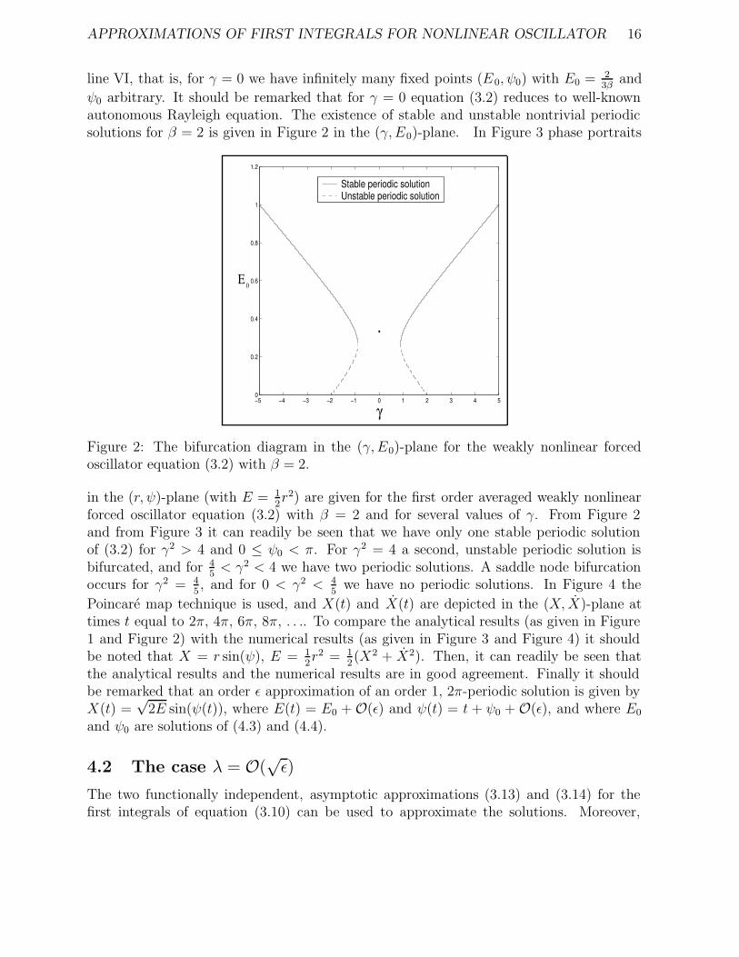
APPROXIMATIONS OF FIRST INTEGRALS FOR NONLINEAR OSCILLATOR 16
line VI, that is, for γ = 0 we have infinitely many fixed points (E0, ψ0) with E0 = 23β
and
ψ0 arbitrary. It should be remarked that for γ = 0 equation (3.2) reduces to well-knownautonomous Rayleigh equation. The existence of stable and unstable nontrivial periodicsolutions for β = 2 is given in Figure 2 in the (γ, E0)-plane. In Figure 3 phase portraits
−5 −4 −3 −2 −1 0 1 2 3 4 50
0.2
0.4
0.6
0.8
1
1.2
γ
Stable periodic solutionUnstable periodic solution
E 0
Figure 2: The bifurcation diagram in the (γ, E0)-plane for the weakly nonlinear forcedoscillator equation (3.2) with β = 2.
in the (r, ψ)-plane (with E = 12r2) are given for the first order averaged weakly nonlinear
forced oscillator equation (3.2) with β = 2 and for several values of γ. From Figure 2and from Figure 3 it can readily be seen that we have only one stable periodic solutionof (3.2) for γ2 > 4 and 0 ≤ ψ0 < π. For γ2 = 4 a second, unstable periodic solution isbifurcated, and for 4
5< γ2 < 4 we have two periodic solutions. A saddle node bifurcation
occurs for γ2 = 45, and for 0 < γ2 < 4
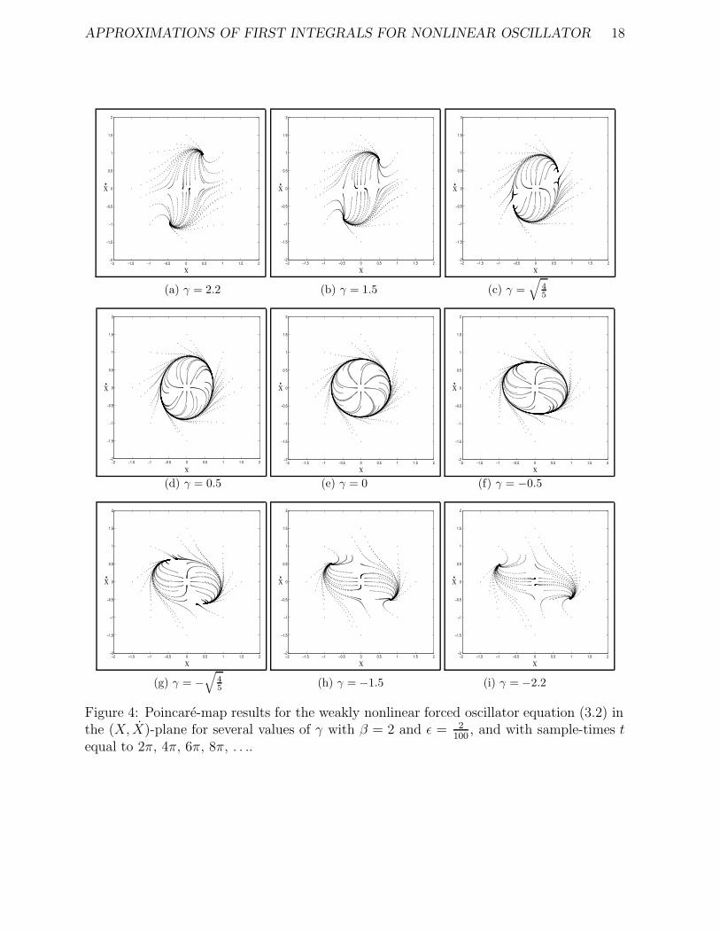
5we have no periodic solutions. In Figure 4 the
Poincare map technique is used, and X(t) and X(t) are depicted in the (X, X)-plane attimes t equal to 2π, 4π, 6π, 8π, . . .. To compare the analytical results (as given in Figure1 and Figure 2) with the numerical results (as given in Figure 3 and Figure 4) it shouldbe noted that X = r sin(ψ), E = 1
2r2 = 1
2(X2 + X2). Then, it can readily be seen that
the analytical results and the numerical results are in good agreement. Finally it shouldbe remarked that an order ε approximation of an order 1, 2π-periodic solution is given byX(t) =
√2E sin(ψ(t)), where E(t) = E0 + O(ε) and ψ(t) = t + ψ0 + O(ε), and where E0
and ψ0 are solutions of (4.3) and (4.4).
4.2 The case λ = O(√ε)
The two functionally independent, asymptotic approximations (3.13) and (3.14) for thefirst integrals of equation (3.10) can be used to approximate the solutions. Moreover,

APPROXIMATIONS OF FIRST INTEGRALS FOR NONLINEAR OSCILLATOR 17
0 0.2 0.4 0.6 0.8 1 1.2 1.4 1.6 1.8 2−3
−2
−1
0
1
2
3
ψ
r0 0.2 0.4 0.6 0.8 1 1.2 1.4 1.6 1.8 2
−3
−2
−1
0
1
2
3
ψ
r0 0.2 0.4 0.6 0.8 1 1.2 1.4 1.6 1.8 2
−3
−2
−1
0
1
2
3
ψ
r
(a) γ = 2.2 (b) γ = 1.5 (c) γ =√
4
5
0 0.2 0.4 0.6 0.8 1 1.2 1.4 1.6 1.8 2−3
−2
−1
0
1
2
3
ψ
r0 0.2 0.4 0.6 0.8 1 1.2 1.4 1.6 1.8 2
−3
−2
−1
0
1
2
3
ψ
r0 0.2 0.4 0.6 0.8 1 1.2 1.4 1.6 1.8 2
−3
−2
−1
0
1
2
3
ψ
r
(d) γ = 0.5 (e) γ = 0 (f) γ = −0.5
0 0.2 0.4 0.6 0.8 1 1.2 1.4 1.6 1.8 2−3
−2
−1
0
1
2
3
ψ
r0 0.2 0.4 0.6 0.8 1 1.2 1.4 1.6 1.8 2
−3
−2
−1
0
1
2
3
ψ
r0 0.2 0.4 0.6 0.8 1 1.2 1.4 1.6 1.8 2
−3
−2
−1
0
1
2
3
ψ
r
(g) γ = −√
4
5(h) γ = −1.5 (i) γ = −2.2
Figure 3: Phase Portraits in the (r, ψ)-plane for the weakly nonlinear forced oscillatorequation (3.2) with β = 2 and for several values of γ.
APPROXIMATIONS OF FIRST INTEGRALS FOR NONLINEAR OSCILLATOR 18
−2 −1.5 −1 −0.5 0 0.5 1 1.5 2−2
−1.5
−1
−0.5
0
0.5
1
1.5
2
X
X
−2 −1.5 −1 −0.5 0 0.5 1 1.5 2−2
−1.5
−1
−0.5
0
0.5
1
1.5
2
X
X
−2 −1.5 −1 −0.5 0 0.5 1 1.5 2−2
−1.5
−1
−0.5
0
0.5
1
1.5
2
X
X
(a) γ = 2.2 (b) γ = 1.5 (c) γ =√
4
5
−2 −1.5 −1 −0.5 0 0.5 1 1.5 2−2
−1.5
−1
−0.5
0
0.5
1
1.5
2
X
X
−2 −1.5 −1 −0.5 0 0.5 1 1.5 2−2
−1.5
−1
−0.5
0
0.5
1
1.5
2
X
X
−2 −1.5 −1 −0.5 0 0.5 1 1.5 2−2
−1.5
−1
−0.5
0
0.5
1
1.5
2
X
X
(d) γ = 0.5 (e) γ = 0 (f) γ = −0.5
−2 −1.5 −1 −0.5 0 0.5 1 1.5 2−2
−1.5
−1
−0.5
0
0.5
1
1.5
2
X
X
−2 −1.5 −1 −0.5 0 0.5 1 1.5 2−2
−1.5
−1
−0.5
0
0.5
1
1.5
2
X
X
−2 −1.5 −1 −0.5 0 0.5 1 1.5 2−2
−1.5
−1
−0.5
0
0.5
1
1.5
2
X
X
(g) γ = −√
4
5(h) γ = −1.5 (i) γ = −2.2
Figure 4: Poincare-map results for the weakly nonlinear forced oscillator equation (3.2) inthe (X, X)-plane for several values of γ with β = 2 and ε = 2
100, and with sample-times t
equal to 2π, 4π, 6π, 8π, . . ..

APPROXIMATIONS OF FIRST INTEGRALS FOR NONLINEAR OSCILLATOR 19
from (3.13) and (3.14) an approximation of a periodic solution (if it exists) can easily beconstructed. Let T < ∞ be the period of a periodic solution (obviously T should be amultiple of π for γ 6= 0). Let G3(E, ψ, t; ε) = constant and G4(E, ψ, t; ε) = constant be twoindependent first integrals, where G3 and G4 are approximated by F3 and F4, respectively,and where F3 and F4 are given by (3.13) and (3.14), respectively. Let c3 and c4 be constantsin the two independent first integrals G3 and G4 respectively for which a periodic solutionexists. Now consider G3 = c3 and G4 = c4 for t = nT and t = (n− 1)T with n ∈ N
+ :
G3 (E(nT ), ψ(nT ), nT ; ε) = c3,
G3 (E ((n− 1)T ) , ψ((n− 1)T ), (n− 1)T ; ε) = c3,
G4 (E(nT ), ψ(nT ), nT ; ε) = c4,
G4 (E ((n− 1)T ) , ψ((n− 1)T ), (n− 1)T ; ε) = c4.
(4.7)
Approximating G3 by F3 and G4 by F4 respectively, eliminating c3 and c4 from (4.7) bysubtractions, and using the transformation ψ(t) = θ(t) +
√ε3
4tE(t), we then obtain
E(nT ) = E ((n− 1)T ) + εT
(
E ((n− 1)T ) − 3
2E ((n− 1)T )2 β
+1
2γE((n− 1)T ) cos(2θ ((n− 1)T ))
)
+ O(ε√εt),
θ(nT ) = θ ((n− 1)T ) − T + εT
(
−105
64E((n− 1)T )2 − 1
4γ sin(2θ ((n− 1)T ))
)
+O(ε√εt), (4.8)
on a time scale of order 1√ε. In fact (4.8) defines a map R : E → R(E) ⇔ En = R(En−1)
which we will use to determine the nontrivial periodic solution(s) of equation (3.10). Byneglecting terms of O(ε
√εt) in (4.8) we can define a new map S : E → S(E) ⇔ En =
S(En−1). It should be remarked that the second equation in the map S (and in the map R)will always be considered modulo T . From the well-known theorem of Hartman-Grobmanit follows that when the map S has a hyperbolic fixed point then the map R also has afixed point which is ε-close to the one of the map S. Moreover, the fixed point of the mapR has the same stability properties as the corresponding fixed point of the map S. In thiscase it follows from (4.8) with γ 6= 0 that the map S has as nontrivial fixed points (E 0, θ0),where E0 is given by
(3βE0 − 2)2 +
(
−105
16E2
0
)2
= γ2, (4.9)
and where θ0 is given by
γ cos(2θ0) = 3E0β − 2 and
γ sin(2θ0) =(
−10516E2
0
)
.
(4.10)

APPROXIMATIONS OF FIRST INTEGRALS FOR NONLINEAR OSCILLATOR 20
The linearized map of map S around a fixed point of map S, is given by
DP =
1 0
0 1
+ εT
1 − 3E0β + 12γ cos(2θ0) −E0γ sin(2θ0)
−10532E0 −1
2γ cos(2θ0)
. (4.11)
By using (4.9) it follows from (4.11) that the eigenvalues of DP are
λ1,2 = 1 + εT
(
1
2− 3
2βE0 ±
1
32
√
256 − 22050E40
)
.
(4.12)
Again if the eigenvalues (4.12) are not equal to one in modules, then the fixed point (E 0, θ0)is hyperbolic. The results as given by (4.9) and (4.10) are exactly the same results as theones which can be obtained by using the second order averaging method or the multipletime-scales method or other perturbation techniques. Using the formulas of Cardano thebifurcation diagram in the (β, γ)-plane can be derived from (4.9) and is given in Figure5. The regions I-V in Figure 5 are as defined in section 4.1. The existence of stable and
β
V
V
VI
IV
IV
III
III
II
II
I
I
γ
Figure 5: The bifurcation diagram in the (β, γ)-plane for the nonlinear map (4.8).
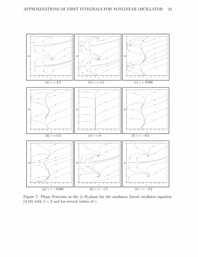
unstable nontrivial equilibrium solutions for the nonlinear map (4.8) with β = 2 can bedetermined from Figure 6 in the (γ, E0)-plane. In Figure 7 the phase portraits in the (r, θ)-plane (with E = 1
2r2) are given for the second order averaged nonlinear forced oscillator
equation (3.10) with β = 2 and for several values of γ. It should be remarked that the fixedpoints as given by (4.9) and (4.10) are not corresponding with the 2π-periodic solutionsof the equation (3.10) due to the transformation θ(t) = ψ(t) − √
ε 34E(t)t. So, the periodic
solutions as given in Figure 5 and 6 for γ 6= 0 are not the 2π-periodic solutions for the
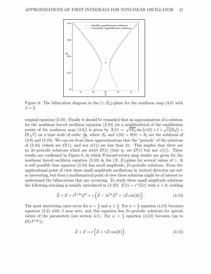
APPROXIMATIONS OF FIRST INTEGRALS FOR NONLINEAR OSCILLATOR 21
E0
γ
: Unstable equilibrium solution: Stable equilibrium solution
Figure 6: The bifurcation diagram in the (γ, E0)-plane for the nonlinear map (4.8) withβ = 2.
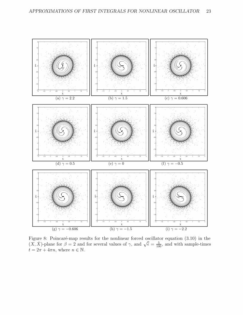
original equation (3.10). Finally it should be remarked that an approximation of a solutionfor the nonlinear forced oscillator equation (3.10) (in a neighborhood of the equilibriumpoints of the nonlinear map (4.8)) is given by X(t) =
√2E0 sin
(
ψ(0) + t +√ε3
4E0t
)
+O(
√ε) on a time scale of order 1√
ε, where E0 and ψ(0) = θ(0) = θ0 are the solutions of
(4.9) and (4.10). We can see from these approximations that the ”periods” of the solutionsof (3.10) (which are O(1), and not o(1)) are less than 2π. This implies that there areno 2π-periodic solutions which are strict O(1) (that is, are O(1) but not o(1)). Theseresults are confirmed in Figure 8, in which Poincare-return map results are given for thenonlinear forced oscillator equation (3.10) in the (X, X)-plane for several values of γ. Itis still possible that equation (3.10) has small amplitude, 2π-periodic solutions. From theapplicational point of view these small amplitude oscillations in vertical direction are notso interesting, but from a mathematical point of view these solutions might be of interest tounderstand the bifurcations that are occurring. To study these small amplitude solutionsthe following rescaling is usually introduced in (3.10): X(t) = εαZ(t) with α > 0, yielding
Z + Z + ε1
2+2αZ3 = ε
(
Z − βε2αZ3 + γZ cos(2t))
. (4.13)
The most interesting cases occur for α = 14
and α > 14. For α = 1
4equation (4.13) becomes
equation (3.2) with β near zero, and this equation has 2π-periodic solutions for specialvalues of the parameters (see section 4.1). For α > 1
4equation (4.13) becomes (up to
O(ε1
2+2α))
Z + Z = ε(
Z + γZ cos(2t))
. (4.14)
APPROXIMATIONS OF FIRST INTEGRALS FOR NONLINEAR OSCILLATOR 22
0 0.2 0.4 0.6 0.8 1 1.2 1.4 1.6 1.8 2−3
−2
−1
0
1
2
3
θ
r0 0.2 0.4 0.6 0.8 1 1.2 1.4 1.6 1.8 2
−3
−2
−1
0
1
2
3
θ
r0 0.2 0.4 0.6 0.8 1 1.2 1.4 1.6 1.8 2
−3
−2
−1
0
1
2
3
θ
r
(a) γ = 2.2 (b) γ = 1.5 (c) γ = 0.606
0 0.2 0.4 0.6 0.8 1 1.2 1.4 1.6 1.8 2−3
−2
−1
0
1
2
3
θ
r0 0.2 0.4 0.6 0.8 1 1.2 1.4 1.6 1.8 2
−3
−2
−1
0
1
2
3
θ
r0 0.2 0.4 0.6 0.8 1 1.2 1.4 1.6 1.8 2
−3
−2
−1
0
1
2
3
θ
r
(d) γ = 0.5 (e) γ = 0 (f) γ = −0.5
0 0.2 0.4 0.6 0.8 1 1.2 1.4 1.6 1.8 2−3
−2
−1
0
1
2
3
θ
r0 0.2 0.4 0.6 0.8 1 1.2 1.4 1.6 1.8 2
−3
−2
−1
0
1
2
3
θ
r0 0.2 0.4 0.6 0.8 1 1.2 1.4 1.6 1.8 2
−3
−2
−1
0
1
2
3
θ
r
(g) γ = −0.606 (h) γ = −1.5 (i) γ = −2.2
Figure 7: Phase Portraits in the (r, θ)-plane for the nonlinear forced oscillator equation(3.10) with β = 2 and for several values of γ.
APPROXIMATIONS OF FIRST INTEGRALS FOR NONLINEAR OSCILLATOR 23
−2 −1.5 −1 −0.5 0 0.5 1 1.5 2−2
−1.5
−1
−0.5
0
0.5
1
1.5
2
X
X
−2 −1.5 −1 −0.5 0 0.5 1 1.5 2−2
−1.5
−1
−0.5
0
0.5
1
1.5
2
X
X
−2 −1.5 −1 −0.5 0 0.5 1 1.5 2−2
−1.5
−1
−0.5
0
0.5
1
1.5
2
X
X
(a) γ = 2.2 (b) γ = 1.5 (c) γ = 0.606
−2 −1.5 −1 −0.5 0 0.5 1 1.5 2−2
−1.5
−1
−0.5
0
0.5
1
1.5
2
X
X
−2 −1.5 −1 −0.5 0 0.5 1 1.5 2−2
−1.5
−1
−0.5
0
0.5
1
1.5
2
X
X
−2 −1.5 −1 −0.5 0 0.5 1 1.5 2−2
−1.5
−1
−0.5
0
0.5
1
1.5
2
X
X
(d) γ = 0.5 (e) γ = 0 (f) γ = −0.5
−2 −1.5 −1 −0.5 0 0.5 1 1.5 2−2
−1.5
−1
−0.5
0
0.5
1
1.5
2
X
X
−2 −1.5 −1 −0.5 0 0.5 1 1.5 2−2
−1.5
−1
−0.5
0
0.5
1
1.5
2
X
X−2 −1.5 −1 −0.5 0 0.5 1 1.5 2
−2
−1.5
−1
−0.5
0
0.5
1
1.5
2
X
X
(g) γ = −0.606 (h) γ = −1.5 (i) γ = −2.2
Figure 8: Poincare-map results for the nonlinear forced oscillator equation (3.10) in the(X, X)-plane for β = 2 and for several values of γ, and
√ε = 5
100, and with sample-times
t = 2π + 4πn, where n ∈ N .
APPROXIMATIONS OF FIRST INTEGRALS FOR NONLINEAR OSCILLATOR 24
In the Appendix 1 (4.14) is studied briefly. From the Poincare expansion theorem it followsthat all solutions of (3.10) can be expand in X0(t)+
√εX1(t)+εX2(t)+. . . on a time-scale of
order 1. Obviously X0 +X0 = 0. So, from the Poincare expansion theorem and the resultsobtained in this section it follows that equation (3.10) can only have small amplitude,2π-periodic solutions as periodic solutions.
4.3 The case λ = O(1)
The two functionally independent, asymptotic approximation (3.21) and (3.22) for the firstintegrals of equation (3.18) can be used to determine the existence of the time-periodicsolutions. Moreover, from (3.21) and (3.22) an approximation of a periodic solution caneasily be constructed. Let T <∞ be the period of a periodic solution (obviously T shouldbe πl, with l ∈ N
+ for γ 6= 0). Let G5(E, ψ, t; ε) = constant and G6(E, ψ, t; ε) = constant
be two independent first integrals, where G5 and G6 are approximated by F5 and F6,respectively, and where F5 and F6 are given by (3.21) and (3.22), respectively. Let c5 andc6 be constants in the two independent first integrals for which a periodic solution exists.Now consider G5 = c5 and G6 = c6 for t = 0 and t = T . Approximating G5 by F5 andG6 by F6 (as given by (3.21) and (3.22)), eliminating c5 and c6 by subtractions, we thenobtain (using the fact that E(0) = E(T ) for a periodic solution)
ε∫ T
0
(
X2 − βX4 + γX2 cos(2s))
ds = O(ε2),
ε∫ T
0P1(ϑ, k)
(
X − βX3 + γX cos(2s))
ds = O(ε2),
(4.15)
where X = −ω0A0sn(ϑ, k)dn(ϑ, k). We can rewrite equation (4.15) as
εI(E, ψ, β, γ) = O(ε2),
εJ(E, ψ, β, γ) = O(ε2).(4.16)
To have a periodic solution for (3.18) we have to find an energy E and a phase angle ψsuch that I(E, ψ, β, γ) and J(E, ψ, β, γ) are equal to zero (see also [12, 14]). To find thisenergy and phase angle we rewrite I(E, ψ, β, γ) and J(E, ψ, β, γ) in
I ≡ I1 − βI2 + γI3 = 0,
J ≡ J1 − βJ2 + γJ3 = 0,(4.17)
where
I1 =∫ T
0X2ds, I2 =
∫ T
0X4ds, I3 =
∫ T
0
(
X2 cos(2s))
ds,
J1 =∫ T
0P1(ϑ, k)Xds, J2 =
∫ T
0P1(ϑ, k)X
3ds, J3 =∫ T
0P1(ϑ, k)
(
X cos(2s))
ds.
(4.18)

APPROXIMATIONS OF FIRST INTEGRALS FOR NONLINEAR OSCILLATOR 25
Let D = I3J2 − I2J3. It follows from (4.17) that for a periodic solution to exist β and γ,can be considered to be functions of the energy E and the phase angle ψ, that is,
β = 1D
(I3J1 − I1J3) ,
γ = 1D
(I2J1 − I1J2) ,(4.19)
for D 6= 0. By using an adaptive recursive Simpson rule the values of the parameters β andγ can be calculated from (4.17)-(4.19) for which a periodic solution exists. From (3.18) itis obvious that the period T should be a multiple of π. The expansion theorem of Poincareimplies that the solution(s) of (3.18) can be expanded in X0(t)+εX1(t)+ε2X2(t)+ . . . on atime-scale of order 1, where X0 satisfies X0+X0+X3
0 = 0. Now X0(t) is a periodic function
with period T0(E0) = 4∫ A0
01√
2E0−X2
0− 1
2X4
0
dX0, where A0 > 0 satisfies 2E0 −A20 − 1
2A4
0 = 0.
In Figure 9 T0(E0) is plotted. From Figure 9 and from the fact that T should be a multiple
2.6
2.8
3
3.2
3.4
3.6
3.8
4
4.2
4.4
4.6
4.8
5
5.2
5.4
5.6
5.8
6
6.2
0 2 4 6 8 10 12 14 E0
π
T0
π2
Figure 9: The period T0 of the unperturbed equation (3.18) (that is, (3.18) with ε = 0) asfunction of the energy E0 = 1
2X2
0 + 12X2
0 + 14X4
0 .
of π it immediately follows that T should be equal to π or 2π. For 2π-periodic solutionsit follows from Figure 9 that E0 should be zero, and so a 2π-periodic solution (if it exists)should have a small amplitude. To study these small amplitude solutions the followingrescaling is introduced in (3.18): X(t) = εαZ(t) with α > 0, yielding
Z + Z = −ε2αZ3 + εZ − ε1+2αβZ3 + εγZ cos(2t). (4.20)
For 2π-periodic solutions Z(t) only the case α = 12
and the case α > 12
have to be considered.For α = 1
2equation (4.20) becomes equation (3.2) with β near zero, and this equation has
APPROXIMATIONS OF FIRST INTEGRALS FOR NONLINEAR OSCILLATOR 26
2π-periodic solutions for special values of the parameters (see section 4.1). For α > 12
equation (4.14) up to O(ε2α) is again obtained, and this equation has been studied brieflyin Appendix 1. For π-periodic solutions it follows from Figure 9 that E 0 should be near6.33552259..., and so a π-periodic solution (if it exists) should have an amplitude of (strict)O(1). To determine the values of β and γ for which a π-periodic solution exists it shouldbe observed that β = β(E0, ψ0) and γ = γ(E0, ψ0), where E0 = 6.33552259... and 0 ≤ ψ0 ≤4K(k) (in which K(k) is the complete elliptic integral of the first kind). For different valuesof ψ0 (with E0 = 6.33552259...) the integrals in (4.18) and (4.19) have been calculated byusing an adaptive recursive Simpson rule. It should be observed that in (4.18)X(t) (that is,the solution of the unperturbed equation (3.18) with ε = 0) depends on the initial energy E 0
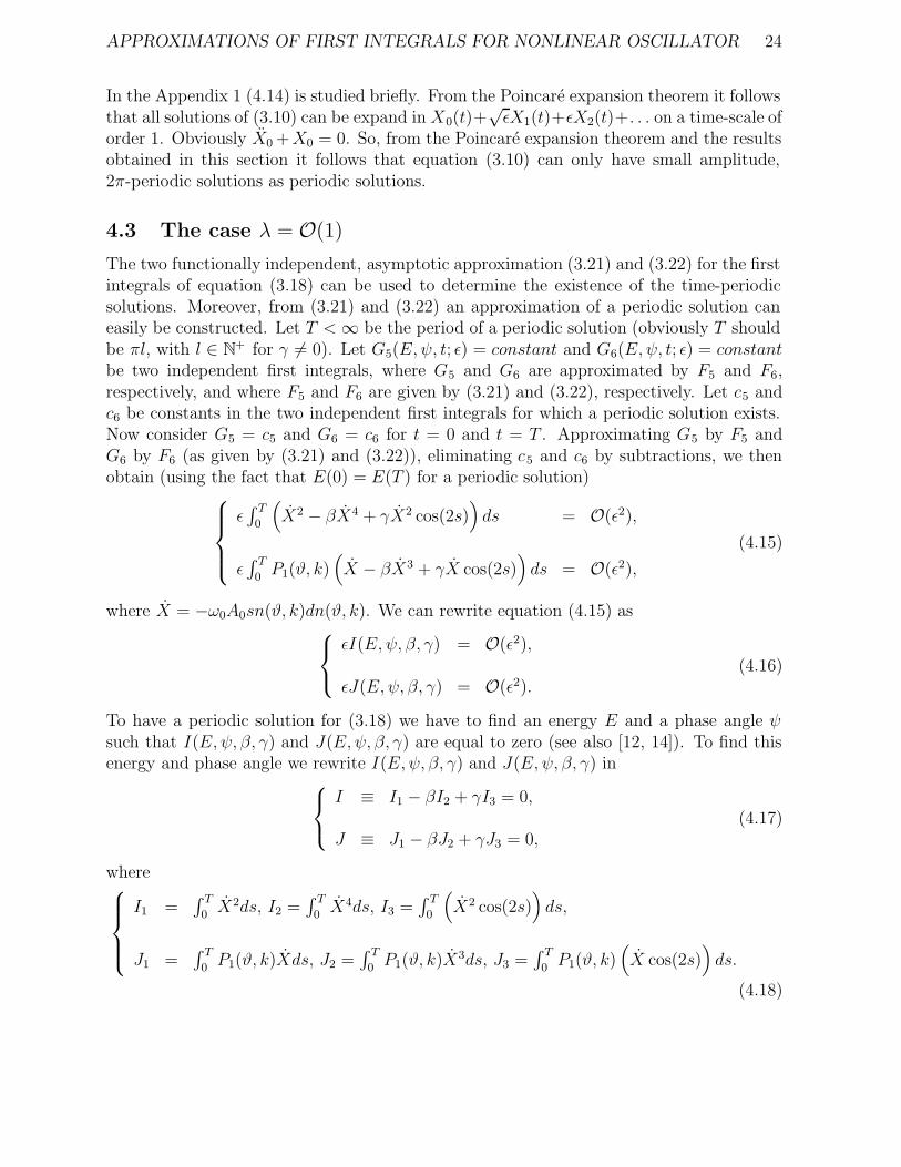
and on the initial phase angle ψ0. For E0 = 6.33552259... β = β(E0, ψ0) and γ = γ(E0, ψ0)will give a curve in the (β, γ)-plane. This curve has been determined numerically, and isgiven in Figure 10. From a practical point of view it is obvious that the chance that the
–0.4
–0.2
0
0.2
0.4
0.084 0.088 0.092 0.096
γ
β
Figure 10: The curve in the (β, γ)-plane for which the strongly nonlinear forced equation(3.18) has π-periodic solutions of order 1.
parameters β and γ are on this curve is of course zero. For that reason also Poincare-mapresults are given in Figure 11 for different values of β and γ.
5 Conclusions and remarks
In this paper it has been shown that the perturbation method based on integrating factorscan be used efficiently to approximate first integrals for strongly nonlinear forced oscillators.In section 2 (and 3) of this paper a justification of the presented perturbation method hasbeen given. It has also been shown how the existence and stability of time-periodic solutions

APPROXIMATIONS OF FIRST INTEGRALS FOR NONLINEAR OSCILLATOR 27
−1 −0.8 −0.6 −0.4 −0.2 0 0.2 0.4 0.6 0.8 1−1
−0.8
−0.6
−0.4
−0.2
0
0.2
0.4
0.6
0.8
1
X
X−0.4 −0.2 0 0.2 0.4
−0.4
−0.2
0
0.2
0.4
X
X−1 −0.8 −0.6 −0.4 −0.2 0 0.2 0.4 0.6 0.8 1
−1
−0.8
−0.6
−0.4
−0.2
0
0.2
0.4
0.6
0.8
1
X
X
(a) γ = 2.2 (b) Zoom in for γ = 2.2 (c) γ = 1.5
−0.4 −0.2 0 0.2 0.4−0.4
−0.2
0
0.2
0.4
X
X−1 −0.8 −0.6 −0.4 −0.2 0 0.2 0.4 0.6 0.8 1
−1
−0.8
−0.6
−0.4
−0.2
0
0.2
0.4
0.6
0.8
1
X
X−1 −0.8 −0.6 −0.4 −0.2 0 0.2 0.4 0.6 0.8 1
−1
−0.8
−0.6
−0.4
−0.2
0
0.2
0.4
0.6
0.8
1
X
X
(d) Zoom in for γ = 1.5 (e) γ = 0 (f) γ = −1.5
−0.4 −0.2 0 0.2 0.4−0.4
−0.2
0
0.2
0.4
X
X−1 −0.8 −0.6 −0.4 −0.2 0 0.2 0.4 0.6 0.8 1
−1
−0.8
−0.6
−0.4
−0.2
0
0.2
0.4
0.6
0.8
1
X
X−0.4 −0.2 0 0.2 0.4
−0.4
−0.2
0
0.2
0.4
X
X
(g) Zoom in for γ = −1.5 (h) γ = −2.2 (i) Zoom in for γ = −2.2
Figure 11: Poincare-map results for the nonlinear forced oscillator equation (3.18) in the(X, X)-plane for several values of γ with β = 2 and ε = 2
100, and with sample-times t = πn
with n ∈ Z+ for the figures (a), (c), (e), (f), and (h), and t = −2πn with n ∈ Z
+ for thefigures (b), (d), (g), and (i).

APPROXIMATIONS OF FIRST INTEGRALS FOR NONLINEAR OSCILLATOR 28
can be deduced from the approximations of the first integrals for the strongly nonlinearforced oscillators.In this paper the following three oscillator equations have been studied in detail:
X +X = ε(
X − βX3 −X3 + γX cos(2t))
, (5.1)
X +X +√εX3 = ε
(
X − βX3 + γX cos(2t))
, and (5.2)
X +X +X3 = ε(
X − βX3 + γX cos(2t))
, (5.3)
where ε is a small parameter with 0 < ε � 1, and where β > 0 and γ 6= 0 are constants(of order 1). In particular the O(1) behavior of the solutions has been studied. Fromthe applicational point of view this O(1)-behavior is the most interesting behavior whengalloping is studied. For equation (5.1) it has been shown for what values of the parametersthe solutions will tend to a 2π-periodic solution of order 1, and for what values of theparameters the solutions will tend to a (non-periodic) bounded attractor. The resultsobtained for (5.1) are in agreement with the results as obtained in [2, 3]. For equation(5.2) it has been shown that there are no periodic solutions of order 1. Small amplitude,2π-periodic solutions, however, exist for certain values of the parameters. In general thesolutions will tend to a bounded, non-periodic attractor of order 1. For equation (5.3) it hasbeen shown that there are π-periodic solutions of order 1 for special values of parameters.These π-periodic solutions are, however, structurally unstable. Also small amplitude, 2π-periodic solutions exist for certain values of parameters. In general the solutions will tendto a bounded, non-periodic attractor of order 1.
A Appendix 1
In section 4.2 and in section 4.3 the following ODEs have been derived to describe thesmall amplitude solutions of the oscillator equations
Z + Z = ε(
Z + γZ cos(2t))
− ε1
2+2αZ3 − ε1+2αβZ3, and (1.4)
Z + Z = ε(
Z + γZ cos(2t))
− ε2αZ3 − ε1+2αβZ3, (1.5)
with α > 14
and with α > 12
respectively. In this appendix (1.4) and (1.5) will be studiedbriefly. By introducing the transformation
Y (t) = Y1(t) cos(t) + Y2(t) sin(t),
Y (t) = −Y1(t) sin(t) + Y2(t) cos(t),(1.6)
the first order averaged system of equation (1.4) or of equation (1.5) becomes
Y1 = ε(
12Y1 − 1
4γY1
)
,
Y2 = ε(
14γY2 + 1
2Y2
)
.
(1.7)
APPROXIMATIONS OF FIRST INTEGRALS FOR NONLINEAR OSCILLATOR 29
For γ2 not in an o(1) neighborhood of 4 system (1.7) has only as fixed point(s) the trivialfixed point (0, 0). This fixed point turns out to be unstable. So, for γ 2 not in an o(1) neigh-borhood of 4 it can be conclude that (1.4) and (1.5) do not have nontrivial, 2π-periodicsolutions. For γ2 in an o(1) neighborhood of 4 second order or higher order averaginghas to be applied to (1.4) or (1.5). Again it can be shown that (1.4) and (1.5) do nothave nontrivial, 2π-periodic solutions. The elementary calculations to prove this will beomitted.
Acknowledgment–This research project was sponsored by the Secondary Teacher Development Pro-
gramme (PGSM)(Indonesia) and The University of Technology in Delft (The Netherlands).
References
[1] A.H. Nayfeh and D.T. Mook, Nonlinear Oscillations, John Wiley & Sons, New York,1985.
[2] C.G.A. van der Beek, Normal form and periodic solutions in the theory of non-linearoscillations. Existence and asymptotic theory, International journal of non-linear me-
chanics,Vol. 24, No. 4, 1989, pp. 263-279.
[3] C.G.A. van der Beek, Analysis of a system of two weakly nonlinear coupled harmonicoscillators arising from the field of wind-induced vibrations, International journal of
non-linear mechanics,Vol. 27, No. 4, 1992, pp. 679-704.
[4] D.F. Lawden, Elliptic Functions and Applications, Springer-Verlag, New York, 1989.
[5] J.D. Brothers and R. Haberman, Accurate Phase after Passage through SubharmonicResonance, SIAM J.Appl. Math., Vol. 59, No. 1, 1998, pp. 347-364.
[6] K. Yagasaki and T. Ichikawa, Higher-Order Averaging for Periodically Forced, WeaklyNonlinear Systems, Int.J. of Bifurcation and Chaos 9(3), 1999, pp. 519-531.
[7] K. Yagasaki, Melnikov’s Method and Codimension-Two Bifurcations in Forced Oscil-lations, Journal of Differential Equations 185, 2002, pp. 1-24.
[8] M. Belhaq and M. Houssni, Quasi-Periodic Oscillations, Chaos and Suppression ofChaos in a Nonlinear Oscillator Driven by Parametric and External Excitations, Non-
linear Dynamics 18, 1999, pp. 1-24.
[9] P.F. Byrd and M.D. Friedman, Handbook of Elliptic Integrals for Engineers and Sci-
entists, 2nd, Berlin Springer, Berlin,1971.
[10] R. Lima and M. Pettini, Suppression of chaos by resonance parametric perturbations,Physical Review A 41, 1990, pp. 726-733.

APPROXIMATIONS OF FIRST INTEGRALS FOR NONLINEAR OSCILLATOR 30
[11] R.V. Roy, Averaging Methods for strongly Non-linear Oscillators with Periodic Exci-tations, Int.J. Non-linear Mechanics, Vol.29 No 5, 1994, pp. 737-753.
[12] S.B. Waluya and W.T. van Horssen, Asymptotic Approximations of First Integralsfor a Nonlinear Oscillator, Nonlinear Analysis, Vol.51 No 8, 2002, pp. 1327-1346.
[13] S.B. Waluya and W.T. van Horssen, On Approximations of First Integrals for a Systemof Weakly Nonlinear, Coupled Harmonic Oscillators, Nonlinear Dynamics 30, 2002,pp. 243-266.
[14] S.B. Waluya and W.T. van Horssen, On Approximations of First Integrals for StronglyNonlinear Oscillators, to be published in Nonlinear Dynamics.
[15] S.H. Chen and Y.K. Cheung, An Elliptic Lindstedt-Poincare for certain strongly Non-linear Oscillators, Nonlinear Dynamics 12, 1997, pp. 199-213.
[16] S.H. Chen and Y.K. Cheung, An Elliptic Perturbation Method for certain stronglyNon-linear Oscillators, Journal of Sound and Vibration 192(2), 1996, pp. 453-464.
[17] T.D. Burton and Z. Rahman, On Multiple-Scale Analysis of Strongly Non-LinearForced Oscillators, Int.J. Non-linear Mechanics, Vol.21 No 2, 1986, pp. 135-146.
[18] T.I. Haaker and A.H.P. van der Burgh, Rotational Galloping of Two Coupled Oscil-lators, Mechanica 33, 1998, pp. 219-227.
[19] V.T. Coppola and R.H. Rand, Averaging using Elliptic Functions:approximation oflimit cycles, Acta Mechanica 81, 1990, pp. 125-142.
[20] W.T. van Horssen, A Perturbation Method Based on Integrating Factors, SIAM jour-
nal on Applied Mathematics, Vol. 59, No. 4, 1999, pp. 1427-1443.
[21] W.T. van Horssen, A Perturbation Method Based on Integrating Vectors and MultipleScales, SIAM journal on Applied Mathematics, Vol. 59, No. 4, 1999, pp. 1444-1467.