Deliverable-3.2

Initial specification and proof of conceptimplementation of techniques to enhance

performance and resource utilization in networksDeliverable Editor: Michael Welzl, UiO

Publication date: 30-April-2015Deliverable Nature: Report/SoftwareDissemination level(Confidentiality):

PU (Public)

Project acronym: PRISTINEProject full title: PRogrammability In RINA for European Supremacy of

virTualIsed NEtworksWebsite: www.ict-pristine.euKeywords: ACC, qos-aware multi-path routing, C/U multiplexing,

topological addressing, multi-layer routingSynopsis: This document describes the theoretical analysis,

simulation and initial PoC implementation of resource-utilization and performance enhancing techniques; whichaddress the main requirements described in D3.1.

The research leading to these results has received funding from the European Community's Seventh FrameworkProgramme for research, technological development and demonstration under Grant Agreement No. 619305.

Ref. Ares(2015)3645348 - 04/09/2015

Deliverable-3.2

2

Copyright © 2014-2016 PRISTINE consortium, (Waterford Institute of Technology, Fundacio Privadai2CAT - Internet i Innovacio Digital a Catalunya, Telefonica Investigacion y Desarrollo SA, L.M.Ericsson Ltd., Nextworks s.r.l., Thales Research and Technology UK Limited, Nexedi S.A., BerlinInstitute for Software Defined Networking GmbH, ATOS Spain S.A., Juniper Networks Ireland Limited,Universitetet i Oslo, Vysoke ucenu technicke v Brne, Institut Mines-Telecom, Center for Research andTelecommunication Experimentation for Networked Communities, iMinds VZW.)

List of Contributors

Deliverable Editor: Michael Welzl, UiOi2cat: Francisco Miguel Tarzan Lorente, Leonardo Bergesio, Eduard Grasaimt: Fatma Hriziatos: Miguel Angeluio: Peyman Teymoori, Michael Welzlcn: Roberto Riggio, Kewin Rauschupc: Sergio Leon Gaixas, Jordi Perellotssg: Micheal Crottyexternal: John Day

Disclaimer

This document contains material, which is the copyright of certain PRISTINEconsortium parties, and may not be reproduced or copied without permission.

The commercial use of any information contained in this document may require alicense from the proprietor of that information.

Neither the PRISTINE consortium as a whole, nor a certain party of the PRISTINEconsortium warrant that the information contained in this document is capable ofuse, or that use of the information is free from risk, and accept no liability for loss ordamage suffered by any person using this information.

Deliverable-3.2

3

Executive SummaryIn this document, "an initial specification and a proof of concept implementation" ofthe techniques proposed in the previous document, "draft specification", are presented.The goal is to show how the proposed techniques in the previous document can beimplemented in RINA as a proof of concept, what their performance improvement isover other similar methods (if applicable), and what future directions are. The activitiesperformed in D3.2 are centered around three main areas of i) programmable congestioncontrol; ii) unification of connection-oriented and connectionless resource allocationin support of multiple levels of service; and iii) topological addressing to bound routingtable sizes. This document also specifies the investigation results of these techniquesas some initial policies in RINA.

In the first chapter, programmable congestion control, we will specify some newpolicies on how to implement a simple congestion control mechanism behaving likeTCP. Then we will enhance it with an aggregate pushback mechanism. To compareit with other similar methods, we implemented Split-TCP, which is the most similarmethod in the Internet to our implementation in RINA. We show that RINA’scongestion control performs similar to Split-TCP, and both outperform TCP. Thesecond part of chapter one discusses a practical use-case of the application of RINA’sprogrammable congestion control policies for the DC use case. Specific congestiondetection and mitigation policies are proposed for the isolation of multiple tenant DIFssharing the resources provided by the DC-Fabric DIF.

In chapter 2, two aspects of resource allocation in a DIF are explored: multiplexing andexploiting multiple equal-cost paths. The first part of chapter 2 discusses the Cherish/Urgency multiplexing scheme, by which it is possible to provide strict differentialdelay and loss guarantees to different flows provided by a DIF. We first present thismultiplexing approach in the context of the more general ΔQ framework. Next weanalyze how this multiplexing approach can be decomposed into the different RMTpolicies, propose a specification for those policies and perform an initial performanceevaluation using RINAsim. The second part of the chapter is dedicated to exploring aQoS-aware multi-path routing approach in the context of the datacentre networkinguse case. The fact that a DIF is aware of the QoS requirements of the flows providedto the applications using the DIF opens the door to more effective and dynamic multi-path strategies than the traditional Equal Cost Multi Path (ECMP) approach.

In chapter 3, Topological Addressing to Bound Routing Table Sizes, we presentnew generic architectures for routing and addressing tailored to cope with the

Deliverable-3.2

4

different PRISTINE use cases requirements in terms of scalability, reliability andefficiency. Moreover, these architectures are designed to benefit from RINA’s recursivearchitecture. A couple of routing policies have been implemented and tested along withthe proposed architectures in order to examine the performance of applying RINA tothe use cases, specifically the distributed clouds use case. Simulation results show thata significant improvement of the routing table size is achieved.

Deliverable-3.2

5

Table of Contents1. Congestion control .................................................................................................... 6

1.1. Programmable Congestion Control ................................................................ 61.2. Policies for performance isolation in multi-tenant data centres .................. 16

2. Resource Allocation ................................................................................................ 242.1. Traffic differentiation via delay-loss multiplexing policies .......................... 242.2. QoS-aware Multipath Routing ..................................................................... 38

3. Topological addressing to bound routing table sizes ............................................. 573.1. Introduction .................................................................................................. 573.2. Routing and Addressing in PRISTINE Use Cases ....................................... 573.3. Conclusion .................................................................................................... 78

List of acronyms ......................................................................................................... 80References ................................................................................................................... 83

Deliverable-3.2

6

1. Congestion control

1.1. Programmable Congestion Control

1.1.1. Introduction

Congestion control is done by the TCP protocol in the Internet in an "end-to-end"fashion. The sender is responsible of recovering lost packets, guessing the right sendingrate, and avoiding from congesting the network. This ends up in problems such asignorance of the underlying technology and lengthening the time-to-notify of thesender, which result in losing efficiency. RINA, with its strong layering, allows to attainefficiency in a divide-and-conquer manner, which enables usage of more elaboratemechanisms inside the network wherever they do fit.

We specify how congestion control has been implemented in RINA. By the recursivenature of RINA, its congestion control is bound to one DIF, making a series of DIFsoperate in a fashion that is similar to split-TCP (in case the per-DIF congestion controlpolicy is TCP-like). First we introduce RINA congestion control policies, and then, wepresent simulation results compared with TCP and Split-TCP [SplitTCP].

1.1.2. RINA ACC Policies

Here, we specify the policies implemented/used for ACC in RINA. A simple DIF inshown in Figure 1, “A simple DIF” in which there are a sender, a relay, and a receiverIPC processes.

Figure 1. A simple DIF

1.1.2.1. RMT Policies

• RMTQMonitorPolicy: This policy can be invoked whenever a PDU is placed in aqueue and may keep additional variables that may be of use to the decision processof the RMTSchedulingPolicy and/or RMTMaxQPolicy. Policy implementations:

Deliverable-3.2

7

◦ REDMonitor: Using this implementation, the average queue length is calculatedand passed to REDDropper.

• RMTMAXQPolicy: This policy is invoked when a queue reaches its threshold orexceeds its maximum queue length allowed for this queue. Policy implementations:

◦ ECNMarker: Using this implementation, if the queue length is exceeding itsmaximum threshold, RMT marks the current PDU by setting its ECN bit.

◦ REDDropper: Using this implementation, if the queue length is exceeding itsthreshold, RMT drops the packet with a probability proportional to the amountexceeding the threshold.

◦ UpstreamNotifier: Using this implementation, if the output queue size of RMTexceeds a maximum threshold when inserting a new PDU to an output queue,the RMT requests the Resource Allocator (RA) to send a direct congestionnotification to the sender of that PDU using a CDAP message.

◦ REDUpstreamNotifier: By this implementation, if the queue size of RMTexceeds the initial threshold when inserting a new PDU to the queue but it isshorter than the max threshold, RMT requests the Resource Allocator (RA) tosend a direct congestion notification to the sender of that PDU using a CDAPmessage with a probability proportional to the amount exceeding the initialthreshold.

1.1.2.2. EFCP Policies

• DTCPTxControlPolicy: This policy is used when there are conditions thatwarrant sending fewer PDUs than allowed by the sliding window flow control, e.g.the ECN bit is set in a control PDU. Policy implementations:

◦ DTCPTxControlPolicyTCPTahoe: This is a TCP-like congestion controlimplementation in RINA. The pseudo code of this policy is shown in Algorithm1. Procedure Initialize sets initial values of the local variables. In Send, if thereis credit for transmission, it sends as many PDUs as allowed by the minimumof its send credit and the flow control window, and then, it adjusts its variables.If there is no credit remaining, it closes the DTCP window. In case of receivingacknowledgment packets, it adjusts cwnd and the other variables. If on anydownstream link congestion happens, it receives a notification in the forms ofdirect CDAP messages (via the Resource Allocator), duplicate acknowledgment,or timeout. In the latter case, it starts from slow start, and in the former cases, ithalves its cwnd and goes to congestion avoidance.

Deliverable-3.2

8

◦ DTCPTxControlPolicyTCPWireless: This implementation is used for the DIFsfunctioning over a wireless link where a packet loss does not always implycongestion.

• DTPRTTEstimatorPolicy: This policy is used to calculate Round-Trip-Time(RTT). Policy implementations:

◦ DTPRTTEstimatorPolicyTCP: To calculate RTT and Retransmission Timeout(RTO) for DTCPTxControlPolicyTCPTahoe, this policy is run every time anacknowledgment is received. The pseudo code of this policy is shown inAlgorithm 2.

• DTCPSenderAckPolicy: This policy is triggered when a sender receives anacknowledgment. Policy implementations:

◦ DTCPSenderAckPolicyTCP: This policy performs the default bahavior of RINAupon receiving ACKs, and further it counts the number of PDUs acknowledged.Then, it calls OnRcvACKs of DTCPTxControlPolicyTCPTahoe.

• DTCPECNPolicy: This policy is invoked upon receiving a PDU with ECN bit setin its header.

• ECNSlowDownPolicy: This policy is triggered when an explicit congestionnotification is sent by the Resource Allocator of a congested relay node to the IPCProcess of the sending EFCP of a PDU. Clearly, both IPC Processes are in thesame DIF. The notification is sent as a CDAP message. In other words, this is thecorresponding policy triggered by UpstreamNotifier in the sending EFCP. Policyimplementations:

◦ TCPECNSlowDownPolicy: Referring to Algorithm 1, this policy only calls theOnRcvSlowDown procedure of DTCPTxControlPolicyTCPTahoe in case of usingDTCPTxControlPolicyTCPTahoe as DTCPTxControlPolicy.

Deliverable-3.2

9

Figure 2. Algorithm 1

Deliverable-3.2

10

Figure 3. Algorithm 2

1.1.3. Discussion on the Use of ACC Policies

It should be noted that different combinations of the above policies can be used ina network. Furthermore, different layers might use different kinds of policies, or thepolices are chained among layers to create a chained pushback up to the root cause ofcongestion. A sample general architecture of N layers is illustrated in Figure 4, “Layeredupstream notification in RINA”. The dashed, curved arrows in the figure representnotification transmission between modules. Assume that we only use UpstreamNotifierin the RMTs in the network. In case of congestion in 1-DIF, the Resource Allocator(RA) of the transmitting IPC Process sends a notification to the IPC Process of theEFCP instance sending the PDU, the EFCP instance is located in the same IPC process.The congestion might end up in the closed window queue length growth in the EFCPinstance. If the closed window queue length reaches its maximum size limit, the EFCPshuts down it incoming port, and PDUs are backlogged in the upper RMT output queue.The port is unblocked if the queue length decreases. The output queue of the RMT in 2-DIF might reach its maximum threshold. Since this RMT also uses UpstreamNotifier,this process continues; it sends a slow down signal to the RA and the RA sends anotification to the sending EFCP instance. This pushback notification continues until itreaches the source of congestion. It is worth noting that the EFCP instance transmittingthe traffic at each layer might be carrying the traffic of an aggregate of upper-layer

Deliverable-3.2

11

flows which have been mapped to one lower-layer flow. This is why we call it AggregateCongestion Control (ACC).

The combination of the above policies can facilitate handling of some complicatedsituations. For example, in a wireless link, a packet loss may not be a sign ofcongestion, but a backlogged output queue over time is. By considering this fact,a DTCPTxControlPolicy policy such as DTCPTxControlPolicyTCPWireless describedabove can be developed that halves its cwnd only when it receives a notification from anUpstreamNotifier policy; if it receives, for example, triple duplicate acknowledgments,it does not halves its cwnd as the normal TCP does.

Since sending a direct notification to the sending EFCP instance might affect scalability,especially when the upstream path towards the sender/s is loaded. This depends onthe network topology and the usage scenario. In this case, other policies such asREDUpstreamNotifier, ECNMarker, or REDDropper should be used.

Figure 4. Layered upstream notification in RINA

1.1.4. Evaluation: Simple ACC

RINA has been implemented in the state-of-the-art discrete event simulation toolOMNet. This implementation provide a varieties of policies with default behavior whichcan be customized or extended for developing new protocols and applications. In thissection, we present simulation results of ACC in RINA compared with TCP and Split-TCP. We implemented Split-TCP in the INET framework of OMNet.

1.1.4.1. Comparison of RINA-ACC with TCP and Split-TCP

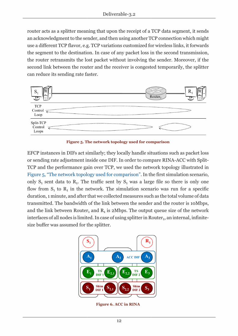
The simplest topology for using Split-TCP is shown in Figure 5, “The network topologyused for comparison”; there is a router in the path from sender S1 to receiver R1. This

Deliverable-3.2

12

router acts as a splitter meaning that upon the receipt of a TCP data segment, it sendsan acknowledgment to the sender, and then using another TCP connection which mightuse a different TCP flavor, e.g. TCP variations customized for wireless links, it forwardsthe segment to the destination. In case of any packet loss in the second transmission,the router retransmits the lost packet without involving the sender. Moreover, if thesecond link between the router and the receiver is congested temporarily, the splittercan reduce its sending rate faster.

Figure 5. The network topology used for comparison

EFCP instances in DIFs act similarly; they locally handle situations such as packet lossor sending rate adjustment inside one DIF. In order to compare RINA-ACC with Split-TCP and the performance gain over TCP, we used the network topology illustrated inFigure 5, “The network topology used for comparison”. In the first simulation scenario,only S1 sent data to R1. The traffic sent by S1 was a large file so there is only oneflow from S1 to R1 in the network. The simulation scenario was run for a specificduration, 1 minute, and after that we collected measures such as the total volume of datatransmitted. The bandwidth of the link between the sender and the router is 10Mbps,and the link between Router1 and R1 is 2Mbps. The output queue size of the networkinterfaces of all nodes is limited. In case of using splitter in Router1, an internal, infinite-size buffer was assumed for the splitter.

Figure 6. ACC in RINA

Deliverable-3.2

13

In case of using RINA-ACC whose architectural view is also shown in Figure 6, “ACC inRINA”, DTCPTxControlPolicyTCPTahoe was activated for both EFCPs in IPC processesE2,2 and A1. In addition, the UpstreamNotifier policy was set for the RMTs in IPCprocesses E2,2 and A2. This configuration of pushback means that if congestion happensbetween the router and the receiver, first the RMT in E2,2 detects it through observingits output queue length by UpstreamNotifier; if the queue length exceeds its initialthreshold, the RMT sends a pushback notification to the sender of the last PDU pushedinto that queue. Since E2,2 is in the TS DIF 2, the sender is the EFCP inside E2,2 whichreceives the pushback notification and slows down. If there are other SDUs waitingfor this EFCP to be transmitted and the congestion window does not allow it, they arebacklogged in the closed window queue of the EFCP. If the relayed PDUs in A2 havea higher rate, then the closed window queue length of the EFCP in E2,2 is built up;upon reaching its maximum limit, the EFCP stops receiving more SDUs from the upperRMT in A2. In particular, EFCP shuts down its incoming port until the closed windowqueue has empty space which as a result, unblocks the port. If the relay rate of A2 is stillhigh, the length of its output queue towards E2,2 grows until it reaches its maximumthreshold. Since this RMT uses UpstreamNotifier too, in this situation, it sends a directCDAP notification to the EFCP instance of the sender of the last PDU pushed into thequeue. At this layer, the notification receiver is the EFCP instance of A1 which is locatedin the sender node.

In case of using TCP, since the second link is slower and it is going to be saturatedsoon which results in packet drop in the output link of the router towards thereceiver, the sender will be notified implicitly by receiving duplicate acknowledgments.The TCP flavor used in the TCP and Split-TCP cases was TCPReno with SelectiveAcknowledgment (SACK) enabled.

Figure 7, “Congestion window size” shows the congestion window size of RINA-ACC,Split-TCP, and TCP for the above scenario where the link delay between the senderand the router is 75ms, and 25ms between the router and the receiver which resultin a total Round-Trip-Time (RTT) of 200ms without any queuing delay. We see thatcwnd of TCP increases until it receives a decrement notification. Due to the longer time-to-notify duration, it increases to much higher or lower values of the optimum rate atwhich it should be sending. Instead, RINA-ACC and Split-TCP, RINA-ACC:Relay andSplit-TCP:Splitter in the figure, react faster to such notifications. Since the link wasslow during the whole simulation time, the sender had to reduce its rate. We can seethat cwnd of RINA-ACC:Sender decreases as well at two time instants.

Deliverable-3.2

14

Figure 7. Congestion window size

Figure 8. Transmitted volume of data

The performance of these three methods is illustrated in Figure 8, “Transmittedvolume of data”. The vertical axis shows the total volume of data transmitted in 1minute over different RTT values. Three forth of each RTT value is spent in the linkbetween the sender and the router. Shorter RTTs, as shown in the figure, do notaffect the performance of the three methods. However, longer RTTs increase time-to-notify especially in TCP which cause performance degradation. Split-TCP and RINA-ACC perform almost the same for longer RTTs, but there is a little performanceimprovement in RINA-ACC because instead of letting the packets be dropped which

Deliverable-3.2

15

incurs retransmission and wasting the bandwidth, it sends earlier explicit congestionnotifications using pushback to prevent this.

1.1.4.2. Multiple Flows

We simulated the situation in which there were multiple flows in the network. Inthe first scenario, two flows shared the same bottleneck link in RINA. The networkconnectivity graph is shown in Figure 9, “Network topology for two flows”; senders S1

and S2 send a large file to receivers R1 and R2, respectively. All the links had the samebandwidth. This means that the link between Router1 and Router2 was a bottlenecklink. There was one lower-layer DIF per each link, and one upper-layer DIF on topof them. The RMTs used UpstreamNotifier, and DTCPTxControlPolicyTCPTahoe wasused as the congestion control policy. After running the simulation for 1 minute, weobserved that both receivers had received almost the same volume of data meaningthat the bottleneck link had been shared equally between the two senders, and theUpstreamNotifier policy in the upper-layer DIF of Router1 had sent almost the sameamount of pushback notifications to the senders.

Figure 9. Network topology for two flows

In the next simulation scenario on this network topology, the link between Router2

and R2 had a lower bandwidth than the others, and the bandwidth of the link betweenRouter1 and Router2 was twice of that of the others. In this case, the UpstreamNotifierpolicy in the upper-layer DIF of Router2 had sent notifications only to S2, and S1 hadbeen limited by its bandwidth limit of its link towards Router1. Since in this scenario,the network throughput results for different values of RTT behave the same as thosedepicted in Figure 8, “Transmitted volume of data”, we ignored drawing a new diagramfor it. However, these results also confirm the success of RINA-ACC in improvingperformance.

Deliverable-3.2

16

1.2. Policies for performance isolation in multi-tenant datacentres

1.2.1. Introduction

In this section we describe the design of a set of policies addressing the performanceisolation problem in multi-tenants data-centres. In this context, tenants purchasecomputing, storage, and networking resources from a cloud operator. As such, a tenantwould expect a virtual network to provide the same usage experience as one wouldexpect when operating the same resources on a dedicated physical network deployed atthe customer’s premises. With respect to the network fabric this corresponds to ensurethe isolation of the network slices assigned to each tenant.

The design of the policies presented in this section is inspired by [EyeQ], [Riggio]however as opposed to the original works, where a considerable number of hacks andad hoc solutions had to be devised, we shall see how the recursive and modular natureof RINA will allow to achieve similar goals by using a small number of re—usable andgeneral purpose policies. In order to guarantee performance isolation in multi-tenantsnetworks our solution leverages on two technical features: (i) bandwidth requests madeby the tenants are enforced at the edges, and (ii) a feedback about the actual networkutilization must be provided to source of each flow.

The mechanism at the base of the notification mechanism is the Explicit CongestionNotification flag, i.e. the PDUs of the congested flows are marked in a way that allowsthe receiver instance to detect that a congestion is actually taking place. Once thereceiver knows about the congestion, it can apply various strategies in order to mitigateit. The reaction policy presented in this section will tune the flow rate to reduce thetransmission rate and adapt it to the optimal rate necessary to maintain the link at itsmaximum usage rate without incurring in congestion.

1.2.2. Data-centre organization assumptions

Figure 10, “DIF architecture for Datacenter Networking” illustrates the organization ofthe different DIFs in the DC use case, as described in [D21]. The DC fabric DIF unifiesall the DC resources in a single resource pool, supporting multiple tenant DIFs that geta fraction of the DC resources allocated for their use. In this discussion we assume thatthe tenant DIFs are self-contained in a single DC.

Deliverable-3.2

17

Figure 10. DIF architecture for Datacenter Networking

1.2.2.1. Full-bisection bandwidth

In a network that is fully under the control of the cloud operator, solutions capableof exploiting full bisection bandwidth topologies available in modern data-centres[Niranjan], [Guo], [Greenberg] do exist. Examples include the Equal–Cost Multi–Pathprotocol [Hopps] and Hedera [AlFares]. The development of a routing policy capableof exploiting the availability of a full-bisection bandwidth topology such as ECMP isdiscussed in section 2.2.

1.2.2.2. Minimum granted bandwidth

The guaranteed bandwidth is the minimum guaranteed speed at which each distinctpair of IPC Processes in the Tenant DIF can communicate. If, for example, two differentIPC processes (using of the same DIF) have a common destination IPC process, andboth sources communicate at the given minimum granted bandwidth (MGB), thenthe destination IPC process will have an incoming total traffic of 2 x MGB. If such anamount exceed the physical link capacity, then the source IPC have to reduce theirtransmission rate. Figure 11, “DC Fabric DIF providing two flows to tenant DIFs (red,blue)” illustrates this situation with an example: if the link maximum capacity is 'n',then the DIF can access the full capacity, and all the available resources can be used. Inthis example the Blue DIF, having a MGB of 7 is accessing the full capacity of 10.

Deliverable-3.2

18

Figure 11. DC Fabric DIF providing two flows to tenant DIFs (red, blue)

1.2.2.3. No bandwidth oversubscription

Another assumption is that, during the Tenant DIF creation stage, the NetworkManager will make sure that the aggregate minimum bandwidth allocated to thetenants using a certain server does not exceed the nominal link capacity, i.e. no linkoversubscription.

If, for example, the link connecting a node to its Top of Rack switch is a 1 Gb/s link, thenthe sum of the Minimum Granted Bandwidth of the Virtual Machine present on suchnode must be equal to or smaller than 1 Gb/s. As shown in Figure 12, “Over subscriptionof the VMs minimum granted bandwidth”, if the link capacity of the POD is limited to10, then the sum of the minimum granted bandwidth of the DIFs using a node mustnot exceed it. In this case the sum of the MGB of the 3 DIFs present in S1 is 12, and sothe last DIF (the yellow one) will be rejected (at the moment of the creation request)or allocated in a different node (Figure 13, “Reallocation of VM to non-oversubscribednode”).

Deliverable-3.2

19

Figure 12. Over subscription of the VMs minimum granted bandwidth

Figure 13. Reallocation of VM to non-oversubscribed node

Deliverable-3.2

20

1.2.2.4. Use all the available bandwidth

Flows created using these policies will begin their communication trying to use the fullavailable bandwidth. If the VM is the only one present on the node, it will possible forit to exploit the full line rate of the link. If other VMs are present in the Server node,they will be sharing the bandwidth according to their bandwidth requests.

Congestion caused by this behavior will be handled by the RDSR policies which,depending on the strategy selected, can decide to reduce the bandwidth respecting theminimum granted bandwidth constrain.

1.2.3. Policies for Congestion Control

In order to perform Congestion Control, we will need a mechanism which detects whena congestion is happening, and a mechanism which reacts to the congestion in orderto solve it.

Figure 14. RMT policy for CC

The Congestion Detection mechanism will be fulfilled by a RMT policy: this policywill monitor incoming and outgoing packets, evaluating the state of its queues. If theload of the queues becomes higher than an assigned threshold, then the port enters in

Deliverable-3.2

21

a congested state. When in this state, the outgoing PDUs scheduled on that port will bemarked as congested, and will carry such information to the destination EFCP instance.Conversely, when the status of the port return to an acceptable level, i.e. the load ofthe queue is smaller than the assigned threshold, the congested state is revoked andthe outgoing PDUs are not marked anymore with the congestion flag. This scheme isdepicted in Figure 14, “RMT policy for CC”.

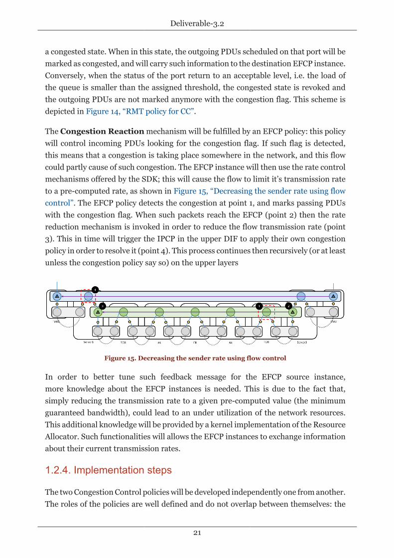
The Congestion Reaction mechanism will be fulfilled by an EFCP policy: this policywill control incoming PDUs looking for the congestion flag. If such flag is detected,this means that a congestion is taking place somewhere in the network, and this flowcould partly cause of such congestion. The EFCP instance will then use the rate controlmechanisms offered by the SDK; this will cause the flow to limit it’s transmission rateto a pre-computed rate, as shown in Figure 15, “Decreasing the sender rate using flowcontrol”. The EFCP policy detects the congestion at point 1, and marks passing PDUswith the congestion flag. When such packets reach the EFCP (point 2) then the ratereduction mechanism is invoked in order to reduce the flow transmission rate (point3). This in time will trigger the IPCP in the upper DIF to apply their own congestionpolicy in order to resolve it (point 4). This process continues then recursively (or at leastunless the congestion policy say so) on the upper layers

Figure 15. Decreasing the sender rate using flow control

In order to better tune such feedback message for the EFCP source instance,more knowledge about the EFCP instances is needed. This is due to the fact that,simply reducing the transmission rate to a given pre-computed value (the minimumguaranteed bandwidth), could lead to an under utilization of the network resources.This additional knowledge will be provided by a kernel implementation of the ResourceAllocator. Such functionalities will allows the EFCP instances to exchange informationabout their current transmission rates.

1.2.4. Implementation steps

The two Congestion Control policies will be developed independently one from another.The roles of the policies are well defined and do not overlap between themselves: the

Deliverable-3.2

22

congestion detection will reside in the RMT and will mark the PDUs using the ExplicitCongestion Notification while the EFCP policy will react to ECN marked packets (whichcan be marked also by other policies, if someone need to develop a different congestionnotification mechanism) and apply a rate control over the flow affected by congestion.

Notice how the RMT policy can be used in all scenarios where it is necessary to react topotential congestion events. Similarly, the EFCP congestion mitigation policy devisedin this section can be used separately from the RMT policy in order to enforce a certaintransmission rate for a flow. The side-effect of this design choice is that the two policiescan be effectively reused by project partners or third parties, maximizing code reuse.

We envision the following roadmap for the implementation phase:

The first step will be to implement the RMT policy which has to detect congestionoccurring in the network. Such policy will organize the queues per port, and willmonitor their states in order to avoid the queue to exceed a threshold (which will bedefined statically or be computed dynamically based on the maximum queue size).Once the threshold for a queue is exceeded, then the port enters in a congested state:traffic outgoing from this port will be marked as congested using the ECN flag inthe PDU’s header. If the queue returns back to acceptable levels (under the definedthreshold) then the port exits from the congested state, and PDUs are no longer markedas congested.

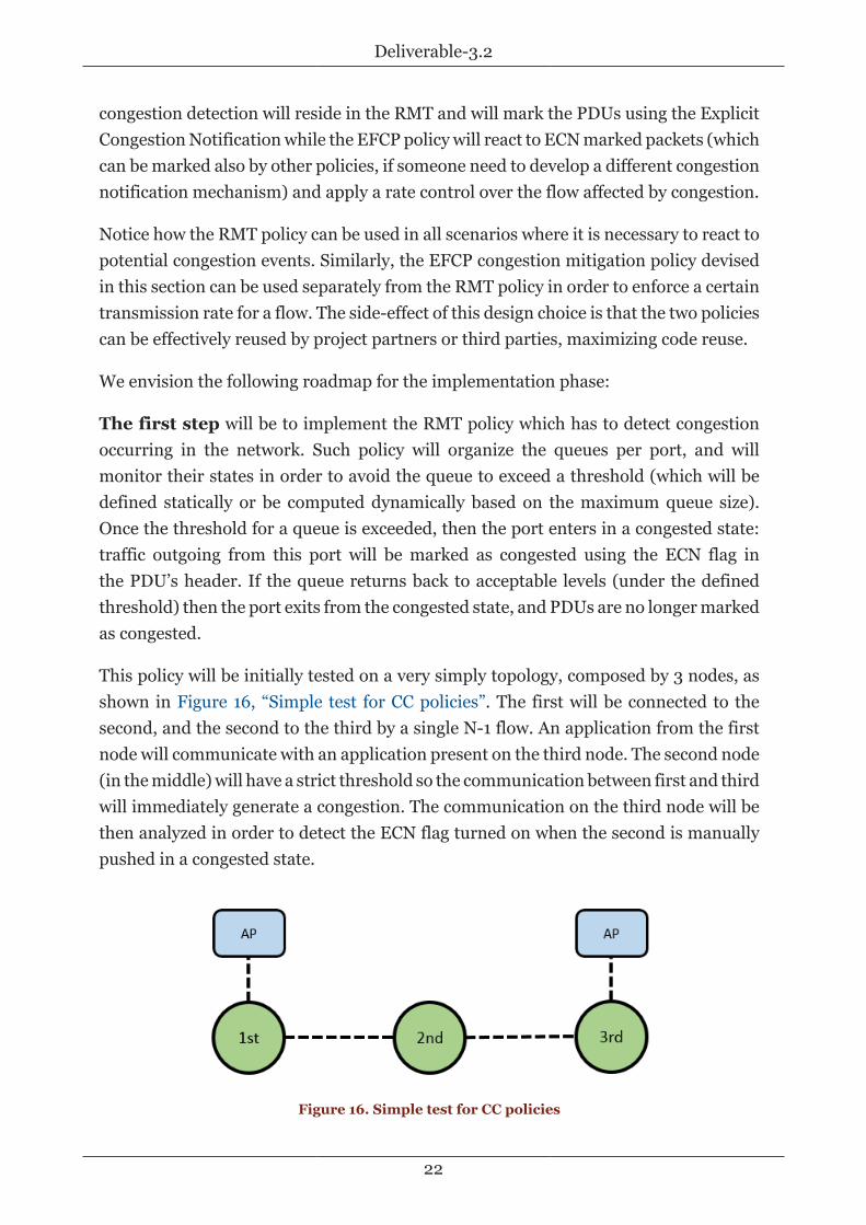
This policy will be initially tested on a very simply topology, composed by 3 nodes, asshown in Figure 16, “Simple test for CC policies”. The first will be connected to thesecond, and the second to the third by a single N-1 flow. An application from the firstnode will communicate with an application present on the third node. The second node(in the middle) will have a strict threshold so the communication between first and thirdwill immediately generate a congestion. The communication on the third node will bethen analyzed in order to detect the ECN flag turned on when the second is manuallypushed in a congested state.

Figure 16. Simple test for CC policies

Deliverable-3.2

23

The second step will be introducing an EFCP policy which reacts to ECN markedincoming PDUs. When a packets with such characteristic is detected, then the EFCPknows there’s a congestion in the network. Such policy will impose a differenttransmission rate to the flow in order to lower the network loads.

This policy will also be initially tested on the same simple topology as seen before.Once the third node receives the ECN-marked PDU then it will use the flow controlmechanism offered by the stack to reduce the flow transmission rate. The first node willbe analyzed in order to detect the rate reduction command and effects.

The last step will take place when a base testing on the policies ensure that theybehave as described by the design requirements. The DC experiment will be swapped-in in the VWall testbed as described in [D61], and the Congestion Control policies willbe assigned at the DC-DIF layer. A series of experiments will be then run on the topof Tenant DIF spawned over DC DIF in order to cause congestion and measure thereaction of the IPCPs in the DIF to it.

Deliverable-3.2

24

2. Resource Allocation

2.1. Traffic differentiation via delay-loss multiplexing policies

This section analyzes two distinct approaches for scheduling and forwarding differenttypes of traffic within a DIF, primarily focusing on the delay and loss requirements ofthe flows, while drafting policies for the relevant RINA components to this task.

2.1.1. Flow cherish and urgency

In scheduling, assigning a higher priority to a flow implies serving its packets beforethan others’, thus keeping its delay lower than that of flows with lower priority. Ina similar way, having a higher threshold on compound queue occupation (numberof packets on all the queues that goes to the same port) ensures, in a congestedenvironment, that a flow will start to have losses due to full buffers later than flows withlower thresholds.

While these priorities and thresholds do not provide a fair distribution of resourcesbetween the distinct flows, they provide an easy and fast way to perform flowdifferentiation given their urgency (requirement of low delay) and cherish (requirementof having low losses). If we consider these two parameters separately and not strictlyrelated as in traditional scheduling approaches (like in Weighted Fair Queuing, WFQ),finer distinction of QoS classes can be achieved. For example, we could effectivelysupport QoS classes desiring low delays but allowing more losses, others targeting lowerlosses but allowing some additional delay, etc. Such a distinction between delay and lossoffers an additional degree of freedom to the scheduling discipline, and thus providingbetter discrimination between different flow requirements in terms of QoS.

Working toward an efficient scheduling discipline to be incorporated in RINA IPCprocesses that effectively accounts for both delay and losses, in this deliverable wefirstly analyze the functionalities that would have to be incorporated to implement theΔQ approach [Davies], as well as the specification of the IPCP policies that would haveto be programmed. As we will highlight, the complete ΔQ approach entails significantcomplexity. Hence, we leave its full implementation for the second iteration of thePRISTINE Project, while in the first one we contemplate simplified Delay/Loss andEnhanced Delay/Loss scheduling schemes. As we show later on by simulation results,such scheduling schemes effectively provide delay and loss differentiation among thesupported QoS classes, and thus will be prototyped as an initial QoS differentiationsolution for RINA DIFs using the PRISTINE SDK. Then, in the second iteration of

Deliverable-3.2

25

the project, these solutions will be subsequently empowered, so as to finally behave asdefined in the complete the ΔQ approach.

2.1.2. The ΔQ approach to QoS

ΔQ is a scheduling model proposed by the company Predictable Network Solutions,based on the idea that a triad of parameters (bandwidth usage, delay and losses)determine the behavior of flows and, by fixing one of these parameters (bandwidthtypically), it is possible to provide efficient treatment and predictable QoS experienceto the others. The ΔQ scheduling module consist in a set of sub-modules (see the Figurebelow for a simplified view):

• Queue Manager: It is the queue management module that manages the usage ofavailable buffers, maintains the distinct queues (using pointers to those buffers) andensures that data on buffers is maintained until sent to all required ports (sendingpackets on multicast only requires one buffer per packet) or dropped.

• Policer/Shaper (P/S): This module has two different functionalities. It ensuresthat flows do not exceed the resource utilization contracted in their servicelevel agreement and also shapes them in order to smooth transient data bursts.Specifically, on the policer side, it controls the maximum bandwidth usage foreach flow and selects the cherish/urgency for each packet, in order to ensure therequirements of the flow. On the shaper side, a small/random delay is addedbetween the packets of a flow in order to smooth burst of data while avoiding thestarvation of low urgency flows.

• Flow Selection: The flow selection module is responsible for forwarding packetsto the distinct P/S depending on their headers. At this point, packets can be dropped(if no valid P/S is found, unknown next hop) or forwarded to one or multiple P/S(depending if they are multicast flows).

• Cherish/Urgency Multiplexer: This module process the packets received fromthe distinct P/S and process them strictly depending on their cherish/urgencyvalues. First, when receiving packets, it decides whether to drop them dependingon the cherish value of the flow and the number of packets waiting to be sent onthat port. Then, when the port is ready to send new data, it selects the next packetto be sent, given the urgency of the supported flows. Since the urgency value canbe degraded for some packets in order to adjust the average delay of the flow, it isimportant to ensure that the order between PDUs of the same flow is maintained.

Deliverable-3.2

26

Figure 17. Simplified view of ΔQ sub-modules.

In more detail, the following features become key to the proper ΔQ operation:

• At the Policer/Shaper (P/S) before the multiplexer:

◦ Flow bandwidth/ratio control. To impose limitations when serving urgentflows in order to avoid starvation of low urgency flows under high congestion.Moreover, bandwidth limitations per QoS are required between domains in orderto avoid that flows originated in one domain saturate the second domain withurgent flows.

◦ Packet spacing. To perform smoothing of data bursts to more constant rates,while adding small variable inter-PDU delays helping to avoid starvation of lowurgency flows/QoS.

◦ Flow degradation. To degrade the QoS class of PDUs belonging toflows consuming more resources than those initially agreed. This measurecomplements the ratio control, degrading the service that PDUs experience whenapproaching the situation that will cause them to be dropped

• At the multiplexer:

◦ Drop PDUs of uncherished flows upon congestion. Depending on the outputport buffer occupation, PDUs of uncherished flows are dropped leaving morespace to PDUs cherished flows. As the buffer occupation increases, the range ofcherished classes with losses also increments, allowing for the most cherishedflows to avoid losses until the very end.

◦ Serve PDUs depending on their urgency. PDUs of more urgent flows are alwaysserved before those with lower urgency value, thus ensuring lower delay onurgent PDUs.

Deliverable-3.2

27

2.1.3. Adaptation of the ΔQ approach to RINA

From the RINA IPCP architecture and operation point of view, the aforementioned ΔQfeatures can be viewed as:

• Limit Flow rate on input port per flow, QoS or Cherish/Urgency class.

• Space PDUs on input ports.

• Degrade flow, QoS or Cherish/Urgency class of PDUs upon resource overuse.

• Cherish/Urgency Multiplexing on output ports.

While ΔQ works "per flow", it leaves the definition of flow quite open (same src/dst +qos, same dst + qos, same dst port + qos, etc.). Given that, while ΔQ perfectly fits aconnection-oriented scenario treating N-level flows individually, we plan to focus ona connectionless approach, where "flows" are defined by a certain IPCP output portand cherish/urgency values (note that multiple QoS Cubes can have the same cherish/urgency values).

ΔQ scheduling will be performed between 3 RMT policies: Scheduling Policy, MaxQPolicy, Q Monitor Policy.

Figure 18. RINA policies related to the ΔQ adaptation

2.1.3.1. Scheduling Policy

This policy is in charge of deciding what Queue must be served next, and is called anytime a PDU is successfully inserted into a queue (not dropped) or the port/RMT core

Deliverable-3.2

28

is ready to process a new PDU and some are waiting in its queues. In ΔQ scheduling inRINA, this policy queries the Monitor policy for the next queue to serve and serves thenext PDU of it. In case of input ports, if the monitor responds to the query of next queueto serve with a NULL Queue pointer, the scheduling policy requests the next servingtime computed for that given port and schedules a new call at that time.

2.1.3.2. Max Q Policy

This policy is responsible for deciding if the last inserted PDU in a queue has to bedropped or not. In ΔQ scheduling in RINA, this policy queries the Monitor policy forPDU dropping probability of that queue, and decides, according to this probability, todrop the PDU randomly.

2.1.3.3. Q Monitor Policy

The Monitor policy of ΔQ is the core of the ΔQ scheduling in RINA. This policy isresponsible for monitoring bursts of bandwidth usage at each input port queue inorder to limit the bandwidth usage of input flows, thus spacing PDUs in this way. Italso monitors output ports, computing how PDUs are sent based on their urgency andarrival time and decides when to degrade the urgency of individual PDUs in the queuesif exceeding the agreed data rate.

The Configuration parameters for this policy are:

• bool LimitIn. If true, enable BW control on input.

• bool space. If true, enable spacing on input.

• bool degradation. If true, enable degradation of urgency on output.

• map<Queue, int >* queueUrgency. Default urgency/priority of an output queue.

• map<Queue, vector< pair< int, double[0..1] > > >* dropOutProb. Probability ofdegrading the urgency in an output queue, given the total number of PDUs waitingto be served in the output port.

If LimitIn is enabled:

• map<Queue*, vector< pair< int, double[0..1] > > > inRates. Rate in which an inputQueue is served, given the number of PDUs waiting to be served at future time.

• map<Queue*, vector< pair< int, double[0..1] > > > dropInProb. Probability ofdropping messages from an input queue, given the number of PDUs waiting to beserved at future time.

Deliverable-3.2

29

If space is enabled:

• map<Queue*, vector< pair< int, pair< double, double > > > > inSpaces. Range ofdelays to space PDUs on an input queue depending on the number of PDUs waitingto be served at future time.

If degradation is enabled:

• map<Queue*, vector< pair< int, double[0..1] > > > outRates. Rate in which anoutput Queue is served, given the number of PDUs waiting to be served at futuretime.

• map<Queue*, vector< pair< int, double[0..1] > > > degOutProb. Probability ofdegrading the urgency in an output queue, given the number of PDUs waiting to beserved at future time.

In the following lines, the targeted functionality (when all procedures are enabled) isbriefly described:

• When a PDU arrives at an input queue: Check the number of PDUs with computedserving time after the current for that queue and get the current rate from inRatesand range of delay from inSpaces. Compute the serving time for the inserted PDUgiven the last computed time and the rate, and the expected serving time given therange of delay and the computed for the last PDU. Also remove all the computedserving times for that queue with already passed.

• When a PDU is dropped from an input queue: Remove the last computed servicetime and expected serving time for that queue.

• When a PDU departs from an input queue: Remove the first computed expectedservice time for that queue.

• When queried for the drop probability of an output queue at input: Check thenumber of PDUs with computed service time after current time for that queue andget the drop probability from dropInProb. Return that probability.

• When queried for the next queue to serve, at input port: Search the queue with thelowest expected service time. If that time is lower or equal than the current time,return it, otherwise return NULL.

• When queried for the next serving time: Search the lowest expected serving timeand return it.

• When a PDU arrives at an output queue: Check the number of PDUs with computedservice time after the current time for that queue and get the probability of

Deliverable-3.2

30

degradation and current rate from degOutProb and outRates. Get the defaulturgency for the queue from queueUrgency, and degrade it (urgency -1) randomly,given the probability of degradation obtained from degOutProb. Put a pointer to thequeue into a priority queue of Queue pointers, with the urgency as priority value.Compute the serving time for the inserted PDU given the last computed time andthe rate.

• When a PDU dropped from an output queue: Remove the last queue pointer insertedfor that queue. Remove the last computed service time for that queue.

• When queried for the drop probability of an output queue at output: Check thenumber of PDUs with computed service time after the current for that queue andget the drop probability from dropOutProb. Return that probability.

• When queried for the next queue to serve, at output port: Extract the first Queuepointer from the priority queue of Queue pointers and return it.

2.1.4. Delay/Loss Scheduling - Cherish/Urgency Multiplexing

As illustrated in the previous section, the complete ΔQ implementation entailssubstantial complexity in the RINA IPCP policies. While the complete ΔQimplementation in RINA is our ultimate goal at the end of the PRISTINE seconditeration, in the first iteration we have implemented and evaluated using the RINAsimulator simpler policies for basic cherish/urgency multiplexing within RINA, whichcan be seen as a first step toward the complete ΔQ implementation goal.

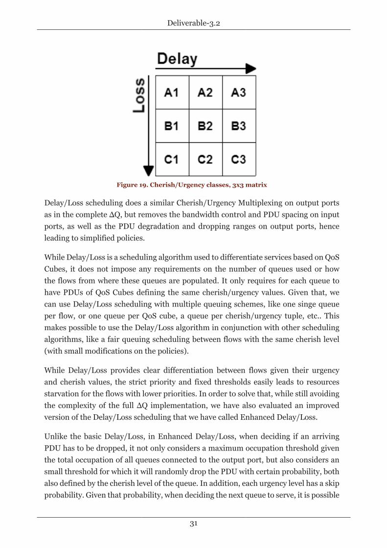
Delay/Loss queuing is a simple scheduling algorithm that mixes priority queuescheduling with distinct thresholds in order to make a strict differentiation of servicesbased on urgency and cherish of flows. In Delay/Loss, cherish/urgency class is assignedto each output queue given the QoS Cube assigned to the PDUs of that queue. For eachcherish/urgency class, the scheduling algorithm can ensure a maximum and averagedelay and losses given a normal usage of the network (at most 100% usage plus bursts,not only urgent/cherished flows, etc.).

Deliverable-3.2

31

Figure 19. Cherish/Urgency classes, 3x3 matrix

Delay/Loss scheduling does a similar Cherish/Urgency Multiplexing on output portsas in the complete ΔQ, but removes the bandwidth control and PDU spacing on inputports, as well as the PDU degradation and dropping ranges on output ports, henceleading to simplified policies.

While Delay/Loss is a scheduling algorithm used to differentiate services based on QoSCubes, it does not impose any requirements on the number of queues used or howthe flows from where these queues are populated. It only requires for each queue tohave PDUs of QoS Cubes defining the same cherish/urgency values. Given that, wecan use Delay/Loss scheduling with multiple queuing schemes, like one singe queueper flow, or one queue per QoS cube, a queue per cherish/urgency tuple, etc.. Thismakes possible to use the Delay/Loss algorithm in conjunction with other schedulingalgorithms, like a fair queuing scheduling between flows with the same cherish level(with small modifications on the policies).

While Delay/Loss provides clear differentiation between flows given their urgencyand cherish values, the strict priority and fixed thresholds easily leads to resourcesstarvation for the flows with lower priorities. In order to solve that, while still avoidingthe complexity of the full ΔQ implementation, we have also evaluated an improvedversion of the Delay/Loss scheduling that we have called Enhanced Delay/Loss.

Unlike the basic Delay/Loss, in Enhanced Delay/Loss, when deciding if an arrivingPDU has to be dropped, it not only considers a maximum occupation threshold giventhe total occupation of all queues connected to the output port, but also considers ansmall threshold for which it will randomly drop the PDU with certain probability, bothalso defined by the cherish level of the queue. In addition, each urgency level has a skipprobability. Given that probability, when deciding the next queue to serve, it is possible

Deliverable-3.2

32

to skip queues with higher urgency, thus giving room to serve PDUs of queues withlower urgency.

2.1.4.1. Draft policies

Delay/Loss scheduling requires the joint collaboration of the 3 RMT policies:Scheduling Policy, MaxQ Policy, Monitor Policy.

Scheduling policy

This policy is in charge of deciding what Queue serve next and is called any time a PDUis inserted into a queue (and not dropped). In Delay/Loss and Enhanced Delay/Lossscheduling in RINA, this policy queries the Monitor policy for the next queue to serveand serves the next PDU waiting there.

Max Q policy

This policy is in charge of deciding if the last inserted PDU in a queue has to bedropped or not. In Delay/Loss and Enhanced Delay/Loss scheduling on RINA, thispolicy queries the Monitor policy for the tuple <occupation, threshold, dropProb,absThreshold> for a given queue, and then it decides if that PDU must be dropped. Thepseudo-code for dropping decision is presented as follows:

if (occupation > absThreshold ) => Drop PDU

else if (occupation > threshold and rand() < dropProb ) => Drop PDU

else => Accept PDU

Monitor policy

The Monitor policy is the core of the Delay/Loss and Enhanced Delay/Loss schedulingin RINA. This policy is responsible for monitoring the usage at each output port and forcomputing how PDUs are sent based on their urgency and arrival time. PRISTINE hasworked in two variants of this policy: delay/loss monitor and enhanced delay/loss monitor. A brief sketch of its functionality is presented as follows:

• When a PDU arrives at an input queue: insert the queue into a queue of Queuepointers.

• When a PDU is dropped from an input queue: remove the last Queue pointer.

• When a PDU departs from an input queue: do nothing.

• When queried for the drop probability of an output queue at an input port: returnthe tuple <queue.length, queue.threshold, 1, queue.threshold>.

Deliverable-3.2

33

• When queried for the next queue to serve at an input port: extract the first Queuepointer from the queue of Queue pointers and return it.

• When a PDU arrives at an output queue: get the urgency for the queue. Put a pointerto the queue into a priority queue of Queue pointers, with the urgency as priorityvalue. Increment the PDU count for that port.

• When a PDU is dropped from an output queue: remove the last queue pointerinserted for that queue. Decrement the PDU count for the port.

• When PDU departs from an output queue: decrement the PDU count for the port.

• When queried for the drop probability of an output queue at output.

◦ With the Delay/Loss scheduling: Check the number of PDUs waiting on the portof the given queue. Get the threshold for that queue. Return the tuple <waitingpdus, threshold, 1, threshold>.

◦ With the Enhanced Delay/Loss scheduling: Check the number of PDUs waitingon the port of the given queue. Get the threshold, drop probability and absolutethreshold for that queue. Return the tuple <waiting pdus, threshold, dropprobability, absolute threshold>.

• When queried for the next queue to serve, at output port.

◦ With the Delay/Loss scheduling: Extract the first Queue pointer from thepriority queue of Queue pointers and return it.

◦ With the Enhanced Delay/Loss scheduling: Search the first urgency with PDUsto serve. Given the probability to skip that urgency, decide to serve it or skipit. If skipped, search for the next urgency with PDUs to serve, and repeat, untilselecting the next urgency to serve. Finally, extract the first Queue pointer fromthe priority queue of Queue pointers with the selected priority and return it.

2.1.5. Simulation results

Some simulations have been obtained using the RINA sim in order to evaluate theperformance of the Delay/Loss and Enhanced Delay/Loss scheduling policies. Theobtained results are presented throughout this section.

2.1.5.1. Delay/Loss vs Best Effort

The first tests that we have conducted are intended to compare the basic Delay/Lossscheduling, with only two levels of cherish and urgency, against a benchmark BestEffort scheduling, with only a single shared queue per output port. For these tests,

Deliverable-3.2

34

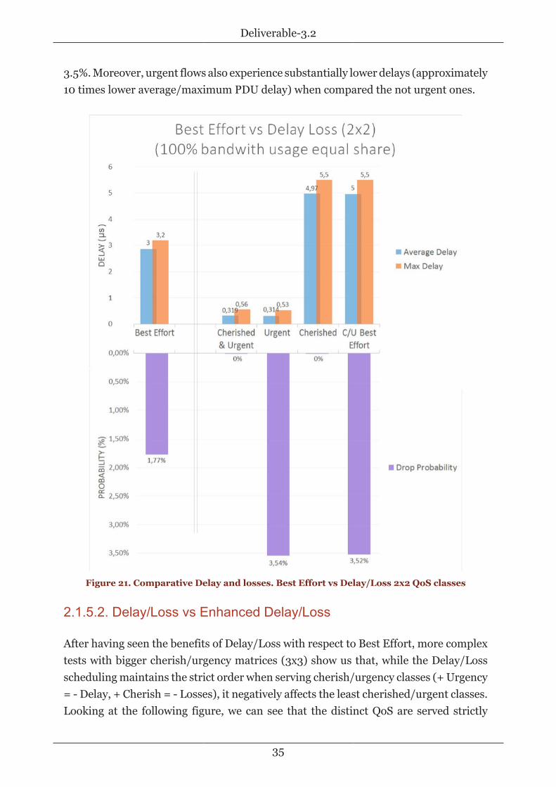
illustrated by the Figure below, our scenario was a simple network with one router,one server and 4 PCs that communicate with the server. In this case, the PCs run 4applications each, each application sending a flow of data consuming nearly 25% ofthe bandwidth from PC to router, each with distinct QoS requirements (Urgent andcherished<A1>, Urgent<B1>, Cherished<A2> and Best Effort<B2>). From router tohost we provision 4 times the bandwidth that we have from the PCs to the router, sothere are 2 bottlenecks in the network (PCs#router and router#server). The generateddata flows are assumed to be bursty, following an ON-OFF traffic profile. ON trafficperiods are composed of 1 to 10 PDUs (uniformly distributed) having each one a size of1024 bits (+/- 400 bits, uniformly distributed) + headers. OFF (i.e., idle) traffic periodsare also assumed to have duration equal to the duration of the complete previous burst.In any case, we would like to mention here that these assumed traffic profiles allow us toperform an initial evaluation of our QoS scheduling proposals. For the final simulationresults, however, we plan to generate more realistic traffic profiles, tightly following thetraffic behaviour of real data applications (HTTP, VoIP, etc.).

Figure 20. Scenario for Delay/Loss 2x2 testing.

The results of the tests are presented in the following figure. While in best effortwe encounter high losses and delay (Round Trip Time, RTT, delays are measured,assuming 0 ms link propagation times, thus only accounting for buffering delays) for allflows, no matter what their QoS requirements are (i.e., no differentiation between themis made), in Delay/Loss we can appreciate that differentiated treatment is provided tothe flows belonging to the different QoS classes, effectively providing their delay andloss demands. As seen, losses are avoided for the cherished flows (PDU loss probability0%), compared to the 1.77% PDU loss probability observed in the best effort scenario.Of course, ensuring such a low PDU loss probability for the cherished flows comes atexpenses of increased losses experienced by the uncherished flows, rising up to around

Deliverable-3.2

35

3.5%. Moreover, urgent flows also experience substantially lower delays (approximately10 times lower average/maximum PDU delay) when compared the not urgent ones.

Figure 21. Comparative Delay and losses. Best Effort vs Delay/Loss 2x2 QoS classes

2.1.5.2. Delay/Loss vs Enhanced Delay/Loss

After having seen the benefits of Delay/Loss with respect to Best Effort, more complextests with bigger cherish/urgency matrices (3x3) show us that, while the Delay/Lossscheduling maintains the strict order when serving cherish/urgency classes (+ Urgency= - Delay, + Cherish = - Losses), it negatively affects the least cherished/urgent classes.Looking at the following figure, we can see that the distinct QoS are served strictly

Deliverable-3.2

36

following their requirements (Cherish (A) has less losses than Low Cherished traffic(B) and that less than Uncherished ©, and Urgent (1) has less delay than Low Urgency(2) and that less than Not Urgent (3)), there is really no feasible way of adjust howthe distinct QoS are served, ending with really similar delays / losses in all the classesexcept in the Non Urgent / Uncherished ones.

Figure 22. Comparative Delay and losses. Delay/Loss 3x3 QoS classes

These large differences between QoS cubes using the Delay/Loss scheduling were themotivation behind the proposal of the Enhanced Delay/Loss one. To highlight thebenefits of the latter, we compare their behavior in a similar scenario as before. Inthis case, our scenario was built using 2 PCs interconnected, each with 45 pairs ofapplications communicating between them. Among these 45 pairs of applications, 9groups of 5 applications were assumed, each group of applications requesting flows of acertain QoS class (from the 9 available in the 3x3 QoS class matrix). In order to simulatea realistic scenario, bandwidth usage between the distinct QoS was divided in a waythat ~5% of the traffic was urgent, ~40% had low urgency and the remaining ~55% wasnon-urgent.

We have tested the same scenario with Enhanced Delay/Loss. In this case, giventhe extra possibilities of Enhanced Delay/Loss, we configured it with the idea of, interms of urgency, provide to urgent classes the same minimum delay as before, butdistribute the delay between less urgent flows in a fairest way. The same was done forthe experienced PDU losses, remaining the highest cherished QoS cubes without losseswhenever possible, and then distribute them fairly between the least cherished QoS.The next figure show the results obtained for the Enhanced Delay/Loss scheduling. In

Deliverable-3.2

37

the plotted bar graphs, we can see that, in addition to maintain the strict distinctionbetween how the QoS are served depending of their cherish/urgency values, the resultsobtained show a scenario where the distinct QoS becomes clearly distinguished, but thedifferences between Uncherished / Non urgent and the rest of classes are not so abrupt.

Figure 23. Comparative Delay and losses. Enhanced Delay/Loss 3x3 QoS classes

Figure 24. Configuration example for RINA sim. Left: ini file for Delay/Loss and Enhanced Delay/Loss. Right: xml for Enhanced Delay/Loss

2.1.6. Next Steps

Delay/Loss policies have shown good results in controlled environments like the onessimulated with RINA sim. Thus, our next step will be to prototype them using thePRISTINE RINA SDK. In addition, we are going to continue the work with the morecomplex scheduling that ΔQ. For that, we are going to do the full implementation in theRINA sim in order to finish adjusting the distinct policies and test its behavior. At theend, we expect to implement a complete and configurable set of ΔQ scheduling policieswithin the RINA SDK.

Deliverable-3.2

38

2.2. QoS-aware Multipath Routing

2.2.1. Multipath Routing Overview

Multipath routing refers to routing strategies in which traffic is delivered throughmultiple paths. Sender or intermediate nodes have several next-hops for a givendestination and must choose the next-hop for a given packet. Multipath routing isused for performance and traffic engineering purposes such as load balancing orcongestion avoidance among others. In the following we outline common multipathrouting strategies.

2.2.1.1. Equal Cost Multi-Path (ECMP)

Equal-cost multi-path routing (ECMP) is a routing strategy that distributes trafficamong equal-cost routes to the same destination, typically using Round Robin orrandom approaches. ECMP is a per-hop decision that is limited to a single router. It isused for load balancing, also offering increases in bandwidth.

ECMP presents the drawback of variable latency among the paths causing packetsto arrive out of order, increasing delivery latency and buffering requirements. Thisproblem arises when packets in the flow are split among multiple paths. Therefore, toavoid this situation the natural solution is to deliver packets belonging to the same flowthrough the same path. [RFC2991] describes some solutions for a router to select thesame path (next-hop) per flow, namely: Modulo-N Hash, Hash-Threshold and HighestRandom Weight. These solutions rely on some form of hash function.

ECMP always split traffic evenly among the available paths, which is not the optimalsolution for variable and non-balanced scenarios. Weighted ECMP aims to address thisproblem.

2.2.1.2. Weighted ECMP

Weighted ECMP is a form of ECMP which distributes traffic among paths based on a setof pre-determined ratios. Heuristics are used to find optimal traffic distribution (linkweights) based on source routing approaches (explained below).

However, [Chiesa] demonstrates that optimizing link weight configuration or evenachieving a good approximation to the optimum is an infeasible task, which is a hugedrawback for weighted ECMP.

Deliverable-3.2

39

2.2.1.3. Source routing

Source routing is a routing strategy by which the sender partially or completely specifiespackets’ route.

In strict source routing, the sender specifies the exact route the packet must take, butthis is never used in practice. Loose Source Record Route (LSRR) is more commonlyused, in which the sender gives one or more hops that the packet must go through.

Source routing allows a network manager to perform the routing functionality anddecide the routes the traffic traverses. Also, alternate links can be used upon changingconditions, for example to avoid congested links.

2.2.1.4. Policy-based routing

Policy-based routing (PBR) is a routing strategy that makes routing decisions based onpre-defined policies. This allows forwarding packets based on varied criteria such as thesource address instead of the destination address, the size of the packet, the protocolof the payload, or other information available in a packet header or payload.

2.2.1.5. Dynamic Adaptive Routing

Adaptive routing is a common characteristic of routing protocols such as RIP or OSPF,which refers to the ability to alter the path that the route takes through the system inresponse to a change in conditions. For example, if a certain node crashes, anotherfeasible path (if any) is discovered and chosen by the protocol to reach the affecteddestinations. The opposite of adaptive routing is static routing, in which the paths arefixed and failures in them leads to connection breaks.

Dynamic Adaptive Routing aims to react upon dynamic conditions such as linkcongestion level, i.e. choosing the best paths based on dynamic conditions that damageQoS. This kind of multipath routing is so far not well studied, being only addressedin highly variable networks such as sensor networks or heterogeneous networks(HETNETs). Besides, its implementation poses many challenges mainly due to thedifficulty of cross-layer optimization between the transport and network layer.

2.2.2. QoS-aware multipath routing

A general drawback presented by the existing multipath solutions is that applicationrequirements are not considered. This leads to non-optimal multipath solutions sincesome applications are delay-, jitter- and loss-sensitive, and therefore not suitable for

Deliverable-3.2

40

multipath approaches, while others are not sensible to these parameters and maybenefit greatly of the extra bandwidth achieved by using multiple available paths.

As an example, video conference applications are very sensible to delay and jitter,and therefore require a single path approach to avoid packet reordering and bufferingdelays. In contrast, file transfer applications just need bandwidth to deliver the contentas fast as possible, and do not care about delay and jitter.

Therefore, considering the application QoS requirements when taking the decision ofwhether to do multipath or not, or deciding how many paths to split the traffic among,can lead to consistent benefits in terms of performance and quality perceived by theend-user.

2.2.2.1. Multipath level

The next figure outlines a tentative arrangement of different application typesaccording to their “optimal” multipath level, i.e. the number of available paths theyshould use to deliver optimal performance. This is just an exercise to show theimportance of the application requirements in multipath routing and the figure doesnot show experimental results of any kind.

Figure 25. Multipath level

For delay- and jitter-sensitive applications such as video conference and audio calls,the most appropriate approach might be to use a single path. However, in casethe delay variance and re-ordering delay overhead keep under the delayQoS requirements, multiple paths can be also used without affecting therequired performance.

Deliverable-3.2

41

Bandwidth-demanding applications such as buffered multimedia or video streamingmay benefit of the bandwidth obtained by means of multiple paths, but always keepingan eye on the multipath drawbacks on QoS parameters such as delay, jitter and packetlosses, which may require the utilization of less (or even a single) paths. Web trafficcan benefit largely from multipath, since web browsers gather the different web objectsusing separate connections and multiple paths can be leveraged. Some web contentmay require high bandwidth, however the bandwidth requirements are not that highas for multimedia applications and the maximum multipath level can be maintainedbelow theirs. Finally, bandwidth demanding applications which have not delay, jitter orpacket loss requirements may benefit greatly from a high multipath level. For examplefile transfer applications. They may use the maximum bandwidth provided by thedifferent available paths to transmit the content as fast as possible. However, in somecases using all the available paths may have additional drawbacks. Especially when thenumber of available paths is very high, and the forwarding through all of them shallbe avoided.

2.2.2.2. When to do multipath?

Current multipath routing solutions are applied in a pre-defined way. Network nodesalready have a pre-defined multipath level to follow, and the question of whether toperform multipath or not is never asked nor answered. For example, network nodesmay have an ECMP routing strategy installed, and they will always spread traffic amongpaths.

Weighted ECMP allows some degree of configuration by means of dynamically varyingthe link weights, but this is more oriented to dynamic load balancing rather than takinga true decision on whether to perform multipath or not. A true dynamic weighted ECMPcan serve as the basis to achieve dynamic configurations of different multipath levels.For example, a link weight of zero may indicate that traffic is not to be forwardedthrough it, and in case this link is allowed for multipath, its weight can be changed.However, this approach also carries the drawback of not considering the kind of trafficthat is being forwarded, since the link weights apply for all the traffic that reaches andleaves a certain node.

Therefore, to take dynamic decisions on whether to perform multipath and whatmultipath level applies, the consideration of the application and differentiation oftraffic type is mandatory. In the following we elaborate how such an approach can beimplemented using RINA.

Deliverable-3.2

42

2.2.2.3. Multipath level

We can define multipath level as a measure that determines the type of multipathrouting strategies associated with the forwarding of a certain traffic type throughdifferent possible paths, which allows taking the decision on what next hop to choosefor each packet.

This measure can be unidimensional or multidimensional depending on the degree ofinformation that it conveys to the policies that take multipath routing decisions. Forexample, a unidimensional measure from 0 to 1 may indicate the desired multipathlevel from a single path (0) to all possible paths (1), or something in between. Anotherpossibility is to use a bi-dimensional measure indicating the previous metric togetherwith the typical deviation of the traffic load to be forwarded through different paths, sothat the major traffic load is concentrated in a reduced number of paths.

Other aspect that may be considered for the multipath level is whether multipath isperformed as long as multiple paths are available, or if multipath takes place uponcertain conditions (e.g. congestion, as MPTCP).

In summary, for specifying the multipath level we can use any multi-dimensionalmeasure that we need to convey the needed information to the routing policies, as longas those policies understand the information that this measure includes.

2.2.2.4. Multipath-based Resource Allocation

Apart from the multipath level, resource allocation is a key aspect for the routingdecisions. In fact, multipath routing can be understood as a way of resource allocation,since routing traffic through a certain path means to utilize or allocate that networkresources for the routed traffic.

The driving paradigm of resource allocation is to optimally utilize the resourcesavailable to it (maintaining the appropriate safety levels), while responding to requestsfor service and satisfying those that it can while still staying within its policy bounds.What resources to allocate to what entity is a matter of the resource allocation approach.QoS-aware multipath routing in this case can be seen as a way of providing furtherinformation to the resource allocation mechanisms to share the available networkresources more efficiently. I.e. the resource allocation mechanisms will know whento dedicate resources of the same link to single path oriented traffic and when toshare link capacity among multi-path oriented traffic. Therefore, the result of theseresource allocation mechanisms is to influence the forwarding decision, which leads toa multipath-based resource allocation approach.

Deliverable-3.2

43

2.2.3. Multipath levels in RINA

In RINA, when a flow request is issued, the QoS requirements are passed to the DIFas part of the flow allocation requests. The QoS requirements are then compared withthe QoS cubes provided by the DIF (each QoS cube can be thought of a set of policiesthat guarantee a specific level of service), and, in case the request can be honored by theDIF, the most appropriate QoS cube is selected. Then, the different policies forward thetraffic to comply with those QoS specifications. Therefore, when an application requestsa flow allocation, its requirements are indicated by means of the QoS parameters. Inorder to determine the multipath level associated with that application, the multipathlevel is derived from the QoS parameters indicated by the application.

Individual applications cannot request what is the multipath level they want for theirflow for two reasons. Applications care about the outcomes of the service the DIFprovides, not about how the service is implemented: if the flow is transported overa single or multiple paths over the DIF is a detail of the service implementation;as long as the DIF guarantees the flow characteristics requested by the application,the application does not care. In other words, the application tells the DIF whatoutcomes it wants, not how to achieve them. The second reason is that the DIFis a black box; the application has no visibility inside, and therefore cannot know thepaths the DIF can use.

2.2.3.1. Derivation of the multipath level from the QoS requirements

The multipath level associated with a certain flow can be derived by means of the QoSrequirements associated to the flow (e.g. jitter, delay, bandwidth, etc.). In fact, this mayimply not considering any multipath level at all, since the multipath decision policiescan take directly the needed QoS parameters to take the decision. We use the multipathlevel concept here for the sake of clarity.

QoS parameters [D22] that can be considered to determine the multipath level are:

• Average bandwidth: Unsigned Integer - measured at the application in bits/sec

• Average SDU bandwidth: Unsigned Integer - measured in SDUs/sec

• Peak bandwidth-duration: Unsigned Integer - measured in bits/sec

• Peak SDU bandwidth-duration: Unsigned Integer - measured in SDUs/sec

Higher bandwidth requirements demand the utilization of additional paths to fulfill therequirements.

Deliverable-3.2

44

• Burst period: Unsigned Integer - measured in seconds

• Burst duration: Unsigned Integer - measured in fraction of Burst Period

Bursts may demand the utilization of single paths. So burst periods and durations mustbe considered to allocate those bursts accordingly among the different possible paths.

• MaxDelay: Unsigned Integer - in secs

The delay may constrain the multipath decision, as the delay varies among paths. Underdelay constraints, some paths might be out of the scope, and therefore the multipathlevel reduced.

• Jitter: Unsigned Integer - in secs

Tight jitter constraints demand low multipath level (including single path). In case ofloose jitter constraints, additional paths may be used freely.

2.2.4. QoS-Aware Multipath Routing for RINA

This section describes how the presented QoS-aware multipath routing and dynamicadaptive routing concepts can be implemented in RINA, studying what RINAcomponents and policies are involved in the multipath routing approach.

The main requirement for forwarding is to take fast decisions (since it is a functionperformed for each PDU). Thus the amount of required computation to forwarda packet should be small. For example, when following a round-robin approach,the computation might consist of incrementing a next-hop index, keeping the delayoverhead at a minimum. This involves low computing overhead, i.e. the amount ofcomputing involved in the forwarding strategy shall be small. The computation ofpaths, next hop to use, etc. shall be carried out fast and in a non-redundant manner. Tothat end, pre-computed data will be stored to be accessed by routing algorithms, thusachieving both optimal routing and fast decisions.

Figure 26, “Multipath routing design” illustrates, from a high-level point of view, thescope of the multipath approach within the involved RINA components, namely theRelaying and Multiplexing Task (RMT), Resource Allocator (RA) and Routing.

Deliverable-3.2

45

Figure 26. Multipath routing design

2.2.4.1. Routing

Routing exchanges connectivity and other state information with other IPC processesof the DIF and holds the routing table generation algorithms. Routing performs theanalysis of the information maintained by the RIB to provide connectivity input for thecreation of the forwarding table. Routing executes when it is needed (periodically, basedon routing updates from neighbors, etc). It computes routes to next hop addresses andprovides this information to the Resource Allocator.

Multipath routing policy

Since routing is computationally expensive, generally is not worth it to executerouting algorithms to take forwarding decisions on a PDU-basis. Instead,routing algorithms are executed with more time granularity, being the results stored inthe PDU forwarding table to be consulted in a fast manner to reduce the forwardingdecision time.

In multipath routing, the output of the Routing component must comprise thedifferent next hop addresses of the existing available paths to reach a certaindestination, including figures of merit associated with each next hop to be usedin the PDU forwarding decision process. Always having in mind that this decisionshould be as fast as possible, the resource allocator must provide the necessary pre-computed information to optimize the forwarding decision time. This is a matterof synchronization between Routing and the PDU forwarding policy to reach the

Deliverable-3.2

46

optimization goal in a coordinated way. For example, Routing may provide informationabout the optimality of each next hop, which can be used in the decision process.

2.2.4.2. Resource Allocator

The Resource Allocator takes the output provided by the Routing component andprovides information to the PDU Forwarding function (for example PDU Forwardingtable entries if this function is table-based). The RA can be distributed, collaboratingwith other RAs in members of the DIF (autonomic approach). The RA can also collectand communicate information to the DIF Management System (traditional approach).The traditional approach is suitable when resources in the members of the DIF aretightly constrained, while the autonomic approach is more suitable when fast reactiontimes are required. In practice, the norm will be somewhere in between.

There are basically three sets of information available to the RA to make its decisions:

• The characteristics of the flows requested by the applications using the DIF via"allocate flow requests".

• The properties of the N-1 flows the DIF is relaying on.

• Information from other members of the DIF on what they are observing (this lattercategory could be restricted to just nearest neighbors or some other subset - all twoor three hop neighbors - or the all members of the DIF). This is carried out by meansof RA-RA communications.

Generally speaking, the RA accounts for the adaptiveness of the multipath routingstrategy, i.e. the dynamic modification of the forwarding table based on changingconditions. This is done by means of the dynamic update of the PDU forwarding table.

PDU forwarding table generator policy

The PDU forwarding table generator policy generates and updates the PDU forwardingtable of the RMT. It takes as input information provided by the ResourceAllocator, which includes aspects related to resource allocation policies.These resource allocation aspects are within the RA’s scope, and may be determined bymeans of RA-RA communications.

2.2.4.3. Relaying and Multiplexing Task

The primary job of the RMT in its multiplexing role is to pass PDUs from DTP instancesto the appropriate (N-1)-ports. PDUs are usually forwarded based on its destinationaddress, and QoS-cube-id fields.

Deliverable-3.2

47

The key component of the RMT for multipath routing is the PDU forwarding policy.

PDU forwarding policy and PDU forwarding table

This policy is invoked per PDU in order to obtain the N-1 port(s) through which thePDU has to be forwarded. It takes forwarding decisions on a PDU-by-PDU basis, sothe delay overhead posed by its execution is a key requirement for a proper forwardingoperation.

The PDU forwarding policy consults the PDU forwarding table, which stores the pre-computed forwarding information. In this way fast forwarding decisions are assuredwithout involving additional computing cost. However, the forwarding policy mayuse additional dynamic information (e.g., queue residency times for the different(N-1) ports) along with the pre-computed forwarding table. Besides, the policy mightmake decisions in some other way than simply blindly using the pre-computed data(e.g., apportioning the traffic to different next-hops using a randomizing selectionalgorithm), but always complying with the tight time requirements.

In the simplest case, the PDU forwarding policy only needs to be passed the addressand QoS cube from the PDU to make its forwarding decisions. However, in a multipathscenario the PDU forwarding policy must make the decision on what available pathuse to forward the traffic. In this case, other information in the EFCP PCI like CEP-idsmight be useful to reduce the incidence of getting PDUs out-of-order at the destination.

2.2.5. A QoS-aware multipath solution for RINA focused onDatacenter Networking

In this section we describe the QoS-aware multipath routing policies for the DatNet usecase. We first start by presenting the DIF structure, and then we proceed to specify thepolicies that apply for the following incremental routing strategies:

• Simple link-state routing, applying Dijkstra’s algorithm to compute the shortestpath.

• Multipath link-state routing, computing a set of different shortest paths and load-balancing the traffic among them.

• QoS-aware multipath link-state routing, enhancing the approach of the previouspoint by considering an intelligent QoS-aware multipath strategy to split the trafficamong all the possible paths optimizing resource allocation while improving thenetwork efficiency.

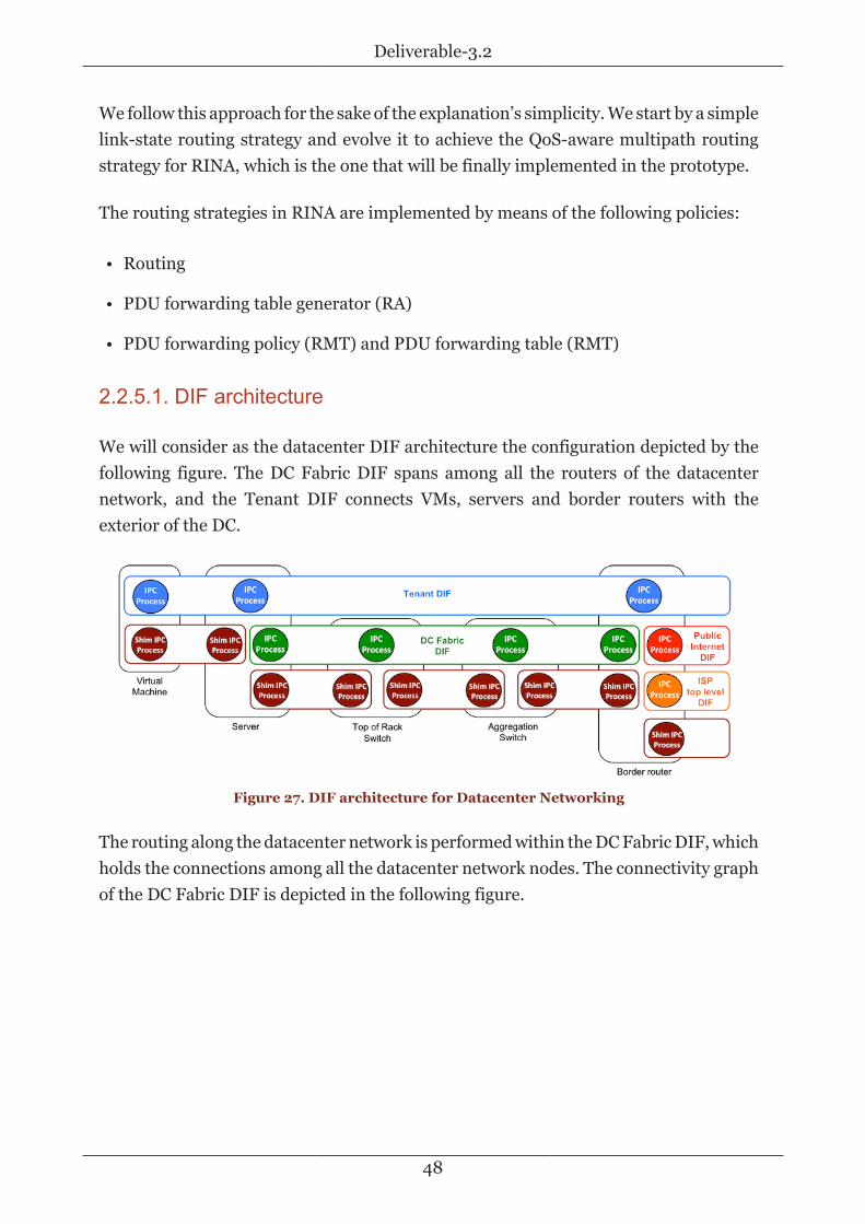
Deliverable-3.2

48

We follow this approach for the sake of the explanation’s simplicity. We start by a simplelink-state routing strategy and evolve it to achieve the QoS-aware multipath routingstrategy for RINA, which is the one that will be finally implemented in the prototype.

The routing strategies in RINA are implemented by means of the following policies:

• Routing

• PDU forwarding table generator (RA)

• PDU forwarding policy (RMT) and PDU forwarding table (RMT)

2.2.5.1. DIF architecture

We will consider as the datacenter DIF architecture the configuration depicted by thefollowing figure. The DC Fabric DIF spans among all the routers of the datacenternetwork, and the Tenant DIF connects VMs, servers and border routers with theexterior of the DC.

Figure 27. DIF architecture for Datacenter Networking

The routing along the datacenter network is performed within the DC Fabric DIF, whichholds the connections among all the datacenter network nodes. The connectivity graphof the DC Fabric DIF is depicted in the following figure.

Deliverable-3.2

49

Figure 28. Connectivity graph of the DC Fabric DIF (S=Server,T=Top of Rack Switch, A=Aggregation Switch, B=Border Router)

2.2.5.2. Simple link-state routing

To start defining the policy design for the QoS-aware multipath routing strategy, let’sfirst start by analyzing a non-multipath strategy such as a simple link-state routingstrategy, which is based on the following process:

1. Each network node determines what other nodes it is connected to and throughwhat ports. It does this using a "reachability protocol" which runs periodically andindependently with each of its neighbors.

2. Each node periodically (and in case of connectivity changes) creates a "link-stateadvertisement" message containing:

• The node which is sending the message.

• The nodes to which the sender is directly connected.

• A sequence number, which is increased every time the source node sends a newlink-state advertisement.

3. The message is flooded throughout the entire network. Each node then storesthe message with the more recent sequence number, so the last link-stateadvertisement quickly gets stored in every node in the network.

4. Each node calculates the network graph iterating over the set of link-stateadvertisements from each node of the network. For a link to be considered ascorrectly reported the two ends must have sent the corresponding link-stateadvertisement. To that end, each node holds two data structures:

• A "network tree" containing the self node as root and the other nodes as branchesand leaves following the "shortest-path" route from the node. The routing tableis formed with the output port that identifies the branch that contains thedestination node.

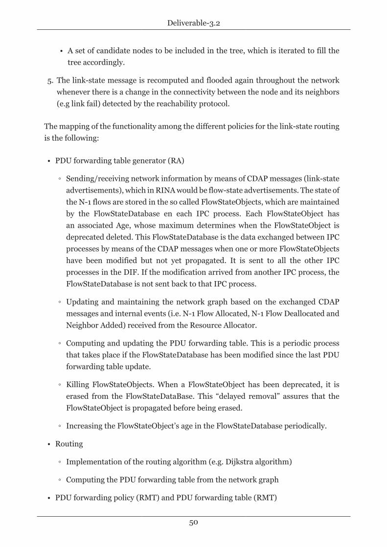
Deliverable-3.2

50

• A set of candidate nodes to be included in the tree, which is iterated to fill thetree accordingly.

5. The link-state message is recomputed and flooded again throughout the networkwhenever there is a change in the connectivity between the node and its neighbors(e.g link fail) detected by the reachability protocol.

The mapping of the functionality among the different policies for the link-state routingis the following:

• PDU forwarding table generator (RA)

◦ Sending/receiving network information by means of CDAP messages (link-stateadvertisements), which in RINA would be flow-state advertisements. The state ofthe N-1 flows are stored in the so called FlowStateObjects, which are maintainedby the FlowStateDatabase en each IPC process. Each FlowStateObject hasan associated Age, whose maximum determines when the FlowStateObject isdeprecated deleted. This FlowStateDatabase is the data exchanged between IPCprocesses by means of the CDAP messages when one or more FlowStateObjectshave been modified but not yet propagated. It is sent to all the other IPCprocesses in the DIF. If the modification arrived from another IPC process, theFlowStateDatabase is not sent back to that IPC process.

◦ Updating and maintaining the network graph based on the exchanged CDAPmessages and internal events (i.e. N-1 Flow Allocated, N-1 Flow Deallocated andNeighbor Added) received from the Resource Allocator.

◦ Computing and updating the PDU forwarding table. This is a periodic processthat takes place if the FlowStateDatabase has been modified since the last PDUforwarding table update.

◦ Killing FlowStateObjects. When a FlowStateObject has been deprecated, it iserased from the FlowStateDataBase. This “delayed removal” assures that theFlowStateObject is propagated before being erased.

◦ Increasing the FlowStateObject’s age in the FlowStateDatabase periodically.

• Routing

◦ Implementation of the routing algorithm (e.g. Dijkstra algorithm)

◦ Computing the PDU forwarding table from the network graph

• PDU forwarding policy (RMT) and PDU forwarding table (RMT)

Deliverable-3.2

51

◦ Forwarding decisions on a PDU basis from the data stored in the PDU forwardingtable, which in this case is a simple table containing mappings of <destination,QoS-id> tuples to outgoing ports.

2.2.5.3. Simple Multipath link-state routing

The next incremental step is to study a multipath strategy derived from the above link-state strategy. A simple case to consider is a multipath strategy which load-balancestraffic among a set of pre-computed shortest paths. The load-balancing functionality,which is within the scope of the PDU forwarding policy, can be defined as a policy,leaving the door open for the implementation of different forwarding strategies amongthe set of shortest paths. In case the traffic is evenly distributed among them, it willbe similar to the Equal Cost Multipath (ECMP) solution typically used in datacenternetworks. However, different policies can be implemented in the PDU forwardingpolicy to spread the traffic among the paths with different distributions.

In our case, for the sake of simplicity, and focusing the feasibility of the multipathstrategies in RINA, we will focus on a ECMP-like case. That is, distributing the trafficevenly among the set of shortest paths. ECMP does so distributing the TCP connections.In this case, this simple multipath routing solution for RINA will distribute PDUsbelonging to different EFCP connections through the multiple N-1 flows.

In this case, the changes of the functionality of the different policies with respect to theprevious case is the following:

• PDU forwarding table generator (RA)

◦ idem.

• Routing

◦ In this case, it is needed a routing algorithm that retrieves the set of shortestpaths. The most direct approach is to consider a "shortest path tree" computedusing the Dijkstra algorithm over the network graph.

◦ As for the computing of the PDU forwarding table from the network graph adifferent approach is needed, since in this case not only a single path is returned,but the set of all the shortest paths.

• PDU forwarding policy (RMT) and PDU forwarding table (RMT)

◦ In this case, the PDU forwarding policy distributes the traffic evenly amongthe different paths. Therefore, the PDU forwarding policy must implement the

Deliverable-3.2

52

necessary mechanisms for that purpose, retrieving the available ports from thePDU forwarding table and distributing the PDUs among them (e.g. in a Round-Robin fashion for the ECMP case).

◦ In this case the PDU forwarding table needs to account for the extra informationneeded to perform multipath. To that end multiple entries for the same<destination, qos-id> pairs will account for the different possible next hops.

2.2.5.4. QoS-aware multipath link-state routing

The previous studied routing strategies (simple link-state and simple multipath link-state) only consider the link state (up or down) and a cost metric (number of hops)to determine the shortest paths and to form the DPU forwarding table accordingly.Here we propose a QoS-aware multipath routing solution that considers also the QoSrequirements of the flows to take the forwarding decisions, i.e., the QoS requirementsof the N flows are considered to forward the traffic through the N-1 flows.

Two different possibilities are considered depending on whether dynamic real-timelink-state (or flow-state) information is available (e.g. link utilization/congestion level,etc.).

Static QoS-aware multipath routing

In the static QoS-aware multipath case, no dynamic link-state information is used andthe only information available per-link is:

• Whether the link is up or down

• Associated cost metric

• Link bandwidth

In this case, the only information to make "QoS-aware forwarding decisions" is toconsider the known QoS requirements of the N-flows to generate the PDU forwardingtable. As a first approach, we will consider the QoS requirements on delay and jitter,and the average bandwidth of the flow as input to the routing algorithm.

Many possibilities are present with regards the routing algorithms in this case. There isa wide range of possibilities when splitting traffic among different paths considering thetraffic characteristics. As a first step for static QoS-aware multipath routing algorithms,we propose a sort of "QoS-driven load-balancing algorithm", in which the flows arespread among the different shortest paths aiming at two objectives:

Deliverable-3.2

53

1. Not overloading the paths. That is, if we have a set of flows with high averagebandwidth and low average bandwidth, the goal is to avoid sending over the samepaths the bigger flows, therefore combining over the same paths big and small flowsso that the paths do not get congested. In the same way, if no feasible way do existto spread the flows among paths so that none of them gets congested, the goal is tominimize the caused overload, constraining it to the minimum number of paths.

2. Sending the data belonging to the same flow over the same path. Thus avoidingreordering delays caused by multipath.

Note that the approach proposed here should not be the optimal one, since otheralgorithms may (and most likely do) have better performance. However, we leave thisaspect for the second part of the project, and for this deliverable we focus on therealization of a feasible static QoS-aware multipath algorithm.

In this case, the changes of the functionality of the different policies with respect to theprevious case is the following:

• PDU forwarding table generator (RA)

◦ Idem.

• Routing

◦ Idem as in the simple multipath case.

• PDU forwarding policy (RMT) and PDU forwarding table (RMT)

◦ In this case, the PDU forwarding policy distributes the traffic among the differentpaths according to the flows' QoS requirements. To that end, the PDU forwardingpolicy in each IPC process must store a record of the following:

▪ Connection to what the PDUs that have reached the IPCP belong to. Thisis identified by the connection endpoints ids (cep-src-id, cep-dest-id) andthe qos-id. This is done to forward the PDUs belonging to the same flowsthrough the same port. Each time an unidentified PDU arrives, the connectionidentifiers are stored and a port is chosen for that PDU. For the next PDUsbelonging to the same connection, they are forwarded through the sameport. A time span is associated with each of the connections, and updatedperiodically. When no PDUs of a certain connection have been forwarded overa certain time span, the connection register is deleted.

▪ Average bandwidth allocated to each port. Each time a port is chosen toforward a PDU, the PDU forwarding policy stores the accumulated averagebandwidth of the connections allocated to that port.

Deliverable-3.2

54

◦ The QoS-aware multipath algorithm implemented by the PDU forwardingfunction consists on the following main steps:

i. When a PDU of a new connection arrives at the IPC process, the PDUforwarding policy checks the set of paths that lead to the destination andretrieves the set of ports that can be used to forward the PDU.

ii. The port with less average bandwidth allocated is chosen, the connectionidentifiers are stored, and the average bandwidth allocated for that port isincremented.

iii.For the next PDUs of that connection, the PDU forwarding policy checksthat it has the connection identifiers already stored, and forwards the PDUsthrough the already allocated port.

iv. When a connection reaches the maximum time without PDUs beingforwarded through that IPC process, the connection identifiers are deletedand the bandwidth allocated to the corresponding port is reduced.

◦ The PDU forwarding table does not change with respect the previous simplemultipath case.

Dynamic QoS-aware multipath routing

In the dynamic QoS-aware multipath case, dynamic link-state information is availablein addition to the previous static per-link information. In this case the availableinformation per link is:

• Whether the link is up or down

• Associated cost metric

• Link bandwidth

• Dynamic monitored information

◦ Instant traffic load/link utilization (where "instant" refers to the last monitoredvalue)

◦ Traffic statistics collected at network level.

In this case, apart from considering the QoS requirements of the N-flows, the dynamicmonitored information can be also used to generate the PDU forwarding table.

Many possibilities are also present in this case with regards the routing algorithms. Thepreviously proposed "QoS-driven load-balancing algorithm" for the static QoS-awaremultipath routing case, can be extended to consider the traffic stats per link and spread

Deliverable-3.2

55

the flows among the different shortest paths aiming at the same two objectives of theabove point:

1. Not overloading the paths. Apart from combining over the same paths big and smallflows, the Dynamic QoS-aware multipath routing approach aims to consider thecongested links to avoid forwarding traffic through them, choosing alternative (andless congested) paths when this situation occurs.

2. Sending the data belonging to the same flow over the same path. Thus avoidingreordering delays caused by multipath.

In this case, the changes of the functionality of the different policies with respect to theprevious case is the following:

• PDU forwarding table generator (RA)

◦ The Resource Allocator, by means of the PDU forwarding table generator mayuse traffic statistics and generate the PDU forwarding table accordingly. Forexample, if a highly congested link is detected, the PDU forwarding tableentries forwarding traffic through that link may be deleted, thus eliminating thepossibility of routing traffic through it. This decisions are to be made on a coarsetime granularity, i.e., when a link is congested for large periods of time.

• Routing

◦ Idem as in the static QoS-aware multipath case.

• PDU forwarding policy (RMT) and PDU forwarding table (RMT)

◦ As in the static case, the PDU forwarding policy distributes the traffic among thedifferent paths according to the flows' QoS requirements. To that end, the PDUforwarding policy in each IPC process also stores a record of the connection towhat the PDUs that have reached the IPCP belong to, identified by the connectionendpoints ids (cep-src-id, cep-dest-id) and the qos-id. Note that in thics case theaverage bandwidth allocated to each port is not relevant and it’s not stored.

◦ In this case, the dynamic QoS-aware multipath algorithm implemented by thePDU forwarding function consists on the following main steps:

i. When a PDU of a new connection arrives at the IPC process, the PDUforwarding policy checks the set of paths that lead to the destination andretrieves the set of ports that can be used to forward the PDU.

ii. The monitored traffic statistics are consulted per port, and the one with lesstraffic load is chosen. Then, the connection identifiers are stored to forwardthe forthcoming flow PDUs through the same port.

Deliverable-3.2

56

iii.For the next PDUs of that connection, the PDU forwarding policy checksthat it has the connection identifiers already stored, and forwards the PDUsthrough the already allocated port.

iv. When a connection reaches the maximum time without PDUs beingforwarded through that IPC process, the connection identifiers are deleted.

◦ The PDU forwarding table does not change either with respect the previoussimple multipath case.

Deliverable-3.2

57

3. Topological addressing to bound routing tablesizes

3.1. Introduction

This chapter focuses on the specification of the addressing and routing architecturein the scope of PRISTINE project. Basically, it proposes generic architectures inline on one hand with the requirements of the PRISTINE use cases (from WP2,presented in deliverables [D21] and [D22]) and compliant on the other hand with theRINA architecture. In order to support scalability, which is the main constraint in allPRISTINE use cases, the proposed architectures rely on the concept of “divide andconquer” provided by the recursive nature of RINA. As a first evaluation, this documentpresents some initial simulation results that have been conducted using RINASimsimulator.

3.2. Routing and Addressing in PRISTINE Use Cases

3.2.1. Distributed Clouds Use Case

3.2.1.1. Characteristics and requirements of the use case

VIFIB is a decentralized cloud system, also known as resilient computing. It consistsof computers that are located in people’s home, in offices, etc. VIFIB uses an overlaycalled re6st, which creates a mesh network of OpenVPN tunnels on top of several IPv6providers and uses the Babel protocol for choosing the best routes between nodes.PRISTINE will provide an alternative to the re6st overlay, by using RINA on top of IPv6.The re6net overlay organizes nodes in a flat random graph, using its own algorithm. Thegoal of this algorithm is to construct a robust network structure with a small diameter,in order to minimize the latency between nodes. Since the routing tables of the overlayare under the control of VIFIB -and not the ISPs-, the overlay can recover faster from alink failure than BGP or other algorithms used by Internet providers. The system shouldprovide higher resiliency in order to avoid losing connectivity and higher privacy.

PRISTINE will develop an alternative strategy to re6st. With the RINA architecture,the cloud participants are seen as application processes which use different DIFs tocommunicate together. The system must be able to provide high security level andensure certain level of QoS (delay and loss). Moreover, the routing approaches that willbe applied should cope with the scalability requirement of the distributed cloud system.

Deliverable-3.2

58

The main characteristics of this use case that should be taken into account could besummarized into:

• All ViFIB nodes can be routing and application nodes at the same time. VIFIB nodesare distributed around the world and do not have a complete knowledge about thenetwork connectivity. Moreover, VIFIB nodes shall build an overlay to help eachother to find the best possible route to interconnect two services on two edges.Accordingly, a VIFIB node could act as an edge sometimes and in other as a routerto a service on other VIFIB node. Solutions that rely on recursion in order to reducethe addressing space by hiding relay nodes do not provide any benefit here.

• All ViFIB nodes are located at customers’ machines and with limited bandwidthresources. Solutions that rely heavily on recursion in order to make the addressingspace scalable should not be used, as aggregated flows require large bandwidth inlower layers.

• Reliability is a key concern of the cloud. Any solution considered must take intoaccount the possibility of losing multiple ViFIB nodes at the same time.

• After making it reliable, low delay is desired. Proposed solutions should provide away to minimize latency between pairs of ViFIB nodes.

In the next sections, we will consider the requirements and the restrictions of thedistributed clouds use case in order to design efficient addressing and routing policies.

3.2.1.2. Applying RINA to the use case

System Management Architecture

The Distributed cloud system is maintained by a management entity which provides theinitial point of contact for nodes joining the overlay system. Moreover, nodes shouldkeep updated with this entity for maintenance reason. Accordingly, we assume thatall the VIFIB infrastructure is a single management domain the Network ManagementDistributed Management System (NM-DMS). We also assume a scenario in which thereis logically centralized Manager process configuring and monitoring the VIFIB nodesvia management agents deployed at each node. The Manager process can communicatewith the Management Agents via a separate DIF, dedicated to the NM-DMS as depictedin Figure 29, “DAF/DIF configuration of Distributed clouds system”.

Deliverable-3.2

59

Figure 29. DAF/DIF configuration of Distributed clouds system

Services provided by the distributed cloud system are deployed using App-DAFs. App-DAF is a collection of Distributed Application Processes (DAPs) that will be sharinginformation using specialized overlay App-DIFs that are tailored to the needs of theApp-DAFs as illustrated in Figure 30, “DAF/DIF configuration of Distributed cloudssystem”. Below, there will be DIFs managing the routing between the DAPs. In the nextsection, we will address the global architecture of DIFs ensuring the exchange of databetween the DAPs. Routing policies and addressing are specified.

Figure 30. DAF/DIF configuration of Distributed clouds system

Addressing and Routing policies

Routing in distributed clouds system could be tackled from different perspectives andwith different approaches. We propose in the scope of PRISTINE two distinct conceptswith the same aim to bound the routing table size:

• A generic solution, called SFR (Scalable Forwarding in RINA), which is meant tocope with large-scale distributed clouds scenarios (+10.000 ViFIB nodes) buildinga hierarchical DIF architecture.

• A second solution based on addresses aggregation which is adapted more formedium scenarios (~1.000/10.000 ViFIB nodes) and where we suppose that VIFIBnodes could be managed within a single DIF.

Deliverable-3.2

60

SFR: Scalable Forwarding in RINA

When dealing with distributed clouds system, we need to consider that in such large-scale scenario increasing bandwidth usage could affect the performance of the Cloud,as resources are very limited. Accordingly, instead of focusing on having a large Cloudwhere any pair of nodes is connected, we propose to apply the “divide and conquer”concept and have a hierarchy of smaller clouds providing connectivity between the pairsof the system in an efficient way. The main idea of SFR is to divide the clouds intogroups or regions. These groups are created and managed by the authorities based ona specific criterion that could be the group size, the country or the ISP membership.

Furthermore, connectivity between the groups is ensured by inter-connecting a setof VIFIB nodes of each group. This set of VIFIB nodes, namely “groups leaders”, areelected to act as relays between the groups and to form specifically the inter-groups. Atthe same time they preserve their membership to their original groups. As depicted inFigure 31, “Hierarchical routing architecture for distributed clouds use case”, in orderto cope with the scalability, this “logical” organization could be repeated recursivelyadding other levels that will be forming a logical hierarchy. To avoid link failure, severalVIFIB nodes could be elected as group leaders. The way they are chosen needs furtherinvestigation.

Figure 31. Hierarchical routing architecture for distributed clouds use case

Let’s take an example of three levels of Inter Groups Hierarchy as illustrated inFigure 32, “Example of SFR hierarchy”. Group S is the group where the originatingVIFIB node A belongs. Group D is the group where is the destination VIFIB node (H).

Deliverable-3.2

61

Figure 32. Example of SFR hierarchy

To represent this scenario in RINA logic, we draw Figure 33, “Example of number ofIPCPs in each VIFIB node”. We assume that for each region/group a DIF is created tomanage connectivity inside the group. Consequently, Each VIFIB node has at least oneIPCP in the groups of the overlay (the lower level of the hierarchy). Some of the overallVIFIB nodes that we called “group leaders” will have also IPC Processes in the inter-groups on the upper logical levels apart from the IPCPs belonging to the Group DIF.

Figure 33. Example of number of IPCPs in each VIFIB node

Suppose that VIFIB node A in Group S is the source node and node H in Group D is thedestination. Node A has one IPCP connected to the groupS DIF which connect to nodeB that acts here as the group leader. Accordingly, VIFIB node B has one IPCP withinGroup S and one additional IPCP within InterGroup1_1 that connect it to node C inthe scope of the Inter Group 1_1. Node C has 3 IPCPs: One within Intergroup 1_1, onewithin InterGroup2_1 and at the same time one within a Group1 in the lower group

Deliverable-3.2

62

DIFs. Node D has 4 IPCPs: One within Intergroup 2_1 at level 2 allowing connectionwith the node C, one within InterGroup3_N at level 3 to connect to node F. Moreover,it has an IPCP at level 2 in InterGroup1_2 and another one within Group2 in the lowerlevel group DIFs. On the other side, VIFIB Node G has 3 IPCPs and in particular onein GroupD where the destination VIFIB node H belongs. Accordingly, node G will usethe Group D DIF to reach directly the destination instead of following the hierarchy ofDIFs level by level.

In Figure 34, “SFR DIF Architecture. Hierarchical Routing in RINA” we illustratethe DIF architecture of the overlay cloud in the considered example.Each group ismapped to a DIF which is created accordingly to manage connectivity inside this region.Moreover, as we mentioned in Section 3.1.2.1, each App-DAF has a “tenant App-DIF” asstated in the figure. This DIF is destined to connect DAP1 and DAP2 in order to supporttheir communication process. The tenant Cloud DIF is designed to adapt to the dynamicnetwork connectivity. Especially, for the distributed cloud use case, VIFIB node couldact as Border routers and at the same time as customer’s app. The tenant Cloud DIFensures flexibility and maintains a global view of the network as a full mesh to managedynamically the possible suppression/appearance of the lower DIFs structure whichcould be very frequent in the distributed clouds scenario. To summarize, we havebasically 4 types of DIFs:

• Group DIFs. Small DIFs (~100 nodes) that provide high connectivity and lowlatency between small groups of nodes.

• Inter-group DIFs. Small DIFs (~100 nodes) that provide connectivity to groupleaders of some Group DIFs.

• Tenant Cloud DIFs. Medium-sized DIFs (~1.000/10.000 nodes), that provideconnectivity between VIFIB nodes of the different group DIFs whose group leadersshare the same Inter-group DIF. These DIFs could be created dynamically ondemand.

• Tenant App DIFs. DIFs that provide the direct connectivity between hosts. Mainlyit is used by a customer of the Distributed Cloud. These DIFs are directly supportedover a tenant Cloud DIF.

Deliverable-3.2

63

Figure 34. SFR DIF Architecture. Hierarchical Routing in RINA

Managing dynamically the creation of “Tenant Cloud DIF”

In the case of the distributed clouds use case, some DIFs could be pre-configuredto support the connectivity between customers that are frequently communicating.However, DIFs could be created when it is needed which means that when resourcesare requested to be allocated between source and destination, the DIF allocator will bein charge to build (if not existing already) the required Tenant cloud-DIFs to ensure theconnectivity. If a customers’ VIFIB node do not find a common DIF where it can seethe destination, it should query peer DIFs which may have a DIF with the destinationApplication process. The path followed by the search request will be the sequence ofthe DIFs to use given by the DIF Allocator forwarding table.

• If two VIFIB Nodes in the same region want to communicate, they don’t need tobe a part of more than one DIF. As an example, see Figure 35, “VIFIB nodes in thesame region”, DAP1 in node A and DAP 2 in node B can communicate directly using“GroupS DIF”. So, only an App-DIF is created to support the communication.

• In Figure 36, “VIFIB nodes in different close regions”, the VIFIB nodes A and C arenot in the same region. The creation of a tenant cloud DIF is crucial. Three IPCPsare created on node A, node B (the border router) and node C.

• In the third example in Figure 37, “VIFIB nodes in different far-away regions”, thesame tenant cloud DIF will be extended to cover the nodes leading to DAPN in nodeH: node F, node G and node H will be added to the DIF.

Deliverable-3.2

64

Figure 35. VIFIB nodes in the same region

Figure 36. VIFIB nodes in different close regions

Figure 37. VIFIB nodes in different far-away regions

Routing Policies

The routing algorithm to be run in the DIFs will depend basically on the built DIFhierarchy. In the Groups DIFs at the lowest level of the hierarchy, VIFIB nodes haveto store routes leading to the border routers. Consequently, traditional routing e.g. linkstate or distance vector could be used. Then, group leaders can determine the next hop

Deliverable-3.2

65

based on topological addresses. Traditional routing might be used also inside the inter-groups if needed. In the next section, we will address the address assignment issue.

Topological Addressing

Figure 38, “Topological Addressing Assignment Example” illustrates an example ofthe topological addressing that could be deployed for the distributed cloud system.Basically, each DIF has its own address space that is independent of the adjacent DIF.However, the upper branches of the hierarchy may have a topological relation withlower layers which could simplify routing calculations. Addresses belonging to the sameauthorities or located in the same geographic place would be similar. Moreover, foreach layer in the hierarchy more granularities have to be provided.

In the example in Figure 38, “Topological Addressing Assignment Example”, in thelowest level of the hierarchy the address is built from country prefix, ISP prefix andnumber of nodes. At upper level (inter-groups), the country code is used as a prefix forthe address (FR, TN). At the very upper level the address space cover the whole globeand there we can find VIFIB nodes belonging to different countries where addressesstart with FR, TN and so on. Following the whole address, the needed path could befound. Accordingly, the topological address defines the concept of “nearness”. Thisprovides location dependence without route dependence.

Figure 38. Topological Addressing Assignment Example

Address Aggregation Solution

In small network scenarios (~100 ViFIB nodes), quite simple solutions can alreadymatch. Following the current Nexedi solution, all nodes could be deployed in the sameoverlay DIF and a high number of connections can be used in conjunction with a simpledistance vector or link state routing policy with latency as part of the metric, withoutadding constraints to the network.

Deliverable-3.2

66

However, when dealing with medium size Clouds (~1000/10000 nodes), the networksize goes up, it is impossible to rely on a large number of connections between nodesin order maintain the diameter/latency in the network low, as that would not onlyincrement the number of flows that each node has to manage, but also the number ofupdates that each node would receive.

Moreover, although routing tables would be still manageable with 1k-10k nodes,reducing them at this point is already desirable, even at expenses of light sub-optimalrouting. In this context, we propose two different methods that aggregate addressesgiven a common prefix. Specifically, we limit the configurations to only one level ofaggregation in order to reduce the bandwidth of possible resulting aggregated flows.

Aggregation over the same DIF

Following the idea of the small Cloud, small groups of ViFIB nodes of the same DIF(called sub-DIFs) are created and managed by a centralized entity, ensuring that thesesub-DIFs maintain a small diameter and low latency see Figure 39, “Global Cloud DIFdivided into sub-DIFs, connected within the same DIF”. A prefix is given to each sub-DIF and addresses in the form of <prefix.identifier> are given to each node.

Connectivity decisions between the different sub-DIFs are done abstracting these sub-DIFs as a full node, and any connection between nodes on two distinct sub-DIFs as aconnection between sub-DIFs. Since there are no border routers and each sub-DIF hasa similar number of VIFIB nodes as the number of sub-DIFs, if shared, any node onlyneeds to have few connections to other prefixes in order to ensure “direct” connectivitybetween any pair of sub-DIFs.

Figure 39. Global Cloud DIF divided into sub-DIFs, connected within the same DIF

Figure 40. RINA stack. Tenant DIF over the Cloud DIF

Deliverable-3.2

67

Forwarding in the Cloud is done in two steps:

• If current node is in distinct sub-DIF than the destination node (dst), forward to thesub-DIF where dst belongs.

• If current node is in the same sub-DIF as dst, forward to dst.

Given that we only store information about the nodes in our sub-DIFs and how to reachother sub-DIFs, routing tables become really small (~100/250 entries). In addition,given the high connectivity in sub-DIFs and between them, we can ensure small pathsand high reliability in the network. The two defined routing domains (intra sub-DIFsand inter sub-DIFs) does not need to use the same routing algorithm to computeforwarding entries. Instead of that, given the distinct properties of each domain, wepropose to maintain inside sub-DIFs a link-state routing (in the same way as for smallClouds), while using a distance-vector algorithm between sub-DIFs.

Aggregation via recursion

Following the previous approach, small groups of ViFIB nodes are created and managedby a centralized entity and the same address space is used (addresses in the form of<prefix.Id>). In contrast with the previous solution, in this case, at each sub-DIF, somenodes are selected as border routers, and only border routers are used to interconnectthe distinct sub-DIFs. In order to improve reliability, isolation and allow changes in theconnectivity between border routers, a backbone DIF is created containing only bordernodes. This backbone DIF is used by the Cloud DIF in order to communicate distinctsub-DIFs, as shown in Figure 41, “Global Cloud DIF divided into sub-DIFs, connectedvia a Cloud Backbone DIF”.

Figure 41. Global Cloud DIF divided into sub-DIFs, connected via a Cloud Backbone DIF

Deliverable-3.2

68

Figure 42. RINA stack. A tenant DIF over the Cloud DIF. CloudBackbone used to communicate sub-DIFs of the Cloud DIF

Forwarding in the Cloud is done in 3 steps:

• If current node is in a distinct sub-DIF than dst, and current node is not a border,forward, within the Cloud, towards any border node of the sub-DIF.

• If current node is in a distinct sub-DIF than dst, but is a border, forward, within thebackbone, towards any border node of the dst sub-DIF

• If current node is in the same sub-DIF as dst, forward towards dst via the Cloud DIF.

Given that, non-border nodes only need to store routing entries towards nodes in thesame sub-DIF. Border nodes in this case, in addition to the entries to the nodes in thesame sub-DIF, they have to store entries to all the other borders in the backbone DIFand maintain an operative flow to at least one border of all the other sub-DIFs, in orderto have inter-sub-DIF connectivity over the Cloud.

3.2.1.3. Performance Evaluation

In this section, we evaluate the proposed approaches for addressing and routing inPRISTINE using RINASim. RINASim is the simulator being developed in the scopeof PRISTINE project. It is intended to enable the study of the properties of RINA bymeans of intrinsic mechanisms or policies and also to perform simulation experimentswith RINA applications. In this section, we give some details about the routing policiesthat have been implemented within RINASim including distance vector and link stateapproaches. Then, we present the scenarios that have been designed for the distributedclouds use case. Last, we provide the simulation results.

Deliverable-3.2

69

Policies for routing & forwarding : Design and implementation details

In the current implementation, RINASim routing and forwarding functions are dividedinto 3 distinct policies:

• Forwarding Policies. Performs fast forwarding decisions based on PDU headers.Main function is, “lookup”, returning the list of output ports to forward the PDU.

• Routing Policies. Performs slow routing computations based on partialinformation about links, neighbours, etc. (depending on the policy in use).

• PDU Forwarding Generator Policies (PDUFG). In charge of populate theForwarding policy and update the knowledge of the Routing policy. This policy is incharge of the managing the distinct routing domains, when dealing with sub-DIFs,and configure the Routing policy according to that.

The policies that have been implemented already in RINASim are listed below:

• Forwarding Policies:

◦ MiniTable: Simple forwarding table for flat addresses.

◦ SimpleTable and QoSTable: Simple forwarding table for flat addresses + QoSCube.

◦ DomainTable: Forwarding table based on domains defined by prefixes.Addresses are segmented using the dot symbol as separator, and searches onlytry to match the next segment after the domain prefix. The order in whichdomains are defined is important, as lookup search in the PDU domain in theorder in which those have been defined.

• Routing Policies:

◦ DummyRouting: Default Routing policy for static scenarios that does nothing.

◦ SimpleLS and SimpleDV (SimpleRouting family): Routing policies for Link Stateand Distance Vector routing over a flat addressing scheme. IPCP address is usedas node address and flow info shared by routing algorithms includes dst address,QoS and metric.

◦ DomainRouting: Routing policy for use with distinct domains (sub-DIFs,routes/metrics depending QoS, etc.). When defining a domain, the domainname, node address within the domain and routing algorithm to use (LS or DV) isgiven. Flow info shared by routing algorithms includes domain name, dst addressand metric.

Deliverable-3.2

70

• PDUFG Policies:

◦ StaticGenerator: Policy for static networks where routing info is read from configfiles.

◦ SimpleGenerator: Policy for routing in flat addressing schemes.

◦ SingleDomainGenerator: Policy for routing in flat addressing schemes.

◦ QoSDomainGenerator: Policy for routing in flat addressing + QoS schemes.

◦ BiDomainGenerator: Policy for routing in addressing schemes of inter/intrasub-DIFs domains.

Scenarios in RINASim

In order to test the different policies in the scope of distributed clouds use case, twodistinct scenarios have been created:

• Distributed Clouds use case: small example. Figure 43, “Distributed Cloudsuse case small example on RINASim” depicts a small network composed of 4regions/groups, each region with 3 VIFIB nodes including the group leaders(VIFIBNGL). The DIF architecture is organized as follows:

◦ A Group DIF for each region.

◦ An Inter-group DIF interconnecting region 1/region 2 and region 3/region 4.

◦ An intergroup DIF interconnecting region 2/region 3.

◦ A cloud tenant DIF contains all the nodes that are communicating.

• Distributed Clouds use case: medium example. Figure 44, “DistributedClouds use case medium example on RINA sim” represents a medium size networkof ~120 nodes, divided into 4 regions, within each region 30 VIFIB nodes includingthe group leader. All the nodes inside the regions are interconnected randomly andconnected to the group leader. All the group leaders are interconnected among eachothers. The DIF architecture is organized as follows:

◦ A Group DIF is constructed to regroup all the VIFIB nodes inside each region.

◦ Three inter-group DIF are designed to interconnect region 1/2 , region2/3 andregion 3/4.

◦ A cloud tenant DIF contains all the nodes that are communicating.

Deliverable-3.2

71

Figure 43. Distributed Clouds use case small example on RINASim

Figure 44. Distributed Clouds use case medium example on RINA sim

Deliverable-3.2

72

In both scenarios, policies behave as desired, resulting in a complete connectivitybetween nodes in the net. Distance vector routing policy has been used for routinginside the groups. Figure 45, “Sample of simulation configuration code” and Figure 46,“Sample of simulation for routing and forwarding for distributed clouds use case” givemore details about the configuration set using RINASim.

Figure 45. Sample of simulation configuration code

Figure 46. Sample of simulation for routing and forwarding for distributed clouds use case

Simulation results

Simulations for large distributed clouds scenarios have been conducted using ad-hocalgorithms. In the following section, we present the obtained results.

Comparative of Flat DIF vs DIF divided into sub-DIFs with and withoutborder routers

Deliverable-3.2

73

In this section we have used ad-hoc simulations. We consider three random scenariosof 210, 212 and 214 nodes. The network is managed by a single DIF. Three differentmethods have been compared focusing on the average and maximum distance betweenany pair of nodes and the size of the routing tables:

• Flat addressing (1 single sub-DIF).

• Aggregation over the same DIF (N sub-DIFs without border routers).

• Aggregation via recursion (N sub-DIFs using border routers).

For solutions consisting in dividing the DIF into N sub-DIFs, we also considered 3distinct ratios between the number of sub-DIFs and the average number of nodes ineach sub-DIF (1:4, 1:1 and 4:1). In order to get the most accurate data possible, eachsolution has been tested with random networks constructed with that precise solutionin mind. All generated networks have been constructed with an average nodal degreeof 12 (a bit less than in the current Nexedi’s Distributed Cloud, where 20 tunnelsare maintained in average at each node). In order to compensate for the need topass through specific border nodes in the “aggregation via recursion” solution, in itsnetworks, border nodes have twice the node degree, having half edges towards theirsub-DIF and half towards other border nodes.

The results of these tests show a quite expectable outcome, i.e., having optimal andshortest paths when having a completely flat addressing in exchange of huge routingtables, and slightly longer paths when the solution forces aggregation of addresses, butleading to drastically reduced routing table sizes (Figure 47, “Comparative AVG/MAXdistance in the evaluated scenarios” shows the full results of these tests). Analyzing thetwo distinct solutions based on sub-DIFs, we found that forcing flows to pass throughfew border nodes increases the bandwidth usage at the border nodes (as all flowsleaving the sub-DIF goes through one of them), and also the path length slightly incomparison to having all nodes directly knowing how to reach all sub-DIFs. However,while the ratio between the number of sub-DIFs and their size (i.e., number of nodes)does not strongly affect path length when no border routers are involved, when usingborder routers, more and smaller sub-DIFs even result in a better performance (bothin path length and bandwidth usage, as less flows need to be aggregated).

In light of the obtained results, we would advocate the solution leveraging aggregationvia recursion with these Distributed Cloud sizes. Although very slightly increased pathlengths are observed, this solution makes the most of the RINA architecture recursivecapabilities to come up with more manageable solutions for big networks (enablinga network manager to optimize separately the connectivity between sub-DIFs and in

Deliverable-3.2

74

the Backbone DIF). Moreover, it also results in a cheaper solution to migrate into themultiple Clouds solutions, if desired.

Figure 47. Comparative AVG/MAX distance in the evaluated scenarios

Deliverable-3.2

75

3.2.2. Data Centre Use Case

3.2.2.1. Characteristics and assumptions of the use case

Data Centres (DCs) are multi-tenant by nature, must support access from the outside(if providing a public cloud service) and to be distributed within multiple locations.Moreover, the support for cloud computing demands flexibility, as applications withdifferent networking requirements are dynamically instantiated and destroyed. Thesecharacteristics make DC networking a challenge, which is very complex to meet withthe current technologies:

• Multi-tenancy demands strict flow isolation, both from a security and resourceallocation point of view. TCP provides poor flow isolation, as by design flowscompete for the same resources, interfering with each other. Security is complicatedsince it is expressed in terms of IP addresses and ports, instead of application names(updating the rules is cumbersome in a changing environment, such as the DC one).

• The support of different applications with changing requirements implies the abilityfor the network to provide different levels of services, backed by different resourceallocation techniques, which IP doesn’t support. For the DC to make an efficient useof its resources and to support the high availability of applications, it is necessary torelocate running VMs to different physical machines, sometimes in another physicalDC. The fact that IP doesn’t easily support mobility complicates VM mobility a lot,usually restricting the movement of a VM within the same IP subnet.

Some separate solutions to the different issues have been proposed and deployed, suchas DTCP to provide better flow isolation; or virtual networking to create L2 overlays ontop of L3 networks (VXLAN, NVGRE, STT), thus allowing VMs to move. But all thesesolutions are add-ons that only address the issues partially, and further complicatethe management of the DC (which in turn makes flexibility and dynamicity harder).In contrast, RINA provides a framework in which most of these problems are non-issues (access control rules are defined based on application names, congestion controland resource allocation techniques can be utilized to provide strong isolation betweenflows, mobility is inherently supported by the structure); therefore building upon RINAenables simpler, more efficient, easier to manage and more responsive DCs.

3.2.2.2. System Management Architecture

In order to match the Network Management scenario with the scope of the projectwe assume that the DC infrastructure is a single management domain, the NetworkManagement Distributed Management System (NM-DMS). We also assume a scenario

Deliverable-3.2

76

similar to the distributed clouds use case scenario in which there is logically centralizedManager Process configuring and monitoring the DC nodes via management agentsdeployed at each node as depicted in Figure 29, “DAF/DIF configuration of Distributedclouds system”. The Manager process can communicate with each ones of the agentsvia a separate DIF dedicated to the NM-DMS system. This DIF can run over physicallyor logically separated infrastructure.

Services provided by the data centre platform could be deployed using App-DAFs. App-DAF is a collection of Distributed Application Processes (DAPs) that will be sharinginformation using specialized tenant App-DIFs that are tailored to the needs of theApp-DAFs as illustrated in Figure 30, “DAF/DIF configuration of Distributed cloudssystem”.

3.2.2.3. Addressing and Routing Policies

3.2.2.4. DIF Architecture to Bound the Routing Table Size

Hierarchical addressing schemes seem to be the ideal solution for data centres. Asstated previously, in some scenarios, a data center provider may own several datacenters distributed geographically. In Figure 48, “The RINA view of the Data Centreuse case”, we can see several distant data centres connected by the mean of networkservice provider facilities (internet) that is presented as the backbone.

Figure 48. The RINA view of the Data Centre use case

In order to translate this view into RINA logic, a hierarchical architecture of DIFsshould be deployed. As illustrated in Figure 49, “DIF Architecture for Data Centre usecase”, basically, there will be on top a tenant App DIF managing the connection ofthe App-DAF. Below, a tenant DC DIF is deployed to inter-connect the several remoteData centres. This latter could regroup all the data centres of the provider. Conversely,in order to avoid managing huge DC DIF, multiple tenant DC DIFs could be set upaccording to the need of the provider. These DIFs are tailored to handle an efficientconnectivity between the data centres, i.e. the provider may select the servers on thedifferent data centres needing to establish connectivity and build consequently tenant

Deliverable-3.2

77

DC DIFs. The inter-datacenter tenant DIF is only aware of the IPC processes on VM,servers and border routers.

Figure 49. DIF Architecture for Data Centre use case

Then, DC Fabric DIF is intended to connect together all the hosts in the DC. It allowsthe provider to allocate DC resources efficiently based on the needs of its tenants. Itcould be managed efficiently and divided into multiple DIFs adapted to the connectivityneeds. Finally, the backbone DIF is deployed to connect all the BRs in order to facilitatethe routing among them and specially to interconnect the remote data centres.

Routing Policies

The routing policy that will be used in the DIFs depends basically on the topologicaladdresses assigned to the IPC Processes. Each node in the Data Centre has to knowhow to reach border routers based on the address. Then, a border router can determinethe next hop in the Backbone DIF based on internet connectivity. Traditional routingmight be used here.

In the next section, we will tackle the address assignment issue and give a detailedexample.

Topological Addressing

In Figure 50, “Topological addressing for Data Centre use case”, each data center hasa different identifier (from 1 to 8), i.e. this identifier is assigned to the given borderrouter of each data center and represents the address in the backbone DIF. We assumehere that all the border routers are directly connected. In the data center Fabric DIFs,IPC processes running on Top of Racks, switches and border routers are addressedhierarchically in the DC fabric DIF, following the hierarchical structure of the datacenter network (the addresses in blue). For instance, server with the address 1.1.1.1

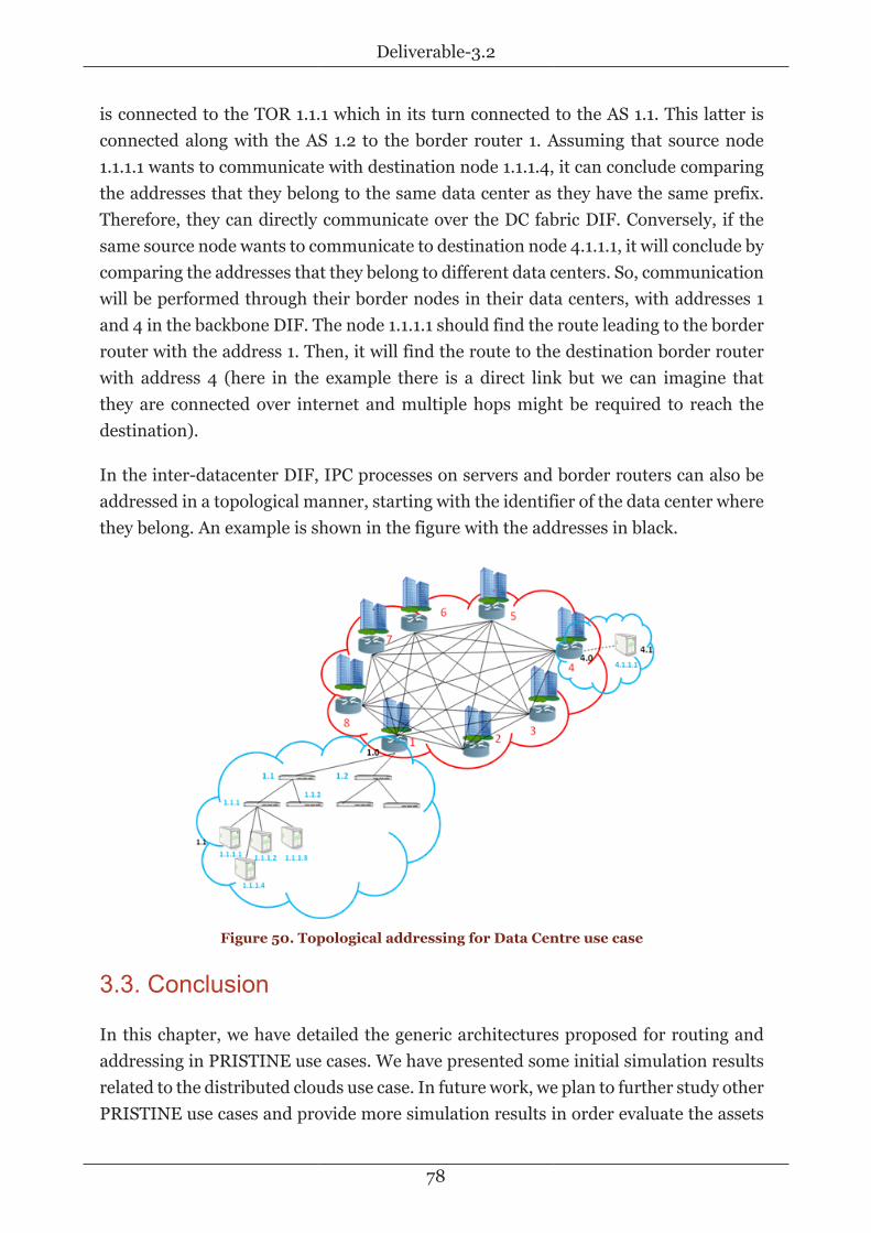
Deliverable-3.2

78

is connected to the TOR 1.1.1 which in its turn connected to the AS 1.1. This latter isconnected along with the AS 1.2 to the border router 1. Assuming that source node1.1.1.1 wants to communicate with destination node 1.1.1.4, it can conclude comparingthe addresses that they belong to the same data center as they have the same prefix.Therefore, they can directly communicate over the DC fabric DIF. Conversely, if thesame source node wants to communicate to destination node 4.1.1.1, it will conclude bycomparing the addresses that they belong to different data centers. So, communicationwill be performed through their border nodes in their data centers, with addresses 1and 4 in the backbone DIF. The node 1.1.1.1 should find the route leading to the borderrouter with the address 1. Then, it will find the route to the destination border routerwith address 4 (here in the example there is a direct link but we can imagine thatthey are connected over internet and multiple hops might be required to reach thedestination).

In the inter-datacenter DIF, IPC processes on servers and border routers can also beaddressed in a topological manner, starting with the identifier of the data center wherethey belong. An example is shown in the figure with the addresses in black.

Figure 50. Topological addressing for Data Centre use case

3.3. Conclusion

In this chapter, we have detailed the generic architectures proposed for routing andaddressing in PRISTINE use cases. We have presented some initial simulation resultsrelated to the distributed clouds use case. In future work, we plan to further study otherPRISTINE use cases and provide more simulation results in order evaluate the assets

Deliverable-3.2

79

of using RINA. Moreover, based on the evaluation results, selected architectures willbe proposed for implementation in the RINA SDK.

Deliverable-3.2

80

List of acronymsACC Aggregate Congestion

Control

AE Application Entity

AI Application Instance

AP Application Process

CACEP Common ApplicationConnection EstablishmentProtocol

CCP Continuity Check Protocol

CDAP Common DistributedApplication Protocol

DA Distributed Application

DAF Distributed ApplicationFacility

DC Data Centre

DIF Distributed IPC Facility

DTCP Data Transfer ControlProtocol

DTP Data Transfer Protocol

E2E End to End

ECN Explicit CongestionNotification

EFCP Error Flow Control Protocol

FA Flow Allocator

FAI Flow Allocator Instance

FIFO First In, First Out

FQ Fair Queuing

IANA Internet Assigned NumbersAuthority

IPC Inter ProcessCommunication

Deliverable-3.2

81

IRM IPC Resource Manager

ISP Internet Service Provider

LAN Local Area Network

LIFO Last In, First Out

MAC Medium Access Control

NM-DMS Network ManagementDistributed ManagementSystem

MPLS Multi-Protocol LabelSwitching

MPLS-TE MPLS with TrafficEngineering extensions

NSM Name-Space Manager

OS Operating System

OSPF Open Shortest Path First

PCI Protocol-Control-Information

PDU Protocol Data Unit

PDUFG PDU Forwarding GeneratorPolicies

PFT Protocol Data UnitForwarding Table

PFTG PDU Forwarding TableGenerator

PoA Point of Attachment

QoS Quality of Service

RA Resource Allocator

RIB Resource Information Base

RINA Recursive InterNetworkArchitecture

RIR Regional Internet Registry

RMT Relaying and MultiplexingTask

Deliverable-3.2

82

RR Round Robin

RSVP-TE ReSerVation Protocolwith Traffic Engineeringextensions

SDU Service Data Unit

SFR Scalable Forwarding inRINA

TCP Transmission ControlProtocol

WLAN Wireless LAN

Deliverable-3.2

83

References• [AlFares] M. Al-Fares, S. Radhakrishnan, B. Raghavan, N. Huang, and A. Vahdat,

“Hedera: Dynamic flow scheduling for data center networks,” in Proc. of USENIXNSDI, San Jose, CA, USA, 2010.

• [Chiesa] Marco Chiesa et al, “Traffic Engineering with Equal-Cost-MultiPath: AnAlgorithmic perspective,” IEEE INFOCOM, 2014.

• [D21] PRISTINE Consortium. Deliverable D2.1. Use cases and requirementsanalysis. May 2014. Available online1 .

• [D22] PRISTINE Consortium. Deliverable D2.2. PRISTINE Reference Framework.June 2014. Available online2 .

• [D61] PRISTINE Consortium. Deliverable D6.1. First iteration trials plan forSystem-level integration and validation. March 2015. Available online3 .

• [Davies] N. Davies, “Delivering predictable quality in saturated networks”,Technical Report, September 2003, available online4

• [EyeQ] EyeQ: Practical Network Performance Isolation at the Edge, imalkumarJeyakumar, Stanford University; Mohammad Alizadeh, Stanford University andInsieme Networks; David Mazières and Balaji Prabhakar, Stanford University;Changhoon Kim and Albert Greenberg, Windows Azure, 10th USENIX Symposiumon Networked Systems and Implementation.

• [Greenberg] A. Greenberg, J. R. Hamilton, N. Jain, S. Kandula, C. Kim, P. Lahiri,D. A. Maltz, P. Patel, and S. Sengupta, “Vl2: A scalable and flexible data centernetwork,” in Proc. of ACM SIGCOMM, Barcelona, Spain, 2009.

• [Guo] C. Guo, H. Wu, K. Tan, L. Shi, Y. Zhang, and S. Lu, “DCell: A Scalable andFault-Tolerant Network Structure for Data Centers,” in Proc. of ACM SIGCOMM,Seattle, WA, USA, 2008.

• [Hopps] C. Hopps, “Analysis of an equal-cost multi-path algorithm,” United States,2000.

• [Niranjan] R. Niranjan Mysore, A. Pamboris, N. Farrington, N. Huang, P. Miri, S.Radhakrishnan, V. Subramanya, and A. Vahdat, “Portland: A scalable fault-tolerant

1 http://ict-pristine.eu/?page_id=372 http://ict-pristine.eu/?page_id=373 http://ict-pristine.eu/?page_id=374 http://www.pnsol.com/public/TP-PNS-2003-09.pdf

Deliverable-3.2

84

layer 2 data center network fabric,” SIGCOMM Comput. Commun. Rev., vol. 39, no.4, pp. 39–50, Aug. 2009. Available online5

• [RFC2991] RFC 2991, “Multipath Issues in Unicast and Multicast Next-HopSelection”, Nov. 2000.

• [Riggio] Roberto Riggio, Francesco De Pellegrini, and Domenico Siracusa, "ThePrice of Virtualization: Performance Isolation in Multi–Tenants Networks", in Proc.of IEEE ManFI 2013.

• [SplitTCP] J. Border, M. Kojo, J. Griner, G. Montenegro, and Z. Shelby,“Performance Enhancing Proxies Intended to Mitigate Link-Related Degradations,”RFC 3135, June 2001.

5 http://doi.acm.org/10.1145/1594977.1592575