deliverable report methodology for active load control · methodology for active load control...
TRANSCRIPT

This project has received funding from the European Union’s Horizon 2020 research and innovation programme under grant agreement No 727477
Closed Loop Wind Farm Control
DELIVERABLE REPORT
Methodology for active load control
Deliverable No. D2.2 Work Package No. WP2 Task/s No. T2.2/T2.3
Work Package Title Wind Farm Flow control technologies and algorithms
Linked Task/s Title Subtask 2.3.1 Wake estimators for partial wake overlap
Subtask 2.2.2/2.2.3 Closed loop wake steering
Subtask 2.3.4 Reliability enhancing technologies
Status Draft Final (Draft/Draft Final/Final)
Dissemination level PU-Public (PU-Public, PP, RE-Restricted, CO-Confidential) (https://www.iprhelpdesk.eu/kb/522-which-are-different-levels-confidentiality)
Due date deliverable 2018-02-28 Submission date 2018-02-28
Deliverable version CL-Windcon_D2.2_DraftFinal_ActiveLoadControl
Ref. Ares(2018)1135492 - 28/02/2018

D2.2 – Methodology for active load control PU-Public
Copyright CL-Windcon Contract No. 727477 Page 2
DOCUMENT CONTRIBUTORS
DOCUMENT HISTORY
Deliverable responsible IK4-IKERLAN
Contributors Organization Reviewers Organization
Inhar Andueza
Iker Elorza
IK4-IKERLAN Alberto Zasso
Alessandro Croce
Stefano Cacciola
Politecnico di Milano
Steffen Raach University of Stuttgart Ursula Smolka Ramboll
Johannes Schreiber
Filippo Campagnolo
Technische Universität München
David Astrain
Irene Eguinoa CENER
Version Date Comment
1.0 2018-02-19 First draft
2.0 2018-02-28 Final draft with corrections after internal review

D2.2 – Methodology for active load control PU-Public
Copyright CL-Windcon Contract No. 727477 Page 3
TABLE OF CONTENTS
1 EXECUTIVE SUMMARY ...........................................................................................................8
2 INTRODUCTION .....................................................................................................................9
3 WAKE ESTIMATORS FOR PARTIAL WAKE OVERLAP DETECTION ............................................. 10
3.1 OBJECTIVES ............................................................................................................................... 10
3.2 CONCEPT OF SECTOR EFFECTIVE WIND SPEED ESTIMATION ................................................... 10
3.3 CONCEPT OF WAKE DETECTION ............................................................................................... 11
3.4 CONCEPT OF WAKE POSITION AND DEFICIT ESTIMATION BY ONLINE MODEL UPDATE ......... 14
3.4.1 Method ................................................................................................................................ 16
3.4.2 Implementation and results ................................................................................................ 17
3.5 CONCLUSIONS .......................................................................................................................... 24
4 EXTERNALLY TRIGGERABLE INDIVIDUAL PITCH CONTROL ...................................................... 26
4.1 INDIVIDUAL PITCH CONTROL .................................................................................................... 26
4.2 OPENDISCON IMPLEMENTATION ............................................................................................. 28
4.3 SIMULATION RESULTS .............................................................................................................. 32
5 CLOSED LOOP WAKE STEERING ............................................................................................. 45
5.1 OBJECTIVES ............................................................................................................................... 45
5.2 GENERAL CONCEPT OF CLOSED-LOOP WAKE STEERING .......................................................... 46
5.2.1 Estimation task .................................................................................................................... 46
5.2.2 Control task ......................................................................................................................... 47
5.3 LIDAR-BASED WAKE TRACKING ................................................................................................ 47
5.3.1 Lidar system......................................................................................................................... 48
5.3.2 Classification of lidar-based wake tracking methods .......................................................... 48
5.3.3 Wake tracking using a Gaussian shape basis function ........................................................ 49
5.3.4 Model-based wake tracking ................................................................................................ 49
5.4 CONTROLLER DESIGN ............................................................................................................... 51
5.4.1 Controller design model ...................................................................................................... 51
5.4.2 Controller design synthesis ................................................................................................. 53
5.4.3 Controller analysis ............................................................................................................... 55
6 RELIABILITY ENHANCING TECHNOLOGIES .............................................................................. 58
6.1 OBJECTIVES ............................................................................................................................... 58
6.2 DESIGN AND IMPLEMENTATION .............................................................................................. 58
6.3 SIMULATION RESULTS .............................................................................................................. 61
7 CONCLUSIONS ..................................................................................................................... 70

D2.2 – Methodology for active load control PU-Public
Copyright CL-Windcon Contract No. 727477 Page 4
8 REFERENCES......................................................................................................................... 71

D2.2 – Methodology for active load control PU-Public
Copyright CL-Windcon Contract No. 727477 Page 5
LIST OF FIGURES
Figure 1. Concept of sector effective wind speed estimation using blade effective wind speed. ........ 11 Figure 2. Sector effective wind speed estimates (SEWS, coloured lines) and reference values from simulation input (black lines). ............................................................................................................... 11 Figure 3. Turbine rotor disc, with two sectors, each of 90 degrees. ..................................................... 12 Figure 4. Wake detection ratio for different ambient wind conditions and turbine yaw angle. .......... 13 Figure 5. Concept of wind farm control with model updating .............................................................. 15 Figure 6. Wind farm layout, top-view. .................................................................................................. 19 Figure 7. Comparison between experimental and modeled turbine power and SE wind speeds. ....... 19 Figure 8. Predictions of the on-line corrected simplistic model (s) compared to experimental measurements (exp). ............................................................................................................................ 21 Figure 9. Downwind turbine power predicted by the wind-sensing method (𝑷𝐖𝐓𝟐,𝐰𝐬), and the power method (𝑷𝐖𝐓𝟐,𝐩), compared with the experimental one (𝑷𝐖𝐓𝟐,𝐞𝐱𝐩), for various modeling errors. .................................................................................................................................... 22 Figure 10. Downwind turbine SE wind speeds predicted by the wind-sensing method 𝑽𝐖𝐓𝟐,𝐰𝐬𝐥𝐞𝐟𝐭/𝐫𝐢𝐠𝐡𝐭and the power method (𝑽𝐖𝐓𝟐,𝐩𝐥𝐞𝐟𝐭/𝐫𝐢𝐠𝐡𝐭), compared to the experimental ones (𝑽𝐖𝐓𝟐,𝐞𝐱𝐩𝐥𝐞𝐟𝐭/𝐫𝐢𝐠𝐡𝐭), for various modeling errors. ...................................................................... 23 Figure 11. Measured wind farm power (𝑷𝐖𝐅,𝐞𝐱𝐩) and model-predicted maximum available wind farm power 𝑷𝐦𝐚𝐱,𝐖𝐅. For t>90s, the experiment reaches the optimal solution.............................. 24 Figure 12. Individual pitch control principle scheme. ........................................................................... 28 Figure 13. Three-dimensional vector reference frame. ........................................................................ 28 Figure 14. Three blade rotating frame of reference. ............................................................................ 29 Figure 15. Externally Triggerable Individual Pitch Control loop. ........................................................... 30 Figure 16. Calculation of the external maximum control actions introduced in the ikConLoop. ......... 31 Figure 17. Two seeds of turbulent wind time histories (above rated region). ..................................... 34 Figure 18. Collective and three blades pitch angles (deg) in above rated region. ................................ 35 Figure 19. Three blades root moments (kN·m) in above rated region. ................................................ 36 Figure 20. My and Mz (kN·m). ............................................................................................................... 37 Figure 21. Pitch y and pitch z (deg). ...................................................................................................... 38 Figure 22. Two seeds of turbulent wind time histories (region transition). ......................................... 39 Figure 23. Collective and three blades pitch angles (deg) in region transition. .................................... 40 Figure 24. Three blades root moments (kN·m) in region transition. .................................................... 41 Figure 25. Blades pitch angle and root moments for uniform wind with extreme wind shear (above rated region). ......................................................................................................................................... 43 Figure 26. Pitch and moments in the non-rotating frame of reference for uniform wind with extreme wind shear (above rated region). .......................................................................................................... 44 Figure 27.The concept of closed-loop wake steering............................................................................ 46 Figure 28. Measurement trajectory of the scanning lidar system facing downwind. .......................... 47 Figure 29. Example of Gaussian basis function fitted to lidar measurement data. The wake position is assumed at the minimum of the fitted function. .................................................................................. 49 Figure 30. The general setup of model-based wind field reconstruction for model-based wake tracking .................................................................................................................................................. 50 Figure 31. An example of the fit of the general model to the lidar measurement data measured in a field testing campaign. .......................................................................................................................... 51 Figure 32. The estimated wake position of different step simulations. ............................................... 52 Figure 33. The different models obtained from the model parametrization.The color order is according to Figure 32. .......................................................................................................................... 53

D2.2 – Methodology for active load control PU-Public
Copyright CL-Windcon Contract No. 727477 Page 6
Figure 34. The bode analysis of the designed 𝑯∞ wake redirection controller. .................................. 55 Figure 35. The performance analysis of the obtained 𝑯∞ controller. ................................................. 56 Figure 36. Time simulations with the nominal controller design model. ............................................. 57 Figure 37. Speed Sensor Manager block. .............................................................................................. 58 Figure 38. Speed Sensor Manager block diagram. ................................................................................ 59 Figure 39. Speed sensors measurements for two turbulent seeds in above rated region. .................. 62 Figure 40. Generator speed equivalent for two turbulent seeds in above rated region. ..................... 63 Figure 41. Sensor measurement zoom in at fault to zero. .................................................................... 64 Figure 42. Sensor measurement zoom in at fault to rated. .................................................................. 65 Figure 43. Speed sensors measurements for two turbulent seeds in below rated region. .................. 66 Figure 44. Generator speed equivalent for two turbulent seeds in below rated region. ..................... 67 Figure 45. Generator electrical torque for two turbulent seeds in below rated region. ...................... 68 Figure 46. Rotor shaft loads, Mxa, for two turbulent seeds in below rated region. ............................. 69
LIST OF TABLES
Table 1. State update implementations. ............................................................................................... 18 Table 2. Diagnoses map ......................................................................................................................... 60

D2.2 – Methodology for active load control PU-Public
Copyright CL-Windcon Contract No. 727477 Page 7
LIST OF ABBREVIATIONS
Abbreviation Description
BE Blade Effective
D Diameter
IPC Individual Pitch Control
SE Sector Effective
SEWS Sector Effective Wind Speed
WT Wind Turbine
CFD Computational Fluid Dynamics
TI Turbulence Intensity

D2.2 – Methodology for active load control PU-Public
Copyright CL-Windcon Contract No. 727477 Page 8
1 EXECUTIVE SUMMARY
As well as power or load management, wind farm control requires specific control mechanisms for
the reduction of loads caused by a wind turbine being a part of a farm. Said loads are mainly due to
partial wake overlap, which forces blades to get in and out of one or more upwind turbine wakes,
with the corresponding increase in fatigue.
CL-Windcon contemplates both the reduction of said cyclic loads via individual pitch control and their
avoidance via wake steering. Individual pitch control requires, however, a considerably increased
pitch actuator activity, which may offset its benefits in terms of blade loads if used continuously.
Something similar may be true about wake steering and the yaw system. It is therefore desirable to
be able to activate or trigger these load-reducing control features only when partial wake overlaps
actually happen. This deliverable presents estimators for partial wake overlap detection, which may
be used for said triggering, as well as a novel closed-loop wake steering methodology. It also presents
the triggerable individual pitch control implemented by OpenDiscon, for its use in WP2 and WP3
simulations.
This deliverable also presents a technique for the management of sensor failure, which is
demonstrated via simulations in which the generator speed measurement is overridden to simulate a
fault. Said technique, which is based on sensor redundancy, may have applications in wind farm
control, where sensor redundancy may not only happen by design, but also by collaboration between
turbines.

D2.2 – Methodology for active load control PU-Public
Copyright CL-Windcon Contract No. 727477 Page 9
2 INTRODUCTION
Large scale Wind Energy penetration requires efficient farm layouts which optimise production and
minimise installation and operating costs. This inevitably results in more and more wind turbines
working in or near the wakes of upwind turbines, as denser and more extensive farm layouts prevail.
A wind turbine working in another’s wake experiences not only a reduction in the wind’s kinetic
energy which is available for extraction, but also a change in the nature of aerodynamic forces it has
to withstand. Said change is typically deleterious, especially when the wake impinges only on a part
of the rotor, because that results in the blades cycling in and out of a lower wind speed region, which
can cause considerable fatigue load.
Given the increasing likelihood of wake impingement and the corresponding ill effects, mitigation
strategies are sought. Individual pitch control (IPC) seems, at face value, especially fitted to the task,
since its primary purpose is to reduce cyclic blade loads due to spatially-varying wind conditions. IPC
can, however, considerably increase the pitch system’s fatigue, even to the point of it becoming
counterproductive to continuously operate a wind turbine with IPC. Another, more novel, option is
to steer the impinging wake away from the turbine, so that the spatially-varying wind conditions are
avoided altogether. This must, of course, be done by yawing the upwind turbine. Doing so in closed
loop may, however, considerably increase the yaw system’s fatigue the same way as IPC can increase
the pitch system’s. It seems therefore advisable to use IPC and/or wake steering only when wake
impingement is expected, thus trading pitch/yaw system fatigue for blade fatigue only when said
trade is advantageous. This requires a method to detect such situations.
Chapter 3 presents wake estimators to detect wake impingement, so that methods such as IPC or
wake steering may then be activated to mitigate the negative effects of said impingement.
Chapter 4 presents the IPC implementation in OpenDiscon, which allows smooth
activation/deactivation during power production and can, therefore, be used in combination with the
estimators in chapter 3.
Chapter 5 presents a novel closed-loop wake steering method. Said method makes it possible to
steer the wake away from a downwind turbine.
Finally, chapter 6 presents a technique for the management of sensor failure, which is demonstrated
via simulations in which the generator speed measurement is overridden to simulate a fault. Said
technique, which is based on sensor redundancy, may have applications in wind farm control, where
sensor redundancy may not only happen by design, but also by collaboration between turbines.

D2.2 – Methodology for active load control PU-Public
Copyright CL-Windcon Contract No. 727477 Page 10
3 WAKE ESTIMATORS FOR PARTIAL WAKE OVERLAP DETECTION
3.1 Objectives
This chapter presents two methods to detect the impingement of a wake on a downstream turbine
using downstream turbine measurements to facilitate wake steering and/or triggered IPC. Both
methods base on an underlying “wind sensing” method, which uses turbine load measurements to
estimate the instantaneous flow field at the given turbine. First, a simple method to detect partial
wake impingement is presented, which could be used to trigger IPC on the turbine and/or trigger the
direction of wake steering at an upstream turbine. Second, a more sophisticated method is described
which additionally utilizes a control oriented wind farm flow model (see Deliverable 1.2) to estimate
wake position and wake deficit of an impinging wake. Such estimates can be a useful feedback for
wake steering and/or wind farm control algorithms as additional wind farm flow information is
provided.
This here reported concepts of “wind sensing” and the simple method to detect partial wake
impingement have mainly been developed previously [1]. The concepts are reported here because
the method to estimate wake position and wake deficit rely on them.
3.2 Concept of sector effective wind speed estimation
It is well known that the turbine response can be used to infer the ambient wind speed by applying a
rotor effective wind speed estimation using the torque or power balance estimation technique [2].
Thereby, the ambient (or rotor effective) wind speed is estimated using the usually known relation
between turbine power coefficient and tip-speed-ratio. However, no information on the localized
flow on the rotor can be obtained.
Here, a method is summarized that uses blade root bending moments and therefore allows the
estimation of the local wind speed at the blade position. Thereby each blade acts as a moving sensor.
Considering a steady wind condition, an out-of-plane coefficient 𝐶𝑚0 is defined as
𝐶𝑚0 𝜆𝐵𝐸 ,𝛽, 𝑞𝐵𝐸 =
𝑚1
2𝜌𝐴𝑅𝑉𝐵𝐸
2, (1)
where 𝜆𝐵𝐸 is the blade effective (BE) tip-speed-ratio, 𝛽 the blade pitch angle, 𝑞𝐵𝐸 the BE dynamic
pressure to take aeroelastic effects into account, 𝑚 the blade out-of-plane bending moment, 𝜌 the
air density, 𝐴 the rotor disc area, 𝑅 the rotor radius and 𝑉𝐵𝐸 the BE wind speed at the blade. The
coefficient can be computed using a turbine simulation model. The coefficient is then used during
turbine operation to solve the given equation with 𝑉𝐵𝐸 as unknown variable giving an estimate of the
BE wind speed.

D2.2 – Methodology for active load control PU-Public
Copyright CL-Windcon Contract No. 727477 Page 11
An estimation of the sector effective (SE) wind speed (defined as the mean ambient wind speed in a
sector of the rotor disc), is obtained by averaging over an azimuthal interval of interest. The estimate
can be updated every time a blade leaves the sector while the zero-order hold can be employed in
between two updates. This concept is symbolically illustrated in Figure 1.
Figure 1. Concept of sector effective wind speed estimation using blade effective wind speed.
As an example, this method is employed on a 3 MW turbine with two sectors (as depicted in Figure
3) on a dynamic simulation using the simulation tool Cp-Lambda [3]. Figure 2 shows estimation
results for a turbulent inflow of intensity 10%, generated with Turbsim [4] the following results can
be obtained:
Figure 2. Sector effective wind speed estimates (SEWS, coloured lines) and reference values from simulation input (black lines).
3.3 Concept of wake detection
There may be multiple ways of detecting a wake impingement by analysing the turbine response.
Here, a simple model-free method to detect partial wake overlap employing the SEWS estimation
method is presented.

D2.2 – Methodology for active load control PU-Public
Copyright CL-Windcon Contract No. 727477 Page 12
Thereto, two sectors can be defined on the rotor disc.
Figure 3. Turbine rotor disc, with two sectors, each of 90 degrees.
By calculating the relative wind speed difference (scaled by the rotor effective wind speed 𝑉𝑅𝐸)
between the two rotor sides δV , a measure of horizontal shear is obtained.
δV =𝑉𝑆𝐸 ,𝑙𝑒𝑓𝑡 − 𝑉𝑆𝐸 ,𝑟𝑖𝑔𝑡
𝑉𝑅𝐸 (2)
In non-waked cases 𝛿𝑉 will be close to zero assuming no significant prevailing ambient horizontal
wind shear. The effect of ambient turbulence, which can lead to horizontal shear measurements has
to be eliminated by low-pass filtering (𝛿𝑉 ) appropriately.
In waked cases, the 𝛿𝑉 will show a positive or negative values depending on the rotor side of wake
impingement. Comparing with a threshold 𝑘 one can distinguish between a left or right sided wake
impingent:
wake impingement = left rotor side, for 𝛿𝑉 > 𝑘
no or full wake, otherwise
right rotor side, for 𝛿𝑉 < 𝑘
(3)
The choice of 𝑘 might depend on the required wake detection sensitivity, expected wake deficit and
ambient turbulence intensity. Clearly, this method does not allow distinguishing between a full wake
impingement and no wake impingement. However, such detection could be obtained by comparing
the estimated sector effective speeds (or rotor effective wind speed/turbine power) to a reverence
value coming from an undisturbed upstream turbine.
As an example, a 3 MW turbine has been simulated with a wake impinging at different lateral
position. Thereto, a turbulent wind field has been obtained by superimposing a Larsen wake model
(EWTSII model) [5] on a turbulent wind grid (Turbsim). The chosen threshold 𝑘 was set to 0.12.

D2.2 – Methodology for active load control PU-Public
Copyright CL-Windcon Contract No. 727477 Page 13
Figure 4 summarizes results of the wake detector at ambient wind speed of 8m/s. Each subplot has a
different combination of turbulence intensity (TI) and turbine yaw misalignment (𝛾) showing the
robustness of the method. For different overlaps, each plot displays the detection ratio on the right
sector (dark blue bars pointing upwards), and on the left one (light blue bars pointing downwards).
The detection ratio is defined as the ratio of the number of time instants when the wake is detected,
divided by the total number of time instant in a sequence of a given length (here chosen to be
10 min). For the nominal case (TI=5%, 𝛾=0°) the detection ratio is 1 for wake overlaps of ±0.25D up
to ±0.75D. At higher turbulence intensity (TI=10%, 𝛾=0°) the detection ratios do not
reach 1 anymore, as the wake deficit is less strong. However, it is important to note that also no false
positives at a lateral position of the wake center of ±1.25D are detected. In case the wake detecting
turbine itself tries to deflect its own wake, it might operate with significant yaw misalignment.
Therefore two cases are shown in which the turbine is misaligned by 𝛾=±20°. Such yaw misalignment
has an effect on turbine loads and might therefore disturb the sector effective wind speed estimation
used for wake detection. Nevertheless very high detection ratios are obtained and no false positives
can occur.
TI=5%, 𝛾=0°
TI=10%, 𝛾=0°
TI=5%, 𝛾=-20°
TI=5%, 𝛾=-20°
Figure 4. Wake detection ratio for different ambient wind conditions and turbine yaw angle.

D2.2 – Methodology for active load control PU-Public
Copyright CL-Windcon Contract No. 727477 Page 14
3.4 Concept of wake position and deficit estimation by online model update
In addition to the binary wake detector described in Chapter 3.3, a more sophisticated method is
described in this chapter. The method utilizes again the sector effective wind speed estimator, but
evaluates the estimates by comparing them to a control oriented wind farm flow model (see
Deliverable 1.2, Chapter 6 – FLORIS). Thereby, it is possible to estimate the wake position as long as
the wake is impinging on a downstream turbine rotor. In case of a relatively full wake impingement,
which leads to wind speed changes in both sectors of the downstream turbine, it is also possible to
estimate the wake speed. Further turbine measurements, i.e. turbine power or rotor effective wind
speed, that are usually also modelled in a control oriented wind farm model can also additionally
improve the wake estimation.
The wake estimator could be used to trigger IPC on downstream turbines or as feedback for wake
steering and/or wind farm control algorithms. Here, the concept of wake estimation is described for
the application in a wind farm control algorithm. Therefore, the wake estimation is directly linked to
the updated wake deficit and wake position in the wind farm model. The following work has also
been submitted for publication in [6].
Each turbine in a wind farm emits a wake characterized by reduced velocity and increased
turbulence, leading to losses in power production and increased loads on downwind turbines. The
negative effects of wake interactions may be mitigated by wake management strategies [7]. One
possible implementation of such strategies is based on a wind farm flow model: the predictions of
the model are used by a controller, whose aim is to energize and/or redirect wakes for improved
energy yield and/or reduced loading.
However, the performance of any such model-based control method is inherently limited by the
accuracy of the model it is based upon in predicting the behaviour of shed wakes. Unfortunately, any
model is wrong –at least in some situations–, especially the simple reduced-order or engineering
models used for control synthesis. The only way to improve at run time the fidelity of a model is to
correct its predictions on the basis of measurements made on the plant. Figure 5 illustrates this
concept.
D2.2 – Methodology for active load control PU-Public
Copyright CL-Windcon Contract No. 727477 Page 15
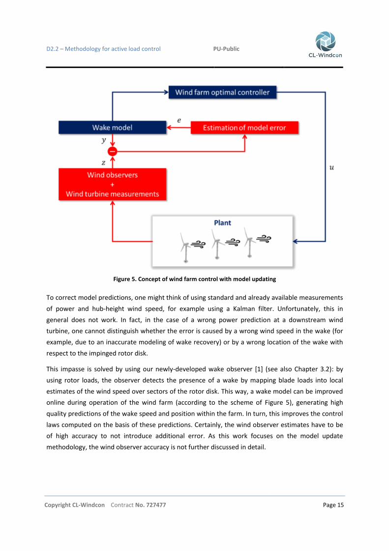
Figure 5. Concept of wind farm control with model updating
To correct model predictions, one might think of using standard and already available measurements
of power and hub-height wind speed, for example using a Kalman filter. Unfortunately, this in
general does not work. In fact, in the case of a wrong power prediction at a downstream wind
turbine, one cannot distinguish whether the error is caused by a wrong wind speed in the wake (for
example, due to an inaccurate modeling of wake recovery) or by a wrong location of the wake with
respect to the impinged rotor disk.
This impasse is solved by using our newly-developed wake observer [1] (see also Chapter 3.2): by
using rotor loads, the observer detects the presence of a wake by mapping blade loads into local
estimates of the wind speed over sectors of the rotor disk. This way, a wake model can be improved
online during operation of the wind farm (according to the scheme of Figure 5), generating high
quality predictions of the wake speed and position within the farm. In turn, this improves the control
laws computed on the basis of these predictions. Certainly, the wind observer estimates have to be
of high accuracy to not introduce additional error. As this work focuses on the model update
methodology, the wind observer accuracy is not further discussed in detail.

D2.2 – Methodology for active load control PU-Public
Copyright CL-Windcon Contract No. 727477 Page 16
Section 3.4 is organized as follows. Section 3.4.1 formulates the model update approach, the wind
farm model and the load-based wind observer. Section 3.4.2 describes different possible
implementations of the model-update method. The various options are then tested with reference to
experimental measurements obtained on a scaled wind farm facility operated in a large boundary
layer wind tunnel. Finally, Section 3.5 summarizes results and conclusions, and gives an outlook
towards future work.
3.4.1 Method
State update
The model update method is formulated here based on a generic non-linear static wind farm model.
A similar formulation could also be derived for a dynamic model, leading to a standard Kalman
filtering problem. The static model is written as
𝑥 = 𝑓 𝑢,𝑚,𝑝 (4)
𝑦 = 𝑔 𝑥 (5)
where 𝑓 is a non-linear static function. The control inputs are noted 𝑢, and include the yaw and
induction of each wind turbine in the farm. Measurements of ambient conditions are noted 𝑚, and
include density and free stream wind speed and direction (typically estimated by the upstream wind
turbines). Physical tunable coefficients of the model and the wind farm layout are captured by the
vector of parameters 𝑝. The model states are indicated as 𝑥, here they include the velocity and
position of the wake of each turbine. A set of outputs 𝑦 is defined by function 𝑔. The outputs include
the estimated sector effective flow velocities at the downstream rotors.
In general, the predictions of the model states will be in error, due to a lack of model fidelity,
mistuning of the parameters or inaccuracies in ambient conditions. This can be corrected by
introducing a state error 𝑒. The corresponding corrected state 𝑥 becomes
𝑥 = 𝑥 + 𝑒. (6)
A maximum likelihood estimate of the state error can be readily obtained by solving the following
problem
min𝑒
𝑧 − 𝑦 T𝑅−1 𝑧 − 𝑦 , (7)
where 𝑧 are measurements and 𝑦 the corresponding updated model outputs (𝑦 = 𝑔 𝑥 ). For a given
fixed measurement error covariance 𝑅, this procedure corresponds to a standard weighted least
squares.

D2.2 – Methodology for active load control PU-Public
Copyright CL-Windcon Contract No. 727477 Page 17
Note that, as ambient wind conditions are often uncertain, the presented formulation could be
extended by including them within the list of states. However, it is also clearly necessary to ensure
the observability of all chosen states. For example, a wrong wind direction might not be
distinguishable from a wrong wake location. The development of a general formulation for the
estimation of wind farm flow model states is a problem of great interest, which is however outside of
the scope of the present work.
Wind farm model
The wind farm model (see Deliverable 1.2) includes two components: a wake model and a power
model. The wake model is based on the double Gaussian profile proposed by [8], combined with the
yaw-induced wake deflection developed in [9]. The combination of the two models gives the
evolution of the flow speed within the wake downstream of each rotor disk, together with its spatial
location. The power model translates the flow speed into turbine power by computing the mean flow
speed at the turbine rotors using a disk-attached grid. The power coefficient is assumed to be
constant below rated wind speed, and it is corrected to take into account turbine yaw misalignment
with respect to the incoming wind direction.
When implementing the state update for wake speed 𝑢, Eq. (6) is modified as 𝑢 = 𝑢 + 𝑟𝑒, where 𝑟 is
the wake reduction. Since some wake models (i.e. those that base on a Gaussian wake shape) do not
have a well defined wake width, this form of the error avoids changing the ambient wind speed away
from the wake.
Wind observer
A load-based wind speed observer [1] (see also Chapter 3.2) is used to estimate the flow at the
downstream wind turbine. The observer works by mapping blade loads into local estimates of the
wind speed. These are then averaged over sectors of the rotor disk. The resulting sector-effective
(SE) wind speed measurements on the left and right parts of the rotor (noted 𝑉SE ,left and 𝑉SE ,right ,
respectively) are then used in the state update formulation described earlier on.
3.4.2 Implementation and results
Implementation
To evaluate the proposed method, three versions of the state update formulation are implemented
for a simple wind farm consisting of two wind turbines. In the notation used below, the upstream
wind turbine is indicated as WT1, while the downstream one as WT2.

D2.2 – Methodology for active load control PU-Public
Copyright CL-Windcon Contract No. 727477 Page 18
The simplistic method (subscript 𝑠) is intended to demonstrate that, by only using power
measurements at the downwind turbine (𝑃WT 2,exp ), it is in general not possible to correct at the
same time for errors in lateral wake position (𝑑WT 1) and speed (𝑢WT 1) of the upstream wind turbine.
In contrast to the simplistic method, the power method (subscript 𝑝) is well-posed, as it only tries to
correct the wake speed and not its position based on downstream power measurements. The wind-
sensing method (subscript 𝑤𝑠) includes as measurements also the SE wind speeds obtained by the
wind observer on the downwind turbine 𝑉WT 2,expSE ,left /right
. This way, the method is able to correct for
both speed and position in the wake.
Table 1 gives an overview of the three different approaches. For all cases, the ambient conditions are
obtained from the front wind turbine: wind direction is measured by the on-board wind vane, while
the ambient wind speed is computed by the rotor effective wind speed corrected for yaw
misalignment.
Method: Simplistic (∗= 𝑠) Power (∗= 𝑝) Wind-sensing (∗= 𝑤𝑠)
𝑥(∗) = 𝑑WT 1
𝑢WT 1 𝑢WT 1
𝑑WT 1
𝑢WT 1
𝑥 (∗) = 𝑑WT 1 + 𝑒d
𝑢WT 1 + 𝑟𝑒u 𝑢WT 1 + 𝑟𝑒u
𝑑WT 1 + 𝑒d
𝑢WT 1 + 𝑟𝑒u
𝑦 (∗) = 𝑃WT 2 𝑃WT 2
𝑃WT 2
𝑉WT 2SE ,right
𝑉WT 2SE ,left
𝑧(∗) = 𝑃WT 2,exp 𝑃WT 2,exp
𝑃WT 2,exp
𝑉WT 2,expSE ,right
𝑉WT 2,expSE ,left
Table 1. State update implementations.
Experimental setup
Experimental tests with scaled wind turbine models were used to study the performance of the
various state update formulations. The scaled turbines, designed for realistic wake behavior, were
operated in the boundary layer wind tunnel of the Politecnico di Milano at an ambient hub-height
wind speed of 5.8 m/sec and a turbulence intensity of about 5%. A detailed description of the
turbines and the wind tunnel can be found in [10][11]. The wind farm layout is depicted in Figure 6.
Wind farm layout, top-view. The two turbines are operated at a longitudinal distance of 4 diameters
(D) with no lateral displacement.

D2.2 – Methodology for active load control PU-Public
Copyright CL-Windcon Contract No. 727477 Page 19
Figure 6. Wind farm layout, top-view.
The wind farm model parameters 𝑝 were first manually tuned with the objective of obtaining a good
fit of the model predictions with the experimentally measured wake speed, downstream turbine
power and SE speeds at various yaw misalignments of WT1 (𝛾WT 1). Figure 7 shows in the upper
subplot a comparison between measured (subscript 𝑒𝑥𝑝) and modeled power at both turbines. The
lower subplot shows the SE wind speeds for the left and right sectors of WT2. As the G1 models used
in the experiments are not equipped with blade load sensors, blade loads were reconstructed as
described in [11]. To account for the fact that the experimental reconstructed blade loads do not
contain frequencies above 1P (one per revolution), also the SE wind speed obtained from the wind
farm model was filtered by best fitting a linear wind field over the turbine rotor disk. Each
experimental data point represents the mean value of a 60 sec time recording.
Figure 7. Comparison between experimental and modeled turbine power and SE wind speeds.

D2.2 – Methodology for active load control PU-Public
Copyright CL-Windcon Contract No. 727477 Page 20
Results
An experimental time sequence was obtained by stacking one after the other a number of
recordings, each one corresponding to a different constant yaw setting of the front machine. Since
the flow is turbulent, wake dynamics induced by turbulent fluctuations, including meandering, are
included in the recordings. However, the effects of transient changes from one yaw set point to the
next are not, including the corresponding travel-time wake delays, which can be estimated to be
approximatively equal to 1 sec. In any case, such delays are not included in a static model as the one
used here and, on account of this, all signals were filtered with a moving average of 4 sec.
Figure 8 shows the performance of the simplistic state update method. The upper subplot shows the
time history of the upwind turbine yaw position (𝛾WT 1), which changes in three steps from 0 deg to
30 deg. The last yaw position is the approximate point of maximum power production for the present
wind farm configuration. The second subplot shows the experimentally measured power produced
by the downwind turbine (𝑃WT 2,exp ), together with the state updated model prediction (noted
𝑃WT 2,s, where the second subscript indicates the simplistic formulation). The two lines are essentially
identical, indicating an almost perfect prediction of power output by the model. The plot also shows
that power increases after each yaw step, which is indeed caused by the wake deflecting laterally and
thereby reducing its effects on the downstream rotor.
The third subplot shows the SE wind speeds in the left and right turbine sectors. The experimental
measurements from the wind speed observer (solid lines) show the direction of wake deflection:
with increasing time and yaw, the flow velocity in the left sector increases, implying that the wake
center is moving to the right. The SE wind speeds of the updated simplistic method are also shown
on the same plot using dotted lines. These curves reveal that the model-predicted flow velocities,
which were not explicitly taken into account by the method, behave in a radically different way from
the measured ones. In fact, the simplistic state update method corrects the wake center position by
moving it to the left of the downwind turbine, instead of to the right as it should be. The last subplot
of Figure 8 shows the corresponding state errors. The large error in wake speed significantly alters
the wake deficit, while the error in wake position implies that the wake center is located to the left of
the rotor.
The simplistic method is clearly ill-posed, as two states are corrected using only one measurement.
Therefore, multiple combinations of wake speed and displacement can be obtained that, although
completely wrong, still apparently lead to a very good power estimate. A controller using the
predictions of such a model is invariably bound to fail.

D2.2 – Methodology for active load control PU-Public
Copyright CL-Windcon Contract No. 727477 Page 21
Notice that the ill-posedness of the present formulation is rather obvious, by considering that one
single global rotor measurement as power cannot distinguish between changes due to a different
wake recovery or position. This might not be so obvious when using a more complex farm flow
model, as for example a CFD-based approach. However, even in that case, we believe that the
problem of ill-posedness would still be present, and might lead to wrong corrections and hence
wrong flow predictions.
Figure 8. Predictions of the on-line corrected simplistic model (s) compared to experimental measurements (exp).
D2.2 – Methodology for active load control PU-Public
Copyright CL-Windcon Contract No. 727477 Page 22
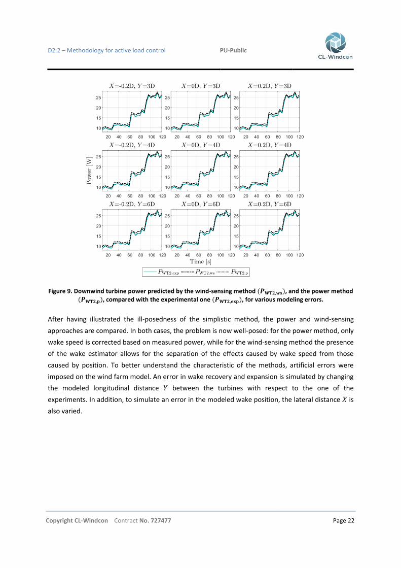
Figure 9. Downwind turbine power predicted by the wind-sensing method (𝑷𝐖𝐓𝟐,𝐰𝐬), and the power method
(𝑷𝐖𝐓𝟐,𝐩), compared with the experimental one (𝑷𝐖𝐓𝟐,𝐞𝐱𝐩), for various modeling errors.
After having illustrated the ill-posedness of the simplistic method, the power and wind-sensing
approaches are compared. In both cases, the problem is now well-posed: for the power method, only
wake speed is corrected based on measured power, while for the wind-sensing method the presence
of the wake estimator allows for the separation of the effects caused by wake speed from those
caused by position. To better understand the characteristic of the methods, artificial errors were
imposed on the wind farm model. An error in wake recovery and expansion is simulated by changing
the modeled longitudinal distance 𝑌 between the turbines with respect to the one of the
experiments. In addition, to simulate an error in the modeled wake position, the lateral distance 𝑋 is
also varied.

D2.2 – Methodology for active load control PU-Public
Copyright CL-Windcon Contract No. 727477 Page 23
For nine combinations of modeling errors, Figure 9 reports the model-predicted power together with
the experimentally measured one. Independently of the modeling error, it appears that power is
always well predicted. The SE wind speeds at the downwind turbine are shown in Figure 10. Solid
lines represent experimental measurements, dotted lines the power method and dash-dotted lines
the wind-sensing method flow speeds. The wind-sensing method provides predictions that are very
close to the experimental measurements, independently of the modeling error. In fact, both wake
speed and wake position can be corrected independently by this approach. On the other hand, the
power method only corrects wake speed. Therefore, it provides good results only in the case of
model errors in the longitudinal displacement (middle column of the subplots). However, as soon as
there is also an error in the wake position, flow velocities do not match anymore. These
discrepancies may translate into significant deficiencies when it comes to utilize the wind farm model
for control purposes.
Figure 10. Downwind turbine SE wind speeds predicted by the wind-sensing method 𝑽𝐖𝐓𝟐,𝐰𝐬𝐥𝐞𝐟𝐭/𝐫𝐢𝐠𝐡𝐭
and the power
method (𝑽𝐖𝐓𝟐,𝐩𝐥𝐞𝐟𝐭/𝐫𝐢𝐠𝐡𝐭
), compared to the experimental ones (𝑽𝐖𝐓𝟐,𝐞𝐱𝐩𝐥𝐞𝐟𝐭/𝐫𝐢𝐠𝐡𝐭
), for various modeling errors.

D2.2 – Methodology for active load control PU-Public
Copyright CL-Windcon Contract No. 727477 Page 24
To illustrate this point, Figure 11 shows for one of the nine cases considered above the maximum
possible wind farm power predicted by the model by yawing the upwind turbine to its optimal
position. In the experiment, the optimal position is approximatively equal to 30 deg, which are
reached after 90 sec. Even though the power method is apparently able to match the downwind
turbine power during the experiment, this is in reality based on a wrong prediction of the flow within
the farm. Hence, the maximum predicted power is highly overestimated. On the other hand, the
wind-sensing method, being capable of a more faithful prediction of the actual flow, provides a
realistic estimate on the maximum achievable power throughout the whole test case. This proves the
importance of correctly modeling the flow within the wind farm for control purposes.
Figure 11. Measured wind farm power (𝑷𝐖𝐅,𝐞𝐱𝐩) and model-predicted maximum available wind farm power
𝑷𝐦𝐚𝐱,𝐖𝐅. For t>90s, the experiment reaches the optimal solution.
3.5 Conclusions
A model-based wind farm control algorithm can only be as good as its underlying model. In a realistic
scenario, various sources of uncertainties and model defects limit the predictive capabilities of any
wind farm flow model. After having calibrated the model offline, the only remaining way to improve
this situation is to correct the predictions of the model online, by using measurements obtained on
the plant.
In this chapter first a method to estimate the flow speed in different sectors of a wind turbine rotor
has been described. The methods utilizes blade root bending moments are becoming more and more
available in modern turbines, especially in those equipped with IPC. For those turbines, the method
would not require additional hardware and could be implemented by a software upgrade.
In Chapter 3.3 a method is presented that processes the difference in sector effective wind speed
estimates on a rotor, to detect an impinging wake. The method is relatively simple and does not
require wake models. As a drawback it is only possible to detect the rotor side of wake impingement
and tuning of the wake detection threshold parameter might has to be scheduled with ambient wind
conditions.

D2.2 – Methodology for active load control PU-Public
Copyright CL-Windcon Contract No. 727477 Page 25
Chapter 3.4 a model based method for wake detection is presented in the framework of an online
wind farm model update method. Therein the sector effective wind speed, estimated by the
individual turbine is used to correct the wake location and deficit predicted by the wake model. This
updated model is believed to provide accurate information on wake position and deficit within the
wind farm.
The developed method can provide valuable information of wake position and reduction. Such
information is believed to be of high importance for wind farm control applications. The information
on wake position might also be of interest regarding triggered IPC (see Chapter 4). However, it is still
unclear whether such implementation can provide any benefit compared to an IPC triggering by
turbine loads directly.
The present work is to be considered only as a preliminary study, and further investigations are
planned. These include studies of observability in the case of only partially impinging wakes, as well
as the investigation of more complex wake interference scenarios. The model-update formulation
will also be exploited for designing wind farm control laws using optimal model-based approaches
(Delivery 3.6).

D2.2 – Methodology for active load control PU-Public
Copyright CL-Windcon Contract No. 727477 Page 26
4 EXTERNALLY TRIGGERABLE INDIVIDUAL PITCH CONTROL
4.1 Individual pitch control
Individual pitch control, as can be noted by its name, consists on controlling the pitch angle of each
blade individually. Wind turbulences and shear cause cyclic loads in very large turbines resulting in
high fatigue damages. The huge area encompassed by the turbine blades and the irregular behaviour
of wind implies considerable differences on wind speed all along the surface covered by the rotor,
especially going up in height. Combined with the rotation of the turbine, blades suffer different loads
depending on its position. Due to that, periodically changing loads are obtained in the blades.
Controlling each blade pitch angle individually makes possible a considerable reduction of these
loads.
Standard turbine models typically include the dynamics of the fixed and rotating turbine components
and are thus time varying in nature owing to the changing angular orientation of the rotating blades.
Application of the Coleman transformation to the inputs and the inverse Coleman transformation to
the outputs of the rotational system, relating blade-pitch angles to blade root bending moments,
gives rise to a transformed system defined in a fixed coordinate frame. Such a system is time
invariant and hencemore amenable to standard feedback control design techniques.
The Coleman transform uses the averaged blade-pitch demand 𝛽 (𝑡), along with the tilt and yaw
referred pitch angles, 𝛽𝑡𝑖𝑙𝑡 (𝑡) and 𝛽𝑦𝑎𝑤 (𝑡), respectively, to yield the total pitch angle demands on
each blade, 𝛽 1,2,3(𝑡), according to the following expression:
𝛽1(𝑡)𝛽2(𝑡)𝛽3(𝑡)
=
1 cos𝜃(𝑡) sin𝜃(𝑡)
1 cos(𝜃 𝑡 +2𝜋
3) sin(𝜃 𝑡 +
2𝜋
3)
1 cos(𝜃 𝑡 +4𝜋
3) sin(𝜃 𝑡 +
4𝜋
3)
𝛽 (𝑡)𝛽𝑡𝑖𝑙𝑡 (𝑡)
𝛽𝑦𝑎𝑤 (𝑡) (8)
where 𝜃 𝑡 is the rotor azimuth angle. The relevant outputs of the turbine are the total blade root
flap-wise bending moments, 𝑀1,2,3(𝑡), that are related to the tilt and yaw moments, 𝑀𝑡𝑖𝑙𝑡 (𝑡) and
𝑀𝑦𝑎𝑤 (𝑡)via the inverse Coleman transform:
𝑀 (𝑡)𝑀𝑡𝑖𝑙𝑡 (𝑡)
𝑀𝑦𝑎𝑤 (𝑡) =
1
3
1
3
1
32
3cos𝜃(𝑡)
2
3cos(𝜃 𝑡 +
2𝜋
3)
2
3cos(𝜃 𝑡 +
4𝜋
3)
2
3sin𝜃(𝑡)
2
3sin(𝜃 𝑡 +
2𝜋
3)
2
3sin(𝜃 𝑡 +
4𝜋
3)
𝑀1(𝑡)𝑀2(𝑡)𝑀3(𝑡)
(9)

D2.2 – Methodology for active load control PU-Public
Copyright CL-Windcon Contract No. 727477 Page 27
The averaged flap-wise blade bending moment is 𝑀 (𝑡) and has a physical interpretation in terms of
the hub loading but is not commonly considered in IPC schemes. Linearization removes explicit
dependence of the turbine model upon the averaged quantities 𝛽 (𝑡) and 𝑀 (𝑡), and so attention
needs only be paid to the tilt and yaw signals in the fixed reference frame. The Coleman relationships
of relevance to the IPC are defined as follows:
𝛽1(𝑡)𝛽2(𝑡)𝛽3(𝑡)
=
cos𝜃(𝑡) sin𝜃(𝑡)
cos(𝜃 𝑡 +2𝜋
3) sin(𝜃 𝑡 +
2𝜋
3)
cos(𝜃 𝑡 +4𝜋
3) sin(𝜃 𝑡 +
4𝜋
3)
𝛽𝑡𝑖𝑙𝑡 (𝑡)
𝛽𝑦𝑎𝑤 (𝑡) (10)
the inverse transformation:
𝑀𝑡𝑖𝑙𝑡 (𝑡)
𝑀𝑦𝑎𝑤 (𝑡) =
2
3 cos𝜃(𝑡) cos(𝜃 𝑡 +
2𝜋
3) cos(𝜃 𝑡 +
4𝜋
3)
sin𝜃(𝑡) sin(𝜃 𝑡 +2𝜋
3) sin(𝜃 𝑡 +
4𝜋
3)
𝑀1(𝑡)𝑀2(𝑡)𝑀3(𝑡)
(11)
The most common approach in the wind turbine individual pitch control relies on a transformation
between frames of reference as described in [12]. This approach was originally introduced by Park
[13] and has been successfully used for vector control of electric machines. It is perfectly fitted for
the wind turbine application since the transfer of the loading from the blades to the fixed structure is
in fact a physical transformation between the rotational and the fixed frame of reference.
Figure 12 displays a basic individual pitch control loop. Measured blade loads and rotor azimuth are
entered as inputs. Blade loads are measured in the rotational blade frame of reference. They are
transformed into the fixed frame of reference using the Park transformation. This transformation
results in the loads on the fixed part of the wind turbine structure in two main axes - y and z that are
usually referred to as tilt and yaw loads. Park’s transformation also produces a zero-sequence
component that accounts for mean values. Such a component is not of interest for load reducing
controller so it is usually omitted in individual pitch control applications.
The control algorithm processes variables, My and Mz, from the fixed frame of reference. Regular
individual pitch control consists of two PI controllers, for moments around axes y and z, respectively.
Its algorithm calculates the appropriate pitch angles y and z for load reduction basing on the
inputted moment values. Outputted variables are in the fixed frame of reference. Using Park’s
inverse transformation pitch angles are transformed into rotational blade frame of reference. These
new variables are the pitch differentials for each blade. To control the rotor speed while reducing
loads in blades, pitch differentials are added to the collective pitch angle [12][15].

D2.2 – Methodology for active load control PU-Public
Copyright CL-Windcon Contract No. 727477 Page 28
Figure 12. Individual pitch control principle scheme.
4.2 OpenDiscon implementation
The control loop implemented by OpenWitcon, ikIpc, for the individual pitch control is showed in
Figure 15. It is based in the same principle as the previous scheme, but instead of using Park’s
transformation, file ikVector has been implemented to transform frame of reference from rotating to
non-rotating. ikVector represents three-dimensional vectors. Blade root moments are expressed in
coordinates of the corresponding rotating frames of reference as defined in ikIpc. This is an array of 3
instances of ikVector, each with 3 coordinates. The coordinates in the first ikVector correspond to
blade 1 root moments around local axes x', y' and z', in that order. The second and third instances of
ikVector have the homologous information regarding blades 2 and 3, respectively.
The non-rotating frame of reference is defined by axes x, y and z. x points downwind, z points up and
y complies with the right hand rule. The rotating frame of reference local to blade 1 is defined by
axes x′, y′ and z′. x′ points downwind, z′ points from the blade root to the blade tip and y′ complies
with the right hand rule. Therefore, as shown in Figure 13, axes x and x′ coincide, and the rotating
frame of reference rotates around them.
Figure 13. Three-dimensional vector reference frame.

D2.2 – Methodology for active load control PU-Public
Copyright CL-Windcon Contract No. 727477 Page 29
The rotating frames of reference local to blades 2 and 3 are defined by axes {x′′,y′′,z′′} and
{x′′′,y′′′,z′′′}, respectively. x′′ and x′′′ also coincide with x, z′′ and z′′′ also point from their respective
blade roots to their respective blade tips, and y′′ and y′′′ also comply with the right hand rule. The
three rotating frames of reference local to blades 1, 2 and 3, respectively, rotate in unison, and are
permanently 120º from each other, as shown in Figure 14. Note that two arrangements are possible.
To accommodate different turbine-specific idiosyncrasies, the azimuth angle θ is defined as the
positive rotation around x necessary to bring z to coincide with z′, minus constant angle φ, which
may be specified via ikIpc_init. Similarly, the position of blades 2 and 3 relative to that of blade 1 is
defined by parameter s, as shown below. s may also be specified via ikIpc_init. In the struct ikIpc_init
individual pitch control initialization parameters are defined, where angle φ corresponds to the
azimuth offset, with a default value of 0.0, and s to the blade order, with a default value of 1. Also
My and Mz control parameters are initialized there.
Figure 14. Three blade rotating frame of reference.
Measured moments My and Mz, along with the demanded values for them and the maximum
control actions for pitches y and z are the inputs of the ikConLoop block, which is described in the
Deliverable 2.1. There are two ikConLoop blocks, as shown in Figure 15. To calculate the control
value for pitch z, measured and demanded My are used as reference and it is limited by maximum
pitch z, which is calculated externally with the loop of Figure 16. Whilst to calculate the control value
for pitch y, the inputs are measured and demanded Mz and it is limited by maximum pitch y.

D2.2 – Methodology for active load control PU-Public
Copyright CL-Windcon Contract No. 727477 Page 30
The outputted pitch angles are contrasted with their corresponding external pitches. The differences
between angles from control and external angles are the pitches around axes y and z. Then they are
transformed from fixed to rotating frame of reference, obtaining the pitch differential for each blade.
The differential on each individual pitch angle is the necessary change on pitch for each blade to
meet the demanded moments. These differences are applied to the collective pitch angle which is
used to control the rotor speed.
Figure 15. Externally Triggerable Individual Pitch Control loop.

D2.2 – Methodology for active load control PU-Public
Copyright CL-Windcon Contract No. 727477 Page 31
In Figure 16 it can be observed the block diagram for the calculation of maximum pitch limits that are
introduced in ikConLoop. First, the collective pitch angle is subtracted to maximum and minimum
pitch angles. The result of the maximum pitch is compared with zero, choosing the minimum value.
The same is done with the minimum pitch result, but in this case the maximum value is selected. The
absolute values of both resultant variables are compared once again to pick out the least. This value
is contrasted one last time with the maximum individual pitch. The smallest one is used as the
maximum pitch increment module along with pitch angles y and z from control, outputted by the
ikConLoop controller. With the maximum pitch increment module and values of pitches y and z from
controller in Figure 15, maximum angles for pitch y and pitch z are calculated. For that the
Pythagorean Theorem is used, where maximum pitches and pitches from control are the legs and
maximum pitch increment module is the hypotenuse. Maximum pitch y is calculated using pitch z
from control and maximum pitch z is calculated using pitch y from control.
To activate the individual pitch control the variable maximum individual pitch must have a value
higher than zero. The value of the maximum individual pitch is used to calculate the maximum pitch
limits for pitch y and pitch z. If the value of the maximum individual pitch is zero, the value of the
maximum pitch increment module would be zero, and consequently, the maximum limits for pitch y
and z. Then, external maximum control actions entered in the ikConLoop blocks would be zero. There
would not be any differential in the individual pitch angles so a collective pitch angle would be
maintained.
Figure 16. Calculation of the external maximum control actions introduced in the ikConLoop.

D2.2 – Methodology for active load control PU-Public
Copyright CL-Windcon Contract No. 727477 Page 32
4.3 Simulation results
To test the individual pitch control the value of maximum individual pitch is changed to non-zero. A
triggering file has been implemented in the control, which activates the IPC during the simulation
and then deactivates it again setting maximum individual pitch to zero, so the effect of the IPC can be
easily studied. The IPC is triggered at the 30th second of the simulation that is when the value of the
maximum individual pitch is set to 10. It is held activated for 30 seconds ending in the 60th. In the 25th
second the value of the maximum individual pitch starts decreasing in a ramp until its deactivation.
For the test, a ramp of 5 seconds with pitch rate of 2 degrees per second has been set to avoid too
fast changes that can derive in loads.
Although for the analysis of the IPC a triggering file has been added to OpenWitcon, the way that
ikIpc is implemented facilitates its external activation. For that the parameter
con.in.maximumIndividualPitch must be modified to the desired maximum individual pitch value. In
this case, the triggering file implemented is called with a function, ikMaximumIndividualPitch, where
the time variable is inputted and a different value of maximum individual pitch is outputted
accordingly. This is a pretty simple testing file that has been implemented for the study, but it serves
as example of how an external trigger can be implemented. Changing the parameter externally with
a variable from Simulink, a load or wake detection system or the supercontroller would be simple
then.
For the simulations above rated wind speeds have been used. Individual pitch control only activates
when the turbine is operating at full load in the 3rd region and it is controlled with the pitch angle.
Due to that, based on design load case 1.2, six seeds of wind speeds from rated to cut-out have been
simulated using a normal turbulence model. Simulation time has been shortened, from the 600
seconds required by the rule, to 100 seconds. This has been considered enough to study the effects
of the IPC in the 30 seconds it is activated.
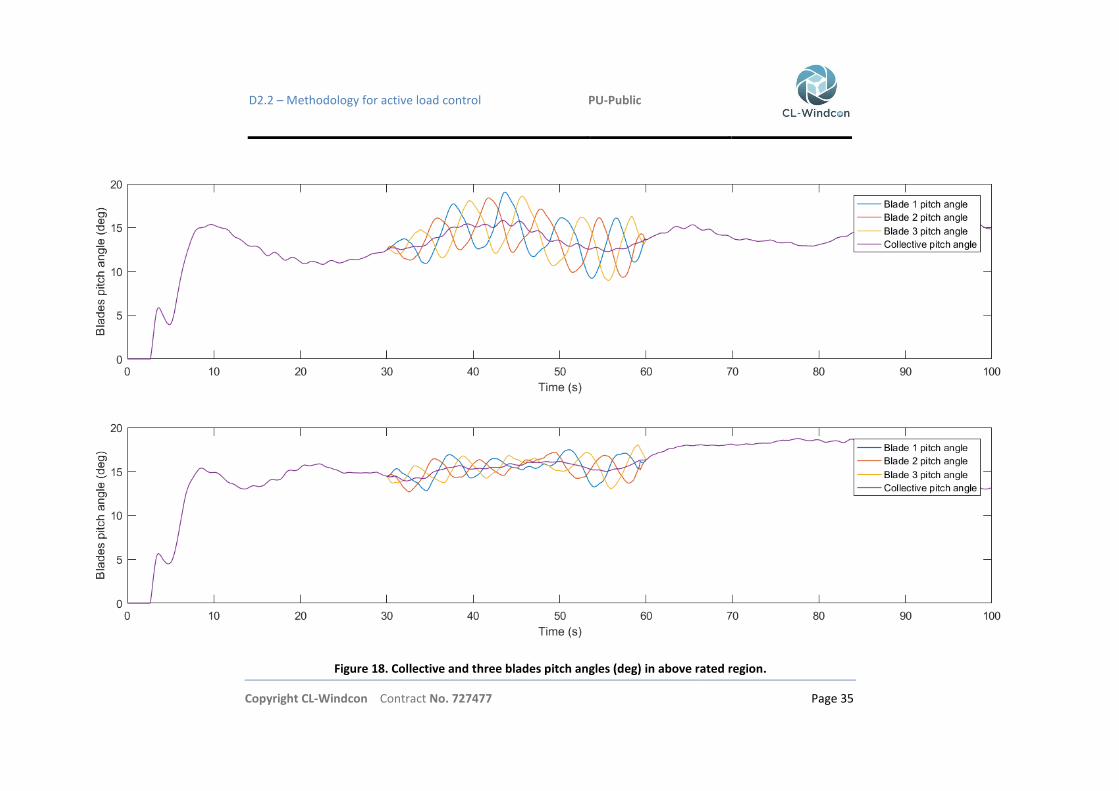
The event is shown in Figure 18, where typical pitch angle variations close to rated wind speed are
depicted [12]. There, it can be seen how the pitch angles of the three blades are superimposed to the
collective pitch angle before and after the event. When the IPC is triggered the angle of each blade
differs, oscillating over the collective pitch angle. This is due to pitch increments from the IPC that are
added to the collective pitch control. The pitches change cyclically to get adapted to the rotor
position, so that highest pitch values are when the blades position is near axis z. Position on which
blades suffer greater loads so an increment of the blade pitch is necessary to reduce lift forces on it.
Unlike lowest pitch values, where loads decrease, so the pitch angle is reduced to compensate the
load variation.

D2.2 – Methodology for active load control PU-Public
Copyright CL-Windcon Contract No. 727477 Page 33
The effect of the individual pitch control can be appreciated in Figure 19 Staring at the figure it can
be noticed a significant difference during the stretch of time IPC is activated, where fewer variations
in blades loads are given. To study the effects of the IPC, a comparison of the fatigue loads would be
necessary. This would be further investigated in future deliverables.

D2.2 – Methodology for active load control PU-Public
Copyright CL-Windcon Contract No. 727477 Page 34
Figure 17. Two seeds of turbulent wind time histories (above rated region).
D2.2 – Methodology for active load control PU-Public
Copyright CL-Windcon Contract No. 727477 Page 35
Figure 18. Collective and three blades pitch angles (deg) in above rated region.

D2.2 – Methodology for active load control PU-Public
Copyright CL-Windcon Contract No. 727477 Page 36
Figure 19. Three blades root moments (kN·m) in above rated region.

D2.2 – Methodology for active load control PU-Public
Copyright CL-Windcon Contract No. 727477 Page 37
Figure 20 and Figure 21 offers an additional point of interest to be observed. Both figures show the
moments and pitches around axes y and z that are inputted and outputted from the IPC controller.
Figure 20 exposes the blade root moments in a fixed frame of reference, My and Mz. Here, clear
effects of the individual pitch control can be seen. In the 30th second of the simulation, when the IPC
is triggered, both moments approach to zero and are maintained around it for the 30 seconds the IPC
is activated, before returning to higher values with no IPC.
Figure 20. My and Mz (kN·m).
In Figure 21 appear the pitch angles y and z in the non-rotating frame of reference outputted by the
IPC controller. As in the previous figure, the impact of the IPC can be easily examined. In this case,
the pitches are non-zero only when the IPC is activated. In the stretch of time IPC is activated, the
controller outputs the necessary changes in pitch angle around axis y and z to achieve the load
reduction shown in Figure 20.

D2.2 – Methodology for active load control PU-Public
Copyright CL-Windcon Contract No. 727477 Page 38
Figure 21. Pitch y and pitch z (deg).
The individual pitch control activates only with above rated wind speeds, where rotor speed is
controlled with the pitch. Due to that, it is interesting to study rated wind speed cases where the
transition between control regions coincides with the IPC. This can be seen in Figure 23, where many
of the seeds meet this requirement. For below rated speeds, pitch angle keeps its optimal value of 0
to absorb the maximum energy from the wind. When the wind speed increases and the control
region changes, the value of the collective pitch angle is increased to reduce loads in the rotor. In
three of the cases shown below this event coincides with the IPC being active. The effect of these
events is highlighted in Figure 24, where three blade loads are shown. When the region transition
occurs, the reduction in blade loads due to the IPC can be clearly seen. This change is not only
noticed in loads variability but also in loads value, which falls rapidly after the pitch control is applied.

D2.2 – Methodology for active load control PU-Public
Copyright CL-Windcon Contract No. 727477 Page 39
Figure 22. Two seeds of turbulent wind time histories (region transition).

D2.2 – Methodology for active load control PU-Public
Copyright CL-Windcon Contract No. 727477 Page 40
Figure 23. Collective and three blades pitch angles (deg) in region transition.

D2.2 – Methodology for active load control PU-Public
Copyright CL-Windcon Contract No. 727477 Page 41
Figure 24. Three blades root moments (kN·m) in region transition.

D2.2 – Methodology for active load control PU-Public
Copyright CL-Windcon Contract No. 727477 Page 42
The controller aims to achieve more reliable conclusions about the functionality of the
implementation, so more situations have been simulated apart from the design load case 1.2. Most
remarkable results have been obtained from simulations of above rated uniform wind combined with
an extreme wind shear. The purpose of this is to analyze the influence of wind shear and the
behavior of the turbine and the individual pitch control in that kind of situation. Some relevant
parameters from a simulation in above rated region are shown in Figure 25 and Figure 26. Extreme
wind shear supposes substantial loading irregularities in blades that depend on the rotor position.
Due to that is an ideal condition to test the individual pitch control. This can be seen in Figure 25
where three blades pitch angles bear huge variations provoked by the IPC output control actions.
Even so, if attention is paid to the plot next to this, three blades root moments, excellent results are
obtained. Not only the value of the loads has decreased, furthermore the variation of loads has had
an outstanding reduction. Higher speeds and shears result in saturation of pitches y and z that can be
possibly fixed increasing the value of the maximum individual pitch set by the trigger, if the
saturation does not occur due to hardware limitations.
Moments and pitches in the fixed frame of reference also appear in Figure 26. As it can be seen, most
changes occur around axe y. This is because only vertical shear has been applied in this case. The two
plots below shows that pitch y increases almost 6 degrees and that My suffers a quick fall
approaching to zero when IPC is activated. Pitch z and Mz just have slight changes, because, as said
before, the wind shear used in the plots is only vertical. For a horizontal wind shear the same results
are obtained, but the opposite happens to the parameters in the non-rotating frame of reference,
pitch y and My are near zero and pitch z and Mz have negative values.

D2.2 – Methodology for active load control PU-Public
Copyright CL-Windcon Contract No. 727477 Page 43
Figure 25. Blades pitch angle and root moments for uniform wind with extreme wind shear (above rated region).

D2.2 – Methodology for active load control PU-Public
Copyright CL-Windcon Contract No. 727477 Page 44
Figure 26. Pitch and moments in the non-rotating frame of reference for uniform wind with extreme wind shear (above rated region).

D2.2 – Methodology for active load control PU-Public
Copyright CL-Windcon Contract No. 727477 Page 45
5 CLOSED LOOP WAKE STEERING
With the growing size of wind turbines and a denser spacing of them in wind farm, the need of new
technologies to mitigate flow interactions has arisen. In the wake of a wind turbine, the wind speed
is reduced and moreover, due to the energy extraction and mixing, the turbulence intensity is
increased. Thus, if a second turbine is impinged by a wake the structural loads are increased and the
power production of that second turbine is decreased compared to the nominal operation in free
stream. Moreover, if the wake impingement is only partially on the rotor due to a partial wake
overlap, the structural loads are even higher since the wind turbine experiences heavily
inhomogeneous inflow conditions.
The concept of open-loop wake steering have been introduced as a methodology to deflect the wake
by either yawing the wind turbine or by cyclic blade pitching such that wake overlaps are avoided,
see [17]. In various investigations the concept has been investigated and the main advantages have
been shown, see [18][19][20][21].
Wake steering, in an open-loop approach, contains the following drawbacks:
Optimized yaw angles are applied in an open-loop approach. Since the yaw angles are computed with
assumptions, e.g. on atmospheric conditions, wind speed, or using a reduced-order model, the
approach does not guarantee that the wake is going to the desired direction. Thus, the
match/mismatch of the assumptions highly influences the control performance.
In an open-loop methodology there is a high sensitivity against disturbances. This means that any
disturbance, e.g. cross wind or shear, will influence the wake position and therefore the achieved
performance.
The concept of lidar-based closed-loop wake redirection, which was first introduced in [22] and [23],
can help to overcome the drawbacks and is presented in the following.
5.1 Objectives
The main objective of lidar-based closed-loop wake steering is to steer the wake to a desired position
by the usage of information provided by a lidar system and a controller that commands the yaw
angle and uses the desired and the estimated position information.
In the following first, the general structure of the concept is presented, as well as the different
subparts, the controller and the estimation task. Then, the implementation and considerations are
presented and finally, conclusions are given.

D2.2 – Methodology for active load control PU-Public
Copyright CL-Windcon Contract No. 727477 Page 46
5.2 General concept of closed-loop wake steering
The lidar-based closed-loop wake redirection concept consists of two main tasks: 1) the estimation
task and 2) the control task. Figure 27 gives the closed-loop scheme of the concept. The control-loop
is closed locally on the turbine level which has advantages in terms of scalability, implementation and
communication. Nevertheless, the estimation task could also be realized on farm level.
Figure 27.The concept of closed-loop wake steering.
The concept shown in Figure 27 mainly consists of two parts: the estimation task and the control
task. The estimation task uses the lidar measurements and provides an estimation of the wake
position to the control task. The control gets the wake position from the estimation task together
with a demanded position and commands the yaw angle to the wind turbine.
In the following, the two tasks are described in detail.
5.2.1 Estimation task
The estimation task deals with providing an estimation of the wake position from lidar measurement
data. In our case we assume a downwind facing scanning lidar system on the wind turbine nacelle.
The lidar system scans a defined measurement trajectory and provides the measurement data to the
control system. Figure 28 visualizes the scan configuration of the lidar system. In this setup, a grid of
7x7 grid points is scanned with a scanning frequency of 1 Hz. Five distances are measured
instantaneously and send to the estimation system. Later, in section 5.3 methodologies are
presented to estimate the wake position from the lidar measurement data.

D2.2 – Methodology for active load control PU-Public
Copyright CL-Windcon Contract No. 727477 Page 47
Figure 28. Measurement trajectory of the scanning lidar system facing downwind.
5.2.2 Control task
The control task deals with everything related to the wake redirection controller. Generally speaking,
it provides the yaw command to the wind turbine by comparing the actual wake position to the
demanded wake position and using this information in the controller (Figure 27 for the general
structure and the inputs and output). There are different approaches how the controller can be
realized. The main challenges are in the robustness of the controller because of having a lot of
unmodeled dynamics in the flow, and the controller design. In section 5.4 a 𝐻∞ controller will be
designed and analyzed.
5.3 Lidar-based wake tracking
As already pointed out, the lidar-based wake tracking, estimates the wake position from the lidar
measurement data. In the following, first the lidar measurement principle is reviewed, then different
methodologies are classified and described, and finally a conclusion is given.

D2.2 – Methodology for active load control PU-Public
Copyright CL-Windcon Contract No. 727477 Page 48
5.3.1 Lidar system
A lidar system is a laser-based measurement device. It uses the Doppler principle to obtain wind
speed information from the backscattered laser light. A lidar system generally has two limitations in
its measurement principle: 1) the lidar measures only a projection of the flow components onto the
laser beam vector, 2) the lidar's volume averaging.
The lidar system only receives parts of the flow components because it uses the backscattered light
to obtain a wind speed measure. Thus, only the projection of the wind flow on the laser is measured,
the line-of-sight wind speed, 𝑣𝑙𝑜𝑠 . Real lidar systems can’t measure at a dedicated point in space as
the idealized measurement equation would impose; however, they measure in a certain volume
around the measurement position along the laser beam. This yields the volume measurement
equation of a lidar to
𝑣𝑙𝑜𝑠 ,𝑖 = 1
𝑓𝑖 𝑥𝑎 ,𝑖𝑢𝑎 + 𝑦𝑎 ,𝑖𝑣𝑎 + 𝑧𝑎 ,𝑖𝑤𝑎 𝑊 𝑎 𝑑𝑎∞
−∞
, (12)
at the measurement point 𝑥,𝑦, 𝑧 𝑖 with the focus distance 𝑓𝑖 = 𝑥𝑖2 + 𝑦𝑖
2 + 𝑧𝑖2, the rage weighting
function 𝑊(𝑎), that depends on the lidar system, see [24], and the flow vector 𝑢, 𝑣,𝑤 𝑖 .
5.3.2 Classification of lidar-based wake tracking methods
The objective of lidar-based wake tracking is to obtain wake position estimation from lidar
measurement data. There are different methodologies which approach the task with different
approaches. Generally, they can be grouped into two categories: template fitting methods and wake
model based method.
The general idea of template fitting methods, are to fit shape or pattern properties, like e.g. a
Gaussian shape or a circular wake shape, to the measurement data. The advantages are the
simplicity of the methods. A disadvantage arises from the discrepancy between assumption and
reality. This means the methodology can mislead gravely if the assumptions are not valid or only valid
in specific cases. Furthermore, the actual wake can’t be recovered from the information.
The model-based wake tracking goes a more systematic way. It uses a simplified wake model and a
lidar model, to provide a general model for the lidar measurements. This general model is then used
in a least-square optimization to fit best to the measurement data. This approach is called wind field
reconstruction and has already been tested in different applications, see [25][26].
In the following, two examples of lidar-based wake tracking are presented, one pattern fitting
method and one model-based approach.
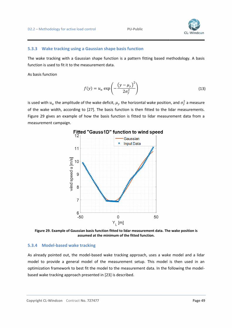
D2.2 – Methodology for active load control PU-Public
Copyright CL-Windcon Contract No. 727477 Page 49
5.3.3 Wake tracking using a Gaussian shape basis function
The wake tracking with a Gaussian shape function is a pattern fitting based methodology. A basis
function is used to fit it to the measurement data.
As basis function
𝑓 𝑦 = 𝑢𝑎 exp − 𝑦 − 𝜇𝑦
2
2𝜍𝑦2 (13)
is used with 𝑢𝑎 the amplitude of the wake deficit, 𝜇𝑦 the horizontal wake position, and 𝜍𝑦2 a measure
of the wake width, according to [27]. The basis function is then fitted to the lidar measurements.
Figure 29 gives an example of how the basis function is fitted to lidar measurement data from a
measurement campaign.
Figure 29. Example of Gaussian basis function fitted to lidar measurement data. The wake position is assumed at the minimum of the fitted function.
5.3.4 Model-based wake tracking
As already pointed out, the model-based wake tracking approach, uses a wake model and a lidar
model to provide a general model of the measurement setup. This model is then used in an
optimization framework to best fit the model to the measurement data. In the following the model-
based wake tracking approach presented in [23] is described.

D2.2 – Methodology for active load control PU-Public
Copyright CL-Windcon Contract No. 727477 Page 50
As described before the general idea is to fit a reduced-order wake model augmented with a lidar
measurement model to the lidar measurement data. Figure 30 shows the general setup of the
approach. An optimizer is used to best fit the “simulated” line-of-sight lidar measurements 𝑣𝑙𝑜𝑠 ,𝑠 to
the lidar measurement data 𝑣𝑙𝑜𝑠 ,𝑚 to obtain the best estimation of model parameters (here named
as best fit wind field characteristics).
Figure 30. The general setup of model-based wind field reconstruction for model-based wake tracking
In the following, first the lidar model is described, and then the wind field model including the wake
model is briefly presented.
For the lidar model description the volume averaging is neglected. Thus, the lidar measurement
equation is approximated with a point measurement equation
𝑣𝑙𝑜𝑠 =1
𝑓𝑖 𝑥𝑖𝑢𝑖 + 𝑦𝑖𝑣𝑖 + 𝑧𝑖𝑤𝑖 (14)
at the measurement point 𝑥,𝑦, 𝑧 𝑖 with the flow vector 𝑢, 𝑣,𝑤 𝑖 and the focus distance 𝑓𝑖 .
The wind field model consists of an ambient homogeneous wind field and a linear vertical shear.
Furthermore, a reduced-order wind field model is used that superpose the wind field. The wind field
model results to
𝑢𝑣𝑤
𝑖
= 𝑣0 + 𝑧𝑖𝛿𝑉 + Ψ𝑢 ,𝑖
Ψ𝑣,𝑖
0
(15)
with 𝑣0 the wind speed, 𝛿𝑉 the vertical shear, and Ψ𝑢 ,𝑖 and Ψ𝑣,𝑖 the 𝑢- and 𝑣- component of the
wake model (depending on the orientation and the model choice) at point 𝑥,𝑦, 𝑧 𝑖 .
For the reduced-order wake model, the dissipation-based wake model is used. We further refer to
deliverable D1.2 for a detailed description of it.

D2.2 – Methodology for active load control PU-Public
Copyright CL-Windcon Contract No. 727477 Page 51
Figure 31 gives an example how the methodology works and compares the result of the fit to the
measured field data. In the first row, the output of the model is shown, in the second row, the
measurement data is seen. The data was measured in five different downstream distances, from 0.6
to 1.4 of the rotor diameter. The estimated wake position is marked with the black dot.
Figure 31. An example of the fit of the general model to the lidar measurement data measured in a field testing campaign.
5.4 Controller design
The main task of the closed-loop wake redirection controller is to use the estimated and the desired
wake position and command a yaw angle, such that the error between them becomes zero. Thus, in
a closed-loop control the wake position is stabilized at its desired position. In the following, first the
controller design model is presented and next a 𝐻∞ controller is designed. Then, the obtained
controller is analyzed in time and frequency domain. The simulations are performed with WFSim,
[28], a two dimensional medium-fidelity Navier-Stokes flow model for wind farm applications. For a
detailed description of the model we refer to D1.2. (Deliverable on control-oriented wake/wind farm
models)
5.4.1 Controller design model
A controller design model is needed to design 𝐻∞ controller. Therefore, a linear model is needed that
gives the input output dynamics of the wake redirection. For the model, the input is the yaw
misalignment angle of the wind turbine that is defined relative to the wind direction. The output is
the estimated wake position of the lidar system at a certain measurement distance. Here, a
measurement distance of 2.5 times the rotor diameter (D) is assumed.

D2.2 – Methodology for active load control PU-Public
Copyright CL-Windcon Contract No. 727477 Page 52
There are different methodologies and approaches for obtaining a controller design model. Examples
for closed-loop wake redirection control are the reduced order modeling of dynamics and
combination with a nonlinear gain function in [22], or model parameterization techniques as done in
[29]. Both approaches give a linear model representation of the form
𝐺𝑖 𝑠 = 𝐾𝑖𝐷𝑖(𝑠) (16)
With 𝐾𝑖 the gain that gives the static wake deflection at a defined yaw angle and 𝐷𝑖(𝑠) the linear
dynamics. The 𝑖 index labels the linearization point 𝛾𝑖 at wind speed 𝑢𝑖 . Here, the model
parametrization is briefly reviewed, because it has also applicability to experimental testing scenarios
and can more easily unknown dynamics.
The model parameterization approach uses experimental data, e.g. step simulations, to obtain a
controller design model. Here, step simulations are performed with the simulation model, WFSim.
Figure 32. The estimated wake position of different step simulations.

D2.2 – Methodology for active load control PU-Public
Copyright CL-Windcon Contract No. 727477 Page 53
Figure 32 gives the results of different step simulations. A step on the yaw misalignment is applied
and the wake position is estimated at 2.5 times the rotor diameter downstream of the wind turbine.
The step simulations show different static behavior (difference in gain) and differences in the
dynamic response (dynamics). A model identifications approach is then used to obtain linear dynamic
models from the step responses. Here, grey box identification is used, where the number of poles
and zeros are predefined and the best model representation is found by the algorithm. Figure 33
shows the bode analysis of the obtained models. For the model identification a number of 𝑛𝑝 = 5
poles and 𝑛𝑧 = 2 zeros are defined. The model order is chosen to achieve a good model accuracy of
with the experimental data while having a low minimum order.
Figure 33. The different models obtained from the model parametrization.The color order is according to Figure 32.
5.4.2 Controller design synthesis
The 𝐻∞ controller design synthesis is applied to the wake redirection control problem in the
following. First, the general design procedure is presented and then the design criteria for the
controller are discussed.

D2.2 – Methodology for active load control PU-Public
Copyright CL-Windcon Contract No. 727477 Page 54
The advantage of 𝐻∞ controller design synthesis is to directly shape the frequency behavior of
performance outputs of the controller during the design procedure. This means, a performance
output like e.g. the output disturbance sensitivity can be directly shaped (within the feasibility of the
problem). The used performance outputs are the output sensitivity S and the controller sensitivity U
that are
𝑆 =1
1 + 𝐺𝐾 (17)
𝑈 = 𝐾
1 + 𝐺𝐾 (18)
𝑇 = 𝐺𝐾
1 + 𝐺𝐾 (19)
where G is the plant model and K the controller. The tracking behavior T is indirectly considered by
𝑆 + 𝑇 = 1 (20)
The shaping is done by applying performance weights to the performance measures. Altogether, this
yields the following minimization problem for the 𝐻∞ controller design
min𝐾
𝑊𝑆𝑆𝑊𝑇𝑇𝑊𝑈𝑈
∞
(21)
With the weights 𝑊𝑆, 𝑊𝑇 and 𝑊𝑈 . The 𝐻∞ controller K then minimizes the minimization problem.
In the following the criteria of the weights are discussed. Two main points need to be considered
when defining the weights, the zeros in the plant model (which can be explained by the delay time
between actuation and measurability of the action at the lidar measurement location), and the
damping at higher frequencies. Therefore, the following weights are chosen in the 𝐻∞ controller
design process: For the output disturbance sensitivity, the weight
𝑊𝑆 =
𝑠𝑀 + 𝑤𝐵
𝑠 + 𝑤𝐵𝐴 (22)
With A the desired disturbance attenuation inside bandwidth, 𝑤𝐵 the desired closed-loop
bandwidth, and M the desired bound on 𝑆 ∞ and 𝑇 ∞ is chosen. The weight on the controller
sensitivity is set to
𝑊𝑈 = 𝐶4
2
𝑠2 + 2 𝑤1𝑠 + 𝑤12
𝑠2 + 𝐶 2𝑤1𝑠 + 𝐶𝑤1 2
𝑠2 + 2 𝑤2𝑠 + 𝑤22
𝑠2 + 𝐶 2𝑤2𝑠 + 𝐶𝑤2 2
(23)

D2.2 – Methodology for active load control PU-Public
Copyright CL-Windcon Contract No. 727477 Page 55
With 𝑤1 and 𝑤2 the design frequencies for controller sensitivity and C = 1000. In this case, the
following values have been set: 𝑤1 = 0.01 and 𝑤2 = 0.05.
5.4.3 Controller analysis
A 𝐻∞ controller is designed with the performance weights as previously described. In the following
first the controller is analyzed in frequency domain. Further, the closed-loop performances are
evaluated. Then in a last step, nominal closed-loop step responses are considered in two different
setups. In a nominal setup first, and second, in two setups with different disturbances. In Figure 34 a
Bode analysis of a 𝐻∞ controller is presented. The controller design model was obtained at a wind
speed of 𝑢 = 8ms−1 and a yaw misalignment change from 0 to 5 deg. The performance of the
controller is evaluated in Figure 35. In the he figure, the sensitivity against output disturbances and
the controller sensitivity are presented. Further, the design margins used in the controller design
process are plotted in black. The controller achieves its desired performance.
Figure 34. The bode analysis of the designed 𝑯∞ wake redirection controller.
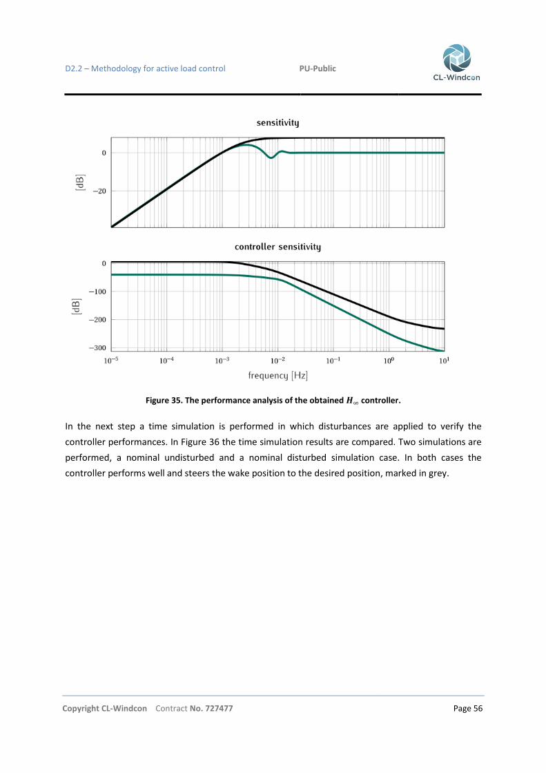
D2.2 – Methodology for active load control PU-Public
Copyright CL-Windcon Contract No. 727477 Page 56
Figure 35. The performance analysis of the obtained 𝑯∞ controller.
In the next step a time simulation is performed in which disturbances are applied to verify the
controller performances. In Figure 36 the time simulation results are compared. Two simulations are
performed, a nominal undisturbed and a nominal disturbed simulation case. In both cases the
controller performs well and steers the wake position to the desired position, marked in grey.

D2.2 – Methodology for active load control PU-Public
Copyright CL-Windcon Contract No. 727477 Page 57
Figure 36. Time simulations with the nominal controller design model.

D2.2 – Methodology for active load control PU-Public
Copyright CL-Windcon Contract No. 727477 Page 58
6 RELIABILITY ENHANCING TECHNOLOGIES
6.1 Objectives
To enhance security and reliability of wind turbines, it is essential to combine monitoring
technologies with the turbine control. These technologies encompass a large variety of sensors and
information transmission methods. Sensors are constantly communicating with the controller,
providing the necessary information for the optimal operation of the turbine. Due to that, the
detection of faults in sensors is vital to avoid damages in the turbine and assure the quality of the
supplied energy. Usually, when a fault is detected in a sensor, the controller will shut down the
turbine for security reasons interrupting the energy production. The following control method has
been implemented so that the operation break can be avoided without losing effectiveness of the
controller, enhancing the reliability of the turbine.
6.2 Design and implementation
The basis of this method is the redundancy of the generator speed monitoring. The use of the
measurements of three sensors is proposed to get the next variables: generator speed, rotor speed
and azimuth [30][31][32].
The speed sensor manager takes the generator speed, rotor speed and azimuth angle
measurements, cross-checks them and outputs a usable generator speed signal when possible.
Figure 37. Speed Sensor Manager block.
These three variables are compared using the relation between them:
𝑅𝑜𝑡𝑜𝑟𝑆𝑝𝑒𝑒𝑑 =𝐺𝑒𝑛𝑒𝑟𝑎𝑡𝑜𝑟𝑆𝑝𝑒𝑒𝑑
𝐺𝑒𝑎𝑟𝑏𝑜𝑥𝑅𝑎𝑡𝑖𝑜 → 𝐺𝑒𝑛𝑒𝑟𝑎𝑡𝑜𝑟𝑆𝑝𝑒𝑒𝑑 = 𝑅𝑜𝑡𝑜𝑟𝑆𝑝𝑒𝑒𝑑 · 𝐺𝑒𝑎𝑟𝑏𝑜𝑥𝑅𝑎𝑡𝑖𝑜 (24)
𝐴𝑧𝑖𝑚𝑢𝑡 = 𝑅𝑜𝑡𝑜𝑟𝑆𝑝𝑒𝑒𝑑 · 𝑑𝑡 → 𝐺𝑒𝑛𝑒𝑟𝑎𝑡𝑜𝑟𝑆𝑝𝑒𝑒𝑑 = 𝑑𝐴𝑧𝑖𝑚𝑢𝑡
𝑑𝑡 · 𝐺𝑒𝑎𝑟𝑏𝑜𝑥𝑅𝑎𝑡𝑖𝑜 (25)
These calculations are pretty accurate approximations; just little mechanical losses of the gearbox
are not taken into account. Due to that, some tolerance is necessary when comparing the
measurements of the sensors, which is done during a determined interval.
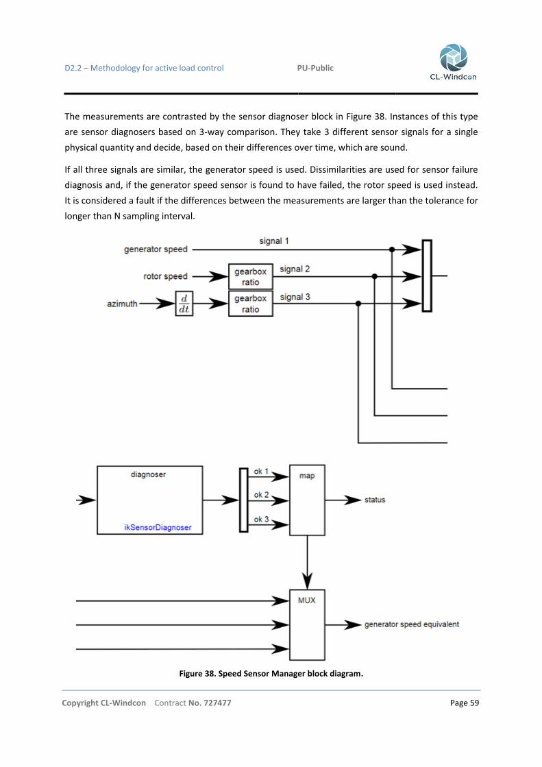
D2.2 – Methodology for active load control PU-Public
Copyright CL-Windcon Contract No. 727477 Page 59
The measurements are contrasted by the sensor diagnoser block in Figure 38. Instances of this type
are sensor diagnosers based on 3-way comparison. They take 3 different sensor signals for a single
physical quantity and decide, based on their differences over time, which are sound.
If all three signals are similar, the generator speed is used. Dissimilarities are used for sensor failure
diagnosis and, if the generator speed sensor is found to have failed, the rotor speed is used instead.
It is considered a fault if the differences between the measurements are larger than the tolerance for
longer than N sampling interval.
Figure 38. Speed Sensor Manager block diagram.

D2.2 – Methodology for active load control PU-Public
Copyright CL-Windcon Contract No. 727477 Page 60
The diagnoses are, 1 for sound sensors and 0 for faulty ones. Depending on the diagnoses the
returned statuses are:
0: all sensors agree
-1: bad generator speed
-2: bad rotor speed
-3: bad azimuth
-4: two or more bad signals
Generator speed equivalent given by the speed sensor manager varies with the returned status. In
Table 2 conditions for different outputs are showed. The value of the generator speed equivalent
matches one of the inputs entered in the MUX block depending on the status. The measured
generator speed is the first input (ok 1), the rotor speed the second (ok 2) and the azimuth the third
(ok 3). This last value is not used as an output.
ok 1 ok 2 ok 3 status MUX
1 1 1 0 1
0 1 1 -1 2
1 0 1 -2 1
1 1 0 -3 1
0 0 1 -4 1
0 1 0 -4 1
1 0 0 -4 1
0 0 0 -4 1
Table 2. Diagnoses map

D2.2 – Methodology for active load control PU-Public
Copyright CL-Windcon Contract No. 727477 Page 61
6.3 Simulation results
To test the speed sensor block a simple generator speed sensor fault introduction facility is provided.
The parameters governing this fault are in ikClwindconInputMod.c. In this file a generator speed
measurement of val is enforced after N sampling intervals. The fault happens in the 100th second
(N=10000, T=0.01 s) and two erroneous generator speed measurements have been tested, 0 rad/s
and 50 rad/s. To avoid false positive error detection, N sampling interval of 2 has been set with a
tolerance of 3 rad/s. Like that, errors provoked by initial values of the simulation and by deviation
between measurements are avoided. An N sampling interval of 2 involves a little delay in the fault
detection. During that delay, an erroneous measurement is used for the generator speed equivalent,
which involves a wrong control of the turbine. Thus, when the fault is detected the controller
responds to the sudden change provoking some transient oscillations. For above rated speeds,
deviation occurred due to the detection delay results in a slight reduction of the pitch angle, which is
rapidly fixed provoking few transient oscillations and negligible loads in blades and shaft. Rated and
below rated loads instead are controlled by electrical torque. This is modified much faster than pitch
angle, so its correction implies pretty high moments in rotor shaft.
For the simulations, six seeds of wind speeds from cut-in to cut-out have been considered with a
normal turbulence mode, as dictated by design load case 1.2. A total run time of 200 seconds has
been simulated, instead of the 600 seconds required by the rule, enough to show the impact of the
fault detection implementation.
Figure 39 shows measurements of the three sensors. Signals 2 and 3, from rotor speed and azimuth
respectively, have really nearby measurements so they look overlapped. Signal 1 samples the
measured generator speed, which is having a breakdown in the 100th second. The event moment is
noticed because the value of signal 1 falls to zero. Thenceforth, signal 2 is outputted as the generator
speed equivalent. So, half of the data coincides with signal 1 and the other half with signal 2,
coupling both data in a single output variable.

D2.2 – Methodology for active load control PU-Public
Copyright CL-Windcon Contract No. 727477 Page 62
Figure 39. Speed sensors measurements for two turbulent seeds in above rated region.

D2.2 – Methodology for active load control PU-Public
Copyright CL-Windcon Contract No. 727477 Page 63
Figure 40. Generator speed equivalent for two turbulent seeds in above rated region.
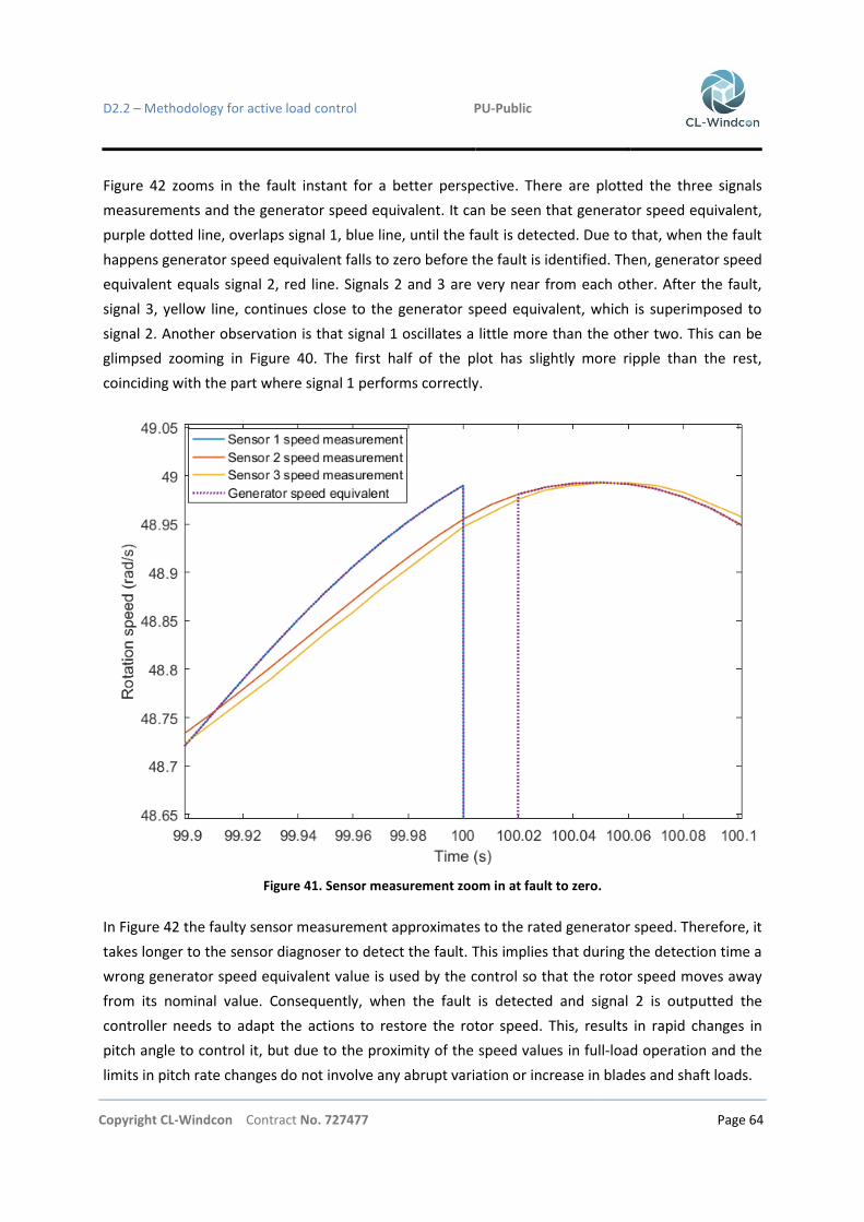
D2.2 – Methodology for active load control PU-Public
Copyright CL-Windcon Contract No. 727477 Page 64
Figure 42 zooms in the fault instant for a better perspective. There are plotted the three signals
measurements and the generator speed equivalent. It can be seen that generator speed equivalent,
purple dotted line, overlaps signal 1, blue line, until the fault is detected. Due to that, when the fault
happens generator speed equivalent falls to zero before the fault is identified. Then, generator speed
equivalent equals signal 2, red line. Signals 2 and 3 are very near from each other. After the fault,
signal 3, yellow line, continues close to the generator speed equivalent, which is superimposed to
signal 2. Another observation is that signal 1 oscillates a little more than the other two. This can be
glimpsed zooming in Figure 40. The first half of the plot has slightly more ripple than the rest,
coinciding with the part where signal 1 performs correctly.
Figure 41. Sensor measurement zoom in at fault to zero.
In Figure 42 the faulty sensor measurement approximates to the rated generator speed. Therefore, it
takes longer to the sensor diagnoser to detect the fault. This implies that during the detection time a
wrong generator speed equivalent value is used by the control so that the rotor speed moves away
from its nominal value. Consequently, when the fault is detected and signal 2 is outputted the
controller needs to adapt the actions to restore the rotor speed. This, results in rapid changes in
pitch angle to control it, but due to the proximity of the speed values in full-load operation and the
limits in pitch rate changes do not involve any abrupt variation or increase in blades and shaft loads.

D2.2 – Methodology for active load control PU-Public
Copyright CL-Windcon Contract No. 727477 Page 65
Figure 42. Sensor measurement zoom in at fault to rated.
Figure 43 and Figure 44, as figures above, show signal measurements and outputted generator speed
equivalent. These cases are for below rated speed, unlike the previous ones that are for above rated
speeds. For these probes turbine is operating in region 2, where a torque control is applied to control
the rotor speed maintaining pitch angle in its optimum value, 0. This control mode is faster so fewer
variations and deviations are given between the three measured signals, but the change between
generator speed equivalent signals is more obvious. This can be clearly seen in Figure 44 due to the
oscillations provoked by the alterations in torque during the fault detection. In this case, while blade
loads are neglectable, rotor shaft suffers considerably more loads because the turbine is operating
with partial load, so rotor speed is controlled with the electrical torque and blade pitch is kept
constant. When the fault is detected the electrical torque is changed much faster than pitch angle,
provoking the high loads in rotor shaft for a few moments. This fact is shown in Figure 45 and Figure
46, where the rapid change in generator torque and the loads provoked in the shaft are plotted.
However, these loads are far from being harmful for the turbine, and due to the rarity of such fault
event, fatigue damages are out of consideration.

D2.2 – Methodology for active load control PU-Public
Copyright CL-Windcon Contract No. 727477 Page 66
Figure 43. Speed sensors measurements for two turbulent seeds in below rated region.

D2.2 – Methodology for active load control PU-Public
Copyright CL-Windcon Contract No. 727477 Page 67
Figure 44. Generator speed equivalent for two turbulent seeds in below rated region.
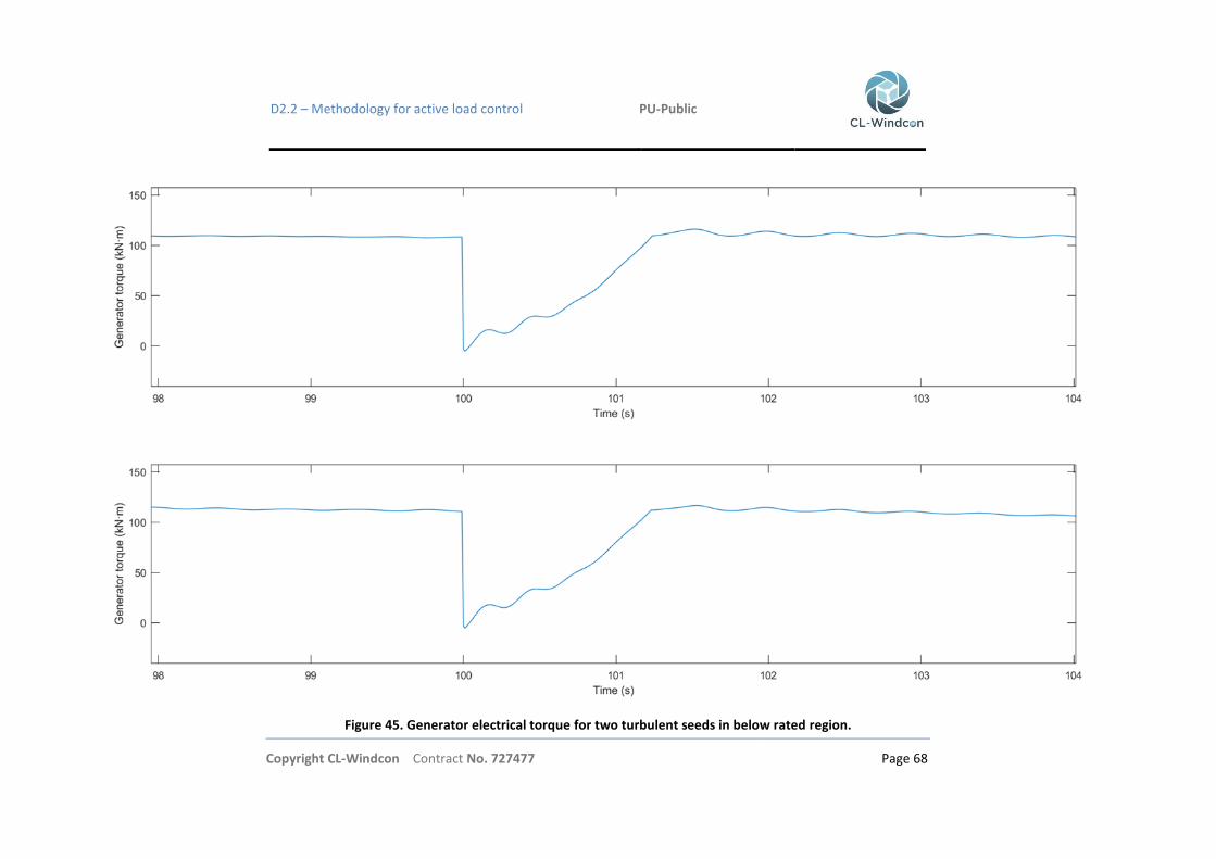
D2.2 – Methodology for active load control PU-Public
Copyright CL-Windcon Contract No. 727477 Page 68
Figure 45. Generator electrical torque for two turbulent seeds in below rated region.

D2.2 – Methodology for active load control PU-Public
Copyright CL-Windcon Contract No. 727477 Page 69
Figure 46. Rotor shaft loads, Mxa, for two turbulent seeds in below rated region.

D2.2 – Methodology for active load control PU-Public
Copyright CL-Windcon Contract No. 727477 Page 70
7 CONCLUSIONS
Chapter 3 has considered the problem of model-updating, in the context of a well-known static
engineering wake model. The model can predict the flow speed within the wake, as well as its
geometry and spatial location depending on environmental and wind turbine operational
parameters. Three possible implementations of the method have been considered. The first tries to
correct model predictions by using power measurements on the downstream turbine. Unfortunately,
the method was shown to fail because of its inability to distinguish between effects caused by wake
speed or position. The second approach uses power to correct only for wake speed. This avoids the
problem being ill-posed, but clearly cannot correct the predictions of the model whenever the wake
position is in error, showing significant errors in maximum power predictions. Finally, a novel method
based on a wake observer is proposed. The wake observer is capable of estimating the local wind
speeds on the left and right sectors of the rotor disk. Clearly, the two velocities carry information on
the actual location of the wake with respect to the affected rotor. This allows one to distinguish
between speed and location, and results in the correct update of both states of the engineering
model. The method can provide valuable information of wake position and reduction, which may be
of high importance for wind farm control applications. It may be interesting for triggering IPC from
chapter 4. IPC demonstrated to reduce considerably loads for above rated wind speeds and different
wind conditions. It makes possible being triggered not only by wake detection, but also other
conditions such as turbine loads.
In chapter 5 the lidar-based closed loop wake steering control concept has been presented. It aims at
redirecting the wake position to a desired position using lidar wind speed measurements, an
estimation of the position from the lidar measurement data and a controller that uses the estimation
to command the yaw misalignment. First the concept is described with its two tasks, the estimation
task and the controller task. The objectives of the two tasks have been described and solutions to
them are presented. Altogether, the concepts enable a closed-loop wake redirection with its
benefits. However, the estimation of the wake position from the measurement data is crucial for the
concept. In the controller task, a 𝐻∞ controller design approach is described and the controller is
derived. It is then analyzed in frequency and time domain with closed-loop simulations. Altogether,
the concept is described and a solution to the weaknesses of the open-loop approach has been
presented. Simulations with different fidelities will be performed in deliverable 3.3 (D3.3).
Finally, chapter 6 has described a fault tolerant control method. Based on the redundancy of the
turbine speed measurement, three different sensor measurements have been cross-checked, so that
a fault in one sensor can be detected by the comparison with the other two and the faulty
measurement can be substituted by a correct one. This method has seemed to be effective in most
cases, just provoking little disturbances in below rated speed cases due to the delay of the detection
and the fastness of the turbine control in that region.

D2.2 – Methodology for active load control PU-Public
Copyright CL-Windcon Contract No. 727477 Page 71
8 REFERENCES
[1] Bottasso, C. L.; Cacciola, S.; Schreiber, J. (2018): Local wind speed estimation, with application
to wake impingement detection. In: Renewable Energy 116, S. 155–168. DOI:
10.1016/j.renene.2017.09.044.
[2] Soltani, Mohsen Nourbakhsh; Knudsen, Torben; Svenstrup, Mikael; Wisniewski, Rafael; Brath,
Per; Ortega, Romeo; Johnson, Kathryn (2013): Estimation of rotor effective wind speed: A
comparison. In: IEEE Transactions on Control Systems Technology 21 (4), S. 1155–1167. DOI:
10.1109/TCST.2013.2260751.
[3] C. L. Bottasso, A. Croce, Cp-lambda Users’s Manual, Tech. rep., Dipartimento di Scienze e
Tecnologie Aerospaziali, Politecnico di Milano (2006e2016).
[4] N.D. Kelley and B.J. Jonkman (2007): Overview of the TurbSim Stochastic Inflow Turbulence
Simulator.
[5] Renkema, Douwe J. (2007): Validation of wind turbine wake models. In: Master of Science
Thesis, Delft University of Technology 19.
[6] C. L. Bottasso, J. Schreiber: Online model updating by a wake observer for wind farm control.
In: ACC 2018 (in review)
[7] Fleming, Paul A.; Gebraad, Pieter M. O.; Lee, Sang; van Wingerden, Jan-Willem; Johnson,
Kathryn; Churchfield, Matt et al. (2014): Evaluating techniques for redirecting turbine wakes
using SOWFA. In: Renewable Energy 70, S. 211-218. DOI: 10.1016/j.renene.2014.02.015.
[8] Keane, Aidan; Aguirre, Pablo E. Olmos; Ferchland, Hannah; Clive, Peter; Gallacher, Daniel
(2016): An analytical model for a full wind turbine wake. In: J. Phys.: Conf. Ser. 753, S. 32039.
DOI: 10.1088/1742-6596/753/3/032039.
[9] Jiménez, Ángel; Crespo, Antonio; Migoya, Emilio (2010): Application of a LES technique to
characterize the wake deflection of a wind turbine in yaw. In: Wind Energ. 13 (6), S. 559–572.
DOI: 10.1002/we.380.
[10] Campagnolo, Filippo; Petrovid, Vlaho; Schreiber, Johannes; Nanos, Emmanouil M.; Croce,
Alessandro; Bottasso, Carlo L. (2016): Wind tunnel testing of a closed-loop wake deflection
controller for wind farm power maximization. In: Journal of Physics: Conference Series 753
(3), S. 32006. DOI: 10.1088/1742-6596/753/3/032006.
[11] Campagnolo, Filippo; Schreiber, Johannes; Garcia, Andrea M.; Bottasso, Carlo L. (2017):
Wind Tunnel Validation of a Wind Observer for Wind Farm Control. In: The proceedings of
the Twenty-seventh International Ocean and Polar Engineering Conference, ISOPE

D2.2 – Methodology for active load control PU-Public
Copyright CL-Windcon Contract No. 727477 Page 72
[12] E. A. Bossanyi, “Individual Blade Pitch Control for Load Reduction”, Wind Energy, vol. 6,
pp.119–128, 2003.
[13] R. Park, “Two reaction theory of synchronous machines”, AIEE Trans. 48, pp.716 – 730, 1929.
[14] T.G. van Engelen, “Design model and load reduction assessment for multi-rotational mode
individual pitch control”, European Wind Energy Conference, Athens, 2006.
[15] S.K. Kanev, T.G. van Engelen, “Exploring the Limits in Individual Pitch Control”, European
Wind Energy Conference, Marseille, France, 16-19, 2009.
[16] Zhongzhou Yang, Yaoyu Li, John E. Seem, “Individual Pitch Control for Wind Turbine Load
Reduction Including Wake Interaction”, American Control Conference, San Francisco, CA,
USA, 2011.
[17] P.A. Fleming, P.M. Gebraad, S.Lee, J.-W. van Wingerden, K. Johnson, M. Churchfield, J.
Michalakes, P. Spalart, and P. Moriarty, “Evaluating techniques for redirecting turbine wakes
using SOWFA,” Renewable Energy, vol. 70, pp. 211–218, 2014.
[18] P. M. O. Gebraad, “Data-driven wind plant control,” Ph.D. dissertation, Delft University of
Technology, 2014.
[19] P. M. O. Gebraad, F. W. Teeuwisse, J. van Wingerden, P. Fleming, S. D. Ruben, J. R. Marden,
and L. Y. Pao, “Wind plant power optimization through yaw control using a parametric model
for wake effects - a CFD simulation study,” Wind Energy, vol. 19, no. 1, pp. 95–114, January
2014.
[20] M. Bastankhah and F. Porté-Agel, “Experimental and theoretical study of wind turbine wakes
in yawed conditions,” Journal of Fluid Mechanics, 2016.
[21] Á. Jiménez, A. Crespo, and E. Migoya, “Application of a LES technique to characterize the
wake deflection of a wind turbine in yaw,” Wind Energy, vol. 13, no. 6, pp. 559–572, 2010.
[22] S. Raach, D. Schlipf, F. Borisade, and P. W. Cheng, “Wake redirecting using feedback control
to improve the power output of wind farms,” in Proceedings of the American Control
Conference (ACC), Boston, USA, July 2016.
[23] S. Raach, D. Schlipf, and P. W. Cheng, “Lidar-based wake tracking for closed-loop wind farm
control,” Wind Energy Science, vol. 2, no. 1, pp. 257–267, 2017.
[24] D. Schlipf, “Lidar-assisted control concepts for wind turbines,” Ph.D. dissertation, University
of Stuttgart, 2016.

D2.2 – Methodology for active load control PU-Public
Copyright CL-Windcon Contract No. 727477 Page 73
[25] S. Kapp and M. Kühn, “A five-parameter wind field estimation method based on spherical
upwind lidar measurements,” in Proceedings of The Science of Making Torque from Wind,
Oldenburg, Germany, 2012.
[26] S. Raach, D. Schlipf, F. Haizmann, and P. W. Cheng, “Three Dimensional Dynamic Model
Based Wind Field Reconstruction from LiDAR Data,” in Journal of Physics: Conference Series:
The Science of Making Torque From Wind, vol. 524, Copenhagen, Denmark, 2014.
[27] L. Vollmer, G. Steinfeld, D. Heinemann, and M. Kühn, “Estimating the wake deflection
downstream of a wind turbine in different atmospheric stabilities: an LES study,” Wind
Energy Science, vol. 1, no. 2, pp. 129–141, 2016.
[28] Boersma, S., Doekemeijer, B., Vali, M., Meyers, J., and van Wingerden, J.-W.: A control-
oriented dynamic wind farm model: WFSim, Wind Energ. Sci. Discuss.,
https://doi.org/10.5194/wes-2017-44, in review, 2017.
[29] S. Raach, J.-W. van Wingerden, S. Boersma , D. Schlipf, P. W. Cheng, „𝐻∞ controller design
for closed-loop wake redirection,” Proceedings of the American Control Conference (ACC),
Seattle, USA, 2017.
[30] Y. Amirat, M.E.H. Benbouzid, E. Al-Ahmar, B. Bensaker, S. Turri, “A brief status on condition
monitoring and fault diagnosis in wind energy conversion systems”, Renewable and
Sustainable Energy Reviews 13, 2629–2636, 2009.
[31] Z. Hameed, Y.S. Hong, Y.M. Cho, S.H. Ahn, C.K. Song, “Condition monitoring and fault
detection of wind turbines and related algorithms: A review”, Renewable and Sustainable
Energy Reviews 13, 1–39, 2009.
[32] P. F. Odgaard, J. Stoustrup, M. Kinnaert, “Fault Tolerant Control of Wind Turbines – a
benchmark model”, 7th IFAC Symposium on Fault Detection, Supervision and Safety of
Technical Processes, Barcelona, Spain, 2009.
[33] T. Burton, N. Jenkins, D. Sharpe, E. Bossanyi, Wind Energy Handbook, ISBN: 978-0-470-
69975-1
[34] Q. Lu, R. Bowyer, B. LI. Jones, “Analysis and design of Coleman transform-based individual
pitch controllers for wind-turbine load reduction”, Wind Energy, 18:1451-1468, 2015.