Demand and Supply Analysis of Voluntary Carbon Credits

Bachelor’s thesisVenla PirhonenAalto University School of BusinessEconomics

1

Aalto UniversitySchool of Business Abstract of bachelor’s thesis

Author: Venla PirhonenTitle of thesis: Demand and Supply Analysis of Voluntary Carbon CreditsDegree: Bachelor’s degree in Economics and Business AdministrationDegree programme: EconomicsAdvisor: Miri StryjanDate: 28 December 2020 Number of pages: 34 Language: EnglishAbstract:Carbon credits transacted in the voluntary carbon markets offer many companies opportunities toreduce their emissions. Because the companies are not obligated to purchase carbon credits by anycompliance scheme, they have other reasons to engage in these markets. However, current literaturedoes not extensively explore the demand factors of voluntary carbon credits. In addition, the creditproducers often find that the production cycle is long and demand hard to anticipate.Therefore, this study analyzes the demand and supply of the markets. Firstly, the demand isanalyzed through a multiple regression analysis of sample companies (N=115). The independentvariables are profit, change in profit, two regions, emissions intensity (total and scope 2), activecompliance regulations, revenue, change in revenue and six different sectors in 2018. Secondly,the supply side is analyzed with credit pricing information.The results of this study indicate a positive and significant relationship between the credit purchasesand changes in profit and revenue as well as being regulated by a compliance scheme. A negativecorrelation is found for purchases and being a retail company. For supply, the analysis concludesa possible imbalance in the project categories, prices and quantities. There is often a shortage offorestry offsets whereas energy projects may have oversupply.Keywords: voluntary carbon trading, carbon credits, demand and supply

2

Table of contents1. Introduction......................................................................................................................................42. Literature review ..............................................................................................................................5

2.1 Voluntary carbon trading........................................................................................................52.2 Supply and demand of offsets.................................................................................................62.3 Factors affecting demand........................................................................................................8

2.3.1 Financial situation ...........................................................................................................92.3.2 Company preferences ................................................................................................................. 102.3.3 Population composition .............................................................................................................. 132.3.4 Future expectations on regulation ............................................................................................ 13

2.4 Factors affecting supply........................................................................................................142.4.1 Production costs ........................................................................................................................... 152.4.2 Technology ................................................................................................................................... 162.4.3 Future expectations ..................................................................................................................... 16

3. Methodology for demand analysis.................................................................................................173.1 Sample selection ...................................................................................................................173.2 Collection of data..................................................................................................................183.3 Analysis of Data ...................................................................................................................193.4 Analysis of variables.............................................................................................................203.5 OLS Assumptions.................................................................................................................21

3.5.1 Linearity......................................................................................................................................... 213.5.2 Normality of Residuals ............................................................................................................... 223.5.3 Exogeneity..................................................................................................................................... 223.5.4 Homoscedasticity......................................................................................................................... 223.5.5 Expected Value of the Error Term ........................................................................................... 223.5.6 Lack of Multicollinearity ........................................................................................................... 23

4. Results of demand analysis ............................................................................................................234.1 Descriptive statistics .............................................................................................................23

4.1.1 Non-binary variables................................................................................................................... 234.1.2 Binary variables ........................................................................................................................... 25

3

4.2 Assessment model through OLS ..........................................................................................264.2.1 Linearity......................................................................................................................................... 264.2.2 Normality of residuals ................................................................................................................ 274.2.3 Exogeneity..................................................................................................................................... 274.2.4 Homoscedasticity......................................................................................................................... 284.2.5 Expected value of error term ..................................................................................................... 284.2.6. Lack of multicollinearity........................................................................................................... 284.2.7 Adjusted regression model ........................................................................................................ 28

4.3 Regression results .................................................................................................................295. The demand and supply model ......................................................................................................31

5.1 Demand model......................................................................................................................315.2 Supply model ........................................................................................................................33

6. Discussion and conclusion .............................................................................................................36References ..........................................................................................................................................38Appendix A: Linearity .......................................................................................................................44Appendix B: Normality of residuals ..................................................................................................46Appendix C: Lack of multicollinearity ..............................................................................................46

4

1. IntroductionVoluntary carbon trading has emerged as one of the most effective methods for organizations, suchas Nestle and Disney, to reduce their carbon footprints (CDP 2020; Abdallah et al. 2012). This thesisprovides an analysis of general voluntary trading patterns as well as a deep dive into the purchases ofsome of the largest and most influential companies. The focus is on the quantitative aspect becausethere is currently a lack of quantitative data and knowledge about the voluntary markets (Kountouriset al. 2014). This is partly due to the market being relatively new, scattered and loosely regulated(Benessaiah 2012). For example, the voluntary market does not have a regional or national controllingbody or common tracking system, causing many transactions never being captured in statistics,especially if no compliance scheme exists in the area the company is based in (ibid.). On top of thisespecially the changes in demand can be hard to predict (Borden 2020).To quantify the purchases of the world’s 200 largest companies, ranked according to their annualrevenues, this paper uses the Carbon Disclosure Project (CDP), an extensive database capturing theclimate information of many major companies. Another key source in this study is credit pricing datafrom Ecosystem Marketplace that performs annual surveys of the field experts and trade participants.The paper has two main angles: demand and supply. These are analyzed first separately, and then theresulting model of demand and supply is examined. More specifically, in the second chapter of thisthesis, existing literature is surveyed for the factors affecting demand and supply of voluntary credits.After this, in the third chapter, the methodology for demand analysis is established. This is followedby the fourth chapter with the quantitative analysis of demand and brief presentation of the results.This analysis consists of a multiple regression of the sample population against different variables,possibly affecting the demand. Thereafter, in the fifth chapter, the implications of these results againstthe demand model are examined. This chapter also includes assessment of the supply model, usingpricing information. Finally, in the sixth chapter, a discussion and conclusion are provided.All in all, the two research questions this paper analyses are 1) the possible correlation between certaincharacteristics of the sample companies and their carbon trading patterns and 2) the model of demandand supply that can fit the voluntary carbon markets.

5

2. Literature review2.1 Voluntary carbon tradingThe emissions trading market emerged initially to tackle one of the major global challenges: to reducethe world’s greenhouse gas (GHG) emissions (Abdallah et al. 2012). The trade can be eithercompulsory or voluntary, depending on whether the participant is obligated by a trading scheme, suchas California Cap and Trade or the EU ETS. This paper focuses on voluntary trading, the importanceof which lies in that it gives companies direct control over their carbon footprints. This control isneeded in times when full emissions regulation does not yet reach many sectors and companies(Spiekermann 2013). Instead of being obliged by law, these companies are often drawn to loweringtheir emissions due to financial incentives and outside pressure (Abdallah et al. 2012). In addition,carbon trading is often easier and quicker to implement than other operational changes, such as useof less polluting raw materials and methods (ibid.). This is especially true in heavy-pollution sectors,such as transportation and manufacturing (ibid.).Voluntary carbon trading enables companies wishing to reduce their carbon footprints to invest in acause to both better the environment and elicit a social impact on the community. The carbon credits,equalling one metric tonne of carbon (tCO2), are produced through a carbon project (Hamrick andGallant 2017). These projects can either reduce emissions or improve carbon sequestration. Theycommonly cover areas, such as forestry or land use, renewable energy, household efficiency andswitch to less-polluting fuels (ibid.). Additionally, the project is usually certified by at least onecarbon standard before it is sold to ensure the credibility of the offsets. These standards check theproject for some common requirements, such as additionality (the reductions would not havehappened without the project) and permanency (ibid.). However, the standards also have differencesin how they operate, and consequently have differing average demands and credit prices (Donofrioet al. 2019). For example, Verra standard, certifying the largest amount of carbon credits in 2019,puts high emphasis on social issues of its projects (Donofrio et al. 2020.; Borden 2020). Indeed, thesocial impact of a carbon credit can be significant for its demand and market value: the offsets withadditional social impact stamp became the most sold category in 2018 and 2019 and these creditssometimes acquire a price premium (ibid; Donofrio et al. 2019).The urgent need for emission cuts in is evidenced by the constant rise in global GHG emissions sincethe beginning of the 21st century (EU Science Hub - European Commission 2020). Because of thisconcerning trend, recent estimates calculate that yearly reductions of more than 7 per cent will beneeded between 2020 and 2030 to meet the Paris Agreement 1,5°C goal (ibid.; UN Environment

6

Programme 2019). In line with this, voluntary carbon markets have attained attention as a prospectivesolution and acquired a yearly trade volume of nearly 100 million tonnes of carbon in 2018 (Donofrioet al. 2019).While carbon trading has positive environmental and social impacts, the companies reducing theiremissions often care about the positive image associated with the reduction reports (Ma et al. 2019;Conte and Kotchen 2010). However, to be able to make convincing reduction statements, companiesmust first accurately calculate their baseline emissions. A company’s emissions can be divided intoscope 1, scope 2 and scope 3 emissions. The Greenhouse Gas Protocol, one of the most importantstandard-setting organizations in carbon accounting, defines scope 1 emissions as the direct emissionsfrom company-owned or controlled equipment, scope 2 as indirect emissions from purchased energyand scope 3 as all other indirect emissions (The Greenhouse Gas Protocol n.d.). Furthermore, scope2 emissions are typically reported as location-based or market-based: location-based values relate tothe emissions from the location where the emissions occur whereas market-based values are theemissions from the energy the company is purchasing (The Greenhouse Gas Protocol 2015).

2.2 Supply and demand of offsetsThe supply of carbon credits is made out of the credit-originating organizations and the demand ofthe customers. If these two actors meet and the trade is efficient, both sides will maximize theirbenefits. Theoretically, then the aggregate price of the transactions in a market reflects the equilibriumquantity and the total yearly quantity reflects the equilibrium price (OpenStax Economics 2016). Thisbalance is the intersection of the two curves, plotted against quantity and price. Moreover, if, forinstance, the preferences of the consumers or the expense of production change, these curves can shift(ibid.). This in turn creates a new balance with a new equilibrium price and quantity.Because carbon trading is a rather new concept and its scope still small, with 2018 net value estimatedat 296 million USD, the research on supply and demand is sparse (Donofrio et al., 2019). Spiekermann(2013) estimated the supply to be in its simplistic form a linear, upwards pointing “marginalabatement cost” line. The demand, on the other hand, exhibits a round shaped downwards curve inSpiekermann’s model: the first portion is extremely elastic and second portion extremely inelastic.This shows that when the price is high, a small reduction in the price elicits a bigger increase indemand than when the price is already low. In addition, this implies that supply quantity is morereactive to shifts in demand than demand is of shifts in supply when the price is low. This relationshipis sometimes observed by the industry leaders: in an interview with the credit certifier Verra, Borden

7

(2020) explains that supply is more easily predictable than demand, and that it can be “hard to get anaccurate picture of demand”. Figure 1 presents an example of the supply and demand when the priceis low.

Figure 1: Model of supply and demand with low price, according to Spiekermann’s (2013) model. S standsfor supply and D for demand. The equilibrium point (q,p) is where supply and demand meet.

In 2018, the average price for a metric tonne of CO2 offset stood at 3.01 USD (Donofrio et al. 2019).Moreover, about half of the voluntary credits that year were sold at a price lower than 1 USD pertCO2 (World Bank Group 2019). This price level is considered low by some (Spiekermann 2013;Benessaiah 2012). Moreover, the compliance market has typically a price-level higher than thevoluntary, and for example, the Paris Agreement expects prices around 40-80 USD per tCO2(Donofrio et al. 2019). A low price-level would point to current demand being on the inelastic side,implying that a lowering of price will not increase the demand significantly. However, Tong et al.(2019) found that at a market price of more than 3 USD, the marginal cost of a carbon credit becomeshigh and companies may find internal reductions more profitable. On the other hand, at lower prices,it is easy for companies to make reductions, seen as an inverse relationship, where the reduction rateincreases as the credit price decreases (ibid.). This study, though, is related to reductions undercompliance systems where a set level of emissions needs to be achieved (ibid.). Therefore, althoughthe result appears contradictory to Spiekermann’s theory of inelasticity (2013), it might only hold ifthe companies are obliged to reduce.

8

However, the situation is never stable as outside factors influence both the supply and demand curves.Common examples of factors affecting demand in a market are income or available funds,preferences, change of population composition and changes in expectations. For supply, in generalproduction costs, new technologies, governmental rules and expectations are shifting factors.According to this theory, if the production of carbon credits becomes more expensive, the supplycurve will shift upwards, causing, other factors remaining constant, the equilibrium point to be at ahigher price and lower quantity. On the other hand, if consumers’ preference for carbon creditsincreases, the demand curve will shift to right and equilibrium point to a higher price and higherquantity. (OpenStax Economics 2016)When both the supply and demand shift, the combined effect determines the new equilibrium pointas seen in figure 2. To better understand the relevant factors for voluntary carbon trading, the literatureon both demand and supply side factors are studied.

Figure 2: A shift in both supply and demand leads to a combined effect. Here both changes increase pricelevel but only demand shift increases quantity. S’ and D’ represent new supply and demand curves. Originalmodel is by Spiekermann (2013).

2.3 Factors affecting demandAs the theory presented by OpenStax Economics (2016) suggests, the main causes of shifts in demandare financial situation, preferences, population composition and future expectations. The relevanceand applicability of these factors to voluntary carbon trading is discussed next.

9

2.3.1 Financial situationIf the financial factor is relevant in the voluntary trade setting, financial performance and carbonreductions may be correlated. The relationship may stem from either offsetting activities beingfinancially beneficial or better financial performance allowing for purchase of more reductions.Current literature does not extensively explore the connection between carbon offsetting and financialperformance. Therefore, to increase the pool of available studies, firstly the connection betweencompanies’ financial performance and general carbon emissions change is established. Most studiesobserve the relationship from the angle “do decreases in emissions lead to better financialperformance?”. For example, Okereke and Russel (2010) state that financial opportunities and threatsrelated to climate change are some of the main drivers of company climate action. However, if thiskind of correlation is found, direction of the effect may also go the other way: better financialperformance leads to better carbon performance.One of the studies exploring the correlation, by Lewandowski (2017), analyzes carbon performancechanges against different parameters of financial performance and finds a general curvilinearrelationship where companies with high baseline pollution values experienced negative financialeffects whereas companies with low values received benefits. In other words, companies that startedout with low emissions experienced a simultaneous increase in financial and climate performance.Another study found both clean and polluting industries to have a negative relationship betweenemissions and ROI (Ganda and Milondzo, 2018). However, the study showed inconclusive resultsagainst other measures of financial performance (ibid.). Lastly, a large meta-study of the relationshipfound a positive connection between relative carbon performance improvements and various financialparameters (Busch and Lewandowski 2017). Overall, the results indicate that there is a positiverelationship between financial and carbon performances, especially for companies that have lowerbase emissions and when looking at the relative changes of the parameters. Therefore, a variable offinancial performance will be included in the analysis.If the baseline emissions are relevant to the financial benefits the companies receive when buyingcarbon offsets, then defining and understanding the variable is important. When it comes to factorsrelated to baseline emissions, Goldhammer et al. (2016) found the company’s revenue to be the mostsignificant variable, explaining between 55 - 86 percentages of the variations. This makes sense asbigger companies often produce in larger scale or have more operations. Because the sample is formedby taking the companies with largest revenues, it may be biased towards high polluters. Moreover,one could hypothesize that small companies with small revenues, and thus smaller mostly baseline

10

emissions, would be more financially motivated to reduce their carbon footprints than companieswith larger revenues. However, this might not be true because, even under compliance schemes,larger companies are allocated more emission permits (ibid.). This can imply that a more pertinentchoice for baseline emissions could be a relative figure instead. Relative comparison will be made inthis study using a carbon intensity figure: carbon emissions divided by revenue from that year(Lewandowski 2017). This allows for even a larger company to have a low carbon intensity numberand already includes the revenue factor. Moreover, Goldhammer et al. (2016) did not find aconclusive connection between intensity of location-based scope 2 emissions and baseline carbonfootprint. It remains unknown if scope 1 or combined scope 1 and 2 emissions are correlated toemissions.All in all, the companies that improved or had good financial performance seem to be more motivatedto reduce their carbon footprints, especially concerning the low polluters. Whether this willingnessleads to carbon credit purchases is not widely explored in literature. In this study, the hypothesis isthat is does to some extent. To assess this, financial performance and credit purchases are compared.Financial performance is analyzed through profits and change in profit. Literature, such as (Buschand Lewandowski 2017), found changes in financial performance to be more significant. Therefore,the hypothesis is as follows:H1: There is a positive correlation between the number of carbon credits bought and profit, andbetween carbon credits bought and change in profit.Another question raised by the theory is on a possible correlation between baseline carbon intensitylevels and reductions, since different levels of emissions are sometimes associated with differentincentives to make reductions. To elucidate the baseline effects, the analysis includes relativeemissions values analyzed through both total and energy-related scope 2 values. The literaturesuggests that there might be a small, negative correlation to purchased carbon credits as smallerpolluters might gain more from reducing their footprints. The second hypothesis is:H2: There is a negative correlation between baseline emission intensity and purchased carboncredits.2.3.2 Company preferencesApart from financial situation, preferences of the companies are also likely to be relevant in the carbontrading setting. The different stakeholder groups of the companies tend to express increasing intereston climate issues and pressure the companies to improve their carbon performances (Galán-

11

Valdivieso et al. 2019). While these stakeholder preferences become part of the preferences of thecompany, the preferences of some groups are often given more weight than others, as Dohnalova andZimola (2013) discovered in their survey of Czech companies. They rank the stakeholders from themost to least important – owners, customers, managers, suppliers and employees (ibid.). Moreover,Dahlmann (2017) explains that common motivations for a company to engage in general emissionsreductions include increased climate-awareness amongst consumers and potential employees,concerns about company legitimacy, attracting investors and matching competing companies.Because owners and investors closely relate to the financial aspect of previous section and employeesare sometimes considered the least influential group, in this section only the impact of preferences ofcustomers and managers are explored (Dohnalova and Zimola 2013). As with the financial analysis,where there is little data on of carbon credit induced reductions, literature on general emissionreductions is analyzed instead.Consumer environmental preference (CEP) refers to the degree customers prefer low-carbon productsand services; a high CEP setting is often found to entice companies to invest in lowering emissions(Tong et al. 2019; Du et al. 2016). This can be due to increased sales numbers and profits fromoffering customers the kind of products they prefer (Tong et al. 2019). Additionally, high CEPcustomers are often willing to pay a premium for low-carbon products (Ngilangwa 2015). Somecompanies face more environmental pressure from the customers than others: for example, acrossdifferent countries there are substantial variations in the environmental preferences and awareness ofthe consumers (Lee et al. 2015). There are also differences across business sectors, partly due todiffering regulation and baseline pollution (Luo 2017; Okereke and Russell 2010). However, Aghionet al. (2020) found that throughout questionnaires and nations, the general trend was reducing CEPbetween early 1990s and 2010 and growing CEP ever since. This general trend could also indicate arising demand for carbon credits since around 2010. Yet CEP is only one factor the companyconsiders and others, such as the state of the compulsory markets, may complicate the picture: asDonofrio et al. (2019) explain, there have been significant fluctuations in the global yearly transactedvolume with no observable increase since 2010.Because the differing customer expectations are hard to capture for each company, a numeric CEPvariable will not be used in this study. The variables potentially catching some of the CEP effect arethe dummies grouping the companies by sector and region. However, due to the limited size of thesample and the resulting broad grouping of the companies, these variables might fail to providespecific insights. Moreover, the explored literature does not give enough support to form a hypothesis

12

related to sector’s effect. However, one hypothesis is made. For region analysis, Lee et al. (2015) findthat Europe and North America have, on average, significantly higher climate change awareness thatother regions. On average, the difference in proportion of population knowing about climate change,between developing countries and the two highest-scoring continents is over 30 percentage points(ibid.). This difference in public awareness could consequently lead to higher rate of carbonoffsetting. The hypothesis is:H3: There is a positive correlation between carbon credit purchases and the two binary variablesdescribing headquarters in Europe and North America.The case of difficult quantification also applies to manager preferences. In general, managers can bemotivated to advocate for reduced emissions to maintain a good company image (Okereke and Russel2010; Dahlmann 2017). The company image, closely related to the company’s legitimacy, can beundermined by poor carbon performance (Galán-Valdivieso et al. 2019). To counteract lowlegitimacy, the company may either try to portray the operations in a more favorable way or makeactual changes. Indeed, some studies found that companies often report more emission-relatedinformation if their legitimacy is low (Ma et al. 2019; Luo 2017). However, stakeholders cansometimes see through such attempts, and in these cases an active carbon policy is found to besignificant in attaining better legitimacy (Galán-Valdivieso et al. 2019). The chosen course of actionmay partly depend on the experiences and views of the managers: for example, Ma et al. (2019)explain that managers with an MBA degree are more climate change aware and engaged in corporateclimate policies. Also, the gender and age of managers can be influential (ibid.). Companies that havemanagers with these kinds of attributes might be more likely to engage in carbon trading. In thisstudy, the manager aspect will not be considered due to the difficulty of finding comparable data. Inaddition, the legitimacy aspect is hard to measure for each company.However, high polluters may have lower legitimacy, and the emission variable may catch somelegitimacy-related information (Ma et al. 2019). The second hypothesis may therefore cover part ofthe legitimacy aspect. Yet overall, the company preferences, whether from customers or innerstakeholders, are difficult to quantify and compare. Moreover, it is likely to affect the company’sengagement in carbon trading to some extent. This effect, if relevant, is not captured in this analysiswhich may weaken the model as a collection of significant factors.

13

2.3.3 Population compositionBecause different companies buy different quantities of carbon offsets and have different preferences,changes in the composition of the largest companies could also change the demand for offset withinthe group. An angle that is looked into in this study is the impact a company’s sector has on itsanticipated carbon trading activity. If, for example, oil and energy companies are found to buy moreoffsets than other sectors, higher concentration of these companies in the top 200 would result a higherdemand for offsets in the data analyzed. However, in this study only 2018 figures for all the variablesare included and, therefore, changes in population composition will not be observed.2.3.4 Future expectations on regulationCompanies that expect to be regulated by a compliance scheme often increase their voluntaryoffsetting prior to this (Donofrio et al. 2019). This pre-compliance impact can also be seen in the bigscale: for example, in 2008 the global sales value of voluntary offsets more than doubled comparedto previous year due to anticipated compliance scheme in the US (ibid.). In general, these pre-compliance companies are also found to be more aware of climate impact and willing to pay a higheramount for less polluting technology (Zhao et al. 2018). Anticipated regulation also increases thetendency of the companies to incorporate a climate policy (Galán-Valdivieso et al. 2019). The goalof these pre-compliance companies is to be adequately prepared when the regulation is implementedand to alleviate the impact of the regulation (ibid.). Additionally, all these actions might later onimpact the company’s internal carbon-related awareness and preferences.Therefore, a tightening regulation may lead to a temporary peak in voluntary trade quantities andmarket value as well as increased general climate change awareness in companies. The ongoing ParisAgreement is one example of a potential cause for increased ambitions for carbon emission reductionsby companies (The Gold Standard 2020a; Borden 2020). On the other hand, after the regulation isestablished, the companies may reduce their investments in the voluntary side to, for example, financethe compliance requirements. In the analysis, a variable for regulation is studied to detect anydifferences. The direction of the effect is not clear from the literature, and therefore, the two-tailedhypothesis is:H4: There is a correlation between whether company is regulated by a compliance scheme and thecompany’s carbon trading activity.All in all, the following hypotheses are formed:

14

Figure 3: Hypotheses derived from literature.2.4 Factors affecting supplyIn this section, three supply shifters – changes in production costs, availability of technology as wellas legislation and other future expectations – are explored in the voluntary trading context. Thesefactors are commonly stated as having an influence on the general supply curve (OpenStaxEconomics 2016). However, a notable point for carbon trading that can reduce the impact ofespecially short-term shifters is that initiating a carbon project usually takes about 2-5 years and thecredits are actively being sold about for another 3-4 years after their issuance (Donofrio et al. 2020;Hamrick and Gallant 2017; Seeberg-Elverfeldt 2010). This can create a substantial lag for someoffsets from the time the implementation planning started to the time the offsets are sold. The delaymight lead to a reduced responsiveness of supply quantity the shifting factors and the demand.Moreover, future expectations may have higher impact than the other shifters.A second important consideration for carbon trading supply is that it may vary significantly amongthe seven commonly named project categories – forestry and land use, renewable energy, fuel switch,household devices, waste, transportation and manufacturing (Donofrio et al. 2020). While onecategory might experience difficulties in production process or uncertainty, typically another categoryis more stable. A good example of this are forest related offsets: although they are consideredcontroversial by many and sometimes difficult to initiate, their demand is usually steady (Conte andKotchen 2010; Borden 2020). Therefore, their supply is also steadier than that of renewable energyor fuel switch (Hamrick and Gallant 2017).

Carbonoffsetting activity

Financial situationH1: Profits andchange in profits

H2: Baselineemissions

Preferences H3: Region

Regulation H4: Complianceschemes

15

2.4.1 Production costsProducing a carbon project is a multistage process. The different types of producer costs associatedwith the projects can be divided into two groups: operational costs and transaction costs (Cacho et al.2013; Cao et al. 2020). If some part of the production process, for example in the transaction course,becomes more expensive, the supply curve is likely to shift to the left, decreasing the sold quantities.The first stage of carbon credit project development is the planning stage (Hamrick and Gallant 2017).At this stage, the project developer usually conducts a feasibility study, prepares project designdocumentation and collects data (Seeberg-Elverfeldt 2010). There might be significant operationalcosts involved. For example, the producer has to often consider the opportunity cost related to theplanned activity, commonly due to the space and resources consumed in the project. Forestry projects,such as reforestation or afforestation projects often come in the place of agricultural or commercialforest land. Therefore, the landowner may require a compensation for this loss of income. In addition,the transaction costs of project design consist of making all the calculations and measurementsrequired, often regarded as the costliest step of the production cycle (Cacho et al. 2013; Arnoldus andBymolt 2011).The second phase is the project validation and verification (Hamrick and Gallant 2017). The typicalsteps are validation of the project plan, consultation with a standard-setting organization, initialverification, and registration of the project (Seeberg-Elverfeldt 2010). At this stage the fulfillment ofproject requirements is checked by external auditors and the certifier. All in all, the main costsassociated with this stage fall in the transaction costs category (ibid.). The third phase is theimplementation of the project (ibid.). This requires project management, monitoring and continuousverification (Cacho et al. 2013). Both operational and transaction costs are acquired. Operating costscan include rent paid to landowner and upkeep of the activities. The transaction costs relate to theinspections and auditing processes necessary to keep the project standard certified. Additionally,finding a buyer can be costly and challenging: even though the market has in general high demand inrelation to supply, many projects fail to find a suitable buyer (Borden 2020; Hamrick and Gallant2017).The total production costs vary based on the size of the project, the chosen standard organization anddifferent characteristics of the project (Donofrio et al. 2019; Conte and Kotchen 2010). However, theproduction costs are relatively stable as the same type of production process with similar stages hasbeen in use for over ten years (comparing information by Hamrick and Gallant (2017) and Seeberg-Elverfeldt (2010)). Many of the largest certifying organizations have similar types of project

16

requirements that typically change only slowly (Michaelowa et al. 2019). Commonly the transactioncosts amount to about 200,000 USD (Seeberg-Elverfeldt 2010). For example, for forestry projects,adding in the operational costs will bring up this number by about 40% (Cao et al. 2020). However,unexpected events, such as conflicts and natural disasters could sway the costs. In addition, newtechnology could bring the costs down, while stricter and more unified certification rules couldincrease the costs. These factors are discussed next.2.4.2 TechnologyTechnology in the carbon trading setting can relate to tools that facilitate the practical implementationand management of the project. Another use for technology is to navigate the extensive verificationand validation requirements. In both cases, availability of more advanced technical solutions canmake it easier for project developers to create and maintain projects, and thus increase the supply ofprojects. This can be important because the current long time it takes for developers to implement aproject points to high barriers for suppliers.Another important benefit brought by technological advancements is increased accuracy, potentiallycreating larger margins for suppliers and, in the larger scale, more credible offsets. A case in point:Iizuka and Tateishi (2015) compare the case of remote sensing technology, such as satellite images,to field manual measurements for forest carbon projects. Compared to man-made calculations andestimates, the solution takes more factors into consideration and is found to be significantly moreaccurate. Overall, due to current impreciseness and risks for unpredictable events in forestry projects,most certifying standards take 10-20% of the credits as a buffer that will only be released at the endof the project period (Phelps and Hoffer 2020). Yet, forestry is one of the most common projectcategories, with the largest sales value of all projects in 2019 (Donofrio et al. 2020). The other largecategories, such as renewable energy, are also likely to benefit similarly from technologicalinnovation.2.4.3 Future expectationsDue to the lengthy time span of projects, long-sighted future expectations may be more significantthan shorter changes. As mentioned about the demand side, potential new climate legislations areoften observed to induce a pre-compliance increase in demand. However, many project developerssee past these bumps and consider potential compliance schemes as threats (Hamrick and Gallant2017). The new Paris Agreement might be perceived as a threat as well because more governmentsare committing to climate goals and becoming more aware of carbon emissions (ibid; Hermwille andKreibich, 2016). This could lead to national carbon inventories that make international voluntary

17

trade difficult. In addition, some suppliers are already looking for possibilities for their voluntarycredits to be recognized by compliance schemes (Hamrick and Gallant 2017).Other future expectations, such as increasing demand for some project category or for social co-benefits in carbon offsets, also change the supply patterns (Donofrio et al. 2019). For example,demand for double certified offsets with a social benefits stamp has been emerging since 2012,increasing rapidly to a top category in the past years (ibid.). This changes the supply, although oftenwith the previously mentioned delay. However, as a whole, the future expectations can be assumedto be more likely to change, and thus cause supply shifts, than the other two factors.

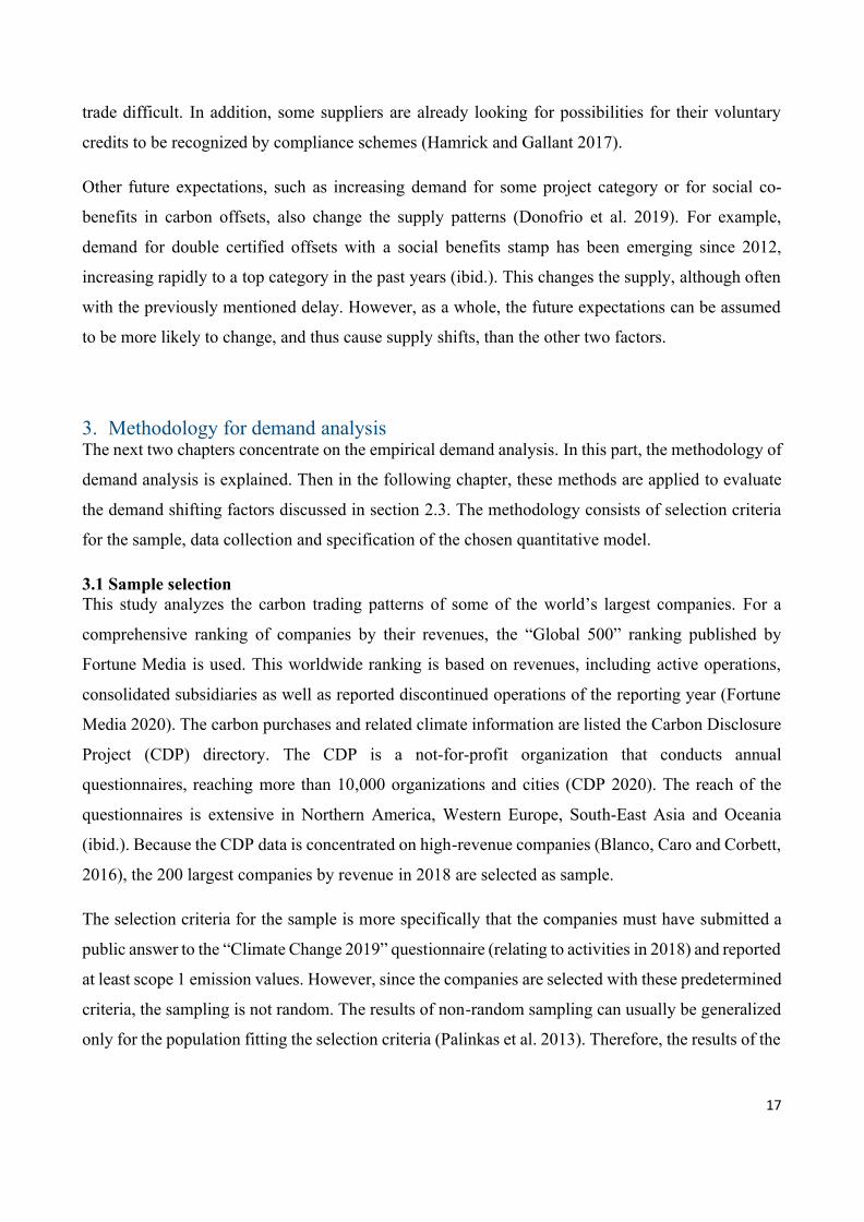
3. Methodology for demand analysisThe next two chapters concentrate on the empirical demand analysis. In this part, the methodology ofdemand analysis is explained. Then in the following chapter, these methods are applied to evaluatethe demand shifting factors discussed in section 2.3. The methodology consists of selection criteriafor the sample, data collection and specification of the chosen quantitative model.3.1 Sample selectionThis study analyzes the carbon trading patterns of some of the world’s largest companies. For acomprehensive ranking of companies by their revenues, the “Global 500” ranking published byFortune Media is used. This worldwide ranking is based on revenues, including active operations,consolidated subsidiaries as well as reported discontinued operations of the reporting year (FortuneMedia 2020). The carbon purchases and related climate information are listed the Carbon DisclosureProject (CDP) directory. The CDP is a not-for-profit organization that conducts annualquestionnaires, reaching more than 10,000 organizations and cities (CDP 2020). The reach of thequestionnaires is extensive in Northern America, Western Europe, South-East Asia and Oceania(ibid.). Because the CDP data is concentrated on high-revenue companies (Blanco, Caro and Corbett,2016), the 200 largest companies by revenue in 2018 are selected as sample.The selection criteria for the sample is more specifically that the companies must have submitted apublic answer to the “Climate Change 2019” questionnaire (relating to activities in 2018) and reportedat least scope 1 emission values. However, since the companies are selected with these predeterminedcriteria, the sampling is not random. The results of non-random sampling can usually be generalizedonly for the population fitting the selection criteria (Palinkas et al. 2013). Therefore, the results of the

18

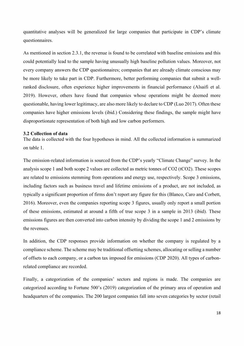
quantitative analyses will be generalized for large companies that participate in CDP’s climatequestionnaires.As mentioned in section 2.3.1, the revenue is found to be correlated with baseline emissions and thiscould potentially lead to the sample having unusually high baseline pollution values. Moreover, notevery company answers the CDP questionnaires; companies that are already climate conscious maybe more likely to take part in CDP. Furthermore, better performing companies that submit a well-ranked disclosure, often experience higher improvements in financial performance (Alsaifi et al.2019). However, others have found that companies whose operations might be deemed morequestionable, having lower legitimacy, are also more likely to declare to CDP (Luo 2017). Often thesecompanies have higher emissions levels (ibid.) Considering these findings, the sample might havedisproportionate representation of both high and low carbon performers.3.2 Collection of dataThe data is collected with the four hypotheses in mind. All the collected information is summarizedon table 1.The emission-related information is sourced from the CDP’s yearly “Climate Change” survey. In theanalysis scope 1 and both scope 2 values are collected as metric tonnes of CO2 (tCO2). These scopesare related to emissions stemming from operations and energy use, respectively. Scope 3 emissions,including factors such as business travel and lifetime emissions of a product, are not included, astypically a significant proportion of firms don’t report any figure for this (Blanco, Caro and Corbett,2016). Moreover, even the companies reporting scope 3 figures, usually only report a small portionof these emissions, estimated at around a fifth of true scope 3 in a sample in 2013 (ibid). Theseemissions figures are then converted into carbon intensity by dividing the scope 1 and 2 emissions bythe revenues.In addition, the CDP responses provide information on whether the company is regulated by acompliance scheme. The scheme may be traditional offsetting schemes, allocating or selling a numberof offsets to each company, or a carbon tax imposed for emissions (CDP 2020). All types of carbon-related compliance are recorded.Finally, a categorization of the companies’ sectors and regions is made. The companies arecategorized according to Fortune 500’s (2019) categorization of the primary area of operation andheadquarters of the companies. The 200 largest companies fall into seven categories by sector (retail

19

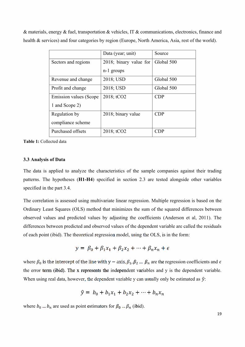
& materials, energy & fuel, transportation & vehicles, IT & communications, electronics, finance andhealth & services) and four categories by region (Europe, North America, Asia, rest of the world).

Data (year; unit) SourceSectors and regions 2018; binary value for

n-1 groupsGlobal 500

Revenue and change 2018; USD Global 500Profit and change 2018; USD Global 500Emission values (Scope1 and Scope 2)

2018; tCO2 CDP

Regulation bycompliance scheme

2018; binary value CDP

Purchased offsets 2018; tCO2 CDPTable 1: Collected data

3.3 Analysis of DataThe data is applied to analyze the characteristics of the sample companies against their tradingpatterns. The hypotheses (H1-H4) specified in section 2.3 are tested alongside other variablesspecified in the part 3.4.The correlation is assessed using multivariate linear regression. Multiple regression is based on theOrdinary Least Squares (OLS) method that minimizes the sum of the squared differences betweenobserved values and predicted values by adjusting the coefficients (Anderson et al, 2011). Thedifferences between predicted and observed values of the dependent variable are called the residualsof each point (ibid). The theoretical regression model, using the OLS, is in the form:

𝑦 𝛽0 𝛽1𝑥1 𝛽2𝑥2 ⋯ 𝛽𝑛𝑥𝑛 𝜖

where 𝛽0 − 𝛽1 𝛽2 𝛽𝑛 are the regression coefficients and 𝜖

the error term (ibid). The x represents the independent variables and y is the dependent variable.When using real data, however, the dependent variable y can usually only be estimated as 𝑦:

𝑦 𝑏0 𝑏1𝑥1 𝑏2𝑥2 ⋯ 𝑏𝑛𝑥𝑛

where 𝑏0 𝑏𝑛 are used as point estimators for 𝛽0 𝛽𝑛 (ibid).

20

The error term in the regression model represents the portion of y that the model does not predict(Fox 2016). A larger residual can signal a lower predicting value of the model. Indeed, themeasurement for the proportion of the variability that the regression model estimates, called themultiple coefficient of determination or R-squared, uses the sum of individual error squares(Anderson et al. 2011). The formula is as follows:

𝑅2 ∑ 𝑦𝑖 − 𝑦 2

∑ 𝑦𝑖 − 𝑦 2 ∑ 𝑦𝑖 − 𝑦𝑖2

where 𝑦𝑖 is the predicted value at 𝑥𝑖, 𝑦𝑖 is the actual value at 𝑥𝑖 and 𝑦 is the mean value of y (ibid).As seen from the equation, increase in the sum of squared residuals, ∑ 𝑦𝑖 − 𝑦𝑖

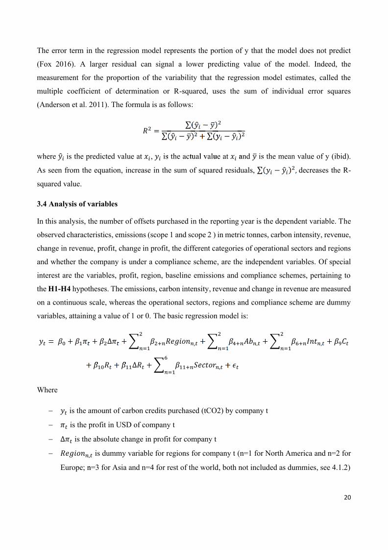
2 decreases the R-squared value.3.4 Analysis of variablesIn this analysis, the number of offsets purchased in the reporting year is the dependent variable. Theobserved characteristics, emissions (scope 1 and scope 2 ) in metric tonnes, carbon intensity, revenue,change in revenue, profit, change in profit, the different categories of operational sectors and regionsand whether the company is under a compliance scheme, are the independent variables. Of specialinterest are the variables, profit, region, baseline emissions and compliance schemes, pertaining tothe H1-H4 hypotheses. The emissions, carbon intensity, revenue and change in revenue are measuredon a continuous scale, whereas the operational sectors, regions and compliance scheme are dummyvariables, attaining a value of 1 or 0. The basic regression model is:𝑦𝑡 𝛽0 𝛽1𝜋𝑡 𝛽2∆𝜋𝑡 𝛽2+𝑛𝑅𝑒𝑔𝑖𝑜𝑛𝑛 𝑡

2

𝑛=1𝛽4+𝑛𝐴𝑏𝑛 𝑡

2

𝑛=1𝛽 +𝑛𝐼𝑛𝑡𝑛 𝑡

2

𝑛=1𝛽9𝐶𝑡

𝛽10𝑅𝑡 𝛽11∆𝑅𝑡 𝛽11+𝑛𝑆𝑒𝑐𝑡𝑜𝑟𝑛 𝑡𝑛=1

𝜖𝑡

Where 𝑦𝑡 is the amount of carbon credits purchased (tCO2) by company t 𝜋𝑡 is the profit in USD of company t ∆𝜋𝑡 is the absolute change in profit for company t 𝑅𝑒𝑔𝑖𝑜𝑛𝑛 𝑡 is dummy variable for regions for company t (n=1 for North America and n=2 for

Europe; n=3 for Asia and n=4 for rest of the world, both not included as dummies, see 4.1.2)

21

𝐴𝑏𝑛 𝑡 is the absolute baseline emissions in tCO2 for company t (n=1 for combined scope 1and 2, n=2 for scope 2)

𝐼𝑛𝑡𝑛 𝑡 is the carbon intensity for company t (n=1 for combined scope 1 and scope 2, n=2 forscope 2)

𝐶𝑡 is dummy variable for compliance scheme for company t 𝑅𝑡 is the revenue in USD for company t ∆𝑅𝑡 is the absolute change in revenue for company t 𝑆𝑒𝑐𝑡𝑜𝑟𝑛 𝑡 is the sector dummy for company t (t=1 for retail and materials, t=2 for energy and

fuel, t=3 for transportation and vehicles, t=4 for IT and communications, t=5 for electronics,t=6 for finance, t=7 for health and services that is not included as a dummy)

𝜖𝑡 is the error term for company tHowever, depending on the suitability and strength of the model two changes are considered:logarithmic transformation and changing the dependent variable into binary form. In the latter case,the model attempts to estimate what characteristics are connected to whether companies purchasecarbon credits or not whereas the original, non-binary model looks at how many credits companiespurchase.3.5 OLS AssumptionsTo assess the fit of the linear regression model, the fulfillment of OLS assumptions is analyzed. Theseassumptions ensure that the model is suitable and representable. There are seven commonly statedassumptions, however, different authors choose to put more emphasis on some of them than others.According to Osborne and Waters (2002), four of the assumptions can be controlled by proper studydesign and analysis: linearity, normality, reliability of data and homoscedasticity. In addition,Anderson et al. (2011) highlights two properties of the error term: expected value of zero and no serialcorrelation between error terms. Serial correlation will not be considered as it is more relevant intime-series analyses. Finally, Fox (2016) and Anderson et al. (2011) bring up multicollinearity.All in all, in this paper the following assumptions are considered: linearity, normality of residuals,reliability of data, homoscedasticity, expected value of error term and multicollinearity.3.5.1 LinearityThe independent variables should have a linear relationship with the dependent variable, bothcollectively and individually (Fox 2016). If one independent variable, for example, lacks a linear

22

relationship with the dependent variable, the regression model may underestimate the relationship(Osborne and Waters 2002). On the other hand, the other independent variables might experience atype I error of overestimation if they correlate with the independent variable (ibid). All independentvariables, except for the dummy variables, should therefore be assessed for linearity. The method ofassessment is described in section 4.2.1.3.5.2 Normality of ResidualsAlthough not a requirement of OLS analysis per se, normality of residuals is relevant when testing ahypothesis using a linear regression, because non-standardly distributed residuals can impact themean and interpretative value of the regression model (Fox 2016). Non-standard distribution can beapparent as skewness and kurtosis of the distribution curve of the residuals. Skewness describes theshape of the distribution, where any value other than zero shows that the distribution is asymmetrical(Anderson et al. 2011). When, for example, skewness is negative the distribution has a longer tail onthe left. In this case, the mean of the residuals will be less than the median (ibid). Kurtosis relates tothe heaviness or thinness of the tails of the distribution (NIST/SEMATECH 2013). Thicker tails, asign of more outliers, result in kurtosis value of more than the expected value of three (ibid).3.5.3 ExogeneityThere are many reasons why data might not be reliable from selection of inadequate sources to thevariables not being exogenous. Endogeneity may render the independent variables correlated withthe error term: denoting the erroneous observation of x as 𝑥 𝑥 𝑢 and holding other assumptionsconstant, a simplified single-variable regression model becomes 𝑦 𝛽 𝑥 − 𝑢 𝜖 𝛽𝑥 𝜖 −

𝛽𝑢 (Pischke 2007). If this sort of endogeneity is present, adding an instrumental variable can resolvethe correlation (Fox 2016).3.5.4 HomoscedasticityThe fourth assumption of homoscedasticity states that the residuals of the independent variablesshould have the same variance (Osborne and Waters 2002). Lack of homoscedasticity can make theOLS model less efficient and affect the standard error coefficient (Fox 2016). The White’s test iscommonly used to check for homoscedasticity (Baum 2006). In addition, often a graphical assessmentis useful because the White’s test is sensitive to OLS model assumptions and could exaggerate theheteroscedasticity (ULibraries Research Guides - Regression Diagnostics, 2020).3.5.5 Expected Value of the Error TermMoreover, the model assumes that the expected value of 𝜖 is zero 𝐸 𝜖 , implying that

23

𝐸 𝑦 𝛽0 𝛽1𝑥1 𝛽2𝑥2 ⋯ 𝛽𝑛𝑥𝑛 (Anderson et al, 2011). However, a non-zero mean of theerror term will only affect the regression constant and not the actual coefficients (Hong 2016).Denoting 𝐸 𝜖 𝑐 𝜖 𝑐 𝜇 , where 𝜇 is the error term with expected value of zero, theequation becomes 𝑦 𝛽0 𝑐 𝛽1𝑥1 𝛽2𝑥2 ⋯ 𝛽𝑛𝑥𝑛 𝜇 (ibid.).3.5.6 Lack of MulticollinearityMulticollinearity refers to linear or almost linear relationship between two or more of the independentvariables (Fox 2016). High correlation between independent variables makes the interpretation of thedistinct effects of the variables difficult (Anderson et al. 2011). The estimated coefficients canbecome unreliable and standard errors overestimated (ULibraries Research Guides - RegressionDiagnostics, 2020).If the correlation is outside the range [-0.70 ;0.70], for any two independent variables, one of thevariables is dropped or adjusted (Anderson et al 2011). For example, Goldhammer’s et al. (2016)research found significant correlation between the revenues and absolute baseline emission values,the higher estimations exceeding the limits for. Therefore, these two variables might also exhibitcorrelation in this study, requiring the removal of the emission variable.

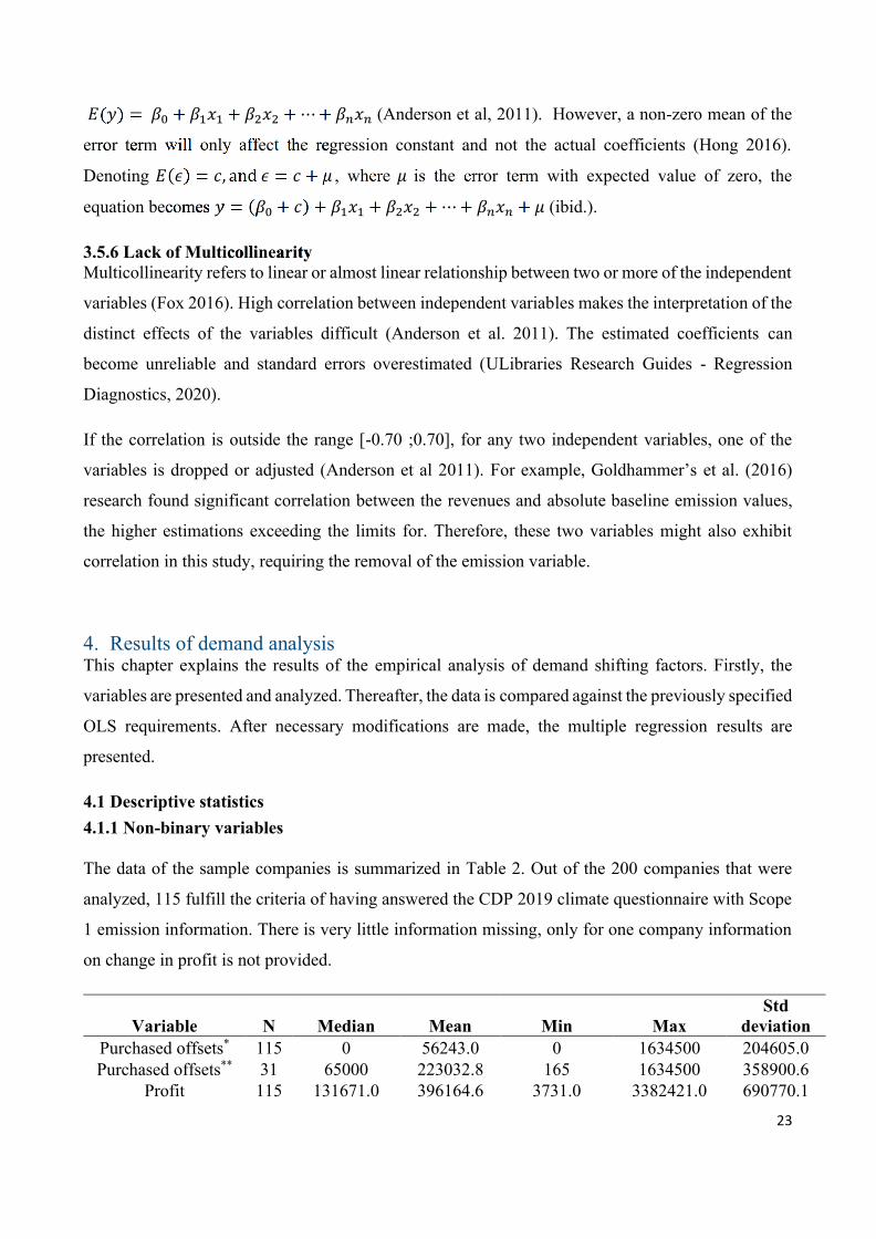
4. Results of demand analysisThis chapter explains the results of the empirical analysis of demand shifting factors. Firstly, thevariables are presented and analyzed. Thereafter, the data is compared against the previously specifiedOLS requirements. After necessary modifications are made, the multiple regression results arepresented.4.1 Descriptive statistics4.1.1 Non-binary variablesThe data of the sample companies is summarized in Table 2. Out of the 200 companies that wereanalyzed, 115 fulfill the criteria of having answered the CDP 2019 climate questionnaire with Scope1 emission information. There is very little information missing, only for one company informationon change in profit is not provided. A

Variable N Median Mean Min Max StddeviationPurchased offsets* 115 0 56243.0 0 1634500 204605.0Purchased offsets** 31 65000 223032.8 165 1634500 358900.6Profit 115 131671.0 396164.6 3731.0 3382421.0 690770.1

24

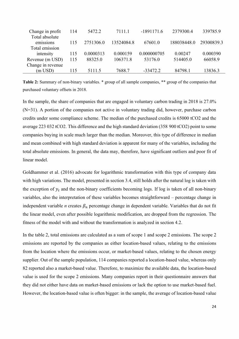
Change in profit 114 5472.2 7111.1 -1891171.6 2379300.4 339785.9Total absoluteemissions 115 2751306.0 13524084.8 67601.0 188038448.0 29300839.3Total emissionintensity 115 0.0000313 0.000159 0.000000705 0.00247 0.000390Revenue (m USD) 115 88325.0 106371.8 53176.0 514405.0 66058.9Change in revenue(m USD) 115 5111.5 7688.7 -33472.2 84798.1 13836.3Table 2: Summary of non-binary variables. * group of all sample companies, ** group of the companies thatpurchased voluntary offsets in 2018.In the sample, the share of companies that are engaged in voluntary carbon trading in 2018 is 27.0%(N=31). A portion of the companies not active in voluntary trading did, however, purchase carboncredits under some compliance scheme. The median of the purchased credits is 65000 tCO2 and theaverage 223 032 tCO2. This difference and the high standard deviation (358 900 tCO2) point to somecompanies buying in scale much larger than the median. Moreover, this type of difference in medianand mean combined with high standard deviation is apparent for many of the variables, including thetotal absolute emissions. In general, the data may, therefore, have significant outliers and poor fit oflinear model.Goldhammer et al. (2016) advocate for logarithmic transformation with this type of company datawith high variations. The model, presented in section 3.4, still holds after the natural log is taken withthe exception of 𝑦𝑡 and the non-binary coefficients becoming logs. If log is taken of all non-binaryvariables, also the interpretation of these variables becomes straightforward – percentage change inindependent variable n creates 𝛽𝑛 percentage change in dependent variable. Variables that do not fitthe linear model, even after possible logarithmic modification, are dropped from the regression. Thefitness of the model with and without the transformation is analyzed in section 4.2.In the table 2, total emissions are calculated as a sum of scope 1 and scope 2 emissions. The scope 2emissions are reported by the companies as either location-based values, relating to the emissionsfrom the location where the emissions occur, or market-based values, relating to the chosen energysupplier. Out of the sample population, 114 companies reported a location-based value, whereas only82 reported also a market-based value. Therefore, to maximize the available data, the location-basedvalue is used for the scope 2 emissions. Many companies report in their questionnaire answers thatthey did not either have data on market-based emissions or lack the option to use market-based fuel.However, the location-based value is often bigger: in the sample, the average of location-based value

25

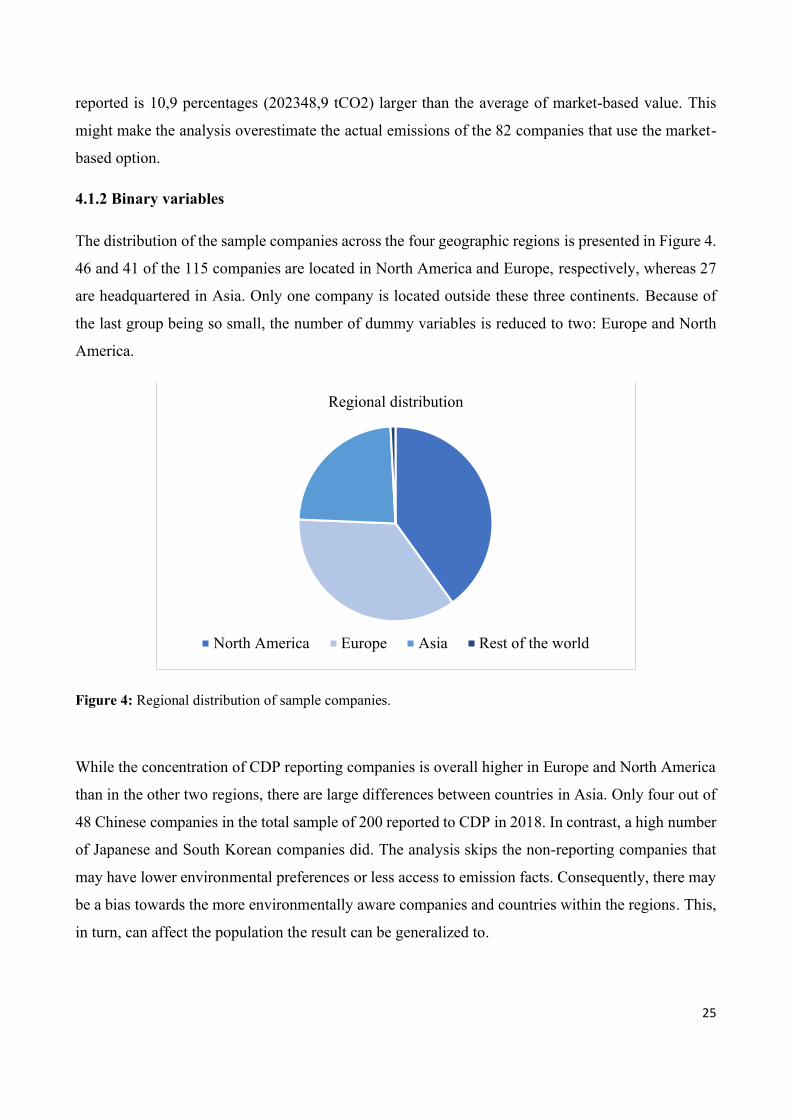
reported is 10,9 percentages (202348,9 tCO2) larger than the average of market-based value. Thismight make the analysis overestimate the actual emissions of the 82 companies that use the market-based option.4.1.2 Binary variablesThe distribution of the sample companies across the four geographic regions is presented in Figure 4.46 and 41 of the 115 companies are located in North America and Europe, respectively, whereas 27are headquartered in Asia. Only one company is located outside these three continents. Because ofthe last group being so small, the number of dummy variables is reduced to two: Europe and NorthAmerica.

Figure 4: Regional distribution of sample companies.

While the concentration of CDP reporting companies is overall higher in Europe and North Americathan in the other two regions, there are large differences between countries in Asia. Only four out of48 Chinese companies in the total sample of 200 reported to CDP in 2018. In contrast, a high numberof Japanese and South Korean companies did. The analysis skips the non-reporting companies thatmay have lower environmental preferences or less access to emission facts. Consequently, there maybe a bias towards the more environmentally aware companies and countries within the regions. This,in turn, can affect the population the result can be generalized to.

Regional distribution

North America Europe Asia Rest of the world

26

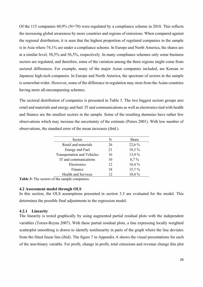
Of the 115 companies 60,9% (N=70) were regulated by a compliance scheme in 2018. This reflectsthe increasing global awareness by more countries and regions of emissions. When compared againstthe regional distribution, it is seen that the highest proportion of regulated companies in the sampleis in Asia where 74,1% are under a compliance scheme. In Europe and North America, the shares areat a similar level, 58,5% and 56,5%, respectively. In many compliance schemes only some businesssectors are regulated, and therefore, some of the variation among the three regions might come fromsectoral differences. For example, many of the major Asian companies included, are Korean orJapanese high-tech companies. In Europe and North America, the spectrum of sectors in the sampleis somewhat wider. However, some of the difference in regulation may stem from the Asian countrieshaving more all-encompassing schemes.The sectoral distribution of companies is presented in Table 3. The two biggest sectors groups arreretail and materials and energy and fuel. IT and communications as well as electronics tied with healthand finance are the smallest sectors in the sample. Some of the resulting dummies have rather fewobservations which may increase the uncertainty of the estimate (Peters 2001). With low number ofobservations, the standard error of the mean increases (ibid.).

Sector N ShareRetail and materials 26 22,6 %Energy and Fuel 21 18,3 %Transportation and Vehicles 16 13,9 %IT and communications 10 8,7 %Electronics 12 10,4 %Finance 18 15,7 %Health and Services 12 10,4 %Table 3: The sectors of the sample companies.

4.2 Assessment model through OLSIn this section, the OLS assumptions presented in section 3.5 are evaluated for the model. Thisdetermines the possible final adjustments to the regression model.4.2.1 LinearityThe linearity is tested graphically by using augmented partial residual plots with the independentvariables (Torres-Reyna 2007). With these partial residual plots, a line expressing locally weightedscatterplot smoothing is drawn to identify nonlinearity in parts of the graph where the line deviatesfrom the fitted linear line (ibid). The figure 7 in Appendix A shows the visual presentations for eachof the non-binary variable. For profit, change in profit, total emissions and revenue change this plot

27

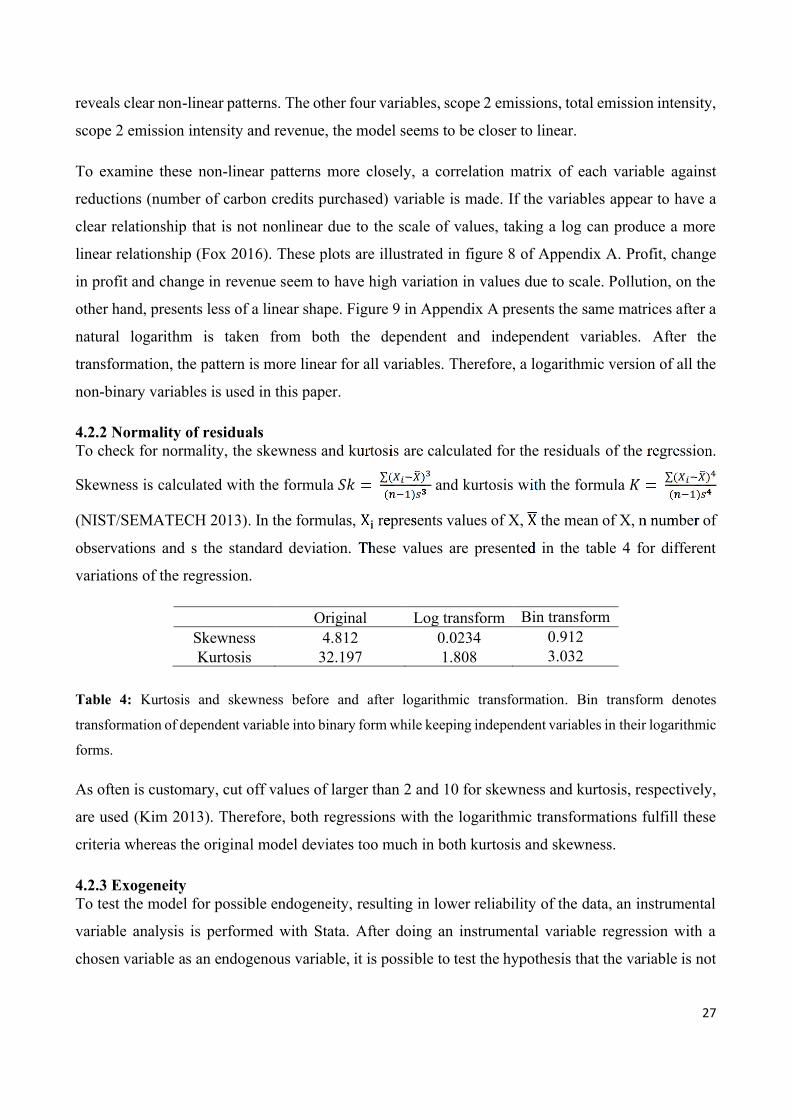
reveals clear non-linear patterns. The other four variables, scope 2 emissions, total emission intensity,scope 2 emission intensity and revenue, the model seems to be closer to linear.To examine these non-linear patterns more closely, a correlation matrix of each variable againstreductions (number of carbon credits purchased) variable is made. If the variables appear to have aclear relationship that is not nonlinear due to the scale of values, taking a log can produce a morelinear relationship (Fox 2016). These plots are illustrated in figure 8 of Appendix A. Profit, changein profit and change in revenue seem to have high variation in values due to scale. Pollution, on theother hand, presents less of a linear shape. Figure 9 in Appendix A presents the same matrices after anatural logarithm is taken from both the dependent and independent variables. After thetransformation, the pattern is more linear for all variables. Therefore, a logarithmic version of all thenon-binary variables is used in this paper.4.2.2 Normality of residualsTo check for normality, the skewness and kurtosis are calculated for the residuals of the regression.Skewness is calculated with the formula 𝑆𝑘 ∑ 𝑖− 3

𝑛−1 3 and kurtosis with the formula 𝐾 ∑ 𝑖− 4

𝑛−1 4

(NIST/SEMATECH 2013). In the formulas, i represents values of X, the mean of X, n number ofobservations and s the standard deviation. These values are presented in the table 4 for differentvariations of the regression.

Original Log transform Bin transformSkewness 4.812 0.0234 0.912Kurtosis 32.197 1.808 3.032Table 4: Kurtosis and skewness before and after logarithmic transformation. Bin transform denotestransformation of dependent variable into binary form while keeping independent variables in their logarithmicforms.As often is customary, cut off values of larger than 2 and 10 for skewness and kurtosis, respectively,are used (Kim 2013). Therefore, both regressions with the logarithmic transformations fulfill thesecriteria whereas the original model deviates too much in both kurtosis and skewness.4.2.3 ExogeneityTo test the model for possible endogeneity, resulting in lower reliability of the data, an instrumentalvariable analysis is performed with Stata. After doing an instrumental variable regression with achosen variable as an endogenous variable, it is possible to test the hypothesis that the variable is not

28

endogenous. In the data, all of the variables have high p-values, between 0,16 and 0,79, showing noendogeneity.4.2.4 HomoscedasticityThe White’s test that the null hypothesis of homoscedasticity holds (p-value > 0,05). Therefore, thereis no need for graphical analysis that is often less biased towards heteroskedasticity (ULibrariesResearch Guides - Regression Diagnostics, 2020).4.2.5 Expected value of error termThis error term value assumption can be checked by graphing the residuals against the fitted values,the same way as with homoscedasticity if White’s test has a low p-value. The graph should displaysymmetry of the residual values around zero. The figure 10 in Appendix B represents the residualplots for regressions with and without a logarithmic transformation. The residuals have a moreconstant variance after the transformation, further supporting the choice.4.2.6. Lack of multicollinearityAs concluded earlier, the acceptable limit for collinearity between any two independent variables isbetween -0.7 and 0.7. Table 7 in the Appendix C shows the correlation matrix of all variables. Unlikefound by Goldhammer et al. (2016), there is no relevant correlation between baseline emissions andrevenue. However, two significant correlations are present: total emissions and total emissionsintensity; scope 2 emissions and scope 2 intensity. To overcome this problem that may otherwiseweaken the model, total emissions and scope 2 emissions are removed. This is to preserve thehypothesis 3 of baseline emissions. As Lewandowski (2017) analyzes, intensity is a more comparableway of assessing emissions and, therefore, the absolute total emissions are chosen to be removed.4.2.7 Adjusted regression modelConsidering these assumptions, the resulting model is a logarithmic transformation with the twovariables removed due to multicollinearity. This ensures a more reliable and fitting analysis. Theformula is as follows:

𝑦𝑡 𝛽0 𝛽1 𝜋𝑡 𝛽2 ∆𝜋𝑡 𝛽2+𝑛𝑅𝑒𝑔𝑖𝑜𝑛𝑛 𝑡

2

𝑛=1𝛽4+𝑛𝐼𝑛𝑡𝑛 𝑡

2

𝑛=1𝛽7𝐶𝑡

𝛽8 𝑅𝑡 𝛽9 ∆𝑅𝑡 𝛽9+𝑛𝑆𝑒𝑐𝑡𝑜𝑟𝑛 𝑡𝑛=1

𝜖𝑡

In the model, log denotes natural a logarithm, while otherwise same definitions as specified in section3.4 hold. Because most companies had not purchased any offsets A modification is made to include

29

companies with zero reductions through carbon credits: zero is changed to 0.01 to allow for a logvalue to exist. Additionally, the regression is run with a binary form of 𝑦𝑡 where 0 signifies nopurchases whereas 1 covers all companies purchasing carbon credits.4.3 Regression resultsThe table 5 shows the results of the two regression analysis cases: (1) with the logarithmictransformation of the reductions variable and (2) with the dummy form of the variable. Overall, theR-squared and the adjusted R-squared are on the lower side, partly due to the many differences withinthe sample and low volume of companies actively buying credits. Moreover, the R-squared is somehigher for the binary model: 0.362 compared to 0.331 in the logarithmic model. Yet, both the R-values show some explanatory power, and even after the adjustment the models are estimated toexplain 22.9% (1) and 26.4% (2) of the variations in the dependent variables. The standard errors arenotably higher in the logarithmic model, indicating a lower accuracy of the predictions than in thebinary model.

(1) (2)Log(reductions) Bin(reductions)Log(profit) -7.375 -0.489(9.431) (0.995)Log(pchange) 2.236** 0.183**(0.974) (0.081)Europe 1.974 0.118*(1.618) (0.136)US 1.623 0.0997(1.312) (0.104)Log(inttotal) -2002.8 -114.7(0.703) (0.059)Log(int2) 0.369 0.0313(0 .493) (0.039)Compliance 0.919 0.115***(0.792) (0.043)Log(revenue) -1.529 -0.0836(1.964) (0.152)Log(Revenuechange) 11.368** 0.983**(5.010) (0.257)Oil -3.756 -0.261(3.402) (0.239)Retail -4.990** -0.360**(2.453) (0.1702)Transport -2.577 -0.204(3.017) (0.206)

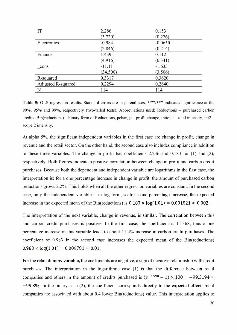
30

IT 2.286 0.153(3.720) (0.276)Electronics -0.984 -0.0650(2.846) (0.214)Finance 1.439 0.112(4.916) (0.341)_cons -11.11 -1.633(34.500) (3.506)R-squared 0.3317 0.3620Adjusted R-squared 0.2294 0.2640N 114 114Table 5: OLS regression results. Standard errors are in parentheses. */**/*** indicates significance at the90%, 95% and 99%, respectively (two-tailed tests). Abbreviations used: Reductions – purchased carboncredits, Bin(reductions) – binary form of Reductions, pchange – profit change, inttotal – total intensity, int2 –scope 2 intensity.At alpha 5%, the significant independent variables in the first case are change in profit, change inrevenue and the retail sector. On the other hand, the second case also includes compliance in additionto these three variables. The change in profit has coefficients 2.236 and 0.183 for (1) and (2),respectively. Both figures indicate a positive correlation between change in profit and carbon creditpurchases. Because both the dependent and independent variable are logarithms in the first case, theinterpretation is: for a one percentage increase in change in profit, the amount of purchased carbonreductions grows 2.2%. This holds when all the other regression variables are constant. In the secondcase, only the independent variable is in log form, so for a one percentage increase, the expectedincrease in the expected mean of the Bin(reductions) is ≈ .The interpretation of the next variable, change in revenue, is similar. The correlation between thisand carbon credit purchases is positive. In the first case, the coefficient is 11.368, thus a onepercentage increase in this variable leads to about 11.4% increase in carbon credit purchases. Thecoefficient of 0.983 in the second case increases the expected mean of the Bin(reductions)

≈ .For the retail dummy variable, the coefficients are negative, a sign of negative relationship with creditpurchases. The interpretation in the logarithmic case (1) is that the difference between retailcompanies and others in the amount of credits purchased is 𝑒−4 990 − − ≈

− . In the binary case (2), the coefficient corresponds directly to the expected effect: retailcompanies are associated with about 0.4 lower Bin(reductions) value. This interpretation applies to

31

the compliance dummy in the binary case as well, although the correlation is now positive. Thecompanies under a compliance scheme have an estimated 0.1 higher Bin(reductions) value. Thesignificant results are summarized in table 6.

Log(reductions) Bin(reductions)Change in profit positive positiveChange in revenue positive positiveRetail negative negativeCompliance n/a positiveTable 6: Summary of results.5. The demand and supply modelIn this chapter, firstly, the findings of the quantitative demand analysis are discussed in relation to theliterature review’s model. Then, the supply side model is assessed, using pricing data. Theimplications of the findings and conclusion are finally presented in the next chapter.5.1 Demand modelThe regression model is found to not completely account for the factors affecting the offset purchasesof the sample companies. This can be due to some significant factors missing from the model, andthese missing variables can then shift the demand curve. However, the analysis supports two of thefour hypotheses of the literature review. In addition, two other suggested shifters are found.The hypothesis 1 – profits or change in profits being positively correlated with the amount of carboncredits a company purchases – is supported by both regression cases. While the profits are notsignificantly correlated, the changes in them are. This reflects that the profit grows more as companiesbuy more credits or switch from being non-buyers to buyers. It may be that companies experiencinghighly increasing profits are more willing to buy carbon credits. Alternatively, the purchasesthemselves may be fueling these increases in profits. In any case, the result indicates that the amountof profit increase and carbon purchases are positively linked. The effect size of the connection mightbe somewhat weakened by the model not grouping the companies by their baseline emission levels,hypothesized as being relevant by, for example, Lewandowski (2017). However, that the correlationis positive could indicate a higher proportion of low polluters. This would be in line with Alsaifi etal. (2019) and Luo (2017) in that these companies may be more willing and likely to report to CDPand thus to appear in the sample population.In addition, the change in revenue has positive correlation with reductions in both cases. This furthersupports the theory that carbon offset purchases and financial gains are connected. The interpretation

32

of this result is that as revenues grow more, the companies tend to buy more offsets or be more likelyto buy their first offset.In addition, the fourth hypothesis on the impact of being regulated by a compliance scheme is backedby the binary regression model. The coefficient of this variable in the binary model is about 50 timesgreater in strength than that of change in profit. However, as the variables are not standardized, thecoefficient sizes might not be comparable. Also, the direction of the effect was not clear from theliterature review. This analysis shows a positive correlation for this variable and reductions throughcarbon credits. In other words, as companies become regulated compliance schemes, they becomemore likely to also buy voluntary offsets. Perhaps this effect is an extension of the pre-compliancehump. Yet, the hump is usually defined as a temporary change in response to regulatory pressuresand threats (Donofrio et al. 2019; Zhao et al. 2018). It might be that companies that are alreadyexperiencing some financial repercussions of their emissions are more actively preparing for newregulations by investing in carbon reductions.The hypotheses 2 and 3 are not supported by the data. The hypothesis 2 is that baseline emissionintensities are negatively correlated with carbon credit purchases. While not significant according top-values, the variable total intensity has indeed negative coefficients. Yet, there might be too muchvariability in the data to establish a significant connection, or some non-linear pattern.The hypothesis 3, of Europe and North America having positive correlation to the offset purchases,would only be supported for Europe if one-tailed test was used in the binary model. The coefficientsare in all cases positive as speculated. However, the p-values may have been weakened by the databeing very concentrated to these regions: 76% of the 115 sample were headquartered in these two.Moreover, as discussed in 4.1.2, the Asian values may have a bias towards non-Chinese companiesand thus exhibiting a pattern more similar to Europe and North America (Lee et al. 2015). The fourthregion is insignificant for the results as only one company is in it.All in all, the regression analysis serves to analyze some of the factors affecting the demand of carboncredits among some of the largest companies. As mentioned in section 2.3.2, the customer andcompany preferences are not included in the analysis, although they might be significant. The fourfactors identified in this study to correlate with reductions can be included as demand shifting factorsin the model. Out of the variables, growing profit and revenue as well as regulation would shift thedemand to the right, and being a retail company would cause a shift to the left. Considering that the

33

demand is theorized to be rather inelastic (Spiekermann 2013), changes in price within some rangemight have lesser of an impact on the demanded quantity than the demand shifters.5.2 Supply modelAs discussed in section 2.4, the supply trends of carbon credits might be somewhat different, basedon the category of the project. However, all the categories experience some level of lag in the time ittook for the credits to be sold after issuance (Hamrick and Gallant 2017).A general model of supply assumes that more producers are willing to put out projects at higher pricesthan at lower levels (OpenStax Economics 2016). Inverse is assumed to hold for demand in general(ibid.). As the demand is not always easy to predict (Borden 2020), it is not surprising that the supplydoes not always meet the demand at the equilibrium point. This is supported by the findings ofHamrick and Gallant (2017): out of all the produced offsets in 2016, 47% did not sell that year. Yetsome categories experience more significant lag than others. Projects in the categories forestry andwaste sold 74% and 80% of their credits by end of the year, respectively, whereas the other categoriesall sold fewer that half of their credits (ibid.).The reasons behind this lag might be in the price levels: most producers interviewed stated that theydid not find an appropriate buyer or decided to wait for better market prices (ibid.). The pricesexpected by these suppliers are not provided, but as mentioned, the price level of voluntary marketsis currently less than that of the compliance market. There are multiple ways of calculating a suitableprice for the offsets from the producer perspective, with some methods considering only the necessaryproduction costs and some also other factors, such as the social value delivered (The Gold Standard2020b). The “Fairtrade Minimum Price” considers the operational and transaction costs of the projectas well as a business margin of about 5-10% of the credit price (ibid.). Both the actual price levelsand the minimum price estimates vary significantly among the project categories. For each category,yearly mean prices and sold quantities (tCO2) are provided in the Ecosystem Marketplace’s “State ofthe Voluntary Carbon Markets” publications, such as those by Donofrio et al. (2019; 2020) andHamrick and Gallant (2017). For example, according to these sources, land use and forestry projectshave minimum price quoted at 12.4 USD and yearly mean prices between 3 and 5 USD and forrenewable energy the same estimates are 7.3 USD and 1-2 USD, respectively.This situation is depicted theoretically in figure 5, according to the model of demand and supply bySpiekermann (2013), The “Fairtrade Minimum Price” is denoted as p1 and the supplied quantity atthis price level as 1. When this price is above the equilibrium price (q*, p*), the demand curve

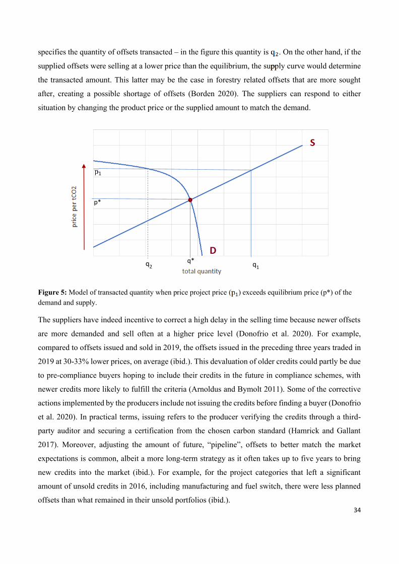
34

specifies the quantity of offsets transacted – in the figure this quantity is 2. On the other hand, if thesupplied offsets were selling at a lower price than the equilibrium, the supply curve would determinethe transacted amount. This latter may be the case in forestry related offsets that are more soughtafter, creating a possible shortage of offsets (Borden 2020). The suppliers can respond to eithersituation by changing the product price or the supplied amount to match the demand.

Figure 5: Model of transacted quantity when price project price ( 1) exceeds equilibrium price (p*) of thedemand and supply.The suppliers have indeed incentive to correct a high delay in the selling time because newer offsetsare more demanded and sell often at a higher price level (Donofrio et al. 2020). For example,compared to offsets issued and sold in 2019, the offsets issued in the preceding three years traded in2019 at 30-33% lower prices, on average (ibid.). This devaluation of older credits could partly be dueto pre-compliance buyers hoping to include their credits in the future in compliance schemes, withnewer credits more likely to fulfill the criteria (Arnoldus and Bymolt 2011). Some of the correctiveactions implemented by the producers include not issuing the credits before finding a buyer (Donofrioet al. 2020). In practical terms, issuing refers to the producer verifying the credits through a third-party auditor and securing a certification from the chosen carbon standard (Hamrick and Gallant2017). Moreover, adjusting the amount of future, “pipeline”, offsets to better match the marketexpectations is common, albeit a more long-term strategy as it often takes up to five years to bringnew credits into the market (ibid.). For example, for the project categories that left a significantamount of unsold credits in 2016, including manufacturing and fuel switch, there were less plannedoffsets than what remained in their unsold portfolios (ibid.).

q*q

q1

1

q2

p*q

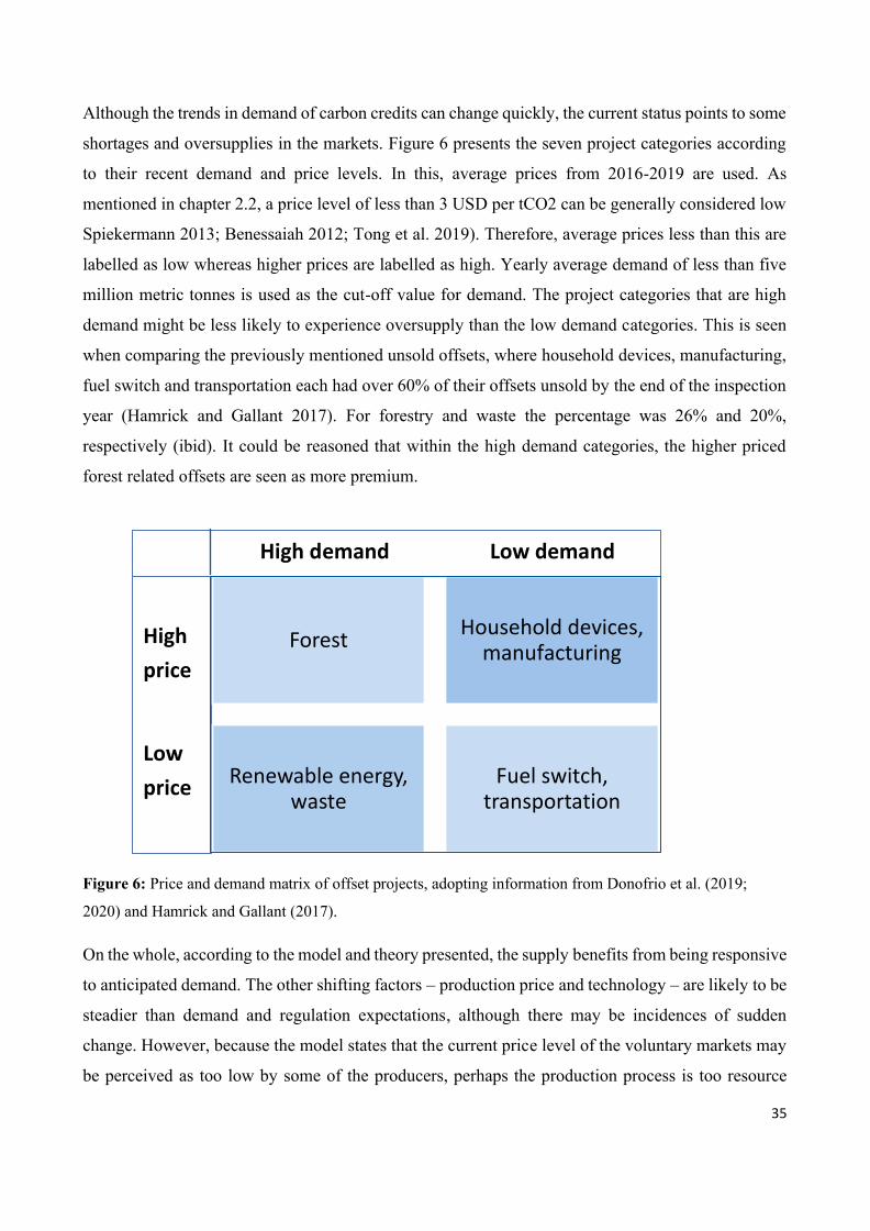
35

Although the trends in demand of carbon credits can change quickly, the current status points to someshortages and oversupplies in the markets. Figure 6 presents the seven project categories accordingto their recent demand and price levels. In this, average prices from 2016-2019 are used. Asmentioned in chapter 2.2, a price level of less than 3 USD per tCO2 can be generally considered lowSpiekermann 2013; Benessaiah 2012; Tong et al. 2019). Therefore, average prices less than this arelabelled as low whereas higher prices are labelled as high. Yearly average demand of less than fivemillion metric tonnes is used as the cut-off value for demand. The project categories that are highdemand might be less likely to experience oversupply than the low demand categories. This is seenwhen comparing the previously mentioned unsold offsets, where household devices, manufacturing,fuel switch and transportation each had over 60% of their offsets unsold by the end of the inspectionyear (Hamrick and Gallant 2017). For forestry and waste the percentage was 26% and 20%,respectively (ibid). It could be reasoned that within the high demand categories, the higher pricedforest related offsets are seen as more premium.

Figure 6: Price and demand matrix of offset projects, adopting information from Donofrio et al. (2019;2020) and Hamrick and Gallant (2017).On the whole, according to the model and theory presented, the supply benefits from being responsiveto anticipated demand. The other shifting factors – production price and technology – are likely to besteadier than demand and regulation expectations, although there may be incidences of suddenchange. However, because the model states that the current price level of the voluntary markets maybe perceived as too low by some of the producers, perhaps the production process is too resource

Highprice

Lowprice

Forest Household devices,manufacturing

Renewable energy,waste Fuel switch,transportation

High demand Low demand

36

heavy for certain project types. Yet, when it comes to forestry, renewable energy and waste offsets,the high demand could indicate a possibility for a price level increase, especially considering thesuggested inelasticity of the demand.6. Discussion and conclusionThis study examines the quantitative side of voluntary carbon trading. Previous research on emissionmarkets is mostly concentrated on the compliance markets where the demand is comprised oforganizations who are required to buy credits to meet their climate goals. However, a main sourcecited in this study by Spiekermann (2013) suggests a model of supply and demand that is distinct forthe voluntary markets.The first research question of the factors impacting the demand of carbon credits is examined usingdata of the carbon credit purchases of 200 major companies. This study conducts multiple regressionsand finds four significant variables: change in revenue and profit, being under compliance regulationand in retail sector. Increased population of these types of companies may shift the demand withinthat sample.The second research question of a suitable model for the demand and supply is not completely coveredwith the data. Some relevant demand shifters are left out of the model and the pricing informationdoes not specify the price expectations. However, a model where the demand is less elastic than thesupply is outlined. The demand is, within a range of prices, affected more by the shifting factors thanchanges in supply. On the other hand, the supply is possibly more affected by the demand that theshifters. Nonetheless, one of the main shifters of the supply is assumed to be future expectations,which are especially relevant as more and more regions are entering regulated carbon markets. Thisincreased regulation is already shown as the high percentage of the sample regulated by a compliancescheme. Yet, even through this shifting factor, the supply side is highly concerned with the demand,the unpredictability of which can cause excesses and shortages of carbon credits. This furtherhighlights the need for research on demand in the voluntary markets.Moreover, the suppliers may not always be content with the currently low price levels of the voluntarymarkets. Since the supply and demand models need to essentially be constructed individually for eachproject category, raising the price levels could be possible for some types of credits. An example ofthis are forest related projects, such as reforestation, afforestation and Redd+. Yet, with some of themore readily available project types, such as the energy related projects, the suppliers may not be able

37

to increase the prices considerably without the demand going over to the elastic side and starting todecrease quickly.Some of the min limitations of the quantitative study on demand factors relate to the sample selectionas discussed in the methodology chapter. The demand side results may be more relatable to companiesthat are already more climate aware than average because they are reporting to the CDP. In addition,their revenues are high which is found to correlate with other factors, such as baseline emissions.High baseline emissions lead to other issues, for example to the risk of low legitimacy. These largecompanies are also often familiar names within the general public which may require them to paymore attention to stakeholder – especially customer and media – relations. This can make them morelikely to adopt strategies, including voluntary carbon trading. Another important consideration is thatcompanies may have different methods and accuracies in reporting their figures, even though theyare typically audited before being submitted.Moreover, the quantitative study has some limitations in the processing of the data. Firstly, thevariables are not normalized which makes the interpretation of the effect sizes more difficult.Secondly, the data does not naturally fit a linear model for all variables, and therefore logarithmictransformations are performed. Instead, perhaps a non-linear model could have been more fitting andproduce more telling results. A larger sample could have allowed splitting the data and to pinpointsome features that only hold for a portion of the sample with specific features.Another limitation of this study, outside of the quantitative part, is the lack of literature on the possibleshifters for both the supply and demand sides. Often, the existing theories hold to an adjacent setting,such as other similar variables or the compliance market. For example, in the analysis of financialfactors and their importance to demand, the studies cited are not related to correlations of these factorswith carbon trading, but rather correlations of factors to various other climate actions. This makes theevaluation of the factors inductive and based highly on assumptions. As mentioned earlier, somesignificant shifting factors are not identified. The same may hold for supply, which may have a higherdegree of impact from shifters, some of which may not yet be identified in this study.As there is lack of quantitative studies on the voluntary trading, future studies could explore thesupply and demand with larger data sets and possibly more generalizable samples. The model ofsupply and demand for each project category could be investigated. In addition, the pricing in thevoluntary markets, though sometimes discussed in literature, could benefit from more quantification.Many parties are interested in clarifying the pricing of different credits and the factors involved in the

38

price setting (Donofrio et al. 2020). This might also be important with the advent of many complianceregulations.ReferencesAbdallah, T., Farhat, A., Diabat, A. and Kennedy, S., 2012. Green supply chains with carbon trading

and environmental sourcing: Formulation and life cycle assessment. Applied MathematicalModelling, 36(9), pp.4271-4285.

Aghion, P., Benabou, R., Martin, R. and Roulet, A., 2020. Environmental Preferences AndTechnological Choices: Is Market Competition Clean Or Dirty?. [ebook] London School ofEconomics - Centre for Economic Performance. Available at:<http://cep.lse.ac.uk/pubs/download/dp1684.pdf> [Accessed 30 November 2020].

Alsaifi, K., Elnahass, M. and Salama, A., 2019. Carbon disclosure and financial performance: UKenvironmental policy. Business Strategy and the Environment, 29(2), pp.711-726.

Anderson, D., Sweeney, D. and Williams, T., 2011. Statistics For Business And Economics. 11th ed.Mason: South-Western Cengage Learning, pp.102-107;561-655.

Arnoldus, M. and Bymolt, R., 2011. Demystifying Carbon Markets. Amsterdam: KIT.Baum, C., 2006. An Introduction To Modern Econometrics Using Stata. College Station, Tex.: Stata

Press, p.146.Benessaiah, K., 2012. Carbon and livelihoods in Post-Kyoto: Assessing voluntary carbon

markets. Ecological Economics, 77, pp.1-6.Blanco, C., Caro, F. and Corbett, C., 2016. The state of supply chain carbon footprinting: analysis of

CDP disclosures by US firms. Journal of Cleaner Production, 135, pp.1189-1197.Borden, M., 2020. Interview With Verra (VCS) By Venla Pirhonen.Busch, T. and Lewandowski, S., 2017. Corporate Carbon and Financial Performance: A Meta-

analysis. Journal of Industrial Ecology, 22(4), pp.745-759.Cacho, O., Lipper, L. and Moss, J., 2013. Transaction costs of carbon offset projects: A comparative

study. Ecological Economics, 88, pp.232-243.

39

Cao, X., Li, X. and Breeze, T., 2020. Quantifying the Carbon Sequestration Costs for Pinus elliottiiAfforestation Project of China Greenhouse Gases Voluntary Emission Reduction Program: ACase Study in Jiangxi Province. Forests, 11(9).

CDP, 2020. Home - CDP. [online] Available at: <https://www.cdp.net/en> [Accessed 10 November2020].

Conte, M. and Kotchen, M., 2010. Explaining the Price of Voluntary Carbon Offsets. Climate ChangeEconomics, 01(02), pp.93-111.

Dahlmann, F., Branicki, L. and Brammer, S., 2017. Managing Carbon Aspirations: The Influence ofCorporate Climate Change Targets on Environmental Performance. Journal of Business Ethics,158(1), pp.1-24.

Dohnalova, Z. and Zimola, B., 2013. Corporate stakeholder management. Procedia - Social andBehavioral Sciences, 110(2014), pp.879-886.

Donofrio, S., 2020. Voluntary Carbon And The Post-Pandemic Recovery. State of Voluntary CarbonMarkets. [online] Ecosystem Marketplace. Available at:<https://app.hubspot.com/documents/3298623/view/88656172?accessId=b01f32> [Accessed10 November 2020].

Donofrio, S., Maguire, P., Merry, W. and Zwick, S., 2019. Financing Emissions Reductions For TheFuture. State of the Voluntary Carbon Markets. [online] Ecosystem Marketplace. Available at:<https://app.hubspot.com/documents/3298623/view/63001900?accessId=eb4b1a> [Accessed10 November 2020].

Donofrio, S., Maguire, P., Zwick, S., Merry, W., Wildish, J. and Myers, K., 2020. The Only ConstantThing Is Change. State Of Voluntary Carbon Markets. [online] Ecosystem Marketplace.Available at:<https://app.hubspot.com/documents/3298623/view/101893633?accessId=bf5d12> [Accessed21 December 2020].

Du, S., Hu, L. and Song, M., 2016. Production optimization considering environmental performanceand preference in the cap-and-trade system. Journal of Cleaner Production, 112, pp.1600-1607.

EU Science Hub - European Commission. 2020. Global CO2 Emissions Continue To Rise But EUBucks Global Trend - EU Science Hub - European Commission. [online] Available at:

40

<https://ec.europa.eu/jrc/en/news/global-co2-emissions-continue-rise-eu-bucks-global-trend>[Accessed 3 November 2020].

Fortune. 2018. Global 500. [online] Available at: <https://fortune.com/global500/2018> [Accessed10 November 2020].

Fortune. 2019. Global 500. [online] Available at: <https://fortune.com/global500/2019> [Accessed10 November 2020].

Fortune. 2020. Methodology For Global 500. [online] Available at: <https://fortune.com/franchise-list-page/global-500-methodology-2020> [Accessed 10 November 2020].

Fox, J., 2016. Applied Regression Analysis And Generalized Linear Models. 3rd ed. Thousand Oaks:SAGE Publications, pp.65-102;301-400.

Galán-Valdivieso, F., Saraite-Sariene, L., Alonso-Cañadas, J. and Caba-Pérez, M., 2019. DoCorporate Carbon Policies Enhance Legitimacy? A Social Media Perspective. Sustainability,11(4), p.1161.

Ganda, F. and Milondzo, K., 2018. The Impact of Carbon Emissions on Corporate FinancialPerformance: Evidence from the South African Firms. Sustainability, 10(2398).

Goldhammer, B., Busse, C. and Busch, T., 2016. Estimating Corporate Carbon Footprints withExternally Available Data. Journal of Industrial Ecology, 21(5), pp.1165-1179.

The Gold Standard, 2020a. The Role Of Voluntary Carbon Offsetting In A Post-Paris World | TheGold Standard. [online] Available at: <https://www.goldstandard.org/blog-item/role-voluntary-carbon-offsetting-post-paris-world> [Accessed 21 December 2020].

The Gold Standard, 2020b. CARBON PRICING: What Is A Carbon Credit Worth? | The GoldStandard. [online] Available at: <https://www.goldstandard.org/blog-item/carbon-pricing-what-carbon-credit-worth> [Accessed 22 December 2020].

The Greenhouse Gas Protocol, 2015. Top Ten Questions About The Scope 2 Guidance. [online]Available at: <https://ghgprotocol.org/blog/top-ten-questions-about-scope-2-guidance>[Accessed 15 November 2020].

Hamrick, K. and Gallant, M., 2017. Unlocking Potential. State of the Voluntary Carbon Markets.Ecosystem Marketplace.

41

Hamrick, K. and Gallant, M., 2018. Voluntary Carbon Market Insights: 2018 Outlook And First-Quarter Trends. State of the Voluntary Carbon Markets. Ecosystem Marketplace.

Hamrick, K. and Goldstein, A., 2016. Raising Ambition. State of the Voluntary Carbon Markets.Ecosystem Marketplace.

Hermwille, L. and Kreibich, N., 2016. Identity Crisis? Voluntary Carbon Crediting And The ParisAgreement. Wuppertal: Wuppertal Institute for Climate, Environment and Energy.

Hong, X., 2016. Lecture 3: Simple Linear Regression. [ebook] Maryland: University of Maryland.Available at: <http://econweb.umd.edu/~hong/files/Lecture3.pdf> [Accessed 14 November2020].

Iizuka, K. and Tateishi, R., 2015. Estimation of CO2 Sequestration by the Forests in Japan byDiscriminating Precise Tree Age Category using Remote Sensing Techniques. Remote Sensing,7(11), pp.15082-15113.

Internal Revenue Service. 2020. Yearly Average Currency Exchange Rates. [online] Available at:<https://www.irs.gov/individuals/international-taxpayers/yearly-average-currency-exchange-rates> [Accessed 19 November 2020].

Kim, H., 2013. Statistical notes for clinical researchers: assessing normal distribution (2) usingskewness and kurtosis. Restorative Dentistry & Endodontics, 38(1), p.52.

Kountouris, Y., Makuch, Z. and Loch, F., 2014. Quantification And Evaluation Of The VoluntaryMarket's Co-Benefits. [online] International Carbon Reduction and Offset Alliance. Availableat: <https://icroa.wildapricot.org/resources/Documents/ICROA_ICL_Co-BenefitsReport_2014.pdf> [Accessed 20 November 2020].

Lee, T., Markowitz, E., Howe, P., Ko, C. and Leiserowitz, A., 2015. Predictors of public climatechange awareness and risk perception around the world. Nature Climate Change, 5(11),pp.1014–1020.

Lewandowski, S., 2017. Corporate Carbon and Financial Performance: The Role of EmissionReductions. Business Strategy and the Environment, 26(8), pp.1196-1211.

Luo, L., 2017. The influence of institutional contexts on the relationship between voluntary carbondisclosure and carbon emission performance. Accounting & Finance, 59(2), pp.1235-1264.

42

Ma, Y., Zhang, Q., Yin, Q. and Wang, B., 2019. The Influence of Top Managers on EnvironmentalInformation Disclosure: The Moderating Effect of Company’s EnvironmentalPerformance. International Journal of Environmental Research and Public Health, 16(7),p.1167.

Michaelowa, A., Shishlov, I., Hoch, S. and Bofill, P., 2019. Overview and comparison of existingcarbon crediting schemes. Nordic Environment Finance Corporation (NEFCO).

n.d. A Corporate Accounting And Reporting Standard. [ebook] Washington: The Greenhouse GasProtocol. Available at: <https://ghgprotocol.org/sites/default/files/standards/ghg-protocol-revised.pdf> [Accessed 15 November 2020].

Ngilangwa, B., 2015. Factors Contributing an Organization to Invest in Carbon OffsetProjects. International Journal in Management and Social Science, 03(10), pp.56-71.

NIST/SEMATECH - U.S. Department of Commerce, 2013. E-Handbook Of Statistical Methods.[ebook] Available at: <https://www.itl.nist.gov/div898/handbook/eda/section3/eda35b.htm>[Accessed 13 November 2020].

Okereke, C. and Russel, D., 2010. Regulatory Pressure and Competitive Dynamics: CarbonManagement Strategies of UK Energy-Intensive Companies. California Management Review,52(4), pp.100-124.

OpenStax Economics, 2016. Principles Of Economics - Chapter 3. Demand And Supply. [ebook].Available at: <https://opentextbc.ca/principlesofeconomics/> [Accessed 19 November 2020].

Osborne, J. and Waters, E., 2002. Four assumptions of multiple regression that researchers shouldalways test. Practical Assessment, Research, and Evaluation, 8(2).

Palinkas, L., Horwitz, S., Green, C., Wisdom, J., Duan, N. and Hoagwood, K., 2013. PurposefulSampling for Qualitative Data Collection and Analysis in Mixed Method ImplementationResearch. Administration and Policy in Mental Health and Mental Health Services Research,42(5), pp.533-544.

Peters, C., 2001. Statistics For Analysis Of Experimental Data. [ebook] Princeton University.Available at: <https://www.princeton.edu/~cap/AEESP_Statchap_Peters.pdf> [Accessed 13December 2020].

43

Phelps, J. and Hoffer, D., 2020. California Carbon Offsets and Working Forest ConservationEasements. UCLA Journal of Environmental Law and Policy, 38(1).

Pischke, S., 2007. Lecture Notes On Measurement Error. [ebook] London School of Economics.Available at: <http://econ.lse.ac.uk/staff/spischke/ec524/Merr_new.pdf> [Accessed 13November 2020].

Seeberg-Elverfeldt, C., 2010. Carbon Finance Possibilities For Agriculture, Forestry And OtherLand Use Projects In A Smallholder Context. Rome: Food and Agriculture Organization of theUnited Nations, pp.17-18.

Spiekermann, K., 2013. Buying Low, Flying High: Carbon Offsets and Partial Compliance. PoliticalStudies, 62(4), pp.913-929.

Tong, W., Du, J., Zhao, F., Mu, D. and Sutherland, J., 2019. Optimal Joint Production and EmissionsReduction Strategies Considering Consumers’ Environmental Preferences: A Manufacturer’sPerspective. Sustainability, 11(2), p.474.

Torres-Reyna, O., 2007. Linear Regression Using Stata. [online] Princeton University. Available at:<https://www.princeton.edu/~otorres/Regression101.pdf> [Accessed 12 November 2020].Ulibraries Research Guides - Regression Diagnostics, 2020. [online] Available at:

<https://campusguides.lib.utah.edu/c.php?g=160853&p=1052494> [Accessed 13 November2020].

UN Environment Programme, 2019. Emissions Gap Report 2019. Nairobi.World Bank Group, 2019. State And Trends Of Carbon Pricing 2019. Washington DC.Zhao, Y., Wang, C., Sung, Y. and Liu, X., 2018. Factors influencing companies' willingness to pay

for carbon emissions: Emission trading schemes in China. Energy Economics, 75, pp.357-367.

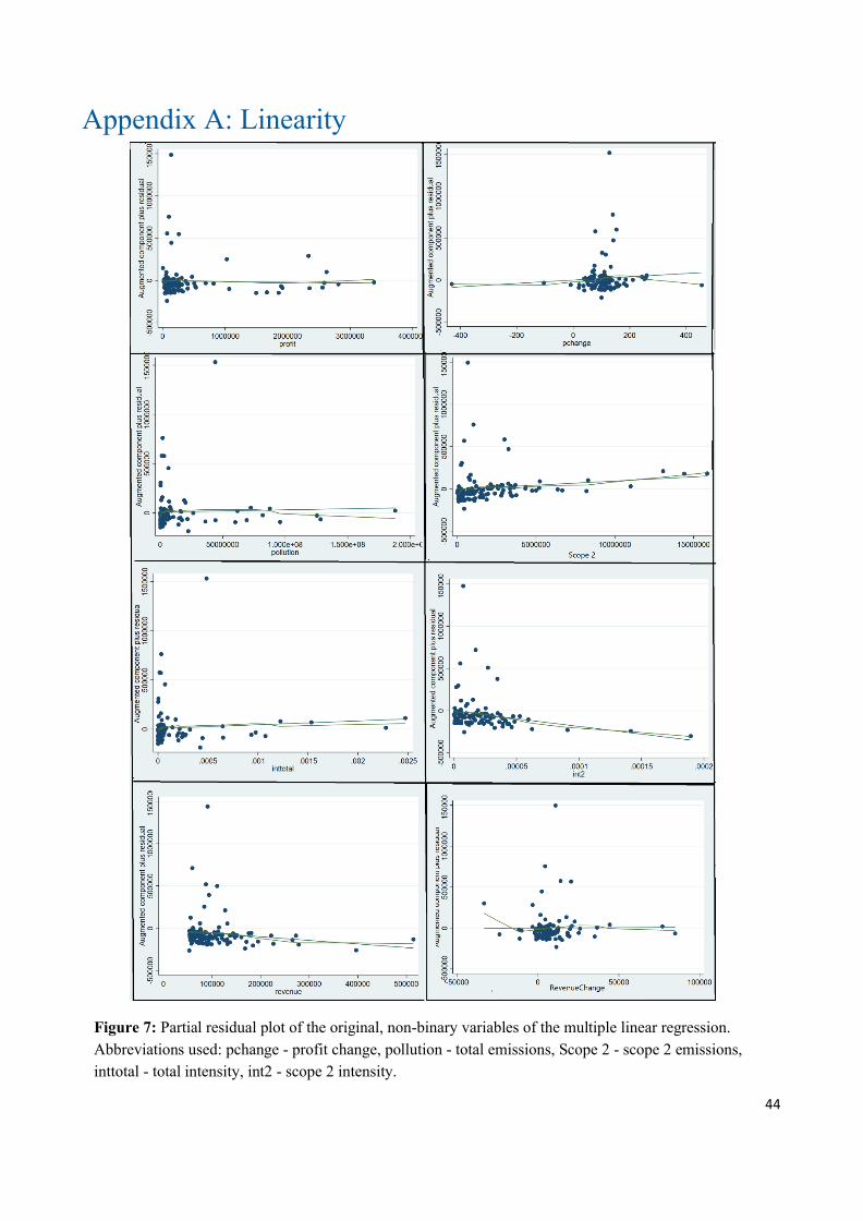
44

Appendix A: Linearity

Figure 7: Partial residual plot of the original, non-binary variables of the multiple linear regression.Abbreviations used: pchange - profit change, pollution - total emissions, Scope 2 - scope 2 emissions,inttotal - total intensity, int2 - scope 2 intensity.

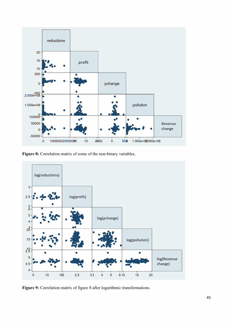
45

Figure 8: Correlation matrix of some of the non-binary variables.

Figure 9: Correlation matrix of figure 8 after logarithmic transformations.

46

Appendix B: Normality of residuals

Figure 10: On the left is a plot representing the residuals after logarithmic transformation and on the right aplot of the residuals before the transformation.

Appendix C: Lack of multicollinearity

Table 7: The correlation matrix of all variables is shown. The non-binary variables are transformed intologarithms.

log(revenue) log(pollution) log(Scope2) log(inttotal) log(int2) oil retail transport IT------------ -+ --------- --------- --------- --------- --------- --------- --------- --------- ---------

log(revenue) | 1log(pollution) | -0.0399 1log(Scope2) | 0.2677 0.6301 1log(inttotal) | -0.2444 0.9787 0.5564 1

log(int2) | -0.2818 0.6659 0.9543 0.653 1oil | -0.2299 0.6299 -0.0822 0.6585 0.6913 1

retail | -0.054 0.0783 0.2648 0.0871 0.0213 -0.1242 1transport | 0.449 0.1146 0.2622 0.0189 0.0926 -0.1826 -0.1089 1

IT | 0.1623 0.0343 0.3688 -0.0001 -0.2654 -0.1826 -0.1089 -0.16 1electronics | -0.1704 -0.0405 0.1491 -0.0042 0.0143 -0.1826 -0.1089 -0.16 -0.16

finance | -0.045 -0.6954 -0.6022 -0.6656 -0.6084 -0.2331 -0.139 -0.2043 -0.2043europe | -0.015 -0.0216 -0.2958 -0.0179 0.0706 0.1726 0.0476 0.07 -0.133

us | 0.1484 -0.132 0.0312 -0.1586 -0.2117 -0.1687 -0.2128 -0.3127 0.3056compliance | -0.2504 0.4611 0.1164 0.4989 0.4866 0.4629 0.0077 0.0113 -0.0708

log(Revenuechange) | 0.2523 0.4584 0.2887 0.393 0.3584 0.2494 -0.1038 0.3445 0.1258log(profit) | 0.3264 -0.3491 -0.109 -0.4059 -0.4791 -0.2021 -0.0789 0.012 0.0884

log(pchange) | 0.2476 -0.2193 -0.3284 -0.2638 -0.221 -0.0134 0.0316 -0.1683 -0.205| electronics finance europe us compliance log(Revenuechange) log(profit) log(pchange)

------------ -+ ------------ --------- --------- --------- --------- --------- --------- ---------electronics | 1

finance | -0.2043 1europe | -0.3361 0.2622 1

us | 0.0995 -0.0484 -0.6568 1compliance | 0.0113 -0.3352 0.0813 -0.0946 1

log(Revenuechange) | -0.1245 -0.4363 -0.2396 0.1118 0.3039 1log(profit) | -0.2979 0.6813 0.2334 0.0478 -0.2543 -0.2396 1

log(pchange) | 0.0098 0.0229 -0.0412 0.2774 -0.0949 0.1331 -0.0196 1