demographic and housing demand analysis.passaic county.new jersey

DEMOGRAPHICS, POPULATION AND HOUSING DEMANDS

Passaic County, New Jersey

FALL 2016 Methods of

Planning

Analysis II

Himadri Kundu M.C.R.P. 2017EJB School ofPlanning andPublic PolicyRutgersUniversity

image source: www.google.com

Himadri Kundu

1

Introduction

In order to completely understand what should be the visions for future growth for any community, understanding

both its temporal and spatial population distribution is essential. Only then the future development decisions can

be the most effective to serve the needs of the community.

The primary objective of this paper is the

exploration of the various ways to project

future populations, analyze and compare

the effectiveness of those predictions to

explain the current and future conditions.

Passaic County in New Jersey was chosen as

the study area due to its diversity and ability

to represent the northeastern metropolitan

region of United States of America.

Location

Passaic County, located in the northeastern

part of New Jersey contains a diverse

landscape from both geographic and

demographic aspects. Being 8 miles away

from Manhattan at one point, the

southeastern part of the County is

expectedly urbanized. However, a number

of municipalities like Bloomingdale,

Pompton Lakes, Ringwood, Wanaque, and

West Milford located in the northwestern

part of Passaic County are included in the protected region of New Jersey’s highland preservation area which are

relatively underdeveloped and extends to the foothills of the Appalachian Mountains. The diversity in spatial

distribution of urban development in the Passaic County can mostly be attributable to its geographical location

around the Tri-state area, shape, and transportation infrastructure. Close to two-thirds of the County’s total

population is concentrated in its southern part with urban centers like Paterson, and Clifton, and suburban

township of Wayne due to the proximity as well as the transportation access to the regional employment centers,

such as New York City. The spatial distribution of these communities within the Passaic County as well that of the

county within New Jersey can be seen in Figure 1(A).

Figure 1(A): Location of Passaic County, New Jersey

Himadri Kundu

2

The presence of transportation infrastructure in the county as shown in Figure 2 also follows these population

centers, with Garden State Parkway and US

Interstate passing through Paterson, and NJ

Transit’s Main Line connecting both Clifton

and Paterson to New York City. The “skinny

part” of Passaic County marks the northern

extent of major transportation

infrastructures with US Interstate 287 near

to Pompton Lakes. However, the two

airports that the county has are located in

the northwestern parts and the ones closer

to the major urban centers are in the

neighboring counties.

Background and Demographics

Rich in both pre and post-independence

history, Patterson City in Passaic County was

the first planned industrial city of the US

(“Paterson: History”, City-Data.com, 2016)

which is shown in the early map of 1872 in

Figure 1(B), and by the start of the 20th

century its population had grown to become the fifteenth largest of the country. Being an industrial hub, different

types of industries, most of them manufacturing clustered around the Great Falls in Paterson and other location

along the Passaic River. The prime industrial location attracted a continuous stream of immigrant workers

throughout the nineteenth and the early part of the twentieth century. However, during the early part of the

twentieth century Paterson saw a few problems with labor strikes, and then the Great Depression was followed

by wide-spread de-industrialization with the silk industry dying away. Even though it tried to bounce back like

before the slow death of its other manufacturing industries moving away over the years to newer and cheaper

towns in other counties, Passaic County suffered a large loss in population and along with that its importance as

an industrial center diminished. This period saw a slowdown in the inward migration with eventual emigration

from the major urban centers like Paterson and (the City of) Passaic.

Figure 2: Transportation access for Passaic County, New Jersey

Himadri Kundu

3

Post World War II however the trend reversed after 1950s when the suburban communities of Passaic County led

by Wayne Township saw rapid growth in population as middle class residents flowed in not only from the local

cities but also from regional centers like New York City. There are still a few remnants of the garment industry in

Paterson, but it mostly serves as a historic importance with landmark buildings, or industrial buildings converted

to newer uses. However, currently the city is in transition into a service provider for the surrounding municipalities

in the East Coast; mostly focusing on financial, sales and healthcare industries for its new economic growth.

The increasing trend of Passaic County’s population can be seen from Table 1, when it grew by 151,429 between

the years of 1940 to 1970 (US Census Bureau). Post war Passaic County has experienced a decrease in population

only once, that too slightly which was from 1970 to 1980, as shown by Figure 3. However, the growing trend of

population still continues till today, even though the percentage increase in population for the county has slowed

down from an 8% increase in 2000 to a mere 2% increase in 2010, but an imminent drop in the total population

does not seem to be on the cards in the near future due to transition of its largest city Paterson into a service

provider for the surrounding municipalities and well connected suburban communities. Also, the economic

slowdown of 2008 might have been influential in the slight slowdown of the population growth rate.

Figure 1(B): Passaic County, New Jersey in 1872

Source: “Historical Maps of New Jersey”, url: http://mapmaker.rutgers.edu/1872Atlas/Bergen_Passaic_1872.jpg

Himadri Kundu

4

Today the median household income of Passaic County is $59,513 (2010-2014, American Community Survey 5-

Year Estimate, 2014), which is above the national median but still well below its wealthy neighbors of Morris

County, Bergen County or Sussex County. According to the 2010 US Census, Passaic County was the ninth most

populous county in the state with a total work force population of 386,557 in 2010, accounting for 64.6 % of the

total population. As on 2010, the majority of the population is White constituting 62.65% of the total population,

while only 12.8% were reported to be African American and 37% were reported to be Hispanic or Latino of any

race. The percentage of females in 2010 was 51.5% slightly higher than that of the State’s ratio. The following

section analyzes the historic population characteristics and trends in Passaic County, in particular age and sex.

Population by Age and Sex

Age-sex pyramids were prepared in order to examine the historic and current population demographics of Passaic

County with respect to age and sex in a more detailed manner. This section aims at tracing the recent trends in

population cohorts by using the Decennial data collected from US Census

1990 Population

In 1990, as shown in Figure 4, there is a

considerable bulge in the middle of the age-

sex pyramid, mostly for the age cohorts of

25 - 29 and 30 - 34 years, for both genders.

This clearly indicates the effects of the

suburbanization by the middle class

families that begun during the 1950s, which

were mostly young families and the age

cohorts of 30 – 34 and 25 – 29 are most

likely comprise of their children. The “baby

boom” during the post war period was

common across the country, in particular in

the growing suburban communities. The

major bulk of the population appears to be

concentrated in the middle portion

between the age cohorts of 40 – 44 and 15

– 19, before it tapers off on either side with the exception of the youngest age cohort of 0 – 4. These young cohorts

are the pre- “millennials” and to a certain extent the “baby boomers” are also responsible for the high numbers

30,000 20,000 10,000 0 10,000 20,000 30,000

0-4

5-9

10-14

15-19

20-24

25-29

30-34

35-39

40-44

45-49

50-54

55-59

60-64

65-69

70-74

75-79

80-84

85+

Population (persons)

Age

Co

ho

rt (

in y

ears

)

Figure 4: 1990 Population, Passsaic County, New Jersey

Females

Males

Source: 1990 US Census

Himadri Kundu

5

in this age cohort as well, since by this decade few of them also started having families of their own. The interesting

thing to note in this year’s population is that the number of males relative to females in each age cohort starts to

decrease drastically only when we move above the age cohort of 45 – 49, which is reflective of the lower survival

rates for males in general above middle ages.

2000 Population

In 2000, as shown by Figure 5, the

“baby boomers” have grown up to

the age cohorts of 40 – 44 down till

30 – 34, which is where the majority

of the bulge in the age-sex pyramid

appears to be. However, there is

hardly any difference to the previous

decade’s population distribution

across ages other than the heavy

bottom of the pyramid, which clearly

marks the birth of the “millennials” in

the age cohorts of 5 – 9 and 0 – 4.

Since by this time most of the “baby

boomers” have grown up to be adults

and were likely to have their own

children, the age cohorts of the

“millennials” are pretty close in

numbers to that of their parents. The

parents of the “baby boomers”

however shows a decrease in their

numbers as they grew older with decreasing survival rates and also some may have migrated to warmer climates.

Thus the tapering of the pyramid is greater for this year.

30,000 20,000 10,000 0 10,000 20,000 30,000

0-4

5-9

10-14

15-19

20-24

25-29

30-34

35-39

40-44

45-49

50-54

55-59

60-64

65-69

70-74

75-79

80-84

85+


Age

Co

ho

rt (

in y

ears

)


Females in2000

Males in2000


Himadri Kundu

6

2010 Population

The population in 2010, as shown in Figure 6, with a bulge between the upper middle age cohorts of 40 – 44 and

50 – 54 that represent the “baby boomers”. Although their numbers have decreased slightly from those in 2000,

as few would be likely to move to warmer climates leaving their large suburban housing once their children moved

out with their own families. This trend of a slight decrease is also visible from Figure 7 when we compare the other

age cohorts of 25 – 29 and 30 - 34 in

2000 population with that of their

corresponding older cohorts in 2010

population pyramid. In the 2010

population, one of the “millennials”

age cohort of 15 – 19 has the highest

numbers, closely followed by their

counterparts and the adjacent age

cohorts of the pre – “millennials” to

create a firm younger foundation of

the pyramid. The numbers in the

youngest age cohorts of 0 – 4 and also

that of 5 – 9 saw only a slight decrease

from that of 2000, which evidently

points to the strong middle age

groups starting new families and also

the late “baby boomers” who are still

within the fertility range.

Overall, the recent trend in the

population have been dominated by both the “baby boomers” and the “millennials” that improved, and create a

strong and robust age-sex pyramid of 2010. This suggest a stable and fertile period for population growth of the

county as it shifts from an industrial center into a more residential and service sector population. The increase in

the population of the oldest cohort in 2010 (Figure7) also shows the improvement in health care facilities as well

as the quality of life. Thus improving the survival rates of this cohort.

30,000 20,000 10,000 0 10,000 20,000 30,000

0-4

5-9

10-14

15-19

20-24

25-29

30-34

35-39

40-44

45-49

50-54

55-59

60-64

65-69

70-74

75-79

80-84

85+


Age

Co

ho

rt (

in y

ears

)


Femalesin 2010

Males in2010


Himadri Kundu

7

Population Projections

Trend Extrapolation

The total population counts for the years 1940 to 2000 were collected for Passaic County from the US Census.

Population projections for 2010 were created using seven different methods of direct aggregate models for

population extrapolation from this data. Every model has its own strengths and weaknesses, but the model with

the “best” performance was determined statistically by evaluating their R2 values, Mean Absolute Percentage

Errors (MAPE) and comparing the predicted values with the actual data of 2010 population from the US Census.

The value of R2 indicates how much of the variability in the population trend can be explained by the model. For

example, say the R2 value for a particular model is 0.8, that means the model can only explain 80% of the variability

of the population trend data. MAPE value also displays the average accuracy of the model through mean

percentage error. So, higher value of R2 shows better fit, while a lower value of MAPE is better. The summary of

the results from each of the seven models can be seen from Table 1 below. It should be noted that the Moving

Average method uses averaging historic values to predict the future values and since there is no equation for this

method, it does not have a R2 value. If we were to evaluate the models purely based on the values of R2, then

30,000 20,000 10,000 0 10,000 20,000 30,000

0-4

5-9

10-14

15-19

20-24

25-29

30-34

35-39

40-44

45-49

50-54

55-59

60-64

65-69

70-74

75-79

80-84

85+


Age

Co

ho

rt (

in y

ears

)

Figure 7: Comparison of 2000 & 2010 Population, Passsaic County, New Jersey

Females in2000

Males in2000

Males in2010

Females in2010

Source: 2000 and 2010 US Census

Himadri Kundu

8

probably we would end up choosing one that fits the data the best, which in this case would be the red trend-line

in Figure 8 over the black one in the same graph. The red trend-line is of a Polynomial model in the fifth order,

however, it was not included in the comparison and instead the polynomial model of the second order (blue line)

was chosen over it. The reason behind this was the uneven nature of prediction, even in the short range which

results in overshooting the predicted value for 2010 population by almost 80,000 even though the R2 value was

almost perfect at 0.9953 that explains 99.53% of the population trend between 1940 and 2000. But this where

the absolute percentage error for 2010 (2010 APE) comes into play. The 2010 APE shows how accurate is the

prediction for 2010, and this is where most of the models did poorly even if they had high R2 values other than

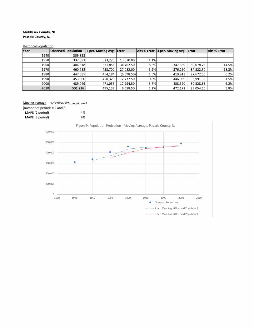
the Power and the Moving Average (2 period) models. The reason behind choosing the moving average model for

2 periods over a 3 period moving average is almost similar, as the former fared better in explaining the population

trend and also in predicting the 2010 population with a lower 2010 APE which can be seen from both Table 1 and

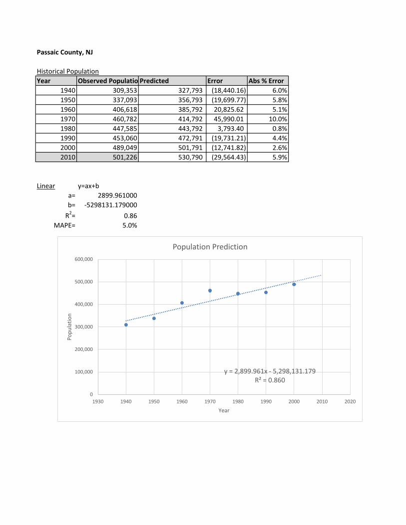
also the red graph in Figure 9. As for the linear and the logarithmic models both ended up having a similar

prediction with a 2010 APE value of around 5.8% and similar R2 values of 0.86, and in both instances overshooting

the population by similar amounts. As a result, the MAPEs for these models were also in the higher range as can

be seen from the color coded values in Table 1. The exponential model overshot the observed population in its

prediction by the highest margin of around 48,775. When we compare the various R2 values between different

models, even though the polynomial model of the second order comes close to the highest value of 0.941 of the

power model, still its 2010 APE and the MAPE values are much higher than the power model’s.

Table 1: Comparing parameter estimates for 2010 population prediction by trend extrapolation

Model Equation R2 MAPE Actual 2010

Predicted 2010 2010 APE

Linear y=ax+b 0.860 5.1% 501,226 530,790 5.9%

Exponential y=a*ebx 0.842 6.1% 501,226 550,002 9.7%

Logarithmic y=a+b*ln(x) 0.862 5.0% 501,226 530,062 5.8%

Polynomial y=ax2+bx+c 0.934 3.7% 501,226 472,552 5.7%

Power y=a*xb 0.941 2.9% 501,226 504,280 0.6%

Moving average (2 periods) yt=avg(yt-1,yt-2) N.A. 4.0% 501,226

495,138 1.2%

Moving average (3 periods) yt=avg(yt-1,yt-2,yt-3) N.A. 9.0% 501,226

472,172 5.8%

Modified exponential y=c-a*(b^x) 0.874 4.3% 501,226 516,535 3.1%


Himadri Kundu

9

Hence after the comparison between the Models in Table 1 in order to choose the best model for our objective,

Power and 2 period Moving Average models which have the lowest 2010 APE and MAPE with the Power Model

having a high R2 value as well. The 2010 APE in case of the Power Model is almost half of that of the Moving

Average model, and also has a high R2 value of 0.941 with a MAPE of 2.9%. Further, the moving average model

will always underestimate for a growing population trend as it averages the previous lower population to derive

its estimate of the future. From these facts it is obvious that the prediction from the Power curve comes closest

to the actual 2010 population even though it overshoots by 3053.

The Modified Exponential Model (Figure 10) utilizes the logarithmic transformation of an exponential equation to

fit a linear curve on the data with the consideration for a maximum ceiling population of the county which is the

capacity that can be supported by the resources of the county over the long term. This ‘capacity’ parameter (c)

was assumed on the basis that even though there may be ample amount of space available in Passaic County,

however most of the rural northwest comes under preservation areas and also suburban communities are mostly

built up already thus there is hardly enough room for a rapid growth of the population in the near future from

“greenfield” development. However, there may be room for increased density with vertical construction,

redevelopment or infill, and revitalization of some of the decaying old neighborhoods and those of the built up

southern urban parts of the county, but these types of developmental growth are hardly rapid enough to be

considered for a short term projection. It should be noted that, there is enough room for growth from the future

long term perspective though. On the basis of these consideration about the spatial characteristics of Passaic

County, the capacity for the County was fixed at 800,000 which makes the modified exponential model somewhat

y = -49.25321x2 + 196,957.62500x - 196,425,229.21429R² = 0.93409

y = -0.0033x5 + 32.7442x4 - 129,728.5171x3 + 256,967,412.7530x2 - 254,484,947,838.0310x + 100,803,961,008,307.0000

R² = 0.9953

0

100,000

200,000

300,000

400,000

500,000

600,000

700,000

1930 1940 1950 1960 1970 1980 1990 2000 2010 2020

Po

pu

lati

on

(p

erso

ns)

Years

Figure 8: Population Projection - Polynomial Model, Passaic County, NJ

Observed Population

Poly. (Observed Population)

Poly. (Observed Population)

Power (Observed Population) Source: US Decennial Census

Himadri Kundu

10

intuitive of the geographic realities. Still the prediction values for 2010 overshoots by 15,309 with an APE of 3.1%,

MAPE of 4.3% and R2 of 0.874. Thus, even though the modified exponential model can account for long term

growth characteristics in a better way and thus may be better for long term population projection, for the

prediction of 2010 population based on the historic population trend from 1940 to 2000, the Power model with

its geometric function was the “best” model in this scenario.

0

100000

200000

300000

400000

500000

600000

1930 1940 1950 1960 1970 1980 1990 2000 2010 2020

Po

pu

lati

on

Years

Figure 10: Population Projection - Modified Exponential Model, Passaic County, NJ

Estimated Population

Observed Population

Source: US Decennial Census

0

100,000

200,000

300,000

400,000

500,000

600,000

1930 1940 1950 1960 1970 1980 1990 2000 2010

Po

pu

lati

on

Figure 9: Population Projection - Moving Average Model, Passaic County, NJ

Observed Population

2 per. Mov. Avg. (ObservedPopulation)3 per. Mov. Avg. (ObservedPopulation)


Himadri Kundu

11

Cohort Component Model

There is another way to predict future population other than the historic trend extrapolation by direct aggregate

models. In this approach, which is a part of the direct component models, we would be using one of its bottom-

up approaches for projection of future population using the Cohort Component Model.

The cohort component model takes into account various population growth parameters or sources; such as

number of births, deaths as well as migration. Thus various county-wide data for the years of 1990 and 2000 had

to be collected to project the 2010 population using this model which included the following: number of bkirths

per child-bearing cohorts, number of deaths per cohorts and total population per cohort for both the years

mentioned above. Several rates were required based on these data like fertility rates, survival rates and birth rates

to accurately estimate the 2010 population from the aspect of births and deaths reported for the county. It is

important to note here that fertility rates county-wide were not available for both the years and the 2000 data

had to be used in both cases. Also, State-wide data for birth rates as percentage of males and females instead of

county specific ones due to unavailability. Further, as the model factors in migration for determining the

population growth, residual migration method was used by adding the difference between the projected the

observed population of 2000 to the projected population of 2010. Thus the projection of the 2010 population

from the actual 2000 population without residual migration was 529,022 and that with the residual migration was

500,434 assuming the migrating population stays the same for 2010 with that of 2000. On comparison to the

actual 2010 population the projected population from this method underestimates by a mere count of 792, which

shows the power of this bottom up approach, even when there were lot of assumptions and data not available

for the intermediary steps.

30,000 20,000 10,000 0 10,000 20,000 30,000

0-4

5-9

10-14

15-19

20-24

25-29

30-34

35-39

40-44

45-49

50-54

55-59

60-64

65-69

70-74

75-79

80-84

85+


Age

Co

ho

rt (

in y

ears

)

Figure 11: Estimated Population in 2010 of Passaic County, NJ

Estimated Males Estimated Females


30,000 20,000 10,000 0 10,000 20,000 30,000

0-45-9

10-1415-1920-2425-2930-3435-3940-4445-4950-5455-5960-6465-6970-7475-7980-84

85+


Age

Co

ho

rt (

in y

ears

)

Figure 12: Observed Population in 2010 of Passaic County, NJ

Observed Males Observed Female


Himadri Kundu

12

The unique ability of this model is also its power to analyze the projected population by age cohorts and again by

sex in each cohort. Thus on the basis of the results from this model age-sex pyramid was constructed for the which

is visible in Figure 11. A comparative pyramid in Figure 13 shows how similar the projected cohorts to the actual

2010 data. Other than a few major differences in the extreme ends, there are only minor differences in the middles

age cohorts, and the shape of both the pyramids are almost similar. The differences in the youngest age cohorts

may steam from the fact that the data for birth rates used to project the intermediary populations of 1995 and

that of 2000 were not that of 1990 due to unavailability and instead that of 2000 had to be used. Further, the

difference between the projected and actual age cohorts above 70 – 79 increases drastically relative to the rest

and also it is more pronounced for the males than the females of 85+ age cohorts. One of the reasons for this

difference can be the use of annual crude mortality rates to derive the survival rates over a period of five years,

and thus increasing the number to a greater extent than in reality, which then increases the residual migration

counts and ultimately reduces the projected population of the age cohorts in the 2010 population. The use of the

2000 fertility rates for estimating the intermediary populations of 1995, 2000 and 2005 also leads to an

overestimation of total number of births, which then leads to higher residual migration numbers and ultimately a

lower projection for the for the 0 – 4 age cohorts of 2010. Another reason that might have contributed would be

from to the measurement error of the

fertility rates itself, since the total

population that was used to calculate

the fertility rates (Natality Rates) and the

number of births for the county in 2003

– 2006 by Center for Disease Control was

almost seventy-five percent that of the

actual population for both 1990 and

2000 respectively. Further, since the

fertility rates for ages under 15 years

and over 44 years were not available

even though few births were recorded

for these groups, so the fertility rates for

the adjacent groups were used as

estimates for them. This could also

increase the number of total births for

the intermediary populations to cause

the differences in the youngest age

cohorts.

The population projections using direct

component methods like the cohort

component model are extremely critical

from the aspect of future community planning. These estimated future cohort populations will help define the

predict the future demand for services in the community. In particular, the importance of housing demand for

planning is crucial.

25,000 20,000 15,000 10,000 5,000 0 5,000 10,000 15,000 20,000 25,000

0-4

5-9

10-14

15-19

20-24

25-29

30-34

35-39

40-44

45-49

50-54

55-59

60-64

65-69

70-74

75-79

80-84

85+


Age

Co

ho

rt (

in y

ears

)

Figure 13: Comparison between Estimated and Observed Population in 2010 of Passaic County, NJ

Observed Female Observed Males


Himadri Kundu

13

Housing Demands The demand for unmet housing in Passaic County were calculated based on the data from US Census for 2000 and

2010, which reveals that out of the 175,966 units only 5.2% or 9,181 units were vacant in 2010. However, the

vacancy rate in 2000 was only 3.6%. Even though the total populations and predicted future populations are a

major factor in estimating whether or not the supply of the housing stock will be able to meet the demands in the

future, however, total population is not the only consideration. There are other critical parameters for the

estimation of housing

demands such as; housing

population and size, total

housing units, number of

households, occupied units,

housing units that needs to be

replaced, the building permits

issued, and those that are

completed. Thus using all these

data collected from both the

2000 and 2010 Census, the

unmet housing demand was

estimated for the period of 2010 – 2020.

The projection for 2020 population was done using a simple linear model that estimates the total population of

Passaic County in 2020 to be 513,403, which is a 2% increase from the observed population in 2010. Similarly,

assuming a linear growth rate for the number of households in Passaic County for this period the estimated

households for 2020 was found to be 169,372. Now, if it is assumed that the housing stock remains unchanged in

2020 from what it was observed in 2010, the vacancy rate comes down to 3.5%, which might not look terribly bad

considering the fact that it is the same as that of 2000. However, during the 1990 – 2000 decade, the growth rate

for total population was 8%, which is four times higher than what has been predicted for the coming decade in

this projection. One of the reason for this low vacancy rates and high population growth rate the prices in the

housing market shot up not only in the county but state-wide, which ultimately had some role to play in the

housing bubble of 2008. In order to avoid such economic and also social ramifications for Passaic County there

needs to be informed decision making from the policy makers to improve the supply and quality of housing.

Housing demand that is currently not met as per the projections based on certain assumption and the Census data

was calculated from the difference between the total number of units needed from 2000 – 2020 and the total

Table 2: Housing Demand Estimation for 2020 in Passaic County, New Jersey

Housing Demand

Change in the Number of of Households 2000-2020 5,306

Change in the Number of Vacant Units 2000-2020 5,978

Units Lost to Disaster 2000-2020 3,401

Units Lost to Conversion 2000-2020 850

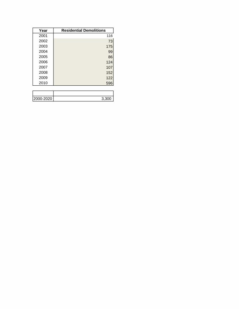
Units Lost to Demolition 2000-2020 3,300

Units that Must Be Replaced 2000-2020 7,551

Total Number of Units Needed 2000-2020 18,835

Projected Housing Completions 2001-2020 8,613

Unmet Housing Demand 2011-2020 10,222

Himadri Kundu

14

number of housing completions during that period. The number of housing completions was calculated from the

count-wide permits information, with the consideration of that the rate of completions will stay the same over

the period of 2010 – 2020 to that of the previous decade. While the total number of units required was calculated

from the change in housing units being occupied, number of households, change in vacant units and also the

number of units that need to be replaced. The requirement for replacement could steam from several factors like

the loss to disasters, or conversions and demolitions. The number of units lost to demolition was available from

the state department, but those lost to disasters and conversion was determined at rate on the basis of local

knowledge of the county. It is interesting to note that the during 2010 the number of housing units lost to

demolition was the highest in the last decade while 2009 saw the second fewest building permits for residential

constructions issued. May be one of the reasons for such an abnormality in the trend could be attributable to the

crash of the housing market in 2008, which slowed down the supply considerably. This data does not include the

units lost to the consecutive hurricanes Irene and Sandy in 2011 and 2012, which will severely impact the housing

market in Passaic County due to its considerable effect on many of the suburban and urban communities

throughout the county, in particular along the Passaic River. Thus the rate to calculate the units lost to disaster

was estimated at 2% of the housing stock, however the actual number may be even larger. Loss to conversion

was estimated at a moderate rate of 0.5% of the housing stock. Thus, through the above mentioned process the

unmet housing demand was estimated at 10,222 units for the period of 2000 – 2020. This signifies that the county

is in need of 10,222 units till 2020 to meet the demand expected from the linear growth of the projected

population.

The projected housing demand is expected to exceed the housing supply by 2020 on the basis of the linear

population and household growth model used here. Like it has been mentioned above this could have extreme

consequences on the communities if new housing opportunities both in the urban and the suburban areas are not

developed. One of the outcomes if the unmet demands are not catered for, will be the increase in the prices and

rents for housing, which in turn might force many to look for housing elsewhere and even outside of the county.

The loss of tax revenues for the community even if a fraction of the population in proportion of the unmet housing

demand or some part of it moves out of the county. Further, the rate of growth for average household size has

not been extremely high but still it is growing from 2.92 in 2000 to 2.96 in 2020, which might indicate the demand

for single family housing units will be on the rise. May be this is one of the reason for the lower number of

completion permits for multifamily units, relative to the single family ones. However, based on the trends of the

“millennials” wanting to move back into the cities or urban centers, this factor can outweigh the assumption on

the average household sizes. Further, the types of units lost to different factors needs to be analyzed with context

of where and which type of housing demands are not being met. The spatial context of the demand in relation to

Himadri Kundu

15

the demographic preferences based on lifestyle changes will be a key factor in determining how the unmet

housing demand influence the population and life in this county.

Conclusion

This paper’s effort at the prediction of the population based on the historical trends as well as cohort component

models with its application on the housing market, can be influential in taking decisions for future policy making.

In reality there are a number of factors that can influence the demographics of any place and without analyzing

the specifics, accurate predictions are not possible but only at the cost of huge efforts. However, most of the

models used here came extremely close to the actual population of 2010, with the power model being 0.6% and

the cohort component model being even closer at 0.16% of the actual population of 2010. The slight variations

shown by the other models might be due to the volatile economic conditions during the late 2000s, when families

might have decided against migration, or to hold of starting a family. The slowdown in the housing supply was

evident from the permits issued and the demolition of units we have already seen.

The importance of this type of study when projecting for the future needs of an y community are significant. Since

such analysis, are required as a pre-requisite for informed decision making to improve the planning and public

policy formulation which can impact the community in the longer run. As it has been mentioned earlier, estimating

and predicting the future population is the heart of understanding how any community can prosper in the future.

Passaic County had been able to maintain a steady and almost stable growth rate despite its struggle with the

historical industrial center. Even though the growth rate had been modest, it has lead the population to have a

robust structure with respect different age cohorts and create a more diverse community, rather than being

overwhelmed by the suburban sprawl of the 1950s and 60s. Its major urban centers like that of Paterson and

Passaic City can promote urban redevelopment to support the younger generations of the millennials and post

millennials who generally have been seen to prefer an urban setting but need modest rents. Thus by improving

the housing supply at the urban center with increase in density, a more vibrant core could be developed which

has the high likelihood of increasing the demand and revenue through the transit access to New York City and

other regional employment centers.

Himadri Kundu

16

References “Paterson: History”, City-Data.com. Retrieved November 2016. url: http://www.city-data.com/#data

“Historical Maps of New Jersey”. Retrieved November 2016. url:

http://mapmaker.rutgers.edu/1872Atlas/Bergen_Passaic_1872.jpg

US Census Bureau. “State & County QuickFacts: Passaic County, New Jersey”. Retrieved November 2016. url:

http://www.census.gov/quickfacts/table/PST045215/34031,00

http://www.city-data.com/#data

http://mapmaker.rutgers.edu/1872Atlas/Bergen_Passaic_1872.jpg

http://www.census.gov/quickfacts/table/PST045215/34031,00

Appendix

Passaic County, NJ

1990 Age/SexAge Total Females Male Males0-4 36,037 17759 18,278 -18,2785-9 30,620 14835 15,785 -15,78510-14 30,160 14758 15,402 -15,40215-19 33,477 16560 16,917 -16,91720-24 38,567 19135 19,432 -19,43225-29 42,035 20957 21,078 -21,07830-34 41,559 20846 20,713 -20,71335-39 36,281 18337 17,944 -17,94440-44 33,289 17134 16,155 -16,15545-49 26,923 14036 12,887 -12,88750-54 22,155 11561 10,594 -10,59455-59 20,518 10733 9,785 -9,78560-64 20,596 11009 9,587 -9,58765-69 18,893 10558 8,335 -8,33570-74 14,871 8774 6,097 -6,09775-79 11,674 7305 4,369 -4,36980-84 7,389 4851 2,538 -2,53885+ 5,832 4,329 1,503 -1,503

470,876

2000 Age/SexAge Total Females in 20Male Males in 20000-4 36,129 17764 18365 -183655-9 37,178 18386 18792 -1879210-14 34,776 16997 17779 -1777915-19 32,341 15716 16625 -1662520-24 32,540 16208 16332 -1633225-29 34,818 17435 17383 -1738330-34 38,678 19343 19335 -1933535-39 40,932 20537 20395 -2039540-44 38,591 19637 18954 -1895445-49 32,827 16709 16118 -1611850-54 29,765 15533 14232 -1423255-59 23,207 12306 10901 -1090160-64 18,234 9672 8562 -856265-69 15,520 8594 6926 -692670-74 14,573 8431 6142 -614275-79 12,626 7650 4976 -497680-84 8,617 5595 3022 -302285+ 7,697 5528 2169 -2169

489,049

30,000 20,000 10,000 0 10,000 20,000 30,000

0-4

5-9

10-14

15-19

20-24

25-29

30-34

35-39

40-44

45-49

50-54

55-59

60-64

65-69

70-74

75-79

80-84

85+


Age

Coho

rt (i

n ye

ars)


Females

Males

30,000 20,000 10,000 0 10,000 20,000 30,000

0-4

5-9

10-14

15-19

20-24

25-29

30-34

35-39

40-44

45-49

50-54

55-59

60-64

65-69

70-74

75-79

80-84

85+

Population

Age

Coho

rt (i

n ye

ars)


Femalesin 2000

Males in2000

2010 Age/SexAge Total Females in 20Male Males in 20100-4 34247 16669 17578 -175785-9 34008 16704 17304 -1730410-14 34536 16852 17684 -1768415-19 37604 18555 19049 -1904920-24 36025 17872 18153 -1815325-29 33501 16890 16611 -1661130-34 33173 16919 16254 -1625435-39 33499 17201 16298 -1629840-44 35615 18142 17473 -1747345-49 37411 19114 18297 -1829750-54 35704 18540 17164 -1716455-59 30182 15646 14536 -1453660-64 25397 13527 11870 -1187065-69 18226 9926 8300 -830070-74 13624 7569 6055 -605575-79 10679 6339 4340 -434080-84 8784 5385 3399 -339985+ 9011 6252 2759 -2759

501,22630,000 20,000 10,000 0 10,000 20,000 30,000

0-4

5-9

10-14

15-19

20-24

25-29

30-34

35-39

40-44

45-49

50-54

55-59

60-64

65-69

70-74

75-79

80-84

85+

Population

Age

Coho

rt (i

n ye

ars)

Figure 7: Comparison of 2000 & 2010 Population, Passsaic County, New Jersey

Females in2000Malesin 2000

Malesin 2010

Females in2010

25,000 20,000 15,000 10,000 5,000 0 5,000 10,000 15,000 20,000 25,000

0-4

5-9

10-14

15-19

20-24

25-29

30-34

35-39

40-44

45-49

50-54

55-59

60-64

65-69

70-74

75-79

80-84

85+

Population

Age

Coho

rt (i

n ye

ars)


Femalesin 2010

Males in2010

Passaic County, NJ

Historical PopulationYear Observed Populatio Predicted Error Abs % Error

1940 309,353 327,793 (18,440.16) 6.0%1950 337,093 356,793 (19,699.77) 5.8%1960 406,618 385,792 20,825.62 5.1%1970 460,782 414,792 45,990.01 10.0%1980 447,585 443,792 3,793.40 0.8%1990 453,060 472,791 (19,731.21) 4.4%2000 489,049 501,791 (12,741.82) 2.6%2010 501,226 530,790 (29,564.43) 5.9%

Linear y=ax+ba= 2899.961000b= -5298131.179000

R2= 0.86MAPE= 5.0%

y = 2,899.961x - 5,298,131.179R² = 0.860

0

100,000

200,000

300,000

400,000

500,000

600,000

1930 1940 1950 1960 1970 1980 1990 2000 2010 2020

Popu

latio

n

Year

Population Prediction

309,353337,093

406,618460,782 447,585 453,060

489,049 501,226

0

100,000

200,000

300,000

400,000

500,000

600,000

1930 1940 1950 1960 1970 1980 1990 2000 2010 2020

Popu

latio

n (p

erso

ns)

Years

Observed Population

Passaic County, NJ

Historical PopulationYear X Observed Population Predicted Error Abs % Error

1940 1 309,353 328,515 (19,161.75) 6.2%1950 2 337,093 353,613 (16,519.52) 4.9%1960 3 406,618 380,628 25,990.30 6.4%1970 4 460,782 409,707 51,075.22 11.1%1980 5 447,585 441,007 6,577.57 1.5%1990 6 453,060 474,699 (21,639.38) 4.8%2000 7 489,049 510,965 (21,916.32) 4.5%2010 8 501,226 550,002 (48,775.90) 9.7%

Exponential y=a*ebx

a= 305198b= 0.0736

R2= 0.8424MAPE= 5.6%

y = 305,198.29932e0.07362x

R² = 0.84242

0

100,000

200,000

300,000

400,000

500,000

600,000

0 1 2 3 4 5 6 7 8 9

Popu

latio

n

Years


Passaic County, NJ

Historical PopulationYear Observed Population Predicted Error Abs % Error

1940 309,353 327,312 (17,958.64) 5.8%1950 337,093 356,720 (19,626.75) 5.8%1960 406,618 385,977 20,640.56 5.1%1970 460,782 415,086 45,695.77 9.9%1980 447,585 444,048 3,537.37 0.8%1990 453,060 472,863 (19,803.13) 4.4%2000 489,049 501,534 (12,485.19) 2.6%2010 501,226 530,062 (28,836.25) 5.8%

Logarithmic y=a+b*ln(x)a= -42974598.8372300b= 5719864.615540

R2= 0.86191MAPE= 4.9%

y = 5,719,864.61554ln(x) - 42,974,598.83723R² = 0.86191

0

100,000

200,000

300,000

400,000

500,000

600,000

1930 1940 1950 1960 1970 1980 1990 2000 2010

Popu

latio

n

Years


Passaic County, NJ

Historical PopulationYear Observed Population Predicted Error Abs % Error

1940 309,353 303,972 5,380.51 1.7%1950 337,093 357,607 (20,514.04) 6.1%1960 406,618 401,391 5,227.01 1.3%1970 460,782 435,324 25,457.66 5.5%1980 447,585 459,407 (11,822.09) 2.6%1990 453,060 473,639 (20,579.24) 4.5%2000 489,049 478,021 11,028.21 2.3%2010 501,226 472,552 28,674.26 5.7%

Polynomial y=ax2+bx+ca= -49.253000b= 196957.625000c= -196425229.214000

R2= 0.934000MAPE= 3.4%

y = -49.25321x2 + 196,957.62500x - 196,425,229.21429R² = 0.93409

y = -0.0033x5 + 32.7442x4 - 129,728.5171x3 + 256,967,412.7530x2 - 254,484,947,838.0310x + 100,803,961,008,307.0000

R² = 0.9953

0

100,000

200,000

300,000

400,000

500,000

600,000

700,000

1930 1940 1950 1960 1970 1980 1990 2000 2010 2020

Figure 8: Population Projection - Polynomial Model, Passaic County, NJ

ObservedPopulation

Poly. (ObservedPopulation)

Poly. (ObservedPopulation)

Passaic County, NJ

Historical PopulationYear X Observed Population Predicted Error Abs % Error

1940 1 309,353 304,819 4,533.76 1.5%1950 2 337,093 360,511 (23,418.17) 6.9%1960 3 406,618 397,694 8,924.34 2.2%1970 4 460,782 426,378 34,403.71 7.5%1980 5 447,585 450,045 (2,460.09) 0.5%1990 6 453,060 470,354 (17,294.19) 3.8%2000 7 489,049 488,239 810.34 0.2%2010 8 501,226 504,280 (3,053.64) 0.6%

Geometric y=a*xb

a= 304,819b= 0.2421

R2= 0.941MAPE= 3%

y = 304,393.19512x0.24395

R² = 0.92969

0

100,000

200,000

300,000

400,000

500,000

600,000

0 1 2 3 4 5 6 7 8 9

POPU

LATI

ON

X

POPULATION PREDICTION

Middlesex County, NJPassaic County, NJ

Historical PopulationYear Observed Population 2 per. Moving Avg Error Abs % Error 3 per. Moving Avg Error Abs % Error

1940 309,3531950 337,093 323,223 13,870.00 4.1%1960 406,618 371,856 34,762.50 8.5% 347,539 59,078.75 14.5%1970 460,782 433,700 27,082.00 5.9% 376,260 84,522.50 18.3%1980 447,585 454,184 (6,598.50) 1.5% 419,913 27,672.00 6.2%1990 453,060 450,323 2,737.50 0.6% 446,069 6,991.33 1.5%2000 489,049 471,055 17,994.50 3.7% 458,520 30,528.83 6.2%2010 501,226 495,138 6,088.50 1.2% 472,172 29,054.50 5.8%

Moving average yt=average(yt-1,yt-2,yt-3,…)(number of periods = 2 and 3)

MAPE (2 period) 4%MAPE (3 period) 9%

0

100,000

200,000

300,000

400,000

500,000

600,000

1930 1940 1950 1960 1970 1980 1990 2000 2010

Figure 9: Population Projection - Moving Average, Passaic County, NJ

Observed Population

2 per. Mov. Avg. (Observed Population)

3 per. Mov. Avg. (Observed Population)

Passaic County, NJ

Historical Population y=c-a*(b^x)

Year X Observed Population (c-y) log(c-y) Predicted log(c-y) Predicted (c-y) Predicted (y) Error Abs. % Err Estimated Population1940 1 309,353 490,647 5.69076915 5.6758 474,024 325,976 16,623 5.4% 3259761950 2 337,093 462,907 5.66549375 5.6439 440,453 359,547 22,454 6.7% 3595471960 3 406,618 393,382 5.59481448 5.612 409,261 390,739 (15,879) 3.9% 3907391970 4 460,782 339,218 5.53047889 5.5801 380,277 419,723 (41,059) 8.9% 4197231980 5 447,585 352,415 5.54705439 5.5482 353,346 446,654 (931) 0.2% 4466541990 6 453,060 346,940 5.54025437 5.5163 328,322 471,678 18,618 4.1% 4716782000 7 489,049 310,951 5.49269196 5.4844 305,070 494,930 5,881 1.2% 4949302010 8 501226 5.4525 283465.3633 516,535 15,309 3.1% 516535

Modified Exponential y=c-a*(b^x)log(c-y)=log(a) + log(b)*x

c= 800,000log(a)= 5.7077 a= 510152.477log(b)= -0.0319 b= 0.92918031

R2= 0.8742MAPE= 4.3%

y = -0.0319x + 5.7077R² = 0.8742

5.4

5.45

5.5

5.55

5.6

5.65

5.7

5.75

0 1 2 3 4 5 6 7 8 9

Log(

c-y)

X

log(c-y)

0

100000

200000

300000

400000

500000

600000

1930 1940 1950 1960 1970 1980 1990 2000 2010 2020

Popu

latio

n

Years

Figure 10: Population Projection - Modified Exponential Model, Passaic County, NJ

Estimated Population

Observed Population

Comparing parameter estimatesPassaic County, NJ

Model Equation R2 MAPE Actual 2010 Predicted 2010 2010 APELinear y=ax+b 0.860 5.1% 501,226 530,790 5.9%Exponential y=a*ebx 0.842 6.1% 501,226 550,002 9.7%Logarithmic y=a+b*ln(x) 0.862 5.0% 501,226 530,062 5.8%Polynomial y=ax2+bx+c 0.934 3.7% 501,226 472,552 5.7%Power y=a*xb 0.941 2.9% 501,226 504,280 0.6%

Moving average (2 periods) yt=avg(yt-1,yt-2) N.A. 4.0% 501,226 495,138 1.2%Moving average (3 periods) yt=avg(yt-1,yt-2,yt-3) N.A. 9.0% 501,226 472,172 5.8%Modified exponential y=c-a*(b^x) 0.874 4.3% 501,226 516,535 3.1%

48%52%

Male Female Male Female Male Female Male Female0-4 17,759 18,278 0.012743 0.009794 0.9379 0.9520 24,300 22,756.91 5-9 14,835 15,785 0.000248 0.000225 0.9988 0.9989 16,656 17,400

10-14 14,758 15,402 0.000315 0.000211 0.9984 0.9989 0.03771 2,904 14,817 15,767 2,973 15-19 16,560 16,917 0.000883 0.000399 0.9956 0.9980 0.03771 3,190 14,735 15,386 2,901 20-24 19,135 19,432 0.001318 0.000464 0.9934 0.9977 0.09711 9,435 16,487 16,883 8,198 25-29 20,957 21,078 0.002068 0.001035 0.9897 0.9948 0.11935 12,578 19,009 19,387 11,569 30-34 20,846 20,713 0.002068 0.001035 0.9897 0.9948 0.11406 11,813 20,741 20,969 11,959 35-39 18,337 17,944 0.0039130 0.0018470 0.9806 0.9908 0.05881 5,276 20,631 20,606 6,059 40-44 17,134 16,155 0.0039130 0.0018470 0.9806 0.9908 0.01281 1,035 17,981 17,779 1,139 45-49 14,036 12,887 0.0070150 0.0036330 0.9654 0.9820 0.01281 825 16,801 16,006 1,025 50-54 11,561 10,594 0.0070150 0.0036330 0.9654 0.9820 13,551 12,655 55-59 10,733 9,785 0.0157070 0.0083830 0.9239 0.9588 11,161 10,403 60-64 11,009 9,587 0.0157070 0.0083830 0.9239 0.9588 9,916 9,382 65-69 10,558 8,335 0.0358980 0.0206000 0.8329 0.9012 10,171 9,192 70-74 8,774 6,097 0.0358980 0.0206000 0.8329 0.9012 8,794 7,511 75-79 7,305 4,369 0.0805070 0.0531240 0.6573 0.7611 7,308 5,494 80-84 4,851 2,538 0.0805070 0.0531240 0.6573 0.7611 4,801 3,325 85+ 4,329 1,503 0.1932700 0.1486650 0.3417 0.4472 4,668 2,604

Total 47,056 Total 45,823

Note: For the 2000 analysis, refer to comments attached to the 1990 analysis, but with the 2000 survival rates.

Male Female Male Female Male Female Male Female0-4 18,365 17,764 0.0067190 0.0052320 0.9669 0.9741 22,639 21,202 5-9 18,792 18,386 0.000118 0.000115 0.9994 0.9994 17,756 17,304

10-14 17,779 16,997 0.000158 0.000168 0.9992 0.9992 0.03771 3,205 18,781 18,375 3,465 15-19 16,625 15,716 0.000555 0.000267 0.9972 0.9987 0.03771 2,963 17,765 16,983 3,202 20-24 16,332 16,208 0.001099 0.000406 0.9945 0.9980 0.09711 7,870 16,579 15,695 7,621 25-29 17,383 17,435 0.001271 0.000618 0.9937 0.9969 0.11935 10,404 16,242 16,175 9,653 30-34 19,335 19,343 0.001271 0.000618 0.9937 0.9969 0.11406 11,031 17,273 17,381 9,912 35-39 20,395 20,537 0.002284 0.001322 0.9886 0.9934 0.05881 6,039 19,212 19,283 5,670 40-44 18,954 19,637 0.0022840 0.0013220 0.9886 0.9934 0.01281 1,258 20,163 20,402 1,307 45-49 16,118 16,709 0.0048960 0.0029110 0.9758 0.9855 0.01281 1,070 18,739 19,508 1,249 50-54 14,232 15,533 0.0048960 0.0029110 0.9758 0.9855 15,727 16,467 55-59 10,901 12,306 0.0103180 0.0060610 0.9495 0.9701 13,887 15,308 60-64 8,562 9,672 0.0103180 0.0060610 0.9495 0.9701 10,350 11,938 65-69 6,926 8,594 0.0236950 0.0153370 0.8870 0.9256 8,129 9,382 70-74 6,142 8,431 0.0236950 0.0153370 0.8870 0.9256 6,143 7,955 75-79 4,976 7,650 0.0616950 0.0430780 0.7273 0.8024 5,448 7,804 80-84 3,022 5,595 0.0616950 0.0430780 0.7273 0.8024 3,619 6,138 85+ 2,169 5,528 ######## 0.1377060 0.4227 0.4767 2,198 4,489

Total 43,840 Total 37,365

Births 05-09

Births 95-99

Births 00-04 2005 Projection

% female births% male births

Age 1990 rude Death Rate (per perso Survival Rate Fertility Rate Births 90-94 1995 Projection

Age 2000 rude Death Rate (per perso Survival Rate Fertility Rate

Fertility Passaic County NJSource: CDC, Natality, 2003-2006(per 1,000 women)Age Births Females RateUnder 15 yea 11

Male Female Age Male Female 15-19 years 672 17821 37.723,662 22,160 0-4 (5,297) (4,396) 20-24 years 1638 16868 97.122,790 21,664 5-9 (3,998) (3,278) 25-29 years 2024 16958 11916,635 17,381 10-14 1,144 (384) 30-34 years 1940 17009 11414,793 15,751 15-19 1,832 (35) 35-39 years 1074 18263 58.814,670 15,355 20-24 1,662 853 40-44 years 250 19512 12.816,379 16,844 25-29 1,004 591 45-49 years 1518,813 19,287 30-34 522 56 20,528 20,861 35-39 (133) (324) Mortality Passaic County NJ20,231 20,416 40-44 (1,277) (779) Source: CDC, Compressed Mortality17,632 17,615 45-49 (1,514) (906) 1979-1998 (per 100,000 people)16,220 15,718 50-54 (1,988) (185) Age Male Rate Female Rate13,082 12,426 55-59 (2,181) (120) < 1 year 1051.9 828.610,312 9,974 60-64 (1,750) (302) 1-4 years 55.6 37.7

9,161 8,995 65-69 (2,235) (401) 5-9 years 24.8 22.58,472 8,283 70-74 (2,330) 148 10-14 years 31.5 21.17,325 6,769 75-79 (2,349) 881 15-19 years 88.3 39.94,803 4,182 80-84 (1,781) 1,413 20-24 years 131.8 46.44,751 3,696 85+ (2,582) 1,832 25-34 years 206.8 103.5

260,260 257,377 -23,252 -5,336 35-44 years 391.3 184.7-28588 45-54 years 701.5 363.3

55-64 years 1570.7 838.365-74 years 3589.8 2060

Male Female Age Male Female 75-84 years 8050.7 5312.419,295 18,070 0-4 13,997 13,674 85+ years 19327 14866.521,888 20,653 5-9 17,890 17,375 17,746 17,294 10-14 18,889 16,910 Mortality Passaic County NJ18,766 18,360 15-19 20,598 18,325 Source: CDC, Compressed Mortality17,716 16,960 20-24 19,378 17,813 1998 - 2010 (per 100,000 people)16,488 15,663 25-29 17,492 16,254 Age Male Rate Female Rate16,139 16,125 30-34 16,661 16,181 < 1 year 577.9 457.617,163 17,328 35-39 17,031 17,004 1-4 years 23.5 16.418,994 19,156 40-44 17,717 18,377 5-9 years 11.8 11.519,934 20,267 45-49 18,420 19,361 10-14 years 15.8 16.818,284 19,225 50-54 16,296 19,041 15-19 years 55.5 26.715,346 16,229 55-59 13,165 16,109 20-24 years 109.9 40.613,185 14,850 60-64 11,435 14,548 25-34 years 127.1 61.8

9,827 11,580 65-69 7,592 11,179 35-44 years 228.4 132.27,211 8,685 70-74 4,881 8,832 45-54 years 489.6 291.15,449 7,363 75-79 3,100 8,245 55-64 years 1031.8 606.13,962 6,262 80-84 2,181 7,675 65-74 years 2369.5 1533.72,632 4,925 85+ 51 6,758 75-84 years 6169.5 4307.8

260,027 268,995 236,775 263,659 85+ years 15819.1 13770.6###### 500434

2010 Projection Projection with Migration 2010

2000 Projection Migration Residual 1990-2000

Age Male Female Age Male Female0-4 13,997 13,674 0-4 17,578 16,669 5-9 17,890 17,375 5-9 17,304 16,704

10-14 18,889 16,910 10-14 17,684 16,852 15-19 20,598 18,325 15-19 19,049 18,555 20-24 19,378 17,813 20-24 18,153 17,872 25-29 17,492 16,254 25-29 16,611 16,890 30-34 16,661 16,181 30-34 16,254 16,919 35-39 17,031 17,004 35-39 16,298 17,201 40-44 17,717 18,377 40-44 17,473 18,142 45-49 18,420 19,361 45-49 18,297 19,114 50-54 16,296 19,041 50-54 17,164 18,540 55-59 13,165 16,109 55-59 14,536 15,646 60-64 11,435 14,548 60-64 11,870 13,527 65-69 7,592 11,179 65-69 8,300 9,926 70-74 4,881 8,832 70-74 6,055 7,569 75-79 3,100 8,245 75-79 4,340 6,339 80-84 2,181 7,675 80-84 3,399 5,385 85+ 51 6,758 85+ 2,759 6,252

Total 236,775 263,659 Total 243,124 258,102ratio 0.485 0.515

2010 PopulationTotal projected population from cohort component model 500,434Total actual population from census 501,226Difference (Under/Over estimated) (792)

Age Male Estimated Femalested Males0-4 13,997 13,674 5-9 17,890 17,375

10-14 18,889 16,910 15-19 20,598 18,325 20-24 19,378 17,813 25-29 17,492 16,254 30-34 16,661 16,181 35-39 17,031 17,004 40-44 17,717 18,377 45-49 18,420 19,361 50-54 16,296 19,041 55-59 13,165 16,109 60-64 11,435 14,548 65-69 7,592 11,179 70-74 4,881 8,832 75-79 3,100 8,245 80-84 2,181 7,675 85+ 51 6,758

Total 236,775 263,659

Age Male Observed Female Observed Males0-4 17,578 16,669 5-9 17,304 16,704

10-14 17,684 16,852 15-19 19,049 18,555 20-24 18,153 17,872

Projected 2010 Population with Migration Actual 2010 Population from Decennial Census

Projected 2010 Population with Migration

Actual 2010 Population from Decennial Census

25,000 20,000 15,000 10,000 5,000 0 5,000 10,000 15,000 20,000 25,000

0-4

5-9

10-14

15-19

20-24

25-29

30-34

35-39

40-44

45-49

50-54

55-59

60-64

65-69

70-74

75-79

80-84

85+

Population

Age

Coho

rt (i

n ye

ars)

Figure 13: Comparison between Estimated and Observed Population in 2010 of Passaic County, NJ

Observed Female Observed Males Estimated Males Estimated Females

25,000 20,000 15,000 10,000 5,000 0 5,000 10,000 15,000 20,000 25,000

0-45-9

10-1415-1920-2425-2930-3435-3940-4445-4950-5455-5960-6465-6970-7475-7980-84

85+

Population

Age

Coho

rt (i

n ye

ars)

Figure 11: Estimated Population in 2010 of Passaic County, NJ

Estimated Males Estimated Females

25,000 20,000 15,000 10,000 5,000 0 5,000 10,000 15,000 20,000 25,000

0-45-9

10-1415-1920-2425-2930-3435-3940-4445-4950-5455-5960-6465-6970-7475-7980-84

85+

Population

Age

Coho

rt (i

n ye

ars)

Figure 12: Observed Population in 2010 of Passaic County, NJ

Observed Males Observed Female

Housing Demand in 2020Passaic County, NJ

Households Projection 2000 Census 2010 Census 2020 ProjectionTotal Population 489,049 501,226 513,403Population in Group Quarters 9,976 11,019 12,062Household Population 479,073 490,207 501,341Average HH size 2.92 2.94 2.96Number of Households 164,066 166,737 169,372

Vacancy Projection 2000 Census 2010 Census 2020 ProjectionTotal Housing Units 170,048 175,966 181,884Occupied Housing 163,856 166,785 169,714Vacant Units 6,192 9,181 12,170Vacancy Rate 3.6% 5.2% 6.7%

Housing DemandChange in the Number of of Households 2000-2020 5,306Change in the Number of Vacant Units 2000-2020 5,978

Units Lost to Disaster 2000-2020 3,401 2.0% AssumptionUnits Lost to Conversion 2000-2020 850 0.5% AssumptionUnits Lost to Demolition 2000-2020 3,300

Units that Must Be Replaced 2000-2020 7,551 Total Number of Units Needed 2000-2020 18,835Projected Housing Completions 2001-2020 8,613

Unmet Housing Demand 2011-2020 10,222

Year Residential Demolitions2001 1162002 732003 1752004 992005 862006 1242007 1072008 1522009 1222010 596

2000-2020 3,300

Total Single Family Two Family Three and Four Family Five and More Family2001 584 379 10 3 1922002 621 503 20 13 852003 829 741 24 3 612004 701 401 10 11 2792005 428 127 30 7 2642006 696 288 14 0 3942007 571 181 30 4 3562008 180 99 60 4 172009 134 64 18 0 522010 187 52 4 0 131Total 4931 2835 220 45 1831

Number of Permits Starts to Permits Ratio Completions to Starts Ratio Number of CompletionsSingle Family 2835 102.50% 96.50% 2804Multi Family 2096 77.500% 92.50% 1503Total 4307

Projected Housing Completions 2001-2020

8613

Year Number of Building Permits (in reported units)

demographic and housing demand analysis.passaic county.new jersey

Documents