Technical Report

TR-01-37

Svensk Kärnbränslehantering ABSwedish Nuclear Fueland Waste Management CoBox 5864SE-102 40 Stockholm SwedenTel 08-459 84 00

+46 8 459 84 00Fax 08-661 57 19

+46 8 661 57 19

Demonstration of M3 modelling ofthe Canadian whiteshell researcharea (WRA) hydrogeochemical data

OPG/SKB M3 modelling project

M Laaksoharju, C Andersson, I Gurban

DE&S/Intera KB, Ottawa/Stockholm

M Gascoyne

Gascoyne GeoProjects Inc., Pinawa

April 2000

Keywords: WRA data, Canadian groundwater, URL, groundwater modelling,mathematical modelling, mixing calculations, mass-balance calculations, M3

This report concerns a study which was conducted for SKB. The conclusionsand viewpoints presented in the report are those of the author(s) and do notnecessarily coincide with those of the client.

Demonstration of M3 modelling ofthe Canadian whiteshell researcharea (WRA) hydrogeochemical data

OPG/SKB M3 modelling project

M Laaksoharju, C Andersson, I Gurban

DE&S/Intera KB, Ottawa/Stockholm

M Gascoyne

Gascoyne GeoProjects Inc., Pinawa

April 2000

i

ABSTRACT

This report describes the application of a new groundwater chemical modelling tool, theMultivariate Mixing and Mass balance modelling technique (M3) to CanadianWhiteshell Research Area (WRA) hydrogeochemical data. In particular, data from thesite of the Underground Research Laboratory (URL) has been modelled, in order to testthe potential of M3 as a modelling tool in the site description and evaluation process fornuclear fuel waste disposal. In M3 modelling the assumption is that the groundwaterchemistry is a result of mixing as well as water/rock reactions. The M3 model uses themeasured hydrogeochemical data for a site, determines the similarities and differencesof groundwater compositions using a standard statistical method, and then quantifies thecontributions of end-member components of groundwater mixing and additional water-rock interactions that modify groundwater composition.

The modelled present-day groundwaters at the URL site consist of a mixture in varyingamounts of the following water types: meteoric precipitation, glacial, saline, brine and atype we classify as ‘biogenic’. The results of the M3 mixing calculations indicate thatthe upper part of the bedrock (0-100m) is dominated by precipitation type water (100-40%). At greater depths (100-400 m) the precipitation water is replaced by biogenicwater (40-100%). At depths 300-600m and in the NNW part of the URL area, glacialwater (40-80%) that probably recharged during the last deglaciation dominates. In theNNW and SSE parts and at the same depth interval as the glacial water (300-600m) theinfluences from saline (5-20%) and brine (5-20%) type of water are detected. The draw-down from the URL shaft increases the portions of meteoric precipitation and biogenicwater but may have flushed out historical waters such as glacial, saline and brine fromthe near vicinity of the shaft. The M3 mass-balance modelling indicates that there is again of HCO3 not accounted for by mixing that is believed to be due to organicdecomposition in the biogenic water type. At greater depths and in the NNW part of thebedrock the modelling indicates a loss of HCO3 which could be due to calciteprecipitation. The occurrence and the distribution of water types and the mass-balancecalculations for carbonate are in general agreement with previous interpretations ofgroundwater composition and modelling of the site.

iii

LIST OF CONTENTS

ABSTRACT iLIST OF CONTENTS iii

1 INTRODUCTION TO THE TASK 1

2 SITE DESCRIPTION AND CHARACTERISATION STUDIES 3

3 DATA COMPILATION AND EVALUATION FOR FURTHER M3MODELLING 5

4 DESCRIPTION OF M3 MODELLING 7

5 GENERAL UNCERTAINTIES IN THE M3 MODELLING 11

6 M3 MODELLING OF WRA DATA 136.1 Selection of reference waters 136.2 Test of selected model 156.3 Reactions considered 176.4 Comparison of groundwater data 18

7 VISUALISATION OF M3 MODELLING RESULTS 217.1 Water conservative tracers 217.2 Mixing proportions 247.3 Mass-balance calculations 29

8 CONCLUSIONS 31

9 ACKNOWLEDGEMENTS 33

10 REFERENCES 35

11 APPENDIX 1 37

1

1 INTRODUCTION TO THE TASK

Characterisation of a site for nuclear fuel waste disposal typically involves takingthousands of measurements and developing site-specific models in each of severalscientific and engineering disciplines. These models are usually independent of eachother, and are sometimes inconsistent. Combining such models into a defensible, self-consistent understanding of the site characteristics has been problematic, and presentingthis understanding in a clear and concise manner to stakeholders has proven to bedifficult. This is an area where there is rather limited experience and therefore OntarioPower Generation (OPG) in Canada and the Swedish Nuclear Fuel and WasteManagement Company (SKB) approved a test of a new groundwater modellingtechnique to see if the results can be used to address this issue. The data set used for thetest was a Canadian database describing the hydrochemistry at the Whiteshell ResearchArea (WRA) in southeastern Manitoba and, in particular, at the Underground ResearchLaboratory (URL) site. The URL site contains a number of deep bedrock boreholesfrom which many groundwater samples have been taken and analysed to build up acomprehensive data set (Gascoyne, 2000).

The evolution of the groundwater composition is strongly related to the present and pastflow conditions. As this is a continuous process, the type of infiltrating water as well asthe existing water in the rock constantly change their compositions. The solute andisotopic content of groundwater samples can be interpreted as either the result ofgeochemical reactions between the groundwater and the minerals it contacts, or as themixing of groundwater types of different origins or end-members (and hence differentchemical signatures), or as a combination of both processes. Software tools to addressthese topics are under development in the international waste management community.One such tool is the Multivariate Mixing and Mass balance (M3) model developed bySKB (Laaksoharju et al., 1999a). M3 has been used at the Äspö Hard Rock Laboratoryin Sweden (Laaksoharju, 1999b), the natural analogue Oklo in Gabon (Gurban et al.,1998), and the uranium ore deposit at Palmottu in Finland (Laaksoharju, 1999c). M3 isan interpretative technique that performs a cluster analysis (using multivariate principalcomponent analysis) to identify waters of different origins, infer the mixing ratio ofthese end-members to reproduce each sample’s chemistry, identify any deviationsbetween the chemical measurements of each sample and the theoretical chemistry fromthe mixing calculation, interpret these deviations as resulting from interactions with thesolid minerals, and interpret the spatial distribution of these reactions. As mixing ofdifferent groundwater types from various identified sources (i.e. end-members) can alsobe handled by hydrodynamic models, this provides an excellent opportunity tomathematically interface hydrochemistry with hydrogeology. The aim of the project isto demonstrate the potential for the M3 method rather than to perform a detail modellingof the WRA data set.

3

2 SITE DESCRIPTION ANDCHARACTERISATION STUDIES

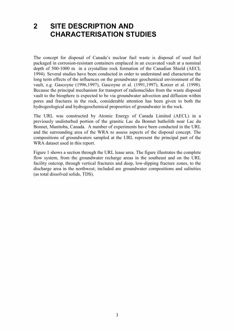
The concept for disposal of Canada’s nuclear fuel waste is disposal of used fuelpackaged in corrosion-resistant containers emplaced in an excavated vault at a nominaldepth of 500-1000 m in a crystalline rock formation of the Canadian Shield (AECL1994). Several studies have been conducted in order to understand and characterise thelong term effects of the influences on the groundwater geochemical environment of thevault, e.g. Gascoyne (1996,1997), Gascoyne et al. (1991,1997), Kotzer et al. (1998).Because the principal mechanism for transport of radionuclides from the waste disposalvault to the biosphere is expected to be via groundwater advection and diffusion withinpores and fractures in the rock, considerable attention has been given to both thehydrogeological and hydrogeochemical propoerties of groundwater in the rock.

The URL was constructed by Atomic Energy of Canada Limited (AECL) in apreviously undisturbed portion of the granitic Lac du Bonnet batholith near Lac duBonnet, Manitoba, Canada. A number of experiments have been conducted in the URLand the surrounding area of the WRA to assess aspects of the disposal concept. Thecompositions of groundwaters sampled at the URL represent the principal part of theWRA dataset used in this report.

Figure 1 shows a section through the URL lease area. The figure illustrates the completeflow system, from the groundwater recharge areas in the southeast and on the URLfacility outcrop, through vertical fractures and deep, low-dipping fracture zones, to thedischarge area in the northwest; included are groundwater compositions and salinities(as total dissolved solids, TDS).

4

Figure 1: Hydrogeologic section through the URL area. Groundwater compositionsand salinities (TDS) are based on pumping and sampling numerous boreholes in theWRA. The flow directions are based on pre- and post-excavation head distributions(Gascoyne, 1997).

The hydrogeologic section in Figure 1 shows that the near-surface groundwater inFracture Zone 3 (FZ3) and near-vertical fractures is typically Ca-HCO3 in composition.The groundwater evolves to a Na-HCO3 composition in the deep recharging portion ofthe underlying FZ2 and, as it flows up the dip of the fault toward the surface, dissolvedsalt content increases and the water becomes brackish. At greater depths in the URLarea, and elsewhere in the batholith, brackish and saline (Ca-Na-Cl or Na-Ca-Cl)groundwater predominates. This groundwater commonly has isotopic (δ2H - δ18O)characteristics that indicate recharge under cold-climate conditions (at least 8,000 yearsago) or, in the case of deeper, highly saline groundwater, under warm-climateconditions that are interpreted as being pre-glacial, i.e., >106 yr old (Gascoyne 1997;Gascoyne and Chan, 1992; Gascoyne, 1994). In some locations, this groundwater existsin isolated fracture zones of limited extent that are poorly connected to the near-surfacefracture network. However, in other locations, saline groundwater occurs at depths of<100 m in highly permeable fractures and is moving toward discharge locations at thesurface. An example of this phenomenon is shown on the left of Figure 1, wheregroundwater in FZ2 has a salinity of 1.5 g/L but is only 40 m below the surface.Hydraulic-head information shows that artesian conditions exist in FZ2 at this location,indicating that groundwater discharge is occurring at the base of the overburden abovethe subcrop of FZ2 (Gascoyne, 1997).

5

3 DATA COMPILATION AND EVALUATIONFOR FURTHER M3 MODELLING

The data set used in this work was compiled based on the published WRA data. Thefollowing additional information was added to the data (see Appendix 1):

• Data for meteoric precipitation

• An estimate of the isotopic composition of glacial melt-water

Based on literature studies, scatter plots of the data, and the spatial distribution of thesamples, the WRA data is believed to be appropriate for M3 modelling because:

• The analytical data comprise major components and isotopes (which togethercan reveal the information concerning the flow and reactions affecting thegroundwater)

• The water samples represent different depths

• The hydrogeological model supports the inference that mixing of different watertypes may occur.

• The water samples appear to be derived from different water types

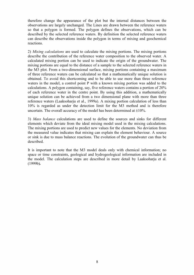
In addition a test was conducted on WRA data, where the possible influence of severalend-members on the groundwater and the potential for ambiguity were determined byusing a simple correlation test between water conservative constituents Cl and δ18O(Figure 2). If the correlation is low (as in this case) there are two or more end-membersinvolved in the groundwater system and a multivariate approach such as M3 can beemployed.

Figure 2: Scatter plot of Cl versus δ18O used to show that these water conservativeelements indicate low correlation implying a complex origin for WRA’s groundwaters.

-25

-20

-15

-10

0 10000 20000 30000 40000 50000 60000

Cl (m g/l)

de

l-1

8O

(S

MO

W)

7

4 DESCRIPTION OF M3 MODELLING

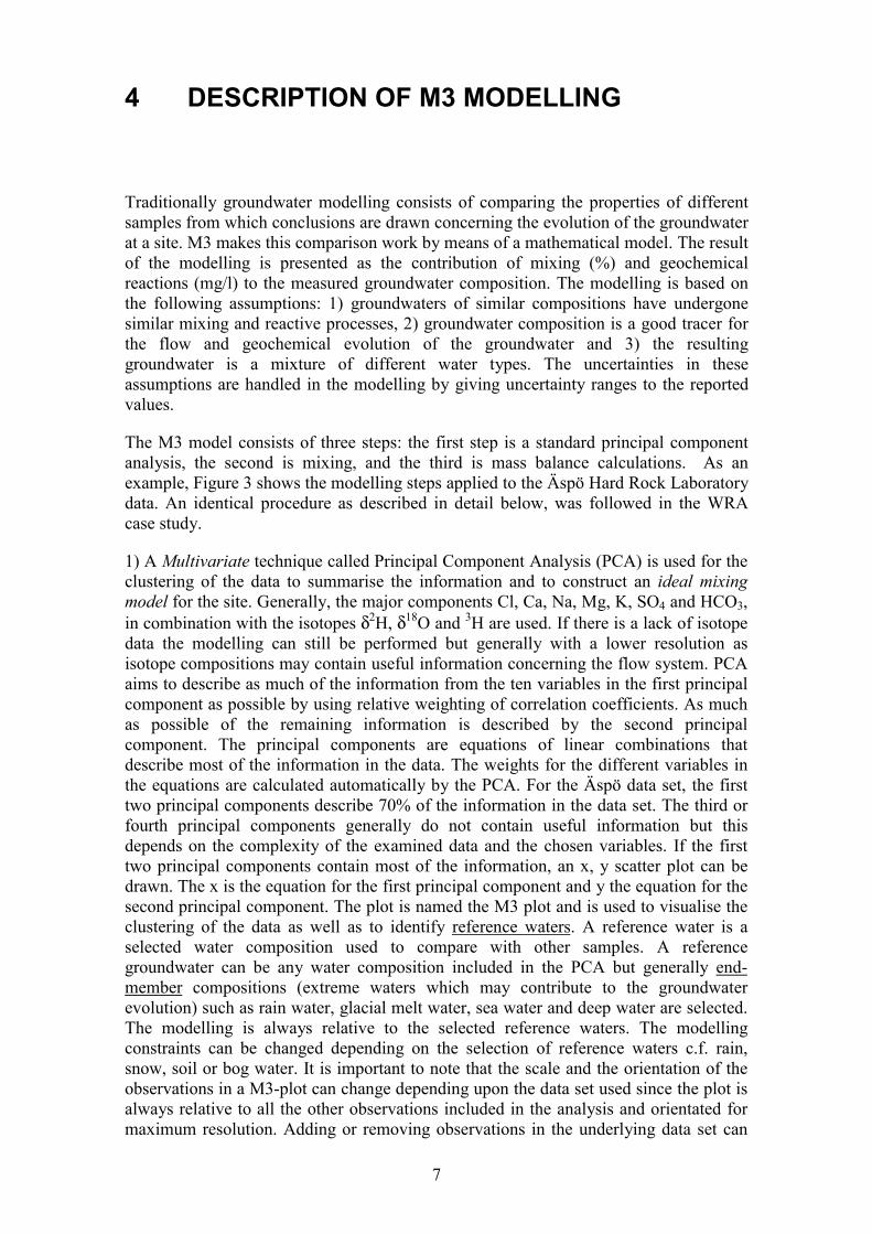
Traditionally groundwater modelling consists of comparing the properties of differentsamples from which conclusions are drawn concerning the evolution of the groundwaterat a site. M3 makes this comparison work by means of a mathematical model. The resultof the modelling is presented as the contribution of mixing (%) and geochemicalreactions (mg/l) to the measured groundwater composition. The modelling is based onthe following assumptions: 1) groundwaters of similar compositions have undergonesimilar mixing and reactive processes, 2) groundwater composition is a good tracer forthe flow and geochemical evolution of the groundwater and 3) the resultinggroundwater is a mixture of different water types. The uncertainties in theseassumptions are handled in the modelling by giving uncertainty ranges to the reportedvalues.

The M3 model consists of three steps: the first step is a standard principal componentanalysis, the second is mixing, and the third is mass balance calculations. As anexample, Figure 3 shows the modelling steps applied to the Äspö Hard Rock Laboratorydata. An identical procedure as described in detail below, was followed in the WRAcase study.

1) A Multivariate technique called Principal Component Analysis (PCA) is used for theclustering of the data to summarise the information and to construct an ideal mixingmodel for the site. Generally, the major components Cl, Ca, Na, Mg, K, SO4 and HCO3,in combination with the isotopes δ2H, δ18O and 3H are used. If there is a lack of isotopedata the modelling can still be performed but generally with a lower resolution asisotope compositions may contain useful information concerning the flow system. PCAaims to describe as much of the information from the ten variables in the first principalcomponent as possible by using relative weighting of correlation coefficients. As muchas possible of the remaining information is described by the second principalcomponent. The principal components are equations of linear combinations thatdescribe most of the information in the data. The weights for the different variables inthe equations are calculated automatically by the PCA. For the Äspö data set, the firsttwo principal components describe 70% of the information in the data set. The third orfourth principal components generally do not contain useful information but thisdepends on the complexity of the examined data and the chosen variables. If the firsttwo principal components contain most of the information, an x, y scatter plot can bedrawn. The x is the equation for the first principal component and y the equation for thesecond principal component. The plot is named the M3 plot and is used to visualise theclustering of the data as well as to identify reference waters. A reference water is aselected water composition used to compare with other samples. A referencegroundwater can be any water composition included in the PCA but generally end-member compositions (extreme waters which may contribute to the groundwaterevolution) such as rain water, glacial melt water, sea water and deep water are selected.The modelling is always relative to the selected reference waters. The modellingconstraints can be changed depending on the selection of reference waters c.f. rain,snow, soil or bog water. It is important to note that the scale and the orientation of theobservations in a M3-plot can change depending upon the data set used since the plot isalways relative to all the other observations included in the analysis and orientated formaximum resolution. Adding or removing observations in the underlying data set can

8

therefore change the appearance of the plot but the internal distances between theobservations are largely unchanged. The Lines are drawn between the reference watersso that a polygon is formed. The polygon defines the observations, which can bedescribed by the selected reference waters. By definition the selected reference waterscan describe the observations inside the polygon in terms of mixing and geochemicalreactions.

2) Mixing calculations are used to calculate the mixing portions. The mixing portionsdescribe the contribution of the reference water composition to the observed water. Acalculated mixing portion can be used to indicate the origin of the groundwater. Themixing portions are equal to the distance of a sample to the selected reference waters inthe M3 plot. From a two-dimensional surface, mixing portions containing a maximumof three reference waters can be calculated so that a mathematically unique solution isobtained. To avoid this shortcoming and to be able to use more than three referencewaters in the model, a control point P with a known mixing portion was added to thecalculations. A polygon containing, say, five reference waters contains a portion of 20%of each reference water in the centre point. By using this addition, a mathematicallyunique solution can be achieved from a two dimensional plane with more than threereference waters (Laaksoharju et al., 1999a). A mixing portion calculation of less than10% is regarded as under the detection limit for the M3 method and is thereforeuncertain. The overall accuracy of the model has been determined at ±10%.

3) Mass balance calculations are used to define the sources and sinks for differentelements which deviate from the ideal mixing model used in the mixing calculations.The mixing portions are used to predict new values for the elements. No deviation fromthe measured value indicates that mixing can explain the element behaviour. A sourceor sink is due to mass balance reactions. The evolution of the groundwater can thus bedescribed.

It is important to note that the M3 model deals only with chemical information; nospace or time constraints, geological and hydrogeological information are included inthe model. The calculation steps are described in more detail by Laaksoharju et al.(1999b).

9

Figure 3: Different steps in the M3 modelling; a) Data table containing groundwatercompositions. b) The principle of principal component analysis; seven groundwatersamples and their location in the multivariate space (VAR1-VAR5) and their projectionon the principal component 1 axis (PC1) are shown. Principal component analysis isused to summarise the data information and to obtain the maximum resolution of thedata set in order to construct an ideal mixing model for the site. c) The result of theprincipal component analysis showing principal components 1 and 2. d) Selection ofpossible reference waters - the other groundwater samples are compared to these, e)Mixing calculations – the linear distance of a sample to the reference waters e.g. theportions of meteoric water (%) are calculated in the figure for the selected ideal mixingmodel, the alternative model uses a new set of reference waters. f) Mass balancecalculations – the sources and sinks (mg/l) of carbonate (HCO3) are shown whichcannot be accounted for by using the ideal mixing model and therefore theinterpretation is that this is due to reactions. The M3 model is applied in this example todata from the Äspö Hard Rock Laboratory.

11

5 GENERAL UNCERTAINTIES IN THE M3MODELLING

The following errors can cause uncertainties in the M3 modelling:

1) Sampling errors caused by the effects from drilling, borehole activities, extensivepumping, hydraulic short circuiting of the borehole and uplifting (depressurization)of the water which may change the in-situ pH and Eh conditions of the sample.

2) Errors caused by inaccuracy of the analytical methods.

3) Conceptual errors such as incorrect general assumptions, selecting the wrongtype/number of end-members, and mixing samples that are not mixed.

4) Methodological errors such as oversimplification and bias in the model.

Most of the errors listed above are common for many types of modelling. The effects ofsampling errors are difficult to estimate since there is no in-situ sample fromundisturbed conditions. By labelling drilling water, the effects from drilling can beestimated. The borehole activities and short circuiting of the borehole may causeunnatural mixing of the groundwater. In the URL the water flow is towards the shaftwhich decreases or eliminates this kind of contamination. The depressurization of thewater can cause supersaturation of calcite which may change the Ca and HCO3 contentin the sample. The uncertainty due to sampling errors has been estimated/modelled to beof the order of ±10% from the undisturbed real values in most of the cases. Analyticalerrors for different elements vary but extensive comparison between differentlaboratories generally indicates a deviation of 1-5% in the values (Laaksoharju, 1999b).

When modelling with M3, the risk of conceptual errors occurs when makingassumptions such as groundwater composition is a good tracer for the flow system(which is generally the case). The water composition may not necessarily be a uniquetracer without a point source, such as labelled water in a tracer test. The accuracy istherefore much lower in M3 modelling than in a tracer test. On the other hand thetemporal space is much greater and therefore the information of larger value. Anotherassumption in M3 is that all the reference waters are mixed. This is necessary in order toconstruct an ideal mixing model and to be able to compare the samples. In reality thereare physical hindrances such as depth or geological structures, which may preventmixing from occurring, and therefore not every end-member necessarily contributes toevery water sample taken. Generally, three reference waters dominate in the M3calculations and the other ones are close to or below the detection limit for the method(a mixing portion of <10%. Uncertainty can occur from selecting the wrong number andtype of end-members. The selection of end-members or reference waters is a processwhich contains the following steps:

• Construct an independent paleo- or present-day conceptual model for the site tosuggest which type of water (glacial meltwater, brine, meteoric waters) may haveentered the bedrock. Here, additional information from Quaternary geology andfracture mineralogy may be helpful.

12

• Determine the minimum number and type of end-members needed to explain theobservations using the distribution of the samples in the PCA as a guide. This isgenerally an iterative process where different options are tested. New end-membercompositions guided by the conceptual model may be inserted in the data in order todescribe the observations. The scale (e.g. fracture scale or site scale) of themodelling determines which samples are to be included in the PCA and hence thenumber of end-members needed for the modelling.

• Test the mixing model to see how well it predicts water conservative elements suchas chloride, oxygen-18 and deuterium. Depending on the outcome of this test, themodel is rejected or accepted. If rejected, the scale of modelling is changed bydeleting observations and end-members. If the model is then accepted, anuncertainty range is calculated from the deviation of the water conservativeelements.

• Perform a feasibility test using different mixing proportions of the reference watersto reproduce the observed groundwater composition to build confidence in themodelling. Simple tests where (say) 50% meteoric water is mixed with 50% brinewater are included, to test that the water composition plots half way between thereference waters in the PCA.

Methodological errors in M3 can be due to the fact that complex groundwatercompositions (which may include as many as 10 variables) are summarised by a generalmodel where principal components 1 and 2 are used to summarise the information. Thereason for using the water composition described by the 10 variables rather thanconstructing a model from the water conservative tracers is that it is possible to have ahigher resolution in the PCA and a better chance of obtaining a unique solution. This isachieved by comparing groundwater compositions rather than that of 2 or 3conservative tracers. As mentioned in the previous chapter the mixing calculations aremathematically unique from the 2D surface in the PCA since a centre point P allowsmore than 3 reference samples to be used in the calculations. The third principalcomponent gathers generally around 10% of the groundwater information comparedwith the first and second principal components which contain around 70% of theinformation. Nevertheless, a sample may appear to be closer to a reference water in the2D surface than in a 3D surface involving the third principal component. This can affectthe accuracy of the mixing portion calculations.

In summary, the location of a sample on the PCA surface in M3 can be erroneousbecause of the sampling errors, analytical errors, conceptual errors and methodologicalerrors mentioned above. These difficulties are handled in M3 by stating the uncertaintyin the method as ±0.1 mixing units and the detection limit for the method as <10% of amixing portion.

13

6 M3 MODELLING OF WRA DATA

In the following sections the M3 model is applied to WRA data and, principally, datafrom groundwaters in the area of the URL. The modelling examples show selection ofreference waters, testing of the selected model, examples of reactions considered andcomparison of groundwater data from Canada and Scandinavia.

6.1 Selection of reference waters

In order to select reference waters for WRA data in M3 modelling the variables Na, K,Ca, Mg, Cl, SO4 HCO3, δ2H, 3H and δ18O were used in a principal component analysis.The results of the principal component analysis are shown in Figure 4a, b.

14

PC 1 = – 0.39[Na] + 0.03[K] + 0.25[Ca] + 0.09[Mg] – 0.39[HCO3] + 0.62[Cl] + 0.18[SO4] + 0.32[18O] + 0.22[2H]– 0.24[3H]

PC 2 = – 0.45[Na] + 0.12[K] + 0.07[Ca] + 0.04[Mg] – 0.02[HCO3] + 0.11[Cl] – 0.16[SO4] – 0.85[18O] + 0.14[2H]+ 0.02[3H]

Figure 4: a) The Principal Component plot based on the major components and waterconservative tracers Cl, deuterium, O18 and tritium. The numbers refer to groundwatersamples listed in Appendix 1. b) The reference waters Precipitation, Biogenic, Glacial,Saline and Brine have been selected from the data set used in the principal componentanalysis. A polygon is drawn between the samples in order to define the samples thatcan be described by the ideal mixing model. The equations for the first (PC1) andsecond (PC2) principal component describe the loadings from the different elements inthe model. The first and second principal components together describe 67% of thevariability or the information of the groundwater samples.

15

The selected reference waters for the current modelling are (analytical data are listed inAppendix 1):

• Brine reference water representing the brine type of water (Ca-Cl in composition)found in the rock matrix (Cl = 53,300 mg/l, Gascoyne et al. 1996).

• Saline reference water which represents saline groundwater (Na-Ca-Cl incomposition) found at depth in fracture zones in the WRA (Cl = 30,200 mg/l). Thistype of water is found in borehole WB1-7 (Gascoyne, 2000).

• Glacial reference water which has been determined as a glacial water with aassumed stable isotope value (δ18O = -25‰ SMOW) which indicate cold climaterecharge (Gascoyne, 2000).

• Biogenic reference water which represents water found in the borehole M12-159possibly altered by bacterial decomposition of organic material coupled with highCO2 production in combination with uptake near the surface. The water ischaracterised by a high content of HCO3 (255mg/l) but a rather low content of Ca(6.5 mg/l) which suggest a contribution from organic decomposition rather thancalcite dissolution.

• Precipitation reference water which represents a dilute infiltrating surface wateraffected by the precipitation from the 1960’s and therefore contains more tritium (3H= 90 TU) than modern rain (~20 TU).

6.2 Test of selected model

In the M3 modelling, selected reference waters are tested before an optimum model forthe site is chosen. Since M3 only compares groundwater samples at a site, the selectionof reference waters determines what type of modelling is to be performed and at whatscale. If only shallow groundwater is modelled, then there is no need to include brine asa reference water, but if the aim is to investigate the geochemical relationship betweendeeper waters and brine, a brine water composition has to be included in the modelling.The internal similarities/dissimilarities and the distribution of the samples in theprincipal component analysis generally help to select the appropriate number and typesof reference waters for M3 modelling. In any case, this generally requires several M3runs where models using different types and numbers of reference waters are tested. Thecriteria for a feasible model for a site is:

• The model can describe as many groundwater samples as possible• The mixing calculations are in general agreement with the hydrogeological

description of the groundwater and the conceptual/evolutionary model of thesite

• The deviations for the conservative constituents are reasonable• The deviations for the non-conservative elements make geochemical sense

In the example in Figure 5 the calculated values for WRA data are compared withmeasured values for different groundwater constituents. If the value is on the line thepredicted and measured value, coincide; if the value is above/under the line there is adeviation between the measured and predicted value. A deviation from the line for the

16

water conservative constituents such as Cl, oxygen-18 (δ18O) and deuterium (δ2H)indicates scatter in the model. A deviation for a reactive element such as HCO3 canindicate gain (values over the line) or losses (values under the line) associated withreactions. The results in Figure 5 can be used to check the feasibility of the selectedmodel for the site.

Figure 5: The WRA groundwaters are modelled to be a mixture of Precipitation,Biogenic, Glacial, Saline and Brine type of water as shown in the PCA (Figure a). Themodel can describe the water conservative elements (Cl, δ18O, δ2H) fairly well (note thedifferent scales in Figures b, c and d) and most of the observations are included in themodel (inside the polygon). A deviation for a reactive element such as Na, Ca, HCO3,SO4, Mg and K can indicate gain (values over the line) or loss (values under the line)associated with water rock interactions. The gain of tritium (3H) shows that some of theobservations have a higher tritium content (older water from nuclear testing) than theselected reference water (Precipitation). The loss of tritium for some samples canindicate radioactive decay.

17

6.3 Reactions considered

In theory thousands of chemical reactions could be written involving the water, solidsand gases in regional aquifers such as those at the URL site. There are eight maincategories of reactions and processes that control the chemistry of most groundwaters:precipitation-dissolution, acid-base, complexation, substitution-hydrolysis, oxidation-reduction, ion-filtration-osmosis, dissolution and exsolution of gases andsorption/desorption. Worldwide site modelling has revealed that the actual number ofreactions that dominate the groundwater chemistry is quite small (Alley, ed., 1993) suchas:

1) Introduction of CO2 gas in the unsaturated zone

2) Dissolution of calcite and dolomite, and precipitation of calcite

3) Cation exchange

4) Oxidation of pyrite and organic matter

5) Reduction of oxygen, nitrate, and sulphate, with production of sulphide

6) Reductive production of methane

7) Dissolution of gypsum, anhydrite and halite

8) Incongruent dissolution of primary silicates with formation of clays

In theory any effect from an inorganic/organic reaction can be traced by using M3. Inpractice the selection of reference waters, the validity of the ideal mixing model, modelerrors and the fact that a gain or a loss of an element can be due to several differentreactions give constraints on what kind of reactions can be traced with any accuracy.The M3 modelling is always relative to the selected reference waters and thereforedescribes always and only the net reactions which have to take place if these waters aremixed. The total reactions are the net reactions plus the reactions which have to takeplace to form the reference water (eg. Brine water).

Since much of the URL modelling in this work aimed at describing the groundwatersituation affected by the shaft construction this added an important constraint in themodelling, namely to focus on the fast short-term reactions in the modelling. Therelatively low temperature of the groundwater often hinders equilibrium from beingestablished between the groundwater and fracture minerals. Instead, recent research (eg,Pedersen and Karlsson, 1995; Stroes-Gascoyne and Gascoyne, 1998,) has shown thatmicrobes mediate in many reactions that otherwise would not take place. Organicmaterial (CH2O) generally plays an important role in these kinds of biogenic processes.The processes that are of major influence on the obtained groundwater at the URL siteare biological processes, redox reactions, calcite dissolution/precipitation and ionexchange. As an example, the effects from the following major reactions can bemodelled in detail with the M3 code:

18

1) Organic decomposition: This reaction is generally detected in the unsaturated zoneassociated with infiltrating precipitation water. This process consumes oxygen andadds reducing capacity to the groundwater according to the reaction: O2 + CH2O �CO2 + H2O. M3 reports a gain of HCO3 as a result of this reaction.

2) Organic redox reactions: An important redox reaction is reduction of iron IIIminerals through oxidation of organic matter: 4Fe(III) + CH2O + H2O � 4Fe2+ +4H+ + CO2. M3 reports a gain of HCO3 as a result of this reaction (this reaction wasnot modelled for the WRA data). This reaction takes place in the shallow part of thebedrock associated with influx of precipitation water.

3) Inorganic redox reaction: An example of an important inorganic redox reaction issulphide oxidation in the soil and of the fracture minerals containing pyriteaccording to the reaction: HS- + 2O2 � SO4

2- + H+. M3 reports a gain of SO4 as aresult of this reaction. This reaction generally takes place in the shallow part of thebedrock or in the case of a drawdown such as in the URL, at larger depths.

4) Dissolution and precipitation of calcite: There is generally a dissolution of calcitein the upper part and precipitation in the lower part of the bedrock according to thereaction: CO2 + CaCO3 � Ca2+ + 2HCO3

-. M3 reports both gains and losses of Caand HCO3 as a result of this reaction. This reaction can take place in anygroundwater type.

5) Ion exchange: Cation exchange with Na/Ca is a common reaction in groundwateraccording to the reaction: Na2X(s) + Ca2+ � CaX(s) + 2Na+, where X is a solidsubstrate such as a clay mineral. M3 reports a change in the Na/Ca ratios as a resultof this reaction. This reaction can take place in any groundwater type.

6) Sulphate reduction: Microbes can reduce sulphate to sulphide using organicsubstances in natural groundwater as reducing agents (Laaksoharju ed., 1995)according to the reaction: SO4

2- + 2CH2O + OH- � HS- + 2HCO3- + H2O. This

reaction is of importance since it may cause corrosion of copper canisters used in thefinal storage. Vigorous sulphate reduction is generally detected in association withmarine sediments that provide the organic material and the favourable salinityinterval for the microbes. M3 reports a loss of SO4 and a gain of HCO3 as a result ofthis reaction. This reaction modifies the groundwater composition by increasing theHCO3 content and decreasing the SO4 content. At the URL, this reaction does notoccur.

Of the above reactions only the reaction associated with organic decomposition(reaction#1) was modelled in this work (see section 7.3).

6.4 Comparison of groundwater data

M3 can be used for explorative data analysis where large data sets are examined. In thismodelling example the WRA data is compared by using principal component analysis inM3 with all the deep groundwater sampled in crystalline bedrock in Sweden andFinland (Figure 6). Groundwater samples which plot close to each other in the plot havea similar groundwater composition. A sample which plots close to one representingprecipitation is therefore assumed to contain more rain water or snow-melt than asample which plots close to one representing a brine type of water. The results showthat WRA data is similar to the shallow water (precipitation, and biogenic water (a

19

water type affected by organic reactions)) but is more affected by cold recharge water(glacial water) than seen in the Scandinavian data. The brine water is different from theScandinavian brine sample and not surprisingly, marine water has not affected the WRAdata to any large extent.

Figure 6: Principal component analysis in M3 is used to compare groundwater samplesfrom Scandinavia (Sweden and Finland) with Canadian WRA data. The Canadian dataare included in a principal component analysis together with Scandinavian data. Themodelling is based on the major components, stable isotopes and tritium values in morethan one thousand samples. Samples with a similar groundwater composition tend toform clusters in the plot. In order to help the comparison some extreme waters (end-members) such as marine water (sea water), precipitation (rain water), biogenic water(water affected by organic decomposition resulting in CO2 production and uptake),glacial water (cold recharge water from the last de-glaciation) and brine water (oldsaline water affected by long term water rock interactions with the rock matrix. The twoprincipal components together account for 65% of the variability, of the information inthe data set.

21

7 VISUALISATION OF M3 MODELLINGRESULTS

The measured values and the results from the M3 modelling can be illustrated ascontour plots for the site (Figures 7-15). These plots are based on 2D KRIGINGinterpolations using the computer code SURFER. The 2D interpolation in a NNW-SSEdirection was based on a total of 20 groundwater samples at the URL site. To reduceuncertainties, the cross-section was chosen where most of the sampling points werelocated. The samples are numbered in Figures according to observation number inAppendix 1.

The interpolation is uncertain at large depths (>500m) and in the corners of the cross-section where there are few or no observations. It is important to note that the water isflowing in fractures, but since there is a fracture network at the URL and, at large scale,the groundwater can mix, an interpolation method can be employed. The results of theinterpolation should be regarded as a potential map for a certain groundwater propertyto occur at a given bedrock location. The map has a high degree of accuracy only closeto the sampling points.

7.1 Water conservative tracers

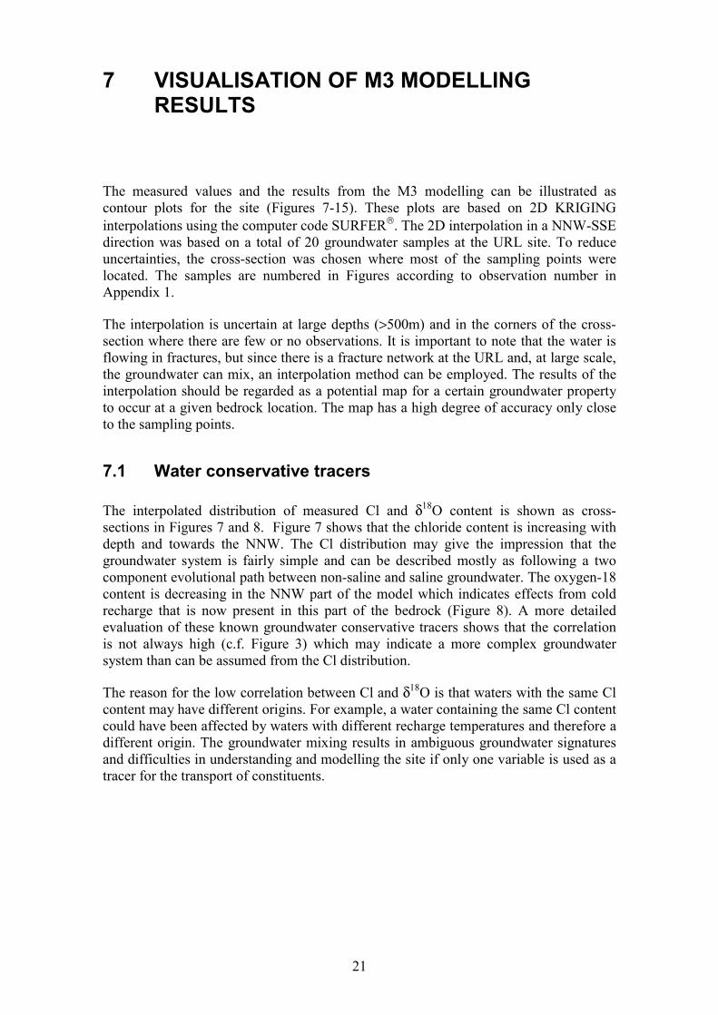
The interpolated distribution of measured Cl and δ18O content is shown as cross-sections in Figures 7 and 8. Figure 7 shows that the chloride content is increasing withdepth and towards the NNW. The Cl distribution may give the impression that thegroundwater system is fairly simple and can be described mostly as following a twocomponent evolutional path between non-saline and saline groundwater. The oxygen-18content is decreasing in the NNW part of the model which indicates effects from coldrecharge that is now present in this part of the bedrock (Figure 8). A more detailedevaluation of these known groundwater conservative tracers shows that the correlationis not always high (c.f. Figure 3) which may indicate a more complex groundwatersystem than can be assumed from the Cl distribution.

The reason for the low correlation between Cl and δ18O is that waters with the same Clcontent may have different origins. For example, a water containing the same Cl contentcould have been affected by waters with different recharge temperatures and therefore adifferent origin. The groundwater mixing results in ambiguous groundwater signaturesand difficulties in understanding and modelling the site if only one variable is used as atracer for the transport of constituents.

22

Figure 7: Visualisation of the measured Cl distribution at the URL site. The chloridecontent seems to be increasing with depth and towards NNW. The approximateassociated with the shaft construction, the major fracture zones, boreholes andsampling locations is shown.

23

Figure 8: Visualisation of the measured δ18O distribution at the URL site. The oxygen-18 content is decreasing in the NNW part of the model which may indicate effects fromcold recharge now present in this part of the bedrock. The approximate drawdownassociated with the shaft construction, the major fracture zones, boreholes andsampling locations is shown.

24

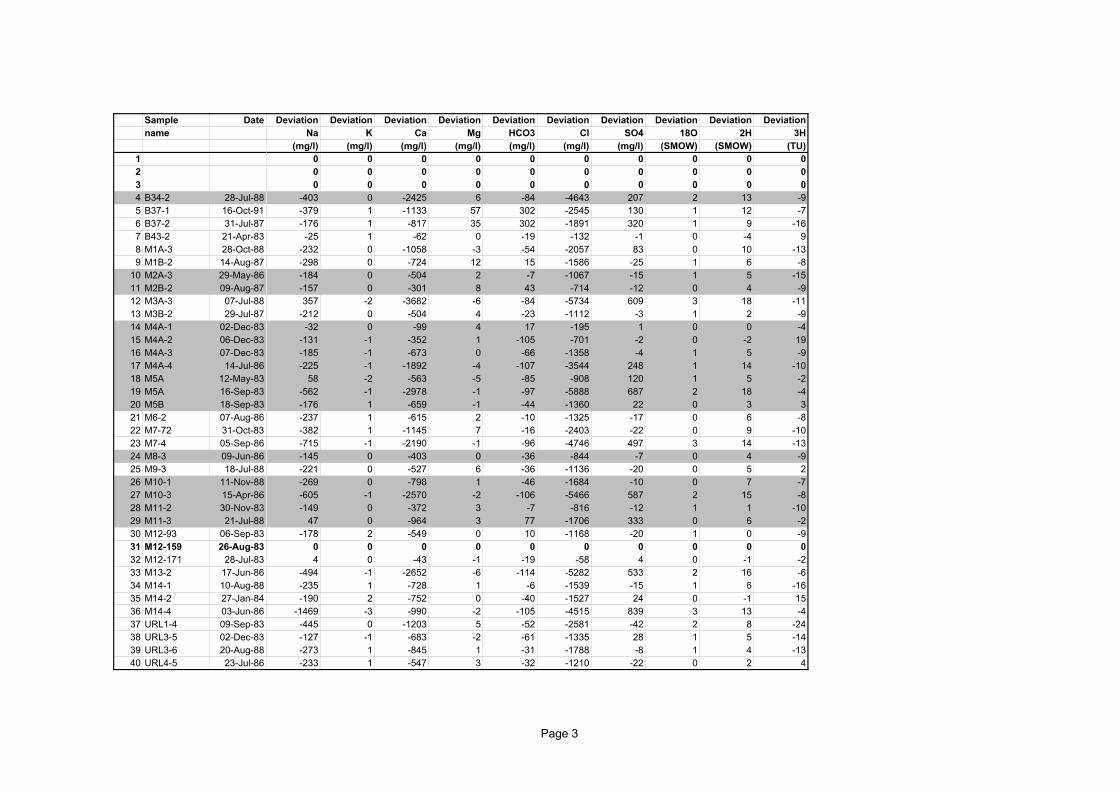
7.2 Mixing proportions

The results of M3 mixing calculations are shown as 2D cross-sections in Figures 9-13for the water types: precipitation, biogenic, glacial, saline and brine. The mixingportions always add up to 100% for all the samples. The construction of the URLcreated a large drawdown of the groundwater table around the elevator shaft. Thedrawdown resulted in changing inflow patterns and probably increased the mixing ofdifferent groundwater types.

Figure 9: Visualisation of the M3 calculated proportion (%) of precipitation water inthe bedrock at the URL site. The precipitation water content is high at the surface andgenerally decreases with depth. The content of 5-20% of precipitation water at largedepths in the boreholes M5A, M10 and URL 12 could be due to borehole activities (e.g.presence of residual drill-water). The approximate drawdown associated with the shaftconstruction, the major fracture zones, boreholes and sampling locations is shown.

25

Figure 10: Visualisation of the M3 calculated proportion (%) of biogenic water in thebedrock at the URL site. The biogenic water content is high in the upper part of thebedrock to a depth of 200m but also appears to exist at a greater depth (400m) close tothe shaft. This water type is mainly affected by decomposition of organic material anduptake of CO2 in the overburden which adds reducing capacity to the groundwater. Theapproximate drawdown associated with the shaft construction, the major fracturezones, boreholes and sampling locations is shown.

26

Figure 11: Visualisation of the M3 calculated proportion (%) of glacial water in thebedrock at the URL site. The glacial water content is high in the NNW part of thebedrock at larger depths than 400m. This water type is mainly affected by coldmeltwater from the last deglaciation which lowers the oxygen-18 content. Theapproximate drawdown associated with the shaft construction, the major fracturezones, boreholes and sampling locations is shown.

27

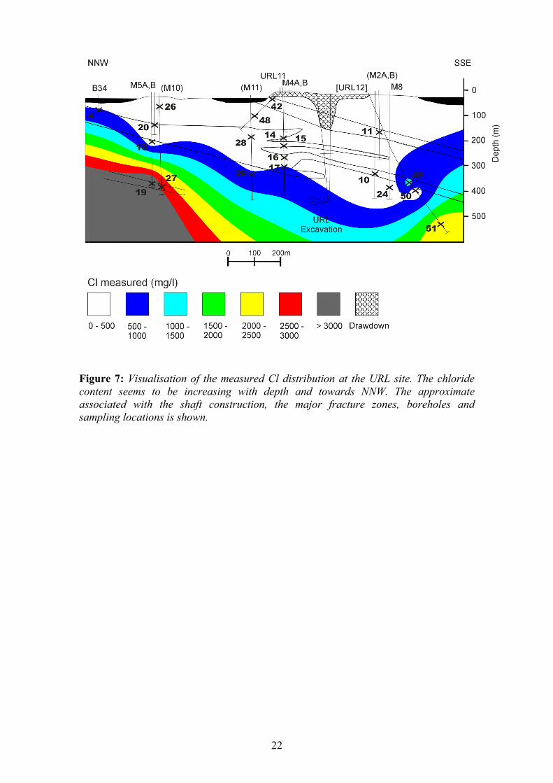
Figure 12: Visualisation of the M3 calculated proportion (%) of saline water in thebedrock at the URL site. The saline water content increase in the NNW and the SSE partof the bedrock at greater depths than 300m. This water type is mainly affected by longterm water rock interactions and is regarded as being pre-glacial. The approximatedrawdown associated with the shaft construction, the major fracture zones, boreholesand sampling locations is shown.

28

Figure 13: Visualisation of the M3 calculated proportion (%) of brine water in thebedrock at the URL site. The brine water content increases in the NNW and the SSEpart of the bedrock at greater depths than 300m. This water type is similar to that ofthe saline groundwater (Figure 12) except for the dominance of Ca, and may contributeto the salinity content in the saline groundwater. The high salinity of brine water isaffected by long term interactions with the rock matrix. The approximate drawdownassociated with the shaft construction, the major fracture zones, boreholes andsampling locations is shown.

The results of the M3 mixing calculations shown in Figures 9-13 indicate that the upperpart of the bedrock (0-100m) is dominated by precipitation type of water (100-40%). Atgreater depths (100-400m) the precipitation water is replaced by biogenic water (40-100%) which gradually consumes the oxygen of the groundwater, thus becomingreducing. At the depths of 300-600m and in the NNW part of the bedrock glacial water(40-80%) from the last deglaciation dominates. In the NNW and SSE part and at thesame depth interval as the glacial water (300-600m), the influence of saline (5-20%) andbrine (5-20%) types of water is detected. The draw-down from the shaft increased theportions of precipitation and biogenic water but seems to have flushed out historicalwaters such as glacial, saline and brine and hence the proportion of these waters werelow around the shaft. The occurrence and the distribution of water types are in goodagreement with earlier groundwater modelling of the site (e.g., Gascoyne, 1997).

29

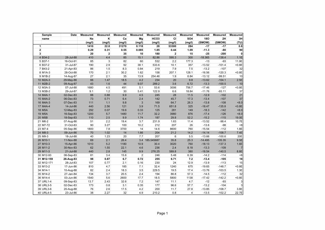
7.3 Mass-balance calculations

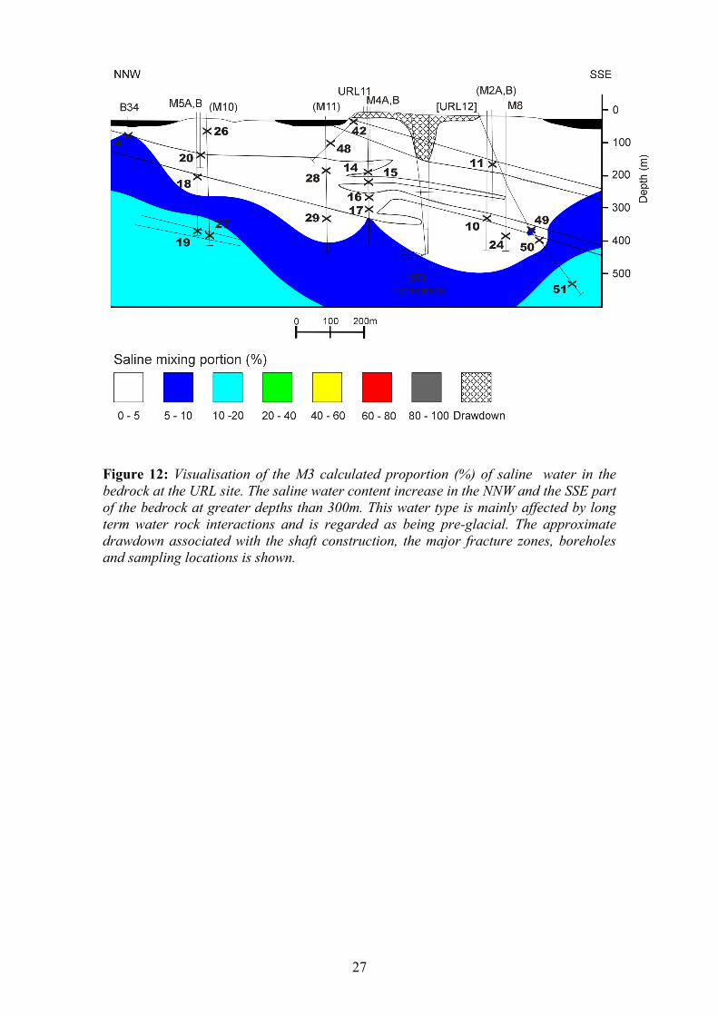
An example of results from the M3 mass-balance calculations is the behaviour of thecarbonate system at the URL site. Input of organic carbon into shallow groundwaterprovides a possible energy and carbon source for anaerobic respiration (see section 6.4).The measured HCO3 content and the calculated M3 deviation for this element is shownin Figures 14 and 15. The modelling indicates that there is a gain of HCO3 notaccounted for by mixing mainly associated with organic decomposition in the biogenicwater type and the enrichment of CO2 in near-surface sediments. At larger depths andin the NNW part of the site the modelling indicates a loss which may be due to calciteprecipitation. The mass-balance modelling for the carbonate system is in goodagreement with earlier groundwater modelling of the site (e.g., Gascoyne, 1997). Thecomplete M3 mass-balance modelling results for all the elements are reported inAppendix 1.

Figure 14: Visualisation of the measured HCO3 content at the URL site. Highconcentrations are detected at the depths 100-400m close to the URL shaft. The HCO3

content correlates with the biogenic water type (c.f. Figure 10). The approximatedrawdown associated with the shaft construction, the major fracture zones, boreholesand sampling locations is shown.

30

Figure 15: Visualisation of the M3 mass-balance calculations indicate a gain (positivevalue) of HCO3 not accounted for by mixing. The gain correlates with the biogenicwater type (c.f. Figure 10) and can be due to organic decomposition. At larger depthsand in the NNW part of the bedrock the modelling indicates a loss (negative value)which can indicate calcite precipitation. The approximate drawdown associated withthe shaft construction, the major fracture zones, boreholes and sampling locations areshown.

31

8 CONCLUSIONS

M3 modelling was applied to WRA hydrogeochemical data in order to determine itspotential as a modelling tool in the site description and evaluation process. The aim wasnot to perform a complete modelling of the WRA but rather to demonstrate if some ofthe results from previous work at the URL site could be repeated by using this newapproach.

In M3 modelling the assumption is that the groundwater chemistry is a result of mixingas well as water/rock reactions. The M3 model compares the groundwater compositionsfrom a site. The similarities and differences of the groundwater compositions are used toquantify the contribution from mixing and reactions on the measured data. In order toconstruct a reliable model, the method is used to summarise the information from thegroundwater data set by using the major components Cl, Ca, Na, Mg, K, SO4 and HCO3

in combination with the isotopes δ2H, δ18O and 3H. Initially, the method quantifies thecontribution from the flow system by comparing groundwater compositions toidentified reference waters. Subsequently, contributions from reactions are calculated.The model differs from many other standard models, which primarily use reactionsrather than mixing, to determine the groundwater evolution. The uncertainty in themethod is ±0.1 mixing units and the detection limit for the method is <10% of a mixingportion.

The modelled present-day groundwater conditions at the URL site consist of a mixturein varying degrees of the following water types: precipitation, biogenic, glacial, salineand brine. The results of the M3 mixing calculations indicate that the upper part of thebedrock (0-100m) is dominated by precipitation type of water (100-40%). At greaterdepths (100-400m) the precipitation water is replaced by biogenic water (40-100%)which gradually consumes the oxygen of the groundwater and becomes reducing. Atdepths 300-600m and in the NNW part of the bedrock glacial water (40-80%) from thelast deglaciation dominates. In the NNW and SSE part and at the same depth interval asthe glacial water (300-600m) the influences from saline (5-20%) and brine (5-20%) typeof waters are detected. The glacial water is a relatively thin lens and is underlain by thesaline, warm-climate water typical of WB 1-7 at ~1000m depth. The draw-down fromthe shaft increases the portions of precipitation and biogenic water but seemed to haveflushed out historical waters such as glacial, saline and brine from the near vicinity ofthe shaft. The M3 mass-balance modelling indicates that there is a gain of HCO3 notaccounted for by mixing probably associated with organic decomposition and CO2

uptake in the biogenic water type . At larger depths and in the NNW part of the bedrock,the modelling indicates a loss which may be due to calcite precipitation. The occurrenceand the distribution of water types and the mass-balance calculations for carbonate arein general agreement with earlier groundwater modelling of the site.

32

Although the M3 model is fairly new, with relatively few test cases, and requirescomplex multivariate mathematics, the major advantages of the model are:

• It is a mathematical tool which can be used to evaluate groundwater field dataand to support expert judgement of a site.

• The tool is not dependent on thermodynamic databases and can handle effects ofbiogenic reactions

• The results of mixing calculations can be compared/integrated withhydrodynamic models

• The numerical results of the modelling can be visualised and presented for non-expert use.

33

9 ACKNOWLEDGEMENTS

This study has been financed by Ontario Power Generation (OPG) and the SwedishNuclear Fuel and Waste Management Company (SKB). The support from Mark Jensen(OPG) and Peter Wikberg (SKB) are acknowledged.

35

10 REFERENCES

AECL 1994. Environmental Impact Statement on the Concept for Disposal of Canada’sNuclear Fuel Waste. Atomic Energy of Canada Limited Report AECL-10711/COG-93-1.

Alley W M (ed.), 1993. Regional groundwater quality. ISBN 0-442-00937-2. VanNostrand Reinhold, New York, USA, pp634.

Gascoyne, M. 2000. Hydrogeochemistry of the Whiteshell Research Area. OntarioPower Generation Report, in press.

Gascoyne M 1997 Evolution of Redox Conditions and Groundwater Composition inRecharge-Discharge Environments on the Canadian Shield, HydrogeologyJournal, Vol. 5, No. 3, 1997. Alley W M (ed.), 1993. Regional groundwaterquality. ISBN 0-442-00937-2. Van Nostrand Reinhold, New York, USA, pp634

Gascoyne, M., A. Bath and A. Gautschi. 1991. Hydrogeochemical monitoringrequirements for radioactive waste disposal in geological environments. In:Long Term Observations of the Geological Environment: Needs andTechniques, Proc. OECD/NEA Conf., Helsinki, Finland, 1991 September 9-11,93-108.

Gascoyne M and Thomas D, 1997, Impact of blasting on groundwater composition in afracture in Canada’s Underground Research Laboratory, Journal ofGeophysical Research, Vol. 102, No. B1, pages 573-584, 1997.

Gascoyne M, Frost L, Haveman S, Stroes-Gascoyne S, Thorne G, Vilks P, Clarke D,Ross J, Watson R, 1997, Chemical Evolution of Rapidly RechargingGroundwaters in Shield Environments, AECL-11814, COG-97-264-I.

Gascoyne, M., R.D. Ross and R.L. Watson. 1996. Highly saline pore fluids in the rockmatrix of a granitic batholith on the Canadian Shield. Abstract of paperpresented at International Geological Congress, Beijing, China, Aug. 4-14,1996

Gascoyne M, 1996, The geochemical environment of nuclear fuel waste disposal.Canadian Journal of Microbiology, Vol. 42, No. 4, pages 401-409, 1996.

Gascoyne M and Wuschke D, 1996, Gas migration through water-saturated, fracturedrock: results of a gas injection test, Journal of Hydrology 196 (1997) pages 76-98.

Gascoyne M, 1994, Isotopic and geochemical evidence for old groundwaters in agranite on the Canadian Shield: Radiochemical Acta, v. 58/59, p. 281-284.

Gascoyne M and Chan T, 1992, Comparision of numerically modelled groundwaterresidence time with isotopic age data, in Paleohydrogeological methods andtheir applications, Nuclear Energy Agency Workshop, 1992, Paris France:Proceedings, NEA/OECD, p. 199-206..

36

Gurban I, Laaksoharju M, Ledoux E, Made B, Salignac AL, 1998. Indications ofuranium transport around the reactor zone at Bagombé (Oklo). SKB TechnicalReport TR-98-06, Stockholm, Sweden.

Kotzer T, Gascoyne M, Mukai M, Ross J, Waito G, Milton G, Cornett R, 1998, 36Cl, 129Iand Noble Gas Isotope Systematics in Groundwaters from the Lac du BonnetBatholith, Manitoba, Canada. Radiochim. Acta 82, pages 313-318, 1998.

Laaksoharju M, Skårman C, Skårman E, 1999a. Multivariate Mixing and Mass-balance(M3) calculations, a new tool for decoding hydrogeochemical information.Applied Geochemistry Vol. 14, #7, 1999, Elsevier Science Ltd., pp861-871.

Laaksoharju M, Tullborg E-L, Wikberg P, Wallin B, Smellie J, 1999b.Hydrogeochemical conditions and evolution at Äspö HRL, Sweden. AppliedGeochemistry Vol. 14, #7, 1999, Elsevier Science Ltd., pp835-859.

Laaksoharju M, Gurban I, Andersson C, 1999c. Indications of the origin and evolutionof the groundwater at Palmottu. The Palmottu Natural Analogue Project. SKBTechnical Report TR 99-03, Stockholm, Sweden.

Laaksoharju, M; Wallin, B (eds.) 1997. Evolution of the groundwater chemistry at theÄspö Hard Rock Laboratory. Proceeding s of the second Äspö InternationalGeochemistry Workshop, June 6-7, 1995. SKB HRL International CooperationReport ICR 97-04. Laaksoharju, M (ed.), Gustafson G, Pedersen K, Rhén I,Skårman C, Tullborg E-L, Wallin B, Wikberg P, 1995. Sulphate reduction inthe Äspö HRL tunnel. SKB Technical Report TR 95-25, Stockholm, Sweden.

Pedersen K, Karlsson F, 1995. Investigation of subterranean bacteria - Theirimportance for performance assessment of radioactive waste disposal. In: SKBTechnical Report TR 95-10, Stockholm, Sweden.

Stroes-Gascoyne S and Gascoyne M, 1998, The Introduction of Microbial Nutrients intoA Nuclear Waste Disposal Vault during Excavation and Operation.Environmental Science & Technology, Vol. 32, No. 3, pages 317-326, 1998.

37

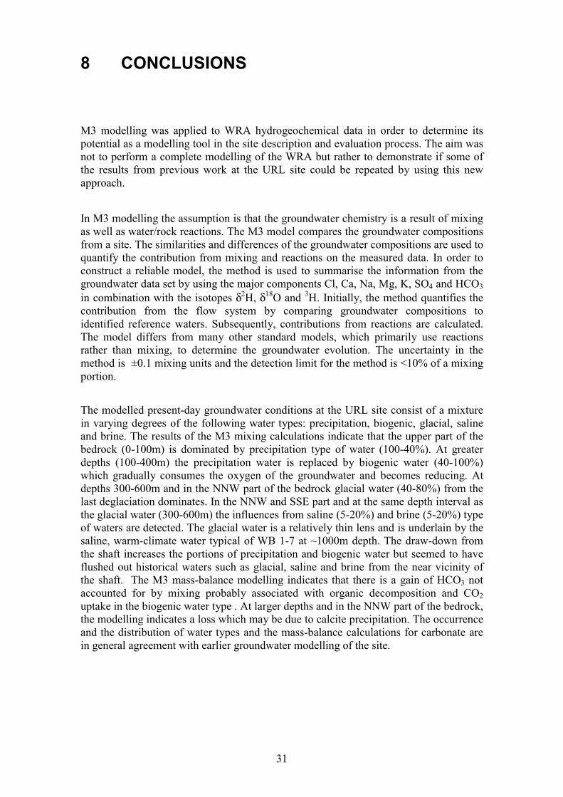
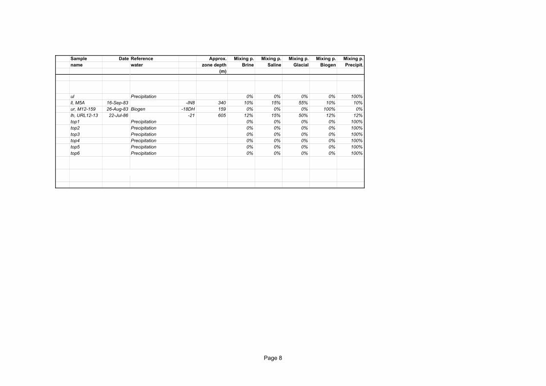
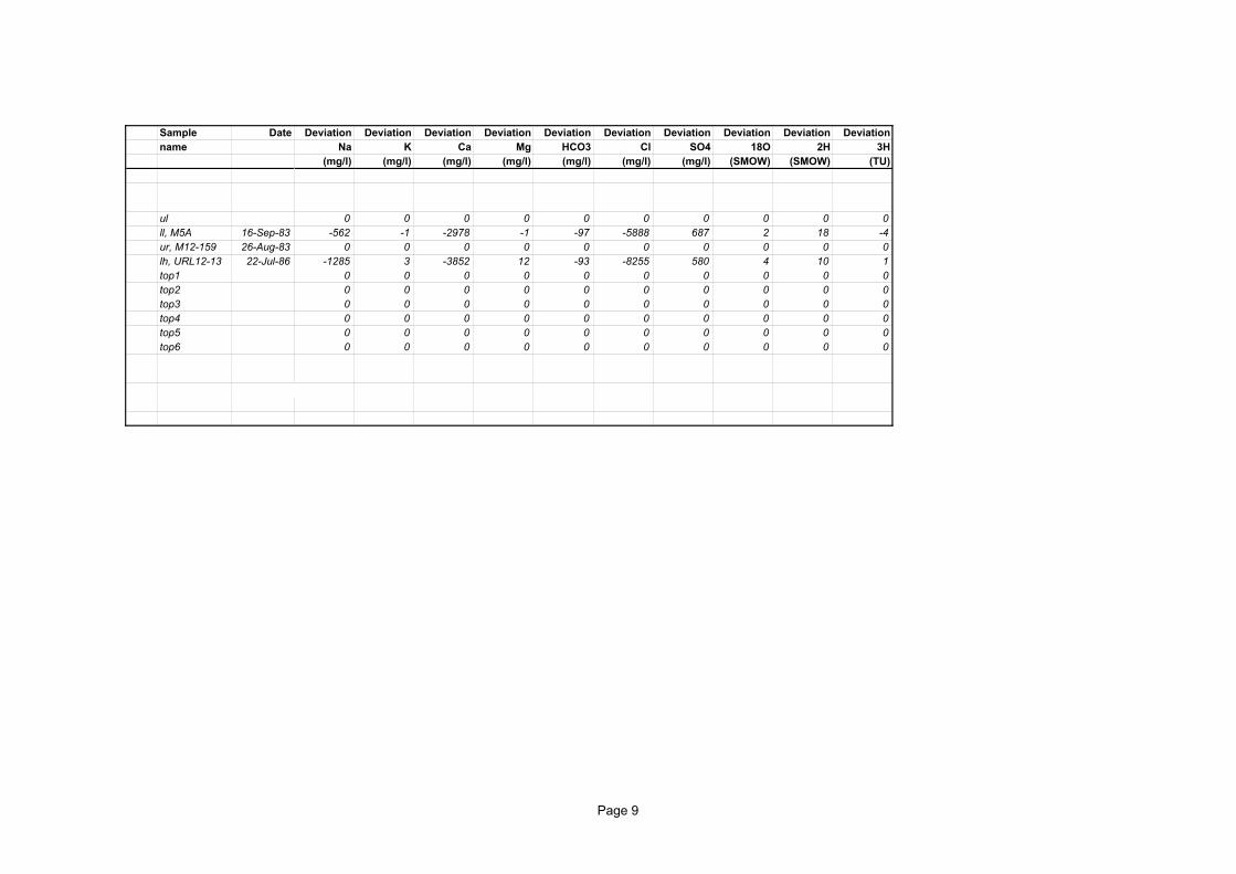
11 APPENDIX 1

Appendix 1 shows the WRA-data used in M3 modelling. The results from the M3mixing and mass-balance (deviation) calculations are listed. The numbers in the firstcolumn represent the row numbers used as index numbers in M3 modelling. Items inbold indicate the reference waters used in the different M3 calculations. Grey shadedcells mark samples used for interpolation/visualization (Kriging). Italics indicatessamples used as boundaries for the interpolations.

Sample Date Measured Measured Measured Measured Measured Measured Measured Measured Measured Measuredname Na K Ca Mg HCO3 Cl SO4 18O 2H 3H

(mg/l) (mg/l) (mg/l) (mg/l) (mg/l) (mg/l) (mg/l) (SMOW) (SMOW) (TU)1 1410 22.8 31270 0.118 28 53300 284 -17 -17 0.82 0.29 0.31 0.55 0.085 1.85 0.44 1.09 -11.3 -80 903 20 2 35 10 180 2 15 -25 -200 04 B34-2 28-Jul-88 410 4.4 85 15.1 82.86 595.3 300 -18.365 -138.4 1.1E5 B37-1 16-Oct-91 85 3 82 60 532 2.2 177.3 -13 -93 11.9E6 B37-2 31-Jul-87 190 2.9 92 38.1 533.6 10.1 357 -13.52 -101.4 <0.8E7 B43-2 21-Apr-83 86 1.5 8.3 0.84 219 7.9 7.5 -13.2 -107 328 M1A-3 28-Oct-88 170 2.1 30.2 1.62 158 207.1 128.1 -16.56 -120.3 <0.8E9 M1B-2 14-Aug-87 27 2.1 35 13.9 254.46 1.9 6.84 -13.12 -99.51 10

10 M2A-3 29-May-86 66 1.47 18.5 4.2 234 20 9.8 -13.62 -104.1 2.5E11 M2B-2 09-Aug-87 43 1.6 44 9.07 289.2 3.6 6.72 -13.3 -100.5 1012 M3A-3 07-Jul-88 1680 4.5 491 5.1 53.6 3006 756.7 -17.46 -127 <0.8E13 M3B-2 29-Jul-87 9.1 1.2 30 5.41 122.9 6.6 18.84 -11.76 -93.11 3714 M4A-1 02-Dec-83 88 0.88 9.9 4.5 245 28 11.5 -12.9 -102 2115 M4A-2 06-Dec-83 73 0.71 6.4 2.4 142 45.7 17.3 -13.4 -107 3716 M4A-3 07-Dec-83 111 1.1 9.8 3 169 64.7 26.3 -13.8 -108 <8.017 M4A-4 14-Jul-86 440 2.56 121 3.9 71.5 651.8 325 -18.47 -135.8 <0.8E18 M5A 12-May-83 292 0.07 19.6 0.33 125 281 149 -18.3 -142 <8.019 M5A 16-Sep-83 1200 5.7 1480 11.7 32.2 3980 876 -17.4 -126 <8.020 M5B 18-Sep-83 110 2.5 9.9 1.74 187 29.8 52.2 -15.2 -115 19.0E21 M6-2 07-Aug-86 51 2.2 19.4 3.7 231.9 1.63 11.4 -13.52 -98.4 10.7E22 M7-72 31-Oct-83 90 3.27 100 10.2 212 207 26 -13.6 -98 <823 M7-4 05-Sep-86 1800 7.8 3700 14 14.6 8600 760 -15.54 -112 1.8E24 M8-3 09-Jun-86 70 1.02 14 1.66 204 21.2 14.2 -14.14 -108.7 7.4E25 M9-3 18-Jul-88 40 1.23 20 7.7 207 6 5.5 -13.66 -100.6 20E26 M10-1 11-Nov-88 69 2.1 26.4 3.4 185.545687 35.8 25.3 -14.495 -105.35 9.5E27 M10-3 15-Apr-86 1010 5.2 1180 10.9 30.4 3020 760 -18.13 -137.3 1.6E28 M11-2 30-Nov-83 62 1.55 22.1 4.6 236 2.4 8.18 -13.3 -109 729 M11-3 21-Jul-88 440 2.8 145 9.9 276.25 589.8 380 -18.54 -140.5 8.8E30 M12-93 06-Sep-83 81 3.4 15.6 2 246 5.48 6.39 -14.2 -114 <831 M12-159 26-Aug-83 98 0.87 6.7 0.72 255 6.71 7.2 -13.4 -105 1832 M12-171 28-Jul-83 107 0.77 2.1 0.16 230 24 12.9 -13.9 -113 1533 M13-2 17-Jun-86 810 4.7 185 7.1 32.4 1240 675 -19.65 -148.7 <0.8E34 M14-1 10-Aug-88 82 2.4 18.3 3.5 229.5 19.5 17.4 -13.76 -103.5 1.3E35 M14-2 27-Jan-84 134 3.7 20.5 2.4 194 86.8 57.3 -14.5 -112 3236 M14-4 03-Jun-86 1540 5.6 2600 17.7 18.5 5800 1138 -17.42 -142.2 <0.8E37 URL1-4 09-Sep-83 13.7 2.43 32.6 7.2 147 11.1 4.7 -12 -93 338 URL3-5 02-Dec-83 173 0.8 3.1 0.35 177 96.6 57.7 -13.2 -104 339 URL3-6 20-Aug-88 76 2.6 17.5 4.2 200 11.7 27.8 -13.85 -108.7 3.8E40 URL4-5 23-Jul-86 38 2.27 32 4.9 210.2 0.8 4 -13.5 -102.2 22.7E

Page 1

Sample Datename

1234 B34-2 28-Jul-885 B37-1 16-Oct-916 B37-2 31-Jul-877 B43-2 21-Apr-838 M1A-3 28-Oct-889 M1B-2 14-Aug-87

10 M2A-3 29-May-8611 M2B-2 09-Aug-8712 M3A-3 07-Jul-8813 M3B-2 29-Jul-8714 M4A-1 02-Dec-8315 M4A-2 06-Dec-8316 M4A-3 07-Dec-8317 M4A-4 14-Jul-8618 M5A 12-May-8319 M5A 16-Sep-8320 M5B 18-Sep-8321 M6-2 07-Aug-8622 M7-72 31-Oct-8323 M7-4 05-Sep-8624 M8-3 09-Jun-8625 M9-3 18-Jul-8826 M10-1 11-Nov-8827 M10-3 15-Apr-8628 M11-2 30-Nov-8329 M11-3 21-Jul-8830 M12-93 06-Sep-8331 M12-159 26-Aug-8332 M12-171 28-Jul-8333 M13-2 17-Jun-8634 M14-1 10-Aug-8835 M14-2 27-Jan-8436 M14-4 03-Jun-8637 URL1-4 09-Sep-8338 URL3-5 02-Dec-8339 URL3-6 20-Aug-8840 URL4-5 23-Jul-86

Reference Approx. Mixing p. Mixing p. Mixing p. Mixing p. Mixing p.water zone depth Brine Saline Glacial Biogen Precipit.

(m)End-member brine 100% 0% 0% 0% 0%Precipitation 0% 0% 0% 0% 100%Glacial melt-water 0% 0% 100% 0% 0% -4 40 6% 6% 57% 24% 6%

-5 22 3% 3% 4% 87% 3%-3 45 2% 2% 9% 84% 2%-3 123 0% 0% 0% 93% 6%-7 265 3% 3% 31% 61% 3%-3 75 2% 2% 3% 92% 2%-4 310 1% 1% 6% 90% 1%-5 150 1% 1% 1% 96% 2%-4 375 10% 10% 56% 13% 10%-1 120 1% 1% 1% 56% 40%

-15 180 0% 0% 0% 89% 10%-2 215 1% 1% 2% 96% 1%-7 260 2% 2% 10% 85% 2%-6 310 5% 5% 53% 32% 5%-3 165 1% 1% 47% 49% 1%

-IN8 340 10% 15% 55% 10% 10%-IN9 120 2% 2% 16% 79% 2%

-5 110 2% 2% 2% 93% 2%-DH 72 3% 3% 6% 85% 3%-11 390 13% 21% 40% 13% 13%-7 360 1% 1% 10% 87% 1%-3 230 1% 1% 3% 93% 1%-7 50 2% 2% 11% 83% 2%-2 410 8% 13% 62% 8% 8%

-12 140 1% 1% 6% 91% 1%-4 290 3% 3% 48% 44% 3%

-DH 93 1% 1% 11% 84% 1%Biogen -18DH 159 0% 0% 0% 100% 0%

-15DH 171 0% 0% 7% 92% 0%-5 250 6% 11% 71% 6% 6%-4 50 2% 2% 7% 87% 2%

-13 105 2% 2% 9% 85% 2%-4 370 4% 27% 61% 4% 4%

-24 110 3% 3% 3% 75% 15%-1 120 2% 2% 7% 88% 2%-9 140 2% 2% 11% 82% 2%

-10 65 1% 1% 1% 94% 2%

Page 2

Sample Datename

1234 B34-2 28-Jul-885 B37-1 16-Oct-916 B37-2 31-Jul-877 B43-2 21-Apr-838 M1A-3 28-Oct-889 M1B-2 14-Aug-87

10 M2A-3 29-May-8611 M2B-2 09-Aug-8712 M3A-3 07-Jul-8813 M3B-2 29-Jul-8714 M4A-1 02-Dec-8315 M4A-2 06-Dec-8316 M4A-3 07-Dec-8317 M4A-4 14-Jul-8618 M5A 12-May-8319 M5A 16-Sep-8320 M5B 18-Sep-8321 M6-2 07-Aug-8622 M7-72 31-Oct-8323 M7-4 05-Sep-8624 M8-3 09-Jun-8625 M9-3 18-Jul-8826 M10-1 11-Nov-8827 M10-3 15-Apr-8628 M11-2 30-Nov-8329 M11-3 21-Jul-8830 M12-93 06-Sep-8331 M12-159 26-Aug-8332 M12-171 28-Jul-8333 M13-2 17-Jun-8634 M14-1 10-Aug-8835 M14-2 27-Jan-8436 M14-4 03-Jun-8637 URL1-4 09-Sep-8338 URL3-5 02-Dec-8339 URL3-6 20-Aug-8840 URL4-5 23-Jul-86

Deviation Deviation Deviation Deviation Deviation Deviation Deviation Deviation Deviation DeviationNa K Ca Mg HCO3 Cl SO4 18O 2H 3H

(mg/l) (mg/l) (mg/l) (mg/l) (mg/l) (mg/l) (mg/l) (SMOW) (SMOW) (TU)0 0 0 0 0 0 0 0 0 00 0 0 0 0 0 0 0 0 00 0 0 0 0 0 0 0 0 0

-403 0 -2425 6 -84 -4643 207 2 13 -9-379 1 -1133 57 302 -2545 130 1 12 -7-176 1 -817 35 302 -1891 320 1 9 -16-25 1 -62 0 -19 -132 -1 0 -4 9

-232 0 -1058 -3 -54 -2057 83 0 10 -13-298 0 -724 12 15 -1586 -25 1 6 -8-184 0 -504 2 -7 -1067 -15 1 5 -15-157 0 -301 8 43 -714 -12 0 4 -9357 -2 -3682 -6 -84 -5734 609 3 18 -11

-212 0 -504 4 -23 -1112 -3 1 2 -9-32 0 -99 4 17 -195 1 0 0 -4

-131 -1 -352 1 -105 -701 -2 0 -2 19-185 -1 -673 0 -66 -1358 -4 1 5 -9-225 -1 -1892 -4 -107 -3544 248 1 14 -10

58 -2 -563 -5 -85 -908 120 1 5 -2-562 -1 -2978 -1 -97 -5888 687 2 18 -4-176 1 -659 -1 -44 -1360 22 0 3 3-237 1 -615 2 -10 -1325 -17 0 6 -8-382 1 -1145 7 -16 -2403 -22 0 9 -10-715 -1 -2190 -1 -96 -4746 497 3 14 -13-145 0 -403 0 -36 -844 -7 0 4 -9-221 0 -527 6 -36 -1136 -20 0 5 2-269 0 -798 1 -46 -1684 -10 0 7 -7-605 -1 -2570 -2 -106 -5466 587 2 15 -8-149 0 -372 3 -7 -816 -12 1 1 -10

47 0 -964 3 77 -1706 333 0 6 -2-178 2 -549 0 10 -1168 -20 1 0 -9

0 0 0 0 0 0 0 0 0 04 0 -43 -1 -19 -58 4 0 -1 -2

-494 -1 -2652 -6 -114 -5282 533 2 16 -6-235 1 -728 1 -6 -1539 -15 1 6 -16-190 2 -752 0 -40 -1527 24 0 -1 15

-1469 -3 -990 -2 -105 -4515 839 3 13 -4-445 0 -1203 5 -52 -2581 -42 2 8 -24-127 -1 -683 -2 -61 -1335 28 1 5 -14-273 1 -845 1 -31 -1788 -8 1 4 -13-233 1 -547 3 -32 -1210 -22 0 2 4

Page 3

Sample Date Measured Measured Measured Measured Measured Measured Measured Measured Measured Measuredname Na K Ca Mg HCO3 Cl SO4 18O 2H 3H

(mg/l) (mg/l) (mg/l) (mg/l) (mg/l) (mg/l) (mg/l) (SMOW) (SMOW) (TU)41 URL5-4 11-May-82 145 2.76 7.5 1.61 220 84 34 -14.5 -111 <842 URL6 12-Jul-83 280 4.33 21.5 3.5 147 336 76 -15.2 -116 9243 URL7 22-Aug-82 23.4 1.98 26.5 12 208 1.1 7.5 -13.2 -98 3344 URL8-7 14-Aug-84 81 2 22.2 4.3 219 31 17.2 -14.4 -108 <845 URL10-3 09-May-86 22.1 2.01 35.4 10 185 1.46 16.4 -14.11 -109.1 18.3E46 URL10-6 24-Jun-86 172 2.9 35 3.9 182 155 98.6 -15.95 -118.4 3.5E47 URL11-3 20-Jul-84 10.6 2.31 49 8.3 181 5.1 22.6 -13.2 -107 5148 URL11-7 29-Nov-88 72 1.5 25.1 5.5 221.7 4.3 40.2 -13.75 -100.7 23.0E49 URL12-10 11-Apr-90 735 2.62 156 3.44 51.7 1246 216.8 -17.53 -127.55 <0.8E50 URL12-11 11-Sep-86 93 3.3 37 3.6 118.6 96 61 -13.28 -103 21.5E51 URL12-13 22-Jul-86 530 10.2 1070 25 31.9 2454 776 -15.41 -127.7 14.2E52 URL14 23-Jul-87 1800 4.9 710 8.05 14.5 3389 732 -16.55 -120.9 <0.8E53 URL15-1 26-May-88 200 5.4 30 3.8 222 190.5 93 -13.55 -104.7 <6.054 URL16-4 24-Aug-88 52 3.5 35.3 8.5 184 17.7 36.6 -11.15 -93 20.5E55 WA1-1 10-Jul-87 9.3 8 40 2.34 118.5 6.9 3.12 -12.03 -99.15 1956 WA1-2 29-Jun-87 26 4.5 44 9.7 256 1.9 1.7 -11.29 -95.2 11.1E57 WA1-3 08-Nov-87 84 2.45 35 5.5 321.2 10.8 11.4 -13.81 -104.6 11.1E58 WA1-5 18-Mar-88 1100 12 1714 44.4 35 3800 1323 -19.04 -139.6 1.3E59 WB1-1 05-Jun-87 80 4 43 8.3 251.6 56.8 21.3 -12.42 -94.5 17.3E60 WB1-2 05-Jun-87 260 6 69 10.3 156.7 300 272 -13.47 -104.7 10.8E61 WB1-4 05-Aug-87 5200 15 725 11.7 16.5 9797 1320 -11.3 -88.85 13.3E62 WB1-5 06-Oct-87 3100 17 3590 37 14 10780 990 -14.12 -105.3 7.3E63 WB1-7 30-May-88 11000 24 8410 51.1 9.9 30200 1040 -12.96 -94.35 2.1E64 WB2-20 12-Mar-91 4360 14.25 10540 34.2 20.1 27900 835 -15.4 -102 <0.8E65 WD1-110 03-Sep-88 81 1.8 12.3 2.94 241.3 2.8 11.2 -13.82 -106.8 1666 WD2-72 01-Sep-88 59 2.6 28 5.5 255 1.6 11.7 -13.45 -103.4 10.2E67 WD3-895 14-Sep-88 1900 7.9 4300 40 26.2 11390 492 -15.62 -113.15 5.2E68 WG2-2 15-May-87 70 2.6 13.4 2.71 218.5 3.3 7.4 -13.04 -100.3 9.0E69 WN1-8 24-May-87 1400 8 1150 53.3 73 3480 770 -16.18 -117.4 2.6E70 WN3 20-Aug-79 160 3.3 25.4 11.1 328 119 82 -16.2 -122 <871 WN4-6 08-May-87 1400 9 1370 60.8 60.8 3880 890 -16.54 -120.6 5972 WN4-13 11-Dec-89 4890 10.5 2687 25.5 15 11091 1393.1 -15.95 -116.5 <0.8E73 WN8 26-Aug-88 1060 5.3 740 39.8 85.2 2581 630 -16.78 -124.5 1.6E74 WN10-3 09-Dec-88 770 5.6 289 27 71 1350 700 -17.87 -132.4 <0.8E75 WN10-4 26-Mar-87 1330 8.7 910 66 27 2909 1400 -18.14 -131.3 2.3E76 WN11-17 09-Dec-86 6800 19.1 4930 26.7 19.6 18944 1105 -14.12 -109.1 3.0E

Page 4

Sample Datename

41 URL5-4 11-May-8242 URL6 12-Jul-8343 URL7 22-Aug-8244 URL8-7 14-Aug-8445 URL10-3 09-May-8646 URL10-6 24-Jun-8647 URL11-3 20-Jul-8448 URL11-7 29-Nov-8849 URL12-10 11-Apr-9050 URL12-11 11-Sep-8651 URL12-13 22-Jul-8652 URL14 23-Jul-8753 URL15-1 26-May-8854 URL16-4 24-Aug-8855 WA1-1 10-Jul-8756 WA1-2 29-Jun-8757 WA1-3 08-Nov-8758 WA1-5 18-Mar-8859 WB1-1 05-Jun-8760 WB1-2 05-Jun-8761 WB1-4 05-Aug-8762 WB1-5 06-Oct-8763 WB1-7 30-May-8864 WB2-20 12-Mar-9165 WD1-110 03-Sep-8866 WD2-72 01-Sep-8867 WD3-895 14-Sep-8868 WG2-2 15-May-8769 WN1-8 24-May-8770 WN3 20-Aug-7971 WN4-6 08-May-8772 WN4-13 11-Dec-8973 WN8 26-Aug-8874 WN10-3 09-Dec-8875 WN10-4 26-Mar-8776 WN11-17 09-Dec-86

Reference Approx. Mixing p. Mixing p. Mixing p. Mixing p. Mixing p.water zone depth Brine Saline Glacial Biogen Precipit.

(m)-43 100 2% 2% 12% 82% 2%-25 270 1% 1% 1% 94% 2%-24 60 1% 1% 1% 81% 15%-6 230 2% 2% 11% 84% 2%-2 80 2% 2% 11% 83% 2%-7 250 3% 3% 26% 66% 3%-1 45 1% 1% 1% 85% 12%-7 135 1% 1% 2% 95% 1%

-19 390 6% 6% 45% 38% 6%-13 430 3% 3% 6% 84% 3%-21 605 12% 15% 50% 12% 12%-8 280 12% 12% 52% 13% 12%-4 125 4% 4% 9% 80% 4%-1 85 2% 2% 2% 52% 41%-3 150 5% 5% 5% 63% 22%-8 240 2% 2% 2% 57% 36%-8 320 1% 1% 2% 96% 1%-7 630 - - - - - -5 130 2% 2% 2% 66% 28%-6 230 6% 6% 15% 67% 6%

-SW10 540 15% 37% 19% 15% 15%-21 630 9% 45% 30% 9% 9%

Saline -7 1000 0% 100% 0% 0% 0%-12 725 8% 63% 15% 8% 8%-2 100 1% 1% 5% 93% 1%-5 65 1% 1% 3% 92% 1%

-10 810 12% 26% 38% 12% 12%-8 130 2% 2% 2% 91% 3%

-17 380 8% 24% 51% 8% 8%-90 90 1% 1% 23% 73% 1%-8 370 10% 22% 47% 10% 10%

-20 650 3% 49% 42% 3% 3%-T4 315 10% 13% 56% 10% 10%

-4 245 9% 12% 62% 9% 9%-3 320 - - - - -

-15 1000 4% 66% 21% 4% 4%

Page 5

Sample Datename

41 URL5-4 11-May-8242 URL6 12-Jul-8343 URL7 22-Aug-8244 URL8-7 14-Aug-8445 URL10-3 09-May-8646 URL10-6 24-Jun-8647 URL11-3 20-Jul-8448 URL11-7 29-Nov-8849 URL12-10 11-Apr-9050 URL12-11 11-Sep-8651 URL12-13 22-Jul-8652 URL14 23-Jul-8753 URL15-1 26-May-8854 URL16-4 24-Aug-8855 WA1-1 10-Jul-8756 WA1-2 29-Jun-8757 WA1-3 08-Nov-8758 WA1-5 18-Mar-8859 WB1-1 05-Jun-8760 WB1-2 05-Jun-8761 WB1-4 05-Aug-8762 WB1-5 06-Oct-8763 WB1-7 30-May-8864 WB2-20 12-Mar-9165 WD1-110 03-Sep-8866 WD2-72 01-Sep-8867 WD3-895 14-Sep-8868 WG2-2 15-May-8769 WN1-8 24-May-8770 WN3 20-Aug-7971 WN4-6 08-May-8772 WN4-13 11-Dec-8973 WN8 26-Aug-8874 WN10-3 09-Dec-8875 WN10-4 26-Mar-8776 WN11-17 09-Dec-86

Deviation Deviation Deviation Deviation Deviation Deviation Deviation Deviation Deviation DeviationNa K Ca Mg HCO3 Cl SO4 18O 2H 3H

(mg/l) (mg/l) (mg/l) (mg/l) (mg/l) (mg/l) (mg/l) (SMOW) (SMOW) (TU)-155 1 -694 -1 -13 -1378 3 0 4 -8

18 3 -528 2 -96 -812 51 -2 -11 73-240 1 -569 10 -1 -1245 -18 0 3 5-197 0 -604 2 -17 -1272 -11 0 5 -9-306 0 -754 7 -48 -1647 -17 1 4 1-240 1 -1072 -1 -33 -2151 53 1 8 -11-190 1 -329 7 -38 -784 4 0 -5 25-174 0 -470 4 -23 -1030 17 0 4 5

-6 -1 -2085 -4 -129 -3434 133 1 13 -11-402 1 -1287 1 -108 -2679 10 1 4 3

-1285 3 -3852 12 -93 -8255 580 4 10 1315 -2 -3984 -3 -116 -6451 567 3 18 -13

-337 3 -1438 0 0 -2886 37 1 4 -12-300 2 -930 7 46 -2008 0 2 2 -26-668 5 -1933 -1 -53 -4136 -68 2 0 -12-298 3 -815 8 105 -1799 -32 2 1 -32-74 1 -175 4 72 -423 -3 0 2 -7 - - - - - - - - - -

-246 2 -796 7 78 -1703 -12 1 4 -19-547 2 -2300 5 -44 -4670 186 2 7 -7931 2 -6946 -9 -64 -9100 892 4 14 -3

-1951 4 -2863 11 -68 -7291 496 3 13 -30 0 0 0 0 0 0 0 0 0

-2643 -3 2922 1 -34 4991 160 0 2 -9-110 1 -313 1 -4 -671 -7 0 2 -1-211 1 -550 4 13 -1206 -15 0 3 -8

-1162 -2 -1623 23 -79 -2830 180 2 12 -8-242 1 -704 1 -18 -1498 -23 1 4 -10

-1370 -1 -3472 36 -45 -8169 489 3 24 -7-71 2 -484 8 100 -930 57 0 4 -6

-1180 0 -3734 45 -55 -8273 624 2 15 47-602 -3 -2364 -4 -74 -5341 864 2 20 -3-589 -2 -3600 27 -46 -6925 451 3 21 -10-720 -1 -3455 14 -66 -6940 538 3 20 -9

- - - - - - - - - - -496 2 -1941 -9 -38 -3179 406 2 4 -3

Page 6

Sample Date Measured Measured Measured Measured Measured Measured Measured Measured Measured Measuredname Na K Ca Mg HCO3 Cl SO4 18O 2H 3H

(mg/l) (mg/l) (mg/l) (mg/l) (mg/l) (mg/l) (mg/l) (SMOW) (SMOW) (TU)

Boundarie conditions

ul 0.29 0.31 0.55 0.085 1.85 0.44 1.09 -11.3 -80 90ll, M5A 16-Sep-83 1200 5.7 1480 11.7 32.2 3980 876 -17.4 -126 8ur, M12-159 26-Aug-83 98 0.87 6.7 0.72 255 6.71 7.2 -13.4 -105 18lh, URL12-13 22-Jul-86 530 10.2 1070 25 31.9 2454 776 -15.41 -127.7 14.2top1 0.29 0.31 0.55 0.085 1.85 0.44 1.09 -11.3 -80 90top2 0.29 0.31 0.55 0.085 1.85 0.44 1.09 -11.3 -80 90top3 0.29 0.31 0.55 0.085 1.85 0.44 1.09 -11.3 -80 90top4 0.29 0.31 0.55 0.085 1.85 0.44 1.09 -11.3 -80 90top5 0.29 0.31 0.55 0.085 1.85 0.44 1.09 -11.3 -80 90top6 0.29 0.31 0.55 0.085 1.85 0.44 1.09 -11.3 -80 90

Bold marks reference waterGrey shaded cells are samples included in Kriging/Surfer mod.Italics marks boundariesE indicates tritium analysis of groundwater enriched by electrolysis

Page 7

Sample Datename

ulll, M5A 16-Sep-83ur, M12-159 26-Aug-83lh, URL12-13 22-Jul-86top1top2top3top4top5top6

Reference Approx. Mixing p. Mixing p. Mixing p. Mixing p. Mixing p.water zone depth Brine Saline Glacial Biogen Precipit.

(m)

Precipitation 0% 0% 0% 0% 100%-IN8 340 10% 15% 55% 10% 10%

Biogen -18DH 159 0% 0% 0% 100% 0%-21 605 12% 15% 50% 12% 12%

Precipitation 0% 0% 0% 0% 100%Precipitation 0% 0% 0% 0% 100%Precipitation 0% 0% 0% 0% 100%Precipitation 0% 0% 0% 0% 100%Precipitation 0% 0% 0% 0% 100%Precipitation 0% 0% 0% 0% 100%

Page 8

Sample Datename

ulll, M5A 16-Sep-83ur, M12-159 26-Aug-83lh, URL12-13 22-Jul-86top1top2top3top4top5top6

Deviation Deviation Deviation Deviation Deviation Deviation Deviation Deviation Deviation DeviationNa K Ca Mg HCO3 Cl SO4 18O 2H 3H

(mg/l) (mg/l) (mg/l) (mg/l) (mg/l) (mg/l) (mg/l) (SMOW) (SMOW) (TU)

0 0 0 0 0 0 0 0 0 0-562 -1 -2978 -1 -97 -5888 687 2 18 -4

0 0 0 0 0 0 0 0 0 0-1285 3 -3852 12 -93 -8255 580 4 10 1

0 0 0 0 0 0 0 0 0 00 0 0 0 0 0 0 0 0 00 0 0 0 0 0 0 0 0 00 0 0 0 0 0 0 0 0 00 0 0 0 0 0 0 0 0 00 0 0 0 0 0 0 0 0 0

Page 9