demonstration of the dsst state transition matrix

Rev 25

1

DEMONSTRATION OF THE DSST STATE TRANSITION MATRIX TIME-UPDATE

PROPERTIES USING THE LINUX GTDS PROGRAM

Paul J. Cefola University at Buffalo (SUNY) and Consultant

Chris Sabol

Air Force Research Laboratory Det. 15

Keric Hill, Daron Nishimoto

Pacific Defense Solutions

ABSTRACT

The semi-analytical theory for the motion of a space object replaces the conventional equations of motion with two

formulas: (1) equations of motion for the mean equinoctial elements, and (2) expressions for the short periodic

motion in the equinoctial elements. Very complete force models have been developed for the mean element

equations of motion and for the short periodic motion. There is also a semi-analytical theory for the partial

derivatives of the perturbed motion. An interpolation strategy greatly assists in producing the mean elements, the

osculating elements, the perturbed position and velocity, and the partial derivatives at the output request times. The

semi-analytical satellite theory has been interfaced with a variety of batch least squares and Kalman Filter estimation

processes. The current effort improves the software implementation of the semi-analytical theory for the partial

derivatives so that (1) the mean element state transition matrix can be integrated backwards in time consistent with

the interpolation architecture and (2) the epoch in a mean element orbit determination process can have an arbitrary

location in a span of observation data. Both of these new capabilities support studies of the propagation of the state

error covariance in the mean equinoctial elements. The paper describes the mathematical formulation and the

software implementation in the Linux GTDS DSST program, and provides several test cases to illustrate the

capabilities.

1. INTRODUCTION

The semi-analytical theory for the motion of a space object replaces the conventional equations of motion with two

formulas [1]:

1. Equations of motion for the mean elements

2. Expressions for the short periodic motion

The intent of the semi-analytical theory is that the very small integration grid of the Cowell numerical integration

(on the order of hundreds of steps per orbital revolution) be replaced with a much larger step (on the order of one or

two steps per day). Such large steps are very computationally efficient. Also, the motion of the non-singular

equinoctial mean elements is more linear and this has positive implications for orbit determination processes based

on the semi-analytical theory. The semi-analytical theory includes a comprehensive interpolation strategy.

Andrew Green [2] developed a general semi-analytical theory for the partial derivatives of the perturbed motion that

is compatible with the semi-analytical theory for the motion. The primary emphasis in Green’s work was on

weighted least squares orbit determination processes. The perturbed partial derivatives are expressed by

Rev 25

2

* *

0

( ) ( )a t a tG

a c

∂ ∂=

∂ ∂

(1)

where G is a 6 x l matrix (l is the number of solve-for parameters). The vector *( )a t is composed of the osculating

equinoctial elements at an arbitrary time, t. Green assumed that the epoch time was at the beginning of the

observation time interval. The vector 0a is composed of the non-singular equinoctial mean elements at the epoch

time. The vector is c is composed of the dynamical parameters (such as an atmospheric drag parameter or a solar

radiation pressure coefficient). The G matrix can be expanded as

[ ] [ ]1 2 3 4[ ] 0G I B B B B= + + (2)

where

*

1

1 *

6 6

( )

( )x

aB

a t

εη ∂=

∂

(3)

*

2 *

0 6 6

( )

x

a tB

a

∂=

∂ (4)

*

3

6 ( 6)

( )

x l

a tB

c−

∂=

∂ (5)

*

1

4

6 ( 6)

( )

x l

aB

c

εη

−

∂=

∂

(6)

The matrices 1B and

4B represent the short periodic portion of the semi-analytical partial derivatives. The 2B and

3B matrices are the partial derivatives of the mean elements at arbitrary time with respect to the solve-for

parameters. The 2B and

3B matrices are governed by the linear differential equations:

[ ]0

2 2 2 with t

dB AB B I

dt= =

� � (7)

[ ]0

3 3 3 6 6+D with [0] xt

dB AB B

dt= =

� � (8)

where

Rev 25

3

( )*

*

6 6

( )x

d adt

Aa t

∂ = ∂

(9)

( )*

6 ( 6)x l

d adt

Dc

−

∂ = ∂

(10)

where it is understood that ( )*d adt

stands for the right hand side of the equations of motion for the mean elements.

The 1B and 4B matrices can be obtained by direct application of Eqs. (3) and (6). The form of the short periodic

expansions is given in [1]. There is a comprehensive interpolation strategy for the partial derivatives that is

analogous to the interpolation strategy for the satellite theory. The partial derivative capabilities developed by

Green were implemented in the GTDS R&D orbit determination program and tested via double-sided finite

differencing techniques. Generally the short periodic contributions to the partial derivatives are small.

Subsequently Taylor [3], Wagner [4], and Herklotz [5] developed recursive filters to directly estimate the mean

elements from the observation data. Taylor and Wagner developed and tested an Extended Semi-analytical Kalman

Filter (ESKF) that reconciles the conflicting goals of the perturbation theory (very large stepsizes) and the Extended

Kalman Filter (EKF) (re-linearization at each new observation time). Herklotz employed the Square Root

Information Filter (SRIF) due to Bierman [6] in order to have the flexibility to process large numbers of

observations. Semi-analytical SRIF filter algorithms which solve for the precision mean elements were developed.

Herklotz tested his algorithm with simulated crosslink ranging data for an eight satellite constellation with four

equatorial 24-hr orbits and four inclined 24-hr orbits. The ESKF and the Semi-analytical SRIF algorithms taken

together successfully employ various forms of the perturbed partial derivatives.

In 2008, Folcik [7] developed a Backward Smoothing Extended Kalman Filter (BSEKF) for orbit determination

which employed the Semi-analytical satellite theory. This filter updates several previous time values of the mean

element state at each step and introduces additional requirements for the mean element state transition matrix. The

major new requirement was to integrate the state transition matrix backward in time.

More recently [8], there has been strong interest in the propagation of state error covariance in the mean equinoctial

element coordinates. Covariance can be propagated using the state transition matrix. Specifically, the requirements

that motivated the current work are the following:

• Modification of the GTDS R&D orbit determination program so that the mean element state

transition matrix 2B can be integrated backwards in time using Eq.(7) and consistent with the

interpolation architecture previously developed for the Semi-analytical Satellite Theory.

• Modification of the GTDS R&D orbit determination program so that the epoch in a Semi-

analytical Satellite Theory Differential Correction step can occur later in time than some or all of

the observation data

Rev 25

4

The roadmap of this paper is as follows. In Section 2, we describe the GTDS DSST source code modifications

needed to allow the backwards integration functionality. We also describe the modifications required to allow

backwards integration or a combination of forward and backwards integration while running the differential

correction (DC) subprogram with DSST. In Section 3, we describe the DSST orbit propagation test cases required

to exercise the new capability. These include orbit propagation with state transition matrix propagation. The results

of forward and backward propagation of the state transition matrix are combined in a test checking the semigroup

property of the state transition matrix. In Section 4 we describe the DSST orbit determination test cases. The test

cases demonstrate the location of the solve-for state epoch at various places in the observation span. Conclusions

and Future Work end the paper.

2. GTDS DSST SOURCE CODE MODIFICATIONS

Linux R&D GTDS is a comprehensive, multi-functioned orbit determination system that is maintained under

configuration control by the authors. Linux R&D GTDS currently employs the Fortran 77 programming language.

Linux R&D GTDS originally stems from the efforts at the Draper Laboratory and by graduate students of the MIT

Aeronautics and Astronautics Department from 1979 onward. References [7] and [9] through [14] describe the

evolution of GTDS R&D in the MIT community. This was aided by the efforts of AFRL personnel from the mid

90’s onward. From 2001 onward, MIT Lincoln Laboratory personnel have been involved in the maintenance of

R&D GTDS. More recently, Pacific Defense Solution (PDS) personnel supporting AFRL have participated.

The source code modifications needed to allow the GTDS/DSST backwards integration functionality involved

several subroutines. These subroutines were RESWRV, SNGSTP, ORBITV, and SKFPRT. The top level GTDS

ephemeris generation driver ORBIT calls RESWRV to reinitialize the integration after a change in direction.

Subroutine SNGSTP initiates and executes the Runge-Kutta integrator and also calls the short periodic coefficient

generation process (SPGENR) for the GTDS DSST. Subroutine ORBITV provides the output at request time

functionality for the DSST. Subroutine SKFPRT is concerned with the computation of partial derivative matrices

via short arc interpolation and the averaged interpolator. This improves the efficiency in runs with high data rate

sensors.

In order for backwards Semi-analytical integration to function for ephemeris generation, subroutines ORBITV and

SKFPRT required modifications. There were several conditional statements that were used to detect whether

enough time had progressed in the integrator in order to recalculate interpolation coefficients. These conditional

statements were modified to correctly detect the passage of time while time was progressing backward as well as

forward.

In order to allow backward integration or a combination of forward and backward integration while running the

differential correction (DC) subprogram, substantial modifications were made to the RESWRV subroutine. This

subroutine was called by the ORBIT subroutine when integration had to restart because a change in the direction of

integration was needed. This situation occurred, for example, when processing observations in the DC subprogram.

If the set of observations included observations both before and after the epoch time of the initial orbital conditions,

the DC subprogram would first propagate backwards to process the observations that were before the epoch time

and would then change direction to propagate forward to process the observations that were after the epoch time.

Because the RESWRV subroutine did not include code to handle a change in integration direction for the DSST

propagator, several statements were added to perform the necessary tasks. These tasks included: (1) changing the

sign of the integration stepsize variable, (2) resetting arrays used for quadrature and orbit element partial derivatives,

(3) re-computing the Greenwich Hour Angle, and (4) calling SNGSTP to restart the integrator in the new direction.

In subroutine RESWRV, the SNGSTP call was made with a particular value of the IERR argument. SNGSTP was

Rev 25

5

modified to check for that value of IERR so that an unnecessary call to AVRINT that would usually be made in

SNGSTP was avoided. The SKFPRT and ORBITV modifications ensure that the state transition matrix is correct

when doing backward propagation. Some smaller scale changes were required for the Differential Correction

program to correctly process space-based observations.

3. DSST ORBIT PROPAGATION TEST CASES

The following approaches are employed in testing the new backwards in time integration and partial derivative

capabilities:

4. Closure test of the backwards/forward integration of the mean element equations of motion (Test 1

and 1B)

5. Closure test of the backwards/forward integration of the full semi-analytical theory (mean element

equations of motion plus short periodic model) (Test 2 and Test 2B)

6. Comparison of the mean element state transition matrices (B2) computed with backwards and

forward integration via the semigroup property and its corollary (Test 3 and Test 3B)

Closure Test with Mean Elements Only (Test Case 1 and 1B)

This test starts with a 10-day forward propagation of the mean elements. The epoch and epoch mean elements for

this propagation are given in Table 1.

Table 1. Epoch Mean Elements for the Forward in time Orbit Propagation (Test Case 1)

Orbit Element

Semi-major axis 6706.9662 km

Eccentricity 0.0010252154D0

Inclination 87.266393 deg

Longitude Ascending Node 64.668178 deg

Argument of Perigee 94.431363 deg

Mean Anomaly 105.69973 deg

Epoch (UTC) 2008 Sept 15, 21 h 59 m 46 s

The coordinate system usage in this test case is as follows:

1. The epoch mean element set is in J2000 coordinates

2. The integration of the mean elements is carried out in J2000 coordinates

3. The output mean element sets are in J2000 coordinates

This choice of coordinate systems is designed to avoid the proliferation of coordinate systems which would occur if

the epoch mean elements were assumed to be in TOR coordinates.

Rev 25

6

The mean element integration is carried out using the Runge-Kutta integration process over an interval of 10 days.

The mean element element interpolator interval is 1 day and the 3-pt Hermite interpolator algorithm is employed.

The mean element dynamics includes the J2 and J2-squared terms.

The output mean elements at the 10-day time are given in Table 2.

Table 2. Ten Day Mean Elements for the forward in time propagation (Test Case 1)

Orbit Element


Eccentricity 0.1025391325E-02



Argument of Perigee 53.13841140deg


Output (UTC) 2008 Sept 25, 21 h 59 m 46 s

The output elements exhibit the expected secular motion in the Longitude Ascending Node, Argument of Perigee,

and Mean Anomaly.

The elements in Table 2 are then input into the GTDS DSST orbit propagator and the mean element integration is

run backward in time for ten days. This is Test 1B. The input file for this backward in time integration is given in

Fig. 1:

CONTROL DATAMGT

OGOPT

POTFIELD 1 11

END

FIN

CONTROL EPHEM

EPOCH 1080925.0 215946.0

ELEMENT1 11 6 1 6706.9662 0.001025391325 87.26465414

ELEMENT2 60.62245164 53.13841140 84.86686503

OUTPUT 11 2 1 1080915.0 215946.0 43200.0

ORBTYPE 5 1 11 43200.0 1.0

OGOPT

GMCON 1 398600.436D0

BODYRAD 1 6378.137

CNM 3 2 0 -0.0010826256063587

MAXDEGEQ 1 2.0

MAXORDEQ 1 0.0

SPOUTPUT 1 1.0

NCBODY 1

SCPARAM 3.1415D-6 685.D0

SPSHPER 1

AVRHARM 1.0

END

FIN

Figure 1. GTDS Input file for the backward in time integration process

The 10 day output for the backward in time integration process is given in Table 3.

Rev 25

7

Table 3. Ten Day Mean Elements for the Backward in Time Propagation (Test Case 1B)

Orbit Element


Eccentricity 0.1025215399E-02



Argument of Perigee 94.43136300deg



Comparison of Tables 1 and 3 shows tight closure between the forward and backward mean element integration

processes.

Closure Test with Mean Elements and Short-Periodics (Test Case 2 and 2B)

This test case repeats the previous test case with the short-periodic model enabled. The forward integration (Test

Case 2) again employs the epoch mean element set given in Table 1. The process is the same as Test Case 1 except

that the short-periodic model and the short-periodic Fourier coefficient interpolator construction process are

exercised on the mean element integration grid. The general, recursive first order zonal short-periodic model due to

Slutsky [15] is used to generate the J2 short-periodic coefficients. The Lagrangian process is used to generate the

short-periodic coefficient interpolators. The resulting mean element and short-periodic coefficient interpolators are

exercised at each output time (once per hour over the 10 days). Again, the J2000 coordinate system is used

throughout the test case.

Table 4. Epoch Perturbed Position and Velocity for the Forward Integration (Test Case 2)

Coordinate

x-position -2595.256643 km

y-position -5741.664984 km

z-position -2321.359682 km

x-velocity 1.450193597 km/sec

y-velocity 2.258205121 km/sec

z-velocity -7.221683085 km/sec


The backward integration (Test 2B) uses the mean element set given in Table 2 as the initial values.

The GTDS input file for this backward in time integration is given in Figure 2:

CONTROL DATAMGT

OGOPT

POTFIELD 1 11

END

Rev 25

8

FIN

CONTROL EPHEM

EPOCH 1080925.0 215946.0

ELEMENT1 11 6 1 6706.9662 0.001025391325 87.26465414

ELEMENT2 60.62245164 53.13841140 84.86686503

OUTPUT 11 2 1 1080915.0 215946.0 3600.0

ORBTYPE 5 1 11 43200.0 1.0

OGOPT

GMCON 1 398600.436D0

BODYRAD 1 6378.137

CNM 3 2 0 -0.0010826256063587

MAXDEGEQ 1 2.0

MAXORDEQ 1 0.0

SPOUTPUT 1 1.0

NCBODY 1

SCPARAM 3.1415D-6 685.D0

SPSHPER 2

AVRHARM 1.0

END

FIN

Figure 2. GTDS Input file for the backward in time integration process (Test 2B)

The 10 day output for the backward in time integration process is given in Table 4.

Table 5. Output Perturbed Position and Velocity for the Backward Integration (Test Case 2B)

Coordinate

x-position -2595.256644 km

y-position -5741.664983 km

z-position -2321.359682 km

x-velocity 1.450193597 km/sec

y-velocity 2.258205121 km/sec

z-velocity -7.221683085 km/sec


We observe that the closure between the forward and backward DSST integration processes with the short-periodic

model on is on the order of 1 mm.

We also reviewed the output at time points off the interpolator construction time grid and observed a similar level of

closure.

Testing of the Mean Element State Transition Matrices Computed with the Forward and Backward

Integration Processes (Test Case 3 and 3B)

This test case repeats Test Case 2/2B with the mean element state transition matrix functionality enabled. The

forward integration (Test Case 3) again employs the epoch mean element set given in Table 1. The mean element

state transition matrix is integrated using Equation (7). The Runge-Kutta integration process is used and the original

mean element equation of motion integration grid is also used for the state transition matrix ordinary differential

equations. Since the state transition matrix rates are available, we can employ a Hermite interpolation process to

construct the state transition matrix interpolators. The resulting mean element, short-periodic coefficient, and state

Rev 25

9

transition matrix interpolators are exercised at each output time (once per hour over the 10 days). Again, the J2000

coordinate system is used throughout the test case.

The backward integration (Test Case 3B) uses the mean element set given in Table 2 as the initial values.

In both Test Cases 3 and 3B, the mean element state transition matrix is initialized with the Identity matrix (see Eq.

7).

The input file for the forward in time integration with state transition matrix is given in Figure 3:

CONTROL DATAMGT

OGOPT

POTFIELD 1 11

END

FIN

CONTROL EPHEM

EPOCH 1080915.0 215946.0

ELEMENT1 11 6 1 6706.9662 0.0010252154D0 87.266393

ELEMENT2 64.668178 94.431363 105.69973

OUTPUT 11 2 1 1080925.0 215946.0 3600.0

ORBTYPE 5 1 11 43200.0 1.0

OGOPT

GMCON 1 398600.436D0

BODYRAD 1 6378.137

CNM 3 2 0 -0.0010826256063587

MAXDEGEQ 1 2.0

MAXORDEQ 1 0.0

SPOUTPUT 1 1.0

NCBODY 1

SCPARAM 3.1415D-6 685.D0

SPSHPER 2

AVRHARM 1.0

SSTESTFL 1

SSTAPGFL 1

STATEPAR 3

STATETAB 1 2 3 4.0 5.0 6.0

SSTESTOU 1

END

FIN

Figure 3. GTDS Input file for the forward in time integration process with state transition matrix (Test 3)

While the state transition matrices from Test Cases 3 and 3B don't close in the same way that the trajectories do,

they are connected by the semi-group property [3].

Let the mean element state transition matrix from the forward integration process be denoted by 0( , )t tΦ , where t

is an arbitrary output time and t0 is the initial epoch. Let the mean element state transition matrix from the backward

integration process be denoted by ( , )finalt tΨ

, where t is an arbitrary output time and tfinal is the final epoch (in our

case 10 days after the initial epoch).

The semi-group property dictates that

1

0 0( , ) [ ( , )]final finalt t t t−Ψ = Φ (11)

The mean element state transition matrix (forward integration) at t=10 days was entered into Matlab as:

Rev 25

10

A(1,1) = [1.000000000000e+00]

A(1,2) = [0.0e+00]

A(1,3) = [0.0e+00]

A(1,4) = [0.0e+00]

A(1,5) = [0.0e+00]

A(1,6) = [0.0e+00]

A(2,1) = [-1.705570484467e-07 ]

A(2,2) = [ 7.034768292492e-01 ]

A(2,3) = [-7.107199186497e-01 ]

A(2,4) = [-4.341053167104e-04 ]

A(2,5) = [-2.057714946580e-04 ]

A(2,6) = [ 0.000000000000e+00 ]

A(3,1) = [-3.870317162654e-07 ]

A(3,2) = [ 7.107197529401e-01 ]

A(3,3) = [ 7.034735095352e-01 ]

A(3,4) = [-9.850808568351e-04 ]

A(3,5) = [-4.669412009957e-04 ]

A(3,6) = [ 0.000000000000e+00 ] A(4,1) = [ 1.696212698224e-05 ]

A(4,2) = [-4.760707514880e-05 ]

A(4,3) = [ 1.245109740282e-04 ]

A(4,4) = [ 1.641878389035e+00 ]

A(4,5) = [ 2.358821484957e-01 ]

A(4,6) = [ 0.000000000000e+00 ]

A(5,1) = [-3.016668060990D-05 ]

A(5,2) = [ 8.466784713193D-05 ]

A(5,3) = [-2.214393800358D-04 ]

A(5,4) = [-1.076343176998D+00 ]

A(5,5) = [ 4.544245565769D-01 ]

A(5,6) = [ 0.000000000000D+00 ]

A(6,1) = [-2.213146568294D-01 ]

A(6,2) = [-1.953402807553D-03 ]

A(6,3) = [ 5.108909527527D-03 ]

A(6,4) = [ 8.526135429444D-01 ]

A(6,5) = [ 4.041498979315D-01 ]

A(6,6) = [ 1.000000000000D+00 ] We can then use the Matlab matrix inversion command inv(A) to estimate the mean element state transition matrix

from the backwards integration process. The command inv(A) gives:

Columns 1 through 3

1.000000000000000e+00 0 0 3.950535127678441e-07 7.034735102802463e-01 7.107199194023942e-01

1.510495832951891e-07 -7.107197536927949e-01 7.034768299942281e-01

-1.482378846775489e-05 1.066049100030003e-04 -4.697861038582019e-05

3.127295131763229e-05 -2.248986333844597e-04 9.910829027270199e-05

2.213146568321223e-01 5.005170020777697e-03 -2.205677199161744e-03

Rev 25

11

Columns 4 through 6

0 0 0

9.699288967338311e-04 5.453717075001824e-04 0

3.708544499813338e-04 2.085241742718125e-04 0

4.544245565771885e-01 -2.358821484958433e-01 0

1.076343176998657e+00 1.641878389036014e+00 0

-8.224525163074912e-01 -4.624486689989787e-01 1.000000000000000e+00

Comparison of inv(A) with the mean element state transition matrix computed in the backwards integration process

shows 8 to 9 digits of agreement. This accuracy is consistent with the manual entry the forward integration state

transition matrix from GTDS into Matlab.

4. DSST ORBIT DETERMINATION TEST CASES

The following orbit determination cases demonstrate the application of the new GTDS DSST capability (backward

in time integration) to support arbitrary location of the solve-for vector epoch in an observation span.

For each distinct satellite case, we developed the following tests:

1. DSST Differential Correction with the epoch at the beginning of the observation span

2. DSST Differential Correction with the epoch at the end of the observation span

3. DSST Differential Correction with the epoch at an intermediate (usually near the middle) point in

the observation span

Two satellite cases are employed:

1. GPS case with observations from November 2008; the observations are actual position coordinates

generated by the National Geospatial-Intelligence Agency [NGIA] [16, 17]

2. Experimental Geodetic Payload (EGP) case with observations from August and September 2002;

the observation are actual SLR ranges from approximately 20 ground stations [ILRS][18]. The

EGP is in a near circular orbit at 1488 km altitude with a 50 degree inclination. The EGP

spacecraft is a hollow sphere covered by mirrors and corner reflectors.

GPS Orbit Determination Test Cases

All of the GPS test cases employ the same observation data from November 2008. The observations are Earth-

Centered Earth-Fixed (ECEF) position coordinates. The ECEF coordinates are a standard observation input format

for GTDS [10]. The a priori quality of this data was assumed to be 10 meters.

All of these cases employ the same physical models and DSST truncations:

Dynamical Models:

• 16 x 16 geopotential – GRACE Gravity Model (GGM02C)

• lunar-solar point masses

Rev 25

12

• solar radiation pressure (spherical s/c model)

DSST Truncations

• Averaged Perturbation Models

16 x 0 zonal harmonics

tesseral resonance due to the even order harmonics

J2-squared terms

lunar-solar point masses

solar radiation pressure (time-independent numerical model)

• Short-periodic model

zonal harmonic terms

tesseral m-daily terms

tesseral linear combination terms


J2-squared terms

J2/tesseral m-daily coupling

solar radiation pressure

The solve-for vector includes the mean equinoctial elements and the solar radiation parameter. The state transition

matrix dynamics include the J2 terms. The solar radiation pressure partial derivatives are obtained by numerical

integration of Eq.(8). The mean element equation of motion integration grid is used for the integration of Eq.(8).

The details of the GTDS DSST input data file for the GPS DC are illustrated in Appendix A (for Test Case 9). The

DSST User Guides [19, 20] are useful in understanding this file.

Table 6. GTDS DSST Orbit Determination Test Cases for the GPS satellite (Test Cases 9, 10, and 11)

Parameter Test Case 9 Test Case 10 Test Case 11

Epoch of the solve-

for vector within


Epoch at the

beginning of the

observation span

Epoch at the end of


Epoch near the

middle of the

observation span

Iterations to DC

convergence

8 9 4

Rev 25

13

Converged semi-major

axis standard

deviation

1.3 cm 1.3 cm 1.33 cm

Converged solar

radiation pressure

coefficient

0.2112312D+01 0.2112381D+01 0.2100249D+01

Converged solar

radiation pressure

coefficient standard

deviation

0.728D-02 0.728D-02 0.750D-02

Converged position

error RMS, meters

3.1970863 3.2141006 3.3499348

Initial Weighted RMS 143957.34 401397.17 14.230453

Converged Weighted

RMS

0.18724843 0.18729642 0.19369487

Number of

observations

available

579 579 579

Number of

observations

accepted

571 571 574

Mean residual x,

meters

-0.2576 -0.2552 -0.2339

Mean residual y,

meters

8.3581E-02 8.4007E-02 0.2729

Mean residual z,

meters

-8.1697E-02 -8.1997E-02 -9.0637E-02 Our goal with these test cases was to demonstrate that the epoch in a semianalytical DC can be located anywhere in

an observation interval without significantly impacting the quality of the fit. There are small variations; we think

some of these relate to different errors in the apriori vector errors. We note that the number of available

observations is the same for all three cases. We note that the percentage of accepted observations is very high (98 or

99%) for all three cases. This expected due to the quality of the GPS ephemerides that are used as data.

We also note that two days of GPS precise ephemeris can be accurately approximated by a single mean equinoctial

element set.

EGP Orbit Determination Test Cases

Rev 25

14

All of the EGP test cases employ the same observation data from August and September 2002. The observations are

Satellite Laser Ranging (SLR) ranges. The range data are a standard observation input format for GTDS. The

apriori quality of this data was assumed to be 2 meters. The observation span is 10-days in length.

All of these cases employ the same physical models and DSST truncations:

Dynamical Models:

• 30 x 30 geopotential – EGM96 Gravity Model

• lunar-solar point masses

• solar radiation pressure (spherical s/c model)

• atmosphere drag (Jacchia-Roberts)

• solid Earth tides

DSST Truncations

• Averaged Perturbation Models

30 x 0 zonal harmonics

tesseral resonance due to tesseral coefficient pairs (25,25) through (30,25)

J2-squared terms


solid Earth tides

atmosphere drag (time independent numerical model)

solar radiation pressure (time-independent numerical model)

• Short-periodic model

zonal harmonic terms

tesseral m-daily terms

tesseral linear combination terms


J2-squared terms

J2/tesseral m-daily coupling

solar radiation pressure

The solve-for vector includes the mean equinoctial elements and the solar radiation parameter. The state transition

matrix dynamics include the J2 terms. The solar radiation pressure and atmosphere drag partial derivatives are

Rev 25

15

obtained by numerical integration of Eq.(8). The mean element equation of motion integration grid is used for the

integration of Eq.(8).

The details of the GTDS DSST input data file for the EGP DC are illustrated in Appendix B (for Test Case 13).

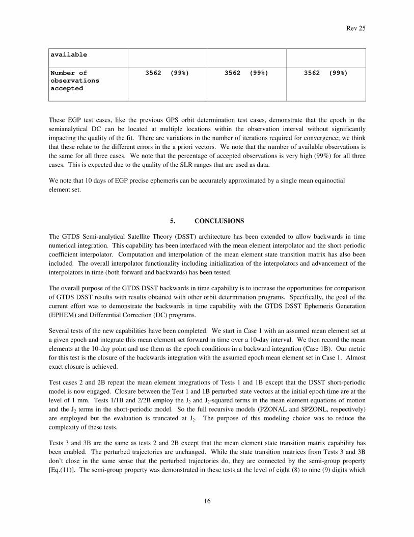
Among other things, these cases test GTDS operation with a large number of ground based sensors. Table 7. GTDS DSST Orbit Determination Test Cases for the EGP satellite (Test Table 7. GTDS DSST Orbit Determination Test Cases for the EGP satellite (Test Table 7. GTDS DSST Orbit Determination Test Cases for the EGP satellite (Test Table 7. GTDS DSST Orbit Determination Test Cases for the EGP satellite (Test Cases 13, 14, and 15)Cases 13, 14, and 15)Cases 13, 14, and 15)Cases 13, 14, and 15) Parameter Test Case 13 Test Case 14 Test Case 15

Epoch of the

solve-for vector

within the

observation span

Epoch at the

beginning of the

observation span

Epoch at the end

of the observation

span

Epoch at an

intermediate point

in the observation

span

Iterations to DC

convergence

7 5 5

Converged semi-

major axis

standard deviation

0.693 cm 0.432 cm 0.216 cm

Converged solar

radiation pressure

coefficient

0.14164574D+01 0.141610744D+01 0.142206157D+01

Converged solar

radiation pressure

coefficient

standard deviation

0.179D-01 0.179D-01 0.180D-01

Converged

atmosphere drag

parameter

0.4593108D+01 0.459162142D+01 0.4590957405D+01

Converged

atmosphere drag

parameter standard

deviation

0.613D-01 0.613D-01 0.613D-01

Converged position

error RMS, meters

7.7115502 7.7117070 7.7122563

Initial Weighted

RMS

13563.2 14.2 177.2

Converged Weighted

RMS

3.9244741 3.9246078 3.926902

Number of

observations

3580 3580 3580

Rev 25

16

available

Number of

observations

accepted

3562 (99%) 3562 (99%) 3562 (99%)

These EGP test cases, like the previous GPS orbit determination test cases, demonstrate that the epoch in the

semianalytical DC can be located at multiple locations within the observation interval without significantly

impacting the quality of the fit. There are variations in the number of iterations required for convergence; we think

that these relate to the different errors in the a priori vectors. We note that the number of available observations is

the same for all three cases. We note that the percentage of accepted observations is very high (99%) for all three

cases. This is expected due to the quality of the SLR ranges that are used as data.

We note that 10 days of EGP precise ephemeris can be accurately approximated by a single mean equinoctial

element set.

5. CONCLUSIONS

The GTDS Semi-analytical Satellite Theory (DSST) architecture has been extended to allow backwards in time

numerical integration. This capability has been interfaced with the mean element interpolator and the short-periodic

coefficient interpolator. Computation and interpolation of the mean element state transition matrix has also been

included. The overall interpolator functionality including initialization of the interpolators and advancement of the

interpolators in time (both forward and backwards) has been tested.

The overall purpose of the GTDS DSST backwards in time capability is to increase the opportunities for comparison

of GTDS DSST results with results obtained with other orbit determination programs. Specifically, the goal of the

current effort was to demonstrate the backwards in time capability with the GTDS DSST Ephemeris Generation

(EPHEM) and Differential Correction (DC) programs.

Several tests of the new capabilities have been completed. We start in Case 1 with an assumed mean element set at

a given epoch and integrate this mean element set forward in time over a 10-day interval. We then record the mean

elements at the 10-day point and use them as the epoch conditions in a backward integration (Case 1B). Our metric

for this test is the closure of the backwards integration with the assumed epoch mean element set in Case 1. Almost

exact closure is achieved.

Test cases 2 and 2B repeat the mean element integrations of Tests 1 and 1B except that the DSST short-periodic

model is now engaged. Closure between the Test 1 and 1B perturbed state vectors at the initial epoch time are at the

level of 1 mm. Tests 1/1B and 2/2B employ the J2 and J2-squared terms in the mean element equations of motion

and the J2 terms in the short-periodic model. So the full recursive models (PZONAL and SPZONL, respectively)

are employed but the evaluation is truncated at J2. The purpose of this modeling choice was to reduce the

complexity of these tests.

Tests 3 and 3B are the same as tests 2 and 2B except that the mean element state transition matrix capability has

been enabled. The perturbed trajectories are unchanged. While the state transition matrices from Tests 3 and 3B

don’t close in the same sense that the perturbed trajectories do, they are connected by the semi-group property

[Eq.(11)]. The semi-group property was demonstrated in these tests at the level of eight (8) to nine (9) digits which

Rev 25

17

was consistent the remainder of this process. Matlab was employed to achieve the matrix inversion required to

demonstrate the semi-group property.

The two differential correction cases (Test Cases 9, 10 and 11 for the GPS case and Test Cases 13, 14, and 15 for the

EGP case) provide further test of the backwards integration with time capability. Cases 9 and 13 are conventional

DSST DC runs with the solve-for epoch at the beginning of the observation span (2 days for the GPS case and 10

days for the EGP case). Cases 10 and 14 put the solve-for epoch at the end of the observation span. Thus the DSST

backwards integration capability is tested in the DC context with rather complete models for both the mean element

equations of motion and the short-periodic model. We note that these cases (10 and 14) also test the interaction

between the DSST backwards integration capability and several GTDS physical model binary files. Finally, Test

Cases 11 and 15 place the solve-for epoch at an intermediate point in the observation span requiring the integration

to go both backwards and forwards within a single DC iteration. It is satisfying that all three GPS cases and EGP

cases give similar results, respectively.

Another way to look at these tests is with respect to how they exercise the partial derivative capability:

• Test Cases 3 and 3B just compute the B2 matrix (see Eq. 7)

• Test Cases 9, 10, and 11 compute the B2 matrix and the B3 matrix (see Eq. 8). For the B3 matrix, only the

solar radiation pressure parameter partial derivatives are computed.

• Test Cases 13, 14, and 15 also compute the B2 and B3 matrices. Now the B3 matrix includes both the solar

radiation pressure and atmospheric drag parameter partial derivatives.

Both the GPS and EGP cases demonstrate that long arcs of observation data can be accurately compressed into a

single nonsingular mean element set. Sequences of nonsingular mean element sets are of interest for studies that try

to improve the prediction of the long term motion of such space objects.

Version control for the Linux GTDS R&D orbit computation program used in this study is maintained using the

subversion utility [21]. Finally we have given several GTDS DSST input files as examples.

6. FUTURE WORK

None of the test cases completed for this paper actually exercise the finite differencing method. The A matrix in Eq.

(9) is computed using just the closed-form J2 terms (see GTDS DSST subroutine J2PART). For the solar radiation

pressure and atmospheric drag parameter partial derivatives, the D matrix in Eq. (10) is just the portion of the mean

element rates due to respective perturbation divided by the parameter. See Eq. (2-94) in Green [2]. But several

finite differencing options are connected to the GTDS DSST keyword SSTAPGFL. These options should be tested

using the methods and cases developed in this paper. If the finite differencing approach causes observable error,

consideration should be given to analytical and quadrature approaches for reducing the dependence on finite

differences.

We would like to develop a test for the B3 matrices (parameter partials) that connects the values from the forward

integration with the values from the backward integration. This would be analogous to the semi-group property test

for the mean element state transition matrix.

The association of the DSST with the Runge-Kutta 4 integration stems from the initial build of the DSST in the

early 1980s. At that time, time intervals of just a few days were the primary interest. We would like to investigate

the application of Explicit Runge-Kutta Methods of Higher Order methods such as the Dorman & Prince 8(6) that is

described in [22] to the DSST orbit propagator.

Rev 25

18

We would like to undertake covariance propagation tests. One case would use the DSST DC to fit a set of

observations. The covariance would be recorded at the epoch. One can then use the DSST ephemeris program to

propagate that covariance forward to some time in the future and then backward to the original epoch again. The

covariance should be the same modulus any differences from numerical artifacts. The existing Extended

Semianalytical Kalman Filter (ESKF) [3, 4] may also play a role in these tests.

Another test that could be run with the DSST DC is a demonstration that when one moves the initial state epoch

from the beginning of the fitspan to the middle and then to the end of the fitspan that the covariance should be

minimal at the center of the fitspan. This should match the covariance when propagated with EPHEM from the

beginning to the end of the fitspan and from the end of the fitspan back to the beginning.

Finally, to demonstrate the value of the enhanced GTDS DSST functionality, we propose to develop a Spherical

Simplex Unscented Kalman Filter (SSUKF) based on the Spherical Simplex Unscented Transformation [23] to

estimate the mean equinoctial elements directly from the tracking data.

ACKNOWLEDGEMENT

Paul Cefola’s effort on this problem was supported by Pacific Defense Solutions. The authors acknowledge Zachary

Folcik’s (MIT LL) significant contribution to this effort. The contribution of several Draper Laboratory staff and

many MIT graduate students in the evolution of Linux GTDS R&D is gratefully acknowledged. The numerical

results described in this paper were generated on a multi-core PC with an Intel Core i7 960 Processor and an

NVIDIA GEFORCE GTX 580 graphical processor running the Linux Ubuntu 11.04 server distribution. This

machine was designed, assembled, and tested by MV Tech. Inc., Vineyard Haven, MA.

APPENDIX A – GPS Input File

CONTROL DC GPSSAT 0099999

EPOCH 1081109.0 001446.0000

ELEMENT1 10 1 1-1.36990181020000E+04-8.48585960000000E+03+2.14410746720000E+04

ELEMENT2 +9.77264236179275E-01-2.46212135521801E+00-3.53083683724679E-01

OBSINPUT 20 1081109001446.0000 1081111001446.0000

ORBTYPE 5 1 11 43200.0000 1.0

DMOPT

OBSDEV 21 22 23 10.0 10.0 10.0

END

DCOPT

CONVERG 30 3 0.0001

EDIT 3 3.0

PRINTOUT 1 4 10.0

END

OGOPT

POTFIELD 1 11

SSTESTFL 1 2 0 0.0

SSTAPGFL 1 0 0 0.0 0.0 1.0

SPGRVFRC 1 1 1 2.0 1.0 1.0

SPTESSLC 6 6 4 2.0 -8.0 8.0

SPNUMGRV 7 1 10 2.0 2.0 3600.0

SPZONALS 8 5 11

SPJ2MDLY 4 4 5 2.0 SPMDAILY 8 8 5

POLAR 1 1.0

MAXDEGEQ 1 16.0

MAXORDEQ 1 16.0

SOLRAD 1 1.0

SOLRDPAR 1

Rev 25

19

NCBODY 1 2 3

SCPARAM +1.00000000000000E-06+1.00000000000000E+02

STATEPAR 3 1

STATETAB 1 2 3 4.0 5.0 6.0

END

FIN

APPENDIX B – EGP Input File CONTROL DC SATSAT-0 0016908

EPOCH 1020829.0 215305.292

ELEMENT1 1 6 1 7866.628863685799 1.51219480042467E-03 49.99690802918278

ELEMENT2 0 234.0990114753167 44.20804018942176 315.9207248379734

OBSINPUT 5 1020829215305.292 1020908215305.292

ORBTYPE 5 1 11 43200.0 1.0

DMOPT

/L75L 1 0999 3 75.8889 0505202.5723 0002010.0469

/L79L 1 0999 3 804.5133 -351858.1309 1490035.5633

/L11L 1 0999 3 1839.4914 0325330.2604 2433438.3848

/L23L 1 0999 3 274.7100 0434725.8481 1252636.4466

/L68L 1 0999 3 760.5880 0245437.9659 0462401.3133

/L73L 1 0999 3 102.1025 0333439.6990 1355613.3396

/L66L 1 0999 3 98.7288 0362754.9151 3534740.8834

/L74L 1 0999 3 539.8719 0470401.6902 0152936.0992

/L06L 1 0999 3 241.8078 -290247.3956 1152048.2860 /L04L 1 0999 3 2004.7519 0304048.9635 2555905.2899

/L72L 1 0999 3 28.3126 0310551.1457 1211130.2640

/L94L 1 0999 3 31.8214 0565654.7843 0240332.6660

/L62L 1 0999 3 74.5050 0601301.7555 0242340.3816

/L38L 1 0999 3 1407.2622 -255322.9546 0274110.2274

/L09L 1 0999 3 19.6660 0390114.1792 2831020.3022

/L93L 1 0999 3 665.8497 0490839.9041 0125240.8289

/L36L 1 0999 3 2489.3114 -162756.5816 2883025.3609

/L20L 1 0999 3 3067.9800 0204225.9865 2034438.7206

/L26L 1 0999 3 82.1399 0393624.9678 1155331.3934

/L70L 1 0999 3 1323.3081 0434516.8903 0065516.0429

/L63L 1 0999 3 951.8148 0465238.0256 0072754.7913

END

DCOPT

CONVERG 30 3 1 0.0001

EDIT 3 3.0

BATCHTYP 7

TRACKELV 3 1.0

TRACKELV 13 3.0

/L75L 001 2

/L79L 001 2

/L11L 001 2

/L23L 001 2

/L68L 001 2

/L73L 001 2

/L66L 001 2

/L74L 001 2

/L06L 001 2

/L04L 001 2

/L72L 001 2

/L94L 001 2

/L62L 001 2

/L38L 001 2

/L09L 001 2

/L93L 001 2

/L36L 001 2

/L20L 001 2

Rev 25

20

/L26L 001 2

/L70L 001 2

/L63L 001 2

PRINTOUT 1 4 10.0

ELLMODEL 1 6378.13655 298.256421867

END

OGOPT

DRAG 1 1.0

ATMOSDEN 1

DRAGPAR 2 2.0 1.0

DRAGPAR2 1 1

POTFIELD 1 11

STATEPAR 3 1

STATETAB 1 2 3 4.0 5.0 6.0

SETIDE 1 0.29D0

SOLRAD 1 1.0

SOLRDPAR 2 1.2 0.005

POLAR 1 1.0

SPGRVFRC 1 1 1 1.0 1.0 1.0

SSTESTFL 1 2 0 0.0 SSTAPGFL 1 0 0 1.0 6.0 1.0

SPTESSLC 14 14 4 2.0 -10.0 10.0

SPZONALS 8 7 16

SPMDAILY 14 14 12

SPJ2MDLY 8 8 6 1.0

AVRDRAG 5 3 3

RESONPRD 259200.0

MAXDEGEQ 1 30.0

MAXORDEQ 1 30.0

NCBODY 1 2 3

SCPARAM +3.14150000000000E-06+6.85000000000000E+02

END

FIN

REFERENCES

1. P. J. Cefola, D. Phillion, and K. S. Kim, Improving Access to the Semi-Analytical Satellite Theory, pre-print

AAS 09-341, presented at the AAS/AIAA Astrodynamic Specialist Conference, Pittsburg, PA, August 2009.

2. Andrew Joseph Green, Orbit Determination and Prediction Processes for Low Altitude Satellites, Ph.D

Thesis, Department of Aeronautics and Astronautics, MIT, December 1979 (CSDL-T- 703).

3. Stephen Paul Taylor, Semi-analytical Satellite Theory and Sequential Estimation, Master of Science Thesis,

Department of Mechanical Engineering, MIT, September 1981 (CSDL-T- 757).

4. Elaine Ann Wagner, Application of the Extended Semianalytical Kalman Filter to Synchronous Orbits,

Master of Science Thesis, Department of Aeronautics and Astronautics, MIT, June 1983 (CSDL-T- 801)

5. Robert Lawrence Herklotz, Incorporation of Cross-Link Range Measurements in the Orbit Determination

Process to Increase Satellite Constellation Autonomy, Ph.D. Thesis, Department of Aeronautics and

Astronautics, MIT, December 1987 (CSDL-T- 964).

6. Gerald J. Bierman, Factorization Methods for Discrete Sequential Estimation, Academic Press: New York,

1977.

7. Folcik, Z. J., Orbit Determination Using Modern Filters/Smoothers and Continuous Thrust Modeling, M.S.

Thesis. Department of Aeronautics and Astronautics, MIT, 2008

Rev 25

21

8. C. Sabol, T. Sukut, K. Hill, K. T. Alfriend, B. Wright, Y. Li, and P. Schumacher, Linearized Orbit Covariance

Generation and Propagation Analysis Via Simple Monte Carlo Simulations, AAS 10-134, presented at the

AAS/AIAA Spaceflight Mechanics Meeting, San Diego, CA, 11-15 February 1996.

9. Fonte, D., Implementing a 50 x 50 Gravity Field Model in an Orbit Determination System, M.S. Thesis.

Department of Aeronautics and Astronautics, MIT, 1993.

10. Carter, S., Precision Orbit Determination From GPSR Navigation Solutions, M.S. Thesis. Department of

Aeronautics and Astronautics, MIT, 1996.

11. Fischer, J., The Evolution of Highly Eccentric Orbits, M.S. Thesis. Department of Aeronautics and

Astronautics, MIT, 1998.

12. Granholm, G., Near-Real Time Atmosphere Density Correction Using Space Catalog Data, M.S. Thesis.

Department of Aeronautics and Astronautics, MIT, 2000.

13. Bergstrom, S. E., An Algorithm for Reducing Atmospheric Density Model Errors Using Satellite Observation

Data in Real-Time, M.S. Thesis. Department of Aeronautics and Astronautics, MIT, 2002.

14. Lyon, R. H., Geosynchronous Orbit Determination Using Space Surveillance Network Observations And

Improved Radiative Force Modeling, M.S. Thesis. Department of Aeronautics and Astronautics, MIT, 2004.

15. M. Slutsky, "Zonal Harmonic Short-Periodic Model Developed for the Precision Orbit Propagation

Contract," Charles Stark Draper Laboratory, Internal Memorandum PL-016-81-MS, 30 November 1981.

16. NGA GPS Satellite (Center of Mass) Precise Ephemeris Page, http://earth-

info.nga.mil/GandG/sathtml/PEexe.html , accessed 8 September 2011

17. NGA GPS Ephemeris/Station/Antenna Offset Documentation, http://earth-

info.nga.mil/GandG/sathtml/gpsdoc2011_07a.html, accessed 8 September 2011

18. Degnan, J. J., The History and Future of Satellite Laser Ranging, vu-graph presentation accessed at

http://ilrs.gsfc.nasa.gov/docs/degnan_0603.pdf, 8 September 2011

19. Long, A. C., and L. W. Early, System Description and User’s Guide for the GTDS R&D Averaged Orbit

Generator, Computer Sciences Corporation, CSC/SD-78/6020, November 1978 (electronic copy with new

preface generated in 2010).

20. P. Cefola, R&D GTDS Semianalytical Satellite Theory Input Processor, Charles Stark Draper Laboratory,

Internal Memorandum ESD-92-582/SGI GTDS-92-001, rev 1, February 8, 1993 (electronic copy available).

21. Pilato, C. Michael, B. Collins-Sussman, and Brian W. Fitzpatrick, Version Control with Subversion, O’Relly

Media Inc, 2004.

22. Ernst Hairer, Syvert P. Norsett, and Gerhard Wanner, Solving Ordinary Differential Equations I – Nonstiff

Problems, 2nd

Revised Edition, Springer, 2009.

23. Julier, S. J., “The Spherical Simplex Unscented Transformation”, Proceedings of the American Control

Conference, Denver, Colorado, June 2003, pp. 2430-2434.

demonstration of the dsst state transition matrix

Documents