A density curve is the graph of a continuous probability distribution. It must satisfy the following properties:

Density Curve

1. The total area under the curve must equal 1.

2. Every point on the curve must have a vertical height that is 0 or greater. (That is, the curve cannot fall below the x-axis.)

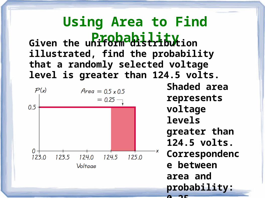
Using Area to Find Probability

Given the uniform distribution illustrated, find the probability that a randomly selected voltage level is greater than 124.5 volts.

Shaded area represents voltage levels greater than 124.5 volts. Correspondence between area and probability: 0.25.

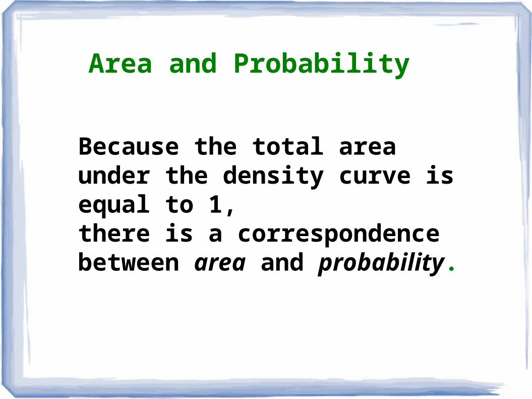
Because the total area under the density curve is equal to 1, there is a correspondence between area and probability.

Area and Probability

Relative Frequency Histogram

Relative frequency =Frequency / Data size

Bandwidth of class

It includes the same class limits as a frequency distribution, but the frequency of a class is replaced with a relative frequencies. So that the area represents the proportion of data between the interval of your choice.

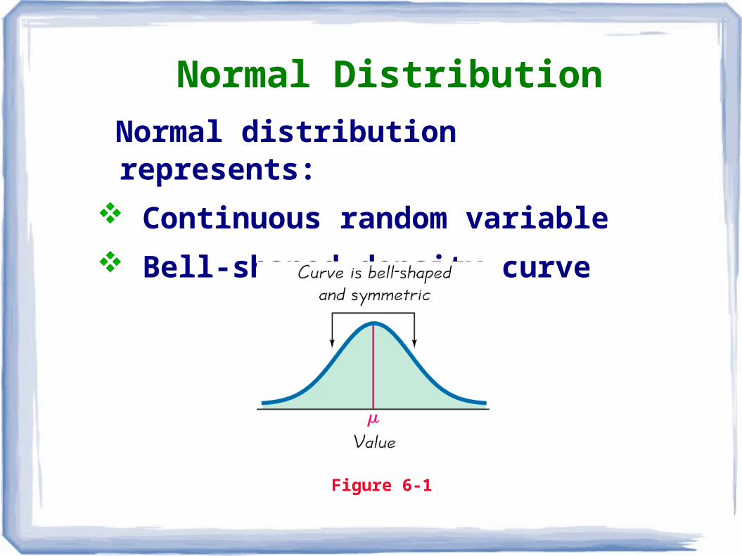
Normal distribution represents:

Continuous random variable

Bell-shaped density curve

Normal Distribution

Figure 6-1

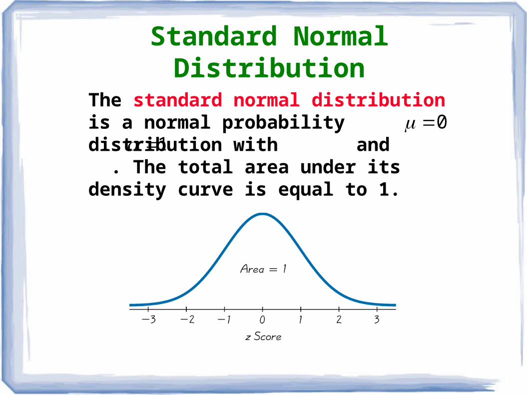
Standard Normal Distribution

The standard normal distribution is a normal probability distribution with and . The total area under its density curve is equal to 1.

0 1

The probability of standard normal distribution less than 1.27 is 0.8980.

Example – Normal Table

( 1.27) 0.8980P z

Look at Normal Table

If one value is randomly selected from the standard normal distribution, find the probability that it shows above –1.23.

Probability of randomly selecting a value above –1.23 is 0.8907.

Example (2)

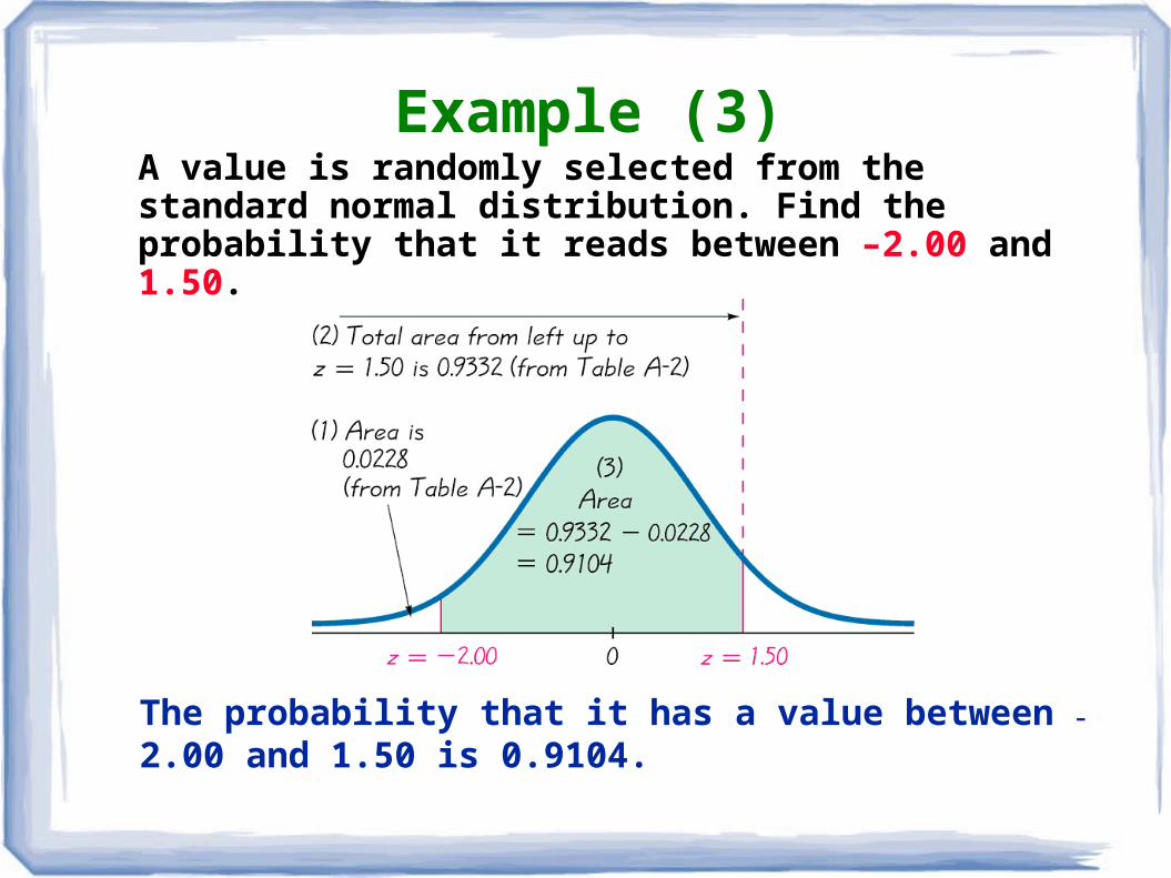
A value is randomly selected from the standard normal distribution. Find the probability that it reads between –2.00 and 1.50.

The probability that it has a value between – 2.00 and 1.50 is 0.9104.

Example (3)

Standardization

Round z scores to 2 decimal places

Given the mean (mu) and the standard deviation (sigma) we can convert the value x into the Z score.

X

Z

Converting to a Standard Normal Distribution

X

Z

Example

z = 174 – 172

29 = 0.07

SD =29 Mean = 172

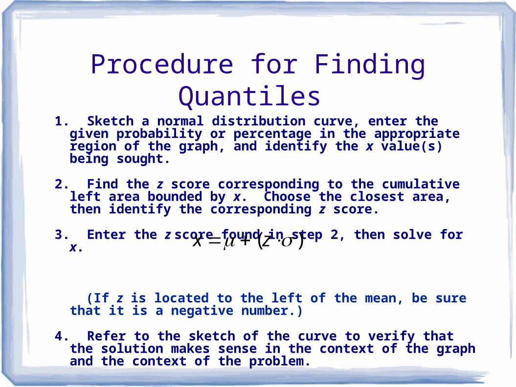
1. Sketch a normal distribution curve, enter the given probability or percentage in the appropriate region of the graph, and identify the x value(s) being sought.

2. Find the z score corresponding to the cumulative left area bounded by x. Choose the closest area, then identify the corresponding z score.

3. Enter the z score found in step 2, then solve for x.

(If z is located to the left of the mean, be sure that it is a negative number.)

4. Refer to the sketch of the curve to verify that the solution makes sense in the context of the graph and the context of the problem.

Procedure for Finding Quantiles

( )x z

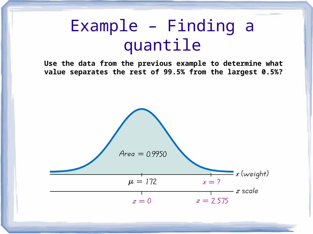
Example – Finding a quantile

Use the data from the previous example to determine what value separates the rest of 99.5% from the largest 0.5%?

x = 172 + (2.575)(29)x = 246.675 (247 rounded)

Example – Finding a quantile

Sample Mean

The sampling distribution of the mean is the distribution of sample means, with all samples having the same sample size n taken from the same population. (The sampling distribution of the mean is typically represented as a probability distribution.)

xx

n

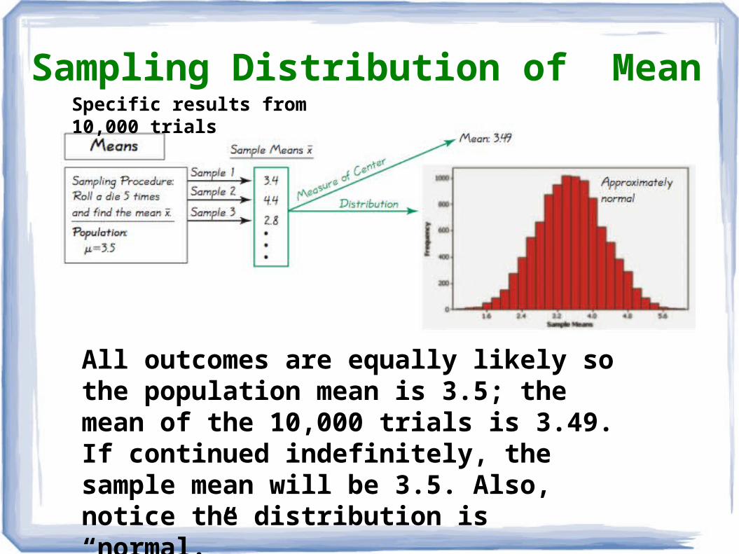
Sampling Distribution of Mean

All outcomes are equally likely so the population mean is 3.5; the mean of the 10,000 trials is 3.49. If continued indefinitely, the sample mean will be 3.5. Also, notice the distribution is “normal.”

Specific results from 10,000 trials

Central Limit Theorem

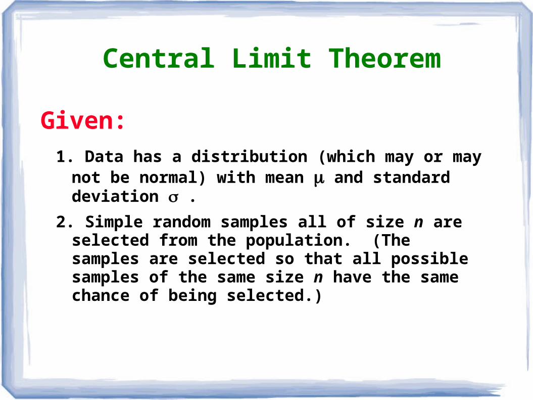
1. Data has a distribution (which may or may not be normal) with mean and standard deviation .

2. Simple random samples all of size n are selected from the population. (The samples are selected so that all possible samples of the same size n have the same chance of being selected.)

Given:

1. The distribution of sample mean will, as the sample size increases, approach a normal distribution.

2. The mean of the sample means is the population mean .

3. The standard deviation of all sample means

is

Conclusions:

Central Limit Theorem – cont.

n.

Practical Rules Commonly Used

1. For samples of size n larger than 30, the distribution of the sample means can be approximated reasonably well by a normal distribution. The approximation gets closer to a normal distribution as the sample size n becomes larger.

2. If the original population is normally distributed, then for any sample size n, the sample means will be normally distributed (not just the values of n larger than 30).

Assume the population of weights of men is normally distributed with a mean of 172 lb and a standard deviation of 29 lb.

Example

a) Find the probability that if an individual man is randomly selected, his weight is greater than 175 lb.

b) Find the probability that 20 randomly selected men will have a mean weight that is greater than 175 lb (so that their total weight exceeds the safe capacity of 3500 pounds).

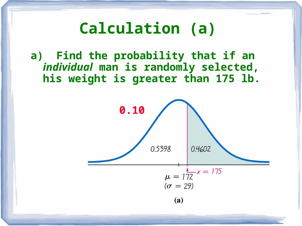
a) Find the probability that if an individual man is randomly selected, his weight is greater than 175 lb.

Calculation (a)

175 1720.10

29z

0.10

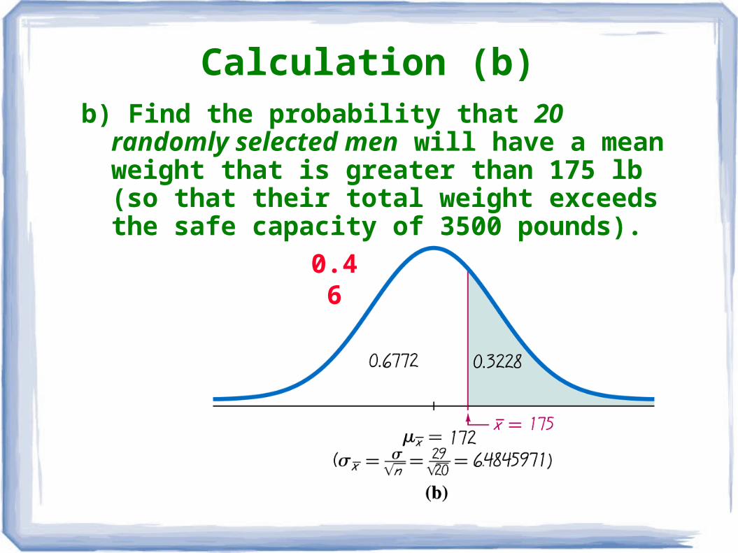
b) Find the probability that 20 randomly selected men will have a mean weight that is greater than 175 lb (so that their total weight exceeds the safe capacity of 3500 pounds).

Calculation (b)

175 1720.46

29

20

z

0.46

QQ plot

A quantile-quantile plot (or normal quantile plot) is a graph of points (x,y), where each x value is from the original set of sample data, and each y value is the corresponding z score that is a quantile value expected from the standard normal distribution.

Example

Normal: Histogram of IQ scores is close to being bell-shaped, suggests that the IQ scores are from a normal distribution. The QQ plot shows points that are reasonably close to a straight-line pattern. It is safe to assume that these IQ scores are from a normally distributed population.

Determining Whether It To Assume that Sample Data are From a

Normally Distributed Population1. Histogram: Construct a histogram. Reject

normality if the histogram departs dramatically from a bell shape.

2. Outliers: Identify outliers. Reject normality if there is more than few outliers present in one side.

3. QQ Plot: If the histogram is basically symmetric and there are only few outliers, use technology to generate a QQ plot.

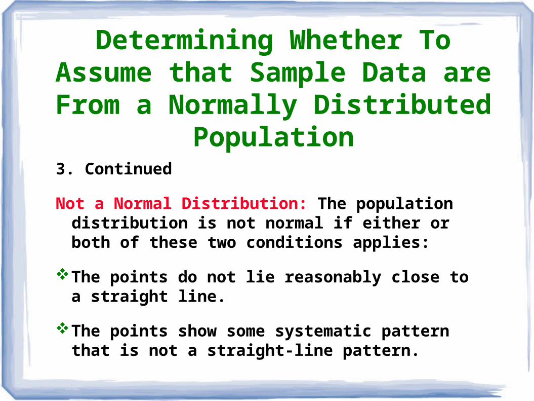
Determining Whether To Assume that Sample Data are From a

Normally Distributed Population

3. Continued

Use the following criteria to determine whether or not the distribution is normal.

Normal Distribution: The population distribution is normal if the pattern of the points is reasonably close to a straight line and the points do not show some systematic pattern that is not a straight-line pattern.

Determining Whether To Assume that Sample Data are From a

Normally Distributed Population

3. Continued

Not a Normal Distribution: The population distribution is not normal if either or both of these two conditions applies:

The points do not lie reasonably close to a straight line.

The points show some systematic pattern that is not a straight-line pattern.

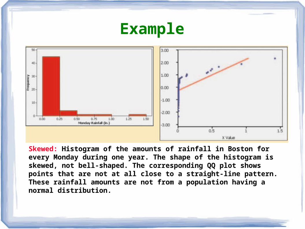
Example

Skewed: Histogram of the amounts of rainfall in Boston for every Monday during one year. The shape of the histogram is skewed, not bell-shaped. The corresponding QQ plot shows points that are not at all close to a straight-line pattern. These rainfall amounts are not from a population having a normal distribution.

Example

Uniform: Histogram of data having a uniform distribution. The corresponding QQ plot suggests that the points are not normally distributed because the points show a systematic pattern that is not a straight-line pattern. These sample values are not from a population having a normal distribution.