department of mathematics saarland university saarbruc ... · first order variational methods this...
TRANSCRIPT

Higher Order Variational Methods for Noise Removal inSignals and Images
Diploma Thesis
Stephan Didas
under supervision of
Prof. Joachim Weickert
Department of MathematicsSaarland University
Saarbrucken, April 2004– Corrected version, October 2004 –

Preface
Variational methods have become more and more important in image processingduring the last years. They offer an intuitive way to understand the noise removaland image restoration process as minimisation of an energy functional. This energyfunctional provides the opportunity to compare the quality of two filtered versionsof the same input image and thus can be seen as a quality measure.
Variational image restoration methods in general yield high quality results. Non-linear approaches are known to suffer from the effect of turning smooth grey valuechanges in piecewise constant regions. This effect is called stair-casing.
One can interpret stair-casing as the result of energy functionals that rewardpiecewise vanishing first derivatives which yields piecewise constant signals and im-ages. A way to circumvent this would be to use higher derivatives in the penaliserterms: Piecewise vanishing second derivatives would lead to piecewise linear re-sults that could better fit to smooth grey value changes. Higher derivatives couldanalogously yield piecewise polynomials of higher degree.
There is a growing interest in higher order variational methods in the literature.Nielsen, Florack and Deriche (see [18]) have studied linear energy functionals ofarbitrary order. They derive basic scale-space properties and give efficient filteringalgorithms for the linear case. Greer and Bertozzi further investigate some theoret-ical properties of special fourth order evolution equations used in image restoration(see [10]). Other authors rather concentrate on the goal of showing the use ofhigher order methods for practical purposes. Chan, Marquina and Mulet (see [5])study nonlinear energy functionals of second order and the related diffusion filter-ing with derivative orders up to four. Total variation methods with the secondderivative leading to fourth order partial differential equations are used in [17] byLysaker, Lundervold and Tai. Besides images they consider one-dimensional signalprocessing. You and Kaveh [34] also use fourth order PDEs for filtering. Numericalexamples are presented which show that higher order methods can in practise beuseful for image denoising.
The goal of the present thesis is to investigate some theoretical and practicalaspects of higher order variational methods. We use different penaliser functionsand compare them in practical applications. To introduce variational methods somefacts about first order methods are summarised in Chapter 1.
In Chapter 2 we start with a continuous higher order energy functional anddeduce necessary and sufficient conditions for a function to be a minimiser of thisfunctional. The main result are the so-called Euler-Lagrange equations in one andtwo dimensions. A closer look is also taken at the natural boundary conditionswhich come with this partial differential equation if we impose no boundary condi-tions at our set of possible solutions. In the first order context the natural boundaryconditions are of Neumann type. This coincides with the usage of Neumann bound-ary conditions in image processing since they usually yield good visual results. Wewill see that for higher order functionals the boundary conditions may be a bitmore complicated. Signal processing results show that both natural and Neumannboundary conditions may lead to acceptable results, while in image processing Neu-mann boundary conditions are preferred. With the trace, the Frobenius norm, andthe determinant of the Hessian, equivalents for the second derivative in 2D energyfunctionals are discussed.
Chapter 3 discusses several approaches how to deduce continuous filtering meth-ods from energy functionals or corresponding Euler-Lagrange equations. In the caseof linear penalisers one can give direct minimisation methods in the Fourier domainas investigated in [18]. These methods are not applicable in the nonlinear context.Thus one considers the Euler-Lagrange equation and the corresponding diffusion
3

equations. Generalised higher order linear diffusion leads to convolution kernelsaxiomatically derived in [16]. We try to give an explanation for the behaviour ofsimple nonlinear filters in terms of forward and backward diffusion.
To use the methods presented in Chapter 3 in practice we need to discretisethem. With finite differences and spectral methods, two different ways for derivativeapproximation are presented in Chapter 4. We are especially interested in matrixrepresentations for discretisations. For finite differences we discuss possibilities toimplement both natural and Neumann boundary conditions.
With these discretisation matrices we give discrete versions of the minimisa-tion approaches in Chapter 5. We see that one can either start with a continuousenergy functional and discretise the corresponding Euler-Lagrange equations or dis-cretise the energy functional itself. Discretisations for nonlinear diffusion equationsobtained from the Euler-Lagrange equations are also investigated. A key pointare stability criterions for explicit methods we use to obtain most of the numeri-cal results presented in Chapter 6. These should give a visual impression of thepossibilities of nonlinear higher order filtering.
The last Chapter 7 concludes the thesis with a short summary including inter-esting questions arising in the thesis that invite to be further investigated.
At this place I would like to take the opportunity to thank the people thatmade this thesis possible. First I like to thank Prof. Joachim Weickert for theinteresting topic and for his constant support. Besides many theoretical conceptionshe provided me with an implementation of 2D higher order linear filtering withspectral methods. I also thank the members of the Mathematical Image AnalysisGroup at Saarland University – especially Dr. Bernhard Burgeth – for many hintsand discussions on image processing including higher order methods. I thank NatalieMarx – not only for her help on the correction of this thesis. My thank goes to mybrother Michael for arousing my interest in mathematical questions. In particular Iwould like to thank my parents for their permanent support that made my studiespossible.
4
Contents
1 First Order Variational Methods 7
2 Continuous Energy Functionals 112.1 The One-Dimensional Case . . . . . . . . . . . . . . . . . . . . . . . 13
2.1.1 The Problem . . . . . . . . . . . . . . . . . . . . . . . . . . . 132.1.2 The Euler-Lagrange Equation . . . . . . . . . . . . . . . . . . 132.1.3 Natural Boundary Conditions . . . . . . . . . . . . . . . . . . 152.1.4 Sufficient Conditions . . . . . . . . . . . . . . . . . . . . . . . 162.1.5 Applications . . . . . . . . . . . . . . . . . . . . . . . . . . . 17
2.2 The Two-Dimensional Case . . . . . . . . . . . . . . . . . . . . . . . 182.2.1 The Problem . . . . . . . . . . . . . . . . . . . . . . . . . . . 182.2.2 The Euler-Lagrange Equation . . . . . . . . . . . . . . . . . . 192.2.3 Natural Boundary Conditions . . . . . . . . . . . . . . . . . . 202.2.4 Sufficient Conditions . . . . . . . . . . . . . . . . . . . . . . . 222.2.5 Applications . . . . . . . . . . . . . . . . . . . . . . . . . . . 22
3 Continuous Filtering 293.1 Filtering Approaches . . . . . . . . . . . . . . . . . . . . . . . . . . . 29
3.1.1 Direct Minimisation of the Energy Functional . . . . . . . . . 293.1.2 Parabolic Differential Equations . . . . . . . . . . . . . . . . 313.1.3 Generalised Linear Diffusion . . . . . . . . . . . . . . . . . . . 32
3.2 Nonlinear Diffusion of Second Order . . . . . . . . . . . . . . . . . . 373.3 Application to Penalty Functions . . . . . . . . . . . . . . . . . . . . 38
3.3.1 Linear Filtering . . . . . . . . . . . . . . . . . . . . . . . . . . 383.3.2 Charbonnier . . . . . . . . . . . . . . . . . . . . . . . . . . . 393.3.3 Perona-Malik . . . . . . . . . . . . . . . . . . . . . . . . . . . 393.3.4 Total Variation Approximations . . . . . . . . . . . . . . . . 403.3.5 Total Variation . . . . . . . . . . . . . . . . . . . . . . . . . . 41
4 Discretisation 434.1 General Remarks and Notations . . . . . . . . . . . . . . . . . . . . 434.2 Finite Differences . . . . . . . . . . . . . . . . . . . . . . . . . . . . . 45
4.2.1 Matrix Notation . . . . . . . . . . . . . . . . . . . . . . . . . 494.2.2 Finite Differences and Polynomial Data Fitting . . . . . . . . 524.2.3 Neumann Boundary Conditions . . . . . . . . . . . . . . . . . 534.2.4 The Two-Dimensional Case . . . . . . . . . . . . . . . . . . . 54
4.3 Spectral Methods . . . . . . . . . . . . . . . . . . . . . . . . . . . . . 564.3.1 Matrix Notation . . . . . . . . . . . . . . . . . . . . . . . . . 574.3.2 Problems . . . . . . . . . . . . . . . . . . . . . . . . . . . . . 594.3.3 Higher Dimensions . . . . . . . . . . . . . . . . . . . . . . . . 62
5

5 Discrete Filtering 655.1 Discrete Energy Functionals . . . . . . . . . . . . . . . . . . . . . . . 655.2 Discretisation of the Euler-Lagrange Equation . . . . . . . . . . . . . 685.3 Methods with Parabolic Equations . . . . . . . . . . . . . . . . . . . 69
5.3.1 The Semi-Discrete Case . . . . . . . . . . . . . . . . . . . . . 695.3.2 The Discrete Case . . . . . . . . . . . . . . . . . . . . . . . . 72
6 Experimental Results 796.1 Filtering Results . . . . . . . . . . . . . . . . . . . . . . . . . . . . . 79
6.1.1 Filtering in 1D . . . . . . . . . . . . . . . . . . . . . . . . . . 806.1.2 Special Case: TV Approximation . . . . . . . . . . . . . . . . 816.1.3 Different Penalisers in 2D . . . . . . . . . . . . . . . . . . . . 87
6.2 Different Discretisation Methods . . . . . . . . . . . . . . . . . . . . 906.3 Combinations of Different Orders . . . . . . . . . . . . . . . . . . . . 92
7 Summary and Outlook 95
6

Chapter 1
First Order VariationalMethods
This chapter gives a short overview of first order variational methods in signaland image processing. First we mention how the notions signal and image areused during this thesis: In a continuous framework a signal is usually a real-valuedfunction f : Ω −→ R with Ω ⊆ R open. For our purposes it is normally sufficientto assume that Ω is an open interval. Sometimes we use Ω = R in considerationsin the continuous setting and then usually assume that f has compact support. Animage is also a real-valued function where Ω ⊆ R2 is an open two-dimensional set.We sometimes use the notion image as generic term including also signals. We oftendenote the initial image of a filtering or restoration process with f and the filteredversion with u.
Variational methods in image processing usually start with an energy functionalof the form
E(u) =∫Ω
((u− f)2 + α ϕ
(u2
x
))dx (1.1)
for one-dimensional examples or
E(u) =∫Ω
((u− f)2 + α ϕ
(|∇u|2
))dx (1.2)
in two dimensions. These methods are also called regularisation. The typicalenergy functionals consist of two terms:
1. The data term (also called similarity term) (u− f)2: This term rewardssimilarity to the initial image.
2. The smoothness term (also called regulariser or penaliser) ϕ(u2
x
): This
term rewards some kind of smoothness by involving the first derivative of theimage u. Different examples for the penaliser function ϕ are discussed below.
During this thesis we classify the methods with respect to the derivative orderthat appears in the smoothness term of the energy functional. Thus the methodsconsidered in this chapter are first order methods. The parameter α > 0 is calledregularisation parameter and serves as a weight between similarity to the initialdata and smoothness.
Variational methods in the above form can be related to (in general nonlinear)diffusion filtering. A detailed investigation of this relation is presented in [22]. With
7

8 CHAPTER 1. FIRST ORDER VARIATIONAL METHODS
an additional artificial time variable for u and the assumption that the initial imageis u(·, 0) = f we get the diffusion equation
ut =d
dx
(ϕ′(u2
x
)ux
)(1.3)
for the functional (1.1). In two dimensions the corresponding diffusion equationreads as
ut = div(ϕ′(|∇u|2
)∇u)
with initial condition u(·, 0) = f . In both cases Neumann boundary conditions
∂nu = 0 for all x ∈ ∂Ω
are assumed. We will further explain how to obtain this relation in Chapter 3. Wenote that the regulariser ϕ(x2) corresponds to the diffusivity ϕ′(x2). We should alsomention that first order variational methods lead to diffusion equation with highestderivative order two.
The first example of variational methods in literature can be found in a paper byTikhonov (see [28]). Here the general regularisation method with linear penaliser
ϕ(x) = x
is proposed in the context of giving approximative solutions to ill-posed problems.First applications in the field of image processing are presented in [3] and [19].There are different classical penaliser functions used for image processing.
Besides the Tikhonov regulariser we also consider the function
ϕ(x) = 2λ2
(√1 +
x
λ2− 1)
for λ > 0
which was first suggested by Charbonnier et al. (see [6]) in 1994.Rudin, Osher and Fatemi (see [21]) proposed regularisation approaches based
on minimisation of the total variation∫Ω
|∇u|dx
of u. To stay in the framework sketched above one can approximate total variationbased filtering with the penaliser family
ϕ(x) = 2√
ε2 + x− 2ε for ε > 0.
These functions are C∞ and for ε −→ 0 they approximate the absolute value of theargument x. These approximations are discussed by Acar and Vogel in [1].
Perona and Malik suggested another penaliser in the context of nonlinear diffu-sion equations (see [20]) which reads as
ϕ(x) = λ2 ln(1 +
x
λ2
)for λ > 0.
Usually several assumptions on the penaliser are made:
1. ϕ is differentiable and increasing (ϕ′ > 0).
2. ϕ(x2) is convex in x. This is used to prove the existence of a minimiser. Wenote that this assumption is not satisfied for the Perona-Malik penaliser.
3. There are constants c1, c2 > 0 such that c1x2 < ϕ(x2) < c2x
2 for all x2.

9
Under these assumptions some scale-space properties for regularisation methodscan be shown: Schnorr (see [23]) has deduced well-posedness and regularity ofthe solution, average grey value invariance and the minimum-maximum principle.Scherzer and Weickert (see [22]) have further shown the Lyapunov property andconvergence to the average grey value for α −→ ∞. These scale-space propertiesare very similar to the properties of nonlinear diffusion filtering as presented in [31].
One should mention that contrast enhancement is only possible for nonconvexregularisers. In the diffusion filter framework one can motivate this with investiga-tions of forward-backward diffusion:
Let us consider the one-dimensional nonlinear diffusion equation
ut =d
dx
(ϕ′(u2
x
)ux
).
We then are interested in the flux function
Φ(ux) = ϕ′(u2
x
)ux
which allows us to rewrite the diffusion equation to
ut = Φ′(ux)uxx.
If Φ′(ux) > 0 within a region the nonlinear diffusion equation behaves like a scaledversion of ut = uxx. In this regions the equation is well-posed, and we call thebehaviour forward diffusion. In regions where Φ′(ux) < 0 the equation behaveslike a scaled version of the ill-posed equation ut = −uxx. This so-called backwarddiffusion acts edge-enhancing.
We should note that among the penalisers presented above only the Perona-Malik penaliser allows backward diffusion. This can be an advantage in terms ofedge-enhancement though it introduces some degree of ill-posedness. More infor-mation on this remarks can be found in [31], for example. In Chapter 3 we willcarry over these considerations to second order filtering.
Backward diffusion is useful to enhance blurred edges. In regions with smoothgrey value changes however it can reduce the quality of an image leading to thestair-casing effect.
We have shortly introduced first order variational methods. In the next chapterwe start to carry over some essential parts of this theory to the higher order case.

10 CHAPTER 1. FIRST ORDER VARIATIONAL METHODS

Chapter 2
Continuous EnergyFunctionals
Variational methods for noise removal are based on the notion of minimisation ofenergy functionals. We imagine that unwanted features of an image (such as noise)result in high energy values. In this chapter we start with an energy functional
E(u) =∫Ω
E (z, u(z), Du(z), . . . , Dmu(z)) dz (2.1)
and search for necessary and sufficient conditions for a function to be optimal withrespect to this energy functional. We assume that Ω ⊂ Rn is open and E is anintegrable real-valued function.
First we summarise some results of calculus that are needed throughout thischapter and explain the basic procedure. For the treatment of the energy functionalswe need some statements about parameter depending integrals and exchanging theorder of integration and differentiation. We cite the following lemma from [30]:
Lemma 2.1 (Parameter Depending Integrals) Let n, m ∈ N \ 0, B ⊂ Rn
compact with boundary of measure 0, and C ⊂ Rm. Consider integrals of the form
F (y) =∫B
f(x, y)g(x)dx
depending on the parameter y ∈ C. If C is open and if f and ∂f∂yj
are continuous inB×C then ∂F
∂yjis continuous and one can exchange integration and differentiation:
∂F
∂yj(y) =
∫B
∂f
∂yj(x, y)g(x)dx.
Even if we integrate formally over an unbounded set we deal with signals and imageswhich typically have a bounded support. We usually have an interval or a rectangleas integration domain B.
The following lemma will allow us to write the necessary condition for a min-imiser as a partial differential equation.
Lemma 2.2 (Fundamental Lemma of the Calculus of Variations)Let f be a contiuous, real-valued function on some open set Ω ⊂ Rn, and supposethat ∫
Ω
f(x)η(x)dx = 0 for all η ∈ C∞C (Ω)
11

12 CHAPTER 2. CONTINUOUS ENERGY FUNCTIONALS
holds. Then we havef(x) = 0 for all x ∈ Ω.
Remark 2.3 Variants of this lemma with different proofs can be found in [9], [2],and [8]. Usually the lemma is proven by contradiction. The proof is primarly basedon the fact that for continuous f a single nonzero point leads to an open set wherethe absolute value of f is greater than some positive bound. Then the space C∞
C
is rich enough to contain a suitable function η which also has positive values in theopen set, and the integral is not zero. The main difference between the differentproofs cited above is the actual choice for η.
To reach the minimum of E we study the behaviour of E if we disturb theargument function u. Let η ∈ Cm([a, b]). Then we consider the function Ψ :(−ε0, ε0) −→ R defined by
Ψ(ε) := E(u + εη). (2.2)
This function describes the growth of E in direction η. Ψ′(0) can be considered asdirectional derivative of E in direction η: It describes the change of E at the pointu in direction η.
Definition 2.4 (Variation) We define the first variation of E at the point uin direction η as
δE(u, η) := Ψ′(0). (2.3)
Higher variations are defined analogously as higher derivatives of Ψ evaluated atε = 0:
δkE(u, η) := Ψ(k)(0) for k ∈ N. (2.4)
For our purposes we will only use the first and the second variation. We should alsospecify the notion of a minimiser:
Definition 2.5 (Minimiser) A function u ∈ Cm(Ω) is called a minimiser ofthe energy functional E if for all η ∈ Cm(Ω) there is an ε0 > 0 such that for all0 < ε < ε0 holds
E(u + εη) > E(u).
For fixed disturbance function η ∈ Cm([a, b]) the minimisation of E in direction ηcan be performed with differential calculus. We obtain from Taylor’s formula that
Ψ(ε) = Ψ(0) + εΨ′(0) +12ε2Ψ′′(0) + O(ε3)
⇐⇒ E(u + εη) = E(u) + ε δE(u, η) +12ε2 δ2E(u, η) + O(ε3).
From differential calculus we immediately get the necessary conditions
Ψ′(0) = 0 and Ψ′′(0) ≥ 0
for Ψ to be minimal at the point 0. Sufficient conditions for a minimum are
Ψ′(0) = 0 and Ψ′′(0) > 0.
We can also write the necessary and sufficient conditions in terms of the first andsecond variation as

2.1. THE ONE-DIMENSIONAL CASE 13
Lemma 2.6 For a minimiser u of the energy functional E the necessary conditions
δE(u, η) = 0 and δ2E(u, η) ≥ 0 for all η ∈ Cm(Ω)
hold. If a function u satisfies the conditions
δE(u, η) = 0 and δ2E(u, η) > 0 for all η ∈ Cm(Ω)
then it is a minimiser for E.
2.1 The One-Dimensional Case
This section treats the one-dimensional case where u depends on one real variable.The signal processing methods introduced in later chapters will directly rely onthe results presented here. Furthermore the general procedure with minimisationof functionals will be explained on the basis of this special case. The next sectiongives some generalisations on higher dimensions which we need for image processingalgorithms.
2.1.1 The Problem
Let a, b ∈ R, a 6= b. We consider a one-dimensional variational problem of orderm ∈ N \ 0. That means we are searching a function u ∈ Cm([a, b]) such that thevalue of the integral
E(u) :=
b∫a
E(x, u(x), u(1)(x), u(2)(x), . . . , u(m)(x)
)dx (2.5)
is minimised. We assume that the integrand E ∈ Cm(Rm+2) depends on x, u(x)and the first m derivatives of the argument u evaluated at the point x. We writeE(x, u0, u1, . . . , um) to denote the formal arguments of E so that Euk
stands forthe partial derivative of E with respect to the variable uk for k ∈ 0, . . . ,m. Theactual arguments of E in the above expression are(
x, u(x), u(1)(x), . . . , u(m)(x))
.
We note that these arguments only depend on the evaluation point x ∈ R, thefunction u ∈ Cm(R) and the maximal derivative order m ∈ N. To simplify thenotations we write
[x, u, m] :=(x, u(x), u(1)(x), . . . , u(m)(x)
)for the arguments of E.
2.1.2 The Euler-Lagrange Equation
To obtain necessary conditions according to Lemma 2.6 we compute the first deriva-tive of Ψ using Lemma 2.1:
Ψ′(ε) =d
dε
b∫a
E ([x, u + εη,m]) dx
=
b∫a
d
dεE ([x, u + εη,m]) dx

14 CHAPTER 2. CONTINUOUS ENERGY FUNCTIONALS
=
b∫a
m∑k=0
Euk([x, u + εη,m])
d
dε(u + εη)(k)(x)dx. (2.6)
One can simply compute the inner derivatives in equation (2.6) for all k ∈0, . . . ,m and all x ∈ R:
d
dε(u + εη)(k)(x) =
d
dε
(u(k)(x) + εη(k)(x)
)=
d
dεu(k)(x) +
d
dεεη(k)(x)
= η(k)(x). (2.7)
We put this in equation (2.6) yielding
Ψ′(ε) =
b∫a
m∑k=0
Euk([x, u + εη,m]) η(k)(x)dx. (2.8)
Then we evaluate the derivative of Ψ at the point ε = 0 to obtain the first variationδE(u, η) according to definition (2.3):
Ψ′(0) =
b∫a
m∑k=0
Euk([x, u, m]) η(k)(x)dx
=m∑
k=0
b∫a
Euk([x, u, m ]) η(k)(x)dx. (2.9)
At this point we want to use the Fundamental Lemma 2.2 of the calculus of varia-tions. For each of the summands we need to integrate by parts k times so that thefactor η(x) is present in all of the summands. This yields
b∫a
Euk([x, u, m]) η(k)(x)dx = (−1)k
b∫a
dk
dxkEuk
([x, u, m]) η(x)dx
+k−1∑l=0
(−1)l
[dl
dxlEuk
([x, u, m]) η(k−1−l)(x)]b
a
.
We should keep in mind that in the case k = 0 we consider the sum as empty andevaluate it to zero. Further we use the notation
[f(x)]ba := f(b)− f(a)
for the boundary terms in the partial integrations. Replacing each of the summandsin (2.9) according to this partial integration formula leads to
δE(u, η) =m∑
k=0
(k−1∑l=0
(−1)l
[dl
dxlEuk
([x, u, m]) η(k−1−l)(x)]b
a
+(−1)k
b∫a
dk
dxkEuk
([x, u, m]) η(x)dx
=
m∑k=0
(k−1∑l=0
(−1)l
[dl
dxlEuk
([x, u, m]) η(k−1−l)(x)]b
a
)
+
b∫a
(m∑
k=0
(−1)k dk
dxkEuk
([x, u, m])
)η(x)dx. (2.10)

2.1. THE ONE-DIMENSIONAL CASE 15
We remember that we search u such that δE(u, η) = 0 for all η ∈ Cm([a, b]).Since Cm
C (a, b) ⊂ Cm([a, b]) it is necessary for a minimiser u that the conditionδE(u, η) = 0 is satisfied for all η ∈ Cm
C (a, b). For these testing functions withcompact support in (a, b) all derivatives up to order m vanish at the boundarypoints a and b. So we may omit the boundary terms in equation (2.10). We seethat for a minimiser u of E it holds necessarily for all η ∈ Cm
C (a, b) that
0 = δE(u, η) =
b∫a
(m∑
k=0
(−1)k dk
dxkEuk
([x, u, m])
)η(x)dx. (2.11)
As an application of the Fundamental Lemma 2.2 of the calculus of variations wenote that the integral may only vanish for all testing functions η ∈ Cm
C (a, b) if theequation
m∑k=0
(−1)k dk
dxkEuk
(x, u(x), u(1)(x), . . . , u(m)(x)
)= 0 (2.12)
holds for all x ∈ (a, b). Equation (2.12) is called the Euler-Lagrange equation be-longing to the energy functional (2.5). Since the Euler-Lagrange equation does notinvolve the testing function η we have found a necessary condition for a minimiseru. We formulate this result as
Proposition 2.7 (Euler-Lagrange Equation) Each minimiser u of the energyfunctional (2.5) necessarily satisfies the Euler-Lagrange equation
m∑k=0
(−1)k dk
dxkEuk
(x, u(x), u(1)(x), . . . , u(m)(x)
)= 0 for all x ∈ (a, b).
2.1.3 Natural Boundary Conditions
We have deduced the Euler-Lagrange equation by using testing functions η ∈Cm
C (a, b). Now we can also consider some η ∈ Cm(a, b) for which the first m deriva-tives do not simultaneously vanish at the boundaries. Since the Euler-Lagrangeequation (2.12) holds independent of η, the condition δE(u, η) = 0 breaks down to
m∑k=0
(k−1∑l=0
(−1)l
[dl
dxlEuk
([x, u, m]) η(k−1−l)(x)]b
a
)= 0.
We introduce a new index variable j which stands for the derivative order of η andreorder the sum to get
m−1∑j=0
m−1∑k=j+1
(−1)k−1−j
[(d
dx
)k−1−j
Euk([x, u, m]) η(j)(x)
]b
a
= 0. (2.13)
With Hermite interpolation we can generate for each l ∈ 0, . . . ,m − 1 a testingfunction η which suffices the conditions η(j)(a) = δjl and η(j)(b) = 0 for all j ∈0, . . . ,m. The same can be done exchanging the roles of a and b. The sum inequation (2.13) simplifies to
m∑k=j+1
(− d
dx
)k−1−j
Euk([x, u, m]) = 0 (2.14)
for all j ∈ 0, . . . ,m− 1 and for x ∈ a, b. This gives

16 CHAPTER 2. CONTINUOUS ENERGY FUNCTIONALS
Proposition 2.8 (Natural Boundary Conditions) If no additional boundaryconditions are imposed then the minimiser u necessarily satisfies
m∑k=j
(− d
dx
)k−j
Euk([x, u, m]) = 0 (2.15)
for all j ∈ 1, . . . ,m and for x ∈ a, b.
2.1.4 Sufficient Conditions
Until now we have only found necessary conditions for minimisers of energy func-tionals. We have found these necessary conditions by investigating zero points ofthe first variation. Let us now in analogy to the differential calculus consider thesecond variation and the condition
δ2E(u, η) := Ψ′′(0) > 0 for all η ∈ Cm(a, b).
We compute the second derivative of Ψ at the point ε using the previous results forthe first derivative in equation (2.8) as follows:
Ψ′′(ε) =d
dε
b∫a
m∑k=0
Euk([x, u + εη,m]) η(k)(x)dx
=
b∫a
m∑k=0
d
dεEuk
([x, u + εη,m]) η(k)(x)dx
=
b∫a
m∑l,k=0
Eukul([x, u + εη,m]) η(k)(x)η(l)(x)dx. (2.16)
We evaluate this second derivative at the point ε = 0 and get the second variationδ2E(u, η) = Ψ′′(0). Searching for a sufficient condition for this to be positive wenote that the integrand is a quadratic form. To make this clearer we introducethe matrix HE(x, u) ∈ R(m+1)×(m+1) of all second derivatives of E to all variablesexcept the space variable x,
HE(x, u) := (Eukul([x, u, m])) k=0,...,m
l=0,...,m
=
Eu0u0 ([x, u, m]) . . . Eu0um([x, u, m])
.... . .
...Eumu0 ([x, u, m]) . . . Eumum
([x, u, m])
,
and the vector η(x) ∈ Rm+1 of all derivatives of η at the point x:
η(x) :=(η(x), η(1)(x), . . . , η(m)(x)
)T
.
We see that HE(x, u) can be seen as a submatrix of the Hessian of E: It is obtainedby neglecting the first row and column in the Hessian which are related to derivativesaccording to the variable x. With these notations equation (2.16) can be written as
δ2E(u, η) =
b∫a
ηT (x)HE(x)η(x)dx.
With this formulation a sufficient condition for the positivity of δ2E(u, η) is obvi-ously the pointwise positive definiteness of HE(x, u) for all x ∈ (a, b).

2.1. THE ONE-DIMENSIONAL CASE 17
Proposition 2.9 (Sufficient Conditions) If the function u solves the Euler-Lagrange equation (2.12) with natural boundary conditions (2.15) and HE(x, u) ispositive definite for all x ∈ (a, b) then u is a minimiser for the energy functional E.
2.1.5 Applications
For our practical purposes we will only take energy functionals into account whichcan be separated with respect to different derivative orders. We will write a func-tional of order m ∈ N. With the functions ϕk ∈ Cm([a, b]) for all k ∈ 1, . . . ,m wewrite our functional as
E(u) =
b∫a
((u− f)2 + α
m∑k=1
ϕk
((u(k)(x)
)2))
dx. (2.17)
We would like to deduce the Euler-Lagrange equations and sufficient conditions.The first partial derivative of the integrand E with respect to the variable uk is
Euk= 2ϕ′k
(u2
k
)uk for all k ∈ 1, . . . ,m.
Together with Eu = 2(u − f) we can put this in equation (2.12) to get the Euler-Lagrange equation
0 = u(x)− f(x) + αm∑
k=1
(−1)k dk
dxk
[ϕ′k
((u(k)(x)
)2)
u(k)(x)]
(2.18)
for all x ∈ (a, b). The corresponding natural boundary conditions according toProposition 2.8 read as
m∑k=j
(−1)k−j dk−j
dxk−j
[ϕ′k
((u(k)(x)
)2)
u(k)(x)]
= 0
for x ∈ a, b and all j ∈ 1, . . . ,m. We also compute the second derivatives of Eto check the conditions of Proposition 2.9; they are
Eukuk= 4ϕ′′k
(u2
k
)u2
k + 2ϕ′k(u2
k
)Eukuj = 0
for all j, k ∈ 1, . . . ,m, j 6= k. The matrix HE(x) is therefore a diagonal matrixwhich is positive definite if all diagonal entries are positive. This is equivalent tothe conditions
2ϕ′′k
((u(k)(x)
)2)
u(k)(x) + ϕ′k
(u(k)(x)
)> 0
for all k ∈ 1, . . . ,m. If all penaliser functions ϕk satisfy the conditions
2ϕ′′k(x2)x2 + ϕ′k
(x2)
> 0
for all x ∈ R each solution of the Euler-Lagrange equation is a minimiser of theenergy functional E .
To conclude the section on one-dimensional variational problems we would liketo give two examples that are used for signal processing in later chapters. Theseexamples are special cases of the functional (2.17).

18 CHAPTER 2. CONTINUOUS ENERGY FUNCTIONALS
Example 2.10 Let us choose a derivative order m ∈ N \ 0 and consider thenonlinear energy functional which only depends on the mth derivative of u:
E(u) =
b∫a
((u− f)2 + αϕ
((u(m)
)2))
dx. (2.19)
If u is a minimiser of E it satisfies the Euler-Lagrange equation
0 = u− f + α(−1)m dm
dxm
(ϕ′((
u(m))2)
u(m)
)(2.20)
with the natural boundary conditions
dk
dxk
(ϕ′((
u(m))2)
u(m)
)= 0 for k ∈ 0, . . . ,m− 1.
For m > 1 we have Eu1 = 0 and thus HE is not positive definite (since it has onerow and column filled with zero entries). In this case Proposition 2.9 is to weak toobtain sufficient conditions.
Example 2.11 Let us consider a nonlinear energy functional which only dependson the first two derivatives:
E(u) =
b∫a
((u− f)2 + α
[ϕ1
((u(1)
)2)
+ ϕ2
((u(2)
)2)])
dx.
The Euler-Lagrange equation for this functional is
0 = u− f + α
[− d
dx
(ϕ′1
((u(1)
)2)
u(1)
)+
d2
dx2
(ϕ′2
((u(2)
)2)
u(2)
)]for x ∈ (a, b) with the natural boundary conditions
ϕ′1
((u(1)
)2
u(1)
)− d
dxϕ′2
((u(2)
)2)
= 0,
ϕ′2
((u(2)
)2
u(2)
)= 0
for x ∈ a, b. In this case we have the sufficient conditions
ϕ′′1(x2)x2 + ϕ′1(x2) > 0,
ϕ′′2(x2)x2 + ϕ′2(x2) > 0.
2.2 The Two-Dimensional Case
2.2.1 The Problem
Let Ω ⊆ R2 be an open subset of R2 with piecewise smooth boundary ∂Ω andm ∈ N. We consider the minimisation of the functional
E(u) =∫Ω
E(z, u(z), Du(z), D2u(z), . . . , Dmu(z)
)dz

2.2. THE TWO-DIMENSIONAL CASE 19
where Dku(z) denotes the k-th differential of the function u at the point x. Ourenergy functional may depend on all partial derivatives of u up to order m. Againwe simplify the notations by introducing the abbreviation
[z, u,m]p :=(z, u(z), Du(z), D2u(z), . . . , Dmu(z)
)to express that E may depend on all partial derivatives up to order m of u evaluatedat the point z. We should add that we restrict ourselves to the case Ω ⊂ R2
mainly for simplicity reasons with treating the natural boundary conditions. Thecomputations in general also work in higher dimensions. Numerical tests will beperformed up to dimension 2.
2.2.2 The Euler-Lagrange Equation
Again we start with the condition δE(u, η) = 0 given in Lemma 2.6 and computethe first variation δE(u, η) = Ψ′(0) using Lemma 2.1:
Ψ′(ε) =∫Ω
d
dεE([z, u + εη,m]p
)dz
=∫Ω
m∑k=0
∑|α|=k
k!α!
Euα
([z, u + εη,m]p
)Dαη(z)dz
=m∑
k=0
∑|α|=k
k!α!
∫Ω
Euα
([z, u + εη,m]p
)Dαη(z)dz. (2.21)
We evaluate the derivative Ψ′ at the point ε = 0 and we write down the firstvariation as
δE(u, η) =m∑
k=0
∑|α|=k
k!α!
∫Ω
Euα
([z, u,m]p
)Dαη(z)dz. (2.22)
To derive the Euler-Lagrange equation we assume that η ∈ CC(Ω). In this casewe can integrate by parts each summand of equation (2.22) without introducingintegrals over the boundary of Ω. For one summand this integration yields∫
Ω
Euα
([z, u,m]p
)Dαη(z)dz
= (−1)|α|∫Ω
DαEuα
([z, u,m]p
)η(z)dz. (2.23)
We rewrite equation (2.22) using (2.23) for each summand and exchange the orderof sums and integration to get the formula
δE(u, η) =∫Ω
m∑k=0
(−1)k∑|α|=k
k!α!
DαEuα
([z, u,m]p
) η(z)dz. (2.24)
The Fundamental Lemma 2.2 of the calculus of variations assures the followingproposition:
Proposition 2.12 (Euler-Lagrange Equation) For a minimiser u of the energyfunctional E the Euler-Lagrange equation
m∑k=0
(−1)k∑|α|=k
k!α!
DαEuα(z, u(z), Du(z), . . . , Dmu(z)) = 0 (2.25)
holds for all z ∈ Ω.

20 CHAPTER 2. CONTINUOUS ENERGY FUNCTIONALS
2.2.3 Natural Boundary Conditions
As it is the most important case for our applications we consider the open setΩ ⊂ R2 and the highest derivative order m = 2. In the 2D-case we will see inthe numerical tests that using Neumann boundary conditions may lead to betterresults than the natural boundary conditions. We will deduce natural boundaryconditions only for the special case given above since it is the most relevant casefor our numerical examples. With these assumptions our energy functional has theform
E(u) =∫Ω
E(z, u(z),∇u(z),Hu(z))dz (2.26)
where z denotes the point z = (x, y) ∈ Ω and
∇u(z) := (ux(z), uy(z))T and Hu(z) :=
(uxx(z) uxy(z)
uyx(z) uyy(z)
).
In this special case we can rewrite equation (2.22) with respect to the particularpartial derivatives as
δE(u, η) =2∑
k=0
∑|α|=k
k!α!
∫Ω
Euα (z, u(z),∇u(z),Hu(z))Dαη(z)dz
=∫Ω
Eu
(η + Eux
ηx + Euyηy + Euxx
ηxx + Euxyηxy
+Euyxηyx + Euyy
ηyy
)dz (2.27)
We have omitted the arguments (z, u(z), ux(z), . . . , uyy(z)) from all derivatives ofE and (z) from all derivatives of η to simplify the notation. In opposite to the lastsection boundary integrals appear when we integrate formula (2.27) by parts:
δE(u, η) =∫Ω
Euηdz
−∫Ω
∂xEuxηdz +∫
∂Ω
Euxηνxdz
−∫Ω
∂yEuyηdz +∫
∂Ω
Euyηνydz
−∫Ω
∂xEuxxηxdz +∫
∂Ω
Euxxηxνxdz
−∫Ω
∂yEuxyηxdz +
∫∂Ω
Euxyηxνydz
−∫Ω
∂xEuyxηxdz +
∫∂Ω
Euyxηyνxdz
−∫Ω
∂yEuyyηydz +
∫∂Ω
Euyyηyνydz.
(2.28)
For z ∈ ∂Ω the outer normal is denoted with ν(z). A second partial integrationremoves all derivatives of η in integrals over the whole set Ω:

2.2. THE TWO-DIMENSIONAL CASE 21
δE(u, η) =∫Ω
(Eu − ∂xEux
− ∂yEuy+ ∂xxEuxx
+∂xyEuyx + ∂yxEuxy + ∂yyEuyy
)ηdz
+∫
∂Ω
(Eux − ∂xEuxx − ∂yEuxy
)νxηdz
+∫
∂Ω
(Euy − ∂xEuyx − ∂yEuyy
)νyηdz
+∫
∂Ω
(Euxx
νx + Euxyνy
)ηxdz
+∫
∂Ω
(Euyx
νx + Euyyνy
)ηydz.
(2.29)
As we have already seen in the last section, together with the Fundamental Lemma2.2, equation (2.29) can be used to deduce the Euler-Lagrange equation which inthe general 2D second order setting reads as
0 = Eu − ∂xEux − ∂yEuy + ∂xxEuxx + ∂xyEuyx + ∂yxEuxy + ∂yyEuyy . (2.30)
This result coincides with the formula derived in the last section.One can surely choose test functions η ∈ C2(Ω) with the properties η|∂Ω 6= 0
and ∇η|∂Ω = 0 since each nonzero constant function satisfies this. We claim thatδE(u, η) = 0 for such η. We start with equation (2.29) and remind that equation(2.30) holds. Together with ∇η|∂Ω = 0 we see that in this case
δE(u, η) =∫
∂Ω
(Eux − ∂xEuxx − ∂yEuxy
)νxηdz
+∫
∂Ω
(Euy − ∂xEuyx − ∂yEuyy
)νyηdz. (2.31)
The Fundamental Lemma 2.2 of the calculus of variations tells us that(Eux − ∂xEuxx − ∂yEuxy
)νx +
(Euy − ∂xEuyx − ∂yEuyy
)νy = 0 (2.32)
holds for all z ∈ ∂Ω.Now we consider the special case when Ω = (a, b)× (c, d) is a rectangular subset
of R2. This seems to be a severe restriction at first sight. For our main purpose,the analysis of 2D images this assumption is realistic. For rectangular Ω we cansurely find a function η ∈ C2(Ω) with η|∂Ω = ηy |∂Ω
= 0 and ηx|∂Ω6= 0. The same
reasoning as above yields
Euxxνx + Euxyνy = 0 for all z ∈ ∂Ω. (2.33)
Again we can exchange the roles of x and y in our assumptions about the functionη: If we are choosing η ∈ C2(Ω) with η|∂Ω = ηx|∂Ω
= 0 and ηy |∂Ω6= 0 we see that
Euyxνx + Euyyνy = 0 for all z ∈ ∂Ω. (2.34)
We summarise these conditions in the following
Proposition 2.13 (Natural Boundary Conditions) Let Ω = (a, b)×(c, d), andassume that u is a minimiser of the functional (2.26). Then u satisfies the equation

22 CHAPTER 2. CONTINUOUS ENERGY FUNCTIONALS
(2.30) with the natural boundary conditions(Eux
− ∂xEuxx− ∂yEuxy
)νx +
(Euy
− ∂xEuyx− ∂yEuyy
)νy = 0
Euxxνx + Euxy
νy = 0Euyx
νx + Euyyνy = 0
for all z ∈ ∂Ω.
2.2.4 Sufficient Conditions
For the sufficient conditions we again allow derivatives up to order m. Starting withequation (2.21) for Ψ′(ε) we can simply compute
Ψ′′(ε) =d
dε
m∑k=0
∑|α|=k
k!α!
∫Ω
Euα
([z, u + εη,m]p
)Dαη(z)dz
=m∑
k,l=0
∑|α|=k
∑|β|=l
k!α!
l!β!
∫Ω
Euαuβ
([z, u + εη,m]p
)Dαη(z)Dβη(z)dz
=∫Ω
m∑k,l=0
∑|α|=k
∑|β|=l
k!α!
l!β!
Euαuβ
([z, u + εη,m]p
)Dαη(z)Dβη(z)dz.
Again we observe that the integrand can be written as a quadratic form. We definethe matrix E analogue to the one-dimensional case. In the higher dimensional casethe matrix entries are weighted second derivatives of E due to the multiplicity ofthe multiindices. We have
E(z) :=(
k!α!
l!β!
Euαuβ
([z, u,m]p
))k,l=1,...,m|α|=k,|β|=l
.
The pointwise positive definiteness of E is a sufficient condition for u satisfying theEuler-Lagrange equation to be a minimiser of E . In the next section we will seethat our functionals usually do not depend on all partial derivatives up to the givenorder. The conditions derived here are normally to weak to obtain a statement inthis case.
2.2.5 Applications
In the one-dimensional case we could simply use the square of the second derivativeof u as argument of the regulariser to write an energy functional of the form
E(u) =
b∫a
((u− f)2 + αϕ
(u2
xx
))dx.
In a higher dimensional setting it is not clear what to choose as an appropriateexpression for the square of the second derivative. Since the equivalent to the secondderivative is the Hessian matrix in this case there are several terms which can betaken into consideration.
If we require rotational invariance we can reduce the number of reasonablechoices. Interesting rotational invariant expressions are for example the trace ofthe Hessian, which is the Laplacian of u, the Frobenius norm or the determinantof the Hessian. We are going to consider general nonlinear energy functionals de-pending on these three expressions and deduce the corresponding Euler-Lagrangeequations.

2.2. THE TWO-DIMENSIONAL CASE 23
Example 2.14 (Laplacian) At first let us consider a regulariser depending on
(∆u)2 = (uxx + uyy)2
= u2xx + 2uxxuyy + u2
yy
given by
E(u) =∫Ω
((u− f)2 + α ϕ
((∆u)2
))dz. (2.35)
The integrand E does not depend on ux, uy and the mixed second derivatives of u,that means Eux = Euy = Euxy = Euyx = 0. The remaining partial derivatives of Eare
Eu = 2(u− f)Euxx = 2α ϕ′
((∆u)2
)∆u
Euyy= 2α ϕ′
((∆u)2
)∆u.
With these we can write down the Euler-Lagrange equation
0 = 2(u− f) +α ∂xx
(2ϕ′
((∆u)2
)∆u)
+α ∂yy
(2ϕ′
((∆u)2
)∆u)
⇐⇒ 0 = u− f + α ∆(ϕ′((∆u)2
)∆u). (2.36)
We note that in the linear case ϕ(x) = cx this equation reads as
0 = u− f + αc ∆2u.
We would like to derive the boundary conditions also for the linear case. Similar toSection 2.2.3 we assume that Ω = (0, 1)2 ⊂ R2. Equation (2.32) yields in this casefor all z ∈ ∂Ω
0 = −αc ((∂x∆u)νx + (∂y∆u)νy)⇐⇒ 0 = (uxxx + uxyy) νx + (uxxy + uyyy) νy.
With our special choice of Ω we get the conditions
uxxx + uxyy = 0 for all z ∈ (0, y)|y ∈ (0, 1) ∪ (1, y)|y ∈ (0, 1)uxxy + uyyy = 0 for all z ∈ (x, 0)|x ∈ (0, 1) ∪ (x, 1)|x ∈ (0, 1).
Equation (2.33) is ∆uνx = 0 for all z ∈ ∂Ω. This can be formulated as the condition
∆u = 0 for all z ∈ (x, 0)|x ∈ (0, 1) ∪ (x, 1)|x ∈ (0, 1).
Similarly we can derive
∆u = 0 for all z ∈ (0, y)|y ∈ (0, 1) ∪ (1, y)|y ∈ (0, 1)
from equation (2.34). We conclude that
∆u = 0 in the set ∂Ω \ (0, 0), (0, 1), (1, 0), (1, 1).
Example 2.15 (Frobenius Norm of the Hessian) We do the same computa-tions as above for the squared Frobenius norm of the Hessian
‖Hu‖2F = u2xx + u2
xy + u2yx + u2
yy.
The energy functional is then
E(u) =∫Ω
((u− f)2 + αϕ
(‖Hu‖2F
))dz. (2.37)

24 CHAPTER 2. CONTINUOUS ENERGY FUNCTIONALS
In this case the integrand E does not depend on the first-order partial derivativesof u, that means Eux = Euy = 0. We compute the other partial derivatives of theintegrand
Eu = 2(u− f)Euxx
= ϕ′(‖Hu‖2F
)2uxx
Euxy = ϕ′(‖Hu‖2F
)2uxy
Euyx = ϕ′(‖Hu‖2F
)2uyx
Euyy = ϕ′(‖Hu‖2F
)2uyy
and write down the Euler-Lagrange equation (in the case α 6= 0) as
u− f
α= −∂xx
(ϕ′(‖Hu‖2F
)uxx
)− ∂xy
(ϕ′(‖Hu‖2F
)uxy
)−∂yx
(ϕ′(‖Hu‖2F
)uyx
)− ∂yy
(ϕ′(‖Hu‖2F
)uyy
).
Again we consider the linear case ϕ(x) = cx and the according Euler-Lagrangeequation
0 = u− f + αc (∂xxuxx + ∂xyuxy + ∂yxuyx + ∂yyuyy)= u− f + αc (uxxxx + 2uxxyy + uyyyy)= u− f + αc∆2u.
We note that in the linear case the Euler-Lagrange equations of Example 2.14and Example 2.15 coincide. We derive the boundary conditions for Ω = (0, 1)2.Equation (2.32) yields
0 = −αc ((uxxx + uxyy)νx + (uxxy + uyyy)νy)
which in our case leads to the conditions
uxxx + uxyy = 0 for all z ∈ (0, y)|y ∈ (0, 1) ∪ (1, y)|y ∈ (0, 1)uxxy + uyyy = 0 for all z ∈ (x, 0)|x ∈ (0, 1) ∪ (x, 1)|x ∈ (0, 1).
Equation (2.33) yields
uxx = 0 for all z ∈ (0, y)|y ∈ (0, 1) ∪ (1, y)|y ∈ (0, 1)uxy = 0 for all z ∈ (x, 0)|x ∈ (0, 1) ∪ (x, 1)|x ∈ (0, 1).
Equation (2.34) yields
uxy = 0 for all z ∈ (0, y)|y ∈ (0, 1) ∪ (1, y)|y ∈ (0, 1)uyy = 0 for all z ∈ (x, 0)|x ∈ (0, 1) ∪ (x, 1)|x ∈ (0, 1).
We see that the boundary conditions are not the same as in the last example.For linear ϕ and if we only consider functions vanishing at the boundary we get
the same minimisers. This result is also mentioned in [18] where a simple proof inthe Fourier domain is given. They also note that partial integration leads to thesame result.
Lemma 2.16 In the linear case ϕ(x) = cx and if u ∈ C3(Ω) is assumed the energyfunctionals (2.35) and (2.37) yield the same minimisers.
Proof: First we note that for this proof we need further smoothness assump-tions: It should be u ∈ C3(Ω) since we need a third derivative during the compu-tation. We compute by partial integration∫
Ω
u2xydz =
∫Ω
uxyuyxdz

2.2. THE TWO-DIMENSIONAL CASE 25
= −∫Ω
uxxyuydz +∫
∂Ω
uxyuyνxdz
=∫Ω
uxxuyydz −∫
∂Ω
uxxuyνydz +∫
∂Ω
uxyuyνxdz.
For u ∈ C3C(Ω) it holds that uxx = uxy = uy = u = 0 on the boundary ∂Ω. We can
leave the boundary integrals out and get∫Ω
u2xydz =
∫Ω
uxxuyydz
which leads us to the equation∫Ω
‖Hu(z)‖2F dz =∫Ω
(u2
xx + 2u2xy + u2
yy
)dz
=∫Ω
(u2
xx + 2uxxuyy + u2yy
)dz
=∫Ω
(∆u)2dz.
This shows that the functionals have the same value and thus have the same min-imisers.
Example 2.17 (Determinant of the Hessian) As a last example of second or-der in 2D we will consider energy functionals depending on the squared determinantof the Hessian:
det 2(Hu) = (uxxuyy − uxyuyx)2
= u2xxu2
yy − 2uxxuyyuxyuyx + u2xyu2
yx.
These can be written in the form
E(u) =∫Ω
((u− f)2 + αϕ
(det 2(Hu(z))
))dz.
We get the partial derivatives of the integrand as
Eu = 2(u− f)Eux = 0Euy
= 0Euxx = 2α ϕ′
(det 2(Hu(z))
)det(Hu(z))uyy
Euxy = −2α ϕ′(det 2(Hu(z))
)det(Hu(z))uyx
Euyx = −2α ϕ′(det 2(Hu(z))
)det(Hu(z))uxy
Euyy= 2α ϕ′
(det 2(Hu(z))
)det(Hu(z))uxx.
With these we can write down the Euler-Lagrange equation
0 = u− f + α [ ∂xx
(ϕ′(det 2(Hu(z))
)det(Hu(z))uyy
)− ∂xy
(ϕ′(det 2(Hu(z))
)det(Hu(z))uyx
)− ∂yx
(ϕ′(det 2(Hu(z))
)det(Hu(z))uxy
)+ ∂yy
(ϕ′(det 2(Hu(z))
)det(Hu(z))uxx
)].

26 CHAPTER 2. CONTINUOUS ENERGY FUNCTIONALS
Figure 2.1: Top left: Original image u, Top right: (∆u)2, Bottom left: ‖Hu‖2F ,Bottom right: det2(Hu). The derivatives were approximated with finite differences.The logarithm of the grey values was taken and rescaled to the range 0 to 255 forbetter visualisation.
2.2. THE TWO-DIMENSIONAL CASE 27
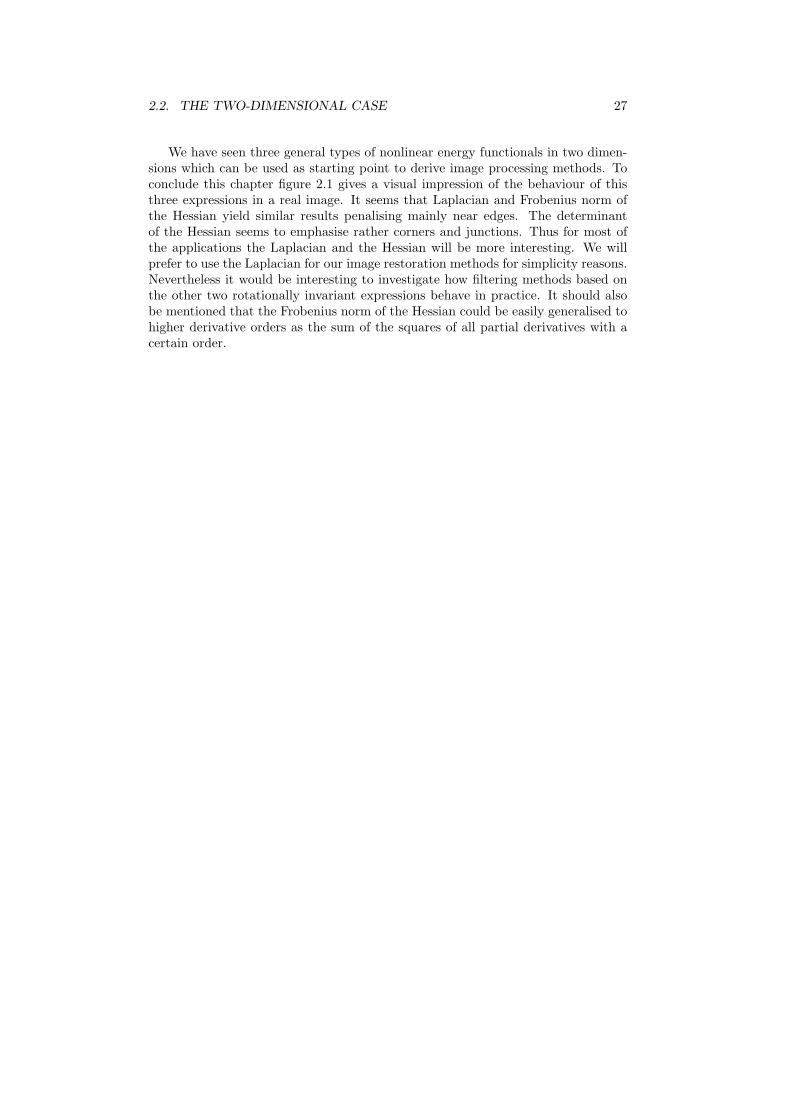
We have seen three general types of nonlinear energy functionals in two dimen-sions which can be used as starting point to derive image processing methods. Toconclude this chapter figure 2.1 gives a visual impression of the behaviour of thisthree expressions in a real image. It seems that Laplacian and Frobenius norm ofthe Hessian yield similar results penalising mainly near edges. The determinantof the Hessian seems to emphasise rather corners and junctions. Thus for most ofthe applications the Laplacian and the Hessian will be more interesting. We willprefer to use the Laplacian for our image restoration methods for simplicity reasons.Nevertheless it would be interesting to investigate how filtering methods based onthe other two rotationally invariant expressions behave in practice. It should alsobe mentioned that the Frobenius norm of the Hessian could be easily generalised tohigher derivative orders as the sum of the squares of all partial derivatives with acertain order.

28 CHAPTER 2. CONTINUOUS ENERGY FUNCTIONALS

Chapter 3
Continuous Filtering
After giving conditions for a minimiser this section will introduce methods that usethese conditions to find one. In our applications a minimiser of an energy functionalis a signal or an image which should be in some way better than the initial one.Thus we consider the resulting image as a filtered version of the initial one and wewill use the notion filtering for the process of minimising the energy functional. Weare interested in the continuous framework in this chapter. Discretisations of thesemethods and the application to concrete problem instances will be described in thenext two chapters.
3.1 Filtering Approaches
As a starting point we discuss different approaches at the example of an energyfunctional that depends on the weighted squares of the derivatives of u. We considera one-dimensional linear energy functional of higher order of the form
E(u) =∫R
((u− f)2 + α
m∑k=1
λk
(dk
dxku
)2)
dx (3.1)
with m ∈ N, λk ∈ R for all k ∈ 1, . . . ,m and α > 0. We integrate over the wholeset R in this case to avoid the influence of boundary conditions.
3.1.1 Direct Minimisation of the Energy Functional
The first approach reformulates the energy functional in the Fourier domain. Thisstrategy is discussed in [18]. Since we use the Fourier transform to simplify theenergy functional this is only applicable for linear penalisers. We can rewrite thefunctional (3.1) using the norm in L2(R) and the linearity of the integral and get
E(u) = ‖u− f‖22 + α
m∑k=1
λk
∥∥∥∥ dk
dxku
∥∥∥∥2
2
. (3.2)
We then apply the Fourier transform to the energy functional. In the followingf denotes the Fourier-Plancherel transform of the function f . For details on thistransform we refer to [33]. With the Plancherel equation the functional can bewritten as
E(u) =∥∥∥u− f
∥∥∥2
2+ α
m∑k=1
λk
∥∥(iξ)ku∥∥2
2
29

30 CHAPTER 3. CONTINUOUS FILTERING
=∥∥∥u− f
∥∥∥2
2+ α
m∑k=1
λk
∥∥ξku∥∥2
2
=∫R
(∣∣∣u− f∣∣∣2 + α
m∑k=1
λk
∣∣ξku∣∣2) dx.
We note that the energy functional in the Fourier domain only depends on |u|2since the derivative operation is transformed into multiplication via the Fouriertransform. From Chapter 2 we see with a decomposition in the real and imaginarypart that the corresponding Euler-Lagrange equation to this functional is given by
0 = Eu = 2(u− f
)+ 2α
m∑k=1
λkξ2ku.
It immediately follows that
f = u + αm∑
k=1
λkξ2ku
which gives us the analytical solution in the Fourier domain
u =
(1 + α
m∑k=1
λkξ2k
)−1
f .
Remark 3.1 It is also possible to compute the Euler-Lagrange equation and thensolve it in the Fourier domain. As a special case of (2.18) we see that the corre-sponding Euler-Lagrange equation to the functional (3.1) is given by
0 = u− f + αm∑
k=1
λk(−1)k dk
dxku(k)
= u− f + α
m∑k=1
(−1)kλku(2k). (3.3)
Applying the Fourier transform then yields:
0 = u− f + αm∑
k=1
λk(−1)kξ2ku
= u− f + α
m∑k=1
λkξ2ku.
It immediately follows that
f = u + αm∑
k=1
λkξ2ku
which gives us the analytical solution in the Fourier domain
u =
(1 + α
m∑k=1
λkξ2k
)−1
f .
In the case of linear filtering we can give analytical solutions with the help of theFourier transform.

3.1. FILTERING APPROACHES 31
3.1.2 Parabolic Differential Equations
Instead of solving the Euler-Lagrange equation directly as in the last section one canalso use iterative methods to approximate a solution. This may seem to be unneces-sary for the linear case since analytical solutions can easily be found. Neverthelesswe will draw our attention on this point to get results which can be generalised tononlinear filtering.
Diffusion Equations
We start with the Euler-Lagrange equation (3.3) and exclude the trivial case α = 0in which the only solution is u = f . With positive α we can write the equation as
u− f
α=
m∑k=1
(−1)k+1λku(2k). (3.4)
In the energy functional the parameter α determines the weight between the sim-ilarity and the smoothness term. Higher values of α lead to smoother solutionswith respect to the actual penalty function. One could also think of filtering asan evolution process and interpret α as a time parameter. Let u(x, t) denote theminimiser of the energy functional with t = α. In this framework the initial signalf is the signal u(·, 0) at time t = 0. This corresponds with the observation that theleft-hand side of equation (3.4) can be interpreted as implicit discretisation of thetime derivative.
We can consider equation (3.4) as fully implicit discretisation of the parabolicdifferential equation
ut =m∑
k=1
(−1)k+1λku(2k)
with initial condition u(x, 0) = f(x) for all x ∈ R and stopping time t = α. We notethat these interpretations are also possible in a nonlinear setting. So the Euler-Lagrange equation from Example 2.10 leads to the nonlinear diffusion equation
ut = (−1)m+1 dm
dxm
(ϕ′((
u(m))2)
u(m)
). (3.5)
Since the quadratic data term (u−f)2 appears in all energy functionals we considerfor signal and image processing, the corresponding Euler-Lagrange equations alwayscontain the linear term u− f . So for every energy functional with a quadratic dataterm we can give a corresponding diffusion equation where the right-hand sidecomes from the smoothness term. This can be immediately carried over to higherdimensional examples.
Diffusion-Reaction Equations
One can also interpret the solution of the Euler-Lagrange equation (3.3) as thesteady state of the diffusion-reaction equation
ut = u− f + αm∑
k=1
(−1)kλku(2k)
with the artificial time variable t and initial condition u(·, 0) = f .In this case one would get the equation
ut = u− f + (−1)mαdm
dxm
(ϕ′((
u(m))2)
u(m)
). (3.6)

32 CHAPTER 3. CONTINUOUS FILTERING
belonging to the Euler-Lagrange equation from example (2.10). To solve the prob-lem with the diffusion-reaction approach one has to reach the steady state efficiently.This can be seen as the main disadvantage compared with the pure diffusion equa-tion: In the diffusion setting the scale parameter α is interpreted as stopping time.In the diffusion-reaction case one has to try to compute the limit for t −→ ∞independent of the value of α.
3.1.3 Generalised Linear Diffusion
In this section we turn our attention to higher order diffusion equations. Theproceeding is similar to the treatment of the diffusion equation in [27].
We have seen in the last section how the functional (3.1) leads to the parabolicdifferential equation
ut =m∑
k=1
(−1)k+1λkd2k
dx2ku (3.7)
with initial condition u(x, 0) = f(x) for all x ∈ R and stopping time t = α. Applyingthe Fourier transform with respect to the x-variable to both sides of this equationyields
ut =m∑
k=1
(−1)k+1λk(−1)kξ2ku
=m∑
k=1
(−1)2k+1λkξ2ku
= −m∑
k=1
λkξ2ku (3.8)
with initial condition u(ξ, 0) = f(ξ) for all ξ ∈ R.We have used the Fourier transform to turn the x-derivatives into algebraic
multiplications. Only the derivative with respect to t is preserved and we obtainan ordinary differential equation with one parameter ξ. The unique solution forequation (3.8) is
u(ξ, t) = exp
(−t
m∑k=1
λkξ2k
)f(ξ) (3.9)
for all t ≥ 0 and all ξ ∈ R.We rewrite equation (3.9) to get some more properties of the solution of equation
(3.8):
u(ξ, t) = exp
(−t
m∑k=1
λkξ2k
)f(ξ)
=
(m∏
k=1
exp(−tλkξ2k
))f(ξ)
= exp(−tλmξ2m
)· . . . · exp
(−tλ1ξ
2)f(ξ). (3.10)
We see that the solution of equation (3.8) can be represented by multiplying theinitial values with exponential functions in the Fourier domain.
Definition 3.2 (Multiplicators) We define the multiplicator functions
Gλk(ξ, t) := exp
(−tλξ2k
)with k ∈ N, λ ∈ R
that appear in the Fourier domain for generalised linear filtering.

3.1. FILTERING APPROACHES 33
If we restrict λ to nonnegative values these functions are bounded:
0 ≤ Gλk(ξ, t) = exp
(−tλξ2k
)≤ 1
for all k ∈ N, t ∈ R+0 and ξ ∈ R.
Remark 3.3 (Stability) Together with equation (3.9) we get an upper bound forthe L2-norm of u(·, t):
‖u(·, t)‖22 =∫R
|u(ξ, t)|2dξ
=∫R
∣∣∣exp(−tλmξ2m
)· . . . · exp
(−tλ1ξ
2)f(ξ)
∣∣∣2 dξ
=∫R
∣∣exp(−tλmξ2m
)∣∣2 · . . . · ∣∣exp(−tλ1ξ
2)∣∣2 |f(ξ)|2dξ
≤∫R
|f(ξ)|2dξ
= ‖f‖22. (3.11)
This shows not only that u(·, t) is in L2 again for initial data in L2: Since themapping Tt : L2 −→ L2, f 7−→ u(·, t) is linear, we have also shown the continuityof Tt.
Together with the Fourier-Plancherel transform F : L2 −→ L2 (see [33, SectionV.2], linear filtering with fixed nonnegative coefficients λ1, . . . , λm and stopping timet can be written as linear continuous operator Tt : L2 −→ L2, f 7−→ F−1TtFf .The Plancherel identity assures that the equivalent inequation to (3.11) holds forthe norm of Ttf = u(·, t) for all t ∈ R+
0 :
‖u(·, t)‖2 = ‖u(·, t)‖2 ≤ ‖f‖2 = ‖f‖2.
We conclude that linear diffusion filtering of higher order is L2-continuous withnorm not greater than 1. That means stability with respect to the L2-norm.
Remark 3.4 (Negative Values for λ) We want to note that these propertiesonly hold for nonnegative coefficients λ1, . . . , λm. The functions
Gλk(ξ, t) = exp
(−tλξ2k
)are unbounded for negative λ. Especially the high frequency components of oursignal f are amplified by multiplying them with exponentially growing functions.Filtering with negative λ1, . . . , λm leads to a rapidly growing L2-norm of the resultu(·, t). Thus the problem is ill-posed for negative filter parameters. For the rest ofthis section we assume the λ1, . . . , λm to be nonnegative.
For t ≥ 0, the functions Gλk(·, t) are in the Schwartz space (see [33]). So their
Fourier backtransform pλk(·, t) exists and is in the Schwartz space, too (see [33,
Lemma V.2.5]). Together with the convolution theorem the solution of equation(3.8) can also be considered as convolution in the spatial domain
u(x, t) =(pλm
m (·, t) ∗ pλm−1m−1 (·, t) ∗ . . . ∗ pλ1
1 (·, t) ∗ f)
(x). (3.12)

34 CHAPTER 3. CONTINUOUS FILTERING
-0.4
-0.2
0
0.2
0.4
0.6
0.8
1
1.2
0 50 100 150 200 250
G with l=1, lambda=1/64, t=1Fourier transform p
-0.4
-0.2
0
0.2
0.4
0.6
0.8
1
1.2
0 50 100 150 200 250
G with l=2, t=1, lambda=1/(8^4)Fourier transform p
-0.4
-0.2
0
0.2
0.4
0.6
0.8
1
1.2
0 50 100 150 200 250
G with l=3, t=1, lambda=1/(8^6)Fourier transform p
-0.4
-0.2
0
0.2
0.4
0.6
0.8
1
1.2
0 50 100 150 200 250
G with l=4, t=1, lambda=1/(8^8)Fourier transform p
-0.4
-0.2
0
0.2
0.4
0.6
0.8
1
1.2
0 50 100 150 200 250
G with l=32, t=1, lambda=1/(8^64)Fourier transform p
Figure 3.1: Gλk(·, t) and corresponding convolution kernels pλ
k(·, t) for k ∈1, 2, 3, 4, 32. The values for λ and t are chosen to visualise the main charac-teristics of the functions.
Definition 3.5 (Convolution Kernels) We define the convolution kernels ap-pearing in generalised linear filtering as
pλk(·, t) := F−1Gλ
k(·, t) for k ∈ N, λ > 0
=∫R
exp(−tλξ2k
)exp (ixξ) dξ.
Figure 3.1 shows some discrete approximations of the functions Gλk(·, t) and the
resulting convolution kernels pλk(·, t) visualised via discrete Fourier transform. We
have used a signal size of 256 pixels. In the case k = 1, we have the well-knownGaussian kernel which has a Gaussian as Fourier transform again. We note that thenonnegativity of the Gaussian corresponds with the minimum-maximum property ofthe corresponding diffusion process. Since higher order kernels pλ
k(·, t) always reachnegative values, the corresponding higher order diffusion will in general violate aminimum-maximum property.

3.1. FILTERING APPROACHES 35
Remark 3.6 From the signals shown in Figure 3.1 one could suppose that thenumber of intervals where pλ
k has negative values is 2(k − 1). It could also bepossible to choose the λk such that the convolution of multiple kernels is positive.This would be the counterpart in the diffusion framework to the positivity resultsfrom [18] for direct minimisation of linear energy functionals. One can also see thatthe discrete versions of the functions Gλ
k get similar to a box function for k −→∞and the functions pλ
k get similar to a sinc function. Perhaps it is possible to proveconvergence in the sense of the L2-norm in the continuous case, too (with the L2-continuity of the Fourier transform, it would suffice to show the convergence foreither Gλ
k or pλk).
We note some scale-space properties of generalised linear filtering. The first onewe have already used in the above remarks:
Proposition 3.7 (Linearity) Generalised linear filtering is a linear operator.
From the convolution representation (3.12) with kernels pλk ∈ C∞ we can derive
that the filtering result is C∞ for L2 initial data:
Proposition 3.8 (Smoothness of the Solution) We consider generalised lin-ear filtering with initial data f ∈ L2(R). Then the solution u is in C∞(R).
Proof: We start with (3.12) and compute the convolution kernel
p = pλmm (·, t) ∗ p
λm−1m−1 (·, t) ∗ . . . ∗ pλ1
1 (·, t).
Then p is in C∞(R), and we can write
d
dxu(x, t) =
∫R
(d
dxp(y − x)
)f(y)dy
which can be iterated and shows the existence of the derivatives of u.
From equation (3.9), the properties of the exponential function and the linearityof the Fourier-Plancherel transform F we can also derive:
Proposition 3.9 (Semigroup-Property of Linear Filtering) The set of gen-eralised linear filtering operators Tt satisfies the semigroup-property
Ts+tf = TsTtf
T0f = f
for all f ∈ L2.
Proposition 3.10 (Invariance of the Average Grey Value) For all t > 0 itis ∫
R
u(x, t)dx =∫R
f(x)dx.
Proof: We keep in mind that the average grey value can be expressed as Fouriercoefficient ∫
R
f(x)dx =∫R
f(x) exp(0ix)dx = f(0).

36 CHAPTER 3. CONTINUOUS FILTERING
Thus we have for all t > 0∫R
u(x, t)dx = u(0, t)
= exp(−tλm0) · . . . · exp(−tλ10)f(0)
= f(0)
=∫R
f(x)dx
which completes the proof.
Proposition 3.11 (Translational Invariance) Generalised linear diffusion fil-tering is translational invariant.
Proof: This statement follows directly from the fact that generalised lineardiffusion can be written as spatial convolution with a kernel p(x, t). Then a substi-tution shows for all a ∈ R
u(x + a, t) =∫R
p (x + a− y, t) f(y)dy
=∫R
p (x− (y − a), t) f(y)dy
=∫R
p (x− y) f (y + a) dy,
which is the claimed translational invariance.
If we restrict ourselves to only one derivative order we have also scale invariance.
Proposition 3.12 (Scale Invariance) If the function f is scaled with σ > 0 thenthere is a t > 0 such that (
Ttf( ·
σ
))(x) = (Ttf(·))
(x
σ
)holds.
Proof: First we note that with the substitution y = yσ(
Ttf( ·
σ
))(x) =
∫R
pλk(x− y, t)f
( y
σ
)dy
= σ
∫R
pλk(x− σy, t)f(y)dy. (3.13)
We observe that with Definition 3.5 and a second substitution
pλk(x− σy, t) =
∫R
exp(−tλξ2k
)exp (i(x− σy)ξ) dξ
=1σ
∫R
exp(− t
σ2kλξ2k
)exp
(i(x
σ− y)
ξ)
dξ
=1σ
pλk
(x
σ− y,
t
σ2k
).

3.2. NONLINEAR DIFFUSION OF SECOND ORDER 37
Using this in equation (3.13) yields(Ttf
( ·σ
))(x) =
∫R
pλk
(x
σ− y,
t
σ2k
)f(y)dy
=(T t
σ2kf)(x
σ
)which proves the claimed scale-invariance.
We note that the convolution with pλk(·, t) has been axiomatically derived by
Iijima in [16]. He starts with demanding linearity, translational and scale invarianceand the semigroup property and obtains the convolution with pλ
k(·, t). More on thesescale-space axiomatics can be found in [32].
3.2 Nonlinear Diffusion of Second Order
Let us now turn our attention to nonlinear energy functionals of derivative order 2in one dimension. Such functionals can be written in the following form:
E(u) =∫R
((u− f)2 + αϕ
(u2
xx
))dx. (3.14)
We assume that ϕ ∈ C3(R), that means it is three times continuous differentiable.Further we demand that it satisfies the condition ϕ(0) = 0 to ensure that the integralconverges at least for constant or linear argument functions u. The correspondingEuler-Lagrange equation to (3.14) is the elliptic equation
u− f
α= − d2
dx2
(ϕ′(u2
xx
)uxx
).
As we have discussed in Section 3.1.2 this can be interpreted as a fully implicitdiscretisation of the parabolic partial differential equation
ut = − d2
dx2
(ϕ′(u2
xx
)uxx
)(3.15)
with initial condition u(0, x) = f(x) and stopping time t = α. We now expand theright-hand side of this equation. Using
d
dx
(ϕ′(u2
xx
)uxx
)=
[d
dxϕ′(u2
xx
)]uxx + ϕ′
(u2
xx
) [ d
dxuxx
]= 2ϕ′′
(u2
xx
)u2
xxuxxx + ϕ′(u2
xx
)uxxx
=(2ϕ′′
(u2
xx
)u2
xx + ϕ′(u2
xx
))uxxx
we obtain
d2
dx2
(ϕ′(u2
xx
)uxx
)=
[d
dx
(2ϕ′′
(u2
xx
)u2
xx + ϕ′(u2
xx
))]uxxx
+[2ϕ′′
(u2
xx
)u2
xx + ϕ′(u2
xx
)]uxxxx
= 2[(
d
dxϕ′′(u2
xx
))u2
xx + ϕ′′(u2
xx
)( d
dxu2
xx
)+ϕ′′
(u2
xx
)uxxuxxx
]uxxx
+[2ϕ′′
(u2
xx
)u2
xx + ϕ′(u2
xx
)]uxxxx

38 CHAPTER 3. CONTINUOUS FILTERING
=[ϕ′′′(u2
xx
)2u3
xxuxxx + ϕ′′(u2
xx
)2uxxuxxx
+ϕ′′(u2
xx
)uxxuxxx
]2uxxx
+[2ϕ′′
(u2
xx
)u2
xx + ϕ′(u2
xx
)]uxxxx
=[2u2
xxx
(2ϕ′′′
(u2
xx
)u2
xx + 3ϕ′′(u2
xx
))]uxx
+[2ϕ′′
(u2
xx
)u2
xx + ϕ′(u2
xx
)]uxxxx.
Introducing the abbreviations
Φ1(x2) := 2ϕ′′′(x2)x2 + 3ϕ′′(x2)Φ2(x2) := 2ϕ′′(x2)x2 + ϕ′(x2) (3.16)
allows us to rewrite equation (3.15) as follows:
ut = − d2
dx2
(ϕ′(u2
xx
)uxx
)= −
(2u2
xxxΦ1
(u2
xx
))uxx − Φ2
(u2
xx
)uxxxx. (3.17)
As we have seen in Section 3.1.3 the well-posedness of diffusion processes dependson the signs of the factors in front of uxx and uxxxx. We now consider the nonlinearterms −2u2
xxxΦ1
(u2
xx
)and Φ2
(u2
xx
)as coefficients of uxx and uxxxx and we are
therefore interested in the signs of these terms.In regions where u2
xxx 6= 0 the signs only depend on the functions Φ1 and Φ2
which involve the first three derivatives of the penalty function ϕ. Note that theexpression Φ2(x2) as defined in (3.16) also appears in the consideration of first orderfiltering to distinguish between forward and backward diffusion. So the highestdiffusion order will behave like the first order diffusion in a standard first ordersetting. The third derivative uxxx appears only quadratic and therefore cannotchange the sign. It can be seen as a weight parameter on the first order diffusionprocess. We keep in mind that we only obtain necessary conditions for first orderforward or backward diffusion.
The conditions on Φ1 and Φ2 can be summarised as follows:
Φ1
(u2
xx
)< 0 first order forward diffusion (well-posed)
Φ1
(u2
xx
)> 0 first order backward diffusion (ill-posed)
Φ2
(u2
xx
)> 0 second order forward diffusion (well-posed)
Φ2
(u2
xx
)< 0 second order backward diffusion (ill-posed).
3.3 Application to Penalty Functions
Let us now investigate some commonly used penalisers ϕ and study their effecton corresponding second order diffusions. The investigated penalisers are alreadymentioned in the first chapter. More references can be found there.
3.3.1 Linear Filtering
A linear filter is obtained with ϕ(x) := cx for some c ∈ R and all x ∈ R.With ϕ′(x) = c and ϕ′′(x) = ϕ′′′(x) = 0 it immediately follows that Φ1(x) = 0 andΦ2(x) = c hold for all x ∈ R. Only the highest diffusion order is kept in this case.The corresponding parabolic differential equation is
ut = −c uxxxx.
For c > 0, linear filtering leads to a well-posed second-order forward diffusion.

3.3. APPLICATION TO PENALTY FUNCTIONS 39
3.3.2 Charbonnier
The Charbonnier filter with
ϕ(x) := 2λ2
(√1 +
x
λ2− 1)
with λ ∈ R+, x ∈ R+0
leads to forward diffusion in the first order filtering framework. Note that theargument x will be always nonnegative in energy functionals of the form (3.14)since the penalty depends on the square of the second derivative of our data u. Wewill now derive that its behaviour is exactly the same in a second order filter.
The first three derivatives of ϕ are:
ϕ′(x) =(1 +
x
λ2
)− 12
ϕ′′(x) =−12λ2
(1 +
x
λ2
)− 32
ϕ′′′(x) =3
4λ4
(1 +
x
λ2
)− 52
.
We then derive our sign functions as defined in (3.16):
Φ1(x2) =3x2
2λ4
(1 +
x2
λ2
)− 52
+−32λ2
(1 +
x2
λ2
)− 32
=−32λ2
(1 +
x2
λ2
)− 52
< 0 for all x ∈ R and
Φ2(x2) =−2x2
2λ2
(1 +
x2
λ2
)− 32
+(
1 +x2
λ2
)− 12
=(
1 +x2
λ2
)− 32
> 0 for all x ∈ R.
The Charbonnier filter of second order always performs forward diffusion.
3.3.3 Perona-Malik
Let us consider the classical Perona-Malik penalty function
ϕ(x) := λ2 ln(1 +
x
λ2
)with x ∈ R+
0 , λ ∈ R+.
The Perona-Malik function has the property to lead to forward-backward diffusionin first order filtering methods. The parameter λ is the limit to distinguish betweenforward diffusion (for |ux| < λ) and backward diffusion (for |ux| > λ). Thus λ playsthe role of a contrast parameter. Choosing a suitable value for λ allows to smoothin the interior of a region (where |ux| < λ), while enhancing edges (with |ux| < λ)by means of backward diffusion. We will see that the behaviour in the second-ordercase is not that easy to describe.
Computation of the first three derivatives of our penalty function yields
ϕ′(x) =(1 +
x
λ2
)−1
ϕ′′(x) =−1λ2
(1 +
x
λ2
)−2
ϕ′′′(x) =2λ4
(1 +
x
λ2
)−3
.

40 CHAPTER 3. CONTINUOUS FILTERING
Then we consider the sign determining functions Φ1 and Φ2.
Φ1(x2) = 2ϕ′′′(x2)x2 + 3ϕ′′(x2)
=4x2
λ4
(1 +
x2
λ2
)−3
+−3λ2
(1 +
x2
λ2
)−2
=x2 − 3λ2
λ4(1 + x2
λ2
)3Φ2(x2) = 2ϕ′′(x2)x2 + ϕ′(x2)
=−2x2
λ2
(1 +
x2
λ2
)−2
+(
1 +x2
λ2
)−1
=λ2 − x2
λ2
(1 +
x2
λ2
)−2
We see that the term Φ2 for the fourth derivative order leads to the well-knowncondition from first order filtering (with the difference that this function dependson the square of the second and not of the first derivative.)
Φ2(x2) > 0 ⇐⇒ x2 < λ2 ⇐⇒ |x| < λ
We have second order forward diffusion in regions where |uxx| < λ and second orderbackward diffusion if |u2
xx| > λ.The first order diffusion depends on Φ1:
Φ1(x2) < 0 ⇐⇒ x2 − 3λ2 < 0 ⇐⇒ x2 < 3λ2 ⇐⇒ |x| <√
3λ.
So this term may lead to forward first order diffusion in the case that |u2xx| <
√3λ
and to backward first order diffusion if it is greater. We conclude that the behaviourof second-order Perona-Malik filtering can be divided into three cases:
|uxx| < λ forward diffusion of first and second order(well-posed)
λ < |uxx| <√
3λ forward diffusion of first order andbackward diffusion of second order
|uxx| >√
3λ backward diffusion of first and second order(ill-posed).
3.3.4 Total Variation Approximations
As next example we consider approximations of the total variation function. We fixε > 0 and consider the regularised total variation penaliser
ϕ(x) := 2√
(ε2 + x)− 2ε for x ∈ R+0 .
We need to subtract the constant term 2ε to get ϕ(0) = 0. As in the above exampleswe need the derivatives of ϕ at first; these are
ϕ′(x) =(ε2 + x
)− 12
ϕ′′(x) =−12(ε2 + x
)− 32
ϕ′′′(x) =34(ε2 + x
)− 52 .

3.3. APPLICATION TO PENALTY FUNCTIONS 41
According to formula (3.16) we compute the coefficient functions
Φ1(x2) =3x2
2(ε2 + x2
)− 52 +
−32(ε2 + x2
)− 32
=−3ε2
2(ε2 + x2
)− 52 < 0 for all x ∈ R and
Φ2(x2) =−2x2
2(ε2 + x2
)− 32 +
(ε2 + x2
)− 12
= ε2(ε2 + x2
)− 32 > 0 for all x ∈ R.
We deduce that regularised total variation approximations always perform for-ward diffusion. In the case the second derivative |uxx| is small the value of ε playsan important role: The limits of our two functions are
limx−→0
Φ1(x2) = limx−→0
−32· ε2
√ε2 + x2
5 = −32ε−3
and
limx−→0
Φ2(x2) = limx−→0
ε2
√ε2 + x2
3 =1ε.
We see that the value of ε for the TV-approximation is very important for the speedof the diffusion in regions with small second derivative.
3.3.5 Total Variation
Instead of the approximation we now consider the TV functional itself. We use thepenaliser ϕ(x) = 2
√x for x ∈ R+
0 . The derivatives of ϕ
ϕ′(x) = x−12
ϕ′′(x) = −12x−
32
ϕ′′′(x) =34x−
52
are only defined for x ∈ R+. Our coefficient functions then are
Φ1(x2) =32(x2)−
52 x2 − 3
2(x2)−
32
=32x−3 − 3
2x−3
= 0 for all x ∈ R+ and
Φ2(x2) = −(x2)−32 x2 + (x2)−
12
= −x−1 + x−1
= 0 for all x ∈ R+.
We see that the total variation method is exactly the border case between forwardand backward diffusion. Since the derivatives are not defined for x = 0 the methodis usually approximated as mentioned above for practical implementations.

42 CHAPTER 3. CONTINUOUS FILTERING

Chapter 4
Discretisation
After studying methods for minimisation in the continuous setting we want to carryover these to the discrete domain. At first we will take a look at two ways toapproximate the derivative only involving the function’s values at discrete points:the finite differences and spectral methods. Both of them will be used in the noiseremoval methods described in this thesis.
4.1 General Remarks and Notations
First we like to introduce some general notations that will be used throughout thischapter.
In the one-dimensional continuous case we usually consider energy functionalswith an interval Ω = (a, b) with a, b ∈ R, b > a as integration domain. Our dataand results are functions f : [a, b] −→ R. For discrete methods we choose a signallength n ∈ N and replace the interval by equidistant grid points
Ωh := xi | i = 0, . . . , n− 1 withxi := a + ih for i ∈ 0, . . . , n− 1,
where h := b−an−1 is our spatial step size. We substitute the function f by a vector
f ∈ Rn containing the values of f at these grid points
f := (f(x0), . . . , f(xn−1))T .
This vector will always be denoted with the letter of the corresponding function inbold print. Extending this vector at both sides with zeros, one can represent it alsoas an infinite sequence. It is clear that this sequence belongs to the spaces
`p(Z) :=
(ξk)k∈Z ⊂ R;
∑k∈Z
|ξk|p < ∞
for all p ∈ N since it is bounded and only a finite number of entries is nonzero.This extension can be useful to write finite differences as linear operators or asconvolution. We are especially interested in the space `2(Z) since is is a Hilbertspace with the scalar product
〈f ,g〉 =∑k∈Z
fkgk.
We introduce some common operators on this space that will be useful to expressfinite difference methods.
43

44 CHAPTER 4. DISCRETISATION
Definition 4.1 (Left and Right Shift) We define the left shift operator
L : `2(Z) −→ `2(Z), (Lf)k = fk+1 for all k ∈ Z,
and the right shift operator
R : `2(Z) −→ `2(Z), (Rf)k = fk−1 for all k ∈ Z.
The following lemma summarises some useful and simple properties of the shiftsthat we will use later on:
Lemma 4.2 (Properties of Shifts) For L and R defined as above the followingproperties hold:
1. The left and the right shift are adjoint operators, i. e. for all f ,g ∈ `2(Z) theidentity 〈Lf ,g〉 = 〈f , Rg〉 holds.
2. The left and the right shift are inverse to each other, i. e. LR = RL = I. Inparticular the operators L and R commute.
We also define a subspace of `2(Z) isomorphic to Rn such that we can use the theoryin our practical examples with finite Ωh.
Definition 4.3 (Mn and Orthogonal Projections) Let n ∈ N. We define
Mn :=(ξk)k∈Z ∈ `2(Z) | ξk = 0 for all k 6∈ 0, . . . , n− 1
as the subspace of `2(Z) of all sequences for which only the entries with indices0, . . . , n − 1 may be nonzero. With PMn : `2(Z) −→ Mn we denote the orthogonalprojection onto Mn.
It is clear that Mn is isomorphic to Rn. We would also note that as orthogonalprojection the operator PMn is self-adjoint. These notions will be useful to obtainmatrix representations for the results in `2(Z).
With `∞(Z) we denote the space of all bounded real sequences over Z. Theextension of f can also be regarded as a sequence in `∞. For details on this sequencespaces we refer to introductions on functional analysis like [13] or [33]. We will seethat in the case of spectral methods a periodic extension of the vector to a sequencein `∞(Z) is the natural proceeding.
In this work we also consider two-dimensional examples with integration domainΩ = (a, b)×(c, d) ⊂ R2 with a, b, c, d ∈ R, b > a, d > c. This domain will be replacedby an equidistant rectangular grid of the form
Ωh := (xi, yj) | i = 0, . . . , nx − 1 and j = 0, . . . , ny − 1 withxi := a + ihx for i ∈ 0, . . . , nx − 1yj := b + jhy for j ∈ 0, . . . , ny − 1,
where hx := b−anx−1 and hy := d−c
ny−1 are the spatial step sizes in the coordinate axisdirections. The values of a function f : Ω −→ R on the set Ωh could be written asa matrix f ∈ Rnx×ny with entries fij = f(xi, yj). Instead we prefer to embed thevalues in the vector f ∈ Rnxny with
fi+jnx= f(xi, yj), i = 0, . . . , nx − 1, j = 0, . . . , ny − 1.
So we are able to write noise removal methods as matrix-vector multiplications.Before we are able to talk about discrete noise removal methods we need some
background on the approximation of derivatives. We will summarise the mainresults concerning two different ways to approximate a derivative.

4.2. FINITE DIFFERENCES 45
4.2 Finite Differences
Finite differences are the commonly used way to approximate derivatives. The mainidea is to approximate differential quotients f ′(x) = lim
h−→∞f(x+h)−f(x)
h by suitable
difference quotients.
Definition 4.4 (Forward, Backward and Central Difference) Let h > 0 bean arbitrary step size, x ∈ R, and f : [x− h, x + h] −→ R. We define the forwarddifference (
D+h f)(x) :=
f(x + h)− f(x)h
,
the backward difference
(D−
h f)(x) :=
f(x)− f(x− h)h
and the symmetric or central difference
(D0
hf)(x) :=
f(x + h)− f(x− h)2h
.
If f is sufficient smooth (in this case C2) the Taylor formula
f(x + h) = f(x) + hf ′(x) +12h2f ′′(ξ) for ξ ∈ (x, x + h)
yields the error estimate (D+
h f)(x) = f ′(x) + O(h)
expressed with the Landau symbol. The error is linear in h. The backward differencehas the same accuracy order as the forward difference. The central difference evenyields a quadratic convergence behaviour for h −→ 0. We note that
(D+
h f)(x) =
f(x + h)− f(x)h
=(D0
h/2f)(
x +h
2
)and so the forward difference of f at the point x with step size h can also beconsidered as an approximation for f ′
(x + h
2
)of second order.
Iterating the forward difference yields approximations for higher derivatives:
(D+
h D+h f)(x) =
(D+
h f)(x + h)−
(D+
h
)(x)
h
=f(x + 2h)− 2f(x + h) + f(x)
h2
≈ f ′′(x + h).
It is useful to write the forward difference as linear operator to generalise theiteration and to get some statements concerning boundary conditions. The ideaof this can be found in [4] and [14], for example, where calculations with operatorsymbols for differences are performed. We use the vector notation for the valuesof f at the grid points Ωh = x, x + h, . . . , x + mh as indicated in the preceedingsection and set f = (f(x), . . . , f(x + mh)). Extending f to both sides with zeroentries makes a sequence in `2(Z) out of it. The pointwise forward and backwarddifferences now can be written as linear operator on `2:

46 CHAPTER 4. DISCRETISATION
Definition 4.5 (Difference Operators) We consider the pointwise forward dif-ference operator D+
h : `2(Z) −→ `2(Z) defined by
(D+
h f)k
=fk+1 − fk
hfor all k ∈ Z.
The pointwise backward difference operator D−h : `2(Z) −→ `2(Z) is analogously
defined by (D−
h f)k
=fk − fk−1
hfor all k ∈ Z.
Alternatively we can write the pointwise forward and backward difference in termsof shift operators and the identity operator:
Lemma 4.6 (Differences with Shift Operators) The forward difference oper-ator can be written as the difference of a left shift operator and the identity I scaledwith 1
h :
D+h =
1h
(L− I). (4.1)
The backward difference operator is
D−h =
1h
(I −R) = RD+h . (4.2)
We now calculate powers of D+h and D−
h to get higher differences and approxi-mations of higher derivatives.
Lemma 4.7 (Higher Differences) The higher differences can be calculated as
(D+
h
)m=
1hm
m∑l=0
(−1)m−l(m
l
)Ll and(
D−h
)m= Rm
(D+
h
)m.
Proof: With the observation that L and I commute, we get by taking powersof equation (4.1) with the binomial formula(
D+h
)m=
1hm
(L− I)m
=1
hm
m∑l=0
(m
l
)Ll(−I)m−l
=1
hm
m∑l=0
(−1)m−l(m
l
)Ll.
The second statement follows from equation (4.2). With Lemma 4.2 it is clear thatthe shifts and the difference operators commute and therefore(
D−h
)m=(RD+
h
)m= Rm
(D+
h
)mwhich is our second statement.
From Lemma 4.7 we obtain the coefficients for the values of f that are needed tocompute an approximation of the mth derivative at the point x:
((D+
h
)mf)0
=m∑
l=0
(−1)m−l
hm
(m
l
)fl.

4.2. FINITE DIFFERENCES 47
We see that the mth finite difference is a linear combination of the values of f at them + 1 points x, x + h, . . . , x + mh. The coefficients of these values are the binomialcoefficients divided by hm and with alternating signs such that the last summand1
hm f(x + mh) has positive sign.
Remark 4.8 (Approximation of Higher Derivatives) The property that thisexpression
((D+
h
)mf)(x) computed of the values of f at the m+1 equidistant points
x, . . . , x + mh yields an approximation for f (m) at the central point(x + mh
2
)is
mentioned in [14] and [24], for example. A proof based on polynomial interpolationcan be found in [24].
The next remark yields an interpretation of finite differences in terms of local poly-nomial interpolation. It should point out the approach behind finite differences incomparison to the spectral methods presented in the next section.
Remark 4.9 (Differences and Local Interpolation) The first forward differ-ence can also be seen as the exact derivative of the local interpolation of f with apolynomial of degree 1 at an arbitrary point between x and x + h. Analogously toget the mth forward difference a local interpolation polynomial p of degree m withthe m + 1 equidistant grid points x, x + h, . . . , x + mh is build. The mth derivativeof p at the point x + mh
2 is the mth difference. We refer to [24] for details.
Lemma 4.10 (Adjoint Operator) For the mth forward difference(D+
h
)mwe get
the adjoint operator(−D−
h
)m.
Proof: For all f ,g ∈ `2 Lemma 4.2 and Lemma 4.6 show that
〈(D+
h
)mf ,g〉 =
1hm
〈(L− I)mf ,g〉
=1
hm〈f , (R− I)mg〉
= 〈f ,(−D−
h
)mg〉,
and so we get the adjoint operator as given above.
Remark 4.11 (Finite Differences as Convolution) The iterated finite differ-ence operator
(D+
h
)m: `2(Z) −→ `2(Z) from the proof of Lemma 4.7 is linear and
shift invariant. Thus can also be expressed as a discrete convolution
(dm ∗ f)k =∑l∈Z
dmk−lfl
with the convolution kernel
dml =
(−1)m−l
hm
(lm
)if − l ∈ −m, . . . , 0
0 else.
This notation can also be used to deduce implementations of different boundaryconditions with discrete methods.
We will give two examples for these notation. The component with index 0 isbold printed.
d+h =
1h
(. . . , 0, 1, -1, 0, . . .) .
48 CHAPTER 4. DISCRETISATION
We see that the convolution with d+h yields a sequence consisting of the forward
differences of f at the points xl for all l ∈ Z:
(d+
h ∗ f)l=∑k∈Z
(d+
h
)l−k
fk =fl+1 − fl
h=(D+
h f)(xl).
The approximation for the second derivative written as convolution stencil lookslike this:
d2h =
1h2
(. . . , 0, 1,−2,1, 0, . . .) .
When we consider finite differences as exact derivatives of polynomials it is clearhow they should behave if the considered function f is a polynomial. The followingproposition and remark will confirm this assumption.
Proposition 4.12 (First Difference of Polynomials) Let p be a real polyno-
mial of degree m ∈ N, i. e. p(x) =m∑
k=0
akxk with ak ∈ R for all k ∈ 0, . . . ,m and
am 6= 0. Let h > 0 be an arbitrary step size and x ∈ R. The forward difference of pwith step size h is a polynomial of degree m− 1.
Proof: We compute the forward difference with step size h of p at point x
(D+
h p)(x) =
p(x + h)− p(x)h
=1h
m∑k=0
ak
((x + h)k − xk
)=
1h
m∑k=0
ak
((k∑
l=0
(k
l
)xk−lhl
)− xk
)
=1h
m∑k=0
ak
(k∑
l=1
(k
l
)xk−lhl +
(k
0
)xkh0 − xk
)
=1h
m∑k=0
k−1∑l=0
ak
(k
l + 1
)xk−1−lhl
The exponent of x gets maximal for l = 0 and k = m. The summand with thehighest exponent of x is
am
(m
1
)xm−1h0 = m am xm−1
and does not vanish since we assumed that am 6= 0. This computation does notmake any use of the particular point x. We conclude that the forward difference ofa polynomial of degree m is a polynomial of degree m− 1.
Remark 4.13 (Higher Differences of Polynomials) One can also get a state-ment about higher differences of polynomials: Iterating the argumentation from thepreceeding lemma shows that the mth forward difference of a polynomial of degreem is constant (or a polynomial of degree 0). The above computations even allowus to give the exact value of this difference which is m! am. It is clear that the(m + 1)th difference will vanish.
4.2. FINITE DIFFERENCES 49
4.2.1 Matrix Notation
As already indicated above we also introduce a matrix notation for finite differencederivative approximation. By multiplying the matrix DF
1,n ∈ R(n−1)×n defined by
DF1,n :=
1h
−1 1 0 . . . 0
0 −1 1. . .
......
. . .. . .
. . . 00 . . . 0 −1 1
with a vector f , the product
DF1,nf =
(f(x2)− f(x1)
h, . . . ,
f(xn)− f(xn−1)h
)yields an approximation of the derivative f ′ at the equidistant grid points
x1 + x2
2, . . . ,
xn−1 + xn
2.
The F in DF1,n stands for derivative approximation with Finite differences. For a
second derivative approximation we iterate the first derivative taking care of theright matrix dimensions and get
DF1,n−1D
F1,nf =
(f(x3)− 2f(x2) + f(x1)
h2, . . . ,
f(xn)− 2f(xn−1) + f(xn−2)h2
).
This approximates the second derivative f ′′ at the grid points x2, . . . , xn−1. Wedefine the matrix DF
2,n ∈ R(n−2)×n as
DF2,n = DF
1,n−1DF1,n =
1h2
1 −2 1 0 . . . 0
0 1 −2 1. . .
......
. . .. . .
. . .. . . 0
0 . . . 0 1 −2 1
.
This can be extended to higher orders with the
Definition 4.14 (Finite Differences as Matrix) For n ∈ N \ 0 we define thefinite difference derivative approximation of order m ∈ 1, . . . , n − 1 as the (n −m)× n - matrix
DFm,n = DF
1,n−m+1 · . . . ·DF1,n.
Remembering Remark 4.8 we note that multiplying the matrix DFm,n with a vector
f ∈ Rn
DFm,n
f0...
fn−1
=
((
D+h
)mf)0
...((D+
h
)mf)n−1−m
≈
f (m)(x0 + mh
2
)...
f (m)(xn−1−m + mh
2
)
yields an approximation of the mth derivative of f at the points
x0 +mh
2, x1 +
mh
2, . . . , xn−1−m +
mh
2.
To deduce an upper bound for the spectral norm we use the theorem of Gershgorin(see [26], theorem 6.9.4).
50 CHAPTER 4. DISCRETISATION
Theorem 4.15 (Gershgorin) The union of all discs
Ki :=
µ ∈ C; |µ− aii| ≤n∑
k=1k 6=i
|aik|
for i = 1, 2, . . . , n
contains all eigenvalues of the n× n matrix A = (aik).
We use this to prove the following
Lemma 4.16 (Spectral Norm Estimate) For the spectral norm of the matrixDF
m,n the inequality ∥∥DFm,n
∥∥2≤ 2m
hm
holds.
Proof: First we consider the spectral norm of DF1,n. We see that
(DF
1,n
)TDF
1,n =1h2
1 −1 0 . . . 0
−1 2 −1. . .
...
0. . .
. . .. . . 0
.... . . −1 2 −1
0 . . . 0 −1 1
,
and with the Theorem 4.15 of Gershgorin we state that
σ((
DF1,n
)TDF
1,n
)⊆
µ ∈ C;∣∣∣∣µ− 2
h2
∣∣∣∣ ≤ 2h2
∨∣∣∣∣µ− 1
h2
∣∣∣∣ ≤ 1h2
where σ denotes the set of all eigenvalues (the spectrum). As a product of the formAT A the matrix is also symmetric and therefore all eigenvalues are real, and we get
σ((
DF1,n
)TDF
1,n
)⊆[0,
4h2
].
For the spectral radius of DF1,n this means
∥∥DF1,n
∥∥2≤ 2
h.
We state that this estimate is independent of the dimension n. Since the spectralnorm is submultiplicative we state that∥∥DF
m,n
∥∥2
≤∥∥DF
1,n−m+1
∥∥2· . . . ·
∥∥DF1,n
∥∥2
≤ 2m
hm,
and the estimate is proven.
Remark 4.17 (Restriction of the Operator) We can also understand the ma-trix DF
m,n as a restriction of the pointwise forward difference operator(D+
h
)monto
the space Mn−m from Definition 4.3. Identifying Rn with Mn we can write thematrix as the operator
PMn−m
(D+
h
)m.

4.2. FINITE DIFFERENCES 51
Remark 4.18 (Transposed Matrix and Boundary Conditions) We will usethe matrix DF
m,n in discrete energy functionals in Section 5.1. In the gradient of
such a functional the transposed matrix(DF
m,n
)T occurs in a natural way. Wewould like to understand some more properties of this matrix. Since it is a matrixwith real entries it can be expressed as adjoint operator of the matrix DF
m,n. Thuswe consider with Lemma 4.10 and Lemma 4.7 the adjoint operator(
PMn−m
(D+
h
)m)∗= (−1)m
(D−
h
)mPMn−m
= (−1)mRm(D+
h
)mPMn−m .
Basically this is a shifted version of the mth difference multiplied with (−1)m. Wewould like to investigate in detail how this operator acts on a sequence f : Theprojection PMn−m maps all entries fk of f with indices k 6∈ 0, . . . , n − m − 1 tozero. Using the formula from Lemma 4.7 it follows that((
D+h
)mPMn−mf
)k
=m∑
l=0
(−1)m−l
hm
(m
l
)(PMn−mf)k+l
=m∑
l=0
(−1)m−l
hm
(m
l
)fk+l
=((
D+h
)mf)k
for all k ∈ 0, . . . , n− 2m− 1.
For k ≤ −m− 1 or k ≥ n−m we can also state that((D+
h
)mPMn−mf
)k
= 0,
since only zero entries of PMn−mf are taken into consideration to compute the mthdifference. The interesting regions are now −m ≤ k ≤ −1 and n−m + 1 ≤ k ≤ n.Here nonzero entries of f may occur, and also zeros generated by the projection areinvolved. One could consider the values calculated there as approximation of themth derivative of f under the assumption of further conditions. For example it is((
D+h
)mPMn−mf
)−1
=((
D+h
)mf)−1− (−1)m
hmf−1.
Since (−1)m
hm is nonzero, the value((
D+h
)mPMn−mf
)−1
can be considered as theapproximation of f (m)
(x0 + mh
2
)under the assumption that f(x−1) = 0.
More generally for k ∈ 1, . . . ,m it is
((D+
h
)mPMn−mf
)−k
=((
D+h
)mf)−k−
k−1∑l=0
(−1)m−l
hm
(m
l
)fl−k.
We can state that((
D+h
)mPMn−mf
)−k
can be considered as the approximation off (m)
(x−k + mh
2
)under the assumption that
k−1∑l=0
(−1)m−1
hm
(m
l
)fl−k = 0.
We interpret this assumption as a discretisation of the condition
f (k−1)(ξ) = 0 for ξ ∈(
x0, x0 −mh
2
)what can be understood as the discrete version of the boundary condition
f (k−1)(a) = 0
for the left boundary a of our interval. These considerations can be made for theright boundary in the same way.

52 CHAPTER 4. DISCRETISATION
4.2.2 Finite Differences and Polynomial Data Fitting
We would like to further investigate the connection between polynomials and finitedifferences. Assume that the coefficients a0, . . . am−1 of a polynomial
p(x) =m−1∑i=0
aixi
of degree m−1 are given. The evaluation of p at a given point x ∈ R can be writtenas the scalar product of the two vectors a, x ∈ Rm defined as
a := (a0, a1, . . . , am−1)x :=
(x0, x1, . . . , xm−1
).
Taking the scalar product of a with different x means evaluating the polynomialat different points. For n ≥ m we define the submatrices V m
n ∈ Rn×m of theVandermonde matrix as
V mn :=
1 x0 x2
0 . . . xm−10
1 x1 x21 . . . xm−1
1...
......
...1 xn−1 x2
n−1 . . . xm−1n−1
.
The matrix-vector product V mn a yields the evaluation of the polynomial p repre-
sented by its coefficients in a evaluated at the points x0, . . . , xn−1.Conversely, one can start with grid points x0, . . . , xn−1 and given values y :=
(y0, . . . , yn−1)T . If there exists a polynomial p of degree less than m with p(xi) = yi
for all i ∈ 0, . . . , n−1 it can be found as the solution of the linear equation system
V mn a = y.
If the points x0, . . . , xn−1 are pairwise different the matrix V kn has full rank m and if
a solution exists it is unique. For details on matrices of Vandermonde type refer to[15] and [35]. If no solution exists we can solve the according least square problem
mina∈Rn
‖V mn a− y‖2
to get the best possible solution in the sense of least squares. It is well-known thatthis least-square approximation can be expressed as the orthogonal projection of yonto the range of V k
n , i. e.a∗ = Pran(V m
n )y.
We refer to [26] for more information on the topic least-square data fitting andgeneralised inverse.
The following proposition builds up the link between finite differences and leastsquare polynomial data fitting:
Proposition 4.19 (Kernel of DFn,m) The kernel of the finite difference approxi-
mation matrix DFm,n is the subspace of Rn consisting of all equidistant polynomial
evaluations for polynomials with degree less than m, i. e.
ker(DF
m,n
)= ran (V m
n ) .
Proof: First we show that ran (V mn ) ⊆ ker
(DF
m,n
). We start with y ∈
ran (V mn ). There exists a polynomial p of degree less than m with p(xi) = yi.

4.2. FINITE DIFFERENCES 53
It follows from Proposition 4.12 that applying the forward difference k times yieldszero, and y is in the kernel of DF
m,n.Now we show the opposite direction ker
(DF
m,n
)⊆ ran (V m
n ). Assume y ∈ker(DF
m,n
)and y is a function with the interpolation property
y(xi) = yi for all i ∈ 0, . . . , n− 1.
From the definition of DFm,n we know that this is equivalent to((
D+h
)my)(x) = 0 for all x ∈ x1, . . . , xn−m
and for any function y with the interpolation property
y(xi) = yi for all i ∈ 0, . . . , n− 1.
Since the higher differences((
D+h
)ky)
(x0) with k ∈ m + 1, . . . , n − 1 can beexpressed as linear combinations of the differences with order m, we see that((
D+h
)ky)
(x0) = 0 for all k ∈ m + 1, . . . , n− 1.
It is well-known that there exists a polynomial p(x) =n−1∑k=0
akxk of degree less than
n with the interpolation property
p(xi) = yi for all i ∈ 1, . . . , n.
This polynomial is uniquely determined. Applying the forward difference n − 1times yields a constant (
D+h
)n−1p = (n− 1)! an−1.
Since the difference is zero, the leading coefficient also vanishes, and the degree of p
is less than n−1. We can iterate this argumentation as long as the difference(D+
h
)lis zero. It follows that p has degree less than or equal m− 1. This is equivalent toour claim that y ∈ ran (V m
n ).
4.2.3 Neumann Boundary Conditions
In image processing problems often Neumann boundary conditions are assumed.We have already seen a derivative approximation of second order with Neumannboundary conditions in the proof of Lemma 4.16. The matrix
DFN2,n := −
(DF
1,n
)TDF
1,n =1h2
−1 1 0 . . . 0
1 −2 1. . .
...
0. . .
. . .. . . 0
.... . . 1 −2 1
0 . . . 0 1 −1
gives a pointwise approximation of the second derivative. At the boundary pixelsthe second derivative is approximated under the assumption that f−1 = f0 andfn−1 = fn respectively. This is a finite difference discretisation for the conditionsf ′(a) = f ′(b) = 0. Instead of the matrices considered above, here we really havean n × n matrix, that means we obtain as much derivative approximations as wehave function values. This attempt does only work for the approximation of secondderivatives, in general we use the

54 CHAPTER 4. DISCRETISATION
Definition 4.20 (Matrix Notation) For n ∈ N \ 0 we define the matrix forderivative approximation of order m ∈ 1, . . . , n− 1 with Neumann boundary con-ditions as
DFNm,n :=
(DFN
2,n
)l if m = 2l
DF1,n
(DFN
2,n
)l if m = 2l + 1.
We see that DFNm,n is an n×n-matrix for even derivative order m and an (n−1)×n-
matrix for odd m.
Remark 4.21 (Transposed Matrix) For even m the matrix DFNm,n is symmetric,
and therefore the transposed matrix also approximates the mth derivative. For oddm we get an approximation of the negated mth derivative. Altogether one can writethat multiplication with the transposed matrix
(DFN
m,n
)approximates (−1)m times
the mth derivative similar to the matrix for natural boundary conditions.
An estimate for the spectral norm can be obtained directly from the proof of lemma(4.16):
Lemma 4.22 (Spectral Norm) For the matrices defined above we have the spec-tral norm estimate ∥∥DFN
m,n
∥∥2≤ 2m
hm.
From linear algebra we know that for a real matrix A the identity
ran A =(ker AT
)⊥holds. It follows that kerAT A = kerA and this proves the following
Lemma 4.23 (Kernel of DFNm,n) The kernel of the finite difference approximation
with Neumann boundary conditions DFNm,n consists of all constant vectors.
Proof: DFNm,n is defined as product of DF
1,n followed by the transposed matrixand vice versa. We see that
ker(DFN
m,n
)= ker
(DF
1,n
)= 〈(1, 1, . . . , 1)〉 .
Here 〈x〉 denotes the subspace spanned from the vector x ∈ Rn. In this case thesubspace consists of all constant vectors.
4.2.4 The Two-Dimensional Case
So far we have only considered the one-dimensional case. For image restorationalgorithms we also need approximations for partial derivatives of functions depend-ing on two spatial variables. In Example 2.14 we have considered a class of energyfunctionals depending on the Laplacian of our image f . We will shortly present themethods we use to approximate the Laplacian with finite differences. Details canbe found in [11] and [25], for example. In most of the cases we use the classical andsimplest way to approximate a Laplacian with finite differences which is given instencil notation by
∆f(xi, yj) ≈1h2
11 −4 1
1· fi,j .
At all inner points we can approximate the Laplacian with this stencil. This can alsobe written in matrix form. For natural boundary conditions we use the transposedmatrix as indicated in the one-dimensional case.

4.2. FINITE DIFFERENCES 55
For Neumann boundary conditions we have to distinguish between inner pixels,boundary pixels and corner pixels. The boundary pixels use a different stencil whichis noted for an upper boundary pixel:
∆f(xi, y0) ≈1h2
1 −3 11
· fi,0
under the assumption that ∂f∂y (y0) = 0. We also note a corner pixel stencil
∆f(x0, y0) ≈1h2
−2 11
· f0,0
so we have given an example for each of the three pixel classes. If we write down thecorresponding matrix L for Neumann boundary conditions we see that the values ina stencil appear in the row that corresponds to the actual pixel. The bold printedentry stands in the diagonal of the matrix. With Gershgorin’s Theorem 4.15 wededuce that the eigenvalues of L are contained in the set
µ ∈ C;∣∣∣∣µ +
4h2
∣∣∣∣ ≤ 4h2
∨∣∣∣∣µ +
3h2
∣∣∣∣ ≤ 3h2
∨∣∣∣∣µ +
2h2
∣∣∣∣ ≤ 2h2
.
From the stencils one can also deduce that L is symmetric, and thus all eigenvaluesare real. We see that
σ(L) ⊆[− 8
h2, 0]
. (4.3)
We note that the entries of each row of L have sum 0, that means the constantimage is in the kernel of L.
We also consider a second commonly used approximation of the Laplacian forwhich the leading error term is rotationally invariant:
∆f(xi, yj) ≈1
6h2
1 4 14 -20 41 4 1
· fi,j .
Again we give an example how to treat an upper boundary pixel for Neumannboundary conditions:
∆f(xi, y0) ≈1
6h2
5 −16 51 4 1
· fi,0
under the assumption that ∂f∂y (y0) = 0. For the upper left corner the following
stencil is used:
∆f(x0, y0) ≈1
6h2
−11 55 1
· f0,0.
Again we consider the corresponding matrix L. Using Gershgorin’s Theorem 4.15we obtain that
σ(L)
⊆
µ ∈ C ;∣∣∣∣µ +
206h2
∣∣∣∣ ≤ 206h2
∨∣∣∣∣µ +
166h2
∣∣∣∣ ≤ 166h2
∨∣∣∣∣µ +
116h2
∣∣∣∣ ≤ 116h2
.
Again the matrix L is symmetric and has real eigenvalues contained in the interval
σ(L)⊆[− 20
3h2, 0]
. (4.4)
We also have row sum 0 for L, and thus the constant image is in the kernel of L,too.

56 CHAPTER 4. DISCRETISATION
4.3 Spectral Methods
Finite differences are a local method to approximate the derivative of a function.Spectral methods can be seen as the global counterpart of them. The basic ideabehind spectral methods is to find a global interpolating function for the functionf and take the derivative of this approximation as an estimate for the derivative off . This approach can be made with approximations in different function spaces.
Here we focus on the so-called Fourier spectral methods which use a trigono-metric rational function
p(x) =n/2−1∑
k=−n/2
fk exp(
2πik
nx
)(4.5)
with coefficients fk as approximation. We assume that our pixel number n is even inthis case. The exact derivative of this function is a trigonometric rational function
p′(x) =n/2−1∑
k=−n/2
fk2πik
nexp
(2πik
nx
).
with coefficients fk2πik
n . We see that the model algorithm for calculating a spectralderivative approximation consists of three steps:
1. Calculate the Fourier coefficients fk of p out of the given values f at the gridpoints.
2. Multiply these coefficients with 2πikn to obtain the coefficients of the derivative
p′.
3. Evaluate p′ at the grid points.
It should also be mentioned that this approach also works for higher derivativeswith powers of the coefficients in step (2.) since
p(m)(x) =n/2−1∑
k=−n/2
fk
(2πik
n
)m
exp(
2πik
nx
).
A description of these method can be found in [29]. We would like to explain thisgeneral approach, point out some shortcomings and further investigate a commonlyused way to circumvent them.
It is well-known that trigonometric interpolation and evaluation of phase poly-nomials can be performed with the discrete Fourier transform. Usually the discreteFourier transform is written as
fj :=1√n
n−1∑k=0
fk exp(−2πijk
n
)for j ∈ 0, . . . , n− 1. (4.6)
Then the fj are the coefficients of the unique phase polynomial p that satisfies theinterpolation property
p(k) =1√n
n−1∑j=0
fj exp(
2πijk
n
)= fk for k ∈ 0, . . . , n− 1.

4.3. SPECTRAL METHODS 57
Remark 4.24 (Periodicity) We note that the approximation with trigonometricpolynomials inherently introduces periodicity:
1. The trigonometric monomials exp(
2πijn x
)with j ∈ Z are n-periodic in x since
exp(
2πij
n(x + n)
)= exp
(2πij
nx
)exp (2πij) = exp
(2πij
nx
).
Therefore the trigonometric interpolation polynomial is n-periodic. Any func-tion given at n discrete points will be periodically extended by trigonometricinterpolation. Thus the periodic extension of the function values given by thevector f ∈ Rn to a series f ∈ `∞ which was already noted in Section 4.1 makessense in this framework.
2. The expressions exp(
2πijkn
)for j, k ∈ Z are n-periodic in j and k. If we
consider the periodic extension of f we also get n-periodic Fourier coefficientsfj+n = fj for all j ∈ Z. We note that the coefficients of the polynomial(4.5) can be obtained by a shift from the coefficients calculated in (4.6) witha standard algorithm for discrete Fourier transform such as the Fast FourierTransform.
Remark 4.25 (Choice of Indices) The periodicity obtained in the last remarkimposes the question why a special reminder system modulo n is preferred in ourconsiderations. With respect to the interpolation property it would not make anydifference to consider a trigonometric polynomial
p(x) =n−1∑j=0
fk exp(
2πij
nx
)instead of (4.5). One could even use the same Fourier coefficients for this polynomial.The reason is that the index sets
−n
2, . . . ,
n
2− 1
or−n
2+ 1, . . . ,
n
2
lead to the interpolations with least oscillations. The interpolation property is notviolated by oscillations in between the considered points, but the derivative. Thiscan be seen in terms of the total variation of the participating monomials
n∫0
∣∣∣∣2πik
nexp
(2πik
nx
)∣∣∣∣ dx =2π
n|k|.
These values are minimal for the index sets given above.
4.3.1 Matrix Notation
First we write the discrete Fourier transform as matrix-vector multiplication. Letus consider the vector space Cn with the canonical scalar product
〈f ,g〉 :=n−1∑k=0
fkgk.
The vectors
vk :=1√n
(exp
(2πi0k
n
), exp
(2πi1k
n
), . . . , exp
(2πi(n− 1)k
n
))T

58 CHAPTER 4. DISCRETISATION
for k ∈ 0, . . . , n− 1 then build an orthonormal basis. The matrix F with the vk
as row vectors
F :=
vT0
vT1...
vTn−1
is therefore unitary and can be considered as a change of the basis. The discreteFourier transform of a vector f can be expressed as matrix-vector product
F f =(f0, . . . , fn−1
)T
.
Since F is unitary the inverse of F is FT, and it is
‖F‖2 =∥∥∥FT
∥∥∥2
= 1.
After calculating the coefficients we shift them as indicated above: We use a periodicshift
S :(f0, . . . , fn−1
)7−→
(fn
2, . . . , fn−1, f0, . . . , fn
2−1
)=
(f−n
2, . . . , fn
2−1
)to get the coefficients from our trigonometric interpolation function (4.5). This shiftcan be expressed with a permutation matrix S with ‖S‖2 = 1. This completes thefirst step from our model algorithm.
The second step is to obtain the coefficients of the derivative. This can bewritten as a diagonal matrix D ∈ Cn×n defined as
D :=2πi
ndiag
(−n
2, . . . ,
n
2− 1)
.
We note that the spectral norm of D is the maximum of the absolute values of itseigenvalues which are simply the diagonal entries:
‖D‖2 =∣∣∣∣2πi
n
n
2
∣∣∣∣ · ∣∣∣−n
2
∣∣∣ = π.
We should also note that the kernel of D has dimension 1 since exactly one diagonalentry is zero.
The third step then consists of the periodic shift S and the Fourier backtransformwhich implements the evaluation of the trigonometric polynomial.
We summarise this procedure to the first attempt for a spectral derivative ap-proximation matrix:
Definition 4.26 (Spectral Derivative Approximation) For m,n ∈ N \ 0one can write the spectral approximation of the mth derivative as matrix DS
m,n ∈Cn×n defined with
DSm,n = F
TSDmSF .
We summarise the properties of these matrices.
Lemma 4.27 (Properties of DSm,n) For all m,n ∈ N \ 0 the following proper-
ties hold:

4.3. SPECTRAL METHODS 59
0
5
10
15
20
25
30
35
0 5 10 15 20 25 30
Linear Signal
-25
-20
-15
-10
-5
0
5
10
15
0 5 10 15 20 25 30
Derivative approximation with periodic boundary conditions
-25
-20
-15
-10
-5
0
5
10
15
0 5 10 15 20 25 30
Derivative approximation with Neumann boundary conditions
Figure 4.1: Spectral methods for derivative approximation and boundary conditions.
1. The spectral norm is the same as for Dm:∥∥DSm,n
∥∥2
= πm.
2. The kernel consists of all constant vectors
ker DSm,n =
⟨(1, 1, . . . , 1)T
⟩.
Proof: The first statement follows from the fact that F and S are unitarymatrices. For the second statement we note that the entries in D are the eigenvaluesof DS
m,n, and the kernel is the eigenspace belonging to the eigenvalue zero. Onlyone entry in D (the one with index 0) is zero. The corresponding eigenvector tothis eigenvalue is
(exp(0), . . . , exp(0))T = (1, . . . , 1)T
and so the second statement has been shown.
4.3.2 Problems
There are two problems for the derivative approximation defined above:
Boundary Conditions
As already mentioned in Remark 4.24 the approximation of our signal introducesperiodic boundary conditions. These are usually not adequate for our signal andimage processing problems. Figure 4.1 shows an example to visualise the differencebetween periodic and Neumann boundary conditions.

60 CHAPTER 4. DISCRETISATION
The Highest Frequency and Imaginary Derivatives
The indices in the sum (4.5) are not symmetric around zero. The summand withindex −n/2 has no counterpart with positive index. The corresponding vector inour matrix F is
v−n/2 =(
exp(−2πi
n
(−n
2
)(−n
2
)), . . . , exp
(−2πi
n
(−n
2
)(n
2− 1)))T
=(
exp(
πi
(−n
2
)), . . . , exp
(πi(n
2− 1)))T
= (−1)n2 · (1,−1, . . . , 1,−1)T .
This corresponds to the values of the monomial p(x) = exp(πix) at the evalu-ation points −n/2, . . . , n/2 − 1. We see that this monomial has the derivativep′(x) = πi exp(πix) which is imaginary at these evaluation points. Since there is nocounterpart with positive index n/2 the derivative approximation would be imagi-nary. One could simply avoid this problem by setting the Fourier coefficient to zero,but one should be aware of the fact that an alternating signal gets a zero derivativeapproximation this way.
We circumvent both of these problems by extending our signal to the doublesize, calculate the derivative approximation as defined above and restrict the signalto its original size again. This technique is commonly used in image processing tocircumvent unwanted boundary artifacts caused by filters in the Fourier domain.We investigate how this works for derivative approximation.
Definition 4.28 (Extension and Restriction) Let
E :=
1 0 . . . 0
0. . .
. . ....
.... . .
. . . 0... 0 1... 0 1... . .
.. .
.0
0 . ..
. .. ...
1 0 . . . 0
and R :=
1 0 . . . 0 0 . . . 0
0. . .
. . ....
......
. . .. . . 0
......
0 . . . 0 1 0 . . . 0
be the extension of a signal and the corresponding restriction (or the projection ofthe first n components).
Lemma 4.29 (Spectral Norms) Let T ⊂ C2n be the subspace of all vectors f ∈C2n with the property
‖g2n−1−k‖ = ‖gk‖ for all k ∈ 0, . . . , n− 1.
We note that ran E ⊂ T . For E : Cn −→ C2n and R : T −→ Cn we obtain thespectral norms
‖E‖2 =√
2 and ‖R‖2 =1√2.
Proof: Since the spectral norm is compatible with the Euclidean vector normwe calculate that
‖Ef‖ =
(2n−1∑k=0
|(Ef)k|2) 1
2
=
(2
n−1∑k=0
|fk|2) 1
2
=√
2‖f‖

4.3. SPECTRAL METHODS 61
for all f ∈ Cn. For all f ∈ T we have
‖Rf‖ =
(n−1∑k=0
|Rfk|2) 1
2
=
(12
2n−1∑k=0
|fk|2) 1
2
=1√2‖f‖.
So we have proven the matrix norms as given above.
Now we need to show that ran(DS
m,nE)⊂ T . With this result we can conclude
that the spectral norm for derivative approximation with extension of the signal isnot greater than without extension:
‖RDSm,nE‖2 ≤
1√2‖DS
m,n‖2√
2 = ‖DSm,n‖.
We now show the claim from above by first computing the Fourier coefficients ofthe extended signal:
fk =1√2n
2n−1∑j=0
fj exp(−2πijk
2n
)
=1√2n
n−1∑j=0
fj exp(−πijk
n
)+
1√2n
2n−1∑j=n
f2n−1−j exp(−πijk
n
).
We perform an index transformation in the second sum introducing the new indexl = 2n− j − 1 yielding
2n−1∑j=n
f2n−1−j exp(−πijk
n
)=
n−1∑l=0
fl exp(−πi(2n− 1− l)k
n
)
=n−1∑l=0
fl exp(
πi(l + 1)kn
)exp (−2πik) .
We remember that k ∈ Z and thus exp(−2πik) = 1 and use this to recombine bothsums in the above computation:
fk =1√2n
n−1∑j=0
fj exp(−πijk
n
)+
1√2n
n−1∑l=0
fl exp(
πilk
n
)exp
(πik
n
)
=1√2n
n−1∑j=0
fj
[exp
(−πijk
n
)+ exp
(πijk
n
)exp
(πik
n
)]
=1√2n
exp(
πik
2n
) n−1∑j=0
fj
[exp
(−πi
(j + 1
2
)k
n
)+ exp
(πi(j + 1
2
)k
n
)]
=1√2n
exp(
πik
2n
) n−1∑j=0
fj2 cos
(π(j + 1
2
)k
n
).
Now we consider the associated interpolating function
p(x) =1√2n
n−1∑k=−n
fk exp(
2πik
2nx
)
=1√2n
n−1∑k=−n
fk exp(
πik
nx
)

62 CHAPTER 4. DISCRETISATION
=12n
n−1∑k=−n
exp(
πik
2n
) n−1∑j=0
fj2 cos
(π(j + 1
2
)k
n
) exp(
πik
nx
)
=1n
n−1∑k=−n
n−1∑j=0
fj cos
(π(j + 1
2
)k
n
)exp
(πik
n
(x +
12
)).
We would like to show that this interpolating function is symmetric to the axisx = n − 1
2 . We compute p(n− 1
2 + x)
and p(n− 1
2 − x)
to show equality up tocomplex conjugation.
p
(n− 1
2+ x
)=
1n
n−1∑k=−n
n−1∑j=0
fj cos
(π(j + 1
2
)k
n
)exp
(πik
n
(n− 1
2+ x +
12
))
=1n
n−1∑k=−n
n−1∑j=0
fj cos
(π(j + 1
2
)k
n
)(−1)k exp
(πik
nx
)
=1n
n−1∑k=−n
n−1∑j=0
fj cos
(π(j + 1
2
)k
n
)(−1)kexp
(−πik
nx
)
=1n
n−1∑k=−n
n−1∑j=0
fj cos
(π(j − 1
2
)k
n
)exp
(πik
n
(n− 1
2− x +
12
))
= p
(n− 1
2− x
).
It follows that
p(k)
(n− 1
2+ x
)= (−1)kp(k)
(n− 1
2− x
)which implies the important fact that∣∣∣∣p(k)
(n− 1
2+ x
)∣∣∣∣ = ∣∣∣∣p(k)
(n− 1
2− x
)∣∣∣∣ .We note that the derivatives have the property needed to apply Lemma 4.29, andwe can make our spectral norm estimate from above. Since the vector
(−1, 1, . . . ,−1, 1) ∈ C2n
is orthogonal to the range of E, we see that the according Fourier coefficient is zero.Thus we do not have the problem with the unsymmetric treatment of the highestfrequency mentioned above.
4.3.3 Higher Dimensions
Spectral approximation of derivatives works analogously in higher dimensions, too.Here we use multivariate trigonometric polynomials to interpolate our data. In 2Dsuch a polynomial looks like this:
p(x, y) =nx/2−1∑
j=−nx/2
ny/2−1∑k=−ny/2
fj,k exp(
2πij
nxx
)exp
(2πik
nyy
).
4.3. SPECTRAL METHODS 63
The Laplacian of such a polynomial then is
∆p(x, y) =nx/2−1∑
j=−nx/2
ny/2−1∑k=−ny/2
fj,k
(−(
2πj
nx
)2
−(
2πk
ny
)2)
exp(
2πij
nxx
)exp
(2πik
nyy
). (4.7)
It is well-known that the discrete Fourier transform can be generalised to higherdimensions and the main properties remain true. Therefore one can also write thederivative approximation as a matrix of the form
DS = FTSDSF
with the higher dimensional analogues of the matrices defined above. We note thatthe shift operators S in this case shift along each space direction. We should notethat the matrix D has different entries in this case which cause a higher spectralnorm. For the Laplacian in 2D we get this entries out of equation (4.7) as
−(
2πj
nx
)2
−(
2πk
ny
)2
with j = −nx
2 , . . . , nx
2 − 1 and k = −ny
2 , . . . ,ny
2 − 1. Since F and S are unitarymatrices these values are already the eigenvalues of DS . We see that
∥∥DS∥∥
2≤
∣∣∣∣∣∣−(
2π(−nx
2
)nx
)2
−
(2π(−ny
2
)ny
)2∣∣∣∣∣∣
≤ 4π2n2x
4n2x
+4π2n2
y
4n2y
≤ 2π2.
Analogously one could approximate the Laplacian in Rn which would lead to theupper bound nπ2 for the spectral norm of our derivative approximation matrix. Asdescribed for the one-dimensional case it is also possible to avoid artifacts causedby periodic boundary conditions by mirroring the image in all space directionsbefore calculating the derivative approximation. With separability of the higherdimensional discrete Fourier transform one can obtain the same result as above:The product of the spectral norms of the extension and the restriction operation is1.

64 CHAPTER 4. DISCRETISATION

Chapter 5
Discrete Filtering
In the last chapter we have discussed different ways to approximate derivativesincluding different discrete versions for the operators dm
dxm and ∆. We now applythese to obtain discrete methods for signal and image restoration.
For one-dimensional signal restoration we start with the energy functional (2.19)
E(u) =
b∫a
((u− f)2 + α ϕ
((u(m)
)2))
dx
which was presented in Example 2.10. The corresponding Euler-Lagrange equation(2.20) is
0 = u− f + α(−1)m dm
dxm
(ϕ′((
u(m))2)
u(m)
).
In the two-dimensional case we will use the functional (2.35)
E(u) =∫Ω
((u− f)2 + α ϕ
((∆u)2
))dz
already discussed in Example 2.14. In this case we have the corresponding Euler-Lagrange equation (2.36)
0 = u− f + α ∆(ϕ′((∆u)2
)∆u).
First one can directly discretise the energy functional. We will have a closer lookat this approach in Section 5.1. With the Euler-Lagrange equations we can also treatthe minimisation problem as solving a partial differential equation. Analogously toSection 3.1 we can discretise the Euler-Lagrange equation. This is especially usefulfor linear penalisers and will be carried out in detail in Section 5.2. We have alreadyseen in Section 3.1 that it is also possible to consider parabolic equations fromdiffusion and diffusion-reaction type corresponding to the Euler-Lagrange equations.Discretisations for the diffusion equations will be the topic of Section 5.3.
5.1 Discrete Energy Functionals
Let n, p ∈ N\0 be positive numbers, u, f ∈ Rn and A ∈ Rp×n a real (p×n)-matrixwith entries A = (aik) i=1,...,p
k=1,...,n. Let us denote the ith component of the matrix-vector
product Au with
(Au)i :=n∑
k=1
aikuk (i = 1, . . . , p).
65

66 CHAPTER 5. DISCRETE FILTERING
Consider the function Ed : Rn −→ R defined by
Ed(u) :=n∑
k=1
(uk − fk)2 + α
p∑k=1
ϕ((Au)2k
)(5.1)
with α ≥ 0 and ϕ ∈ C2(R+0 ). We are interested in minimising the value of Ed which
is considered as a discrete energy functional.
Remark 5.1 (Choices of A) For the matrix A we can insert the derivative ap-proximations from Chapter 4, for example. For one-dimensional purposes we coulduse A = DF
m,n from Definition 4.14 or A = DFNm,n (see Definition 4.20). Embedding
an image in a vector as discussed in Section 4.1 the function (5.1) can also be adiscrete version for the two-dimensional functional (2.35). In this case we can usethe matrices L or L given in Section 4.2.4 instead of A.
To minimise the function Ed we have to compute the gradient of Ed at first. Wecompute the partial derivative of Ed with respect to every real variable ui:
∂Ed
∂ui=
(∂
∂ui
n∑k=1
(uk − fk)2)
+
(α
∂
∂ui
p∑k=1
ϕ((Au)2k
))
= 2(ui − fi) + α
∂
∂ui
p∑k=1
ϕ
( n∑l=1
aklul
)2
= 2(ui − fi) + α
p∑k=1
ϕ′((Au)2k
)2
(n∑
l=1
aklul
)aki
= 2
(ui − fi + α
p∑k=1
akiϕ′ ((Au)2k
)(Au)k
).
We define a diagonal matrix that contains the nonlinear terms so that we are ableto write the gradient as matrix product.
Definition 5.2 (Nonlinearity Matrix) Let ΦA(u) denote the (p × p)-diagonalmatrix
ΦA(u) := diag(ϕ′((Au)2k
))k=1,...,p
∈ Rp×p. (5.2)
With this definition the gradient ∇Ed can be written as matrix product
∇Ed = 2(u− f + αAT ΦA(u)Au
). (5.3)
A necessary condition for a minimum of Ed then is ∇Ed = 0 or equivalently(I + αAT ΦA(u)A
)u = f (5.4)
which can be seen as a discrete analogon to the Euler-Lagrange equations (2.20)or (2.36), respectively. In the next section we will discuss different discretisationsof the Euler-Lagrange equations which in general lead to the same result. Here wesee the natural appearance of the transposed matrix that was already mentioned inRemark 4.18. This can be seen as a motivation to consider the transposed matricesto all derivative approximations in the last chapter and to use it in discretisationsin the next sections.
We also compute the entries of the Hessian of Ed. Here we use the Kroneckersymbol
δij =
1 if i = j0 else.

5.1. DISCRETE ENERGY FUNCTIONALS 67
The entries of the Hessian then are
∂2Ed
∂uj∂ui= 2
(δij + α
∂
∂uj
(p∑
k=1
akiϕ′ ((Au)2k
)(Au)k
))
= 2
(δij + α
p∑k=1
aki∂
∂uj
(ϕ′((Au)2k
)(Au)k
))
= 2
(δij + α
p∑k=1
aki
[(∂
∂ujϕ′((Au)2k
))(Au)k
+ ϕ′((Au)2k
)( ∂
∂uj(Au)k
)])= 2
(δij + α
p∑k=1
aki
(2ϕ′′
((Au)2k
)(Au)2kakj + ϕ′
((Au)2k
)akj
))
= 2
(δij + α
p∑k=1
akiakj
(2ϕ′′
((Au)2k
)(Au)2k + ϕ′
((Au)2k
))).
To write the Hessian as a matrix product we define the (p× p)-diagonal matrix
GA(u) := diag(2ϕ′′
((Au)2k
)(Au)2k + ϕ′
((Au)2k
))k=1,...,p
. (5.5)
With this definition the Hessian can be written as
HEd(u) = 2
(I + αAT GA(u)A
). (5.6)
Since we try to minimise the function Ed we are interested in conditions for theHessian HEd
to be positive definite. Equation (5.6) leads us directly to necessaryconditions for positive definiteness of HEd
: Let us assume that all entries of thediagonal matrix GA(u) are nonnegative, i. e. GA(u) is positive semidefinite. Itfollows immediately that AT GA(u)A is positive semidefinite, too. Since α > 0 itis clear that the Hessian is positive definite in this case. A sufficient condition forglobal positive definiteness of the Hessian is therefore given by
2ϕ′′(x2)x2 + ϕ′(x2) > 0 for all x ∈ R. (5.7)
In this case the energy functional Ed is globally convex, and all points where thegradient vanishes are local minima.
Remark 5.3 (Linear Penaliser) In the case of a linear penaliser ϕ(x) = cx withc ≥ 0 we have ΦA(u) = cI for all u ∈ Rn, and the system of equations (5.4) islinear: (
I + αcAT A)u = f .
Since AT A is positive semidefinite and symmetric and c ≥ 0, the whole systemmatrix is positive definite and symmetric. That means we have a unique solutionwhich can be efficiently found with the Conjugate-Gradient method, for example.
For a nonlinear penaliser we have to apply nonlinear optimisation strategies. Asan example we consider a gradient descent approach.
Gradient Descent Approach
We formulate a gradient descent minimisation approach for discrete energy func-tionals of the type (5.1). In each step of the iterative algorithm we start with the

68 CHAPTER 5. DISCRETE FILTERING
vector uk and go a distance τk in direction pk so that the energy gets lower. Since−∇Ed(x) points to the direction of the steepest descent of Ed in the point x, onecan choose pk := −∇Ed(uk). For this choice the special gradient descent method iscalled steepest descent method:
u0 := f
uk+1 := uk − τk∇Ed(uk) k ∈ N.
In our special case the method to the function Ed is given by
u0 := f
uk+1 := uk − τk
(uk − f + αAT ΦA(uk)Auk
). (5.8)
5.2 Discretisation of the Euler-Lagrange Equation
In Chapter 2 we deduced that the linear energy functional of the type
E(u) =∫Ω
(u− f)2 + α(u(m)
)2
dx (5.9)
for m ∈ N \ 0 and α > 0 leads to the corresponding Euler-Lagrange equation
0 = u− f + (−1)mαu(2m). (5.10)
We now discretise our interval Ω as indicated in Section 4.1 and choose a matrix Ato approximate the 2mth derivative. We then get a system of linear equations
0 = u− f + (−1)mαAu
which can also be written as
(I + (−1)mαA)u = f . (5.11)
The invertibility of I + (−1)mαA is equivalent to the existence of a unique solutionof this problem. This depends on how we choose the matrix A. From the lastchapter we have obtained three different ways to choose it:
Finite Differences with Natural Boundary Conditions
With the matrix DFm,n from Definition 4.14 we have seen that
A = (−1)m(DF
m,n
)TDF
m,n
yields an approximation for u(2m) assuming natural boundary conditions. Oursystem of linear equations then reads as(
I + α(DF
m,n
)TDF
m,n
)u = f .
Since(DF
m,n
)TDF
m,n is positive semidefinite, it is clear that our system matrix isinvertible and there is a unique solution. With Proposition 4.19 we know that
ker(DF
m,n
)TDF
m,n = kerDFm,n = ran V m
n .
So with this discretisation linear filtering only operates on the orthogonal space ofran V m
n . That means for all α > 0 the orthogonal projection of our initial signal fonto the space of all polynomial evaluations with degree less than m is preserved.

5.3. METHODS WITH PARABOLIC EQUATIONS 69
Finite Differences with Neumann Boundary Conditions
Instead of DFm,n for natural boundary conditions one can also use DFN
m,n (see Defi-nition 4.20) to implement Neumann boundary conditions. We then use the linearsystem of equations (
I + α(DFN
m,n
)TDFN
m,n
)u = f .
The existence of a solution follows analogously to the preceeding paragraph from thepositive definiteness of our system matrix. The main difference to natural boundaryconditions is that in this case only the mean grey value is preserved. This followsfrom the statement of Lemma 4.23 which is
ker DFNm,n = 〈(1, . . . , 1)〉 .
Spectral Methods
In the case of spectral methods the linear system of equations can be solved in theFourier domain. If we use the matrix A = DS
2m,n from Definition 4.26 we can writethe linear system as(
I + (−1)mαDS2m,n
)u =
(I + (−1)mαF
TDF
)u = f
We use the fact that F is unitary to solve this system:
FT
(I + (−1)mαD) Fu = f
⇐⇒ u =(F
T(I + (−1)mαD) F
)−1
f
⇐⇒ u = FT
(I + (−1)mαD)−1F f .
We also note that I + (−1)mαD is a diagonal matrix which can be simply invertedby taking the reciprocal diagonal entries. We can also apply the extension andrestriction matrices described in the last chapter in this framework.
5.3 Methods with Parabolic Equations
Besides the energy functional and the corresponding Euler-Lagrange equation wecan also take the equations of diffusion or diffusion-reaction type presented in Sec-tion 3.1.2 to obtain image processing methods. In these equations a temporal andone or more spatial partial derivatives are involved. First we consider the semi-discrete case if only the spatial derivatives are discretised. Here we obtain someconvergence results for linear filtering. Then we will take a look at fully discretemethods also suitable for nonlinear filtering. These are used for filtering examplesin the next chapter.
5.3.1 The Semi-Discrete Case
As we have discussed in Section 3.1.2 the Euler-Lagrange equation (5.10) can betransferred into the parabolic partial differential equation
ut = (−1)m+1 d2m
dx2mu (5.12)
with initial condition u(t, x) = f(x) for all x ∈ Ω. Spatial discretisation of (5.12)yields a system of ordinary differential equations given in matrix notation as
ut = (−1)m+1Au. (5.13)

70 CHAPTER 5. DISCRETE FILTERING
Here ut stands for the componentwise differentiation of u. This system can besolved exactly in time t > 0 with
u(t) = exp((−1)m+1tA
)u(0) = exp
((−1)m+1tA
)f (5.14)
as it is shown in [12], for example. We remember that the matrix exponentialfunction for quadratic matrices A ∈ Cn×n is defined via the power series
exp(A) =∞∑
k=0
Ak
k!.
If A can be written in diagonal form
A = UTDU with D = diag(d1, . . . , dn)
with the eigenvalues d1, . . . , dn and a unitary matrix U , the exponential of A is
exp(A) = UT
exp(D)U with exp(D) = diag(ed1 , . . . , edn).
The matrix exponential function also satisfies the functional equation
exp(A) exp(B) = exp(A + B)
known from the real and complex exponential functions (see [12] or [7] for details).Thus we can immediately deduce a scale-space property for semi-discrete filteringindependent of the discretisation matrix A.
Lemma 5.4 (Semigroup Property) The set of semi-discrete filtering operatorsTt defined by
Ttf = u(f) = exp ((−1)mtA) f
satisfies the semigroup property
T0f = f
T(s+t)f = Ts (Ttf)
for all f ∈ Rn and s, t ≥ 0.
We now consider three different cases for the approximation of derivatives:
Finite Difference Approximations
For finite difference approximations of the derivative we will get a statement fort −→∞.
Natural Boundary Conditions As already described in the last section we canchoose A =
(DF
m,n
)TDF
m,n as a discrete equivalent to (−1)m d2m
dx2m with naturalboundary conditions. The system of ordinary differential equations then is given by
ut = −(DF
m,n
)TDF
m,nu
u(0) = f .
It has the solutionu(t) = exp
(−t(DF
m,n
)TDF
m,n
)f .
5.3. METHODS WITH PARABOLIC EQUATIONS 71
Since(DF
m,n
)TDF
m,n is real and symmetric, it is positive semidefinite and can bediagonalised: (
DFm,n
)TDF
m,n = UT DF U
where U is a unitary matrix and
DF = diag (λ1, . . . , λn)
is a diagonal matrix containing the eigenvalues. The exact solution then is
u(t) = UT diag (exp(−tλ1), . . . , exp(−tλn))U f .
From Lemma 4.19 we know that ker(DF
m,n
)= ran V m
n . In particular the kernelhas dimension m, and together with the positive semi-definiteness we have
λ1 = . . . = λm < λm+1 ≤ λn.
Since λj > 0 for j ∈ m + 1, . . . , n, it follows that limt−→∞
exp(−tλj) = 0 and thus
limt−→∞
u(t) = UT diag (1, . . . , 1, 0, . . . , 0) U f .
The eigenvectors belonging to the nonzero eigenvalues span the kernel of DFm,n, and
thus the limit for t −→∞ is the projection onto the kernel. From Section 4.2.2 weknow that this projection yields the least-square polynomial data fitting of degreeless than m.
Neumann Boundary Conditions In the case of Neumann boundary conditionswe can use the matrix
A =(DFN
m,n
)TDFN
m,n
as discrete version of (−1)m d2m
dx2m . The above argumentation works in exactly thesame way. The only difference is that the kernel is only one-dimensional. It followsfrom Lemma 4.23 that
ker(DFN
m,n
)TDFN
m,n =⟨(1, . . . , 1)T
⟩.
Thus the limit for t −→∞ of our solution is the mean value of our initial data:
limt−→∞
u(t) =1n
n−1∑k=0
fk.
This can be considered as the least-square polynomial data fitting of degree 0.
Spectral Methods
For spectral methods we have already a matrix in diagonal form so that we cancompute the exponential of this matrix exactly. We can use DS
m,n from Definition4.26 as a discretisation for dm
dxm . So we get the solution
u(t) = exp((−1)m+1tDS
2m,n
)f
= FT
exp((−1)m+1t diag (λ1, . . . , λn)
)F f .

72 CHAPTER 5. DISCRETE FILTERING
From section 4.3 we know that
λk =
(2πi
(k − 1− n
2
)n
)2m
= (−1)m
(2π(k − 1− n
2
)n
)2m
for k ∈ 1, . . . , n.
The exact solution isu(t) = F
Tdiag (µ1, . . . , µn)F f
with diagonal entries
µk = −t exp
(2π(k − 1− n
2
)n
)2m for k ∈ 1, . . . , n.
We note that with spectral methods it is possible to calculate the exact solutionfor t > 0 in O(n log n) with the Fast Fourier transform. Since the eigenvalue 0 onlyappears one time and the corresponding eigenvector is the constant vector, we havepreservation of the average grey value. For t −→∞ we obtain convergence towardsthe average grey value. To avoid artifacts due to boundary conditions we may usethe extension and restriction (see Definition 4.28), and the filtering process readsas
u(t) = RFT
diag(µ1, . . . , µ2n)FEf
with analogously defined µk with respect to double signal size. With the notesof Section 4.3.3 these results immediately carry over to higher dimensions and theLaplacian.
5.3.2 The Discrete Case
We note that the semi-discrete results discussed in the last section are only suitablefor linear filtering. The next step is to discretise also the temporal derivative ut. Wediscuss an implicit or an explicit discretisation taking the forward or the backwarddifference instead of ut. Linear combinations of both methods which are calledθ-schemes are also commonly used; they will not be considered here.
We start with the nonlinear diffusion equation (3.5):
ut = (−1)m+1 dm
dxm
(ϕ′((
u(m))2)
u(m)
).
We discretise the equation in the space variable using an approximation matrix Afor the mth derivative and the matrix ΦA from definition 5.2. (We note that thedimensions of the quadratic matrix ΦA is equal to the row number of A which ingeneral must not be quadratic. The finite difference approximation with naturalboundary conditions DF
m,n is an example of a non-quadratic matrix A.) We use thetransposed matrix AT also as approximation of the mth derivative since it appearedin Section 5.1. This yields the system of ordinary differential equations
ut = (−1)m+1AT ΦA(u)Au. (5.15)
Later on we insert matrices from the last chapter for A. The next step will be thediscretisation in time. Here we have several possibilities which will only be sketchedhere. Most principles from first order filtering will also be useful in higher orderfilters.
The two border cases for discretisation in time are fully implicit and fully explicitschemes. Let us choose a temporal step size τ > 0. With uk we denote the vectoru(kτ) for k ∈ N. Our process always starts with the initial image u(0) = f .

5.3. METHODS WITH PARABOLIC EQUATIONS 73
Implicit Discretisation
A fully implicit scheme evaluates the right-hand side at the time (k + 1)τ yieldingthe system of nonlinear equations
uk+1 − uk
τ= (−1)m+1AT ΦA
(uk+1
)Auk+1
⇐⇒ uk = uk+1 − τ((−1)m+1AT ΦA
(uk+1
)A)uk+1
⇐⇒ uk =(I + τ(−1)mAT ΦA
(uk+1
)A)uk+1. (5.16)
To obtain uk+1 and to perform one step of this scheme we have to solve a nonlinearsystem of equations.
Remark 5.5 (Implicit Discretisation and Euler-Lagrange equation)An implicit scheme for linear filtering reads as(
I + τ(−1)mAT A)uk+1 = uk.
If we start with k = 0 and perform only one step with step size τ = α we seethe similarity to equation (5.11) which we obtained from the discretisation of theelliptic Euler-Lagrange equation. (We must take care on the different meanings ofthe matrices A in both equations.) This works analogously for the nonlinear case.
For our implementations we use explicit discretisation. This will be furtherexplained in the next section.
Explicit Discretisation
In contrast to the implicit discretisation given above, explicit methods evaluate theright-hand side at the time kτ . We get the iteration scheme
uk+1 − uk
τ= (−1)m+1AT ΦA
(uk)Auk
⇐⇒ uk+1 =(I + τ(−1)m+1AT ΦA
(uk)A)uk. (5.17)
This explicit method has the advantage that the entries of uk+1 can be computedfrom the known vector uk as evaluation of the nonlinearity and matrix-vector multi-plication. In contrast to methods with an implicit component no linear or nonlinearsystem of equations has to be solved. Thus these methods are relatively easy toimplement.
Remark 5.6 (Gradient Descent Methods) The explicit scheme (5.17) may re-mind us at the gradient descent approach (5.8). One can understand the scheme(5.17) as a gradient descent method with fixed step size τk = τ for a discrete energyfunctional
Ed (u) = α
p∑k=1
ϕ((Au)2k
).
Vice versa the scheme (5.8) can be considered as an explicit discretisation for thecorresponding diffusion-reaction equation mentioned in Section 3.1.2.
All matrices we have seen for higher order derivative approximation have non-negative off-diagonal entries, and therefore a maximum-minimum property will nothold in general for such methods. Instead of this useful property we claim that ourmethod should be stable with respect to the Euclidean norm, that means
‖uk‖2 ≤ ‖f‖2 for all k ∈ N.

74 CHAPTER 5. DISCRETE FILTERING
Since the spectral norm is a compatible matrix norm to the Euclidean vector normwe get an upper bound for ‖uk+1‖2 from the scheme (5.17):
‖uk+1‖2 ≤∥∥I + τ(−1)m+1AT ΦA(uk)A
∥∥2‖uk‖2.
Since ΦA is a diagonal matrix, I + τ(−1)m+1AT ΦA
(uk)A is symmetric for all
k ∈ N. It follows that all eigenvalues are real. Thus the method is 2-stable underthe condition that
σ(I + τ(−1)mAT ΦA
(uk)A)⊆ [−1, 1]. (5.18)
Remark 5.7 (Nonlinearity Matrix) First we remember that ΦA(u) (cf. Defi-nition 5.2) is defined as
ΦA(u) = diag(ϕ′((Au)2k
))k=1,...,n−m
.
The eigenvalues of ΦA therefore are in the range of the first derivative ϕ′ of thepenaliser. For linear filtering, Perona-Malik and Charbonnier filtering we have
0 ≤ ϕ′(x) ≤ 1 for all x ∈ R.
The total variation approximation satisfies
0 ≤ ϕ′(x) ≤ 1ε
for all x ∈ R.
Since these values are all nonnegative it follows immediately that ΦA
(uk)
is alwayspositive semi-definite. We also obtain an upper bound for the spectral norm ofΦA
(uk)
independent of the derivative approximation A, the current vector uk andthe size of ΦA. That means we have ‖ΦA(u)‖2 ≤ 1 for linear filtering, Perona-Malikand Charbonnier penalisers and ‖ΦA(u)‖2 ≤ 1
ε for total variation approximation.
We will now have a closer look at the stability condition (5.18) depending onthe derivative approximation we choose.
Finite Differences
We consider a one-dimensional method with natural boundary conditions and usethe finite difference matrix DF
m,n from Definition 4.14. In Remark 4.18 we have
seen that(DF
m,n
)T then approximates (−1)m times the mth derivative. Thereforewe have to modify our scheme from above to
uk+1 =(I − τ
(DF
m,n
)TΦDF
m,n
(uk)DF
m,n
)uk
in this case. Here we have DFm,n ∈ Rn−m×n and therefore ΦDF
m,n
(uk)∈ Rn−m×n−m
for all k ∈ N. Concerning Remark 5.7 we assume that there is an upper bound c ∈ Rfor the derivative of the penaliser such that
0 ≤ ϕ′(x) ≤ c for all x ∈ R
holds. We know that ΦDFm,n
(uk)
is then positive semidefinite, and it follows that
the matrix(DF
m,n
)T ΦDFm,n
(uk)DF
m,n is also positive semidefinite. For the spectralnorm we have ∥∥∥ΦDF
m,n
(uk)∥∥∥
2≤ c.

5.3. METHODS WITH PARABOLIC EQUATIONS 75
Together with Lemma 4.16 we conclude that
σ((
DFm,n
)TΦDF
m,n
(uk)DF
m,n
)⊆
[0,∥∥DF
m,n
∥∥2
2
∥∥∥ΦDFm,n
(uk)∥∥∥
2
]⊆
[0,
(2h
)2m
c
].
We now are able to consider the spectrum of our system matrix:
σ(I − τ
(DF
m,n
)TΦDF
m,n
(uk)DF
m,n
)⊆
[1− τ
(2h
)2m
c, 1
].
Stability in the Euclidean norm is satisfied if
1− τ
(2h
)2m
c ≥ −1
which can be formulated as a restriction on the time step size
τ ≤ h2m
22m−1c.
We formulate this result as
Proposition 5.8 (Stability Limits in 1D) Assume that the first derivative ofthe penaliser function ϕ is bounded such that
0 ≤ ϕ′(x) ≤ c for all x ∈ R.
The one-dimensional explicit scheme for mth order nonlinear filtering with naturalboundary conditions
uk+1 =(I − τ
(DF
m,n
)TΦDF
m,n
(uk)DF
m,n
)uk (5.19)
is stable with respect to the Euclidean norm for time step size τ satisfying
τ ≤ h2m
22m−1c.
The same stability limit holds for the one-dimensional explicit scheme with Neu-mann boundary conditions
uk+1 =(I − τ
(DFN
m,n
)TΦDF N
m,n
(uk)DFN
m,n
)uk. (5.20)
Proof: The scheme for natural boundary conditions has been considered above.The only facts from the matrix DF
m,n that are important for these considerationsare that it is real-valued, the transposed matrix approximates (−1)m times the mthderivative, and the spectral norm bound from Lemma 4.16. With Remark 4.21 andLemma 4.22 we can use the same reasoning also for Neumann boundary conditionswith the matrix DFN
m,n.
For two-dimensional schemes derived from equation (2.36) we use the matricesL and L, respectively, which were described in Section 4.2.4. We get the explicitscheme
uk+1 =(I − α LΦL
(uk)L)uk, (5.21)
and the same formula with L instead of L. Our reasoning of the one-dimensionalcase immediately carries over to two dimensions, and we get

76 CHAPTER 5. DISCRETE FILTERING
Proposition 5.9 (Stability Limits in 2D) Again assume that c > 0 is an upperbound for the first derivative of the penaliser ϕ such that
0 ≤ ϕ′(x) ≤ c for all x ∈ R.
The explicit scheme for second order nonlinear filtering in 2D given in formula(5.21) is stable with respect to the Euclidean norm for time step sizes τ satisfying
τ ≤ h2
32c.
For the alternative approximation of the Laplacian with matrix L instead of L informula (5.21) we get the stability condition
τ ≤ 9h2
200c.
We should note that the discrete Laplacian with better rotation invariance evenallows us to take larger time step sizes τ .
Spectral Methods
For spectral methods we first consider the one-dimensional case. We use the matrixDS
m,n (see Definition 4.26) to approximate the mth derivative. This yields theexplicit scheme
uk+1 =(I + τ(−1)m+1
(DS
m,n
)ΦDS
m,n
(uk)DS
m,n
)uk.
We rewrite this scheme with (−1)m = i2m and Definition 4.26 to
uk+1 =(I − τ
(imDS
m,n
)ΦDS
m,n
(uk) (
imDSm,n
))uk
=(I − τF
T(iD)m
FΦDSm,n
(uk)F
T(iD)m
F)uk. (5.22)
From Section 4.3 we know that iDT
= iD is Hermitean and thus
FT
(iD)FT
= FT
(iD) F .
With this property and since ΦDSm,n
is a real positive semidefinite diagonal matrix,we know that the scheme matrix
I + τ(−1)m(DS
m,n
)TΦDS
m,n
(uk)DS
m,n = I − τFT
(iD)mFΦDS
m,n
(uk)F
T(iD)m
F
is positive semidefinite, too. We conclude that the eigenvalues of this matrix are inthe interval [
0, τ∥∥DS
m,n
∥∥2
2
∥∥∥ΦDSm,n
∥∥∥2
]and with Lemma 4.27 we have proven
Proposition 5.10 (Stability Limits in 1D) With the assumptions from Propo-sition 5.8 at the penaliser ϕ, the explicit scheme for mth order one-dimensionalnonlinear diffusion with spectral methods
uk+1 =(I + τ(−1)m+1
(DS
m,n
)ΦDS
m,n
(uk)DS
m,n
)uk
is stable with respect to the Euclidean norm for time step sizes
τ ≤ 2π2mc
.

5.3. METHODS WITH PARABOLIC EQUATIONS 77
For two-dimensional image processing we use the matrix DS defined in Section 4.3.3to approximate the Laplace operator. Analogously to the above considerations weget
Proposition 5.11 (Stability limits in 2D) Under the assumptions from Propo-sition 5.8 at the penaliser ϕ, the explicit scheme for nonlinear filtering derived fromequation (2.36)
uk+1 =(I − τDSΦDS
(uk)DS)uk
is stable with respect to the Euclidean norm for time step sizes
τ ≤ 12π4c
.
We may also add the extension and restriction operators from Definition 4.28 in 1Dor their 2D equivalents. Lemma 4.29 and the considerations in Section 4.3.3 assurethat the same stability limits stay true even in this case.
Now we consider the effect of this stability limits in practice. We assume thatc = 1 (for example for a Charbonnier or Perona-Malik penaliser) and use the spatialstep size h = 1. The following table then shows the maximal step sizes for differentderivative orders and discretisations:
Dimension Order Discretisation τmax
1 1 FD 0.5Spectral 0.2026424
2 FD 0.125Spectral 0.0205320
3 FD 0.03125Spectral 0.0020803
4 FD 0.0078125Spectral 0.0002108
2 2 (Laplacian) FD matrix (L) 0.03125FD matrix (L) 0.045
Spectral 0.0051330
We see that finite difference approximations usually allow larger time step sizes.Additionally the complexity of one explicit step is at least O(n log n) for spectralmethods since the Fourier transform has to be performed. For one step with finitedifferences one has complexity O(n). This shows that nonlinear finite differenceexplicit methods are faster than spectral methods.
In the next chapter we present some filtering results obtained with the filtersdescribed here.

78 CHAPTER 5. DISCRETE FILTERING

Chapter 6
Experimental Results
After investigating theoretical results for continuous and discrete filtering this chap-ter deals with numerical tests of higher order filters in practice. In the first sectionwe will present some filtering results which were obtained with finite differencemethods. We always use a spatial step size h = 1.0 in this case. The second sectioncompares finite differences and spectral methods on the basis of concrete examples.Finally we present some results for combined filters of first and second order inSection 6.3.
As a measure for the quality of a filtering result we use the Signal-Noise-Ratioand the Peak-Signal-Noise-Ratio.
Definition 6.1 (Signal-Noise-Ratio) Let g ∈ Rn be the original signal and f ∈Rn a noisy version of g. Then the signal-noise-ratio is defined as
SNR(f ,g) := 10 log10
n∑
i=1
g2i
n∑i=1
(gi − fi)2
.
The peak-signal-noise-ratio is defined as
PSNR(f ,g) := 10 log10
n maxi=1,...,n
g2i
n∑i=1
(gi − fi)2
.
For images we define SNR and PSNR analogously. The sums and the maximumare also taken over all pixels in this case. We should note that these measures arenot always ideal: For 2D images they do not specifically reward sharp edges thatare optically more pleasant then blurred ones.
6.1 Filtering Results
We start with one-dimensional filtering examples and first compare different penalis-ers. Then we will present more detailed test results for higher order total variationapproximations. Filtering examples in 2D conclude the section. For all examplesshown in this section we use explicit discretisations of the diffusion equations corre-sponding to the Euler-Lagrange equations. These methods are described in Section5.3.2.
79

80 CHAPTER 6. EXPERIMENTAL RESULTS
-50
0
50
100
150
200
250
300
350
400
0 10 20 30 40 50 60 70
Original signal10^4 iterations10^5 iterations
-50
0
50
100
150
200
250
300
350
400
0 10 20 30 40 50 60 70
Original signal10^4 iterations10^6 iterations10^7 iterations
Figure 6.1: Second order linear filtering in 1D. Left: Natural boundary conditions,Right: Neumann boundary conditions.
-50
0
50
100
150
200
250
0 50 100 150 200 250 300
Original signal
-50
0
50
100
150
200
250
0 50 100 150 200 250 300
with Gaussian noise (std. dev. 10.0)
Figure 6.2: Original arc tangent signal and noisy version.
6.1.1 Filtering in 1D
First we perform linear filtering in 1D to show the behaviour of different bound-ary conditions. We use finite difference discretisation with Neumann and naturalboundary conditions. Figure 6.1 visualises some results of Section 5.3. For naturalboundary conditions, the least square polynomial data fitting is preserved. (In thiscase we use second order filtering and get a linear least square polynomial fitting.)For Neumann boundary conditions, only the mean value is preserved.
We then compare different penalisers in 1D. For this purpose we try to achievethe highest SNR/PSNR value that is reached for each filter type. For linear filteringthe only parameter is the evolution time. Perona-Malik and Charbonnier filteringalso depend on a second parameter λ. In this case we perform optimisation overboth parameters. For the total variation approximation we fix our value for ε andonly take the maximum over the iteration number.
Different Penalisers in 1D
As test signal for different nonlinear penalisers in 1D we use an arc tangent signal.The starting point for our denoising tests is a noisy version of this signal withadditive Gaussian noise of standard deviation 10.0. This noisy version has SNR22.02 and PSNR 25.72. Both signals are shown in Figure 6.2.
Figure 6.3 shows the filtering results for first order filtering and second orderfiltering with natural boundary conditions. The examples with Neumann boundaryconditions can be found in Figure 6.4.

6.1. FILTERING RESULTS 81
Linear Filtering For linear filtering we have searched the iteration number forwhich the SNR and PSNR values got maximal. Corresponding iteration numbersare listed behind the SNR and PSNR values. We see from Table 6.1 that secondorder linear filtering yields better results than first order filtering.
Perona-Malik For Perona-Malik filtering we have searched both the optimal it-eration number and the optimal parameter λ to obtain high SNR values. We haveconsidered values between 0.1 and 10.0 in steps of 0.1 and taken the maximal SNRvalue for each of this λ for this purpose to obtain the values in Table 6.2.
Charbonnier For Charbonnier filtering also the maximisation considers both theiteration number and the parameter λ. Here smaller values for λ are needed, wehave used 0.01 up to 1.0 in steps of 0.01. The results can be found in Table 6.3.
Total Variation Approximation In this example we use the parameter ε =10−2 in our approximation of the total variation penaliser. So the iteration numberis the only parameter we have to consider for the maximal SNR/PSNR in Table6.4. To get an impression about the typical behaviour of the SNR and PSNR valuesduring the filtering process some examples can be found in Figure 6.5. These curvescome from filtering the arc tangent signal with total variation approximation, ε =0.01. We see that the SNR and PSNR are increasing until they reach a maximumin both cases. This fits to the imagination that the filters should first remove andthen smooth the information contained in the signal.
We summarise a few observations from these results: At first we see that theparameters for corresponding maximal SNR and PSNR pairs are relatively closetogether. For Perona-Malik and Charbonnier penalisers we reach the maximal SNRalways with the same λ as the maximal PSNR. The differences in the iterationnumbers are also rather small. Thus in the next tests we will only give one parameterset where both SNR and PSNR are approximately maximal.
6.1.2 Special Case: TV Approximation
From Figure 6.3 one could get the impression that total variation approximationfiltering yields piecewise polynomial results. We would like to further investigateespecially this property and therefore choose a test signal that consists of polyno-mials with degree from zero to three. Figure 6.6 shows the original signal and anoisy version with SNR 6.94 and PSNR 10.72.
Numerical tests were done with both values ε = 10−2 and ε = 10−4. Themaximal SNR and PSNR values for the approximation with ε = 10−2 are listedin Table 6.5 The same tests were done with ε = 10−4. The corresponding resultsand parameters can be found in Table 6.6. We should add that the tests withfourth order filtering with natural boundary conditions were stopped after 2.7 ·
Order Bound. Cond. τ Result Iterations1 Neumann 0.5 SNR: 32.06 70
PSNR: 35.75 702 Neumann 0.125 SNR: 35.92 28131
PSNR: 39.61 281402 Natural 0.125 SNR: 35.45 21690
PSNR: 39.14 21754
Table 6.1: SNR/PSNR maximisation (linear penaliser) of the arc tangent signal.

82 CHAPTER 6. EXPERIMENTAL RESULTS
Order Bound. Cond. τ Result Iterations λ
1 Neumann 0.1 SNR: 34.62 344 4.6PSNR: 38.31 343 4.6
2 Neumann 0.1 SNR: 36.12 97948 0.2PSNR: 39.81 97949 0.2
2 Natural 0.1 SNR: 35.45 27409 9.9PSNR: 39.14 27412 9.9
Table 6.2: SNR/PSNR maximisation (Perona-Malik penaliser) of the arc tangentsignal.
Order Bound. Cond. τ Result Iterations λ
1 Neumann 0.1 SNR: 35.07 782 0.77PSNR: 38.76 782 0.77
2 Neumann 0.1 SNR: 36.29 108779 0.03PSNR: 39.97 109067 0.03
2 Natural 0.1 SNR: 35.71 137336 0.02PSNR: 39.40 137333 0.02
Table 6.3: SNR/PSNR maximisation (Charbonnier penaliser) of the arc tangentsignal.
Order Bound. Cond. τ Result Iterations1 Neumann 10−4 SNR: 33.16 595902
PSNR: 36.85 5957492 Neumann 10−4 SNR: 34.91 4000789
PSNR: 38.60 40007792 Natural 10−4 SNR: 34.37 4564197
PSNR: 38.06 4564162
Table 6.4: SNR/PSNR maximisation (Total variation approximation penaliser) ofthe arc tangent signal.
Order Bound. Cond. τ SNR PSNR Iterations1 Neumann 5 · 10−3 16.00 19.78 4.04 · 103
2 Neumann 1.25 · 10−3 18.30 22.08 5.55 · 104
2 Natural 1.25 · 10−3 18.41 22.18 4.62 · 104
3 Neumann 3.125 · 10−4 17.91 21.69 5.44 · 105
3 Natural 3.125 · 10−4 17.97 21.74 8.80 · 105
4 Neumann 7.812 · 10−5 17.91 21.68 1.53 · 107
4 Natural 7.812 · 10−5 17.22 20.99 1.86 · 107
Table 6.5: SNR/PSNR values for total variation approximation with ε = 10−2 andthe piecewise polynomial signal.

6.1. FILTERING RESULTS 83
-50
0
50
100
150
200
250
0 50 100 150 200 250 300
linear filtering, order 1
-50
0
50
100
150
200
250
0 50 100 150 200 250 300
linear filtering, order 2 (natural b.c.)
-50
0
50
100
150
200
250
0 50 100 150 200 250 300
Charbonnier filtering, order 1
-50
0
50
100
150
200
250
0 50 100 150 200 250 300
Charbonnier filtering, order 2 (natural b.c.)
-50
0
50
100
150
200
250
0 50 100 150 200 250 300
Perona-Malik filtering, order 1
-50
0
50
100
150
200
250
0 50 100 150 200 250 300
Perona-Malik filtering, order 2 (natural b.c.)
-50
0
50
100
150
200
250
0 50 100 150 200 250 300
total variation filtering, order 1
-50
0
50
100
150
200
250
0 50 100 150 200 250 300
total variation filtering, order 2 (natural b.c.)
Figure 6.3: Results of SNR/PSNR maximisation in 1D. Left column: First orderfiltering, Right column: Second order filtering with natural boundary conditions.Top row: Linear filtering, Second row: Charbonnier penaliser, Third row: Perona-Malik penaliser, Bottom row: Total variation approximation with ε = 0.01.
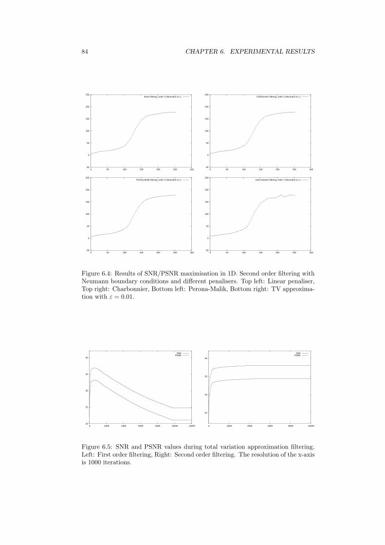
84 CHAPTER 6. EXPERIMENTAL RESULTS
-50
0
50
100
150
200
250
0 50 100 150 200 250 300
linear filtering, order 2 (Neumann b.c.)
-50
0
50
100
150
200
250
0 50 100 150 200 250 300
Charbonnier filtering, order 2 (Neumann b.c.)
-50
0
50
100
150
200
250
0 50 100 150 200 250 300
Perona-Malik filtering, order 2 (Neumann b.c.)
-50
0
50
100
150
200
250
0 50 100 150 200 250 300
total variation filtering, order 2 (Neumann b.c.)
Figure 6.4: Results of SNR/PSNR maximisation in 1D. Second order filtering withNeumann boundary conditions and different penalisers. Top left: Linear penaliser,Top right: Charbonnier, Bottom left: Perona-Malik, Bottom right: TV approxima-tion with ε = 0.01.
20
25
30
35
40
0 2000 4000 6000 8000 10000 12000
SNRPSNR
25
30
35
40
0 2000 4000 6000 8000 10000
SNRPSNR
Figure 6.5: SNR and PSNR values during total variation approximation filtering.Left: First order filtering, Right: Second order filtering. The resolution of the x-axisis 1000 iterations.

6.1. FILTERING RESULTS 85
-40
-20
0
20
40
0 50 100 150 200 250 300
Original signal
-40
-20
0
20
40
0 50 100 150 200 250 300
With Gaussian noise, standard deviation 10.0
Figure 6.6: Piecewise polynomial test signal. Left: Original signal. Right: Signalwith additive Gaussian noise, standard deviation 10.0.
-40
-20
0
20
40
0 50 100 150 200 250 300
total variation filtering, order 1
-40
-20
0
20
40
0 50 100 150 200 250 300
total variation filtering, order 2, natural b.c.
-40
-20
0
20
40
0 50 100 150 200 250 300
total variation filtering, order 3, natural b.c.
-40
-20
0
20
40
0 50 100 150 200 250 300
total variation filtering, order 4, natural b.c.
Figure 6.7: Results of SNR/PSNR maximisation with total variation approxima-tions, ε = 10−2, and natural boundary conditions. Top left: Order 1, Top right:Order 2, Bottom left: Order 3, Bottom right: Order 4.

86 CHAPTER 6. EXPERIMENTAL RESULTS
Order Bound. Cond. τ SNR PSNR Iterations1 Neumann 5 · 10−5 15.92 19.70 3.93 · 105
2 Neumann 1.25 · 10−5 17.94 21.72 8.30 · 106
2 Natural 1.25 · 10−5 17.98 21.76 1.32 · 107
3 Neumann 3.125 · 10−6 17.97 21.75 6.59 · 107
3 Natural 3.125 · 10−6 18.11 21.89 1.08 · 108
4 Neumann 7.8125 · 10−7 17.79 21.57 7.62 · 108
4 Natural 7.8125 · 10−7 > 17.56 > 21.33 > 2.7 · 109
Table 6.6: SNR/PSNR values for total variation approximation with ε = 10−4 andthe piecewise polynomial signal.
-2
-1.5
-1
-0.5
0
0.5
1
1.5
2
0 50 100 150 200 250 300
epsilon = 0.01epsilon = 0.0001
-0.2
-0.15
-0.1
-0.05
0
0.05
0.1
0.15
0.2
0 50 100 150 200 250 300
epsilon = 0.01epsilon = 0.0001
Figure 6.8: Derivative approximations for filtering results. Left: First derivative ofsecond order filtering result. Right: Second derivative of third order filtering result.
109 iterations due to the high running time (the SNR and PSNR values were stillincreasing at that moment).
We see that in terms of SNR and PSNR, the differences between both filteringmethods for ε are not very big. The filtering results also look very similar, thuswe have only shown the results for ε = 10−2 in Figure 6.7. As a technical remarkwe should add that the small time step sizes for filtering of third and fourth order(especially with ε = 10−4) demand relatively high calculation precision. For theimplementations in C we had to use the floating point data type double instead offloat for the higher order examples.
For a further understanding of the differences between the two cases we havea look at the derivative approximations of the filtering results. The conjecturethat mth order total variation approximation filtering yields results that piecewiseconsist of polynomials of degree m − 1 has already been mentioned. The filteringresults in Figure 6.7 seem to confirm this hypothesis.
To obtain further indications we consider the finite difference approximation ofthe (m − 1)th derivative for the results of mth order filtering. To corroborate ourbelief this (m− 1)th derivative should be piecewise constant. Figure 6.8 shows thatthe behaviour of the derivative strongly depends on the value of ε. For ε = 10−4
the derivative approximations really seem to be piecewise constant. Though theyare not shown here similar results can also be found for fourth order filtering andthe third derivative.
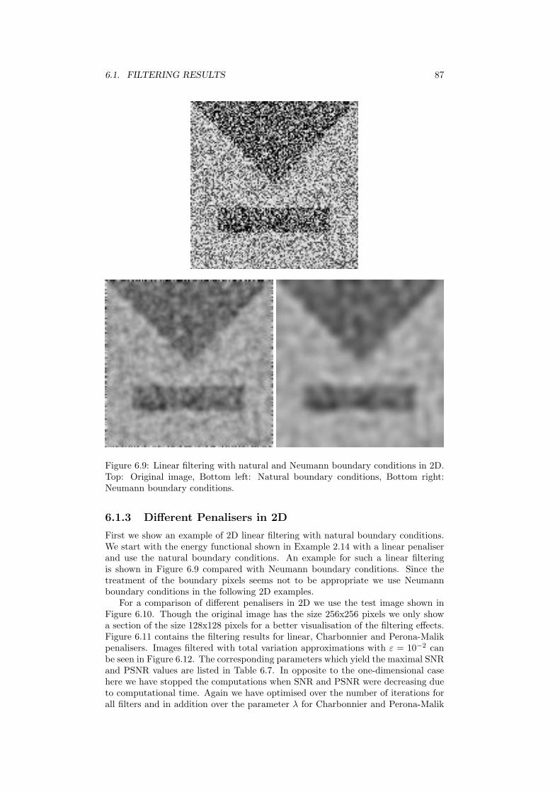
6.1. FILTERING RESULTS 87
Figure 6.9: Linear filtering with natural and Neumann boundary conditions in 2D.Top: Original image, Bottom left: Natural boundary conditions, Bottom right:Neumann boundary conditions.
6.1.3 Different Penalisers in 2D
First we show an example of 2D linear filtering with natural boundary conditions.We start with the energy functional shown in Example 2.14 with a linear penaliserand use the natural boundary conditions. An example for such a linear filteringis shown in Figure 6.9 compared with Neumann boundary conditions. Since thetreatment of the boundary pixels seems not to be appropriate we use Neumannboundary conditions in the following 2D examples.
For a comparison of different penalisers in 2D we use the test image shown inFigure 6.10. Though the original image has the size 256x256 pixels we only showa section of the size 128x128 pixels for a better visualisation of the filtering effects.Figure 6.11 contains the filtering results for linear, Charbonnier and Perona-Malikpenalisers. Images filtered with total variation approximations with ε = 10−2 canbe seen in Figure 6.12. The corresponding parameters which yield the maximal SNRand PSNR values are listed in Table 6.7. In opposite to the one-dimensional casehere we have stopped the computations when SNR and PSNR were decreasing dueto computational time. Again we have optimised over the number of iterations forall filters and in addition over the parameter λ for Charbonnier and Perona-Malik
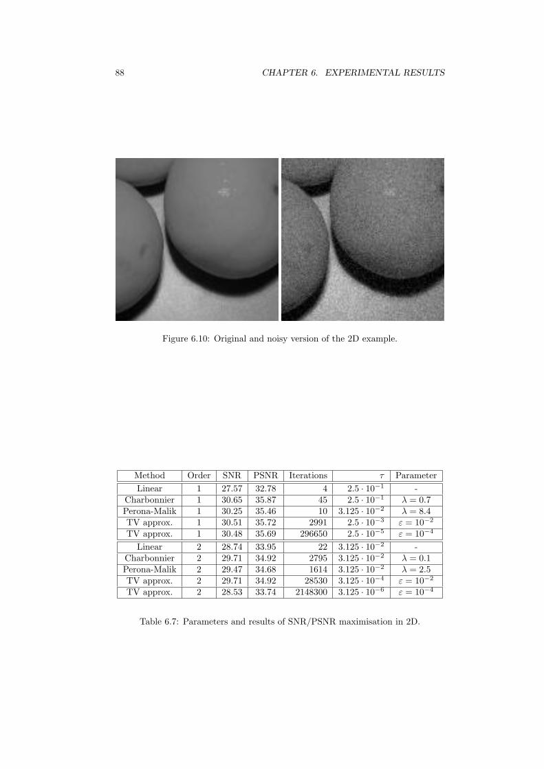
88 CHAPTER 6. EXPERIMENTAL RESULTS
Figure 6.10: Original and noisy version of the 2D example.
Method Order SNR PSNR Iterations τ ParameterLinear 1 27.57 32.78 4 2.5 · 10−1 -
Charbonnier 1 30.65 35.87 45 2.5 · 10−1 λ = 0.7Perona-Malik 1 30.25 35.46 10 3.125 · 10−2 λ = 8.4TV approx. 1 30.51 35.72 2991 2.5 · 10−3 ε = 10−2
TV approx. 1 30.48 35.69 296650 2.5 · 10−5 ε = 10−4
Linear 2 28.74 33.95 22 3.125 · 10−2 -Charbonnier 2 29.71 34.92 2795 3.125 · 10−2 λ = 0.1Perona-Malik 2 29.47 34.68 1614 3.125 · 10−2 λ = 2.5TV approx. 2 29.71 34.92 28530 3.125 · 10−4 ε = 10−2
TV approx. 2 28.53 33.74 2148300 3.125 · 10−6 ε = 10−4
Table 6.7: Parameters and results of SNR/PSNR maximisation in 2D.

6.1. FILTERING RESULTS 89
Figure 6.11: Results of SNR maximisation in 2D. Left column: First order filtering,Right column: Second order filtering with Neumann boundary conditions. Firstrow: Linear penaliser, Second row: Charbonnier penaliser, Third row: Perona-Malik penaliser.

90 CHAPTER 6. EXPERIMENTAL RESULTS
Figure 6.12: Results of SNR maximisation in 2D, Total variation approximationwith ε = 10−2. Left column: First order filtering, Right column: Second orderfiltering with Neumann boundary conditions.
filters. We see that in this case the SNR and PSNR of second order filtering are abit smaller than the ones for first order filtering.
One can state that the second order filtering results seem to contain isolatedwhite or black pixels or speckle artifacts near edges. Similar observations are men-tioned in [34] where an algorithm based on mean and variance in a neighbourhoodfor the removal of these artifacts is proposed. This would require a postprocessingstep after the filtering to remove the speckle artifacts. In Section 6.3 we will give anindication that it could be possible to avoid these artifacts within the higher orderfiltering framework.
6.2 Different Discretisation Methods
In this section we give an example for the comparison of different filter implemen-tations. We compare explicit schemes for Perona-Malik filtering of order 2 withNeumann boundary conditions. To discretise the Laplacian we use the matricesL (which will be called Laplacian 1) and L (Laplacian 2) from Section 4.2.4 andthe matrix DS from Section 4.3.3. All three filters were started with the sameparameters (step size, number of iterations and λ) to get comparable conditions.Figure 6.2 shows the filtering results for all three filters and the pairwise differencesbetween them. Here we take the complete 256x256 pixels of our test image. Theimage values were rounded and truncated to values from 0 to 255 before takingthe differences. For better visualisation the grey values of the difference imageswere linearly rescaled to the range 0 to 255. To give a quantitative impression thefollowing table contains the minimum, maximum, mean and standard deviation ofthe difference images before they were rescaled.
Min Max Mean Standard deviationL1 and L2 0.0 18.0 0.2 0.65L1 and S 0.0 24.0 2.0 1.6L2 and S 0.0 26.0 2.0 1.7
With a mean of up to 2.0 the differences can be considered as rather small. For prac-tical purposes this could be interesting since spectral methods require two Fourier

6.2. DIFFERENT DISCRETISATION METHODS 91
Figure 6.13: Left column: Filtering results. Top left: Laplace 1, Middle left: Laplace2, Bottom left: Spectral methods. Right column: Differences. Top right: Laplace 1vs. Laplace 2, Middle right: Laplace 1 vs. Spectral methods, Bottom right: Laplace2 vs. Spectral methods.

92 CHAPTER 6. EXPERIMENTAL RESULTS
transforms in each step. The complexity is then O(n log n) if the Fast Fourier Trans-form can be used or O(n2) for the regular Discrete Fourier Transform. For finitedifference methods one step has complexity O(n) since for each pixel at most aneighbourhood of fixed size has to be considered. If the qualitative differences arenot very large, one would prefer the finite difference implementations because theyare faster than the spectral methods when an explicit time discretisation is usedand the problem is nonlinear. The difference image on the right-hand side of Figure6.2 shows where the greatest differences appear. We note that the influence of thediscretisation methods gets higher near edges of the image.
6.3 Combinations of Different Orders
To conclude this chapter we show some examples of filtering processes of combinedfirst and second order. A nonlinear energy functional in 1D for these filters waspresented in Example 2.11. For our filtering example we have used a convex com-bination of the smoothness terms of first and second order in 2D:
E(u) =∫Ω
((u− f)2 + α
((1− β)ϕ1
(|∇u|2
)+ βϕ2
((∆u)2
)))dz.
The corresponding diffusion equation in 2D is
ut = (1− β)div(ϕ′1(|∇u|2
)∇u)− β∆
(ϕ′2
((∆u)2
)∆u)
u(·, 0) = f
with stopping time α and β ∈ [0, 1].Figure 6.14 shows some filtering tests with a combination of first and second
order Perona-Malik filtering. So we are using the diffusivities
ϕ′k(x) =1
1 + xλ2
k
k = 1, 2
in the above equation. The example was obtained using the paramters β = 0.5, λ1 =5.0, and λ2 = 1.0. The images have size 256x256 pixels. We show here a section ofsize 128x128 pixels.
The first order filter produces stair-casing in the background while in the secondorder example the edges contain a lot of speckle artifacts. The combined methodreduces both shortcomings without a postprocessing step. We should add thatthe above results are not optimised with respect to SNR or PSNR. With such anoptimisation each of the methods also could lead to better results. This exam-ple indicates that the combination of different filter orders could possibly improvefiltering results.

6.3. COMBINATIONS OF DIFFERENT ORDERS 93
Figure 6.14: Top left: Noisy input image, Top right: First order Perona-Malik,Bottom left: Second order Perona-Malik, Bottom right: Combined filter with firstand second order.

94 CHAPTER 6. EXPERIMENTAL RESULTS

Chapter 7
Summary and Outlook
In this thesis we have considered higher order methods for signal and image restora-tion. We now summarise the main results and point out some open questions anddirections for further work.
In Chapter 2 we have discussed necessary and sufficient conditions for minimis-ers of energy functionals. Here an image is represented by a real-valued functiondepending on one or two real variables. That means we considered only grey valueimages. We have developed the Euler-Lagrange equations with the natural bound-ary conditions for one- and two-dimensional energy functionals.
After investigating energy functionals and corresponding necessary conditionsfor a minimiser we have turned our attention to strategies how to use these condi-tions to obtain such a minimiser. In Chapter 3 we considered this filtering processin the framework of continuous functions. For higher order filtering with linear pe-nalisers we oriented at [18]. We discussed also some scale-space properties of linearfiltering using higher order linear diffusion equations. Analogously to first order fil-tering we introduced some well-posedness considerations for nonlinear second orderequations of diffusion type. As applications we studied the behaviour for differentpenalisers. We found out that linear, Charbonnier and total variation approxima-tions always perform forward diffusion. Total variation is the border case betweenforward and backward diffusion while the Perona-Malik penaliser can perform bothforward and backward diffusion and can therefore be ill-posed.
The discrete part of the work started with giving different ways for derivativeapproximation with finite differences and spectral methods. Our special interestwas on natural and Neumann boundary conditions. We derived matrix notationsfor finite difference and spectral derivative approximations in one dimension witharbitrary derivative order and both types of boundary conditions. We investigatedthe properties of these matrices in terms of spectral norm and kernel.
We concluded the theoretical part with Chapter 5 by giving discretisations ofthe approaches in Chapter 3 that were used in concrete algorithms. The semi-discrete case for the corresponding diffusion equations was also investigated. Wehave derived that one-dimensional finite difference methods with natural boundaryconditions yield least-square polynomial data fittings for t −→ ∞ while Neumannboundary conditions lead to the average grey value. Then the main focus was onexplicit discretisations of the corresponding diffusion equations. Stability limits forthe time step size τ were derived for different derivative orders and approximations.The results of our numerical tests were presented in Chapter 6.
We can conclude that the presented methods seem to produce really betterresults for signal processing. Besides the optical impression also the SNR andPSNR results are clearly better for higher order methods. Especially the totalvariations approximations fit in the imagination of yielding piecewise polynomial
95

96 CHAPTER 7. SUMMARY AND OUTLOOK
signals. The second order seems to be a compromise between avoiding stair-casingand too high adaption at the noise. The image processing examples with secondorder filtering often suffer from artifacts around edges. Our numerical tests suggestthat combined methods with first and second order derivatives could reduce or evencompletely avoid this shortcoming. It also seems to be possible to choose parameterssets such that combined methods of first and second order satisfy a minimum-maximum property. If this observation could be mathematically confirmed thecombined nonlinear methods of first and second order would yield a compromisewhich avoids the stair-casing of first order methods and the edge artifacts of secondorder methods.
After this short summary of the main results we consider some open questionswhich invite us to further studies: In real world applications multi-channel imageswith values in Rn appear in a natural way. An obvious generalisation for colourimages requires the theory for images with values in R3, for example. One mayalso think of medical data like NMR images which are matrix-valued. The imagesmay also depend on more than two variables. For such applications the resultspresented in Chapter 2 have to be extended. For functionals depending only onthe first derivatives these extensions are covered in [9]. For higher derivatives thisshould also be possible without great changes in the reasoning.
For our numerical tests we only used explicit schemes. To make the methodspractically useful other algorithms have to be applied which reduce the runningtime. With implicit schemes for example higher values for the temporal step size τcould be chosen and the number of iterations would become smaller.
The properties of the combined filters of first and second order are anotherinteresting point. In particular the existence of conditions for a maximum-minimumproperty of these filters seems to be possible.
We should also mention that all methods presented in this work are isotropic.It would be interesting to investigate how higher order anisotropic filters wouldbehave. In the first order case a description of anisotropic filters can be found in[31]. In the higher order framework one may think of second order diffusion alongthe eigenvectors of the Hessian. Perhaps one could implement coherence-enhancingor edge-enhancing filters similar to the first order case.

Bibliography
[1] R. Acar and C. R. Vogel. Analysis of bounded variation penalty methods forill-posed problems. Inverse Problems, 10:1217–1229, 1994.
[2] A. M. Arthurs. Calculus of Variations. Routledge & Kegan Paul Ltd., 1975.
[3] M. Bertero, T. A. Poggio, and V. Torre. Ill-posed problems in early vision.Proc. IEEE, 76:869–889, 1988.
[4] G. Boole. Calculus of Finite Differences. Chelsea Publishing Company, fourthedition, 1872.
[5] T. Chan, A. Marquina, and P. Mulet. High-order total variation-based imagerestoration. SIAM Journal of Scientific Computing, 22(2):503–516, 2000.
[6] P. Charbonnier, L. Blanc-Feraud, G. Aubert, and M. Barlaud. Two deter-ministic half-quadratic regularization algorithms for computed imaging. Proc.IEEE International Conference on Image Processing (ICIP-94, Austin, Now.13-16, 1994), 2:168–172, 1994.
[7] G. Fischer. Lineare Algebra. Vieweg Verlag, eleventh edition, 1997.
[8] I. M. Gelfand and S. V. Fomin. Calculus of Variations. Prentice-Hall, Inc.,Englewood Cliffs, New Jersey, revised english edition, 1963.
[9] M. Giaquinta and S. Hildebrandt. Calculus of Variations I – The LagrangianFormalism. Springer-Verlag, 1996.
[10] J. B. Greer and A. L. Bertozzi. H1 solutions of a class of fourth order nonlinearequations for image processing. Discrete and Continuous Dynamical Systems,10(1 and 2), January and March 2004.
[11] C. Grossmann and H.-G. Roos. Numerik partieller Differentialgleichungen.B. G. Teubner Stuttgart, second edition, 1994.
[12] H. Heuser. Gewohnliche Differentialgleichungen – Einfuhrung in Lehre undGebrauch. B. G. Teubner Stuttgart, second edition, 1991.
[13] H. Heuser. Funktionalanalysis – Theorie und Anwendung. B. G. TeubnerStuttgart, third edition, 1992.
[14] F. B. Hildebrand. Finite-Difference Equations and Simulations. Prentice-HallInc., Englewood Cliffs, New Jersey, 1968.
[15] R. A. Horn and C. A. Johnson. Matrix Analysis. Cambridge University Press,1985.
[16] T. Iijima. Theory of pattern recognition. Electronics and Communications inJapan, pages 123–124, 1963.
97
98 BIBLIOGRAPHY
[17] M. Lysaker, A. Lundervold, and X.-C. Tai. Noise removal using fourth-orderpartial differential equations with applications to medical magnetic resonanceimages in space and time. Technical report, University of California, Los An-geles, Juli 2002.
[18] M. Nielsen, L. Florack, and R. Deriche. Regularization, scale-space and edgedetection filters. Journal of Mathematical Imaging and Vision, 7:291–307, 1997.
[19] N. Nordstrom. Biased anisotropic diffusion – a unified regularization and dif-fusion approach to edge detection. Image and Vision Computing, 8:318–327,1990.
[20] P. Perona and J. Malik. Scale space and edge detection using anisotropicdiffusion. IEEE Trans. Pattern Anal. Mach. Intell., 12:629–639, 1990.
[21] L. I. Rudin, S. Osher, and E. Fatemi. Nonlinear total variation based noiseremoval algorithms. Physica D, 60:259–268, 1992.
[22] O. Scherzer and J. Weickert. Relations between regularization and diffusionfiltering. Journal of Mathematical Imaging and Vision, 12:43–63, 2000.
[23] C. Schnorr. Unique reconstruction of piecewise smooth images by minimizingstrictly convex non-quadratic functionals. Journal of Mathematical Imagingand Vision, 4:189–198, 1994.
[24] H. R. Schwarz. Numerische Mathematik. B. G. Teubner Stuttgart, 1997.
[25] G. D. Smith. Numerical Solution of Partial Differential Equations: FiniteDifference Methods. Clarendon Press, Oxford, 1978.
[26] J. Stoer and R. Bulirsch. Introduction to Numerical Analysis. Springer-VerlagNew York, Inc., third edition, 2002.
[27] M. E. Taylor. Partial Differential Equations I. Springer-Verlag New York, Inc.,1996.
[28] A. N. Tikhonov. Solution of incorrectly formulated problems and the regular-ization method. Soviet Mathematics Doklady, 4(2):1035–1038, 1963.
[29] L. N. Trefethen. Finite Difference and Spectral Methods for Ordinary andPartial Differential Equations. Unpublished, 1996. Available at the URLhttp://web.comlab.ox.ac.uk/oucl/work/nick.trefethen/pdetext.html.
[30] W. Walter. Analysis 2. Springer-Verlag Berlin Heidelberg, fourth edition, 1995.
[31] J. Weickert. Anisotropic Diffusion in Image Processing. B. G. TeubnerStuttgart, 1998.
[32] J. Weickert, S. Ishikawa, and A. Imiya. Linear scale-space has first been pro-posed in Japan. Journal of Mathematical Imaging and Vision, 10:237–252,1999.
[33] D. Werner. Funktionalanalysis. Springer-Verlag Berlin Heidelberg, third edi-tion, 2000.
[34] Y.-L. You and M. Kaveh. Fourth-order partial differential equations for noiseremoval. IEEE Transactions on Image Processing, 9(10):1723–1730, October2000.
[35] F. Zhang. Matrix Theory – Basic Results and Techniques. Springer-VerlagNew York, Inc., 1999.