dependence analysis via copulas - ime.usp.brjmsinger/mae5705/kolev2015.pdf · nikolai kolev,...
TRANSCRIPT
IntroductionCopula basics
Dependence measuresCopula families
Estimation and model fittingReal data analysis: Option pricing via Copulas
Dependence Analysis via Copulas
Nikolai Kolev, Leandro Ferreira and Rafael Aguilera
IME-USP
Contact e-mails: [email protected]
[email protected] and [email protected]
c© Kolev & PFA
Nikolai Kolev, Leandro Ferreira and Rafael Aguilera Dependence Analysis via Copulas

IntroductionCopula basics
Dependence measuresCopula families
Estimation and model fittingReal data analysis: Option pricing via Copulas
Outline
Introduction
Copula: Definition, Sklar’s Theorem, Examples, Simulation
Dependence Measures
Copula Families
Estimation and Model Fitting
Real data analysis: Option pricing via Copulas
Nikolai Kolev, Leandro Ferreira and Rafael Aguilera Dependence Analysis via Copulas

IntroductionCopula basics
Dependence measuresCopula families
Estimation and model fittingReal data analysis: Option pricing via Copulas
Continuous univariate distributions
Let X be a continuous random variable with distribution F (x) = P(X ≤ x).
1 F (x) is non-decreasing;
2 Inverse function is given by F−1(u) = infx∈<{F (x) ≥ u}, u ∈ [0, 1], which
is non-decreasing as well;
Density function: f (x) = ddxF (x).
1 f (x) ≥ 0 such that∫∞−∞ f (u) du = 1;
2 F (x) =∫ x
−∞ f (u) du;
3 P(a < X ≤ b) =∫ b
af (u) du = F (b)− F (a).
Nikolai Kolev, Leandro Ferreira and Rafael Aguilera Dependence Analysis via Copulas
IntroductionCopula basics
Dependence measuresCopula families
Estimation and model fittingReal data analysis: Option pricing via Copulas
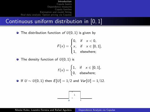
Continuous uniform distribution in [0, 1]
The distribution function of U(0, 1) is given by
F (x) =
0, if x < 0,
x , if x ∈ [0, 1],
1, elsewhere;
The density function of U(0, 1) is
f (x) =
{1, if x ∈ [0, 1],
0, elsewhere;
If U ∼ U(0, 1) then E [U] = 1/2 and Var [U] = 1/12.
Nikolai Kolev, Leandro Ferreira and Rafael Aguilera Dependence Analysis via Copulas

IntroductionCopula basics
Dependence measuresCopula families
Estimation and model fittingReal data analysis: Option pricing via Copulas
Probability integral transform 1
Let X be a continuous random variable with distributionfunction F (x). The relation U = F (X ) is denominatedprobability integral transform.
The distribution function of random variable U = F (X ) is
P(F (X ) ≤ u) = P(X ≤ F−1(u)) = F (F−1(u)) = u.
Thus, Ud= F (X ) ∼ U(0, 1) ⇔ F−1(U)
d= X .
Therefore, random variables F−1(U) and X share the samedistribution.
Nikolai Kolev, Leandro Ferreira and Rafael Aguilera Dependence Analysis via Copulas
IntroductionCopula basics
Dependence measuresCopula families
Estimation and model fittingReal data analysis: Option pricing via Copulas
Probability integral transform 2
Probability integral transform
Given a continuouis random variable X with distribution functionF (x), the random variable U = F (X ) ∼ U(0, 1). Moreover,
Xd= F−1(U) ∼ F (x).
This result is useful for simulating continuous random variableswith known distribution function F (x) using the standarduniform random numbers generator.
Nikolai Kolev, Leandro Ferreira and Rafael Aguilera Dependence Analysis via Copulas

IntroductionCopula basics
Dependence measuresCopula families
Estimation and model fittingReal data analysis: Option pricing via Copulas
”Discrete” probability integral transform
Let X be a discrete random variable defined by pi = P(X = xi ) ≥ 0,∑
pi = 1,then F (X ) is not U(0, 1)-distributed.
In fact, if X is given by
X x1 x2 x3 · · ·Prob. p1 p2 p3 · · ·
with distribution function F (x) = P(X ≤ x) =∑
j≤i pj , for xi ≤ x < xi+1. Then
Y = F (X ) is discrete random variable
Y = F (X ) p1 p1 + p2 p1 + p2 + p3 · · ·Prob. p1 p2 p3 · · ·
which is not U(0, 1), but
E [F (X )] = 1/2 + 1/2k∑
i=1
p2i
k→∞−−−−→ 1/2 which is the mean of U(0, 1),
Var [F (X )] = 1/12 + f
(k∑
i=1
p2i
)k→∞−−−−→ 1/12 which is the variance of U(0, 1)
Nikolai Kolev, Leandro Ferreira and Rafael Aguilera Dependence Analysis via Copulas
IntroductionCopula basics
Dependence measuresCopula families
Estimation and model fittingReal data analysis: Option pricing via Copulas
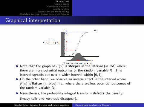
Graphical interpretation
Note that the graph of F (x) is steeper in the interval (in red) wherethere are more potential outcomes of the random variable X . Thisinterval spreads out over a wider interval within [0, 1];On the other hand, we observe an inverse effect in the interval whereF (x) is flatter (in blue), i.e., where there are less potential outcomes ofthe random variable X ;
Nevertheless, the probability integral transform defects the density
(heavy tails and kurthosis disappear).
Nikolai Kolev, Leandro Ferreira and Rafael Aguilera Dependence Analysis via Copulas

IntroductionCopula basics
Dependence measuresCopula families
Estimation and model fittingReal data analysis: Option pricing via Copulas
Simulating a logistic distribution
If X follows a logistic distribution with parameters β ≥ 0and µ ∈ < = (−∞,∞), its distribution function is given by
F (x) =1
1 + exp(− x−µβ )
, x ∈ < = (−∞,∞);
The inverse F−1(·) of F can be found as a solution of
u = F (x)⇒ x = F−1(u) = µ− β ln(u−1 − 1);
Simulating logistic distribution with parameters β and µ:1 Using a standard uniform random numbers generator, generate
u ∈ [0, 1];2 Calculate x = F−1(u) = µ− β ln(u−1 − 1), which is the
required observation (since Xd= F−1(U)).
Nikolai Kolev, Leandro Ferreira and Rafael Aguilera Dependence Analysis via Copulas

IntroductionCopula basics
Dependence measuresCopula families
Estimation and model fittingReal data analysis: Option pricing via Copulas
Commands in R
We will simulate a sample with size N = 10000 of a logisticdistribution with parameters µ = β = 2.
The commands in R are:
1 # S i m u l a t i o n o f a l o g i s t i c d i s t r i b u t i o n23 N = 100004 U = r u n i f (N)5 mi = 26 b e t a = 27 X = mi−b e t a∗ l o g ( ( 1 /U)−1)8 h i s t (X, 3 0 , f r e q=FALSE , main=”” )
Nikolai Kolev, Leandro Ferreira and Rafael Aguilera Dependence Analysis via Copulas

IntroductionCopula basics
Dependence measuresCopula families
Estimation and model fittingReal data analysis: Option pricing via Copulas
Histogram of logistic distribution (µ = β = 2)
Nikolai Kolev, Leandro Ferreira and Rafael Aguilera Dependence Analysis via Copulas

IntroductionCopula basics
Dependence measuresCopula families
Estimation and model fittingReal data analysis: Option pricing via Copulas
Continuous bivariate distributions
Joint distribution of (X ,Y ): H(x , y) = P(X ≤ x ,Y ≤ y);
Marginal distributions:
F (x) = limy→∞
H(x , y) and G (y) = limx→∞
H(x , y);
Density function: h(x , y) = ∂2
∂x∂yH(x , y) ≥ 0, satisfying∫∞u=−∞
∫∞v=−∞ h(u, v)dudv = 1;
Marginal density functions: f (x) =∫∞−∞ h(x , u)du = d
dx F (x)
and g(y) =∫∞−∞ h(u, y)du = d
dyG (y).
Nikolai Kolev, Leandro Ferreira and Rafael Aguilera Dependence Analysis via Copulas

IntroductionCopula basics
Dependence measuresCopula families
Estimation and model fittingReal data analysis: Option pricing via Copulas
Copula: definition and Sklar’s Theorem
Definition (Bivariate copula)
A bivariate copula is a bivariate distribution function C : [0, 1]2 → [0, 1], withstandard uniform marginal distributions, i.e., C(u, v) = P(U ≤ u,V ≤ v),where U and V ∼ U(0, 1).Therefore, C(u, v) is non-decreasing in itsarguments; C(0, 0) = 0; C(1, 1) = 1.
Sklar’s Theorem (Sklar, 1959)
Let H(x , y) be a bivariate distribution function with marginal distributionsF (x) and G(y). Then there exists a copula C : [0, 1]2 → [0, 1] such that
H(x , y) = C(F (x),G(y)),
for all (x , y) ∈ [−∞,∞]2. If F (x) and G(y) are continuous, then C is unique;otherwise, C is uniquely determined on RanX × RanY .
Nikolai Kolev, Leandro Ferreira and Rafael Aguilera Dependence Analysis via Copulas

IntroductionCopula basics
Dependence measuresCopula families
Estimation and model fittingReal data analysis: Option pricing via Copulas
Obtaining the copula C (u, v) from H(x , y)
From relations F (x) = u and G (y) = v , where u, v ∈ [0, 1],we obtain x = F−1(u) and y = G−1(v).
Substituting x = F−1(u) and y = G−1(v) inH(x , y) = C (F (x),G (y)), we get the copula C (u, v).
Obtaining copula C (u, v) from joint distribution H(x , y)
Given a bivariate distribution function H(x , y), the correspondingcopula is
C (u, v) = H(F−1(u),G−1(v)
),
for all (u, v) ∈ [0, 1]2.
Nikolai Kolev, Leandro Ferreira and Rafael Aguilera Dependence Analysis via Copulas

IntroductionCopula basics
Dependence measuresCopula families
Estimation and model fittingReal data analysis: Option pricing via Copulas
Graphical interpretation 1
H(x , y) = P(X ≤ x ,Y ≤ y) H(x , y) = C (F (x),G (y))
F (x) = P(X ≤ x), G (y) = P(Y ≤ y) C (u, v) = H(F−1(u),G−1(v))
Ud= F (X ) ∼ U(0, 1), V
d= G (Y ) ∼ U(0, 1)
Nikolai Kolev, Leandro Ferreira and Rafael Aguilera Dependence Analysis via Copulas

IntroductionCopula basics
Dependence measuresCopula families
Estimation and model fittingReal data analysis: Option pricing via Copulas
Graphical interpretation 1
Starting from the joint density h(x , y) we can obtain the marginaldensities by f (x) =
∫∞−∞ h(x , u)du and g(y) =
∫∞−∞ h(u, y)du.
Nikolai Kolev, Leandro Ferreira and Rafael Aguilera Dependence Analysis via Copulas

IntroductionCopula basics
Dependence measuresCopula families
Estimation and model fittingReal data analysis: Option pricing via Copulas
Graphical interpretation 1
The marginal distribution functions are given by F (x) =∫ x
−∞ f (u) du and
G(y) =∫ y
−∞ g (v) dv .
Nikolai Kolev, Leandro Ferreira and Rafael Aguilera Dependence Analysis via Copulas

IntroductionCopula basics
Dependence measuresCopula families
Estimation and model fittingReal data analysis: Option pricing via Copulas
Graphical interpretation 1
From the marginal distributions we have U = F (X ) and V = G(Y ),which are uniformly distributed in [0, 1].
Nikolai Kolev, Leandro Ferreira and Rafael Aguilera Dependence Analysis via Copulas

IntroductionCopula basics
Dependence measuresCopula families
Estimation and model fittingReal data analysis: Option pricing via Copulas
Graphical interpretation 1
The joint distribution of (U,V ) is copula C(u, v) = P(U ≤ u,V ≤ v).
Nikolai Kolev, Leandro Ferreira and Rafael Aguilera Dependence Analysis via Copulas

IntroductionCopula basics
Dependence measuresCopula families
Estimation and model fittingReal data analysis: Option pricing via Copulas
Graphical interpretation 1
Nikolai Kolev, Leandro Ferreira and Rafael Aguilera Dependence Analysis via Copulas

IntroductionCopula basics
Dependence measuresCopula families
Estimation and model fittingReal data analysis: Option pricing via Copulas
Several reliable R Packages for Copulas
Package Title
copula Multivariate dependence with copulacopulaedas Estimation of distribution, Algorithms based on copulasCDVine Statistical inference of C- and D-vine copulasqcmr Gaussian copula marginal regressionnacopula Nested Archimedean copulasqrm Quantitative risk managment
Nikolai Kolev, Leandro Ferreira and Rafael Aguilera Dependence Analysis via Copulas

IntroductionCopula basics
Dependence measuresCopula families
Estimation and model fittingReal data analysis: Option pricing via Copulas
Graphical interpretation 2: Commands in R
Generating a sample of size 10000 of:
a bivariate normal distribution H(x , y) with standard normal N(0, 1)marginals and correlation coefficient ρ has density
φ2,ρ(x , y) =1
2π√
1− ρ2exp
(− 1
2(1− ρ2)[x2 + y2 − 2ρxy ]
);
corresponding copula C (u, v) via Sklar’s theorem with ρ = 0.7.
1 l i b r a r y ( mvtnorm )2 #Step 1 : G e n e r a t i n g a sample from H3 c1<−c ( 1 , . 7 ) ; c2<−c ( . 7 , 1 ) ; R=c b i n d ( c1 , c2 )4 sample <− rmvnorm ( n=10000 , mean=c ( 0 , 0 ) , s igma=R)5 p l o t ( sample [ , 1 ] , sample [ , 2 ] , x l a b=” x ” , y l a b=” y ” , pch=” . ” , cex =1.5 , main=” Sample from H
” )67 #Step 2 : G e n e r a t i n g a sample from C v i a S k l a r ’ s Theorem8 sample . c o p u l a=pnorm ( sample )9 p l o t ( sample . copu la , x l a b=”u” , y l a b=” v ” , pch=” . ” , cex =1.5 , main=” Sample from C” )
Nikolai Kolev, Leandro Ferreira and Rafael Aguilera Dependence Analysis via Copulas

IntroductionCopula basics
Dependence measuresCopula families
Estimation and model fittingReal data analysis: Option pricing via Copulas
Standard bivariate Normal distribution and its copula
Scatterplot of a sample of size 10000
Nikolai Kolev, Leandro Ferreira and Rafael Aguilera Dependence Analysis via Copulas

IntroductionCopula basics
Dependence measuresCopula families
Estimation and model fittingReal data analysis: Option pricing via Copulas
Comments
Copula contains all the information about the dependencestructure independent of marginal influence since
C (F (x),G (y)) = H(x , y);
Copulas enable us to model marginal distributions and thedependence structure separately;
Copulas provide modelling flexibility: given a copula we canobtain many multivariate distributions by selecting differentmarginal distributions;
Any bivariate distribution can be used to construct a copula:C (u, v) = H
(F−1(u),G−1(v)
).
Nikolai Kolev, Leandro Ferreira and Rafael Aguilera Dependence Analysis via Copulas

IntroductionCopula basics
Dependence measuresCopula families
Estimation and model fittingReal data analysis: Option pricing via Copulas
Example 1 - symmetric bivariate Gumbel distribution
Symmetric (H(x , y) = H(y , x)) bivariate Gumbel distribution
H(x , y) = [1 + exp (−x) + exp (−y)]−1 ,
for all x , y ∈ [−∞,+∞] ;
The marginal distribution of X isF (x) = lim
y→∞H(x , y) = [1 + exp(−x)]−1;
The inverse F−1(u) is the solution of u = F (x), i.e.
F (x) = [1 + exp(−x)]−1 = u ⇒ exp(−x) =1
u− 1 =
1− u
u.
and therefore,
x = − ln
(1− u
u
)= F−1(u).
Nikolai Kolev, Leandro Ferreira and Rafael Aguilera Dependence Analysis via Copulas

IntroductionCopula basics
Dependence measuresCopula families
Estimation and model fittingReal data analysis: Option pricing via Copulas
Example 1 - copula of bivariate Gumbel distribution
By analogy, y = − ln(
1−vv
)= G−1(v);
In H(x , y) = [1 + exp (−x) + exp (−y)]−1 we substitutex = F−1(u) and y = G−1(v) to get
C (u, v) = H(F−1(u),G−1(v)
)={
1 + exp[ln( 1−u
u )]
+ exp[ln( 1−v
v )])}−1;
Thus, the copula of bivariate symmetric Gumbel distribution is
C (u, v) =
{1 +
1− u
u+
1− v
v
}−1
=uv
u + v − uv.
Nikolai Kolev, Leandro Ferreira and Rafael Aguilera Dependence Analysis via Copulas

IntroductionCopula basics
Dependence measuresCopula families
Estimation and model fittingReal data analysis: Option pricing via Copulas
Example 1 - Graphs of bivariate Gumbel distribution
Bivariate Gumbel distribution and its copula
Scatterplot of a sample of size 10000
Nikolai Kolev, Leandro Ferreira and Rafael Aguilera Dependence Analysis via Copulas

IntroductionCopula basics
Dependence measuresCopula families
Estimation and model fittingReal data analysis: Option pricing via Copulas
Example 2 - copula of asymmetric distribution
Consider the asymmetric distribution (H(x , y) 6= H(y , x))
H(x , y) =
(x+1)[exp(y)−1]x+2 exp(y)−1 , if (x , y) ∈ [−1, 1]× [0,∞],
1− exp(−y), if (x , y) ∈ (1,∞)× [0,∞],
0, elsewhere.
(1)
The distribution function of the marginal variable X is
F (x) =
0, if x < −1,x+1
2 , if x ∈ [−1, 1],
1, elsewhere,
i.e., X ∼ U(−1, 1). Therefore, x = F−1(u) = 2u − 1.
Nikolai Kolev, Leandro Ferreira and Rafael Aguilera Dependence Analysis via Copulas
IntroductionCopula basics
Dependence measuresCopula families
Estimation and model fittingReal data analysis: Option pricing via Copulas
Example 2 - copula of asymmetric distribution
The distribution function of the random variable Y is
G (y) =
{0, if y < 0,
1− exp (−y) , elsewhere,
i.e., Y ∼ Exp (1) and y = G−1(v) = − ln(1− v);
Substituting solutions x = F−1(u) = 2u − 1 andy = G−1(v) = − ln(1− v) in H(x , y), given by (1), we obtain
C (u, v) =
{1 +
1− u
u+
1− v
v
}−1
=uv
u + v − uv.
Nikolai Kolev, Leandro Ferreira and Rafael Aguilera Dependence Analysis via Copulas

IntroductionCopula basics
Dependence measuresCopula families
Estimation and model fittingReal data analysis: Option pricing via Copulas
Conclusion: symmetric and asymmetric distributions withthe same copula, i.e. having the same dependencestructure ???
The symmetric bivariate Gumbel logistic distribution
H(x , y) = [1 + exp (−x) + exp (−y)]−1, for all x , y ∈ [−∞,+∞]
and the asymmetric distribution
H(x , y) =
(x+1)[exp(y)−1]x+2 exp(y)−1 , if (x , y) ∈ [−1, 1]× [0,∞],
1− exp(−y), if (x , y) ∈ (1,∞)× [0,∞],
0, elsewhere
share the same copula C (u, v) = H(F−1(u),G−1(v)) = uvu+v−uv ;
Mathematically correct, but confusing! Believe in to the same
dependence structure.
Nikolai Kolev, Leandro Ferreira and Rafael Aguilera Dependence Analysis via Copulas

IntroductionCopula basics
Dependence measuresCopula families
Estimation and model fittingReal data analysis: Option pricing via Copulas
Frechet-Hoeffding bounds for the joint distribution H(x , y)
The bounds for the distribution function H(x , y) are given by
max(F (x) + G (y)− 1, 0) ≤ H(x , y) ≤ min(F (x),G (y));
In absence of information about genuine dependence, thejoint distribution can be bounded by functions of marginals;
These bounds can also be written in terms of copulas as
max(u + v − 1, 0) ≤ C (u, v) ≤ min(u, v),
(use the relations F (x) = u, G (y) = v andC (u, v) = H(F−1(u),G−1(v)));
These bounds can be sharper under additional information(about the value of correlation coefficient, for example).
Nikolai Kolev, Leandro Ferreira and Rafael Aguilera Dependence Analysis via Copulas

IntroductionCopula basics
Dependence measuresCopula families
Estimation and model fittingReal data analysis: Option pricing via Copulas
Comonotonic copula M(u, v)
The upper Frechet-Hoeffding bound is the copulaM(u, v) = P(U ≤ u,V ≤ v) = min(u, v), i.e. U = V almostsurely and U and V are called comonotonic (meaning thatthey possess the highest possible positive dependence);The graph of the copula M(u, v) = min(u, v) is given below.
Nikolai Kolev, Leandro Ferreira and Rafael Aguilera Dependence Analysis via Copulas

IntroductionCopula basics
Dependence measuresCopula families
Estimation and model fittingReal data analysis: Option pricing via Copulas
Countermonotonic copula W (u, v)
The lower Frechet-Hoeffding bound is the copulaW (u, v) = P(U ≤ u,V ≤ v) = max(u + v − 1, 0);In this case, U = 1− V almost surely, and U and V arenamed countermonotonic, meaning that U and V exhibitthe extreme possible negative dependence;The graph of the copula W (u, v) = max(u + v − 1, 0) is givenbelow.
Nikolai Kolev, Leandro Ferreira and Rafael Aguilera Dependence Analysis via Copulas

IntroductionCopula basics
Dependence measuresCopula families
Estimation and model fittingReal data analysis: Option pricing via Copulas
Independent copula and level curves
The copula representing the independence structure betweenU and V is given byΠ(u, v) = P(U ≤ u,V ≤ v) = P(U ≤ u)P(V ≤ v) = uv ;
The independent copula Π(u, v) characterizes theindependence between U and V ;
Let H1(x , y) and H2(x , y) have the same marginaldistributions F (x) and G (y)
- If X and Y are independent, thenHi (x , y) = F (x)G (y), i=1,2 ;
- But the product F (x)G (y) does not characterizeindependence uniquelly.
Nikolai Kolev, Leandro Ferreira and Rafael Aguilera Dependence Analysis via Copulas
IntroductionCopula basics
Dependence measuresCopula families
Estimation and model fittingReal data analysis: Option pricing via Copulas
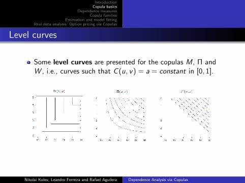
Level curves
Some level curves are presented for the copulas M, Π andW , i.e., curves such that C (u, v) = a = constant in [0, 1].
Nikolai Kolev, Leandro Ferreira and Rafael Aguilera Dependence Analysis via Copulas
IntroductionCopula basics
Dependence measuresCopula families
Estimation and model fittingReal data analysis: Option pricing via Copulas
Copula invariance under increasing transformation
Let X and Y be continuous random variables and let CXY (u, v) beits respective copula.
Copula invariance
If α(x) and β(y) are strictly increasing functions in DomX andDomY , then
Cα(X ),β(Y )(u, v) = CXY (u, v),
i.e., CXY (u, v) is invariant under strictly increasingtransformation of X and Y .
Nikolai Kolev, Leandro Ferreira and Rafael Aguilera Dependence Analysis via Copulas
IntroductionCopula basics
Dependence measuresCopula families
Estimation and model fittingReal data analysis: Option pricing via Copulas
Invariance proof
Proof.
Denote by F1, G1, F2 and G2 the distribution functions of X , Y ,α(X ) and β(Y ), respectively.Since α(x) and β(y) are strictly increasing functions,F2(x) = P[α(X ) ≤ x ] = P[X ≤ α−1(x)] = F1(α−1(x)).Analogously, G2(y) = G1(β−1(y)).Therefore, for all (x , y) in <2 we have
Cα(X ),β(Y )(F2(x),G2(y)) = P[α(X ) ≤ x , β(Y ) ≤ y ]= P[X ≤ α−1(x),Y ≤ β−1(y)]
= CXY (F1(α−1(x)),G1(β−1(y))) = CXY (F2(x),G2(y))
Since X and Y are continuous, DomF2 = DomG2 = [0, 1].Therefore, Cα(X ),β(Y )(u, v) = CX ,Y (u, v) in [0, 1]2.
Nikolai Kolev, Leandro Ferreira and Rafael Aguilera Dependence Analysis via Copulas
IntroductionCopula basics
Dependence measuresCopula families
Estimation and model fittingReal data analysis: Option pricing via Copulas
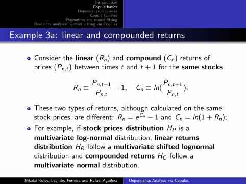
Example 3a: linear and compounded returns
Consider the linear (Rn) and compound (Cn) returns ofprices (Pn,t) between times t and t + 1 for the same stocks
Rn ≡Pn,t+1
Pn,t− 1, Cn ≡ ln(
Pn,t+1
Pn,t);
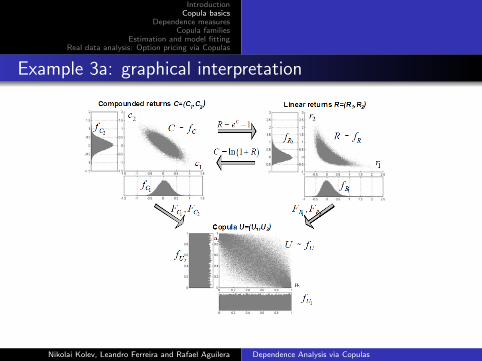
These two types of returns, although calculated on the samestock prices, are different: Rn = eCn − 1 and Cn = ln(1 + Rn);
For example, if stock prices distribution HP is amultivariate log-normal distribution, linear returnsdistribution HR follow a multivariate shifted lognormaldistribution and compounded returns HC follow amultivariate normal distribution.
Nikolai Kolev, Leandro Ferreira and Rafael Aguilera Dependence Analysis via Copulas

IntroductionCopula basics
Dependence measuresCopula families
Estimation and model fittingReal data analysis: Option pricing via Copulas
Example 3a: graphical interpretation
Nikolai Kolev, Leandro Ferreira and Rafael Aguilera Dependence Analysis via Copulas

IntroductionCopula basics
Dependence measuresCopula families
Estimation and model fittingReal data analysis: Option pricing via Copulas
Example 3a: graphical interpretation
Nikolai Kolev, Leandro Ferreira and Rafael Aguilera Dependence Analysis via Copulas

IntroductionCopula basics
Dependence measuresCopula families
Estimation and model fittingReal data analysis: Option pricing via Copulas
Example 3a: graphical interpretation
Nikolai Kolev, Leandro Ferreira and Rafael Aguilera Dependence Analysis via Copulas
IntroductionCopula basics
Dependence measuresCopula families
Estimation and model fittingReal data analysis: Option pricing via Copulas
Example 3a: graphical interpretation
Nikolai Kolev, Leandro Ferreira and Rafael Aguilera Dependence Analysis via Copulas

IntroductionCopula basics
Dependence measuresCopula families
Estimation and model fittingReal data analysis: Option pricing via Copulas
Example 3a: conclusions
Since Rn = eCn − 1 is an increasing transformation α(Cn)and Cn = ln(1 + Rn) is as increasing transformation β(Rn)then CRn,Cn(u, v) = Cβ(Rn),α(Cn)(u, v);
Thus, the copula that joins the linear returns and the copulathat joins the compounded returns is the same.
Nikolai Kolev, Leandro Ferreira and Rafael Aguilera Dependence Analysis via Copulas

IntroductionCopula basics
Dependence measuresCopula families
Estimation and model fittingReal data analysis: Option pricing via Copulas
Example 3a: Commands in R for bivariate Gumbel
Let H1(x , y) be a bivariate Gumbel distribution with copula C(u, v) = uvu+v−uv
,
applying the increasing transformations ex − 1 for marginals obtaining a newdistribution H2(x , y) with the same copula C(u, v).
1 s c a t t e r h i s t = f u n c t i o n ( x , y , x l a b=”” , y l a b=”” , x l=NULL , y l=NULL ,m=NULL){2 p l o t ( x , y , x l a b=x l , y l a b=y l , pch=” . ” , cex =1.5 , main=m)3 h i s t ( x , f r e q=FALSE , x l a b=x l , main=x l )4 h i s t ( y , f r e q=FALSE , x l a b=y l , main=y l )5 }67 #G e t t i n g a sample from H18 H1=sample . gumbel (10000)9 s c a t t e r h i s t (H1 [ , 1 ] , H1 [ , 2 ] , x l a b=”F1” , y l a b=”G1” )
1011 #G e t t i n g a sample from Copula u s i n g m a r g i n a l s from H112 H1 . c o p u l a = 1/(1+ exp(−H1) )13 s c a t t e r h i s t (H1 . c o p u l a [ , 1 ] , H1 . c o p u l a [ , 2 ] , x l a b=”U” , y l a b=”V” )1415 #G e t t i n g a sample from H2 v i a t r a n s f o r m a t i o n16 H2 = exp (H1) − 117 s c a t t e r h i s t (H2 [ , 1 ] , H2 [ , 2 ] , x l=c ( 0 , 5 0 ) , y l=c ( 0 , 5 0 ) , x l a b=”F2” , y l a b=”G2” )1819 #G e t t i n g a sample from Copula u s i n g m a r g i n a l s from H220 H2 . c o p u l a =(H2+1)/ (H2+2)21 s c a t t e r h i s t (H2 . c o p u l a [ , 1 ] , H2 . c o p u l a [ , 2 ] , x l a b=”U” , y l a b=”V” )
Nikolai Kolev, Leandro Ferreira and Rafael Aguilera Dependence Analysis via Copulas

IntroductionCopula basics
Dependence measuresCopula families
Estimation and model fittingReal data analysis: Option pricing via Copulas
Example 3a: Graphs for bivariate Gumbel
Nikolai Kolev, Leandro Ferreira and Rafael Aguilera Dependence Analysis via Copulas

IntroductionCopula basics
Dependence measuresCopula families
Estimation and model fittingReal data analysis: Option pricing via Copulas
Copula of increasing/decreasing transformations
Analogously, we have the following relations:1 If α(x) is strictly increasing in DomX and β(y) is strictly
decreasing in DomY , thenCα(X ),β(Y )(u, v) = u − CXY (u, 1− v);
2 If α(x) is strictly decreasing in DomX and β(y) is strictlyincreasing in DomY , thenCα(X ),β(Y )(u, v) = v − CXY (1− u, v);
3 If α(x) and β(y) are strictly decreasing in DomX andDomY , then Cα(X ),β(Y )(u, v) = u + v − 1 +CXY (1− u, 1− v).
Nikolai Kolev, Leandro Ferreira and Rafael Aguilera Dependence Analysis via Copulas

IntroductionCopula basics
Dependence measuresCopula families
Estimation and model fittingReal data analysis: Option pricing via Copulas
Conditional copula
cu(v) = P(V ≤ v|U = u)
= lim∆u→0
P(V ≤ v|u ≤ U ≤ u + ∆u)
= lim∆u→0
P(V ≤ v,U ≤ u + ∆u)− P(V ≤ v,U ≤ u)
P(u ≤ U ≤ u + ∆u)
= lim∆u→0
C(u + ∆u, v)− C(u, v)
∆u
=∂
∂uC(u, v) = C(v|u)
Definition (Conditional copula)
Conditional copula in u: cu(v) = ∂C(u,v)∂u
= P(V ≤ v |U = u) and conditional copula
in v : cv (u) = ∂C(u,v)∂v
= P(U ≤ u|V = v).
Let us calculate cu(v) of copula C(u, v) = uvu+v−uv
.
cu(v) = ∂∂u
(uv
u+v−uv
)= v(u+v−uv)−uv(1−v)
(u+v−uv)2 = v2
(u+v−uv)2 .
Nikolai Kolev, Leandro Ferreira and Rafael Aguilera Dependence Analysis via Copulas

IntroductionCopula basics
Dependence measuresCopula families
Estimation and model fittingReal data analysis: Option pricing via Copulas
Generating random variables using conditional copulas
P(U ≤ u,V ≤ v) = P(U ≤ u)︸ ︷︷ ︸P(V ≤ v |U = u)︸ ︷︷ ︸u · cu(v) = t
⇒ v = c−1u (t)
Generating random variables using conditional copulas
To generate one observation of a given copula C (u, v):
1 generate two standard uniform observations u and t;
2 fix v = c−1u (t), where c−1
u (t) is inverse of conditional copulacu(t);
3 (u, v) is the required observation.
Nikolai Kolev, Leandro Ferreira and Rafael Aguilera Dependence Analysis via Copulas

IntroductionCopula basics
Dependence measuresCopula families
Estimation and model fittingReal data analysis: Option pricing via Copulas
Example 3b
To generate observation of copula C (u, v) = uvu+v−uv : we
proceed as follows:1 calculate cu(v) = ∂C(u,v)
∂u = ( vu+v−uv )2;
2 generate two independent standard uniform random variables uand t ;
3 from t = cu(v) obtain v = c−1u (t) = u
√t
1−(1−u)√t;
4 set v = u√t
1−(1−u)√t;
5 (u, v) is the required observation of (U,V ).
Nikolai Kolev, Leandro Ferreira and Rafael Aguilera Dependence Analysis via Copulas
IntroductionCopula basics
Dependence measuresCopula families
Estimation and model fittingReal data analysis: Option pricing via Copulas
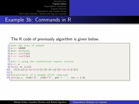
Example 3b: Commands in R
The R code of previously algorithm is given below.
1 #s e t t h e s i z e o f sample2 n <− 100003 #s e t u n i f o r m s4 u <− r u n i f ( n )5 t <− r u n i f ( n )67 #f i x v u s i n g t h e c o n d i t i o n a l c o p u l a i n v e r s e8 v <− u9 f o r ( i i n 1 : n ){
10 v [ i ]=u [ i ]∗ s q r t ( t [ i ] ) /(1−(1−u [ i ] )∗ s q r t ( t [ i ] ) )11 }12 #s c a t t e r p l o t o f a sample (U, V) r e q u i r e d13 p l o t ( u , v , x l a b=”U” , y l a b=”V” , pch = ” . ” , cex = 1 . 5 )
Nikolai Kolev, Leandro Ferreira and Rafael Aguilera Dependence Analysis via Copulas
IntroductionCopula basics
Dependence measuresCopula families
Estimation and model fittingReal data analysis: Option pricing via Copulas
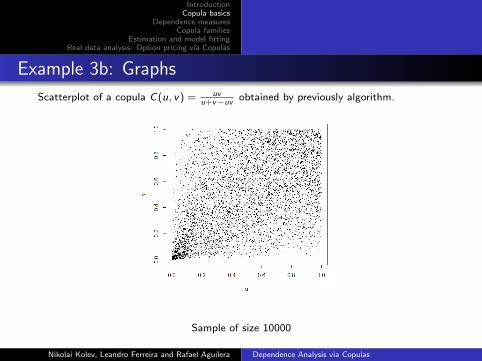
Example 3b: Graphs
Scatterplot of a copula C(u, v) = uvu+v−uv
obtained by previously algorithm.
Sample of size 10000
Nikolai Kolev, Leandro Ferreira and Rafael Aguilera Dependence Analysis via Copulas

IntroductionCopula basics
Dependence measuresCopula families
Estimation and model fittingReal data analysis: Option pricing via Copulas
Application: Monte Carlo integration using copulas
Aim: to obtain the expected value of a continuous functionq(x , y) of a bivariate random vector (X ,Y ) having jointdistribution H(x , y), i.e.
E (q(X ,Y )) =
∫ ∞y=−∞
∫ ∞x=−∞
q(x , y)dH(x , y);
Given the copula C (u, v) = H(F−1(v),G−1(v)) and marginaldistributions F (x) = lim
y→∞H(x , y) and G (y) = lim
x→∞H(x , y),
we can use the following algorithm to approximate the valueof E (q(X ,Y )):
1 generate n observations of the bivariate random vector (X ,Y );2 for each observation i , calculate qi = q(xi , yi ), i = 1, 2, ..., n;3 E (q(X ,Y )) ≈ 1
n
∑ni=1 qi
Nikolai Kolev, Leandro Ferreira and Rafael Aguilera Dependence Analysis via Copulas
IntroductionCopula basics
Dependence measuresCopula families
Estimation and model fittingReal data analysis: Option pricing via Copulas
Example 4
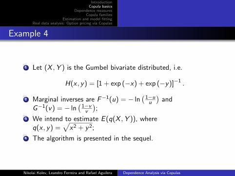
1 Let (X ,Y ) is the Gumbel bivariate distributed, i.e.
H(x , y) = [1 + exp (−x) + exp (−y)]−1 .
2 Marginal inverses are F−1(u) = − ln(
1−uu
)and
G−1(v) = − ln(
1−vv
);
3 We intend to estimate E (q(X ,Y )), whereq(x , y) =
√x2 + y2;
4 The algorithm is presented in the sequel.
Nikolai Kolev, Leandro Ferreira and Rafael Aguilera Dependence Analysis via Copulas

IntroductionCopula basics
Dependence measuresCopula families
Estimation and model fittingReal data analysis: Option pricing via Copulas
Simulation for Example 4
1 For i = 1 to n do:1 generate two standard uniform random variables ui and ti ;
2 fix vi = ui√ti
1−(1−ui )√ti
;
3 fix xi = − ln(
1−uiui
)and yi = − ln
(1−vivi
);
4 calculate qi =√x2i + y2
i
2 obtain E (√X 2 + Y 2) ≈ 1
n
∑ni=1 qi .
Nikolai Kolev, Leandro Ferreira and Rafael Aguilera Dependence Analysis via Copulas
IntroductionCopula basics
Dependence measuresCopula families
Estimation and model fittingReal data analysis: Option pricing via Copulas
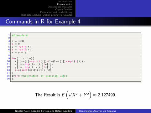
Commands in R for Example 4
1 #Example 423 n = 10004 q = 05 u = r u n i f ( n )6 t = r u n i f ( n )7 x = y = u89 f o r ( i i n 1 : n ){
10 v [ i ]=u [ i ]∗ s q r t ( t [ i ] ) /(1−(1−u [ i ] )∗ s q r t ( t [ i ] ) )11 x [ i ]=− l o g ((1−u [ i ] ) /u [ i ] )12 y [ i ]=− l o g ((1−v [ i ] ) / v [ i ] )13 q=q+s q r t ( x [ i ]ˆ2+ y [ i ] ˆ 2 )14 }15 E=q/n #E s t i m a t i o n o f e x p e c t e d v a l u e16 E
The Result is E(√
X 2 + Y 2)≈ 2.127499.
Nikolai Kolev, Leandro Ferreira and Rafael Aguilera Dependence Analysis via Copulas

IntroductionCopula basics
Dependence measuresCopula families
Estimation and model fittingReal data analysis: Option pricing via Copulas
Dependence measures
We will present four dependence measures between tworandom variables X and Y : the Pearson linear correlationcoefficient and its local version, Kendall’s tau τ(X ,Y ),Spearman’s rho ρ(X ,Y ) and Blest’s measure of rankcorrelation ν(X ,Y );
The measures τ(X ,Y ), ρ(X ,Y ) and ν(X ,Y ) depend only onthe copula C (u, v) corresponding to (X ,Y ). Therefore, theirvalues do not change under strictly increasingtransformations of X and Y (since copula is timeinvariant).
Nikolai Kolev, Leandro Ferreira and Rafael Aguilera Dependence Analysis via Copulas

IntroductionCopula basics
Dependence measuresCopula families
Estimation and model fittingReal data analysis: Option pricing via Copulas
Pearson linear correlation coefficient
Correlation coefficient should be used with caution whenworking outside the class of elliptical distributions. It isdefined by
Corr(X ,Y ) =Cov(X ,Y )√Var(X )Var(Y )
;
Corr(X ,Y ) is defined only when we have finite variancesand it measures linear dependence and assumes values inthe interval [−1, 1];
If two random variables X and Y are independent, thenCorr(X ,Y ) = 0. The inverse statement is not always true.
Nikolai Kolev, Leandro Ferreira and Rafael Aguilera Dependence Analysis via Copulas

IntroductionCopula basics
Dependence measuresCopula families
Estimation and model fittingReal data analysis: Option pricing via Copulas
Pearson linear correlation coefficient - some pitfalls
The Pearson linear correlation coefficient is invariant understrictly increasing linear transformations, i.e.,
Corr(X ,Y ) = Corr(a1X + b1, a2Y + b2);
Corr(X ,Y ) 6= Corr(α(X ), β(Y )), for monotone increasingnon-linear functions α(x) and β(y).
Nikolai Kolev, Leandro Ferreira and Rafael Aguilera Dependence Analysis via Copulas

IntroductionCopula basics
Dependence measuresCopula families
Estimation and model fittingReal data analysis: Option pricing via Copulas
Pearson linear correlation coefficient - some pitfalls
It is not true that given two marginal distributions F (x) andG (y) and a value for the Pearson linear correlation coefficientit is always possible to obtain a bivariate distribution withthese characteristics (the statement is valid for ellipticalworld);
We know that
max(F (x) + G (y)− 1, 0) ≤ H(x , y) ≤ min(F (x),G (y)),
W (x , y) ≤ H(x , y) ≤ M(x , y);
The following relations are valid
rmin = rW ≤ rH = Corr(X ,Y ) ≤ rM = rmax .
Nikolai Kolev, Leandro Ferreira and Rafael Aguilera Dependence Analysis via Copulas

IntroductionCopula basics
Dependence measuresCopula families
Estimation and model fittingReal data analysis: Option pricing via Copulas
Example - McNeil et al. (2005)
Consider two log-normally distributed random variables Xand Y , i.e., lnX ∼ N (0, 1) and lnY ∼ N (0, σ2);
It is important to note that if σ2 6= 1 then X and Y are notof the same type, i.e., do not exist real constants a and bsuch that X =d a + bY , i.e., X and Y are neithercomonotonic nor countermonotonic when σ2 6= 1.
Nikolai Kolev, Leandro Ferreira and Rafael Aguilera Dependence Analysis via Copulas
IntroductionCopula basics
Dependence measuresCopula families
Estimation and model fittingReal data analysis: Option pricing via Copulas
Example - McNeil et al. (2005)
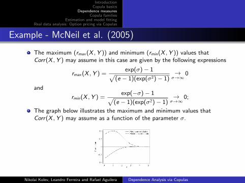
The maximum (rmax(X ,Y )) and minimum (rmin(X ,Y )) values thatCorr(X ,Y ) may assume in this case are given by the following expressions
rmax(X ,Y ) =exp(σ)− 1√
(e − 1)(exp(σ2)− 1)→
σ→∞0
and
rmin(X ,Y ) =exp(−σ)− 1√
(e − 1)(exp(σ2)− 1)→
σ→∞0;
The graph below illustrates the maximum and minimum values thatCorr(X ,Y ) may assume as a function of the parameter σ.
Nikolai Kolev, Leandro Ferreira and Rafael Aguilera Dependence Analysis via Copulas

IntroductionCopula basics
Dependence measuresCopula families
Estimation and model fittingReal data analysis: Option pricing via Copulas
Comments
Note how both limits tend fast to 0 as σ increases.
The graph shows that we may have comonotonic randomvariables (maximally positive dependent) exhibiting values oflinear correlation coefficient close to 0;
Since comonotonicity is the strongest form of positivedependence, this example provides a correction to the usualview that small correlation imply weak dependence;
Therefore, the concept of Pearson linear correlation coefficientis meaningless unless applied in the context of elliptical world.
Nikolai Kolev, Leandro Ferreira and Rafael Aguilera Dependence Analysis via Copulas

IntroductionCopula basics
Dependence measuresCopula families
Estimation and model fittingReal data analysis: Option pricing via Copulas
Local Pearson linear correlation coefficient
While the Pearson linear correlation coefficient
ρ(X ,Y ) =E [(X − E [X ])(Y − E [Y ])]√
E [(X − E [X ])2]E [(Y − E [Y ])2]
is a number in [−1, 1], the local Pearson linear correlationcoefficient
ρlocal(x , y) =E [(X − E (X |Y = y))(Y − E (Y |X = x))]√E (X − E (X |Y = y))2E (Y − E (Y |X = x))2
is a surface depending of (x , y) and ρlocal(x , y) ∈ [−1, 1].
Nikolai Kolev, Leandro Ferreira and Rafael Aguilera Dependence Analysis via Copulas

IntroductionCopula basics
Dependence measuresCopula families
Estimation and model fittingReal data analysis: Option pricing via Copulas
Kendall’s tau
Definition: Kendall’s tau
The population version of Kendall’s tau, τ(X ,Y ), for the bivariate random vector(X ,Y ) is defined as the difference between the probabilities of concordance anddiscordance, i.e.,
τ(X ,Y ) = P[(X − X′)(Y − Y
′) > 0]− P[(X − X
′)(Y − Y
′) < 0],
where (X′,Y′) is an independent copy of (X ,Y ).
Definition: sample version of Kendall’s tau
Let (X1,Y1), . . ., (Xn,Yn) be a sample of (X ,Y ). Denote by Ri and Si the ranks inthe sets X1, . . . ,Xn and Y1, . . . ,Yn, respectively, 1 ≤ i ≤ n. The sample version ofKendall’s tau, τn, is given by
τn =2
n2 − n
∑1≤i<j≤n
sign(Ri − Rj )sign(Si − Sj ).
Nikolai Kolev, Leandro Ferreira and Rafael Aguilera Dependence Analysis via Copulas

IntroductionCopula basics
Dependence measuresCopula families
Estimation and model fittingReal data analysis: Option pricing via Copulas
Kendall’s tau
Theorem
Let (X ,Y ) be a vector of continuous random variables with copulaC (u, v). Then the population Kendall’s tau is given by
τ(X ,Y ) = 4
∫ 1
0
∫ 1
0C (u, v)dC (u, v) − 1,
Note that if U,V ∼ U(0, 1), then
τ(X ,Y ) = 4E [C (U,V )]− 1.
Nikolai Kolev, Leandro Ferreira and Rafael Aguilera Dependence Analysis via Copulas

IntroductionCopula basics
Dependence measuresCopula families
Estimation and model fittingReal data analysis: Option pricing via Copulas
Spearman’s rho
Definition: Spearman’s rho, ρ(X ,Y )
The population Spearman’s rho, ρ(X ,Y ), for the vector (X ,Y ) is
ρ(X ,Y ) = 3P[(X − X′)(Y − Y
′) > 0]− P[(X − X
′)(Y − Y
′′) < 0],
where (X ,Y ), (X′,Y′) and (X
′′,Y′′
) are independent copies of (X ,Y )and X
′and Y
′′are independent.
Definition: sample version Spearman’s rho, ρn
The sample version ρn of Spearman’s rho is
ρn =12
n3 − n
n∑1=1
RiSi −3(n + 1)
n − 1.
Nikolai Kolev, Leandro Ferreira and Rafael Aguilera Dependence Analysis via Copulas

IntroductionCopula basics
Dependence measuresCopula families
Estimation and model fittingReal data analysis: Option pricing via Copulas
Spearman’s rho
Theorem
Let (X ,Y ) be a vector of continuous random variables with copulaC (u, v). Then population Spearman’s rho for (X ,Y ) is given by
ρ(X ,Y ) = 12
∫ 1
0
∫ 1
0
uvdC (u, v) − 3 = 12
∫ 1
0
∫ 1
0
C (u, v)dudv − 3.
Theorem
Let (X ,Y ) be a vector of continuous random variables, X ∼ F (x),Y ∼ G (y), U =d F (X ) ∼ U(0, 1) and V =d G (Y ) ∼ U(0, 1) . Then
ρ(X ,Y ) =Cov(U,V )√Var(U)Var(V )
= Corr(F (X ),G (Y )).
Nikolai Kolev, Leandro Ferreira and Rafael Aguilera Dependence Analysis via Copulas
IntroductionCopula basics
Dependence measuresCopula families
Estimation and model fittingReal data analysis: Option pricing via Copulas
Spearman’s rho
Theorem
Let (X ,Y ) be a vector of continuous random variables with copulaC (u, v). Then the measure Spearman’s rho for (X ,Y ) is given by
ρ(X ,Y ) = 12
∫ 1
0
∫ 1
0[C (u, v)− uv ]dudv .
This result provides a geometric interpretation for thecoefficient ρ(X ,Y ): it is proportional to the volume betweenthe surfaces of copula C (u, v) and independence copulaΠ(u, v) = uv .
Nikolai Kolev, Leandro Ferreira and Rafael Aguilera Dependence Analysis via Copulas

IntroductionCopula basics
Dependence measuresCopula families
Estimation and model fittingReal data analysis: Option pricing via Copulas
The measures of Kendall, Spearman and Pearson
The classical non-parametric Kendall’s tau and Spearman’srho are preferable dependence measures than Corr(X ,Y ),since they are invariant under increasing variabletransformations (since the corresponding copula is invariant);
If X and Y are continuous random variables with copulaC (u, v), then
C (u, v) = M(u, v) = min(u, v)⇔ τ(X ,Y ) = ρ(X ,Y ) = 1;
C (u, v) = W (u, v) = max(u+v−1, 0)⇔ τ(X ,Y ) = ρ(X ,Y ) = −1.
Nikolai Kolev, Leandro Ferreira and Rafael Aguilera Dependence Analysis via Copulas

IntroductionCopula basics
Dependence measuresCopula families
Estimation and model fittingReal data analysis: Option pricing via Copulas
Blest’s measure of rank correlation, ν
The sample versions of Kendalls tau and Spearman’s rho,
τn =2
n2 − n
∑1≤i<j≤n
sign(Ri − Rj)sign(Si − Sj)
and
ρn =12
n3 − n
n∑1=1
RiSi −3(n + 1)
n − 1,
attribute the same importance to the difference betweenthe ranks Ri − Si , i = 1, . . . , n;
Idea: The correlation in the pairs (Ri ,Si ) provides an idea ofconsistency between two ranks and the difference between twoextreme ranks should be emphasized. Thus, Blest (2000)proposed an alternative non-parametric correlation measure ofranks.
Nikolai Kolev, Leandro Ferreira and Rafael Aguilera Dependence Analysis via Copulas

IntroductionCopula basics
Dependence measuresCopula families
Estimation and model fittingReal data analysis: Option pricing via Copulas
Blest’s measure of rank correlation, ν
Definition: sample version of Blest’s measure of rank correlation, νn
The sample version of Blest’s measure of rank correlation, νn, is
νn =2n + 1
n − 1− 12
n2 − n
n∑1=1
Si
(1− Ri
n + 1
)2
.
Definition: Population version of Blest’s measure of rank correlation, ν
The population Blest’s measure of rank correlationfor the vector (X ,Y )is
ν(X ,Y ) = 2− 12∫<2
[1− F 2(x)
]G (y)dH(x , y)
= 2− 12∫
[0,1]2 (1− u)2vdC (u, v),
where ν(X ,Y ) ∈ [0, 1].
Nikolai Kolev, Leandro Ferreira and Rafael Aguilera Dependence Analysis via Copulas

IntroductionCopula basics
Dependence measuresCopula families
Estimation and model fittingReal data analysis: Option pricing via Copulas
Blest’s measure of rank correlation, ν
The extreme values of νn occur when we have (Ri = Si ) or(Ri = n + 1− Si );
Meanwhile is valid the property ν(X ,−Y ) = −ν(X ,Y );
Explicit expressions for ν(X ,Y ) can be obtained for severalbivariate distributions only.
Example. Suppose (X ,Y ) follows a bivariate standard normaldistribution with correlation coefficient r . Thenν(X ,Y ) = ρ(X ,Y ) = 6
π arcsin( r2 ), while τ(X ,Y ) = 2
π arcsin(r).
Nikolai Kolev, Leandro Ferreira and Rafael Aguilera Dependence Analysis via Copulas
IntroductionCopula basics
Dependence measuresCopula families
Estimation and model fittingReal data analysis: Option pricing via Copulas
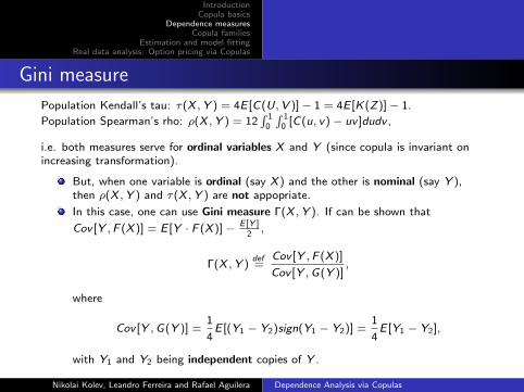
Gini measure
Population Kendall’s tau: τ(X ,Y ) = 4E [C(U,V )]− 1 = 4E [K(Z)]− 1.
Population Spearman’s rho: ρ(X ,Y ) = 12∫ 1
0
∫ 10 [C(u, v)− uv ]dudv ,
i.e. both measures serve for ordinal variables X and Y (since copula is invariant onincreasing transformation).
But, when one variable is ordinal (say X ) and the other is nominal (say Y ),then ρ(X ,Y ) and τ(X ,Y ) are not appopriate.
In this case, one can use Gini measure Γ(X ,Y ). If can be shown that
Cov [Y ,F (X )] = E [Y · F (X )]− E [Y ]2,
Γ(X ,Y )def=
Cov [Y ,F (X )]
Cov [Y ,G(Y )],
where
Cov [Y ,G(Y )] =1
4E [(Y1 − Y2)sign(Y1 − Y2)] =
1
4E [Y1 − Y2],
with Y1 and Y2 being independent copies of Y .
Nikolai Kolev, Leandro Ferreira and Rafael Aguilera Dependence Analysis via Copulas

IntroductionCopula basics
Dependence measuresCopula families
Estimation and model fittingReal data analysis: Option pricing via Copulas
Coefficients of tail dependence
Definition: Upper tail dependence coefficient, λU
Let X and Y be two continuous random variables with copula C(u, v). Theupper tail dependence coefficient λU between X and Y is a property of thecopula C(u, v). It is defined by
λU = limu→1−
C(u, u)
1− u= P(U ≥ u|V ≥ u) =
1− 2u + C(u, v)
1− u,
provided the limit exists and belongs to the interval [0, 1].C(u, v) is the survival copula, given by
C(1− u, 1− v) = 1− u − v + C(u, v).
If λU ∈ (0, 1], then X and Y display upper tail dependence, or extremedependence in the upper tail;
If λU = 0, X and Y are asymptotically independent in the upper tail.
Nikolai Kolev, Leandro Ferreira and Rafael Aguilera Dependence Analysis via Copulas

IntroductionCopula basics
Dependence measuresCopula families
Estimation and model fittingReal data analysis: Option pricing via Copulas
Coefficients of tail dependence
Definition: Lower tail dependence, λL
Let X and Y be two continuous random variables with copulaC (u, v). The lower tail dependence coefficient λL between Xand Y is defined by
λL = P(U ≤ u|V ≤ u) = limu→0+
C (u, u)
u,
provided the limit exists and belong to the interval [0, 1].
If λL ∈ (0, 1], then X and Y display lower tail dependence,or extreme dependence in the lower tail;
If λL = 0, X and Y are asymptotically independent in thelower tail.
Nikolai Kolev, Leandro Ferreira and Rafael Aguilera Dependence Analysis via Copulas

IntroductionCopula basics
Dependence measuresCopula families
Estimation and model fittingReal data analysis: Option pricing via Copulas
Archimedean copulas
Definition (Archimedean copulas)
A copula C (u, v) belongs to the Archimedean family if
C (u, v) = ϕ(ϕ−1(u) + ϕ−1(v)) with (u, v) ∈ [0, 1]2,
for continuous, positive non-increasing and convex functionsϕ : [0,∞)→ [0, 1] such that ϕ(0) = 1. The function ϕ(.) isdenominated generator function of the copula C (u, v).
Typical examples of Archimedean family are the Clayton,Frank and Gumbel copulas presented in the sequel.
Nikolai Kolev, Leandro Ferreira and Rafael Aguilera Dependence Analysis via Copulas
IntroductionCopula basics
Dependence measuresCopula families
Estimation and model fittingReal data analysis: Option pricing via Copulas
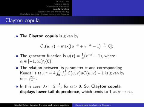
Clayton copula
The Clayton copula is given by
Cα(u, v) = max[(u−α + v−α − 1)−1α , 0];
The generator function is ϕ(t) = 1α(t−α − 1), where
α ∈ [−1,∞)\{0};The relation between its parameter α and correspondingKendall’s tau τ = 4
∫ 10
∫ 10 C (u, v)dC (u, v)− 1 is given by
α = 2τ1−τ ;
In this case, λL = 2−1α , for α > 0. So, Clayton copula
displays lower tail dependence, which tends to 1 as α→∞.
Nikolai Kolev, Leandro Ferreira and Rafael Aguilera Dependence Analysis via Copulas

IntroductionCopula basics
Dependence measuresCopula families
Estimation and model fittingReal data analysis: Option pricing via Copulas
Clayton copula - commands in R
1 l i b r a r y ( c o p u l a )23 # C l a y t o n c o p u l a4 cc <− c l a y t o n C o p u l a ( 2 )5 sample <− r C o p u l a (10000 , cc )6 #S c a t t e r p l o t7 p l o t ( sample , x l a b=”U” , y l a b=”V” , pch = ” . ” , cex = 1 . 5 )89 #D e n s i t y
10 p e r s p ( cc , dCopula , x l a b=”u” , y l a b=” v ” , z l a b=” c ( u , v ) ” )
Nikolai Kolev, Leandro Ferreira and Rafael Aguilera Dependence Analysis via Copulas

IntroductionCopula basics
Dependence measuresCopula families
Estimation and model fittingReal data analysis: Option pricing via Copulas
Clayton copula - scatterplot and copula density
Clayton copula with parameter α = 2
Nikolai Kolev, Leandro Ferreira and Rafael Aguilera Dependence Analysis via Copulas
IntroductionCopula basics
Dependence measuresCopula families
Estimation and model fittingReal data analysis: Option pricing via Copulas
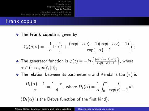
Frank copula
The Frank copula is given by
Cα(u, v) = − 1
αln
{1 +
(exp(−αu)− 1)(exp(−αv)− 1)
exp(−α)− 1
};
The generator function is ϕ(t) = −ln{
(exp(−αt)−1)exp(−α)−1
}, where
α ∈ (−∞,∞)\{0};The relation between its parameter α and Kendall’s tau (τ) is
D1(α)− 1
α=
1− τ4
, where D1(α) =1
α
∫ α
0
t
exp(t)− 1dt
(D1(α) is the Debye function of the first kind).
Nikolai Kolev, Leandro Ferreira and Rafael Aguilera Dependence Analysis via Copulas
IntroductionCopula basics
Dependence measuresCopula families
Estimation and model fittingReal data analysis: Option pricing via Copulas
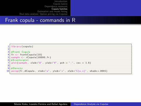
Frank copula - commands in R
1 l i b r a r y ( c o p u l a )23 #Frank Copula4 f r <− f r a n k C o p u l a ( 1 0 )5 sample <− r C o p u l a (10000 , f r )6 #S c a t t e r p l o t7 p l o t ( sample , x l a b=”U” , y l a b=”V” , pch = ” . ” , cex = 1 . 5 )89 #D e n s i t y
10 p e r s p ( f r , dCopula , x l a b=”u” , y l a b=” v ” , z l a b=”C( u , v ) ” , shade =.0001)
Nikolai Kolev, Leandro Ferreira and Rafael Aguilera Dependence Analysis via Copulas

IntroductionCopula basics
Dependence measuresCopula families
Estimation and model fittingReal data analysis: Option pricing via Copulas
Frank copula - scatterplot and copula density
Frank copula with parameter α = 10
Nikolai Kolev, Leandro Ferreira and Rafael Aguilera Dependence Analysis via Copulas

IntroductionCopula basics
Dependence measuresCopula families
Estimation and model fittingReal data analysis: Option pricing via Copulas
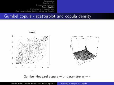
Gumbel-Hougard copula
The Gumbel-Hougard copula is given by
Cα(u, v) = exp
{−[(− ln u)α + (− ln v)α]
α−1}
;
The generator function is given by ϕ(t) = (− ln t)α, whereα ∈ [1,∞);
The relation between its parameter α and Kendall’s τ isα = 1
1−τ ;
λU = 2− 21α . If α > 1, the copula displays upper tail
dependence. This dependence tends to 1 as α→∞, (whatis to be expected, since in this situation, the Gumbel-Hougardcopula tends to the comonotonic copula).
Nikolai Kolev, Leandro Ferreira and Rafael Aguilera Dependence Analysis via Copulas

IntroductionCopula basics
Dependence measuresCopula families
Estimation and model fittingReal data analysis: Option pricing via Copulas
Gumbel copula - commands in R
1 l i b r a r y ( c o p u l a )23 # Gumbel c o p u l a4 gu <− gumbelCopula ( 4 )5 sample <− r C o p u l a (10000 , gu )6 #S c a t t e r p l o t7 p l o t ( sample , x l a b=”U” , y l a b=”V” , pch = ” . ” , cex = 1 . 5 )89 #D e n s i t y
10 p e r s p ( gu , dCopula , x l a b=”u” , y l a b=” v ” , z l a b=”C( u , v ) ” )
Nikolai Kolev, Leandro Ferreira and Rafael Aguilera Dependence Analysis via Copulas
IntroductionCopula basics
Dependence measuresCopula families
Estimation and model fittingReal data analysis: Option pricing via Copulas
Gumbel copula - scatterplot and copula density
Gumbel-Hougard copula with parameter α = 4
Nikolai Kolev, Leandro Ferreira and Rafael Aguilera Dependence Analysis via Copulas

IntroductionCopula basics
Dependence measuresCopula families
Estimation and model fittingReal data analysis: Option pricing via Copulas
Standard univariate normal distribution
The distribution function of a random variable X that followsa standard normal N(0, 1) distribution is given by
Φ(x) = P(X ≤ x) =1√2π
∫ x
−∞exp(−t2/2)dt
Nikolai Kolev, Leandro Ferreira and Rafael Aguilera Dependence Analysis via Copulas

IntroductionCopula basics
Dependence measuresCopula families
Estimation and model fittingReal data analysis: Option pricing via Copulas
Bivariate normal distribution
The density function of a random vector (X ,Y ) that follows astandard bivariate normal distribution with correlationcoefficient ρ is given by
φ2,ρ(x , y) =1
2π√
1− ρ2exp
(− 1
2(1− ρ2)
[x2 + y2 − 2ρxy
]),
where −∞ < x <∞, −1 ≤ ρ ≤ 1 and X ,Y ∼ N(0, 1);
The corresponding joint distribution function is given by
Φ2,ρ(x , y) = P(X ≤ x ,Y ≤ y) =
∫ x
−∞
∫ y
−∞φ2,ρ(u, v)dudv .
Nikolai Kolev, Leandro Ferreira and Rafael Aguilera Dependence Analysis via Copulas

IntroductionCopula basics
Dependence measuresCopula families
Estimation and model fittingReal data analysis: Option pricing via Copulas
Univariate t−Student distribution
A random variable η follows the Student−t distribution with
ν degrees of freedom whenever it can be written as ηd= X√
ξν
,
X ∼ N (0, 1) and is independent of ξ ∼ χ2ν ;
The density function is given by
tν(x) =Γ(ν+1
2
)√νπΓ
(ν2
)(1 +x2
ν
)− ν+12
,
where x ∈ < and ν > 0.
Nikolai Kolev, Leandro Ferreira and Rafael Aguilera Dependence Analysis via Copulas

IntroductionCopula basics
Dependence measuresCopula families
Estimation and model fittingReal data analysis: Option pricing via Copulas
Bivariate t-Student distribution
A random vector T = (T1,T2) follows a bivariate t-Studentdistribution with ν degrees of freedom whenever it can be writtenas
(T1,T2) =
X√ξν
,Y√ξν
.
The bivariate random vector (X ,Y ) has standard bivariate normaldistribution with correlation coefficient ρ being independent ofξ ∼ χ2
ν ;
The joint density function is given by
tν,ρ(x , y) =1
2π√
1− ρ2
{1 +
x2 − 2ρxy + y2
ν(1− ρ2)2
}− ν+22
,
where x , y ∈ (−∞,∞), ρ ∈ [−1, 1].
Nikolai Kolev, Leandro Ferreira and Rafael Aguilera Dependence Analysis via Copulas

IntroductionCopula basics
Dependence measuresCopula families
Estimation and model fittingReal data analysis: Option pricing via Copulas
Elliptical distributions
The name ”elliptical” comes from the elliptical (sum ofsquares) form of the level curves of the joint densityfunction, i.e., f (x , y) = a = constant;
The bivariate random vector Z = (Z1,Z2) follows a sphericaldistribution if and only if its characteristic function can berepresented by E [exp(itTZ )] = ψ(z2
1 + z22 ), t ∈ <2, for some
function ψ : < → <;
The bivariate random vector W = (W1,W2) follows aelliptical distribution if W = µ+ AZ, where µ ∈ <2,A ∈ <2 ×<2 and Z follows a spherical distribution;
Particular cases of elliptical distributions are the bivariatenormal as well as the bivariate t-Student distributions.
Nikolai Kolev, Leandro Ferreira and Rafael Aguilera Dependence Analysis via Copulas

IntroductionCopula basics
Dependence measuresCopula families
Estimation and model fittingReal data analysis: Option pricing via Copulas
Elliptical copulas
Elliptical copulas became very popular in finance and riskmanagement because they are easily implemented. The ease inobtaining the marginal distribution functions is another advantagewhen one uses this elliptical copulas for forecast, see Frees e Wang(2005);
”Elliptical” because they are associated with a quadratic form ofcorrelation coefficient between the marginals. It means, theelliptical family of copulas is symmetric. The dependence structureis determined by the correlation matrix;
The Gaussian copula and the t-copula are particular cases ofelliptical copulas, with dispersion matrix inherited from theelliptical distributions (correlation coefficient ρ). The t-copulapossesses an additional degrees of freedom parameter ν, whichmodify the shape of the copula for given level of dependencegoverned by ρ.
Nikolai Kolev, Leandro Ferreira and Rafael Aguilera Dependence Analysis via Copulas
IntroductionCopula basics
Dependence measuresCopula families
Estimation and model fittingReal data analysis: Option pricing via Copulas
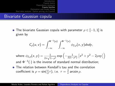
Bivariate Gaussian copula
The bivariate Gaussian copula with parameter ρ ∈ [−1, 1] isgiven by
Cρ(u, v) =
∫ Φ−1(u)
−∞
∫ Φ−1(v)
−∞φ2,ρ(x , y)dxdy ,
where φ2,ρ(x , y) = 1
2π√
1−ρ2exp
(− 1
2(1−ρ2)
[x2 + y2 − 2ρxy
])and Φ−1(·) is the inverse of standard normal distribution;
The relation between Kendall’s tau and the correlationcoefficient is ρ = sin(π2 τ), i.e. τ = 2
π arcsin ρ.
Nikolai Kolev, Leandro Ferreira and Rafael Aguilera Dependence Analysis via Copulas

IntroductionCopula basics
Dependence measuresCopula families
Estimation and model fittingReal data analysis: Option pricing via Copulas
Tail dependence of Gaussian copula
Due to symmetry of Gaussian copula we have equal upper andlower tail dependence coefficients, i.e. λU = λL = λ with
λ = 2 limx→−∞
Φ
(x√
1− ρ√1 + ρ
)= 0.
Interpretation: Independently of the value of the correlationcoefficient, asymptotically the Gaussian copula displaysindependence in both tails, meaning that regardless of howhigh a correlation coefficient we choose, if we go far enough intothe tail, extreme events appear to occur independently ineach margin.
Nikolai Kolev, Leandro Ferreira and Rafael Aguilera Dependence Analysis via Copulas

IntroductionCopula basics
Dependence measuresCopula families
Estimation and model fittingReal data analysis: Option pricing via Copulas
Density of a bivariate copula
To calculate the density c(u, v) of a bivariate copula proceed as follows
c(u, v) =∂2
∂u ∂vC (u, v) =
∂2
∂u ∂vH(F−1(u),G−1(v)) =
h(F−1(u),G−1(v))
f (F−1(u))g(G−1(v)).
Therefore,
If we know the bivariate density h(x , y), then we can obtain f (x),F−1(x), g(y) and G−1(y), to calculate
c(u, v) =h(F−1(u),G−1(v))
f (F−1(u))g(G−1(v));
If we know copula density c(u, v) and the marginal densitiesf (x) and g(y), we can calculate F (x) and G (y). Thus,
h(x , y) = c(F (x),G (y))f (x)g(y).
Nikolai Kolev, Leandro Ferreira and Rafael Aguilera Dependence Analysis via Copulas

IntroductionCopula basics
Dependence measuresCopula families
Estimation and model fittingReal data analysis: Option pricing via Copulas
Density of the bivariate Gumbel logistic copula
The copula corresponding to the bivariate Gumbel logisticdistribution is given by
C (u, v) = H(F−1(u),G−1(v)) =uv
u + v − uv;
Its density function is
c(u, v) =∂2
∂u ∂v
(uv
u + v − uv
)=
2uv
(u + v − uv)3.
Nikolai Kolev, Leandro Ferreira and Rafael Aguilera Dependence Analysis via Copulas
IntroductionCopula basics
Dependence measuresCopula families
Estimation and model fittingReal data analysis: Option pricing via Copulas
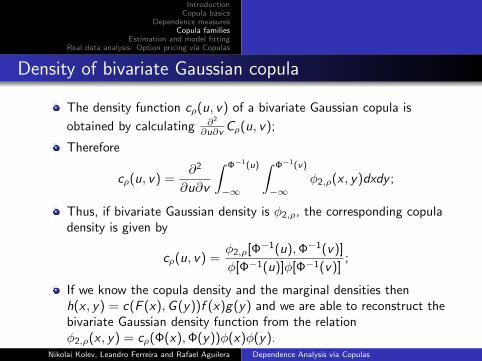
Density of bivariate Gaussian copula
The density function cρ(u, v) of a bivariate Gaussian copula is
obtained by calculating ∂2
∂u∂v Cρ(u, v);
Therefore
cρ(u, v) =∂2
∂u∂v
∫ Φ−1(u)
−∞
∫ Φ−1(v)
−∞φ2,ρ(x , y)dxdy ;
Thus, if bivariate Gaussian density is φ2,ρ, the corresponding copuladensity is given by
cρ(u, v) =φ2,ρ[Φ−1(u),Φ−1(v)]
φ[Φ−1(u)]φ[Φ−1(v)];
If we know the copula density and the marginal densities thenh(x , y) = c(F (x),G (y))f (x)g(y) and we are able to reconstruct thebivariate Gaussian density function from the relationφ2,ρ(x , y) = cρ(Φ(x),Φ(y))φ(x)φ(y).
Nikolai Kolev, Leandro Ferreira and Rafael Aguilera Dependence Analysis via Copulas

IntroductionCopula basics
Dependence measuresCopula families
Estimation and model fittingReal data analysis: Option pricing via Copulas
R code to visualize the density functions of a standardbivariate normal distribution and its copula
1 l i b r a r y ( mvtnorm )2 d=2; x = seq (−3 ,3 ,6∗ . 0 2 5 ) ; x . cop = seq ( 0 , 1 , . 0 2 5 )3 #C o v a r i a n c e m a t r i x4 c1<−c ( 1 , . 7 ) ; c2<−c ( . 7 , 1 ) ; R=c b i n d ( c1 , c2 )5 dens = dens . cop = dens2 = dens3 = m a t r i x ( 0 , nrow=l e n g t h ( x ) , n c o l=l e n g t h ( x ) )67 #C a l c u l a t i n g d e n s i t i e s o f d i s t r i b u t i o n s8 f o r ( i i n 1 : dim ( dens ) [ 1 ] )9 { f o r ( j i n 1 : dim ( dens ) [ 2 ] )
10 {dens [ i , j ] = dmvnorm ( x=c ( x [ i ] , x [ j ] ) , mean=r e p ( 0 , d ) , s igma=R)11 dens . cop [ i , j ] = dmvnorm ( x=c ( qnorm ( x . cop [ i ] ) , qnorm ( x . cop [ j ] ) ) , mean=r e p ( 0 , d ) ,
s igma=R) / ( dnorm ( qnorm ( x . cop [ i ] ) )∗dnorm ( qnorm ( x . cop [ j ] ) ) )}}1213 #D e n s i t y o f a s t a n d a r d b i v a r i a t e normal d i s t r i b u t i o n14 p e r s p ( x , x , dens , x l a b=” x ” , y l a b=” y ” , z l a b=” f ( x , y ) ” , shade = 0 . 7 5 )15 #D e n s i t y o f normal c o p u l a16 p e r s p ( x . cop , x . cop , dens . cop , x l a b=”u” , y l a b=” v ” , z l a b=” c ( u , v ) ” , shade = 0 . 7 5 )
Nikolai Kolev, Leandro Ferreira and Rafael Aguilera Dependence Analysis via Copulas

IntroductionCopula basics
Dependence measuresCopula families
Estimation and model fittingReal data analysis: Option pricing via Copulas
Graph of the standard bivariate normal density function
The density φ2,ρ(x , y) of a standard bivariate normal distribution,with ρ = 0.7
Nikolai Kolev, Leandro Ferreira and Rafael Aguilera Dependence Analysis via Copulas

IntroductionCopula basics
Dependence measuresCopula families
Estimation and model fittingReal data analysis: Option pricing via Copulas
Graphs of two standard univariate normal densities
divided by the product of the corresponding marginal standardnormal densities φ(x) and φ(y) ...
Nikolai Kolev, Leandro Ferreira and Rafael Aguilera Dependence Analysis via Copulas

IntroductionCopula basics
Dependence measuresCopula families
Estimation and model fittingReal data analysis: Option pricing via Copulas
Graph of the Gaussian copula density
provides the Gaussian copula density
cρ(u, v) =φ2,ρ(Φ−1(u),Φ−1(v))
φ(Φ−1(u))φ(Φ−1(v))
Nikolai Kolev, Leandro Ferreira and Rafael Aguilera Dependence Analysis via Copulas

IntroductionCopula basics
Dependence measuresCopula families
Estimation and model fittingReal data analysis: Option pricing via Copulas
Summarizing
The standard bivariate normal density φ2,ρ divided by the productof the corresponding marginal standard normal density functions
results in the bivariate Gaussian copula density cρ(u, v)
Nikolai Kolev, Leandro Ferreira and Rafael Aguilera Dependence Analysis via Copulas

IntroductionCopula basics
Dependence measuresCopula families
Estimation and model fittingReal data analysis: Option pricing via Copulas
Generating a density of new bivariate distribution
If we multiply the bivariate Gaussian copula density cρ(u, v) by twoarbitrarily density functions we will obtain a new bivariate density
function: h(x , y) = cρ(F (x),G (y))f (x)g(y). It keeps thedependence structure of the standard bivariate normal distribution
but the marginal distributions are just F (x) and G (y)
Nikolai Kolev, Leandro Ferreira and Rafael Aguilera Dependence Analysis via Copulas

IntroductionCopula basics
Dependence measuresCopula families
Estimation and model fittingReal data analysis: Option pricing via Copulas
Generating a density of new bivariate distribution
Commands in R to generating a density of a new bivariatedistribution with gamma(5,1) and N(0, 1) marginals
1 #C a l c u l a t i n g d e n s i t i e s o f d i s t r i b u t i o n s2 f o r ( i i n 1 : dim ( dens ) [ 1 ] )3 { f o r ( j i n 1 : dim ( dens ) [ 2 ] )4 {#u s i n g normal and normal as m a r g i n a l s5 dens2 [ i , j ]= dens . cop [ i , j ]∗( dnorm ( x [ i ] )∗dnorm ( x [ j ] ) )6 #u s i n g gamma and normal as m a r g i n a l s7 dens3 [ i , j ]= dens . cop [ i , j ]∗(dgamma( x [ i ] , shape =5, s c a l e =1)∗dnorm ( x [ j ] ) )}}89 #D e n s i t y o f t h e d e n s i t y u s i n g normal m a r g i n a l s
10 p e r s p ( x , x , dens2 , x l a b=” x ” , y l a b=” y ” , z l a b=” f ( x , y ) ” )11 #D e n s i t y o f t h e d e n s i t y u s i n g gamma and normal m a r g i n a l s12 p e r s p ( x , x , dens3 , x l a b=” x ” , y l a b=” y ” , z l a b=” f ( x , y ) ” , x l i m=c (−3 ,3) , y l i m=c (−3 ,3) , t h e t a
=80, shade = 0 . 7 5 , expand =0.8)
Nikolai Kolev, Leandro Ferreira and Rafael Aguilera Dependence Analysis via Copulas

IntroductionCopula basics
Dependence measuresCopula families
Estimation and model fittingReal data analysis: Option pricing via Copulas
Bivariate t-copula
The bivariate t-copula is given by
Cν,ρ(u, v) = Tν,ρ(T−1ν (u),T−1
ν (v)),
where ρ ∈ [−1, 1], Tν(.) is the univariate distribution functionof a random variable that follow the t-Student distributionwith ν degrees of freedom and Tν,ρ(., .) is the jointdistribution function of a random bivariate vectorT = (T1,T2) that follows a bivariate t-Student distributionwith ν degrees of freedom;
The corresponding bivariate t-copula density is
cν,ρ(u, v) =tν,ρ(T−1
ν (u),T−1ν (v))
tν(T−1ν (u))tν(T−1
ν (v)).
Nikolai Kolev, Leandro Ferreira and Rafael Aguilera Dependence Analysis via Copulas

IntroductionCopula basics
Dependence measuresCopula families
Estimation and model fittingReal data analysis: Option pricing via Copulas
Tail dependence of t-copula
Due to the symmetry of t-copula for tail dependence coefficientwe have
λU = λL = λ = 2Tν+1
(−
√(ν + 1)(1− ρ)
1 + ρ
),
when Tν+1 means the distribution function of a random variablethat follows t-Student distribution with ν + 1 degrees of freedom.
Provided ρ > −1, t-copula is asymptotically dependent in bothtails.
Nikolai Kolev, Leandro Ferreira and Rafael Aguilera Dependence Analysis via Copulas
IntroductionCopula basics
Dependence measuresCopula families
Estimation and model fittingReal data analysis: Option pricing via Copulas
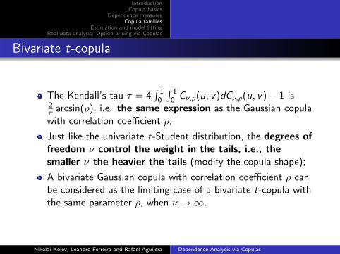
Bivariate t-copula
The Kendall’s tau τ = 4∫ 1
0
∫ 10 Cν,ρ(u, v)dCν,ρ(u, v)− 1 is
2π arcsin(ρ), i.e. the same expression as the Gaussian copulawith correlation coefficient ρ;
Just like the univariate t-Student distribution, the degrees offreedom ν control the weight in the tails, i.e., thesmaller ν the heavier the tails (modify the copula shape);
A bivariate Gaussian copula with correlation coefficient ρ canbe considered as the limiting case of a bivariate t-copula withthe same parameter ρ, when ν →∞.
Nikolai Kolev, Leandro Ferreira and Rafael Aguilera Dependence Analysis via Copulas
IntroductionCopula basics
Dependence measuresCopula families
Estimation and model fittingReal data analysis: Option pricing via Copulas
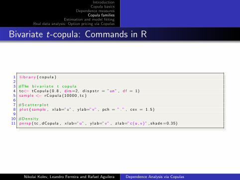
Bivariate t-copula: Commands in R
1 l i b r a r y ( c o p u l a )23 #The b i v a r i a t e t c o p u l a4 t c<− tCopu la ( 0 . 8 , dim=2, d i s p s t r = ”un” , d f = 1)5 sample <− r C o p u l a (10000 , t c )67 #S c a t t e r p l o t8 p l o t ( sample , x l a b=”u” , y l a b=” v ” , pch = ” . ” , cex = 1 . 5 )9
10 #D e n s i t y11 p e r s p ( tc , dCopula , x l a b=”u” , y l a b=” v ” , z l a b=” c ( u , v ) ” , shade =0.35)
Nikolai Kolev, Leandro Ferreira and Rafael Aguilera Dependence Analysis via Copulas

IntroductionCopula basics
Dependence measuresCopula families
Estimation and model fittingReal data analysis: Option pricing via Copulas
Bivariate t-copula - scatterplot and density
Bivariate t-copula with parameters ρ = 0.8 and ν = 1
Nikolai Kolev, Leandro Ferreira and Rafael Aguilera Dependence Analysis via Copulas

IntroductionCopula basics
Dependence measuresCopula families
Estimation and model fittingReal data analysis: Option pricing via Copulas
Other examples of copulas
Besides the families of copulas we have already seen there areothers that exhibit tail dependence (frequently used inpractice). We will consider
Rotated Gumbel Copula (lower tail);
Symmetrized Joe-Clayton Copula (upper and lower tail).
Nikolai Kolev, Leandro Ferreira and Rafael Aguilera Dependence Analysis via Copulas

IntroductionCopula basics
Dependence measuresCopula families
Estimation and model fittingReal data analysis: Option pricing via Copulas
Rotated Gumbel copula
The Rotated Gumbel copula is given by
CRG (u, v |α) = u + v − 1 + Cα(1− u, 1− v |α),
where α ∈ [1,+∞) and Cα is the Gumbel-Hougard copula,which is given by
Cα(u, v) = exp
{−[(− ln u)α + (− ln v)α]
α−1}
;
This copula exhibits only lower tail dependence.
Nikolai Kolev, Leandro Ferreira and Rafael Aguilera Dependence Analysis via Copulas

IntroductionCopula basics
Dependence measuresCopula families
Estimation and model fittingReal data analysis: Option pricing via Copulas
Rotated Gumbel copula: Commands in R
1 l i b r a r y ( ”CDVine” )2 # s i m u l a t e from a b i v a r i a t e Rotated−Gumbel (90 d e g r e e s ) c o p u l a3 rg90 = BiCopSim (10000 ,24 ,−3)4 p l o t ( rg90 , x l a b=”U” , y l a b=”V” , pch = ” . ” , cex =1.5)56 # s i m u l a t e from a b i v a r i a t e Rotated−Gumbel (270 d e g r e e s ) c o p u l a7 rg270 = BiCopSim (10000 ,34 ,−3)8 p l o t ( rg270 , x l a b=”U” , y l a b=”V” , pch = ” . ” , cex =1.5)
Nikolai Kolev, Leandro Ferreira and Rafael Aguilera Dependence Analysis via Copulas

IntroductionCopula basics
Dependence measuresCopula families
Estimation and model fittingReal data analysis: Option pricing via Copulas
Rotated Gumbel copula - scatterplot
Rotated Gumbel copula with α = 90 and α = 270
Scatterplot of a sample of size 10000
Nikolai Kolev, Leandro Ferreira and Rafael Aguilera Dependence Analysis via Copulas

IntroductionCopula basics
Dependence measuresCopula families
Estimation and model fittingReal data analysis: Option pricing via Copulas
Symmetrized Joe-Clayton copula
The Symmetrized Joe-Clayton copula CSJC is given by
CSJC (u, v |τU , τL) =1
2· [CJC (u, v |τU , τL)
+CJC (1− u, 1− v |τU , τL) + u + v − 1],
where CJC is the Joe-Clayton copula represented by
CJC (u, v |τU , τL) = 1− (1− {[1− (1− u)κ]−γ
+[1− (1− v)κ]−γ − 1}−1/γ)−1/κ,
with κ = 1/ log2(2− τU), γ = −1/ log2(τL) and τU , τL ∈ (0, 1).
The SJC has both upper and lower tail dependence parameters. Itsown dependence parameters, τU and τL, are the measures of dependenceof the upper and lower tail, respectively. Furthermore, τU and τL rangefreely and are not dependent on each other.
Nikolai Kolev, Leandro Ferreira and Rafael Aguilera Dependence Analysis via Copulas

IntroductionCopula basics
Dependence measuresCopula families
Estimation and model fittingReal data analysis: Option pricing via Copulas
Power copula
Let C be an arbitrary copula and define the power copula PC
as following
PC (u, v) = uθ1vθ2C (u1−θ1 , v1−θ2),
where the parameters θ1, θ2 ∈ [0, 1].
When we choose θ1 = θ2 = 0 then PC (u, v) = C (u, v).
In financial derivatives, for example, the parameters θ1 and θ2
control the slope and the curvature of the impliedvolatility smile.
Nikolai Kolev, Leandro Ferreira and Rafael Aguilera Dependence Analysis via Copulas

IntroductionCopula basics
Dependence measuresCopula families
Estimation and model fittingReal data analysis: Option pricing via Copulas
Comparison of a Gaussian copula and Power Gaussian copula densities
Gaussian copula,
ρ = 0.7.
Power Gaussian copula,
ρ = 0.7, θ1 = 0.7 and θ2 = 0.3.
Nikolai Kolev, Leandro Ferreira and Rafael Aguilera Dependence Analysis via Copulas

IntroductionCopula basics
Dependence measuresCopula families
Estimation and model fittingReal data analysis: Option pricing via Copulas
Scatterplot of Power Gaussian copula
Sampling of Power Gaussian copula,
ρ = 0.7, θ1 = 0.7 and θ2 = 0.3.
Nikolai Kolev, Leandro Ferreira and Rafael Aguilera Dependence Analysis via Copulas
IntroductionCopula basics
Dependence measuresCopula families
Estimation and model fittingReal data analysis: Option pricing via Copulas
Example: Marshall-Olkin copula
If our base copula is
M(u, v) = min(u, v),
then the resulting power copula is
PM(u, v) = uθ1vθ2 min(u1−θ1 , v1−θ2
),
being the Marshall-Olkin copula.
Nikolai Kolev, Leandro Ferreira and Rafael Aguilera Dependence Analysis via Copulas
IntroductionCopula basics
Dependence measuresCopula families
Estimation and model fittingReal data analysis: Option pricing via Copulas
Kendall distribution
Recall that, according to Probability Integral Transform
U = F (X ) ∼ U(0, 1), i.e. P(U ≤ w) = w
”Bivariate Prob. Int. Transform” is the Kendall distribution
K (w) = P[H(X ,Y ) ≤ w) = P[C (X ,Y ) ≤ w), w ∈ [0, 1];
K (w) is univariate summary of dependence embodied in C ;
K (w) depends only on the copula C associated with H, and hencenot on the marginals F and G ;
w ≤ K (w) ≤ 1, w ∈ [0, 1];
If U and V are independent the
K (w) = P(UV ≤ w) = w − w log(w);
In general, K (w) 6= w , i.e. H(X ,Y ) is not U(0, 1).Nikolai Kolev, Leandro Ferreira and Rafael Aguilera Dependence Analysis via Copulas

IntroductionCopula basics
Dependence measuresCopula families
Estimation and model fittingReal data analysis: Option pricing via Copulas
Empirical copula and empirical Kendall distribution
Let (X1,Y1), . . . , (Xn,Yn), n ≥ 2, be a random sample of a continuousdistribution and let X(i) and Y(j) be the order statistics of the sample.
The empirical copula Cn is defined as
Cn =1
n
(number of points (Xm,Ym) such that Xm ≤ X(i) and Ym ≤ Y(j)
).
An equivalent form of empirical copula is given by
Cn(u, v) =1
n
n∑i=1
1(ui ≤ u, vi ≤ v),
where 1(·) is the indicator function,
ui =rank(Xi )
n + 1=
Ri
n + 1and vi =
rank(Yi )
n + 1=
Si
n + 1;
The empirical Kendall distribution function Kn(t) for all t is given by
Kn(t) =1
n(number of points (Xm,Ym) such that Cn(u, v) ≤ t) .
Nikolai Kolev, Leandro Ferreira and Rafael Aguilera Dependence Analysis via Copulas
IntroductionCopula basics
Dependence measuresCopula families
Estimation and model fittingReal data analysis: Option pricing via Copulas
Construction of Kendall plot
The Kendall plot (K-plot) is based on Kendall distributionfunction K (w) = P(C (U,V ) ≤ w) = P(H(X ,Y ) ≤ w) and itis analog of the classic Q-Q plot. It is introduced by Genestand Boies (2003) to evaluate the dependence structure in abivariate sample. The construction follows the steps:
1 Calculate Hi =#{j 6=i :Xj≤Xi ,Yj≤Yi}
n−1 for each i = 1, . . . , n;2 Order the H ′i s, such that H(1) ≤ . . . ≤ H(n);3 Plot the pairs (Wi :n,H(i)), 1 ≤ i ≤ n, where Wi :n represents
the expected value of the ith order statistic in a sample withsize n of the distribution K0(w) = w − w log(w), 0 ≤ w ≤ 1(Kendall distribution in independence case).
Nikolai Kolev, Leandro Ferreira and Rafael Aguilera Dependence Analysis via Copulas
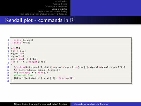
IntroductionCopula basics
Dependence measuresCopula families
Estimation and model fittingReal data analysis: Option pricing via Copulas
Kendall plot - commands in R
1 l i b r a r y ( CDVine )2 l i b r a r y (MASS)34 n<−2505 nu<−c ( 0 , 0 )6 s igma1<−17 sigma2<−18 rho<−seq (−1 ,1 ,0 .2)9 f o r ( i i n 1 : l e n g t h ( rho ) )
10 {11 S<−c b i n d ( c ( s igma1 ˆ2 , rho [ i ]∗s igma1∗s igma2 ) , c ( rho [ i ]∗s igma1∗sigma2 , s igma2 ˆ2) )12 X<−mvrnorm ( n=n , mu=nu , Sigma=S )13 v i p t<−a p p l y (X, 2 , rank ) /n14 #K e n d a l l P l o t15 BiCopKPlot ( v i p t [ , 1 ] , v i p t [ , 2 ] , f a m i l y= ’B ’ )16 }
Nikolai Kolev, Leandro Ferreira and Rafael Aguilera Dependence Analysis via Copulas

IntroductionCopula basics
Dependence measuresCopula families
Estimation and model fittingReal data analysis: Option pricing via Copulas
Animation of Kendall plot
Nikolai Kolev, Leandro Ferreira and Rafael Aguilera Dependence Analysis via Copulas

IntroductionCopula basics
Dependence measuresCopula families
Estimation and model fittingReal data analysis: Option pricing via Copulas
Tail copula
Remind that
λL = limu→0+
C (u, u)
uand λU = lim
u→0+
C (u, u)
u
can be regarded as directional derivatives of C (u, v). Assumingdifferent directions (uq, vq), we get lower tail copulas. The lowertail copula ΛL(u, v) and upper tail copula ΛU(u, v) associated withX and Y is a function of their copula C (u, v) or survival copulaC (u, v), respectively and are defined by
ΛL(u, v) = limq→0+
C (uq, vq)
qand ΛU(u, v) = lim
q→0+
C (uq, vq)
q.
for all (u, v) ∈ [0,∞)2 = R2+.
Nikolai Kolev, Leandro Ferreira and Rafael Aguilera Dependence Analysis via Copulas
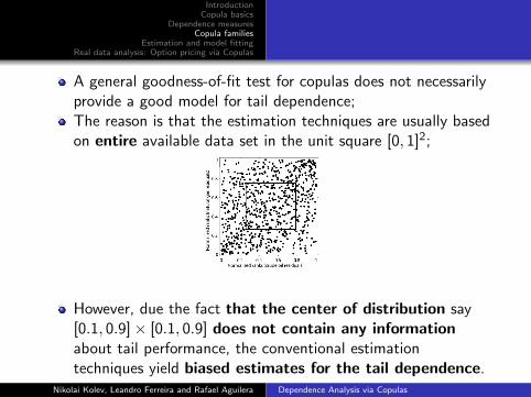
IntroductionCopula basics
Dependence measuresCopula families
Estimation and model fittingReal data analysis: Option pricing via Copulas
A general goodness-of-fit test for copulas does not necessarilyprovide a good model for tail dependence;The reason is that the estimation techniques are usually basedon entire available data set in the unit square [0, 1]2;
However, due the fact that the center of distribution say[0.1, 0.9]× [0.1, 0.9] does not contain any informationabout tail performance, the conventional estimationtechniques yield biased estimates for the tail dependence.
Nikolai Kolev, Leandro Ferreira and Rafael Aguilera Dependence Analysis via Copulas

IntroductionCopula basics
Dependence measuresCopula families
Estimation and model fittingReal data analysis: Option pricing via Copulas
In order to overcome this problem, we apply the concept of tailcopulas being function of the underlying copula (which describesthe dependence structure in the tail of multivariate distributions)
ΛL(u, v) = limq→0+
C (uq, vq)
qand ΛU(u, v) = lim
q→0+
C (uq, vq)
q;
The tail copulas can be considered as a local version of taildependence coefficients λL and λU because
ΛL(1, 1) = λL and ΛU(1, 1) = λU ;
To obtain estimators that are more robust with respect to thecenter of distribution, there are 2 approaches:
- to use tail copula (which enable to model tail dependence ofarbitrary form);
- to rely a extreme value copula (Pareto one, say).
Nikolai Kolev, Leandro Ferreira and Rafael Aguilera Dependence Analysis via Copulas
IntroductionCopula basics
Dependence measuresCopula families
Estimation and model fittingReal data analysis: Option pricing via Copulas
Tail empirical copula
If Cn is the empirical copula, the empirical lower tail copula is defined by
ΛL,n(u, v) =n
kCn
(ku
n,kv
n
)≈ 1
k
n∑i=1
1
(ui ≤
ku
n + 1, vi ≤
kv
n + 1
);
If Cn is the empirical survival copula, the empirical upper tail copula is
ΛU,n(u, v) =n
kC n
(ku
n,kv
n
)≈ 1
k
n∑i=1
1
(ui >
n − ku
n + 1, vi >
n − kv
n + 1
)for some parameter k ∈ {1, · · · , n} (see Schmidt and Stadtmller (2006)).
Nikolai Kolev, Leandro Ferreira and Rafael Aguilera Dependence Analysis via Copulas

IntroductionCopula basics
Dependence measuresCopula families
Estimation and model fittingReal data analysis: Option pricing via Copulas
Tail empirical copula for the data
Implementing the procedure described by Schmidt and Stadtmuller (2006), one can
calculate the empirical tail copulas for the log-returns of the crude oil and natural gas
futures.
Empirical lower tail copula. Empirical upper tail copula.
Nikolai Kolev, Leandro Ferreira and Rafael Aguilera Dependence Analysis via Copulas
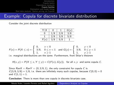
IntroductionCopula basics
Dependence measuresCopula families
Estimation and model fittingReal data analysis: Option pricing via Copulas
Example: Copula for discrete bivariate distribution
Consider the joint discrete distribution
Y\X 0 1 G(y)0 1/8 2/8 3/81 2/8 3/8 5/8
F (x) 3/8 5/8 1
F (x) = P(X ≤ x) =
0, x < 03/8, 0 ≤ x < 11, x ≥ 1
and G(y) =
0, y < 03/8, 0 ≤ y < 11, y ≥ 1
i.e. marginal distributions are the same. Furthermore, from Sklar’s theorem
H(x , y) = P(X ≤ x ,Y ≤ y) = C(F (x),G(y)), for all x , y and some copula C .
Since RanX = RanY = {0, 3/8, 1}, the only constraint for copula C isC(3/8, 3/8) = 1/8, i.e. there are infinitely many such copulas, because C(0, 0) = 0and C(1, 1) = 1.
Conclusion: There is more than one copula in discrete bivariate case.
Nikolai Kolev, Leandro Ferreira and Rafael Aguilera Dependence Analysis via Copulas

IntroductionCopula basics
Dependence measuresCopula families
Estimation and model fittingReal data analysis: Option pricing via Copulas
As conclusions for copula pitfalls
Any bivariate distribution with H(x , y) = P(X ≤ x ,Y ≤ y) can betrasformed to copula via
C(u, v) = H(F−1(u),G−1(v)), u, v ∈ [0, 1]. (2)
Thus, copula C represents the class of all bivariate distributions
H = [H(x , y)| continuous marginals are exactly F (x) and G(y)] .
In general, any result valid for bivariate distributions can be transportedto copula theory via (2).
But any result obtained for a copula
C(u, v) = P(U ≤ u,V ≤ v), U ∼ U(0, 1),V ∼ U(0, 1),
can be translated only for bivariate distributions E(x , y) with samemarginals (i.e. for exchangeable variables)
E(x , y) = P(X ≤ x ,Y ≤ y), with E(x ,∞) = F (x) and E(∞, y) = G(y).
Nikolai Kolev, Leandro Ferreira and Rafael Aguilera Dependence Analysis via Copulas
IntroductionCopula basics
Dependence measuresCopula families
Estimation and model fittingReal data analysis: Option pricing via Copulas
Parameter estimation
We will present three different methodologies (two parametricand one semi-parametric) to estimate unknown parameters:
The classical maximum likelihood estimation;
The inference for the marginals;
Semi-parametric approach, see Genest et al. (1995).
Observation: Exist Bayesian based approaches as well.
Nikolai Kolev, Leandro Ferreira and Rafael Aguilera Dependence Analysis via Copulas

IntroductionCopula basics
Dependence measuresCopula families
Estimation and model fittingReal data analysis: Option pricing via Copulas
Maximum likelihood estimation
To apply the maximum likelihood (ML) methodology, weneed to find the joint density in terms of the copula density.We have already seen that
h(x , y ; Θ) = c(F (x ; θ1),G (y ; θ2); θ)f (x ; θ1)g(y : θ2),
where θ1 and θ2 are parameters of the marginal distributionsand θ is copula parameter.
Therefore, Θ = (θ1, θ2, θ) is the parameter vector.
Nikolai Kolev, Leandro Ferreira and Rafael Aguilera Dependence Analysis via Copulas
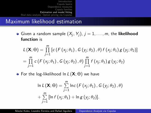
IntroductionCopula basics
Dependence measuresCopula families
Estimation and model fittingReal data analysis: Option pricing via Copulas
Maximum likelihood estimation
Given a random sample (Xj ,Yj), j = 1, . . . ,m, the likelihoodfunction is
L (X; Θ) =m∏j=1
[c (F (xj ; θ1) ,G (yj ; θ2) , θ) f (xj ; θ1) g (yj ; θ2)]
=m∏j=1
c (F (xj ; θ1) ,G (yj ; θ2) , θ)m∏j=1
f (xj ; θ1) g (yj ; θ2)
For the log-likelihood ln L (X; Θ) we have
ln L (X; Θ) =m∑j=1
lnc (F (xj ; θ1) ,G (yj ; θ2) , θ)
+m∑j=1
[ln f (xj ; θ1) + ln g (yj ; θ2)].
Nikolai Kolev, Leandro Ferreira and Rafael Aguilera Dependence Analysis via Copulas

IntroductionCopula basics
Dependence measuresCopula families
Estimation and model fittingReal data analysis: Option pricing via Copulas
Maximum likelihood estimation
Maximum likelihood estimators
The Maximum likelihood estimators are given by
θ = arg maxm∑j=1
∂ ln c (F (xj ; θ1)G (yj ; θn) , θ)
∂θ,
θ1 = arg maxm∑j=1
∂ ln c(F(xj ;θ1)G(yj ;θn),θ)∂θ1
+m∑j=1
∂ ln f (xj ;θ1)∂θ1
,
θ2 = arg maxm∑j=1
∂ ln c(F(xj ;θ1)G(yj ;θn),θ)∂θ2
+m∑j=1
∂ ln g(yj ;θ2)∂θ2
.
In general, we do not have closed form expressions for theparameter estimators, so numerical optimization is needed.
Nikolai Kolev, Leandro Ferreira and Rafael Aguilera Dependence Analysis via Copulas

IntroductionCopula basics
Dependence measuresCopula families
Estimation and model fittingReal data analysis: Option pricing via Copulas
Simulation of data set
Let us assume that marginals are Gamma distributed with parameters(α1, β1) = (2, 1) and (α2, β2) = (3, 2), i.e., the corresponding density function is
g(x ;α, β) =βαxα−1e−xβ
Γ(α)for x ≥ 0 and α, β > 0.
We will generate a sample of size n=200 of a bivariate distribution withselected Gamma marginals and Gaussian copula with parameter ρ = 0.5 usingR package copula, see Yan (2007).
1 l i b r a r y ( c o p u l a )23 myMvd = mvdc ( c o p u l a = e l l i p C o p u l a ( f a m i l y = ” normal ” , param = 0 . 5 ) , marg ins
= c ( ”gamma” , ”gamma” ) , paramMargins = l i s t ( l i s t ( shape = 2 , s c a l e =1) , l i s t ( shape = 3 , s c a l e = 2) ) )
4 n = 2005 dat = rmvdc (myMvd , n )6 p e r s p (myMvd , dMvdc , x l i m=c ( 0 , 1 ) , y l i m=c ( 0 , 1 ) , x l a b=” x1 ” , y l a b=” x2 ” , z l a b=” f
( x1 , x2 ) ” )7 p l o t ( dat [ , 1 ] , dat [ , 2 ] , x l a b=” x1 ” , y l a b=” x2 ” )89 u=pgamma( dat [ , 1 ] , shape = 2 , s c a l e = 1)
10 v=pgamma( dat [ , 2 ] , shape = 3 , s c a l e = 2)1112 p l o t ( u , v , x l a b=”U” , y l a b=”V” )
Nikolai Kolev, Leandro Ferreira and Rafael Aguilera Dependence Analysis via Copulas

IntroductionCopula basics
Dependence measuresCopula families
Estimation and model fittingReal data analysis: Option pricing via Copulas
Simulated data
Density of Simulated data
Nikolai Kolev, Leandro Ferreira and Rafael Aguilera Dependence Analysis via Copulas

IntroductionCopula basics
Dependence measuresCopula families
Estimation and model fittingReal data analysis: Option pricing via Copulas
Simulated data
Scatterplots of Simulated data and its Copula
Nikolai Kolev, Leandro Ferreira and Rafael Aguilera Dependence Analysis via Copulas
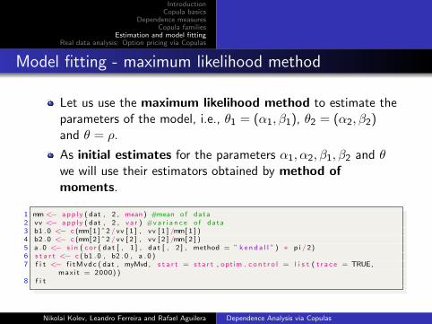
IntroductionCopula basics
Dependence measuresCopula families
Estimation and model fittingReal data analysis: Option pricing via Copulas
Model fitting - maximum likelihood method
Let us use the maximum likelihood method to estimate theparameters of the model, i.e., θ1 = (α1, β1), θ2 = (α2, β2)and θ = ρ.
As initial estimates for the parameters α1, α2, β1, β2 and θwe will use their estimators obtained by method ofmoments.
1 mm<− a p p l y ( dat , 2 , mean ) #mean o f data2 vv <− a p p l y ( dat , 2 , v a r ) #v a r i a n c e o f data3 b1 . 0 <− c (mm[ 1 ] ˆ 2 / vv [ 1 ] , vv [ 1 ] /mm[ 1 ] )4 b2 . 0 <− c (mm[ 2 ] ˆ 2 / vv [ 2 ] , vv [ 2 ] /mm[ 2 ] )5 a . 0 <− s i n ( c o r ( dat [ , 1 ] , dat [ , 2 ] , method = ” k e n d a l l ” ) ∗ p i / 2)6 s t a r t <− c ( b1 . 0 , b2 . 0 , a . 0 )7 f i t <− f i t M v d c ( dat , myMvd , s t a r t = s t a r t , opt im . c o n t r o l = l i s t ( t r a c e = TRUE,
maxi t = 2000) )8 f i t
Nikolai Kolev, Leandro Ferreira and Rafael Aguilera Dependence Analysis via Copulas

IntroductionCopula basics
Dependence measuresCopula families
Estimation and model fittingReal data analysis: Option pricing via Copulas
Results - maximum likelihood estimates
True values are: (α1, β1) = (2, 1), (α2, β2) = (3, 2) andρ = 0, 5.
The Maximum Likelihood estimation is based on 200 observations.
Marginal 1Estimate Std. Error
α1 2,046 0,190β1 1,034 0,109
Marginal 2Estimate Std. Error
α2 3,048 0,290β2 2,003 0,207
CopulaEstimate Std. Error
ρ 0,522 0,051
The maximized loglikelihood shows value -774,236
Nikolai Kolev, Leandro Ferreira and Rafael Aguilera Dependence Analysis via Copulas

IntroductionCopula basics
Dependence measuresCopula families
Estimation and model fittingReal data analysis: Option pricing via Copulas
Comments
Usually, the estimator of the copula dependence parameter θ isaffected by the parametric structure of the marginal distributions,i.e. by parameters θ1 and θ2. One can observe the inverse effectas well.
When we are interested mainly on the dependence structure, itis profitable to have a tool that relax this influence.
Two appropriate methodologies are
- the inference for the marginals;
- the semi-parametric method (when the marginal distributions areestimated using some non-parametric approach);
Both methods are conceptually straightforward.
Nikolai Kolev, Leandro Ferreira and Rafael Aguilera Dependence Analysis via Copulas
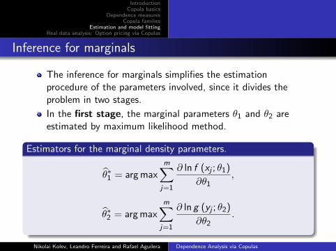
IntroductionCopula basics
Dependence measuresCopula families
Estimation and model fittingReal data analysis: Option pricing via Copulas
Inference for marginals
The inference for marginals simplifies the estimationprocedure of the parameters involved, since it divides theproblem in two stages.
In the first stage, the marginal parameters θ1 and θ2 areestimated by maximum likelihood method.
Estimators for the marginal density parameters.
θ∗1 = arg maxm∑j=1
∂ ln f (xj ; θ1)
∂θ1,
θ∗2 = arg maxm∑j=1
∂ ln g (yj ; θ2)
∂θ2.
Nikolai Kolev, Leandro Ferreira and Rafael Aguilera Dependence Analysis via Copulas

IntroductionCopula basics
Dependence measuresCopula families
Estimation and model fittingReal data analysis: Option pricing via Copulas
Inference for marginals
In the second stage, the dependence parameter θ isestimated using a pseudo-likelihood.
Dependence parameter estimator.
θ∗ = arg maxm∑j=1
∂ ln c (uj , vj , θ)
∂θ,
where uj = F(xj ; θ
∗1
), vj = G
(yj ; θ
∗2
)for all j = 1, . . . ,m.
The name pseudo-likelihood comes from the fact that we
use uj = F(xj ; θ
∗1
)and vj = G
(yj ; θ
∗2
)instead of the
observed values uj and vj , j = 1, . . . ,m.
Nikolai Kolev, Leandro Ferreira and Rafael Aguilera Dependence Analysis via Copulas

IntroductionCopula basics
Dependence measuresCopula families
Estimation and model fittingReal data analysis: Option pricing via Copulas
Clayton, Frank and Gaussian copulas
Let us apply the inference for marginals method toestimate the parameters of Clayton, Frank and Gaussiancopula joining the marginal gamma distributions.
1 #l o g l i k e l i h o o d f o r marg ins2 l o g l i k . marg <− f u n c t i o n ( b , x ) sum (dgamma( x , shape = b [ 1 ] , s c a l e = b [ 2 ] , l o g =
TRUE) )3 c t r l <− l i s t ( f n s c a l e = −1)45 #F i r s t s t a g e f o r e s t i m a t i o n p r o c e s s6 b1hat <− optim ( b1 . 0 , f n = l o g l i k . marg , x = dat [ , 1 ] , c o n t r o l = c t r l ) $ par7 b2hat <− optim ( b2 . 0 , f n = l o g l i k . marg , x = dat [ , 2 ] , c o n t r o l = c t r l ) $ par8 udat <− c b i n d (pgamma( dat [ , 1 ] , shape = b1hat [ 1 ] , s c a l e = b1hat [ 2 ] ) ,pgamma( dat [ ,
2 ] , shape = b2hat [ 1 ] , s c a l e = b2hat [ 2 ] ) )
Nikolai Kolev, Leandro Ferreira and Rafael Aguilera Dependence Analysis via Copulas

IntroductionCopula basics
Dependence measuresCopula families
Estimation and model fittingReal data analysis: Option pricing via Copulas
Inference for marginals
1 #second s t a g e f o r e s t i m a t i o n p r o c e s s2 #D e f i n i n g c o p u l a o b j e c t3 myCop . c l a y t o n <− c l a y t o n C o p u l a ( dim=2, param = 2)4 myCop . f r a n k <− f r a n k C o p u l a ( dim=2, param = 2)5 myCop . g a u s s i a n <− normalCopula ( dim=2, param = 0 . 9 )67 #Model f i t t i n g8 f i t . i f 1 <− f i t C o p u l a ( myCop . c l a y t o n , udat , s t a r t = a . 0 )9 f i t . i f 2 <− f i t C o p u l a ( myCop . f r a n k , udat , s t a r t = a . 0 )
10 f i t . i f 3 <− f i t C o p u l a ( myCop . g a u s s i a n , udat , s t a r t = a . 0 )
Nikolai Kolev, Leandro Ferreira and Rafael Aguilera Dependence Analysis via Copulas

IntroductionCopula basics
Dependence measuresCopula families
Estimation and model fittingReal data analysis: Option pricing via Copulas
Results - inference for marginals
The estimators of copula parameters using the inference formarginals method are:
Estimate Std. Error z value Pr(> |z |)Clayton param 0,644 0,127 5,061 4,17E-07
Frank param 2,964 0,499 5,945 2,76E-09Gaussian ρ 0,452 0,060 7,541 4,66E-14
ML of ρ was 0.522 (the true value in Gaussian case is 0.5)
How can we select the model that best fits the data?
Nikolai Kolev, Leandro Ferreira and Rafael Aguilera Dependence Analysis via Copulas

IntroductionCopula basics
Dependence measuresCopula families
Estimation and model fittingReal data analysis: Option pricing via Copulas
Inference for marginals - comments
The estimator of copula parameter θ obtained from themaximum likelihood and the inference for marginals methodsare different (0,522 and 0,452 in Gaussian case).
Xu (1996) performed Monte Carlo simulations to compare theresults and verified that in almost all simulations therelative efficiency was very close to 1.
In general, the inference for marginals method ispreferable than the exact maximum likelihood approach.
Nikolai Kolev, Leandro Ferreira and Rafael Aguilera Dependence Analysis via Copulas

IntroductionCopula basics
Dependence measuresCopula families
Estimation and model fittingReal data analysis: Option pricing via Copulas
Inference for marginals - comments
The estimation of the parameters in two steps leads to a lossin efficiency and standard errors cannot be obtained asthe inverse of the Fisher Information.
Patton (2006a) shows in a simulation study that method doesnot perform very well applying one step of theNewton-Rhapson algorithm to the full likelihood function.
Alternatively when the marginal model is unknown Genestet al. (1995) suggest modeling the marginal distribution withthe empirical distribution and estimating the copula via ranksof the data.
Nikolai Kolev, Leandro Ferreira and Rafael Aguilera Dependence Analysis via Copulas

IntroductionCopula basics
Dependence measuresCopula families
Estimation and model fittingReal data analysis: Option pricing via Copulas
Model selection
A general criteria for model selection is the AkaikeInformation Criterion (AIC ).
It was developed by Hirotsugu Akaike (Akaike, 1974) and isbased in the concept of information entropy, offering arelative measure of the information lost when somemodel is used to describe the reality.
Nikolai Kolev, Leandro Ferreira and Rafael Aguilera Dependence Analysis via Copulas
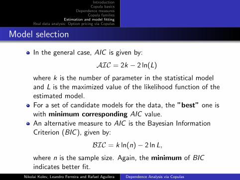
IntroductionCopula basics
Dependence measuresCopula families
Estimation and model fittingReal data analysis: Option pricing via Copulas
Model selection
In the general case, AIC is given by:
AIC = 2k − 2 ln(L)
where k is the number of parameter in the statistical modeland L is the maximized value of the likelihood function of theestimated model.
For a set of candidate models for the data, the ”best” one iswith minimum corresponding AIC value.
An alternative measure to AIC is the Bayesian InformationCriterion (BIC ), given by:
BIC = k ln(n)− 2 ln L,
where n is the sample size. Again, the minimum of BICindicates better fit.
Nikolai Kolev, Leandro Ferreira and Rafael Aguilera Dependence Analysis via Copulas

IntroductionCopula basics
Dependence measuresCopula families
Estimation and model fittingReal data analysis: Option pricing via Copulas
Inference for marginals
Below we present the code in R to obtain results applyingAIC and BIC criteria
1 #Aic c r i t e r i o n2 a i c C l a y t o n <− −2∗ f i t . i f 1 @ l o g l i k +23 a i c F r a n k <− −2∗ f i t . i f 2 @ l o g l i k +24 a i c G a u s s i a n <− −2∗ f i t . i f 3 @ l o g l i k +256 #Bic c r i t e r i o n7 b i c C l a y t o n <− −2∗ f i t . i f 1 @ l o g l i k+l o g ( 2 0 0 )8 b i c F r a n k <− −2∗ f i t . i f 2 @ l o g l i k+l o g ( 2 0 0 )9 b i c G a u s s i a n <− −2∗ f i t . i f 3 @ l o g l i k+l o g ( 2 0 0 )
Nikolai Kolev, Leandro Ferreira and Rafael Aguilera Dependence Analysis via Copulas

IntroductionCopula basics
Dependence measuresCopula families
Estimation and model fittingReal data analysis: Option pricing via Copulas
Model selection - inference for marginals method
Comparison among the models obtained by the inference formargins method.
Maximized LogL AIC BIC
Clayton 16,36 -30,73 -27,43Frank 22,08 -42,16 -38,86
Gaussian 22,74 -43,48 -40,18
i.e. the Gaussian copula gives better fit.
Nikolai Kolev, Leandro Ferreira and Rafael Aguilera Dependence Analysis via Copulas

IntroductionCopula basics
Dependence measuresCopula families
Estimation and model fittingReal data analysis: Option pricing via Copulas
Semi-parametric inference
Many semi-parametric methods can be found in theliterature, e.g., Clayton (1978), Clayton and Cuzick (1985),Genest et al. (1995) and Oakes (1994).
In all these approaches, the first step consists in estimating
the marginal distribution functions(F (x) , G (y)
)applying
some non-parametric methodology and, in the second step,performing a data transformation x1 y1
......
xm ym
(F (xj) G (yj)
)−→
u1 v1...
...um vm
.
In the third step, some parametric copula family that betterfits the data is chosen.
Nikolai Kolev, Leandro Ferreira and Rafael Aguilera Dependence Analysis via Copulas

IntroductionCopula basics
Dependence measuresCopula families
Estimation and model fittingReal data analysis: Option pricing via Copulas
Marginal distribution estimation
Several semi-parametric methodologies to estimate adensity function f (x) exist. For example, one can use kernelsmoothing to obtain f (x) and to calculate
F (x) =
∫f (x) dx .
In Genest et al. (1995), empirical distribution functionswere used,
F (xj) =rX ,j
m + 1, G (yj) =
rY ,jm + 1
,
where rX ,j is the rank of jth sample observation of randomvariable X (the same for Y ).
Nikolai Kolev, Leandro Ferreira and Rafael Aguilera Dependence Analysis via Copulas

IntroductionCopula basics
Dependence measuresCopula families
Estimation and model fittingReal data analysis: Option pricing via Copulas
Dependence parameter estimation
The dependence parameter can be estimated via
θ = arg maxm∑j=1
∂ ln c (uj , vj , θ)
∂θ.
The estimator θ is consistent and asymptotically normaldistributed.
Nikolai Kolev, Leandro Ferreira and Rafael Aguilera Dependence Analysis via Copulas

IntroductionCopula basics
Dependence measuresCopula families
Estimation and model fittingReal data analysis: Option pricing via Copulas
Semi-parametric inference
Below we present the code in R used to perform thesemi-parametric inference:
1 #F i r s t s t a g e : G e t t i n g e m p i r i c a l d i s t r i b u t i o n2 eu <− c b i n d ( ( rank ( dat [ , 1 ] ) − 0 . 5 ) /n , ( rank ( dat [ , 2 ] ) − 0 . 5 ) /n )34 #second s t a g e f o r e s t i m a t i o n p r o c e s s5 #D e f i n i n g c o p u l a o b j e c t6 myCop . c l a y t o n <− c l a y t o n C o p u l a ( dim=2, param = 2)7 myCop . f r a n k <− f r a n k C o p u l a ( dim=2, param = 2)8 myCop . g a u s s i a n <− normalCopula ( dim=2, param = 0 . 9 )9
10 #Model f i t t i n g11 f i t . cm1 <− f i t C o p u l a ( myCop . c l a y t o n , eu , s t a r t = a . 0 )12 f i t . cm2 <− f i t C o p u l a ( myCop . f r a n k , eu , s t a r t = a . 0 )13 f i t . cm3 <− f i t C o p u l a ( myCop . g a u s s i a n , eu , s t a r t = a . 0 )
Nikolai Kolev, Leandro Ferreira and Rafael Aguilera Dependence Analysis via Copulas

IntroductionCopula basics
Dependence measuresCopula families
Estimation and model fittingReal data analysis: Option pricing via Copulas
Semi-parametric inference
Below we present the code in R to obtain results applying AICand BIC criteria
1 #Aic c r i t e r i o n2 a i c C l a y t o n <− −2∗ f i t . c m 1 @ l o g l i k+23 a i c F r a n k <− −2∗ f i t . c m 2 @ l o g l i k+24 a i c G a u s s i a n <− −2∗ f i t . c m 3 @ l o g l i k+256 #Bic c r i t e r i o n7 b i c C l a y t o n <− −2∗ f i t . c m 1 @ l o g l i k+l o g ( 2 0 0 )8 b i c F r a n k <− −2∗ f i t . c m 2 @ l o g l i k+l o g ( 2 0 0 )9 b i c G a u s s i a n <− −2∗ f i t . c m 3 @ l o g l i k+l o g ( 2 0 0 )
Nikolai Kolev, Leandro Ferreira and Rafael Aguilera Dependence Analysis via Copulas

IntroductionCopula basics
Dependence measuresCopula families
Estimation and model fittingReal data analysis: Option pricing via Copulas
Semi-parametric inference
In the table below we present the results for the selected modelsusing the semi-parametric inference method.
Estimate Std. Error z value Pr(> |z |)Clayton param 0,503 0,102 4,940 7,82E-07
Frank param 2,894 0,508 5,699 1,21E-08Gaussian ρ 0,447 0,060 7,402 1,34E-13
For comparison, see inference for marginals results
Estimate Std. Error z value Pr(> |z |)Clayton param 0,644 0,127 5,061 4,17E-07
Frank param 2,964 0,499 5,945 2,76E-09Gaussian ρ 0,452 0,060 7,541 4,66E-14
Nikolai Kolev, Leandro Ferreira and Rafael Aguilera Dependence Analysis via Copulas

IntroductionCopula basics
Dependence measuresCopula families
Estimation and model fittingReal data analysis: Option pricing via Copulas
Semi-parametric inference: model selection
In the table below we present a comparison among the modelsusing AIC and BIC criterion.
Maximized LogL AIC BIC
Clayton 13,23 -24,46 -21,16Frank 21,19 -40,39 -37,09
Gaussian 33,07 -42,09 -38,80
For comparison (inference for marginals method)
Maximized LogL AIC BIC
Clayton 16,36 -30,73 -27,43Frank 22,08 -42,16 -38,86
Gaussian 22,74 -43,48 -40,18
Nikolai Kolev, Leandro Ferreira and Rafael Aguilera Dependence Analysis via Copulas

IntroductionCopula basics
Dependence measuresCopula families
Estimation and model fittingReal data analysis: Option pricing via Copulas
Real data analysis
Consider the bivariate stochastic process {Xt}Tt=1 withXt = (X1t ,X2t)
′. Let H(x1t , x2t) be the joint distribution. Whereas
F (x1t,θ1 ),G (x2t,θ2 ) the marginal distribution functions andf (x1t,θ1 ), g(x2t,θ2 ) the correponding density functions.By Sklar’s theorem there exists a copula functionC (·, ·|θ) : [0, 1]2 −→ [0, 1] mapping the marginal distributions of X1t andX2t to their joint distribution through
H(x1t , x2t) = C (F (x1t,θ1 ),G (x2t,θ2 )|θ).
To satisfy all this (theorical) requirement implies that we limit
ourselves to the specific case that each processes {Xit} only depends
on its own past, but not on the past of the other process
{Xjt , (i 6= j)}, and that there is only instantaneous causality between
the variables (described by copula).
Nikolai Kolev, Leandro Ferreira and Rafael Aguilera Dependence Analysis via Copulas

IntroductionCopula basics
Dependence measuresCopula families
Estimation and model fittingReal data analysis: Option pricing via Copulas
We assume that the marginals can be modeled parametrically.The probability integral transform of marginal distributions aregiven by Ut = F (x1t ; θ1) and Vt = G (x2t ; θ2) where θ1 and θ2 arethe vector of parameters. In financial econometrics Xit the marginalprocesses (i = 1, 2) are usually modeled by ARMA-GARCH typemodel, whose residuals are treated as independent andidentically distributed (i.i.d.) random variables.
Nikolai Kolev, Leandro Ferreira and Rafael Aguilera Dependence Analysis via Copulas

IntroductionCopula basics
Dependence measuresCopula families
Estimation and model fittingReal data analysis: Option pricing via Copulas
Fair rainbow options
Options consisting of two or more underlying stocks are called rainbow options. Theprice of these options are influenced by the dependence structure between the stockssince the fair option price still is the expected value.
Fair price of a bivariate rainbow option V (t,S1, S2)
Let S1 and S2 be two stocks traded on a complete and arbitrage free market. Let t bethe present time and T the time of maturity, then the price V (t, S1, S2) of an optionwith a given payoff function g(S1(T ), S2(T )) is
V (t, S1, S2) = exp{−r(T − t)}∫ ∞
0
∫ ∞0
g(x , y)f QS1,S2(x , y) dxdy .
Where f QS1,S2is the joint probability distribution of the two stocks under the
risk-neutral probability measure Q and the sigma-algebra Ft is the filtrationcontaining all information about the two stocks up to time t.
We will use in our analysis the so called Exchange option., i.e, the payoff function isgiven by g(S1(T ), S2(T )) = max(S2(T )− S1(T ), 0). This means that the option willbe exercised only if stock 2 is worth more than stock 1
Nikolai Kolev, Leandro Ferreira and Rafael Aguilera Dependence Analysis via Copulas

IntroductionCopula basics
Dependence measuresCopula families
Estimation and model fittingReal data analysis: Option pricing via Copulas
Real data analysis: Option pricing via Copulas
We use the observed data for 2 stocks to obtain a fairrainbow option price:
1 The food processing company Kraft Foods (KFT),representing {X1t};
2 The technology company Hewlett-Packard (HPQ),representing {X2t}.
KFT and HPQ are traded on the New York Stock Exchange.
We will analyse a one year time period from 1 August 2012 to30 September 2013 (250 trading days). We use daily closeprices (Pit) in USD that are adjusted for dividends and splits.
The LogReturn of individual series is given by
Rit = log(Pit)− log(Pi(t−1)), t = 1, 2, . . . , n = 249.
where Pit is the stock price at time t with i = 1, 2.
Nikolai Kolev, Leandro Ferreira and Rafael Aguilera Dependence Analysis via Copulas

IntroductionCopula basics
Dependence measuresCopula families
Estimation and model fittingReal data analysis: Option pricing via Copulas
KFT and HPQ: Stock prices and LogReturns
Daily stock prices and LogReturns for KFT (above) and HPQ (below) over the sample period.
First deductions:
1 The LogReturns range of KFT is more volatile that HPQ;
2 It is not evident if both series are independent or dependent.
Nikolai Kolev, Leandro Ferreira and Rafael Aguilera Dependence Analysis via Copulas

IntroductionCopula basics
Dependence measuresCopula families
Estimation and model fittingReal data analysis: Option pricing via Copulas
KFT and HPQ: Histograms
Histograms of the LogReturns for KFT and HPQ.
Nikolai Kolev, Leandro Ferreira and Rafael Aguilera Dependence Analysis via Copulas

IntroductionCopula basics
Dependence measuresCopula families
Estimation and model fittingReal data analysis: Option pricing via Copulas
KFT and HPQ: Dependence Analysis
To test independence between LogReturns of KFT and HPQ we use thefollowing statistics
- for correlation coefficient: ρn√n−1∼ N(0, 1), where ρn is sample Pearson’s;
- for Kendall’s tau:√
92n(n−1)2n+5
τn ∼ N(0, 1), where τn is sample Kendall’s.
In table below several calculus values of measures of dependence between theLogReturns of KFT and HPQ are displayed along with corresponding p-valuesfor the null hypothesis of independence.
Spearman’s rho Kendall’s tau Correl. coef.0.206 0.139 0.153
p-value 0.0053 0.0052 0.008Measures of dependence between LogReturns of KFT and LogReturns of HPQ.
Conclusion: The KFT and HPQ stocks are statistically dependent (of level 0.8%).
Nikolai Kolev, Leandro Ferreira and Rafael Aguilera Dependence Analysis via Copulas
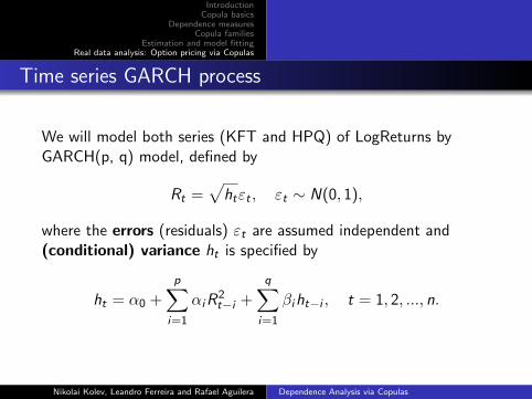
IntroductionCopula basics
Dependence measuresCopula families
Estimation and model fittingReal data analysis: Option pricing via Copulas
Time series GARCH process
We will model both series (KFT and HPQ) of LogReturns byGARCH(p, q) model, defined by
Rt =√
htεt , εt ∼ N(0, 1),
where the errors (residuals) εt are assumed independent and(conditional) variance ht is specified by
ht = α0 +
p∑i=1
αiR2t−i +
q∑i=1
βiht−i , t = 1, 2, ..., n.
Nikolai Kolev, Leandro Ferreira and Rafael Aguilera Dependence Analysis via Copulas
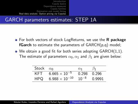
IntroductionCopula basics
Dependence measuresCopula families
Estimation and model fittingReal data analysis: Option pricing via Copulas
GARCH parameters estimates: STEP 1A
For both vectors of stock LogReturns, we use the R packagefGarch to estimate the parameters of GARCH(p,q) model;
We obtain a good fit for both series adopting GARCH(1,1).The estimate of parameters α0, α1 and β1 are given below:
Stock α0 α1 β1
KFT 6.665× 10⁻⁵ 0.298 0.296HPQ 6.988× 10⁻¹⁰ 10−8 0.9991
Nikolai Kolev, Leandro Ferreira and Rafael Aguilera Dependence Analysis via Copulas
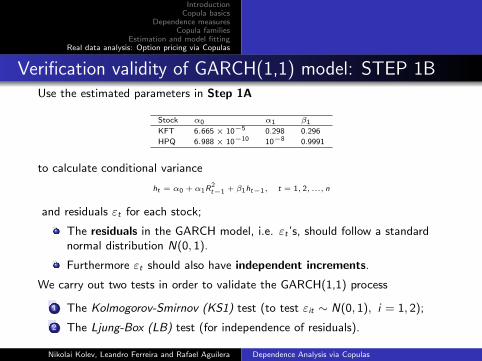
IntroductionCopula basics
Dependence measuresCopula families
Estimation and model fittingReal data analysis: Option pricing via Copulas
Verification validity of GARCH(1,1) model: STEP 1BUse the estimated parameters in Step 1A
Stock α0 α1 β1
KFT 6.665× 10⁻⁵ 0.298 0.296
HPQ 6.988× 10⁻¹⁰ 10−8 0.9991
to calculate conditional variance
ht = α0 + α1R2t−1 + β1ht−1, t = 1, 2, ..., n
and residuals εt for each stock;
The residuals in the GARCH model, i.e. εt ’s, should follow a standardnormal distribution N(0, 1).
Furthermore εt should also have independent increments.
We carry out two tests in order to validate the GARCH(1,1) process
1 The Kolmogorov-Smirnov (KS1) test (to test εit ∼ N(0, 1), i = 1, 2);
2 The Ljung-Box (LB) test (for independence of residuals).
Nikolai Kolev, Leandro Ferreira and Rafael Aguilera Dependence Analysis via Copulas

IntroductionCopula basics
Dependence measuresCopula families
Estimation and model fittingReal data analysis: Option pricing via Copulas
The Kolmogorov-Smirnov (KS1) test
The Kolmogorov-Smirnov (KS1) test is applied for each stocks residualεit , i = 1, 2 with a 5% significance level.
The residuals empirical distribution Femp(x) and Gemp(y) are used to checkN(0, 1) for residuals.
The statistical tests and p-values are presented below:
KS1 = maxx
(|Φ(x)−Femp(x)|) and KS1 = maxy
(|Φ(y)−Gemp(y)|), Φ(·) ∼ N(0, 1).
KFT HPQKS1 0.558 0.566p-value 0.888 0.872
The KS1 distance and p-values testing N(0, 1) of the residuals.
We can not reject the null hypothesis that residual are indeedstandard normally distributed.
Nikolai Kolev, Leandro Ferreira and Rafael Aguilera Dependence Analysis via Copulas

IntroductionCopula basics
Dependence measuresCopula families
Estimation and model fittingReal data analysis: Option pricing via Copulas
The Ljung-Box (LB) test
The increments independence of εit , i = 1, 2 is tested with the Ljung-Box (LB)test
LB = N(N + 2)M∑k=1
ρk
N − k∼ χ2(M),
where N is the sample size, M is the number of autocorrelation lags and
ρk =
∑ki=1(xi−x)(yi−y)√∑k
i=1(xi−x)2
√∑ki=1
(yi−y)2is the autocorrelation at lag k.
The null hypothesis is that there is no autocorrelation. For N(0, 1) residuals,this implies independent increments of εit , i = 1, 2. The results are givenbelow:
KFT HPQLB 19.243 7.860p-value 0.203 0.929
P-values for independence of the residuals using Ljung-Box test.
It can be seen, that we can not reject the null hypothesis that
residuals are independent, (i.e., there is no autocorrelation), at 5%
significance level.Nikolai Kolev, Leandro Ferreira and Rafael Aguilera Dependence Analysis via Copulas

IntroductionCopula basics
Dependence measuresCopula families
Estimation and model fittingReal data analysis: Option pricing via Copulas
QQ-Plot of Residuals
QQ-plot of Residuals for KFT and HPQ.
By now, we justified the choice of GARCH(1,1) model for KFT and HPQ.
Nikolai Kolev, Leandro Ferreira and Rafael Aguilera Dependence Analysis via Copulas
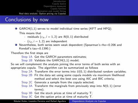
IntroductionCopula basics
Dependence measuresCopula families
Estimation and model fittingReal data analysis: Option pricing via Copulas
Conclusions by now
GARCH(1,1) serves to model individual time series (KFT and HPQ).
This means that- residuals (εit , i = 1, 2) are N(0, 1) distributed
- (εit , i = 1, 2) are independentNevertheless, both series seem weak dependent (Spearman’s rho=0.206 andKendall’s tau=0.1390.)
Therefore the first steps areStep 1A Get the GARCH parameters estimates;Step 1B Validate the GARCH(1,1) model;
So we will complement the analysis joining the error terms of both series with anappropriate copula. The algorithm can be summarized as follows
Step 2A Transform the error terms into U(0, 1) distributed random variables;Step 2B Fit the data set using some copula models via maximum likelihood
method and select the best one using AIC and BIC criteria;Step 2C Generate a sample from the copula selected;Step 3A Transform the marginals from previously step into N(0, 1) (error
terms);Step 3B Get the stock prices at time of maturity T;Step 3C Get the option price at time of maturity T.
Nikolai Kolev, Leandro Ferreira and Rafael Aguilera Dependence Analysis via Copulas

IntroductionCopula basics
Dependence measuresCopula families
Estimation and model fittingReal data analysis: Option pricing via Copulas
Transform the error terms into marginal uniforms: STEP2A
In order to use copulas to join residuals in both series, we need to transform the errorterms into U(0, 1) distributed random variables. We invert residuals εit obtained instep 1B for each stock into U(0, 1) by u = Φ(ε1i ) and v = Φ(ε2i ) , whereΦ(.) ∼ N(0, 1), i = 1, 2, ..., 249.
Scatterplot of copula jointly residuals of both series.Nikolai Kolev, Leandro Ferreira and Rafael Aguilera Dependence Analysis via Copulas

IntroductionCopula basics
Dependence measuresCopula families
Estimation and model fittingReal data analysis: Option pricing via Copulas
Copula fitting and model selection: STEP 2B
Apply the maximum likelihood to fit a copula to (u, v) from Step 2A. That is,for the transformed data {ut , vt}nt=1, estimate the copula parameters θC through
ArgMaxθC
n∑t=1
ln[c((ut , vt); θC )],
where c(u, v) is the density function of the selected copula C(u, v |θC ).
Copula Gaussian Student’s t Clayton Gumbel
Parameter 0.135 (0.139, 308.48) 0.028 1.059AIC -3.087 -0.976 1.567 0.562BIC 0.430 6.059 5.085 4.079
The estimated parameters for the different copulas and corresponding values of AIC and BIC criteria.
i.e. the Gaussian copula gives better fit.
Nikolai Kolev, Leandro Ferreira and Rafael Aguilera Dependence Analysis via Copulas

IntroductionCopula basics
Dependence measuresCopula families
Estimation and model fittingReal data analysis: Option pricing via Copulas
Generate a sample from the copula: STEP 2C
Generate a sample {u∗t , v∗t }Tt=1 from a U(0, 1) marginal distribution using the chosencopula. Here T is the time to maturity for the option;
Scatterplot of a sample {u∗t , v∗t }Tt=1 from a Gaussian copula.
Nikolai Kolev, Leandro Ferreira and Rafael Aguilera Dependence Analysis via Copulas

IntroductionCopula basics
Dependence measuresCopula families
Estimation and model fittingReal data analysis: Option pricing via Copulas
Transform the generated marginals into N(0,1) margins:STEP 3A
For each time instant t = 1, ...,T , transform the generatedmarginals into N(0,1) margins (in the risk-neutral world), byε∗1t = Φ−1(u∗t ) and ε∗2t = Φ−1(v∗t );
Histogram of Residuals for KFT and HPQ.Nikolai Kolev, Leandro Ferreira and Rafael Aguilera Dependence Analysis via Copulas

IntroductionCopula basics
Dependence measuresCopula families
Estimation and model fittingReal data analysis: Option pricing via Copulas
Stock price at time of maturity T: STEP 3B
Use ε∗it from Step 3A to calculate the conditional variances hitgive as considering GARCH parameters estimated in Step 1A.The two future stock prices at time T are
Si (T ) = Si (0) exp{ T∑
t=1
√hitε∗it
}, i = 1, 2;
Stock Price
KFT 44.95HPQ 17.50
Stock prices at maturity time T = 260 using Gaussian Copula (i.e. 10 days after our
last observations).
Nikolai Kolev, Leandro Ferreira and Rafael Aguilera Dependence Analysis via Copulas

IntroductionCopula basics
Dependence measuresCopula families
Estimation and model fittingReal data analysis: Option pricing via Copulas
Application: Monte Carlo integration using copulas
Aim: to obtain the expected value of a continuous functionq(x , y) of a bivariate random vector (X ,Y ) having jointdistribution H(x , y), i.e.
E (q(X ,Y )) =
∫ ∞y=−∞
∫ ∞x=−∞
q(x , y)dH(x , y);
Given the copula C (u, v) = H(F−1(v),G−1(v)) and marginaldistributions F (x) = lim
y→∞H(x , y) and G (y) = lim
x→∞H(x , y),
we can use the following algorithm to approximate the valueof E (q(X ,Y )):
1 generate n observations of the bivariate random vector (X ,Y );2 for each observation i , calculate qi = q(xi , yi ), i = 1, 2, ..., n;3 E (q(X ,Y )) ≈ 1
n
∑ni=1 qi
Nikolai Kolev, Leandro Ferreira and Rafael Aguilera Dependence Analysis via Copulas

IntroductionCopula basics
Dependence measuresCopula families
Estimation and model fittingReal data analysis: Option pricing via Copulas
Option price at time of maturity T: STEP 3C
Let g(S1(T ),S2(T )) = max(S2(T )− S1(T ), 0) be the payofffunction and repeat Steps 2C to 3B for N runs. Finally, weobtain the Monte Carlo option price:
V (t,S1, S2) =exp{−r(T − t)}
N
N∑i=1
g(S1i (T ),S2i (T )).
Exchange option 24.23
Option prices for Exchange option at time of maturity T=260.
Nikolai Kolev, Leandro Ferreira and Rafael Aguilera Dependence Analysis via Copulas

IntroductionCopula basics
Dependence measuresCopula families
Estimation and model fittingReal data analysis: Option pricing via Copulas
Comments
The marginal distributions that describe the individualbehavior of each variables and the copula that fully capturesthe dependence between the variables.
Furthermore, given a set of marginal distributions and acopula a multivariate distribution can be constructed bycoupling the marginals with the copula. The flexibility of theway dependencies can be modeled independently of themarginal distributions.
Nikolai Kolev, Leandro Ferreira and Rafael Aguilera Dependence Analysis via Copulas

IntroductionCopula basics
Dependence measuresCopula families
Estimation and model fittingReal data analysis: Option pricing via Copulas
Several conclusions
Copula is useful tool in many applied areas where the interest is inanalysis of multivariate dependence and when the multivariatenormal distribution is controversial.
In actuarial science, copulas are used in modeling dependencebetween mortality and losses, e.g., Frees, Carriere and Valdez(1996), Frees and Valdez (1998), Frees and Wang (2005).
In finance, copulas are successfully applied in asset allocation,credit scoring, default risk modeling, derivative pricing and riskmanagement, e.g., Bouye, Durrleman, Bikeghbali, Riboulet andRoncalli (2000), Embrechts, Lindskog and McNeil (2003) andCherubini, Luciano and Vecchiato (2004).
In biomedical studies, copulas are used in modeling correlated
events times and competing risks, e.g., Wang and Wells (2000),
Escarela and Carriere (2003).
Nikolai Kolev, Leandro Ferreira and Rafael Aguilera Dependence Analysis via Copulas

IntroductionCopula basics
Dependence measuresCopula families
Estimation and model fittingReal data analysis: Option pricing via Copulas
Several conclusions
In many real situations, empirical evidence has proved theinadequate use of the normal multivariate distribution:
Empirical marginal distributions are skewed and heavy-tailed;Possibilities of extreme co-movements, in contrast to themultivariate normal distribution.
Copulas provide an alternative solution and often more usefulrepresentations of multivariate distribution functionscompared to traditional approaches such as multivariatenormal distribution.
The use of linear correlation coefficient should be restricted tomultivariate elliptical distributions. Copula baseddependence measures (Spearman’s ρS and Kendall’s τK )are free of such limitations.
Nikolai Kolev, Leandro Ferreira and Rafael Aguilera Dependence Analysis via Copulas

IntroductionCopula basics
Dependence measuresCopula families
Estimation and model fittingReal data analysis: Option pricing via Copulas
References
Bouye, E., Durrleman, V., Bikeghbali, A., Riboulet, G. and Roncalli, T.(2000). Copulas for Finance - A Reading Guide and Some Applications.Working paper, Groupe de Recherche Operationnelle, Credit Lyonnais.
Blest, D. C.(2000). Rank correlation: an alternative measure. Australianand New Zealand Journal of Statistics, 42, 101-111.
Cherubini, U., Luciano, E. and Vecchiato, W. (2004). Copula Methods inFinance. John Wiley & Sons.
Embrechts, P., Lindskog, F. and McNeil, A. (2003). ModellingDependence with Copulas and Applications to Risk Management. In SRachev (ed.), Handbook of Heavy Tailed Distribution in Finance. pp.329-384. Elsevier.
Escarela, G. and Carriere, J.F. (2003). Fitting Competing Risks with anAssumed Copula. Statistical Methods in Medical Research 12, 333-349.
Frees, E.W, Carriere, J. and Valdez, E.A. (1996). Annuity Valuation withDependent Mortality. Journal of Risk and Insurance 63, 229-261.
Nikolai Kolev, Leandro Ferreira and Rafael Aguilera Dependence Analysis via Copulas

IntroductionCopula basics
Dependence measuresCopula families
Estimation and model fittingReal data analysis: Option pricing via Copulas
References
Frees, E.W. and Valdez, E.A. (1998). Understanding Relationships UsingCopulas. North American Actuarial Journal 2, 1-25.
Frees, E.W. and Wang, P. (2005). Credibility Using Copulas. NorthAmerican Actuarial Journal 9, 31-48.
Meucci, A. (2011). A short, comprehensive, practical guide to copulas.Garp Risk Professional, October, 22-27.
Sklar, A. (1959). Fonctions de repartition n dimensions et leurs marges.Publ Inst Statist Univ Paris 8, 229-231.
Wang, W. and Wells, M.T. (2000). Model Selection and SemiparametricInference for Bivariate Failure-time Data. Journal of the AmericanStatistical Association 95, 62-72.
Nikolai Kolev, Leandro Ferreira and Rafael Aguilera Dependence Analysis via Copulas

IntroductionCopula basics
Dependence measuresCopula families
Estimation and model fittingReal data analysis: Option pricing via Copulas
References
Akaike, H. (1974). A new look at the statistical modelidentification. IEEE Transactions on Automatic Control 19 716-723.
Clayton, D.G. (1978). A model for association in bivariate life tablesand its applications in epidemiological studies of familial tendency inchronic disease incidence. Biometrika 65, 141-151.
Clayton, D.G. and Cuzick, J. (1985). Multivariate generalizations ofthe proportional hazards model. Journal of Royal Statistics SocietyA 148, 82-117.
Fisher, N. and Switzer, P. (1985). Chi-plots for assessingdependence. Biometrika 72, 253-265.
Fisher, N. and Switzer, P. (2001). Graphical assessment ofdependence: is a picture worth 100 tests? The AmericanStatistician 55, 233-239.
Nikolai Kolev, Leandro Ferreira and Rafael Aguilera Dependence Analysis via Copulas

IntroductionCopula basics
Dependence measuresCopula families
Estimation and model fittingReal data analysis: Option pricing via Copulas
References
Frees, E.W. and Wang, P. (2005). Credibility Using Copulas. NorthAmerican Actuarial Journal 9, 31-48.
Genest, C. and Boies, J.C. (2003). Detecting dependence withKendall plots. The American Statistician 57, 275-284.
Genest, C., Ghoudi, K. and Rivest, L.P. (1995). A semiparametricestimation procedure of dependence paramaters in multivariatefamilies of distributions. Biometrika 82, 543-552.
McNeil, A., Frey, L. and Embrechts, P. (2005). Quantitative RiskManagement. Princeton University Press.
Oakes, D. (1994). Multivariate survival distributions. Journal ofNonparametric Statistics 3, 343-354.
Yan, J. (2007). Enjoy the joy of copulas: with a package copula.Journal of Statistical Software 21, 1-21.
Nikolai Kolev, Leandro Ferreira and Rafael Aguilera Dependence Analysis via Copulas