dependency equilibria and the causal structure of … · dependency equilibria and the causal...

Homo Oeconomicus XX(2/3) (ACCEDO Verlagsgesellschaft, München 2003)

Dependency Equilibria and the Causal Structure of Decision andGame Situations

byWolfgang Spohn'

Abstract: The paper attempts to rationalize cooperation in the one-shot prisoners' di-lemma (PD). It starts by introducing (and preliminarily investigating) a new kind ofequilibrium (differing from Aumann's correlated equilibria) according to which theplayers' actions may be correlated (sect. 2). In PD the Pareto-optimal among theseequilibria is joint cooperation. Since these equilibria seem to contradict causal precon-ceptions, the paper continues with a standard analysis of the causal structure of decisi-on situations (sect. 3). The analysis then raises to a reflexive point of view accordingto which the agent integrates his own present and future decision situations into thecausal picture of his situation (sect. 4). This reflexive structure is first applied to thetoxin puzzle and then to Newcomb's problem, showing a way to rationalize drinkingthe toxin and taking only one box without assuming causal mystery (sect. 5). The latterresult is finally extended to a rationalization of cooperation in PD (sect. 6).

Contents:

1. Introduction2. Dependency Equilibria

2.1 Nash, correlated and dependency equilibria2.2 Some examples2.3 Some observations

3. Causal Graphs, Bayesian Nets, Reductions, and Truncations3.1 Causal graphs and Bayesian nets3.2 Reductions of causal graphs and Bayesian nets3.3 Actions, truncations, and basic decision models

4. Reflexive Decision Theory4. t Dependency schemes and strategies4.2 Reflexion4.3 Reflexive decision models and their truncated reductions4.4 Where do we stand?

"Prof. Dr. Wolfgang Spohn, Fachbereich Philosophie, Universität Konstanz, D-78457 Konstanz,email; [email protected].

196 W. Spohn5. The Toxin Puzzle and Newcomb' s Problem

5.1 The toxin puzzle5.2 Newcomb's problem

6. Prisoners' Dilemma6.1 How cooperation may be rational in prisoners' dilemma6.2 A dialogue6.3 Some comparative remarks

References

1. Introduction'

The driving force behind this paper is, once more, the great riddle posed by theprisoners' dilemma (PD). This has elicited a vast literature and a large number ofastonishingly varied attempts to undermine defection as the only rational solution andto establish cooperation as a rational possibility at least in the iterated case. But thehard case, it seems to me, still stands unshaken. Under appropriate conditionsbackward induction is valid'; hence, given full rationality (instead of some form of'bounded rationality') and sufficient common knowledge, continued defection is theonly solution in the finitely iterated PD. The same conclusion is reached via theiterated elimination of weakly dominated strategies.2 I find this conclusion highlydisconcerting; it amounts to an outright refutation of the underlying theory ofrationality. Moreover, I find that all the sophisticated observations made so far about

'This paper was conceived and partially written during my stay at the Center for InterdisciplinaryResearch of the University of Bielefeld in the summer term 2000, where I participated in the researchgroup „Making Choices. An Interdisciplinary Approach to Modelling Decision Behaviour". I amgrateful to the Center and to the organizers of the group, Reinhard Selten, Werner Guth, HartmutKliemt, and Joachim Frohn, for the invitation, and I am indebted to all the participants of the researchgroup for the strong stimulation and encouragement 1 have experienced. Moreover, I am grateful toMax Albert, Robert Aumann, Christopher von Bulow, Werner Güth, Rainer Hegseimann, ArthurMerin, Matthias Risse, Jacob Rosenthal, Thomas Schmidt, and Yanis Varoufakis for comments onpreliminary drafts, to Philip Dawid for pointing out to,me a serious flaw in section 3.2 (which is nowrepaired in a satisfying way, I hope), to Adelheid Baker for meticulously checking my English, and toHartmut Kliemt for being indulgent with this overly long paper. In particular the rich comments byMax Albert, Matthias Risse, and Yanis Varoufakis have shown me the insufficiency of my paper. Thearrangement of the subject matter may be infelicitous in various respects, the comparative remarks insection 6.3 and throughout the text are too scarce in almost all respects. But clearly, the topic isinexhaustible, and the question is: how to live up to an inexhaustible topic? Only by coming to apreliminary end, none the less.'Cf. Aumann (1995).'Iterated elimination of weakly dominated strategies is a reasonable procedure when applied to theiterated PD, all the more so as the criticism this may meet compared to the elimination of stronglydominated strategies do not obtain in this application. Cf, e.g., Myerson (1991, sects. 2.5 and 3.1).

Dependency Equilibria 197PD have failed to tone down this harsh conclusion.3 Cooperation must remain at least arational possibility in the finitely iterated PD, and under ideal conditions even more sothan under less ideal ones." Thus, something needs to be changed in standardrationality theory, i.e., decision and game theory. After a long time of thinkingotherwise5,1 have come to the conclusion that it is the single-shot case that needs to bereconsidered, which this paper tries to do.

This is how my plot is supposed to go.' Section 2 introduces and discusses a newnotion of equilibrium for games in normal form which I call dependency equilibrium.In particular, mutual cooperation will be a dependency equilibrium in the single-shotPD. These equilibria may be an object of interest in their own right, but they seem toassume an unintelligible causal loop, namely, that the players' actions causallyinfluence each other (this may be why they have not been considered in the literature).Thus, my main effort in this paper will be to make causal sense of them; then and onlythen they deserve interest.

To this end, section 3 introduces some basics of the theory of causation that hasbecome standard and has been implicitly or explicitly assumed in decision and non-cooperative game theory since their inception. The crucial observation will be this(section 3.2): Whenever we reduce a richer causal model to a coarser one by deletingsome variables, each (apparent) causal dependence in the coarser model expresseseither a possibly indirect causal dependence or the relation of having a common causein the richer model (or a still more complicated relation which will turn out, though, tobe irrelevant for our concerns). Hence, the apparent mutual causal dependence of theactions in a dependency equilibrium may only signify that they have a common cause.

This will lead us to the question of how an action is caused. In rational decisiontheory the answer can only be that it is caused by the decision situation (= the agent'ssubjective state). Hence, if the causes of actions are to enter the causal picture of the

'As I have more fully explained in Spohn (2000, sect. 5)."Aumann's proof of backward induction assumes common knowledge of resilient rationality (CKR),i.e., the mutual belief that the players will behave rationally even after arbitrary deviations from therational equilibrium path. Aumann (1995, p. 18) grants that "CKR is an ideal condition that is rarelymet in practice" ("ideal" in the sense of "idealized"), and since this assumption looks implausibleeven as a rationally entertainable belief (cf. Rabinowicz 1998), one may hope to find a loophole here.I am skeptical, however. In actual life, I have certainly to reckon with the irrationality of my fellowhumans, but this should not be the only possibility how my repeated cooperation may turn out asrational. It should all the more prove as rational, given the most unshakeable mutual beliefs incommon rationality.'Since Spohn (1978, sect. 5.1) I have been a fervent defender of the two-box solution ofNewcomb'sproblem, but I have changed my mind (see sect. 5.2 below). In Spohn (2000, sect. 6) I have offered aline of thought for breaking the force of backward induction in the iterated case, but I amwithdrawing it since I do not see anymore how it can be reasonably worked out.'In case this summary is too abstract, it may at least serve as a reference.

198 W. Spohnagent, we have to develop standard decision theory to become what I call reflexivedecision theory (because the possible decision situations themselves are now reflectedin decision models). This is the task addressed in section 4, where the crucialobservation will be this: A decision situation (= the agent's subjective state) may haveother effects besides the action. If we now reduce the reflexive model to a standardnon-reflexive model, the action will appear to cause these other effects in the reducedmodel, though reflexion shows that they actually have only a common cause.

In section 5, this observation is applied to the toxin puzzle and to Newcomb'sproblem. This is suggested by the fact that these cases allow (though they do not force)us to conceive the agent's decision situation as having such side effects, i.e., assomehow causing the prediction of the relevant predictor. Thereby we can rationalizedrinking the toxin or taking only one box within causal decision theory in a perfectlystraightforward way. Having got thus far, I transfer this kind of analysis to the two-person case of PD where we may similarly conceive the decision situations of theplayers as being causally entangled. Thus, the dependency equilibria in PD with theirapparent causal loop in the actions acquire causal sense and may thus be rationalized.In this way, cooperation emerges at least as a rational possibility, and backwardinduction cannot even start. This is the task dealt with in section 6.1.

I will be mainly occupied with developing this line of thought in detail. However,a fictitious dialogue in section 6.2 and a number of comparative remarks in section 6.3will, I hope, further clarify the nature of my approach.

The paper borrows from many sources. But I should emphasize that, with regard tosection 4, my main debt is to Eells (1982) who was the first to take the reflexiveperspective in decision theory. In section 5, it will become obvious how strongly I aminfluenced by the theory of resolute choice developed by McClennen (1990). I hope toadvance it by showing how resolute choice may be subsumed under the reflexiveextension of standard rationality theory.

2. Dependency Equilibria

2.1 Nash, correlated and dependency equilibria

Let me start with an outline of the new equilibrium concept. For comparison, it isuseful to rehearse Nash equilibria and Aumann's correlated equilibria. We shall dealonly with normal form games. Hence, the refinements of Nash equilibria relating to theextensive form are out of our focus. It suffices to consider two-person games. While Ihardly develop the theory here, it may be routinely extended, it seems, to «-persongames.

Dependency Equilibria 199Thus, let A = {a\,...,am} be the set of pure strategies of Ann (row chooser) and B =

{b\,...,bn} the set of pure strategies of Bob (column chooser). Let u and v be the utilityfunctions of Ann and Bob, respectively, from A x B into R; we abbreviate un =u(ai, bic) and v,» = v(a,, bk).

Moreover, let S be the set of mixed strategies of Ann, i.e., the set of probabilitydistributions over A. Hence, s = (s],...,Sm) = (s,) e S iff s, 0 for ; = l,...,m andm^s,=l. Likewise, let T be. the set of mixed strategies of Bob. Mixed strategies have1=1an ambiguous interpretation. Usually, the probabilities are thought to be intentionalmixtures by each player. But it is equally appropriate to interpret them as representingthe beliefs of others about the player. Indeed, in relation to dependency equilibria, thiswill be the only meaningful interpretation.

We shall envisage the possibility that the actions in a game may be governed byany probability distribution whatsoever. Let P be the set of distributions over A x B.Thus, p = (pile) e P iffpjk^O for all i = \,...,m and k = l,...,n and ^p,k = 1. Each

i,k

p < = P has a marginal s over A and a marginal t over B. But since p may containarbitrary dependencies between A and B, it is usually not the product of the marginals sand /. This is all the terminology we shall need.

As is well known, (s, t) is defined as a Nash equilibrium iff for ally = l,...,mE^t"tt > E^t (OT' equivalently, for all s* e S E^"rt > Z-?,*'*";*) and if thei.k k . i,k i,k

corresponding condition holds for the other player. Hence, in a Nash equilibriumneither Ann nor Bob can raise her or his expected utility by changing from her or hisequilibrium strategy to some other pure or mixed strategy, given the other player sticksto his or her equilibrium strategy. There is no need here to rehearse the standardrationale for Nash equilibria, and there is no time to discuss its strengths andweaknesses.'

Obviously Ann and Bob's choices from A and B are independent in a Nashequilibrium. This is an assumption I would like to abandon (for reasons that willbecome clear later on). Aumann (1974) has introduced an equilibrium concept thatallows for dependence between the players. Here is his definition from Aumann(1987) (which is a little simpler and less general than his original definition whichwould require us to introduce additional structure):

Let p e P have marginals s e S and t e T. Then p is a correlated equilibrium ifffor ally = \,...,m ^P,k",k 2 ^t^jk (or' equivalently, for all s* e S ^P ik >-

i,k k i.k

^s^t^Ujk) and if the corresponding condition holds for the other player. The most',*

'This has been done many times, also by myself in Spohn (1982).

200 W. Spohnstraightforward way to understand this, which is offered by Aumann himself (1987,pp. 3f.), is the following: Somehow, Ann and Bob agree on a joint distribution over thestrategy combinations or outcomes of their game. One combination is chosen atrandom according to this distribution, and each player is told only their part of thecombination. If no player can raise their expected utility by breaking their part of theagreed joint distribution and choosing some other pure or mixed strategy instead, thenthis joint distribution is a correlated equilibrium. Thus, correlated equilibria are self-enforcing, they do not need external help from sanctions or agreements.

Correlated equilibria appear to fall outside non-cooperative game theory.However, one can model the selection of a joint distribution for the original game asan additional move in a game enlarged by preplay communication, and it then turns outthat all and only the Nash equilibria of the enlarged game correspond to correlatedequilibria in the original game.' This reflects the fact that correlated equilibria, despitetheir allowance of dependence, are still non-cooperative in essence. The players'standard of comparison is still whether they might be better off by independently doingsomething else, where the expectations about the other player are given by themarginal over their strategies.

This standard of comparison is changed in the dependency equilibria introducedbelow. It is not the expected utility given the marginal for the other player, but ratherthe conditional expected utility given the conditional probabilities determined by thejoint distribution.

Here is a first attempt to formalize this idea: Let p e P have marginals s e S and( e T. Let pk\i be the probability of b^ given a„ i.e., p^ = p^ I s„ and p, = p,k/ t^ theprobability for a, given b . Now, p is a dependency equilibrium iff for all / with s, > 0and ally = l, ...m ^p ik > ]LA|;"rt an^ if the corresponding condition holds for

k k

the other player. Thus, in a dependency equilibrium each player maximizes theirconditional expected utility with whatever they do with positive probability accordingto the joint equilibrium distribution.

This provokes at least three immediate remarks.The first point to be taken up is a technical flaw in the above definition. If some a, hasprobability 0 in the joint distribution p, i.e., if Sj = 0, then no conditional probabilitygiven dj is defined. Yet, the fact that Sj = 0 should not render the other figuresmeaningless. There are three ways to solve this problem. One may, first, engage innon-standard probability theory where one can conditionalize with respect to eventshaving infinitesimal probability. This looks circumstantial at the least. One may,second, resort to Popper measures that take conditional probabilities as basic and have

'For details, cf. Myerson (1991, pp. 255-257).

Dependency Equilibria 201thus no problem with conditionalizing on null events. This would be the way I prefer.'However, the game theoretic community is rather accustomed to the third way,engaging in epsilontics, i.e., in approaching probability 0 by ever smaller positiveprobabilities. This strategy is easily applied to our present problem.

Let us call a distribution^ 6 P strictly positive iffpn > 0 for all; and k. Now wecorrect my flawed definition by an approximating sequence of strictly positivedistributions; this is my official definition: p e P is a dependency equilibrium iff thereis a sequence (p reiv of strictly positive distributions such that lim p = p and for all;

r->oo

with Si > 0 andj = l,..., m lim p^ u^ S lim] ^ u^ and for all k with tic > 0 and* * .

all/=l,...,n lim p^ v,^ > lim^^v,,. All the conditional probabilities appearingi i

in this definition are well-defined. Though the definition looks more complicated now,the intuitive characterization given above still fits perfectly.

After this correction, the second point is that dependency equilibria seem to bewell in line with decision theory. Most textbooks state that the general decision rule isto maximize conditional expected utility. Savage (1954) still assumed a clearseparation of states of the world having probabilities and consequences carryingutilities; consequences are then determined by acts and states. The pertinent decisionrule is simply maximizing expected utility. However, this separation is often notfeasible, and the more general picture put forward by Fishbum (1964) is thateverything is probabilistically assessed (except perhaps the acts themselves), thoughonly conditionally on the possible acts. In this general picture, maximizing conditionalexpected utility is the appropriate decision rule. It may seem surprising that thissituation in decision theory has so far not been reflected in equilibrium theory.

But of course, and that is my third point, this is not astonishing at all. The ideabehind the general picture is (we shall have to look at all this much more carefully inthe next section) that the conditional probabilities somehow hide causal dependencieswhich are more generally modeled in a probabilistic and not in a deterministic way (asSavage 1954 did).10 In the light of this idea, dependency equilibria are a mystery. IfBob chooses after observing what Ann has chosen, then, clearly, his choice causallydepends on hers; that is the simplest case of a one-way causal dependence. But howcan Ann's choice at the same time depend on Bob's? That would amount to a causal

'My real preferences, though, are for probabilified ranking functions, a sophistification of Poppermeasures; cf. Spohn (1988, sect. 7)."States of the world may then be distinguished by their probabilistic and causal independence fromthe acts; but they do no longer play the special role of contributing to the deterministic causation ofthe consequences.

202 W. Spohnloop, and dependency equilibria seem to assume just this impossibility. So, whoevermight have thought of them, he should have dismissed them right away as nonsense."

However, the case is not as hopeless as it seems, and the main effort of this paperwill be to make causal sense of dependency equilibria. I am not sure whether I shallfully succeed, but I hope to prepare the ground, at least. For the time being, let us looka little more closely at the properties of dependency equilibria.

2.2 Some examples

The computation of dependency equilibria seems to be a messy business. Obviously itrequires to solve quadratic equations in two-person games, and the more persons, thehigher the order of the polynomials we become entangled with. All linear ease is lost.Therefore, I cannot offer a well-developed theory of dependency equilibria. Thus, itseems advisable to look at some much discussed simple games in order to develop afeeling for the new equilibria, namely. Matching Pennies, BoS (Bach or Stravinsky),Hawk and Dove, and PD. This discussion becomes more vivid when we consider theother kinds of equilibria for comparison. Afterwards, we can infer some simpletheorems from these examples.

Matching Pennies: This is the paradigm for a pure conflict, i.e., a zero- or constant-sum game. It is characterized by the following utility matrix:

. 1 \\ \————0"——I

a\ 1 0————T——0

a-i2 0 l

It is clear that it has exactly one Nash equilibrium and exactly one correlatedequilibrium. It is characterized by the following distribution:

P | i h.", /4 /4"2 /4 /4

"Which I did when I first conceived of them in 1982.

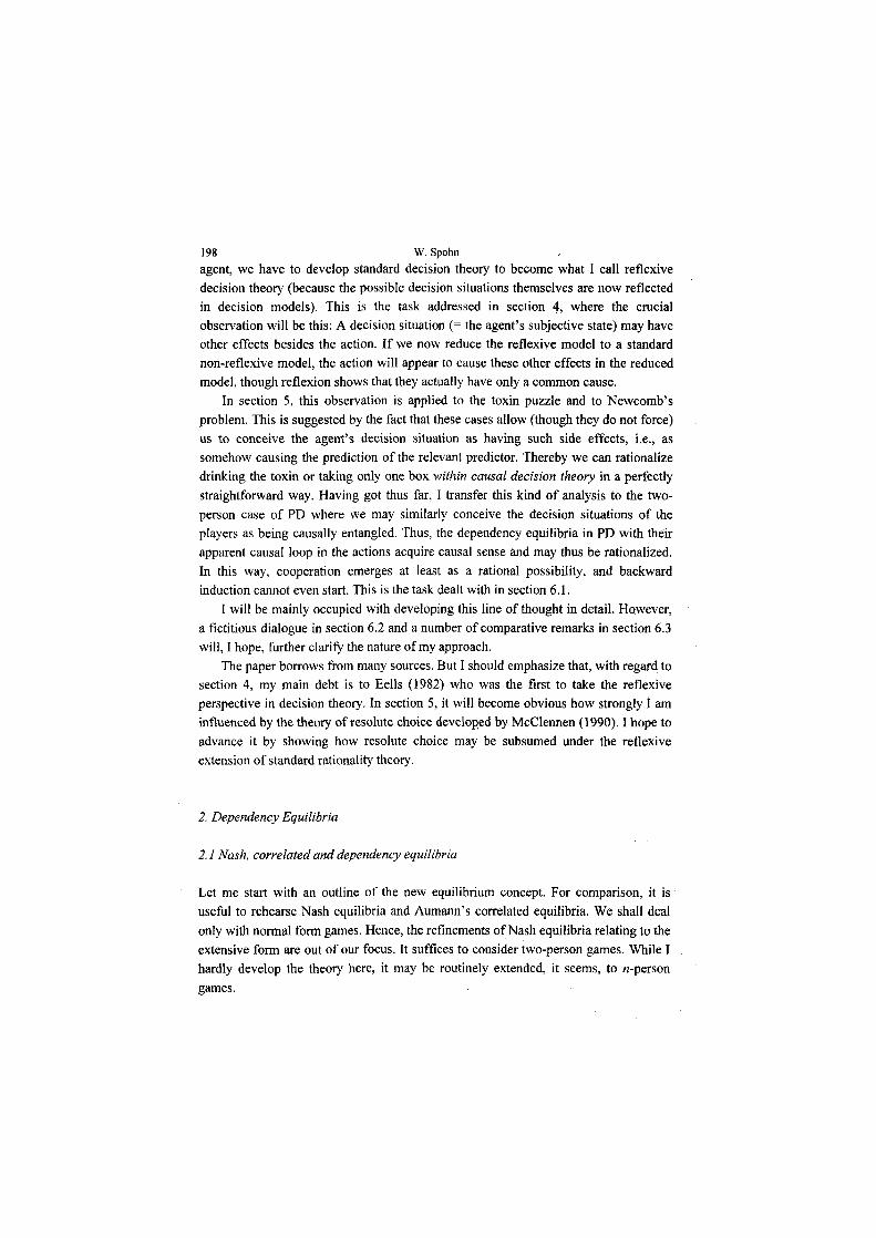
Dependency Equilibria 203By contrast, it is easily verified that the dependency equilibria of this game may bebiased toward the diagonal or toward the counter-diagonal:

P | bi ha\ x y-t-x where 0 <~n <yi.03 y^-x x

It is instructive to represent the players' expected utilities in the various equilibria by ajoint diagram:

£v

1 \.

0,5 \'————l———-)———>

• : Nash, corr.- :depend.

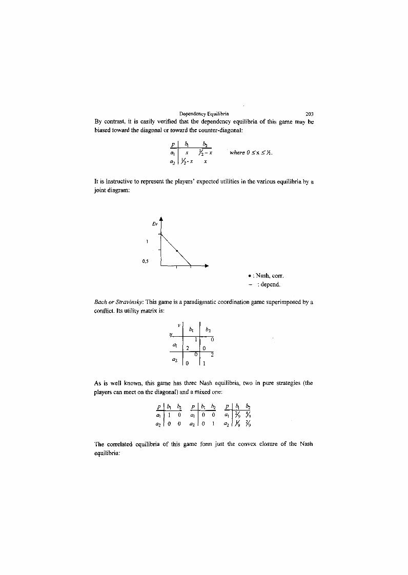
Bach or Stravinsky: This game is a paradigmatic coordination game superimposed by aconflict. Its utility matrix is:

v &1 &2U___ _____ ____

1 0a\ 2 0

0 202 0 1

As is well known, this game has three Nash equilibria, two in pure strategies (theplayers can meet on the diagonal) and a mixed one:

P | b\ bj p \ ft, hi p I fe| ^ai 1 0 fli 0 0 Oi % %02 0 0 02 0 l a-i y^ %

The correlated equilibria of this game form just the convex closure of the Nashequilibria:

204 . W. SpohnP | ^l______ha\ x < 2x, 2y

^ ^ /2, ^

The dependency equilibria are again of three kinds:

p b\ &2 P b\ bi0) 1 0 ai 0 0a; 0 0 02 0 l

provided the zero rows and columns are approximated in an appropriate way, and

P | i b!0) x ^ - x , where 0 <x ^ .fl2 y^-x x

The players' expected utilities in these equilibria come to this:

Ev"

».2

i - J/--"\* * : Nash

2/3 ./ — : corr.», -:depend.

2/3 \ 2 Eu

Quite similar observations can be made about pure coordination games withoutconflict like meeting at one of two places.

Hawk and Dove: This game represents another very frequent type of social situation. Itwill show even more incongruity among the equilibrium concepts. So far, one mayhave thought that the correlated equilibria are the convex closure of the Nashequilibria. But this is not true. I shall consider the utility matrix preferred by Aumannbecause it illustrates that there are correlated equilibria which Pareto-dominatemixtures of Nash equilibria; hence, both players may improve by turning to correlatedequilibria. However, they may improve even more by looking at dependencyequilibria. Here is the utility matrix:

Dependency Equilibria 205v

. ^ ^————^——7

a1 6 2————2"——ö

02 7 0

There are again three Nash equilibria with the following expected utilities:

P | i ^2 P | fe! ^2 J? l b\ biai 0 l ai 0 0 ai % %

03 0 0 a^ l 0 a; % ^The correlated equilibria reach out further on the diagonal. They are given by

I.I.I - £v

1 ~ •

14/3 -

1———————r->

P \b\ hia^ x y , -where x+y+z+w = l and 0 < %, 2w <y, za^ z w

and they yield the following expected utilities:

7.7.2 ^

" ,^\21/4 I——1>^ ,——^

18/5

206 W. SpohnAgain, we have three kinds of dependency equilibria:

p b\ b^ p A] b^a ,~ - 0r ^~ 0 0o; 0 0 a; l 0

provided the zero rows and columns are approximated in an appropriate way, and

P | i ^2Of x y , where y =a;, y \-x-1y

• (2 -15x + ~lS6xT9?).

This makes evident that we slip into quadratic equations. The corresponding expectedutilities reach out still further on the diagonal:

1.1.4 - Ev~ •

76 /

/- *

2

Clearly, 6 > 21/4 > 14/3, the maximal values reached on the diagonals of the threediagrams.

Prisoners' Dilemma: This is my final and perhaps most important example. Its utilitymatrix is:

. 1 \| \————T——3

01 2 0——G-—r

02 3 l

There is only one Nash equilibrium:

Dependency Equilibria 207P \ &i l>ia, 0 0

a; 0 l

Indeed, defection (= a; or, respectively, bt) strictly dominates cooperation (= a\ or b\};hence, there can be no other Nash equilibrium. For the same reason, this is also theonly correlated equilibrium.The dependency equilibria, by contrast, have a much richer structure. They come intwo kinds:

P | bt______b___-a, \x{\. +x) ^ x(l - x) , where 0 <x<l, andfl2 ^x(l-x) ^(\-x)(2.x)

P | h________fr,fli |(l-x)(l+x) ^(l-x)(l-3x) ,where-\ -<x-<^.02 -^(l+x)(l+3x) ^(l-x)(\+x)

The expected utilities in all these equilibria look very simple:

Ev^

•: X1 •; Nash, corr.

'———i———i——>

- : depend.

It is of particular interest here that joint cooperation is among the dependencyequilibria; indeed it weakly Pareto-dominates all other such equilibria. Of course, it isa well-worn and very simple observation that such dependence between the playersmay make them cooperate. But now we have found an equilibrium concept thatunderpins this observation. Moreover, we have seen that correlated equilibria do notprovide the right kind of dependence for this purpose, they succumb to defection.Evidently, all this is strong motivation to try to make good sense of dependencyequilibria. This is the task I shall pursue in the rest of the paper.

208 W.Spohn2.3 Some observations

For the moment, I shall not further discuss or assess these examples beyond theillustrations given. However, the examples suggest some simple generalizations, all ofwhich can be extended, it seems, to thew-person case.

Observation 1: Each Nash equilibrium of a two-person game is a correlatedequilibrium.Proof. Just look at the definitions.

Observation 1: The set of correlated equilibria of a two-person game is convex.Again, the proof is evident from the definition. Of course, we find both

observations already in Aumann (1974, sect. 4). They entail that the convex closure ofthe Nash equilibria of a game is a subset of the set of correlated equilibria.

The next observations are closer to our concerns:

Observation 3: Each Nash equilibrium of a two-person game is a dependencyequilibrium.Proof. Again, just look at the definitions.

Observation 4: Generally, dependency equilibria are not included among the correlatedequilibria, and vice versa.Proof. Just look at the examples above.

In BoS we saw that there are also very bad dependency equilibria, and in PD weluckily found one dependency equilibrium weakly Pareto-dominating all the others.This suggests the following question: Which dependency equilibria are Pareto-optimalwithin the set of dependency equilibria? Clearly, these are the most interesting orattractive ones. Here is a partial answer:

Observation 5: Let q = s ® t be a Nash equilibrium and suppose that the pure strategycombination (a„bic) is at least as good as this equilibrium, i.e., that u^ > ^ t, iiß

j.iand v^ > '^s. ti v.i. Then this combination, or p with pit = 1, is a dependency equili-

j,ibrium.

Proof. Define p1' = £^ •p +J •q, and assume that// is strictly positive. Obviously lim/—»00

p = p. Moreover, lim ^p/'ji •My = u , and for ally ^ / and all r .p/'j, •M,/ = '/ •",;•r->co , ; ,

Dependency Equilibria 209But now we have u^ >. Sjtiiiji ä tiUß: the first inequality holds by assumption and

J.I I

the second because (s, t) is a Nash equilibrium. The same considerations apply to theother player..Hence, given our assumption, with put = 1 is a dependency equilibrium.

If^/ should not be strictly positive, modify q such that those a, withy ^ ;' and s(aj}= 0 receive some positive probability by q and such that q(bi \ aj) = ti, andcorrespondingly for those &/ with / ^ k and t(bi) = 0. Then the modified p is strictlypositive, and the same proof goes through.

In PD, Hawk and Dove, and BoS this observation fully satisfies the quest for thePareto-optima among the dependency equilibria. But it does not generally do so. InMatching Pennies no pure strategy combination is Pareto-better than the Nashequilibrium; yet mixtures of them in which equivalent strategy combinations haveequal weight are dependency equilibria.

This accentuates how preliminary my formal investigation of dependencyequilibria is. However, it is not yet clear whether dependency equilibria are at all worththe efforts. If the answer we shall find is convincing, this may be sufficient motivationto deepen the formal investigation.

3. Causal Graphs, Bayesian Nets, Reductions, and Truncations

I have mentioned that dependency equilibria seem to be a causal mystery. For the sakeof clarity, it is helpful to look at some basics of the probabilistic theory of causationwhich has become sort of a standard (if there is any in this contended area). This pieceof causal theory will clearly confirm some fundamental assumptions of decision andgame theory that are causally motivated, but probabilistically expressed. Thus, it willat first deepen the mystery about dependency equilibria. At the same time, however,we shall be able to see more clearly how to gain a different view.

3.1 Causal graphs and Bayesian nets

The standard theory I am alluding to is the theory of causal graphs and Bayesian nets.'2

It deals only with causal dependence and independence between variables. In order to

"This theory has been discussed more or less explicitly in the statistical path analysis literature sinceWright (1934) and in the linear modeling literature since Haaveimo (1943) and the papers collected inSimon (1957). The structure and the crucial role of the general properties of conditional probabilisticindependence seem to have been recognized not before Spohn (1976) and Dawid (1979). Pearl andhis collaborators rediscovered these properties and added the graph theoretic methods as summarizedin Pearl (1988). Since then an impressive theoretical edifice has emerged, best exemplified by Spirteset al. (1993), Shafer (1996) and Pearl (2000).

210 W. Spohndo so, it must consider specific variables and not generic ones. Generic variables, say,of a sociological kind, would be annual income or social status. But it is usually veryhard to say anything substantial about causal relations between generic variables.Specific variables of a sociological kind would be, e.g., my income in 2001 or mysocial status in 2002, insofar they are understood as ranges of possible values thevariables may take, and not as facts consisting in the values the variables actually take.Hence, the realization of specific variables is always located at a specific time andusually also at a specific place or in a specific object or person.

The basic ingredient of the causal standard theory is thus a non-empty set U ofvariables which we assume to be finite; U is also called a frame. We may representeach variable by the (finite) set of the possible values it may take (this presupposes thatthe variables are mutually disjoint sets). For V U, each member of the Cartesian

product XFofall the variables or sets in V is a possible course of events within V, apossible way how all the variables in V may realize.

Due to their specificity, the variables in U have a temporal order <. A < B says thatA precedes B." I assume < to be a linear (and not a weak) order, thus avoidingquestions about simultaneous causation. Moreover, due to their specificity thevariables in U also display causal structure; their causal order is a partial orderagreeing with the temporal order. That is, if A => B expresses that A influences B or Bcausally depends on A, then => is a transitive and asymmetric relation in U, and A => Bentails A < B.

Since U is finite, we can break up each causal dependence into a finite chain ofdirect causal dependencies. This simplifies our description. If A —> B expresses that Adirectly influences B, or B directly causally depends on A, then —> is an acyclic relationin U agreeing with the temporal order, and => is the transitive closure of-». Of course,directness and indirectness is relative here to the frame U; a direct causal dependencein Umay well become indirect or, as we shall see, even spurious in refinements of U.

Graphs are relations visualized. Thus, we may say as well that (U, —>) is a directedacyclic graph agreeing with the temporal order1'1 or, as we define it, a causal graph. Letme introduce some terminology we shall need:

Pa(B) = the set of parents of B = {A \ A -> B},Pr(B) = the set of variables preceding B = {A \ A < B} , andNd(B) = the set of non-descendants o!B= { A \ A B and not B => A}.

"This is not the A and B from sect. 2. From now on A, B, C, etc. are used to denote any singlevariables whatsoever. Of course, A and B from sect. 2 are also variables.'"The temporal order is often left implicit or neglected, presumably because the statistical literature ismore interested in generic variables. However, as long as one is not engaged in the project of a causaltheory of time, one must presuppose temporal order when talking about causation.

Dependency Equilibria 211

A small example may be instructive. It is Pearl's favorite. The indices indicate thetemporal order:

(Af) (slippery pavement: yes/no)

t(A^\ (wet pavement: yes/no)

^ ^(rain: yes/no) (A^\ (K\ (sprinkler: off/on)

^r^i/( 1 1 (season: spr./sum./aut./win.)

This is a very simple causal graph showing how the season influences the wetness ofthe pavement via two different channels, and the wetness in turn directly influences theslipperiness.

So far, we have just structure. However, the causal structure must somehow relateto how the variables realize, and since we shall consider realization probabilities here,this means that the causal structure must somehow relate to these probabilities. Ishould emphasize that these probabilities may be objective ones (whatever this meansprecisely), in which case they relate to the objective causal situation, or they may besome person's subjective probabilities, in which case they reflect the causal beliefs ofthat person." The latter perspective will be the relevant one for us.

But what exactly is the relation between causation and probability? Spirtes et al.(1993) state two crucial conditions, the causal Markov condition and the minimalitycondition. In order to explain them, we need the all-important notion of conditionalindependence:

Let p be a probability measure for U (i.e., p(v) S 0 for each v e XU and^ p(v) = 1). Then, for any mutually disjoint sets of variables X, Y, Z c U Xis said to

vextlbe conditionally independent of Y given Z w.r.t. p - in symbols: XL Y l Z - iff for all

x 6 XX, y ^ X Y and z 6 XZ p(x\y^) = p(x\z), i.e., if, given any completeinformation about Z, no information about Y teaches us anything about X.

Conditional probabilistic dependence is closely tied up with causal dependenceaccording to a causal graph (U, —>). The causal Markov condition says that, for all

"This assertion sounds nice, and I do not think it is really wrong, but it deserves a most carefulexplanation. In fact, it is the most profound philosophical problem with causation what to say hereprecisely.

212 W. Spohn

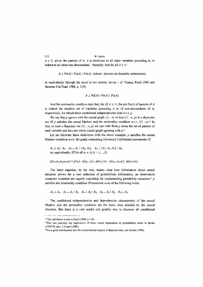
A e U, given the parents of A, A is irrelevant to all other variables preceding it, orindeed to all other non-descendants - formally: that for all A e U

A 1 Pr[A) \ Pa(A) I Pa(A) (where \ denotes set theoretic subtraction),

or equivalently (though the proof is not entirely trivial - cf. Verma, Pearl 1990 andtheorem 9 in Pearl 1988, p. 119):

AlNd(A)\Pa(A)/Pa(A).

And the minimality condition says that, for all A e U, the set Pa[A) of parents of Ais indeed the smallest set of variables preceding A or of non-descendants of A,respectively, for which these conditional independencies hold w.r.t. p.

We say that/? agrees -with the causal graph (U, —>) or that {U, —>, p) is a Bayesiannet iff p satisfies the causal Markov and the minimality condition w.r.t. (U, —>)." Infact, in such a Bayesian net {U, —>,p) we can infer fsomp alone the set of parents ofeach variable and thus the whole causal graph agreeing with^.'7

Let me illustrate these definitions with the above example: p satisfies the causalMarkov condition w.r.t. the graph concerning (obviously Califomian) pavements iff

A^ IA^ /A^ , A4±Ai/{Az,A^, A^l.[A\,Ai,A^IA^,or, equivalently, iff for all a, 6 A, (i = 1,...,5)

p(a\, 02,03,04,05) =p(a\) • P(ai I 01) • p(a^ \ a,) • p(cn \ 02,03) • p(a-, ] 04).

The latter equation, by the way, makes clear how information about causalstructure allows for a vast reduction of probabilistic information, an observationcomputer scientists are eagerly exploiting for implementing probability measures."/?satisfies the minimality condition iff moreover none of the following holds:

A-tIA^, A-,,\-A\IA-i, A^lA-i /A^, A^lA-s/Az, A^IA^.

The conditional independencies and dependencies characteristic of the causalMarkov and the minimality condition are the basic ones entailed by the causalstructure. But there is a very useful and graphic way to discover all conditional

" This definition is due to Pearl (1988, p. 119)."This was precisely my explication of direct causal dependence in probabilistic terms in Spohn(1976/78, sect. 3.3) and (1980)."For a good introduction into the computational aspects of Bayesian nets, see Jensen (1996).

Dependency Equilibria 213dependencies and independencies implied by the basic ones. This is delivered by theso-called criterion of d-separation." Let us say that a path in the graph (U, ->)2° isblocked or d-separated by a set Z c I/of nodes (or variables) iff

(a) the path contains some chain A -> B -> C or fork A <- B -> C such that the middlenode B is in Z, or

(b) the path contains some collider A—> B <— C such that neither B nor any descendantof B is in Z.

We continue to define for any mutually disjoint X, Y, Z c U that Z d-separates Xand FiffZ blocks every path from a node in X to a node in Y.

The notion may look complicated at first, but one becomes quickly acquaintedwith it. In our sample graph, for instance, A-i. and Ai, are d-separated only by {A\}, butneither by 0 nor by any set containing Ai, or A}.

The importance of d-separation is revealed by the following theorem: For all X, Y,Z c U, if X and Y are d-separated by Z, then X 1 Y I Z according to all measures pagreeing with (U, —>); and conversely, \ fX and Y are not d-separated by Z, then not X1 Y I Z according to almost all p agreeing with (U, ->)." This shows that d-separationis indeed a reliable guide for discovering conditional independencies entailed by thecausal structure, and in fact all of them for almost all measures. We shall make use ofthis fact later on.

Spirtes et al. (1993) define a causal graph (U, ->) and a probability measurer forU to be faithful to one another iff indeed for all mutually disjoint A", Y, Zc UX1 Y I Zw.r.t. p if and only if X and Y are d-separated by Z.2' Thus, the second part of thetheorem just stated says that almost all p agreeing with (U, —>) are faithful to (U, —>).But sometimes it is useful to exclude the exceptional cases by outright assumingfaithfulness.

3.2 Reductions of causal graphs and Bayesian nets

An important issue in the theory of causation is how causal graphs and Bayesian netschange with changing frames. If the frame is extended there is no determinate answer

"Invented by Thomas Verma; see Verma, Pearl (1990), and also Pearl (1988, p. 117)."A path is just any connection between two nodes disregarding the directions of the arrows, i.e., anysequence <A1,..., An) of nodes such that for each i = l,...,n-l either Ai -> Ai+1 orAi <- Ai+1."Cf. Pearl (2000, p. 18). The proof is involved; see Spirtes et al. (1993, theorems 3.2 and 3.3)."Almost all" is here understood relative to the uniform distribution over the compact space of allprobability measures for U."This is not quite faithful to Spirtes et al. (1993). Their definition of faithfulness on p.56 is a differentone, and in their theorem 3.3 they prove it to be equivalent with the definition given here.

214 W.Spohnbecause probabilities can be arbitrarily extended to the richer frame. But if we startwith a Bayesian net on a large frame and reduce it, then the Bayesian net on thereduced frame must have a definite shape. The question is which one.

Let us simplify matters by focussing on reductions by a single variable only.Larger reductions can then be generated by iterating such minimal reductions. So, howdoes a causal graph change when a node, C, is deleted from the frame U7 The answer,which is not entirely obvious, is prepared by the following definition:The causal graph (U*, ->•*) is called the reduction of the causal graph (U, —>) by thenode C iff:

l. U* = U\ {C},1. for all A, B e U* A ->* B iff either A -> B, or not A -> B and one of the following

three conditions holds:(i) A -> C -> B (let us call this the IC-case), or(ii) A<BmdA<-C->B (let us call this the CC-case), or(m)A < B and there is a variable D < B such that A —> D <- C -> B (let us call thisthe N-case).

Thus, the reduced graph contains all the arrows of the unreduced graph notinvolving the deleted variable C. And it contains an arrow A ->* B where theunreduced graph contains none exactly when B is rendered indirectly causallydependent on A by the deleted C (the IC-case), or when the deleted C is a commoncause of A and B (the CC-case), or when A is the neighbor of such a CC-caseinvolving B (the N-case).

The N-case may look a bit complicated. Let us make it more graphic (as anothermnemonic aid for its label):

@ ., ®® / @ ^ - 7

/1 ^\ / reduces to ^ ^^

® © @

The N-case is always accompanied by a CC-case. Note the importance of thetemporal relation D<B.lfB<D,we only have a CC-case involving B and D, where

® © /^ \ ® ^ ^^ ®

/ \ /' reduces to /

@ © ®


The justification for this definition is provided by the following theorem: Let (U,—>, p) be a Bayesian net, let (U*, ->*) be the reduction of {U, —>) by C, and let p* bethe marginalization or restriction ofp to U* = U\ {C}. Then the causal graph agreeingwithp* is a (proper or improper) subgraph of(U*, ->*), and ifp is faithful to (U, —>),then it is (U*, —>*) itself which agrees withp*.

Proof: Suppose that B directly causally depends on A w.T.t.p*, i.e., that not A 1 B lX, where X= Pr(B) \ {A, C}. We need not specify here relative to which probabilitymeasure the conditional (in)dependence statements are to be taken, because p and;?*completely agree on them within U*. According to the above theorem about d-separation not A l B l X entails that A and B are not d-separated by X in (U, ->). Thismay be so because A —>• B or because the 1C-, the CC-, or the N-case obtains, but in noother case; in all other cases each path between A and B must be blocked by X, as iseasily checked. Hence, not A -L B I X entails A —>* B. This proves the first part of thetheorem.

Now, suppose that B does not directly causally depend on A w.r.t. p*, i.e., that A 1B I X, and suppose thatp is faithful to (U, —>). Hence, A and B must be d-separated byX in (U, —»). Therefore, as we have just seen, neither A —> B nor one of the 1C-, CC-,or N-case can obtain. That is, A —> B does not hold. This proves the second assertionof the theorem.

In the case that p is not faithful to (U, —>), the theorem cannot be strengthened,because in that case there may hold a lot of conditional independencies not foreseen bythe criterion of d-separation. Hence, d-separation may tell us A —>* B, even though A1 B I X, which excludes a direct causal dependence of 5 on A w.r.t. p*.

However, if p is faithful to (U, —>), this situation cannot arise, and we have acomplete answer about the behavior of reductions." Indeed, it is more illuminating toreverse the perspective again and to read the theorem not as one about reductions, butas one about extensions. Our picture of the world is always limited, we always movewithin a small frame U*. So, whenever we construct a causal graph (U*, —>•*) agreeingto our probabilities p*, we should consider this graph as the reduction of a yetunknown, more embracive graph (U, ->). And the theorem then tells us (i) that -wherethere is no direct causal dependence according to the small graph, there is none in theextended graph, and (ii) that what appears to be a direct causal dependence in thesmall graph may be either confirmed as such in the extended graph, or it may turn outto be spurious and to resolve into one of the 1C-, CC-, or N-case. This observation willacquire crucial importance in sections 4 and 5. To be precise, the observation is

"One should note, though, that even if p is faithful to <U, -»>, p* need not be faithful to <U*, ->*).Indeed, p* cannot be faithful if the N-case applies, since in that case we have A 1 B, though A and Bare not d-separated by 0 in (U*, -»*).

216 W.Spohnguaranteed only if the extended probabilities p are faithful to the extended graph (U,—>). But since almost all probability measures agreeing with (U, —>) are faithful to it,we may reasonably hope to end up with such a p.

So much for the standard theory of probabilistic causation. Calling it standard isperhaps justified in view of the impressive list of its predecessors and defenders. It isalso more or less explicit in a great deal of applied work and in particular in large partsof decision and game theory. But it is still contested, most critically perhaps byCartwright (1989, 1999), who splits up the causal Markov condition into two parts, aproper Markov condition relating only to the past of the parents of the relevant node,and a screening-off condition (as in Reichenbach's principle of the common cause)relating to the other non-descendants. Cartwright accepts the proper Markov condition,but vigorously rejects the screening-off condition. This is tantamount to the assertionof interactive forks, as introduced and defended by Salmon (1980, 1984).

But even if the theory is not contested, the underlying conceptions may be quitedifferent. In Spohn (2001) I have elaborated, for instance, on the differences betweenmy picture and that of Spirtes et al. (1993). It is important to know of thesedivergences; in philosophy no opinion is really standard in the end. In the following,though, I shall neglect these debates and proceed with the theory to which I refer as thestandard one.

3.3 Actions, truncations, and basic decision models

So far, actions and agents have not entered the picture. A Bayesian net describes eithersome small part of the world or some person's partial view of the world. But thisperson might be a detached observer having only beliefs and no interests whatsoeverabout that part. This, however, is not the agent's view as it is modeled in decisiontheory. In order to accommodate it, we have to enrich our picture by adding twoingredients.

The first ingredient consists in desires or interests that are represented by a utilityfunction. Each course of events is more or less valued, and accordingly a utility

function u is a function from X U into R.So far, we still might have a mere observer, though an interested one. But an agent

wants to take influence, to shape the world according to his interests. Hence, we mustassume that some variables are action variables that are under direct control of theagent and take the value set by him. Thus, the second ingredient is a partitioning of theframe U into a set H of action variables and a set W of occurrence variables, as I callthem for want of a better name.


Are we done now? No. The next important step is to see that not any structure {U,—>, H, p, u) (where W = U\ H) will do as a decision model; we must impose somerestrictions.

A minor point to be observed here is that H does not contain all the variables in Uwhich represent actions of the agent. Rather, H contains only the action variables stillopen from the agent's point of view. That is, the decision model is to capture theagent's decision situation at a given time t. Thus, H contains only the action variableslater than t, whereas the earlier variables representing acts of the agent are alreadypast, no longer the object of choice, and thus part of W.

Given this understanding ofH, the basic restriction is that the decision model mustnot impute to the agent any cognitive or doxastic assessment of his own actions, i.e., ofthe variables in H. The agent does not have beliefs or probabilities about H. In the firstplace, he has an intention about H, formed rationally according to his beliefs anddesires or probabilities and utilities, and then he may as well have a derivative beliefabout H, namely, that he will conform to his intention about H. But this derivativebelief does not play any role whatsoever in forming the intention. I have stated this"no probabilities for acts" principle in Spohn (1977, sect. 2) since it seemed to me tobe more or less explicit in all of the decision theoretic literature (cf, e.g., Fishbum1964, pp. 36ff.) except Jeffrey's evidential decision theory (1965); the principle wasalso meant as a criticism of Jeffrey's theory. The arguments I have adduced in its favorhave been critically examined by Rabinowicz (2002). My present attitude toward theprinciple will become clear in the next section.

It finds preliminary support, though, in the fact that it entails another widelyobserved principle, namely, that the action variables in H are exogenous in the graph{U, ->), i.e., uncaused or parentless. Why does this "acts are exogenous" principle, asI call it here, follow? If the decision model is not to contain probabilities for actions, itmust not assume a probability measurer for the whole of U. Only probabilities for theoccurrence variables in W can be retained, but they may, and should, be conditional on

the various possible courses of action h e X//: the actions may, of course, matter to

what occurs in W. Hence, we must replace the measure p for U by a family (ph)he'xn ofprobability measures for W. Relative to such a family, Bayesian net theory still makesperfect sense; such a family may also satisfy the causal Markov and the minimalitycondition and may agree with, and be faithful to, a given causal graph.2" However, itcan do so only when action variables are parentless. For a variable to have parents inagreement with the probabilities, conditional probabilities for it must be explained, but

"My definitions and theorems concerning conditional independence in Spohn (1978, sect. 3.2) dealtwith the general case relating to such a family of probability measures. The graph theoretic materialmay be supplemented in a straightforward way.

218 W.Spohnthis is just what the above family of measures must not do concerning action variables.Therefore, these variables cannot have parents.

Pearl (2000, ch. 3) thinks along very similar lines when he describes what he callsthe truncation of a Bayesian net: He starts from a Bayesian net (U, —>,p). U contains asubset H of action variables, p is a measure for the whole of U and thus representsrather an external observer's point of view. Therefore, the action variables in H haveso far no special role and may have any place in the causal graph (U, ->). Now Pearlimagines that the observer turns into an agent by becoming empowered to set thevalues of the variables in H according to his will so that the variables in H do notevolve naturally, as it were, but are determined through the intervention of the agent.Then Pearl asks which probabilities should guide this intervention. Not the whole of p.Rather, the intervention cuts off all the causal dependencies the variables in H haveaccording to (U, —>) and puts itself into place. Hence, the agent should rather considerthe truncated causal graph (U, —>*) which is defined by deleting all arrows leading toaction variables, i.e., A —>* B iff A —> B and B t H. Thereby the action variables turnexogenous, in accordance with our principle above.

The next task is to find the probabilities that agree with the truncated graph. We

must not simply put ph(w) = p(w \ h) (h e Y-H, w e X W); this would reestablish thedeleted dependencies. Rather, we have to observe the factorization of the whole of pprovided by the causal graph (U, -») (which I have already exemplified above with theCalifornian pavements):

If v e X U is a course of events in U u and if for each A e U a is the value A takesaccording to v and pa(a) the values the variables in Pa(A) take according to v, thenP^ = I! P(a\pa(a)).

AeU

Then we have to use the truncated factorization2' that deletes all factors concerningthe variables in H from the full factorization;

If h e XH and w e X W and if for each A e W a is the value A takes according tow and pa(a) the values the variables in Pa(A) take according to h and w, thenPh(w) = PI P(a\Pa(a))•

AelV

For the family (ph) thus defined, we say that (U, —>*, (pi,)) is the truncation of(U,—>, p) with respect to H, and we can easily prove that (ph) agrees with (U, —>*) if pagrees with (U, —>); this is built in into the truncated factorization. Thus, as Pearl and Iagree, it is this family (ph) that yields the probabilities to be used by the agent. Hence,

"1 use „v" since„u" is already reserved for the utility function."Cf. Pearl (2000, p. 72).

Dependency Equilibria 219Pearl also subscribes to the two principles above." The notion of truncation willreceive a crucial role in sections 4 and 5.

We may resume this discussion by defining a basic decision model. This is astructure (U, —>, H, (ph), u), where (U, -») is a causal graph, H is a set of exogenousvariables, (ph) Is a family of probability measures for ^agreeing with (U, —>), and u a

utility function from X U into J?.What is the associated decision rule? Maximize conditional expected utility, i.e.,

choose a course of action h e XH for which ^ u(k,w)-p^(w) is maximized.weXIV

However, this decision rule is naive insofar as it neglects the fact that the agent neednot decide for a whole course of action; rather, he needs to choose only from the(temporarily) first action variable and may wait to decide about the later ones. Thus thenaive decision rule has not taken into account strategic thinking. We shall have severalreasons for undoing this neglect below.

So far, I have not really argued for the two principles and thus for the given basicform of decision models. I have only claimed that it is more or less what we find inmost of the decision theoretic literature. I find it very natural to read Savage (1954)and Fishbum (1964) in this way, and I have referred to the more recent literature aboutcausal graphs such as Spirtes et al. (1993) and Pearl (2000). This is not an argument,but it carries authority. We shall continue the topic in the next section.

Let me point out an important consequence, though. In a basic decision model allnon-descendants of an action variable are probabilistically independent of it. This isentailed by the exogeneity of action variables, as is easily verified with the help of d-separation. In other words: what is causally independent from actions is alsoprobabilistically independent from them.

This observation provides an immediate solution of Newcomb's problem.2'According to Noziek (1969), the initial paper on the problem, Newcomb's problem isconstituted by the fact that there may be events (such as the prediction of themysterious predictor) which are causally independent from my actions, butnevertheless probabilistically relevant. According to the observation just made, thisalleged fact is spurious; there are no such events, and hence there is no Newcomb'sproblem, as I have explained in Spohn (1978, sect. 5.1). Of course, there is more to sayabout Newcomb's problem, and I shall say more below. But I believe that thereby the

"In this paragraph I have slightly assimilated Pearl's conception to mine, though in a responsibleway, I believe. In principle, the truncation procedure is already described in Spohn (1978, pp. 187ff.),though without graph-theoretic means. It should also be noted that Spirtes et al. (1993, pp. 7Sff.)make essential use of the transition from unmanipulated to manipulated graphs, as they call it. Thistransition closely corresponds to Pearl's truncation."For a presentation of Newcomb's problem, see sect. 5.

220 W. Spohnstubborn intuition of two-boxers, which I have espoused for more than 20 years, iswell explained: if Newcomb's problem is modeled by a basic decision model, two-boxing is the only rational action.

The observation also explains a constitutive feature of non-cooperative gametheory, namely, that the actions of the players are causally independent; they do notcommunicate or interact in any way. And the players have to be aware of this causalindependence. Hence, if this observation is correct, the players' actions areprobabilistically independent as well (also from their own point of view). This is whathas been assumed all along in non-cooperative game theory, and this is why we seemto be forced to adopt something like Nash equilibria, which are the only equilibriaconforming to this probabilistic independence.

All this shows that basic decision models as defined above are deeply entrenchedin decision and game theoretic thinking. The last point, in particular, underscores thesuspicion, raised in section 2, that dependency equilibria do not make causal sense.Thus, our search for causal sense can only take one direction: we have to scrutinize theassumptions underlying basic decision models. This is our next task.

4. Reflexive Decision Theory

How can one doubt the "no probabilities for acts" and the "acts are exogenous"principle? I see essentially two ways. On the one hand, the agent himself may make hisactions dependent on the behavior of other variables and thus turn the action variablesinto endogenous ones; this is what is called strategic behavior. By deciding for acertain strategy the agent obviously accepts certain probabilities for the actionscovered by the strategy, in contradiction to the two principles. On the other hand, it ishard to see why the agent should not be able to reflect on the causes of his ownactions, just as he does concerning the actions of others. This reflexion should clearlyenable him to have (probabilistic) predictions about his future actions, again incontradiction to the principles. We shall see that both approaches come to the samething; but let us dwell upon them separately and more carefully.

4. l Dependency schemes and strategies

Let us take up strategies first. Concerning basic decision models, I have alreadymentioned that it would be a naive decision rule simply to choose a course of actionwith maximal expected utility. Usually it is better to wait and see what happens and actaccordingly. How can this be accounted for in our graph theoretic framework?

The most general way is this: According to a given basic decision model (U, —>,H, (pf,), u) all action variables in H are exogenous. What the agent does in thinking

Dependency Equilibria 221about strategies is to enrich the causal graph (U, —>) by some edges each of whichends at some action variable and starts at some preceding occurrence variable; thismeans to reverse the truncation described in the previous section. Of course, the agentdoes not only create such dependencies, he considers to create them in a specific wayexpressed by specific probabilities. This is captured in the following definition: Adependency scheme q for a given basic decision model is a function which specifiesfor each action variable A e H a probability distribution for A conditional on eachrealization ofPr(A), i.e., of all the variables preceding A.

On the basis of the probability family (ph) each dependency scheme q determines a

probability measure pq for the whole of U defined as follows: for w e XW and

h e XH py(h,w) = ph(w) • q(h w) - where q(h \ w) denotes the probability that theaction sequence h realizes according to q given w. That is: if, for A e H, a denotes thevalue A takes according to h andpr(a) the values the variables in Pr(A) take accordingto h and w, then q(h w) = Y[ q(a\pr(a)). These are just the factors we need in order

AeH

to fill up a truncated factorization to yield a complete one.This, in turn, enables us to define the expected utility of each dependency scheme

q: Eu(q)= ^ ^ u(h,w)-pg(h,w). This suggests a more general and reasonableheXH weXW

decision rule: If your situation is represented by the given model, choose a dependencyscheme with maximal expected utility! Is this rule a good one?

No, the problem is that not every dependency scheme represents a feasiblestrategy. I have lost my glasses, for instance. What to do? Clearly, the optimaldependency scheme would be to search in my office if I have forgotten them in myoffice, to look into the fridge if I have put them into the fridge, etc. This would clearlybe the fastest way to find my glasses. But it is obviously not feasible; my problem isjust that I do not know where I have put them. Hence, dependency schemesmaximizing expected utility tell only how the agent and his actions would be optimallyembedded into the causal graph according to his subjective view. Whether he is able toembed himself in such a way is another question.

This raises the following question: Which of the dependency schemes are feasiblestrategies that the agent is able to realize by himself? Generally, one can only say thatthe latter form a convex subset of the former. The reason is the frame-relativity ofdependency schemes. One should think at first that there is no need to considerprobabilistic dependency schemes because it is always better to establish gooddeterministic dependencies. However, there is no guarantee that the frame contains thevariables which the agent is able to connect up with in a deterministic way. Perhapsthe agent at best receives incomplete information about the variables included in theframe. In this case only a probabilistic dependency is within his power. Hence, as long

222 W.Spohnas we do not make special assumptions about which variables are in the frame U, nomore can be said about the feasibility of dependency schemes.

So, we should perhaps include in the frame those variables to which the agent canestablish a deterministic dependence. Which are they? The answer seems clear. Theagent can make his action depend only on those variables whose state he learns beforethe time of action. Maybe his behavior is correlated with the state of certain variables,though he does not notice it. But if so, the behavior is not intentional. Thus, for thedependence to be intentional, the agent has to know the states he wants to correlatewith.

Again, no general statement seems available concerning the kind of variables theagent learns about. They must be observable, for sure; but the decline of empiricismhas shown that this characterization is vague and loose. Still, there is a generalstatement: Whatever the external events the agent does, or does not, notice, he knowshis own state before the time of action, he knows the decision situation he is in (i.e.,his subjective view of it), which is generated, among other things, by the externalevents he has noticed.

This seems generally true. Hence, a general procedure for discovering the feasiblestrategies among the dependency schemes would be to extend the causal graph of thegiven basic decision model by a number of decision nodes, as I call them, such thateach action node is preceded by a decision node, and then to define a strategy as adependency scheme which makes each action node depend only on its associateddecision node. Here, a decision node is quite a complex variable consisting of all thedecision situations the agent might be in concerning the associated action node.Obviously a decision node causally depends, in turn, on many other variables; thereby,the action node's direct intentional dependence on the decision node ramifies intovarious indirect dependencies (where "direct" and "indirect" is relative to the extendedcausal graph). Moreover, it is obvious which deterministic shape the action node'sintentional dependence on the decision node should take: the relevant decision rule,say, maximizing conditional expected utility, states which action to perform in whichdecision situation.

It should be clear that we have to elaborate the content of the previous paragraphsin detail. This is what we shall do in section 4.3. But one point should be stated rightaway. What I have explained so far entails that as soon as the agent has decided for acertain strategy or dependency scheme, he can, on the basis of this decision, predictwith which probability he will perform which action supported by his strategy. This isthe first way for apparently rebutting the "no probabilities for acts" principle.

Dependency Equilibria 2234.2 Reflexion

I have announced a second way, at which we should look next before furtherdeveloping the above ideas. This way is even more straightforward: Why should theagent be unable to take doxastic attitudes like predicting, explaining, etc. toward hisown actions, if he can very well do so toward the actions of others? One should indeedthink that he is particularly well endowed in his own case because he has so muchmore data about himself than about anybody else.

Hence, the question is rather: How should the agent predict his own futurebehavior? There seem countless ways. The agent knows his habits ("sure, I'll brush myteeth this evening when I go to bed; that's what I always do!") or the conventions ("ofcourse, I'll drive on the right tomorrow; everybody does!"), he knows his anxieties andthe resulting behavior ("I won't hike through Devil's gorge!"), and so on. All thesepieces of behavior may, or may not, be under the rational control of the agent. If theyare, as is likely in the case of habits and conventions (at least in the examples given),the prediction is incomplete unless it mentions that the particular instantiation of ahabit or convention is confirmed by rational control. This means, in turn, that theprediction of a piece of behavior is really based on the prediction of the (tacit orexplicit) rational deliberation leading to it. If a piece of behavior is not under rationalcontrol, as it may be in the case of anxiety, then, it seems to me, it cannot be the objectof a practical deliberation and does not deserve the status of an action node in adecision model; from the point of view of a practical deliberation, it is just anoccurrence to reckon with, not an action to be intentionally chosen.2'

To conclude, the agent should predict and explain his actions at future actionnodes as intentional and rational actions with the help of decision theory, just as heexplains and predicts the actions of others. Hence, if we want to make explicit thesemeans for predicting and explaining actions within the decision model, we shouldextend it by decision nodes, as we have envisaged them in our discussion of strategies.The agent has (probabilistic) predictions about the decision situations he will face, andaccordingly he has (probabilistic) predictions about the future actions, again just as inthe case of strategies.

It may seem surprising how the active mode of considering which feasible strategyto choose and the passive mode of predicting future actions can come to the samething. But it is not so surprising, after all; the two modes melt into each other in thisspecial case. If I predict my likely future actions from my likely future decisionsituations, this is like forming a conditional intention. And conversely, if I chooseamong feasible strategies that make future actions dependent on future decision

"Psychology and self-observation teaches that this distinction is not clear-cut at all. However, for thesake oftheoprizing we sometimes have to paint black and white.

224 W. Spohnsituations, the chosen dependence is not really subject to my present evaluation andintention. Rather, all the parameters on which the evaluation and intention is based,i.e., the relevant subjective probabilities and utilities, are already specified in the futuredecision situation on which the action depends; the decision is deferred to thatsituation. One description is as good as the other; and so the active mode of decisionand the passive mode of prediction merge.

Thus, it seems that we have a convincing double safe argument against ourprinciples. Did we succeed to refute them? It is not clear whether this conclusionwould help with the task set at the end of section 3. And it would be premature, in anycase. Before jumping to conclusions, we should rather scrutinize how decision modelsthat include decision nodes really look like.

4.3 Reflexive decision models and their truncated reductions

In section 4.1 I have already sketched such reflexive decision models, as I would liketo call them, since they model how the agent reflects on his own attitudes. Thesemodels need to be worked out. The resulting structure, however, will be very complex;we cannot and need not fathom it here in full depth. I shall render precisely only thoseaspects required for my argument; the others will be left sketchy.

Here is my proposal in the form of an extensively annotated partial definition: 8 =(U, —>, H, D, p, u) is a reflexive decision model iff the following conditions (1) - (8)are satisfied:

(\)H, the set of action variables, and D, the set »{decision variables, are disjoint sub-sets of U; as before, W= U\(HuD) is the set of occurrence variables.

This simply introduces the decision variables as new ingredients.

(2) (U, ->) is a causal graph such that each action node has exactly one decision nodeas the only parent, i.e., for each A 6 H there is a A e D with Pa(A) = {A}, and eachdecision node has at least one action node as a child, i.e., for each A e D there is anA effwithAePa(A).

This was the upshot of our preceding discussion. For each action node it is just theparental decision node that provides the intentional or explanatory or predictivedeterminants of which element of the action node is performed. It is thus obvious thatonly decision nodes can be parents of action nodes, and indeed that each action nodecan have only one parental decision node. Thus, (2) is the minimum required.

The question is rather whether (2) should be strengthened. One might require thatno two action nodes have the same parental decision node, or that each action node be

Dependency Equilibria 225immediately preceded in time by its parental decision node.'" One might also wonderhow a decision node can have other children than action nodes. It will be crucial formy argument in the next section to reject all such strengthenings of (2). Therefore, Ishall defer further discussion of this point.

(3) M is a utility function from X((7\ D) into R.

The point of this condition is to exclude the decision nodes from the utilityfunction; in my view, being in, or getting into, this or that decision situation does nothold any utility in itself. I have argued for the point in Spohn (1999, pp. 49ff). Butsince it does not play any role here, I shall not dwell upon it.

(4) p is a probability measure for U.

This reflects the point that there seems to be no restriction on the domain of theagent's probability function under the present perspective. Later conditions, though,will restrict the values p may take.

The next condition is concerns the self-localization of the agent in the reflexivedecision model 8. Such a model is to represent the agent's own practical point of viewresulting in a decision, not that of an external observer. The point is reflected in thefact that H represents his own possible future actions and p and u his own cognitiveand conative attitudes. But at which time? The answer is immediate: the agent is todecide about the first of his action nodes (and possibly later ones as well) and hencefinds himself, as it were, in the first decision node. That is, the time when the agenttakes the attitudes? and u is the time of the first decision node.

At that very time the agent knows in which decision situation he presently findshimself. He may not have foreseen it, and he may have forgotten it later on; but at thetime of decision he knows his subjective view of his situation; and the modelrepresents only this view. This knowledge is captured in the next condition:

(5) If Ac e D is the temporally first decision node, there is a particular 5o e Ao suchthat p(6o) = I."

This is embarrassing, though. So is obviously to represent the present decisionsituation of the agent of which he is aware; on the other hand, the reflexive model 8,

"Since we have assumed the variables to be linearly ordered in time, the second strengthening impliesthe first."This condition of consciousness or self-knowledge has first been stated by Eells (1982, p. 176).

226 W. Spohnwhich we are about to define, does so as well. But 5o is only a part and not the wholeof 8. How can this be?

The first response is that two different decision models, in the present case 5o and5, may well represent the same situation; the representation relation is rarely one-onein model construction. Indeed, if one decision model is a reduction of another, theymay be said to represent the same situation." The second response is that we face ageneral difficulty here. Whenever one models states of reflexion, the object ofreflexion cannot be understood as the whole reflexive state itself." The embarrassmentis thus a common one.

Here is an account of what So is, if not the whole of 6. It is not the basic submodelresulting from the full reflexive model by eliminating all decision nodes; it is only thefirst decision node Ao itself that needs to be eliminated. This elimination results, moreprecisely, in the truncated reduction of 8 by {Ao} defined as follows:

For any decision node A e D, let Ac(&.) denote the set of action children of A(which must not be empty according to condition (2)) and Oc(A) denote the set ofother (occurrence or decision) children of A (which may, but need not be empty).Then, the truncated reduction of 5 by {Ao} is obtained by first reducing 5 by {Ao} notprecisely in the way described in section 3.2, but in a slightly modified way and thentruncating this reduction with respect to^c(Ao). What is the slightly modified way?

Arrows in which Ao is not involved are simply maintained in the reduction asdefined in section 3.2. Likewise, the reduction contains arrows from the parents ofAoto the children of Ao; this is the IC-case. The arrows arriving at action children willthen fall victim to the truncation. (In the following diagrams triangles stand fordecision nodes, squares for action nodes, and circles for occurrence nodes.)

D D D^ A

t—^ reduces to: turns by trun-A '' cation into:

0 0 0(the IC-case)

"I have not explicitly defined the reduction of basic decision models; but our definition of the re-duction of Bayesian nets is easily extended. Such reductions are at the heart of the theory of smallworlds of Savage (1954, sect. 5.5), In Spohn (1978, sects. 2.3 and 3.6) I have elaborated on theirtheoretical importance."This is so at least if we stick to standard ways and do not resort to the model theoretic meansdevised by Barwise (1990), which attempt to accommodate such circular phenomena in astraightforward way.

Dependency Equilibria 227The slight modification occurs in the CC-case. Here, we have to stipulate, for

reasons to be immediately explained, that all arrows between Ac(ô) and Oc(Ao)created by the reduction run from -4c(Ao) to Oc(Ao) irrespective of the temporal order,i.e., even in the case where the arrows thus run backwards in time.

0 ^0 ^0l—l ./ reduces to: l—l ~~ . turns by trun- l—l •'-î

^Ô 0 cation into: O

A

(two CC-cases; the fat arrows show the modification)

This modification entails that the N-case cannot obtain. The modification of theCC-case treats all occurrence children of Ao as if they were later than the actionchildren ofAo, and thus the "N" can take only the form of a simple CC-case:

0 D O^D O^D/ ' •\ ^ reduces to; r turns by trun- r

' \ l • cation into:

0 A 0 0

(no genuine N-case)

Hence, I propose:

(6) 5o = (U\ {Ao}, ->*, H, D \ {Ao}, (pg), u} is the truncated reduction of 8 by {Ao} in

the sense just defined (where g runs through X^c(Ao)).

We have to make clear to ourselves what this amounts to: The causal graph(U\ {Ao}, ->*) of5o is obtained from (U, ->) by deleting, together with Ao, all arrowsending or starting at AO and, provided Oc(Ao) is not empty, by adding arrows from allA e ^c(Ao) and all B e Pa(Ao) to all C e Oc(Ao). The action nodes in Ac (Ao) arethereby turned into exogenous variables, making the other children of Ao, if any,directly causally dependent on all the parents and all the action children ofAo.

This may appear not entirely intelligible. The first mystery may be how a decisionnode may at all have any causal influence that is not mediated by action nodes. But let

228 W.Spohnus grant this point for the moment; it will become clear when we consider specificexamples with non-empty Oc(Ao) in the next section."

The second mystery is the modification of the CC-case which creates arrowsrunning backwards from ^4c(Ao) to earlier members of Oc(Ao). Do we thereby allowfor backward causation? No. Recall our observation in section 3.2 that in a reducedcausal graph an arrow A —> B generally signifies only that B directly causally dependson A or that the 1C-, the CC- or the N-case applies to A and B. Here, it can only be theCC-case which applies to the arrows from Ac(Ao) to Oc(Ao). Note that we had nochoice here but to assume the anomalous backward arrows. If we had added onlyforward arrows in the reduction, i.e., arrows from the earlier members of Oc(Ao) toAc(Ay) and from c(Ao) to the later members ofOc(Ao), then only the latter, but not theformer, would have survived the truncation. But there is no reason whatsoever to treatthe former and the latter arrows in the truncation in a different way; the temporallocation of the members of Oc(Ao) is irrelevant to the causal structure of the situationand should not make any difference. Hence, the information about the common causeof y4c(Ao) and Oc(Ao) has to be completely, and not only partially, retained in thetruncated graph. The only way to do this is by adding in the reduction only arrowsstarting from, and not leading to, ^4c(Ao), as it is shown in the above diagram of theCC-case. This point will be a crucial step of my whole argument because it allows usto interpret critical action dependencies of probabilities as indicating merely a commoncause relation.

Concerning the rest of So, it is clear that 5o contains the same utility function as 8since decision nodes do not carry utilities anyway. The probability family (pp) of 5o,finally, is derived from the measure p of 8 by eliminating the reflexive probability ofcondition (5) and all probabilities entailed by it, in particular the probabilities for theactions in Ac(&,o). The procedures described in section 3 then guarantee that theremaining family (pg) agrees with the reduced and truncated graph."

The upshot of all this is that 5o contains the same decision relevant items as thereflexive model 8 and indeed all of them; the surplus of the reflexive model is only theagent's firm belief that he is in 80 and what follows from this belief. In this way, thecircularity problem that plagued our modeling of reflexive states is solved.

"Let me point out, though, that the presence of this kind of causal influence is a most crucial pointbehind the insightful considerations of Frank (1988). The decision situations in which one findsoneself are accompanied by emotions which show in other ways than merely in the actions optimal inthese situations."There is a familiar problem about conditionalization here. The relation between decision nodes andthe appertaining action nodes will be essentially deterministic. Hence, ifp(50) = 1, then p(g*) = 1 forthe action (course) g* that is optimal in 80 and p(g) = 0 for all other actions g so that pg remainsundefined for them. But the problem is familiar from sect. 1, and it may be corrected with similarmeans. I neglect it here in order to avoid further complications.

Dependency Equilibria 229However, I should emphasize that thereby the "no probabilities for acts" principle

has reentered the picture, if only in relation to the variables in c(Ao); the other actionvariables are taken care of by the later decision nodes. The reason is that 60, whichobserves this principle, contains precisely what is needed for determining or causingthe optimal action. The surplus of the reflexive model has no effect in this respect -though, of course, we can positively assert this only after the decision rule determiningoptimal actions has been introduced."

This is all we need for our present purposes. However, the definition of thereflexive decision model 8 is not yet completed. Let me indicate what is still missing.

For one thing, we require

(7) a condition concerning the shape of all the decision situations 5 in all the decisionnodes A e D.

This condition would not differ so much from our detailed condition (6) on §o. Themost important difference will be that the agent may envisage arbitrary changes ofprobabilities and utilities in all the possible decision situations, whereas theprobabilities and utilities of 5o had, of course, to agree with those of 8. To be sure,theoretical work only becomes substantial by considering various specific forms ofchange. For example, a case that is treated extensively in decision theory is the onewhere the agent deliberates whether first to collect (possibly costly) evidence and thento decide on the basis of probabilities changed accordingly. But many more changesmay be conceived", and conceptually one should allow for all kinds of changes.

Another, final, ingredient is missing, indeed the most difficult and important one:the decision rule that specifies for each possible decision situation what is rationally or >optimally done in it. In our reflexive context, this also determines the agent's beliefsabout the relation between decision and action nodes, since he believes to be and tostay rational (otherwise, it would be wrong from the outset to consider only decisionnodes as parents of action nodes). Hence, the final condition is:

(8) For any decision node A and any situation 8 e A, if g e X^c(A) is irrational in 5according to the relevant decision rule, thenp(g | 6) = 0.

This condition is stated only negatively. In case there are several optimal actions in6 the general model should not ordain specific probabilities for those actions.

"This has been one of my two arguments for this principle in Spohn (1977, sect. 2), the one whichRabinowicz (2001) considers to be the stronger one."In Spohn (1999, sect. 4) I tried to start a systematic treatment of the possible kinds of changes.

230 W. SpohnBut what is the relevant decision rule? I am not sure, and I think nobody knows. It

is obvious that it will be a recursive one. Each situation 8 in the last decision node A„is free of further decision nodes; the strategic horizon does not extend further. Hence,each such 5 is a basic decision model, and the rule of maximizing conditional expectedutility is good enough for it. Having determined optimal choices for all situations inthe decision nodes A(:+I,...,A„, we may then continue considering all the feasiblestrategies for the situations in A^ and maximize expected utility, as defined in section4.1, and so on until we reach Ao. This procedure may be strictly defined. Indeed, it iswhat is usually called sophisticated choice: predict what you will find rational, andthus will do, in the future situations you might reach, and do right now what is rationalfrom your present point of view given these predictions!" However, I do not think thatsophisticated choice is adequate for reflexive decision models in general. Since I havemade no assumptions concerning the probabilities and utilities in later situations andtheir evolution from earlier ones, the agent's future points of view and his present onemay mesh in more complicated ways than is conceived in sophisticated choice. I haveargued the point and proposed an improved decision rule sketchily in Spohn (2000,sect. 4) and in formal detail in Spohn (1999, sect. 3). The issue is extremely difficult,though. Fortunately, it is irrelevant for our present purpose, and these meager hintsmay suffice. The only decision rule we will need in the next two sections will be themaximization of conditional expected utility in basic decision models, which forms theunproblematic recursion base.

This finishes my (partial) construction of the reflexive decision model 5 . I admit,it has become quite involved. But decision nodes have a rich internal structure and arerichly connected within the graph. So these are unavoidable costs of reflexion. Everyitem of the construction is significant and consequential, and I recommend the wholestructure for further investigation.

4.4 Where do we stand?

Before going on, let us take stock where we presently stand with respect to ourconcern for understanding dependency equilibria. Our proximate goal was toundermine the exogeneity of action nodes in basic decision models. This we haveachieved, indeed in the only feasible way, I think, by introducing decision nodes; itwould have been inconsistent to proclaim decision theory as a theory of rational actionand then to resort to other theories when reflecting on the causation of actions.

"Sophisticated choice was first developed by Strotz (1955/56) and further elaborated and discussed,among others, by Pollak (1968), Yaari (1977), and Hammond (1976, 1988). See also the thoroughdiscussions in McClennen (1990).

Dependency Equilibria 231What does it help, though, to understand action nodes in this way as endogenous?

Nothing, it seems. One may have feared that, by allowing for the endogeneity of actionnodes, we plunge right into the absurdities of evidential decision theory, byrecommending, for instance, to refrain from smoking in Fisher's scenario of thesmoking gene (even if one would like to smoke) or, generally, to perform an act whichis symptomatic of the more favorable circumstances, even though it does nothing topromote these more favorable circumstances. But this does not follow. If we look atSo, the present situation of the agent of which he has self-knowledge, we find again thenodes in Ac(&o) to be exogenous; the decision rule for 5o does not recommend tochoose the symptomatic act. The same is true for the reflexive model 5 that isgoverned by the same decision rule. But here the fatal consequence is blocked by self-knowledge; since the agent knows he is in So arid in no other decision situation, thechosen act cannot be symptomatic of the circumstances; it would be so only viaalternative decision situations. In fact, this is precisely how Eells (1982, eh. 8) blocksthe consequence and thus establishes two-boxing as the rational solution ofNewcomb's problem within the confines of evidential decision theory. Hence, we havegenerally maintained the very argument which we attempted to circumvent in order tomake causal sense of dependency equilibria: namely the argument that causalindependence from actions implies probabilistic independence.

Still, our progression into reflexive decision theory with its introduction ofdecision nodes provides us with the key to a solution of our problem. But the key lieselsewhere; it does not lie in the endogeneity of action nodes, but rather in the efficacyof the decision nodes extending beyond action nodes. The above weak version ofcondition (2) leaves room for the possibility that a decision has a causal relevance thatthe appertaining action has not. And the decision rule for the decision model thatresults from the truncated reduction of a reflexive model states what is rational if thatpossibility should obtain. I want to develop this idea in the next two sections. For thispurpose, let us leave these (too) abstract fields and apply the structure to twoapparently simple, albeit most significant examples, namely, the toxin puzzle andNewcomb's problem. This application will turn out to be highly instructive.

5. The Toxin Puzzle and Newcomb 's Problem

5.1 The toxin puzzle

What is the toxin puzzle? It was invented by Kavka (1983) and goes as follows: Thisnoon someone who seems to be a rich neuroscientist, let us call her the predictor,approaches you and makes you an offer. She shows you a glass filled with a fluid

232 W. Spohncalled toxin. It tastes disgusting and makes you feel terribly kind of seasick for aboutthree hours, but has no after-effects; afterwards everything is fine again. The offer thepredictor makes is this: If you have the firm intention by midnight to drink the glass oftoxin tomorrow noon, she will reward you by transferring $ 10,000 to your bankaccount briefly after midnight. You can trust on this, even if you cannot confirm bytomorrow noon whether the money has arrived. She has a kind of cerebroscope thatreliably establishes whether you have the intention by midnight. What you do the nextday is irrelevant; you are rewarded for having the intention, not for actually drinkingthe toxin.

Suppose you clearly prefer $ 10,000 over three hours of terrible sickness.Otherwise, you would reject the offer. So this seems to be easily earned money. Whereis the problem? It is that it seems impossible for you to form the relevant intention andto earn $ 10,000. For you know already now that tomorrow noon, when you will bestanding in front of the glass of toxin, you will have no reason to drink it. The case willbe decided, the predictor has transferred the money or not, according to what thecerebroscope told her, and then it would be clearly less pleasant to drink the toxin thanto abstain from doing so. Thus, how could you ever form the required intention in thefull awareness of all this?

Well, is it really impossible? Two things should be clear. On the one hand,intention and action are not analytically tied together. One may drink the toxin, or doanything, without intending to do so. The popular view among action theorists is thatactions analytically presuppose at least some intention or have to be intended undersome description; only mere behavior may occur without intention." However, in thisrespect our action nodes should rather be understood as behavior nodes. How an actionnode realizes depends on nothing but the behavior shown by the agent. Of course, heintends it to be an action, and if the behavior is actually caused by a decision node, it isan action. But this is not how an action node in itself is characterized. Conversely, onemay have the firmest intention possible to drink the toxin without actually drinking it.Philosophers call this weakness of will and have their problems with this possibility.But it is one. Perhaps, after smelling the toxin the disgust is too great to be overcomeeven with the best intention. Perhaps you even start drinking it, but your throatautomatically revolts, and you spit it out without control. However, even if thepredictor foresees that this will happen, she should not deny you the intention.

On the other hand, if you leave open the slightest possibility to reconsider the casethe next day (with predictable outcome), or even if you only hope that your body willunintentionally refuse the toxin, this defeats your present intention to drink the toxin. Ifthe cerebroscope detects anything of this kind, any false thought, the predictor is rightto deny you the reward.

"This view was forcefully introduced by Davidson (1971).

Dependency Equilibria 233How, then, should we model this decision problem with the means introduced

before? A preliminary point is that we have to translate the action theoretic talk ofintentions into decision theoretic talk in which the term "intention" does not occur. Myproposal is to translate "intending to do a" as "being decided to do a" and the latter as"being in a .decision situation in which it is optimal to do a". These translations enterdelicate terrain. Intention talk and decision talk do not square easily w Thus, I proposesimply to accept the first translation. Concerning the second translation, one shouldnote two things: that we are dealing only with rational persons who do not err in theirdecision and always opt for the optimal or rational action, and that decision theorydoes not take decision making as a process in time which starts with analyzing one'ssituation and eventually results in a decision; being in a decision situation that isrepresented by some model automatically entails knowing the optimal action accordingto this model.4' With these two observations, the second translation seems justified.

Given these translations, it is clear that the model for the toxin puzzle shouldcontain five nodes or variables: an action node A = {drink, do not drink}, threeoccurrence nodes F = {feeling seasick for three hours, not feeling so}, C ={cerebroscope is positive, it is negative} and B = {$ 10,000 are on your bank account,they are not}, and a decision node A = {decide to drink, decide not to drink}. Thesenodes are, I find, properly arranged in the following causal graph:

•"For instance, action theorists are occupied with the locution „doing a with the intention i", alocution that appears very crude from the decision theoretic point of view because actions are usuallyguided not by one goal, but by many values as they are represented in a utility function."What lurks in the background here is the long discussion about the so-called deduction problem indoxastic logic, i.e., about the question of whether or no! one may assume belief to be consistent anddeductively closed (cf., e.g., Stalnaker 1999, ch. 13 and 14). The fundamental opposition here is thatbetween semantic or regulative and computational theories. Regulative theories neglect thecomputational aspect and operate only on the semantic level by setting there the normative standardsfor correct computations, and thus assume belief to be deductively closed. In computational theoriesthis is considered illegitimate and one tries to do without this assumption. I observe that theoriesabout prepositional attitudes naturally move on the regulative level, that they are substantial theorieswithin their idealized confines, and that computational theories are poor or more or less equally badidealizations.These observations hold for decision theory as well. For instance. Pollock (1995) is one of the fewexceptions having tried to develop a decision theory at the computational level. But already itsepistemic part is to be criticized, as I argue in Spohn (2002). Hence, in my view, the only successfuldecision theories move on the regulative level - hence my remark about the „automatic" knowledgeof the optimal action.

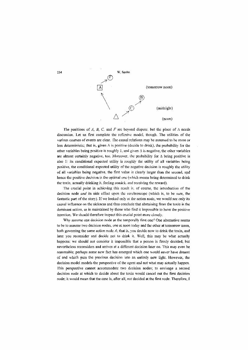
234 W, Spohn

^FA] (tomorrow noon)

\ ®

\ ^\ (C) (midnight)

A-^/—1 (noon)

The positions of A, B, C, and F are beyond dispute, but the place of A needsdiscussion. Let us first complete the reflexive model, though. The utilities of thevarious courses of events are clear. The causal relations may be assumed to be more orless deterministic; that is, given A is positive (decide to drink), the probability for theother variables being positive is roughly 1, and given A is negative, the other variablesare almost certainly negative, too. Moreover, the probability for A being positive isalso 1: its conditional expected utility is roughly the utility of all variables beingpositive, the conditional expected utility of the negative decision is roughly the utilityof all variables being negative, the first value is clearly larger than the second, andhence the positive decision is the optimal one (which means being determined to drinkthe toxin, actually drinking it, feeling seasick, and receiving the reward).

The crucial point in achieving this result is, of course, the introduction of thedecision node and its side effect upon the cerebroscope (which is, to be sure, thefantastic part of the story). If we looked only at the action node, we would see only itscausal influence on the sickness and thus conclude that abstaining from the toxin is thedominant action, as is maintained by those who find it impossible to have the positiveintention. We should therefore inspect this crucial point more closely.

Why assume one decision node as the temporally first one? One alternative seemsto be to assume two decision nodes, one at noon today and the other at tomorrow noon,both governing the same action node A; that is, you decide now to drink the toxin, andlater you reconsider and decide not to drink it. Well, this may be what actuallyhappens; we should not consider it impossible that a person is firmly decided, butnevertheless reconsiders and arrives at a different decision later on. This may even bereasonable; perhaps some new fact has emerged which one would never have dreamtof and which puts the previous decision into an entirely new light. However, thedecision model models the perspective of the agent and not what may actually happen.This perspective cannot accommodate two decision nodes; to envisage a seconddecision node at which to decide about the toxin would cancel out the first decisionnode; it would mean that the case is, after all, not decided at the first node. Therefore, I

Dependency Equilibria 235think condition (2) is right in insisting that each action node is governed by exactly onedecision node.

Are there any further alternatives? I see only one, namely, to place the decisionnode A immediately before the action node A. My condition (2) above allows for anytemporal distance between an action node and the relevant decision node. This isperhaps too liberal. It might be tempting to think that as long as there is time to decideabout an action, it is not yet decided; this would imply that the decision to do a islocated immediately before a, and hence A immediately before A. But I am nottempted by this idea. I do not see why one should exclude the possibility to decide amatter very early, to maintain one's decidedness until the time of action has come, andthen to do what one has decided. One may object that maintaining one's decidedness isa matter of choice, something one may or may not do. Perhaps. But then we are back atthe first alternative, which we have already rejected. Again, one has to distinguishbetween an external, objective perspective and the agent's intentional perspective.Objectively, the agent always has a choice - I do not see why I should deny this - sothat the matter is decided only at the last possible moment. By contrast, from theagent's present point of view, there can be only one choice: either right now, and thenit is a matter of intention to stick to that choice; or later on, and then it is a matter ofprediction what the situation and the choice will be. And it is the agent's point of viewwhich is to be captured by our modeling.

Part of the present intention or decision to do a some time later is the intention notto reopen the issue in the meantime. This intention and the capability to realize it maybe subsumed under the label "commitment power".42 More or less of this power maybe needed. We shall soon see that the same point will be relevant to Newcomb'sproblem and that the commitment power needed there is minimal. In the case ofUlysses and the Sirens the required commitment power is superhuman; intention andwill is powerless against the seduction of the Sirens; and knowing this, Ulysses iswell-advised to have the sailors' ears blocked and let himself be bound to the mast,The toxin case is between the extremes; it takes some courage to resist the temptationand to overcome the disgust. Of course, to some extent it is vague and, I suspect, evena matter of convention when the intention is (too) feeble and the temptation (too)

"One must be careful here. „Commitment" is rather a family concept in game theory. Each specificapplication is clear, but what unites the various applications is not entirely clear. However, oneprevailing idea seems to be that in order to be committed to do a, I have to commit myself to do a,where the latter is an action by which I establish external forces, as it were, that will compel me to doa. In this sense, commitment power is the power to establish such external forces. In my view, acommitment can exist without such externalization (even though this is sometimes characterized asmagic or self-hypnosis), and in this sense, commitment power is, as explained, the capability tomaintain one's decidedness (which may, of course, be supported by external means). McClennen(1990, sects. 9.7 and 12.9) has best explained the meaning of „commitment" as I am using it.

236 W.Spohnstrong, that is, when the weakness of the will is or is not exculpable. And thisvagueness can, of course, not be resolved by the cerebroscope. It is an unavoidable,not a central aspect of the above example.

It should be clear by now that the distinction I am belaboring here is tantamount tothe distinction between sophisticated and resolute choice by McClennen (1990).Sophisticated choice takes a predictive attitude toward future actions and optimizespresent actions given the predictions. Resolute choice, by contrast, takes an intentionalor commissive attitude toward future actions and optimizes present and future actionsat once. Like McClennen I find nothing miraculous in that intentional attitude ofresolute choice. Hence, it is a welcome aspect that the distinction is reflected in myformal framework. But the way in which it is reflected is perhaps more important,namely simply by the temporal location of the decision node(s) in the reflexive model.Reflexive decision theory is thus able to reconcile these two methods of choice; theyare both instantiations of one kind of model and one decision rule.

Indeed, there is a choice here between sophisticated and resolute choice.Obviously it is not fixed in advance at which time the decision node A is to be located.You may decide the case right now, or you may defer the decision to tomorrow. Andyou choose when to decide according to where you have the higher conditionalexpected utility. In the model presented above it is higher than in the model where A islater. Thus, in the above reflexive model of the toxin puzzle I have already specifiedthe result of this optimization. Hence, whether the agent proceeds according tosophisticated or to resolute choice, is itself a matter of optimal choice. Reflexivedecision models do not yet represent this choice since they assume a fixed causalgraph. But they show a way to extend the theory so as to cover this choice as well.This extension would be most interesting, but it is beyond the scope of this paper, allthe more so as we have left the general decision rule for reflexive decision modelsaside.

5.2 Newcomb 's problem

With all these points in mind let us turn now to Newcomb 's problem which is muchcloser to our ultimate concern since it bears often observed similarities to theprisoners' dilemma. The problem is quickly explained:

You will be led into a room with two boxes on the table. One is transparent andvisibly contains $ 1,000; the other is opaque, but you are told that it contains either $ 0or $ 1,000.000: You have a choice: you may take either the opaque box only (one-boxing) or both boxes (two-boxing). This seems an easy choice - of course, you do notwant to miss out on the additional thousand dollars in the transparent box - but there isa highly irritating detail. A predictor has already predicted what you will do and has

Dependency Equilibria 237filled the opaque box accordingly. If her prediction is that you will take only one box,she fills it with a million dollars; if she predicts you will be two-boxing, nothing is putinto the opaque box. As I mentioned, the prediction and the filling of the boxes arealready completed; any cheatful change is excluded. The predictor is surprisinglyknowledgeable, and you know this. In, say, 95 percent of the cases her prediction iscorrect, concerning one-boxers and two-boxers alike; and very likely she will becorrect in your case as well. Does this story behind the opaque box change your mind?Will you now take only one box?

The majority tends to stick to two-boxing, and there is a considerable variety oftheories justifying this." I find the simplest theory emerges when we look at the naturalformalization of the situation in a basic decision model, which contains threevariables; the action variable B = {one-boxing, two-boxing}, and two occurrencevariables P = {prediction of one-boxing, prediction of two-boxing}, R (= return) ={receiving $ 0, $ 1,000, $ 1,000,000, $ 1,001,000}. The temporal, and thus the causal,relations are clear:

®

^ \

®

You cannot influence the prediction because it has already taken place, and evenin a reflexive context the prediction cannot influence your decision because you haveno information whatsoever about it. The point now is that the agent's probabilitieshave to agree with this causal graph. Hence, the prediction is not only causally, but

"See, e.g., the papers collected in Campbell, Sowden (1985) and Sobel (1994), and, more recently,Joyce(1999).

238 W. Spohnalso probabilistically independent of your choice4'1, and so two-boxing turns out as thedominating action and as the only rational choice."

For more than twenty years I was firmly convinced by this consideration. Butnagging doubts have kept returning. It is not only that the minority of one-boxers is thepersonified bad conscience of the majority of two-boxers.4' Rather, it is the question ofGibbard and Harper (1978): "If you're so smart, why ain'cha rich?" The answer ofLewis (1981) is that rational persons have no chance if irrationality is (pre-)rewarded.But this answer is feeble-minded; somehow rationality should show in the adaptabilityto the conditions of success.

The doubts are reinforced if we look at the iteration of Newcomb's problem.Suppose you are confronted with this situation a hundred times, say, once a day for ahundred days. So, if all goes well, you will have earned a hundred million dollars! Butit seems you cannot earn them; backward induction stands against it: The above modelapplies to the last round; hence you will decide then to take both boxes. If the predictordoes not have a false theory about you, she will predict exactly this, and you willreceive just one thousand dollars. Thus, it is clear already now what will happen in thelast round, and since this is clear, the only rational thing for you to do in thepenultimate round is again to take both boxes, and so forth. On the whole, you willthus end up with a hundred thousand dollars instead of a hundred million. This seemsabsurd.

Of course, one should scrutinize this use of backward induction. Perhaps it is moreproblematic here than in the genuine game theoretic application (though I do not seewhy). However, despite the doubts that have been raised against backward induction, itis a forceful argument.4' Therefore, I think it would be too weak a strategy only to tryto undermine backward induction. Indeed, the absurdity is also created by the claimthat only two-boxing is rational in the one-shot case. This claim was doubtful as well.Hence let us look more carefully at the original problem.

"This entails that you cannot transfer the predictor's observed success rate of 95 percent to your owncase and form the corresponding probabilities conditional on your own options. That this divergencebetween the statistical and the subjective probabilities in your own case lies at the heart ofNewcomb's problem was forcefully argued by Kyburg (1980)."This is the view of Newcomb's problem which I have presented in Spohn (1978, sect. 5.1). It isexplained also in Meek, Glymour (1994) with the explicit use of the theory ofBayesian nets."'Jeffrey, for instance, has changed his mind several times, in (1983), (1988), and (1996)."The doubts were initiated by Binmore (1987), Reny (1989), Bicchieri (1989) and Pettit, Sugden(1989). Aumann (1995) proves backward induction to be valid under certain assumptions. This resultmay be used as a defense of backward induction (against Aumann's explicit advise). However,Rabinowicz (1998) in turn makes clear the respect in which these assumptions are unreasonablystrong. Rabinowicz is right, I think, but the gap he opens seems too small to accommodate all thepositive conclusions about cooperation I am after.

Dependency Equilibria 239Let us start by asking what you might or should think about the predictor, if you

were in this situation. No doubt you would be wondering how she manages to be sosuccessful and what her theory about human agents might be. On the other hand, it isclear what your own theory about yourself is. You firmly believe to be rational and tomaximize conditional expected utility. This is how you fix your intentions concerningyour present actions, and this is how you predict your future actions in futuresituations. That this is so is, of course, presupposed in this paper. If your self-theory isentirely different, this paper simply does not apply to you.

These remarks do not yet fully determine your self-theory since maximizingconditional expected utility may mean various things explicated in a number oftheories that differ in certain details. We will come to this in a moment. What I want tofocus on right now is the tension between your assuredness regarding your self-theoryand your bewilderment about the predictor. Perhaps the predictor has simply beenlucky to have been successful so many times in the past; but this is too improbable.Perhaps her prediction is guided, say, by the form of your nose and thus by an entirelywrong theory; but again success with such a theory appears to be sheer luck. Thus, inview of your self-theory, you should rather assume that her means of prediction arecorrelated not only with your action, but also with your ways of deciding and thuscausing the action. Thereby you do not assume a mystery. Ideally, the predictor'stheory about you should be the same as your self-theory. This ideal is not so difficult toattain; after all, we are here publicly discussing your self-theory. And certainly, youwould like this ideal to obtain; you cannot believe that there is any better theory aboutyou than your self-theory.

Now, whatever the predictor's precise thoughts, there can only be a correlationbetween her prediction and your decision, either if one causally depends on the otheror if both have a common cause; that is what Reichenbach's principle of the commoncause tells us." The case that your decision causally depends on the predictor'sprediction is to be excluded from your point of view. Hence, two possibilities forreflexively modeling the decision situation remain which are depicted in the followinggraphs:

"In our context the principle says that if two variables are probabilistically dependent, then either onecausally depends on the other or there are variables on which both causally depend. In this form theprinciple follows easily from the theorem about d-separation in section 3.1.

240 W. Spohn

® ®^ \ ^ ^

@ \ E \\ \ t \

^^ A^ ^A ^ ®

(a) decision causes prediction (b) decision and prediction havea common cause

Case (b) shows how the situation was conceived by Eells (1982, p. 211), who wasthe first to introduce the reflexive point of view, and how thereafter the correlationbetween prediction and action was usually understood. If we look here at the reducedand truncated model §o 6 A, which is reflected by the full model 5, we find that B andP, action and prediction variable, are causally and probabilistically independent.Hence, two-boxing is the dominant and thus optimal action in So and in S as well.

Fisher's smoking scenario has the same structure as case (b) provided the arrowfrom P to R is deleted. Here, X would be the variable of the smoking gene that isresponsible for the desire to smoke as well as for lung cancer, P would representgetting lung cancer, B would be the action variable about smoking, R would be avariable about the pleasure derived from smoking, and A would be the decisionvariable containing the various possible desirabilities for smoking caused by X. Then,as before, if I find myself in the actual decision situation 5o with its preference forsmoking, it would be rational to smoke since it is causally and probabilisticallyindependent from P and thus dominates nonsmoking.

So, am I wedded to familiar views? No. Case (a) is a possible scenario as well,making even more sense and allowing very different conclusions; this is what I wouldlike to defend in the following. Case (a) presupposes that the decision variable Atemporally precedes the prediction variable P. This seems to contradict the verydescription ofNewcomb's problem; here you are standing before the two boxes, andnow is the time to decide. However, we have observed in the toxin puzzle that thetemporal position of the decision variable is something that is within your choice, too.Thus, when you are standing before the boxes, you may as well consider the decisionas having been taken a long time ago and as having only to be executed right now.Indeed, it would be rational to place the decision variable at such an early time becausethis yields the higher conditional expected utility. And, although it may be unclear how

Dependency Equilibria 241the predictor actually arrives at her prediction, it follows that, if she has observed yourrationality in the past and thus uses the correct theory to predict your behavior, sheshould take you to be decided to take only one box and hence put the million dollarsinto the opaque box. This leaves open the exact temporal position of A. You can placeit as early as you want, in principle as early as the inception of your rationality (but, ofcourse, this, too, is not an event with a well-defined temporal location), and in any caseearly enough for the predictor to observe, and to become convinced of, yourrationality.

What I would like to claim is that case (a) at least presents an intentional pictureyou may have. I cannot say you should have it because it is too unclear how thepredictor operates. Maybe case (b) actually applies, however early A is placed, eventhough the predictor is much more likely to observe the consequences of yourrationality rather than its causal preconditions. Maybe case (a) applies, but your trust inthe efficiency of your decidedness regarding the predictor is not firm enough to justifyone-boxing. Maybe the predictor thinks that despite being decided to take only one boxyou will succumb to the temptation to take the additional thousand dollars. Or maybethe predictor has indeed been nothing but lucky. All this is unclear. Still, case (a) is away to rationalize one-boxing without causal mystery, and if you could be sufficientlysure that the predictor has developed a correct picture of you, then case (a) providesthe optimal representation of your situation and you should be decided to take only onebox.

According to this point of view, the presentation ofNewcomb's problem has beenutterly deceptive. It was presented as if you had to decide now so that the causalsituation could only be as in case (b). But actually you can also consider yourself to bedecided so that now, when standing before the boxes, you simply have to carry outyour previous commitment without being in a new decision situation.

All this shows, by the way, the difference to the smoking gene example. There isno way to conceive that example as in (a) and thus to rationalize nonsmoking.

The same caveat applies here as in the toxin puzzle. Even if case (a) representsyour intentional picture of the situation (as it should, given you have enough trust intothe predictor), it is not a picture of what actually happens. Standing before the boxeswith the best of your intentions, you may still reopen the issue, decide anew, andconclude to take both boxes. Or you might simply succumb to the temptation to taketwo boxes (although there is no aversion to overcome in this case in order to stick toyour commitment). Or you might believe you can outsmart the predictor, and so on.Either way, you may end up taking both boxes against your rational intention.

However, let us look again at the iterated case where you have the relevant choicea fixed number of times. (An informal look will suffice, it would be too cumbersometo formalize it.) According to the old picture, case (b), backward induction showed that

242 W. Spohnyou should rationally take both boxes every time, that the predictor, if she has a correcttheory about you, should predict just this, and that your only way to circumvent thisresult is to somehow convince the predictor of your irrationality (say, by starting totake only one box). The new picture, case (a), is completely reversed. Now thepredictor should rationally expect you to take only one box; and if you are as rationalas always to take only one box, everything is fine. If, however, she observes you takingtwo boxes, this will undermine her belief in your rationality, and she will presumablyadjust her predictions. The crucial point is here that the backward induction has lost itsbase because we have shown two-boxing to be not the only rational solution of thesingle-shot case. On the contrary, if the predictor has the right theory about you, one-boxing is the only rational solution of the single-shot case. And backward inductionthen shows that this is so in the iterated case as well. At any rate, whatever yourtemptation to deviate from your rational intention in the single-shot case may be, itshould be effectively suppressed in the iterated case.

Let me make sure that the crucial step in my argument is crystal clear: It is mystipulation in section 4.3 that in the truncated reduction of the reflexive model thecausal arrows have to go from the action children of the deleted decision node to itsother children, even if the latter precede the former. This anomaly can be observed inour examples. There, the truncated reduction 60 contains an edge from B to the earlierP (Newcomb) or from A to the earlier C (toxin), respectively, and the probabilities in5o agree with this. But this does not amount to assuming backward causation. Rather,the arrow B —> P in the truncated reduction §o means only that P causally depends onB, or B and P have a common cause (since the N-case cannot apply); and the latter isindeed true of our cases. Hence, rather than creating a mystery, we have anexplanation how the probabilities can be as they are in 5o without assuming a causalanomaly, namely, by understanding these probabilities and the dependencies theyembody as the result from reducing and truncating a richer, entirely normal causalgraph.

Finally, only because the probabilities are as they are in 80, the rationality isreversed, and drinking the toxin and taking one box turn out to maximize conditionalexpected utility. In a nutshell, the point is this: (1) that we may maximize theconditional expected utility of our decision or that of our action, (2) that the twomaximizations may fall apart, (3) that in such cases only the former, i.e., themaximization of the conditional expected utility of the decision, is rational, (4) thatthis maximization can be made explicit only in a reflexive model, and (5) that it is onlythe truncated reduction of the reflexive model as here defined which preserves thismaximization on the level of unreflexive models.

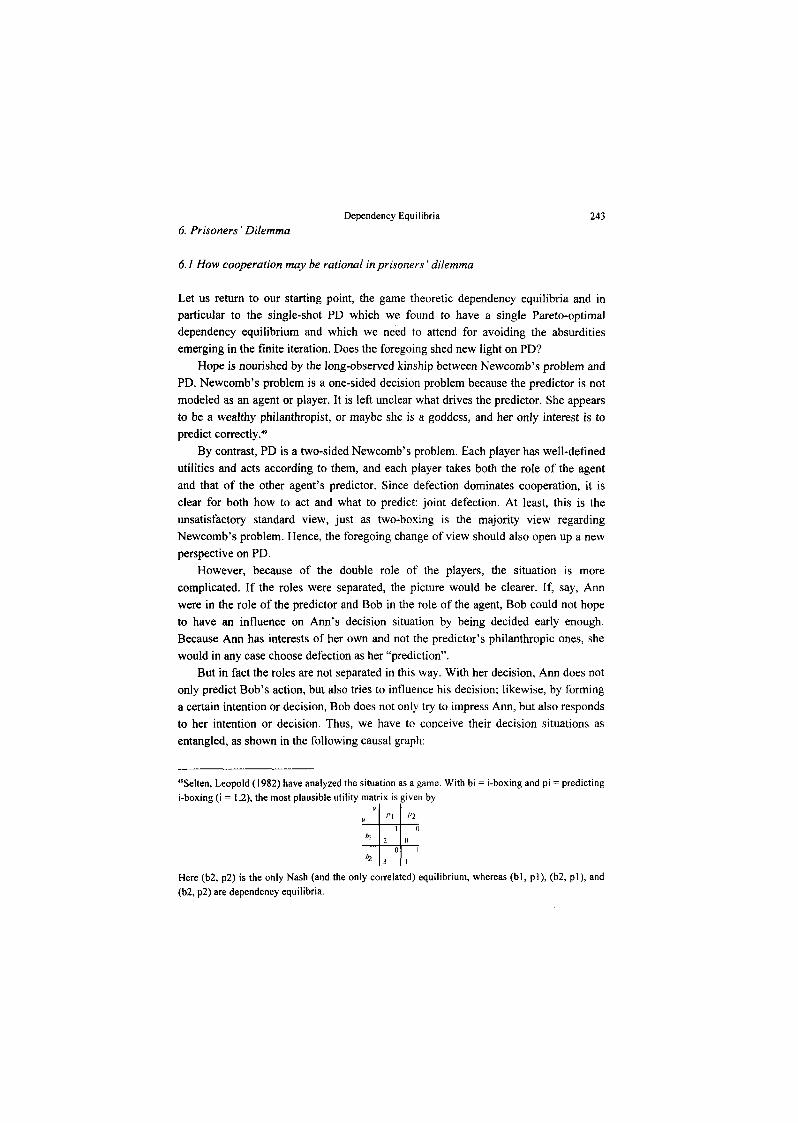
Dependency Equilibria 2436. Prisoners' Dilemma

6. l How cooperation may be rational in prisoners ' dilemma

Let us return to our starting point, the game theoretic dependency equilibria and inparticular to the single-shot PD which we found to have a single Pareto-optimaldependency equilibrium and which we need to attend for avoiding the absurditiesemerging in the finite iteration. Does the foregoing shed new light on PD?

Hope is nourished by the long-observed kinship between Newcomb's problem andPD. Newcomb's problem is a one-sided decision problem because the predictor is notmodeled as an agent or player. It is left unclear what drives the predictor. She appearsto be a wealthy philanthropist, or maybe she is a goddess, and her only interest is topredict correctly."'

By contrast, PD is a two-sided Newcomb's problem. Each player has well-definedutilities and acts according to them, and each player takes both the role of the agentand that of the other agent's predictor. Since defection dominates cooperation, it isclear for both how to act and what to predict: joint defection. At least, this is theunsatisfactory standard view, just as two-boxing is the majority view regardingNewcomb's problem. Hence, the foregoing change of view should also open up a newperspective on PD.

However, because of the double role of the players, the situation is morecomplicated. If the roles were separated, the picture would be clearer. If, say, Annwere in the role of the predictor and Bob in the role of the agent. Bob could not hopeto have an influence on Ann's decision situation by being decided early enough.Because Ann has interests of her own and not the predictor's philanthropic ones, shewould in any case choose defection as her "prediction".

But in fact the roles are not separated in this way. With her decision, Ann does notonly predict Bob's action, but also tries to influence his decision; likewise, by forminga certain intention or decision. Bob does not only try to impress Ann, but also respondsto her intention or decision. Thus, we have to conceive their decision situations asentangled, as shown in the following causal graph:

"Selten, Leopold (1982) have analyzed the situation as a game. With bi = i-boxing and pi = predictingi-boxing (i = 1,2), the most plausible utility matrix is given by

„ " r\ "2l o

*1 2__00 l

^ 3 l

Here (b2, p2) is the only Nash (and the only correlated) equilibrium, whereas (bl, pi), (b2, pi), and(b2, p2) are dependency equilibria.

244 W.Spohn

®^ u^

B Bt tA <——> A

Here, AA and 5 are occurrence nodes from Ann's perspective; her decision node isonly A„ and her action node is only A. The converse holds for Bob.

By drawing a double arrow between An and A», I have enriched causal graphs in away initially not allowed. How are we understand this double arrow? Not as a causalloop, which would be impossible. I think we should rather conceive the variables Agand A;, as temporally extended so that there is enough time for causal influence to flowback and forth and thus to establish the interdependence indicated by the double arrow.Hence, there is no causal mystery here.

However, by assuming this interdependence, have I not violated the independenceconstitutive of PD outright? No, I do not think so. The independence in PD applied tothe actions, in the first place. And this holds here as well; there is no causal influencerunning from A to B or from B to A.

That is a lame argument, one will object; of course, the causal independence wasalso meant to hold between the players' decision situations. There the criminals sit intheir prison cells, pondering what to do and being firmly precluded from anycommunication. Well, one may represent their situation in this way; then one wouldhave to delete the double arrow in the diagram above, and joint defection would ensueas the only rational solution.

But one need not represent their situation in this way. My point here is the same asin Newcomb's problem, where one could take one's decision as having beendetermined a long time before one is actually standing before the boxes. The temporallocation of the decision was not fixed there; rather, it was rational in the sense ofmaximizing conditional expected utility to locate it as early as possible.

Likewise in PD, I am not simply referring to the trivial fact that the criminals mayhave communicated and coordinated long before they were imprisoned and that lateron they may stick to their old intentions or decisions. I rather think that the playersshould see their decision situations, even in the absence of communication, as beingentangled in the way described above, and that this entanglement can rationally takeonly the form of the Pareto-optimal dependency equilibrium since this is the only wayhow they can individually(!) maximize conditional expected utility. This is what full

Dependency Equilibria 245rationality demands for all PD-like situations; anything else but cooperation would bea deviation from full rationality, i.e., irrational.

However, it should be clear again that all this only describes how the playersshould rationally view and decide their decision situations. What actually goes on maybe different. A player may doubt that the co-player(s) are fully rational in the senseexplained (perhaps because it is likely that they have not fully grasped the theory ofrationality developed here), and he may thus have different conditional probabilitiesand different expected utilities. Or he may be tempted, against his or her intention ordecision, to reconsider the issue and conclude to defect (or not to drink the toxin, or totake two boxes), and there may be strong incentives to do so. And so on. But this doesnot disprove the rationality of cooperation.

I grant that such factors may make cooperation unlikely in the one-shot PD. Thesituation changes, however, in the iterated PD. Here, the rationality of the playersbecomes more clearly observable. In particular, if one player defects, this displays hisdeficient rationality, with all the detrimental effects on the conditional probabilitiesand future cooperation. Of course, this is far from a theoretical treatment of theiterated PD. But it completely reverses the standard rationality account of the iteratedPD in, I find, a plausible and desirable way. The cornerstone of this reversal is, ofcourse, the different view of the one-shot case, which undermines backward inductionin favor of continued defection right at the beginning. Moreover, the reversal seems toopen up the possibility of rationalizing the intuitively compelling and experimentallyconfirmed tit-for-tat strategy and similar strategies embodying kindness andresponsiveness'", a rationalization that still seems to be wanting.

6.2 A dialogue

Incredulity and rejection was the most frequent response to my accounts of the toxinpuzzle, Newcomb's problem, and PD. It may be helpful to dramatize the central doubtsin a little dialogue between the opposing wisdom (OW), which I myself still feel verystrongly, and the daring proponent (DP), whose role I have taken here.

OW: Tobehonest,! don't believe a word of what you said.DP: I can imagine.OW: Let's return to the toxin puzzle. Here you stand the other day at noon, about todrink the toxin. Do you really want to deny that you would be better off not drinkingit?DP: Yes.OW: You're kidding.

"Cf., e.g., Axelrod, Dion (1988).

246 W.SpohnDP: No. Look! It simply does not occur to me when standing before the toxin thatI'd prefer to refrain from it. This has been clear all along. But I prefer $ 10,000 evenmore. Therefore, I decided at midnight to drink the toxin, and it was part of mydecision not to decide anew; otherwise, my decision would not have been a genuineone, and I would not have got the $ 10,000.OW: But you can decide anew, and you would be better off.DP: Yes, I can, but I shouldn't. I don't deny that you are maximizing conditionalexpected utility when you refrain from drinking the toxin. But I have given you aperfectly reasonable explanation of how I am maximizing conditional expected utility,too. I would already be satisfied if you could grant this. And these are not two differentsenses of maximization. We apply the same theory, we only differ in structuring thedecision situation. Of course, I have claimed more. I have also claimed that whatmaximizes expected utility depends on when you decide, and that if you can choosewhen to decide, you are better off in the toxin case if you decide early.OW: But the final decision is taken only immediately before the action.DP: What do you mean by "final"? Is there a decision and a final decision? No, Ithink to assume that decisions always immediately precede actions would be anunsupported and restrictive assumption. You can choose when to decide in the toxincase. By the way, often you just carry out old decisions, too.OW: But only because my present deliberation would confirm my old decision. Orbecause the decision costs are too high for always deliberating anew.DP: Are you sure these are the only reasons?OW: Well, let me ask you another question: How do you manage to maintain yourdecidedness? Somehow, you have to commit yourself.DP: What do you mean?OW: I mean you have to take some measure ensuring that you will really stick toyour decision in the end, say, by instructing a friend to return the $ 10,000 if you don'tdrink the toxin.DP: That's a point where I do not understand you at all. You present the case as ifihad to guard against my rationality and had to force myself into doing something that Iwill judge to be irrational and that I would never do in the absence of force. This is avery distorted picture of commitment. I don't have to guard against my rationality;that's almost analytic. Of course, others may not trust in my sense of commitment, andthen I may have to prove it to them by some such measure. But I don't have to proveanything to myself. No, I am committed merely by the insight into the rationality ofbeing committed. This is part and parcel of what it means to be rational. It is not amysterious or superhuman additional capacity. Whether it is rational to be committeddepends on the situation, but in the toxin case it is. Of course, there are also intricateintertemporal situations that are difficult to assess, but the toxin case is a very simple

Dependency Equilibria 247one in which the basic point stands out very clearly. What I have to guard against ismy weakness that I may not follow my insight. I admit this is often necessary, butthat's another story.OW: Hm, we could be moving in circles here. Let me turn to Newcomb's problem.You have added another mystery here. In the toxin case, you actually decide bymidnight and think you can maintain this decision. In the Newcomb case, you standbefore the boxes, you reflect on the case for the first time in your life, and now you sayyou discover, as it were, that there is nothing to decide, that you have been decided fora long time, and that you only have to carry out your old commitment. How can you bedecided, when you never reflected on the case?DP: I agree, this sounds odd, at least if you conceive of a decision as an occurringmental event. But if you don't, you may well discover that you are committed. Since Ihave not pondered about Newcomb's problem before, the idea cannot be that thepredictor somehow observed me pondering and deciding to take only one box and thatshe filled the opaque box accordingly. The idea is rather that the predictor has hadmany opportunities to observe my rationality in general, that she inductively infers thatI will behave rationally on other occasions as well, that rationality, i.e., maximizingconditional expected utility as explained, requires me to be committed in this veryspecial type of situation, and that knowing this both of us behave accordingly. Thesame applies to the toxin case, by the way. If I am rational, the predictor'scerebroscope should see this, and then we both can deduce that I have the intention todrink the toxin. If you accept my toxin story, it's really a small step to accept myNewcomb story.OW: Hm. But it is not a small step to PD.DP: I agree. I fear my presentation has diminished the differences. On the otherhand, if what I said so far is acceptable, this must have consequences for PD. Do youhave something particular in mind?OW: Several things! First, you have extensively explained why the probabilities asthey are in your dependency equilibria need not imply a causal interdependencebetween the players' actions. The interdependence may as well obtain only betweentheir decision situations. Now I can imagine how the latter interdependence comesabout by all kinds of signaling, commitment moves in my sense, or what have you. Butif I understand you correctly, you allow for such things, but you say they are notrequired.DP: Yes, precisely.OW: But how am I then to conceive ofthat interdependence? That's definitely a stepbeyond your wft-opersonal "discovery to be committed".DP: Yes, certainly. But if photons can be entangled, why should persons not manageto be so as well?

248 W.SpohnOW: Come on, that's a bit farfetched, isn't it?DP: Ah, you know well enough that I would never make any quick inferences fromthe quantum to the human domain, say, from uncertainty to freedom. No, purely fromthe perspective of a theory of causation the comparison is not so farfetched. But youare right, just as I said that rationality requires you to be committed in the toxin and theNewcomb case, I now say that rationality requires both players to be entangled in thePareto-optimal dependency equilibrium and to be committed to cooperation. Thisentanglement and commitment emerges with the situation without requiring bindingagreements or whatever. That's what maximizing conditional expected utility dictates.OW: This sounds as if the players should choose their beliefs so as to maximizeconditional expected utility.DP: No, certainly not. They do believe in common rationality, and this belief hasconsequences.OW: All this is hard to believe. But let's grant your entanglement of the players'original decision situations. Now, however, my very first doubt returns. Suppose youare one of the prisoners, you are in prison, and you find yourself entangled with yourpartner, as you describe it. But you are free to break the entanglement, and you shouldnotice that you are better off by doing so. So, you should break it and leave your co-player in her imaginary entanglement. Or rather, you should realize that the same holdsfor your co-player, and that there is no way to save the entanglement, anyhow.DP: I feared that you would come up with the hardest question of all. I see the dif-ference to the toxin and the Newcomb case. There I am committed to myself. I wouldnot maximize expected utility, if I were not fully decided early enough. In PD, bycontrast, I am committed to my co-player (as she is to me), and by breaking mycommitment, I am harming her, but not, it appears, myself. That makes a difference.On the other hand, if there are commitments in the sense I have described above, whyshouldn't there be joint commitments in the same sense, whose violation would beindividually irrational?OW: ???DP: Look, I need not defend the view that cooperation is the only rational option inthe single-shot PD. The only point I want to insist upon is that one may represent thedecision situations of the players as originally entangled in the weakly Pareto-optimaldependency equilibrium - an entanglement, which is not broken by laterreconsideration and by a new decision and in which it is rational to cooperate even inthe single-shot case. That's all that is required for breaking the force of backwardinduction. As soon as you look at iterations the joint commitment will unfold itsmomentum.OW: Hm, I would like to see this worked out. But what does commitment andentanglement help in case of several Pareto-optimal dependency equilibria?

Dependency Equilibria 249DP: Not much. PD is particularly simple insofar as entanglement alone alreadyyields a unique solution. But the problem of selecting from multiple equilibria existshere as elsewhere. The rich literature on bargaining theory should apply in my settingas well as in the usual one.OW: Let me ask you a final question. By calling your dependency equilibria equilibria,you use a venerable name. This seems to be a false pretense. Equilibria are so calledbecause they are self-stabilizing. This is true of correlated equilibria as well. But Idon't see how this characterization should apply to dependency equilibria.PD: I don't find much of a difference. First of all, you know well enough that mixedNash equilibria are not self-stabilizing as such.OW: Yes, of course, they have to be backed up by Harsanyi's (1973) account, say,according to which they are approximations of equilibria in perturbed games.PD: I admit I have not thought about a similar account for mixed dependencyequilibria. But a pure dependency equilibrium is self-stabilizing. Both players have anincentive to stick to it since each would lower their conditional expected utility bydeviating from it. But even in a mixed dependency equilibrium, just as in a mixedNash equilibrium, the players don't have an incentive to deviate, in the sense that eachwill do only what has positive probability in the relevant marginal of the jointprobability distribution. Otherwise, they would again lower the conditional expectedutility.OW: But this is just the argument why correlated equilibria are self-stabilizing.DP: No, in correlated equilibria deviation includes the break of the dependency inthe equilibrium distribution. That's not the sense appropriate for dependencyequilibria. There, deviation has to keep within the entanglement of the players'decision situations, as embodied in the equilibrium distribution. Hence my consistenttalk of maximizing conditional expected utility. Of course, this is to say that thisexplanation of self-stabilization presupposes all my stories about joint commitmentand entanglement. If you don't swallow the latter, you can't accept the former.OW: You seem to have, or want to have, an answer to every question.PD: This is my role here, isn't it?OW: But roles aside, do you really believe every word you say?PD: How do you expect me to respond? I have grown up in the same tradition asyou. It is a good and strong tradition, but presumably not one with which one can befully content, and certainly not one from which one can easily free oneself. How can Iknow then what I really believe?

250 W,Spohn6.3 Some comparative remarks

So many pages have been filled with PD, indeed so many pages at least resemblingmine in spirit, that I cannot aim here for any completeness in my comparative remarks.In fact, I do not have an argument with similar approaches. The question is not reallywho is wrong and who is right, but rather to which extent the various approaches are atleast illuminating. Hence, my concluding comparative remarks rather aim at clarifyingin which way I believe my ideas to differ from similar ones.

(1) Some philosophers may say that they have offered a much simplerrationalization of cooperation in the one-shot PD than the one I have put forward,namely, via the so-called mirror principle5' which says that whenever Ann and Bob arein the same decision situation, they act in the same way. In PD they are in the samesituation because of the symmetry of the story. Hence, only joint cooperation and jointdefection are possible outcomes. If they believe in the principle, they also believe thatthese are the only possible outcomes. Hence, since for both joint cooperation is betterthan joint defection, it is rational for both to cooperate.

This argument is entailed by my account, so I agree with its conclusion. But it istoo quick. It avoids causal considerations, and it does not present a theory ofrationality that would entail the rationality of cooperation for Ann and Bob in theirparticular situation. Therefore, it does not exclude that mutual defection satisfies themirror principle as well, as the standard theory has it. In a way, it takes its conclusionfor granted. By contrast, my account tries to back up the mirror argument by specifyinga theory of rationality in which the rationality of cooperation emerges as a conclusion.Moreover, it is hard to see how to apply the mirror principle when the situation is notsymmetric; but there is no such presupposition in my account.

(2) In a similar spirit, some game theorists may say that my account really belongsto cooperative game theory within which the cooperative solution ofPD is no mystery,anyway. However, if we follow Osborne, Rubinstein (1994, pp. 255f.) and takecooperative game theory to refer to groups of players without considering "the detailsof how groups of players function internally", this is not true. I have at least attemptedto offer a theory of individual rationality rationalizing cooperation. If instead wefollow Harsanyi, Selten (1988, p. 1) and "define cooperative games as those permittingenforceable agreements", it is again not true. Clearly, my rationalization of cooperationrefrained from alluding to enforceable agreements. Whether it succeeded is, of course,another question. In any case, I have tried to tell a story about individual rationalitybacking up cooperative game theory to some extent.

(3) To continue on the issue, Harsanyi, Selten (1988, pp. 4ff.) showed howcooperation can emerge as an ordinary Nash equilibrium in a non-cooperative PD by

"Cf. Davis (1977) and Sorensen (1985).

Dependency Equilibria 251adding a preplay of commitment moves. Ann starts making her conditionalcommitment move ("I commit myself to cooperate, if Bob does so as well"). Bobfollows with his unconditional commitment move ("I commit myself to cooperate"),and then both cooperate. Thereby we do not even have to assume a causalinterdependence of the players' decision situations; the dependence is successivelygenerated by the commitment moves. We also find the relevant conditional beliefs intheir original decision situations, which turn into unconditional beliefs in cooperationafter the commitment moves have been taken. But, of course, the idea ofHarsanyi andSelten is that there is some external mechanism sufficiently lowering the pay-offs incase the commitments are violated. As I have explained, this is not my conception ofcommitment, I hoped to do without such a mechanism. Only in this way can I hope toextend my argument to the iterated PD in which cooperation should emerge withoutexternal help, an argument that has not been pursued by Harsanyi and Selten.

(4) My proposal closely resembles the old theory of conjectural variations."Friedman (1983, p. 107) concludes that "at the level of simultaneous decisions in asingle-period model, conjectural variation is not meaningful" and hence interprets theold single-period models of conjectural variation as being implicitly about a dynamicalprocess that has been more recently treated in multiperiod models. So, does this verdictapply as well to the account offered here? Yes, at least according to opposing wisdom,as I called it. However, the effective objection has been that single-period conjecturalvariations assume a causal dependence that does simply not exist. This objection doesnot apply here. At least I have taken pains with explaining why dependency equilibriado not assume the causal dependence they seem to assume. Whether my resort helpsmaking sense of the theory of conjectural variations is, however, beyond my judgment.The answer may very well be negative. After all, duopoly and PD are quite differentchapters of game theory.

(5) Without doubt, my closest allies are Albert, Heiner (2001) and Heiner, Albert,Schmidtchen (2000). They also seek a causally unassailable rationalization of one-boxing in Newcomb's problem, and they also generalize their account to a treatment ofthe single-shot PD. It is surprising to see, however, how intentions can be so close andhow their realizations can still differ in so many details. Hence, some comparativeremarks are called for.

There is no doubt that their approach is more detailed and makes sense moreimmediately. This is so because they choose quite a different setting, namely, that ofevolutionary game theory. Their idea is that solvers of Newcomb's problem come intwo types, the greedy type and the temptation resistant type. These labels are used justfor illustration, the real difference between the types lies in their decision rules. Thegreedy type bases their calculation of expected utilities on the disconnection principle,

"As Max Albert has pointed out to me. This theory is well reviewed in Friedman (1983, sect. 5.1-2).

252 W.Spohnas they call it, which favors two-boxing, and the temptation resistant type on thebacktracking principle favoring one-boxing. Moreover, the types are somehowpredictable; they send out some kind of signal which displays their type (more or lessreliably) and which the predictor can use for her prediction. It is plausible then, andAlbert and Heiner explain this more rigorously, that only the temptation resistant typewill survive if evolution rewards high pay-offs. A similar, though more complexaccount applies to PD. The players come in various types, exchanging signalsdisplaying their type, and behaving according to their type and the signal received.Then, again, evolution will favor the (conditionally) cooperative type.

At face value, at least, this is not a story about individual rationality. And it seemsit cannot be turned into one. I am lucky, or not lucky, in the evolutionary lottery thatassigns a type to me, but the question of which type I should rationally adopt does notarise. This is certainly a major difference to my attempt, and I do not see how it couldbe bridged."

A number of further differences are entailed by this. Also considering the causesof actions, Albert and Heiner introduce what they call motivation packages, whichresemble my decision nodes. However, they do not engage in what I have calledreflexive decision theory. The causal picture they develop is that of the externaltheorist rather than that of the agent himself, a fact that shows up also in their rejectionof my (or rather Bells') reflexive condition (5) in section 4.3. Indeed, a motivationpackage in their sense does not only consist of beliefs and desires or probabilities andutilities, but also of a decision criterion, and their point is that the types may differ onlyin the latter component of their motivation packages. By contrast, I have no place forvariation here. For me, there is only one decision rule, the rational one (at least as longas I have not given up and acquiesced in many rationalities). And since I am dealingonly with rational subjects, there is only one decision rule for the subjects as well.Still, I can mimic the types of Albert and Heiner. The temptation resistant (or, as Iwould say, the commissive) type is decided early, whereas the greedy type is decidedlate (though both types apply the same decision rule). And because I can decide whento be decided, I can choose my type. However, this is not to say that my commissivetype follows their backtracking principle. My account rather proceeds in terms oftruncated reductions as explained, which agrees with the backtracking principle in theNewcomb case, but perhaps not in general. Moreover, since my idea is that there is aunique rationality, I may hope to dispense with signals (though, of course, they arehelpful in actual life as well as in the presentation of models). The common insight ofthe predictee and the predictor (in the Newcomb case) or the players (in PD) into what

"In private communication Max Albert tells me they need not stick to the evolutionary approach andcould turn their story into one about individual rationality. This would indeed shift the discussionlines between us.

Dependency Equilibria 253is rational in their kind of situation should suffice. But I grant that this may be amysterious part of my account, a part Albert and Heiner cannot share, all the more so,

, as they would certainly reject my conception of commitment.Thus, I have listed seven or eight differences, and there may be more. This strikes

me as rather fruitful. It would be palliative to say that these differences confirm ourcommon intention. But they certainly span a fascinating field of further investigationthat may produce still better rationalizations of cooperation.

References

Albert, M. and R.A. Heiner (2001), "An Indirect-Evolution Approach to Newcomb's Problem",Homo Oeconomicus, forthcoming.

Aumann, R. (1974), "Subjectivity and Correlation in Randomized Strategies", Journal ofMathematical Economics 1, 67-96.

Aumann, R. (1987), "Correlated Equilibrium as an Expression of Bayesian Rationality",Econometrica 55, 1-18.

Aumann, R. (1995), "Backward Induction and Common Knowledge of Rationality", Games andEconomic Behavior 8, 6-19.

Axelrod, R. and D. Dion (1988), "The Further Evolution of Cooperation", Science 242, 1385-1390.Barwise, J. (1990), "On the Model Theory of Common Knowledge", in: J. Barwise, The Situation in

Logic, CSLI Lecture Notes 17, Cambridge 1990.Bicchieri, C. (1989), "Self-Refuting Theories of Strategic Interaction: A Paradox of Common

Knowledge", Erkenntnis 30, 69-85.Binmore, K. (1987), "Modelling Rational Players, Part I", Economics and Philosophy , 179-213.Campbell, R., L. Sowden (eds.) (1985), Paradoxes of Rationality and Cooperation, University of

British Columbia Press, Vancouver.Cartwright, N. (1989), Nature 's Capacities and Their Measurement, Oxford: Clarendon Press.Cartwright, N. (1999), "Causal Diversity and the Markov Condition", Synthese 121, 3-27.Davidson, D. (1971), "Agency", in: R. Binkley et al. (eds.), Agent, Action, and Reason, Toronto:

University of Toronto Press, 3-25.Davis, L. (1977), "Prisoners, Paradox, and Rationality", American Philosophical Quarterly 114, 319-

327.Dawid, A.P. (1979), "Conditional Independence in Statistical Theory", Journal of the Royal

Statistical Society, Series B 41, 1-31.Eells, E. (1982), Rational Decision and Causality, Cambridge: Cambridge University Press.Fishbum, P.C. (1964), Decision and Value Theory, New York: Wiley.Frank, R.H. (1988), Passions Within Reasons, New York: Norton & Company.Friedman, J.W. (1983), Oligopoly Theory, Cambridge: Cambridge University Press.Gibbard, A. and W.L. Harper (1978), "Counterfactuals and Two Kinds of Expected Utility", in: C.A.

Hooker, J.J. Leach and E.F. McClennen (eds.), Foundations and Applications of Decision Theory,vol. 1, Dordrecht: Reidel, 125-162.

Haaveimo, T. (1943), "The Statistical Implications of a System of Simultaneous Equations",Econometrica 11, 1-12.

254 W.SpohnHammond, P. (1976), "Changing Tastes and Coherent Dynamic Choice", Review of Economic Studies

43,159-173.Hammond, P. (1988), "Consequentialist Foundations for Expected Utility", Theory and Decision 25,

25-78.Harsanyi, J.C. (1973), "Games with Randomly Disturbed Payoffs: A New Rationale for Mixed

Strategies", International Journal of Game Theory 1, 1 -23.Harsanyi, J.C., R. Selten (1988), A General Theory of Equilibrium Selection in Games, Cambridge,

Mass.: MIT Press.Heiner, R.A., M. Albert and D. Schmidtchen (2000), "Rational Contingent Cooperation in the One-

Shot Prisoner's Dilemma", unpublished manuscript,Jeffrey, R.C. (1965/83), The Logic of Decision, Chicago; Chicago University Press.Jeffrey, R.C. (1988), "How to Probabilize a Newcomb Problem", in: J.H. Fetzer (ed.). Probability

and Causality, Dordrecht: Reidel, 241-251.Jeffrey, R.C. (1996), "Decision Kinematics", in: K.J. Arrow et al. (eds.), The Rational Foundations of

Economic Behaviour, Basingstoke: Macmillan, 3-19.Jensen, F.V. (1996), An Introduction to Bayesian Networks, London: UCL Press.Joyce, J.M. (1999), The Foundations of Causal Decision Theory, Cambridge: Cambridge University

Press.Kavka, G. (1983), "The Toxin Puzzle", Analysis 43, 33-36.Kyburgjr., H.E. (1980), "Acts and Conditional Probabilities", Theory and Decision 12, 149-171.Lewis,D.(1981),"'WhyAin'chaRich?'",Afoüä 15,377-380.McCIennen, E.F. (1990), Rationality and Dynamic Choice, Cambridge: Cambridge University Press.Meek, C., C. Glymour (1994), "Conditioning and Intervening", British Journal for the Philosophy of

Science^, 1001-1021.Myerson, R.B. (1991), Game Theory. Analysis of Conflict, Cambridge, Mass.: Harvard University

Press.Nozick, R. (1969), "Newcomb's Problem and Two Principles of Choice", in: N. Rescher et al. (eds.),

Essays m Honor of Carl G. Hempel, Dordrecht: Reidel, 114-146.Osborne, M.J., A. Rubinstein (1994),^ Course in Game Theory, Cambridge, Mass.: MIT Press.Pearl, J. (1988), Probabilistic Reasoning in Intelligent Systems: Networks of Plausible Inference, San

Mateo, Ca.: Morgan Kaufmann.Pearl, J. (2000), Causality. Models, Reasoning, and Inference, Cambridge: Cambridge University

Press.Pettit, P., R. Sugden (1989), "The Backward Induction Paradox", Journal of Philosophy 86, 169-182.Pollak, R.A. (1968), "Consistent Planning", Review of Economic Studies 35, 201-208.Pollock, J.L. (1995), Cognitive Carpentry, Cambridge, Mass.: MIT Press.Rabinowicz, W. (1998), "Grappling With the Centipede", Economics and Philosophy 14, 95-125.Rabinowicz, W. (2002), "Does Deliberation Crowd Out Self-Prediction?", to appear in Erkenntnis.Reny, P. (1989), "Common Knowledge and Games With Perfect Information", Proceedings of the

Philosophy of Science Association 2, 363-393.Salmon, W.C. (1980), "Probabilistic Causality", Pacific Philosophical Quarterly^, 50-74.Salmon, W.C. (1984), Scientific Explanation and the Causal Structure of the World, Princeton, N.J.:

Princeton University Press.Savage, L.J. (1954), The Foundations of Statistics, New York: Dover,.2nd. ed. 1972.Selten, R. and U. Leopold (1982), "Subjunctive Conditionals in Decision and Game Theory", in: W.

Stegmtlller, W. Balzer and W. Spohn (eds.), Philosophy of Economics, Berlin: Springer, 191-200.Shafer,G. (1996), The Art of Causal Conjecture, Cambridge, Mass.: MIT Press.

Dependency Equilibria 255Simon, H.A. (1957), Models of Man, New York: Wiley.Sobel, J.H. (1994), Taking Chances: Essays on Rational Choice, Cambridge: Cambridge University

Press.Sorensen, R.A. (1985), "The Iterated Versions ofNewcomb's Problem and the Prisoner's Dilemma",

Synthese 63, 157-166.Spirtes, P., C. Glymour and R. Scheines (1993), Causation, Prediction, and Search, Berlin: Springer.Spohn, W. (1976/78), Grundlagen der Entscheidungstheorie, Ph.D. Thesis Munich 1976, published

at Scriptor, Kronberg/Ts. 1978.Spohn, W. (1977), "Where Luce and Krantz Do Really Generalize Savage's Decision Model",

Erkenntnis 11, 113-134.Spohn, W. (1980), "Stochastic Independence, Causal Independence, and Shieldability", Journal of

Philosophical Logic 9, 73-99.Spohn, W. (1982), "How to Make Sense of Game Theory", in: W. Stegmüller, W. Balzer and W.

Spohn (eds.). Philosophy of Economics, Berlin: Springer, 239-270; reprinted in: Y. Varoufakis andA. Housego (eds.), Game Theory: Critical Concepts, Vol. 4. Discontents, London: Routledge, 2001,213-241.

Spohn, W. (1988), "Ordinal Conditional Functions: A Dynamic Theory of Epistemic States", in:W.L. Harper and B. Skyrms (eds.). Causation m Decision, Belief Change, and Statistics, Dordrecht:Kluwer, 105-134.

Spohn, W. (1999), "Strategic Rationality", Forschungsberichte der DFG-Forschergruppe "Logik inder Philosophie". Nr. 24, Konstanz.

Spohn, W. (2000), "A Rationalization of Cooperation in the Iterated Prisoner's Dilemma", in: J.Nida-Rumelin and W. Spohn (eds.). Rationality, Rules, and Structure, Dordrecht: Kluwer, 67-84.

Spohn, W. (2001), "Bayesian Nets Are All There Is to Causal Dependence", in: D. Costantini, M.C.Galavotti and P. Suppes (eds.), Stochastic Dependence and Causality, Stanford: CSLI Publications,forthcoming.

Spohn, W. (2002), "A Brief Comparison of Pollock's Defeasible Reasoning and Ranking Functions",Synthese 131,39-56.

Stalnaker, R.C. (1999), Context and Content, Oxford: Oxford University Press.Strotz, R.H. (1955/56), "Myopia and Inconsistency in Dynamic Utility Maximization", Review of

Economic Studies 23, 165-180.Verma, T. and J. Pearl (1990). "Causal Networks: Semantics and Expressiveness", in: R.D. Shachter

et al. (eds.). Uncertainty in Artificial Intelligence, vol. 4, North-Holland, Amsterdam, 69-76.Wright, S. (1934), "The Method of Path Coefficients", Annals of Mathematical Statistics 5, 16J-215.Yaari, M.E. (1977), "Endogeneous Changes in Tastes: A Philosophical Discussion", Erkenntnis 11,

157-196.

dependency equilibria and the causal structure of … · dependency equilibria and the causal...

Documents