investigation of the pressure dependency of phase...
TRANSCRIPT

Investigation of the pressure dependency of phase equilibria in
colloidal model systems
Inaugural-Dissertation
zur
Erlangung des Doktorgrades der
Mathematisch-Naturwissenschaftlichen Fakultät
der Heinrich-Heine-Universität Düsseldorf
vorgelegt von
Karolina Tomczyk aus Zgierz
May 2011

2
Aus dem Institut für
der Heinrich-Heine-Universität Düsseldorf
Gedruckt mit der Genehmigung der
Mathematisch-Naturwissenschaftlichen Fakultät der
Heinrich-Heine-Universität Düsseldorf
Referent: Prof. Dr. J. K. G. Dhont
Koreferent: Prof. Dr. S. U. Egelhaaf
Tag der mündlichen Prüfung: 29.06.2011

3
Summary
In this thesis the experimental studies of pressure jumps effect on several systems,
representing a cross-section of soft matter materials. The phase behaviour of colloidal
dispersions and polymeric micellar solutions using temperature and pressure as variables
are presented in the first part. The second part addresses the correlation between
temperature dependency of polymer viscosity and the diffusion time of a nanoscopic
probe dissolved in this polymer.
As the first subject-matter, the interplay between percolation and phase separation
effect appearing in an adhesive hard sphere (AHS) system, represented by octadecyl
coated silica particles dissolved in toluene, is discussed. The transitions to the percolated
and the biphasic states are obtained and they are in agreement with theoretical
predictions. For concentrations higher than around 12-14vol%, the increase of the
forward scattering intensity is found to be governed by the proximity of the spinodal line.
But it is the percolation effect that controls the time scale at which the forward scattering
intensity increases. For lower concentrations two approaches to determine spinodal line
were proposed. Depending on the way of spinodal determination the system is expected
to undergo phase separation either through nucleation or spinodal decomposition process.
In the first scenario the sample starts to reveal the non-ergodic behaviour while forming
nuclei (the denser phase), and the spinodal lies below the percolation line in the phase
diagram. In the latter scenario the spinodal is expected to lie between binodal and
percolation lines, and while system is decomposing, the sample volume spanning
network is formed, which gives rise to non-ergodic behaviour attributed to the percolated
state. This is the first study of competition between percolation and phase separation
addressed with time-resolved measurement.
In the next chapter the temperature- and pressure-dependent behaviour of the
water and water-DMF solutions of polymeric micelles composed of poly(ethylene-co-
propylene-b-(ethylene oxide)) (PEP-PEO) block copolymer is described. It is found that
the micellar radius of gyration for the water solution decreases while approaching the
lower critical solution temperature (LCST), which is obtained by increasing temperature
and pressure. However, in water-DMF dispersion there is no change in micellar radius

4
until the phase separation sets in. In the first case applying pressure has similar effect as
increasing temperature (although there is no simple linear dP/dT relation), and in the
latter case it acts as lowering of temperature.
In the last part the temperature dependence of diffusion of rubrene in the
poly(ethylene-co-propylene) (PEP) polymer melt is investigated by fluorescence
correlation spectroscopy. Its correlation with temperature dependence of polymer
viscosity is found. This is a proof that the changes in rubrene diffusion while varying
temperature are solely due to temperature variation of PEP viscosity.

5
Zusammenfassung
Diese Arbeit befasst sich mit der experimentellen Untersuchung der Effekte von
Drucksprüngen in verschiedenen Systemen aus Materialien die der weichen Materie
zuzuordnen sind. Im ersten Teil werden Phasenübergängen Kolloidaler Dispersionen
sowie Lösungen von Polymermizellen untersucht, wobei Temperatur und Druck als
Kontrollparameter dienen. Im zweiten Teil werden Korrelationen zwischen
temperaturabhängiger Viskosität von Polymerlschmelzen und der Diffusion darin
suspendierter, nanoskopischer Testpartikel untersucht.
Die erste Teil der Untersuchung befasst sich mit dem Zusammenspiel zwischen
Perkolation und Phasentrennung von adhäsiven harten Kugeln, hier repräsentiert durch
Octadecyl-beschichtete, in Toluene gelöste Silica Partikel. Die gemessenen Übergänge in
den perkolierten und im zweiphasigen Zustand sind in Übereinstimmung mit
theoretischen Vorhersagen. Für Konzentrationen von mehr als 12-14vol% bestimmt die
Entfernung zur Spinodalen die Zunahme der vorwärts gestreuten Intensität. Die Zeitskala
der zeitlichen Zunahme wird durch den Perkolationseffekt bestimmt. Für geringere
Konzentrationen wurden zwei unterschiedliche Wege zur Bestimmung der Spinodalen
vorgeschlagen. Je nach Methode der Herleitung ist eine Phasentrennung durch
Keimbildung oder spinodale Entmischung zu erwarten. Im ersten Fall wird das System
bei der Bildung von Keimen der dichteren Phase nicht-ergodisch, und die Spinodale
befindet sich im Phasendiagramm unter der Perkolationslinie. Im Gegensatz dazu liegt
die Spinodale im zweiten Fall zwischen der Binodalen und der Perkolationslinie, und bei
der Phasentrennung bildet sich ein das Systemvolumen übergreifendes Netzwerk,
welches die Nichtergodizität des perkolierten Zustands verursacht.
Im nächsten Kapitel wird das Temperatur- und Druckabhängige Verhalten von
Lösungen aus Poly(Ethylen-co-Propylen-b-(Ethylen Oxid)) (PEP-PEO) Block-
Copolymeren in Wasser und Wasser-DMF Mischungen beschrieben. Bei Annäherung an
die untere kritische Lösungstemperatur durch Erhöhung von Druck und Temperatur wird
im Fall der wässrigen Lösung eine Abnahme des Gyrationsradius der Mizellen
beobachtet. Dahingegen ist der Gyrationsradius der Mizellen in Wasser-DMF
Dispersionen unverändert bis zum Einsetzen der Phasentrennung. Im ersten Fall ist der

6
Effekt einer Druckerhöhung ähnlich dem einer Temperaturerhöhung (obwohl es keine
einfache dP/dT-Relation gilt), während im zweiten Fall die Druckerhöhung einer
Verringerung der Temperatur ähnlich ist.
Im letzten Teil der Arbeit wird mittels Fluoreszenzkorrelations-spektroskopie die
Temperaturabhängigkeit der Diffusion von Rubrene in Poly(Ethylen-co-Propylen) (PEP)
Polymerschmelzen untersucht. Es zeigt sich eine Korrelation der Diffusion mit der
Polymerviskosität. Dadurch wird belegt, dass Änderungen in der Diffusion von Rubrene
bei Temperaturänderung allein durch Variation der Viskosität von PEP mit der
Temperatur zustande kommen.

7
Contents 1. Introduction..................................................................................................................... 9
2. Phase diagram of an adhesive hard sphere (AHS) system and the interplay between
demixing and percolation effects ...................................................................................... 14
2.1. Introduction............................................................................................................ 14
2.2. Experimental Section ............................................................................................. 21
2.2.1. Materials ......................................................................................................... 21
2.2.2. Experimental techniques and set-ups.............................................................. 21
2.3. Results.................................................................................................................... 28
2.3.1. Determination of the percolation line ............................................................. 28
2.3.2. Determination of the binodal line ................................................................... 31
2.3.3. Analysis of forward scattering intensity and first approach to determine the
spinodal line .............................................................................................................. 34
2.3.4. Time dependency and second approach to determine the spinodal line ......... 43
2.4. Discussion .............................................................................................................. 47
2.4.1. Phase behaviour of 16% sample ..................................................................... 49
2.4.2. First scenario of phase behaviour of low concentrated samples – phase
separation through nucleation process ...................................................................... 50
2.4.3. Second scenario of phase behaviour of low concentrated samples – phase
separation through spinodal decomposition process................................................. 54
2.5. Conclusions............................................................................................................ 55
3. Temperature- and pressure-dependent behaviour of PEP-PEO polymeric micelles in
water and water-DMF solutions........................................................................................ 57
3.1. Introduction............................................................................................................ 57
3.2. Experimental section.............................................................................................. 61
3.2.1. Materials ......................................................................................................... 61
3.2.2. Experimental techniques and set-ups.............................................................. 66
3.3. Results for dhPEP5-hPEO120 in D2O ................................................................... 77
3.3.1. SANS results ................................................................................................... 77
3.3.2. SLS and DLS results ....................................................................................... 83

8
3.4. Phase separation of dhPEP5-hPEO120 and hPEO150 systems in D2O-dDMF
solution.......................................................................................................................... 87
3.4.1. Observation of phase separation at ambient pressure conditions ................... 87
3.4.2. Observation of pressure induced phase separation ......................................... 90
3.4.3. Observation of pressure induced phase separation in solution of homopolymer
PEO150 in D2O-dDMF............................................................................................. 95
3.5. Discussion .............................................................................................................. 98
3.5.1. Temperature- and pressure-induced shrinkage of dhPEP5-hPEO120 in D2O 99
3.5.2. Temperature- and pressure- induced phase separation of dhPEP5-hPEO120
and hPEO150 in D2O-dDMF .................................................................................. 103
3.6. Conclusions.......................................................................................................... 106
4. The temperature dependence of the poly(ethylene-co-propylene) (PEP) copolymer
macroscopic viscosity studied by Fluorescence Correlation Spectroscopy (FCS)......... 109
4.1. Introduction.......................................................................................................... 109
4.2. Experimental section............................................................................................ 110
4.2.1. Materials ....................................................................................................... 110
4.2.2. Viscosity measurement ................................................................................. 111
4.2.3. Fluorescence Correlation Spectroscopy (FCS) ............................................. 112
4.3. Results and discussion ......................................................................................... 116
5.4. Conclusions and outlook...................................................................................... 121
References:...................................................................................................................... 123

9
1. Introduction
The soft matter systems are extensively studied since the beginning of the 19th
century. Soft matter is a general term describing a very large class of materials whose
common feature is that they are composed of particles with typical sizes between 1nm
and 1μm dispersed in a solvent whose molecules are much smaller in size, among which
the most important categories are colloids, polymers and amphiphilic systems [1]. In this
thesis, studies of systems representing the two first groups will be described. In the last
two decades, with the evolution of soft condensed matter physics the manipulation of
materials properties has emerged as a subject of scientific and technological importance
[2]. The final goal is the rational design of materials with desired properties for particular
applications.
Colloids are inorganic particles of a size much bigger than the size of solvent
molecule (about 1nm), which thus can be considered as continuum, but still small enough
to exhibit Brownian motion (tens of microns) [3]. The term “colloid” comes from the
Greek words κόλλα (glue) and είδος (kind). Because colloidal particles exhibit thermal
motion, they can be described quantitatively using classical statistical mechanics [4,[5].
The interaction potential between molecules in colloidal dispersion can be tuned from
long-ranged repulsive to very short-ranged attractive in many ways: by covering colloidal
particle surface with polymer chains [6] or charged groups: by external means like
changing temperature, application of pressure, adding or removing salt from the solvent,
changing refractive index of the solvent to modify the strength of van der Waals
interactions; or by adding free polymer to the solvent to enhance depletion interactions
[7]. These possibilities of modifying interactions between mesoscopic particles give rise
to an unprecedented richness in phase behaviour [8]. The ability to tune interactions and
detect on experimentally easy accessible time- and length scales make colloidal
dispersions ideal working horses for fundamental studies. On the other hand the
importance of studying colloidal dispersions comes from their presence in our everyday
experience, as for example: paints, ink, glue, milk, or in a wider sense blood and the
cytoplasm within cell also belong to this class of systems. Their study is of great
industrial, biological and medical relevance.

10
Polymers are long, chain molecules, which are built from a repeat unit, called a
monomer, bound together by covalent bonds. The polymer architecture can be linear,
star-shaped, H-shaped, bottle-brush like, etc. [1]. Many of their properties can be tailored
by the use of different monomers in the polymerization process or by variation of
polymer architecture. Even more interesting are block copolymers, which self-assemble
into supramolecular structures called micelles, while dispersing in a selective solvent for
one block [9]. Depending on the block copolymer composition, the micelles can also
have different architecture. The softness of micelles and therefore their properties and
phase behaviour depends on the structure of micelle, i.e. the relative size of the corona to
the core [2]. This has the advantage of micelles tunability, which can be obtained by
variation of temperature, concentration, pH strength, amount of added salt or choice of
the solvent. Tuning the core/corona ratio the character of the system can be changed from
polymeric, which is assigned to the softer corona, to colloidal, which is typically
attributed to the hard core [2].
One control parameter has not been mentioned so far, namely the pressure. In
almost all studies it is taken to be the ambient pressure. Although there are many ways
how pressure could influence the phase behaviour of soft matter systems, it has not been
a popular tool, mainly because of the experimental difficulties that are involved doing
pressure experiments. First and foremost it is the mechanical stability of the pressure cell
that complicates observations, e.g. because thick observation windows need to be used.
In most cases pressure will have exactly the same effect as temperature. The solvent
quality of polymers, for example, can be equally well tuned by temperature and pressure.
Often a pressure-temperature relation can be found [17]. The reason why pressure could
be helpful and preferable above temperature as control parameter is that it can be applied
almost instantenously and equilibration of the full sample takes place within fractions of
seconds. Temperature changes, on the other hand, take much longer to propagate and
homogenously distribute. Thus, when for example the time dependence of processes is
investigated, pressure would be the tunable parameter of choice.

11
In the first and major part of this thesis the temperature- and pressure-dependent
phase behaviour of two types of soft matter systems is studied: a colloidal dispersion and
polymeric micelles.
In chapter 2 the experimentally obtained phase diagram of colloid dispersions of
adhesive hard spheres (AHS) is presented. Octadecyl coated silica particles in toluene are
used, as toluene is a marginal solvent for the grafted polymer and passage from hard
sphere to sticky behaviour can be induced by variation of temperature and/or pressure.
AHS systems reveal complex phase behaviour with gas-liquid phase separation and
percolation [10-[17], which intersects the coexistence line. This and similar systems have
obtained considerable attention [19,[27,[29] because there are two competing
mechanisms at hand. The system can phase separate at sufficiently high attraction
between particles or it can form a percolated network and gel, thus preventing phase
separation towards the state of lowest energy. The use of pressure is the right tool to
characterize this competition as it allows overcoming phase boundaries quickly, much
faster than through a temperature variation. Since phase transitions caused by application
of pressure correspond linearly to lowering of temperature, pressure can be used as a fast
and reliable way to change the interactions and study kinetics. As is discussed in chapter
2, for concentrations below the intersection of binodal and percolation lines two
approaches of spinodal determination are proposed and depending on it two scenarios of
phase separation processes are described. In the first one during demixing through
formation of nuclei (the denser phase), the sample starts to reveal a non-ergodic
behaviour, and the spinodal lies below the percolation line in the phase diagram. On the
other hand, in the latter scenario the spinodal is expected to lie between binodal and
percolation lines, which means that while the system is decomposing, a sample-volume
spanning network is formed, which gives rise to non-ergodic behaviour attributed to the
percolated state. For higher concentrations only the first approach to determine the
spinodal temperature was used. In this case it was found that the observed increase of the
forward scattering intensity for higher pressures is governed by the proximity to the
spinodal line and it is due to the evolution of a critical structure which was proved to
follow a mean field type of scattering behaviour [17].

12
Chapter 3 contains an experimental study on the temperature- and pressure-
dependent behaviour of polymeric micelles composed of poly(ethylene-co-propylene-b-
(ethylene oxide)) (PEP-PEO) block copolymer in water and water-DMF solutions. The
interest here is the comparison of influence of pressure on micellar radius of gyration for
these two solutions and determination of the form factor from the single particle study
before going into more complex case of more concentrated solution, and also to study
later phase kinetics of soft spheres. The temperature- and pressure-dependent behaviour
of these polymeric micelles is governed mainly by the PEO response to changes in
solvent quality. That is the reason why the highly asymmetric block copolymer with
majority of PEO was chosen. Pressure was used as a variable in this experiment because
of its short application time. It is found that while approaching the lower critical solution
temperature (LCST), which is obtained by increasing temperature and pressure, the
decrease in micellar radius of gyration is observed for the water solution. However, in
water-DMF dispersion there is no change in micellar radius until the phase separation
sets in. In the first case applying pressure has a similar effect as increasing temperature
(although there is no simple linear dP/dT relation), and in the latter case it acts as
lowering of temperature. For the PEP-PEO micelles in water-DMF solution the
temperature ranges, in which the system is stable, meta-stable and unstable at ambient
pressure conditions, and the time required for the system to phase separate after lowering
its temperature is also studied.
The division into first and second part is made because in the second part of this
thesis no temperature- and pressure-induced phase behaviour is studied. Here the
temperature dependence of diffusion of rubrene in solution of poly(ethylene-co-
propylene) (PEP) polymer is studied by fluorescence correlation spectroscopy. Its
correlation with the temperature dependence of polymer viscosity is found, which proves
that the changes in rubrene diffusion while varying temperature are solely due to
temperature variation of PEP viscosity.

13
PART I

14
2. Phase diagram of an adhesive hard sphere (AHS) system and the
interplay between demixing and percolation effects
2.1. Introduction
The phase behaviour of the polydisperse adhesive hard sphere (AHS) system,
consisting of octadecyl grafted silica particles in toluene, will be presented in this part.
AHS systems [10[17,[26,[27,[29] are known to display a complex phase behavior
as they may exhibit a gas-liquid phase separation and also a percolation or gel line
depending on concentration and on temperature or pressure. Well known systems that
show this kind of behaviour are highly concentrated hard spheres with added depletion
interactions [18], biological systems like globular protein lysozyme [19] or network of
rods [20]. In the phase behaviour of the system of sticky hard colloidal spheres phase
separation competes with arrested states like gels or glasses [21] and in its phase diagram
the percolation line intersects the coexistence line.
Here, the dispersion of silica particles grafted with octadecyl chains in toluene at
different volume fractions was used because its phase behaviour can be easily tuned
varying temperature and/or pressure. The molecular background of this interaction was
found by Roke et al. [22,[23]. Firstly, while lowering temperature the system can
undergo a phase transition into two fluid phases – a less dense gas and a more
concentrated liquid. Secondly, the system can percolate when colloidal particles
suspended in a liquid medium connect to each other and tend to aggregate into
amorphous macroscopic structures, and then eventually, they built a network spanning
the whole sample volume. Depending on the aggregation mechanism, gel formation can
occur even at very low volume fractions. Due to the small (submicron) size, colloidal
particles do not sediment, but undergo Brownian motion, and the thermal energy
overcomes gravitational forces. As they move randomly, collisions of particles are
inevitable. In presence of attractive inter-particle interactions, such as due to long-range
van der Waals or hydrophobic forces, particles would stick together and aggregate to
bigger clusters. Such a suspension would be unstable and all particles would sediment
down with time. In case of lyophobic colloids, like in- and organic particles (such as

15
titanium oxide or polystyrene), which are thermodynamically unstable, particles have to
be stabilized by repulsive interactions in order to obtain a stable suspension. There are
two main mechanisms to avoid aggregation: charge- and steric stabilization. The first one
is based on using charged particles, which will repel each other due to the Coulomb
interactions. The latter one is used in the investigated system. It is based on adsorbing
polymers at the particle surface. Polymers form a “hairy” layer around a particle and
repel other “hairy” particles because a penetration of the polymer layers constrains the
number of possible polymer configurations. This leads to a rise of the entropy and
therefore to a repulsion of the particles. However, in a moderate solvent, lowering
temperature yields very strong attraction with a range much smaller than a typical
colloidal size.
The system of silica spheres grafted with octadecyl chains was used also because
it can be described theoretically using the Baxter model [24], which is based on the
Percus-Yevick approximation of hard spheres with a square well attractive potential
(sketched schematically in Fig.2.1.a) with the infinitesimal width and infinite depth
which is superimposed on a hard core repulsion. Taking this limit makes the second virial
coefficient remaining finite. This model maps the interactions between colloidal particles
as long as the interaction range is small compared to the particle size. The pair-interaction
potential between colloidal particles has the form:
0( ) lim ln 12 for 2 2 ,
2
0 ,
B B B
r<2R,
V r k T R r RR
r>2R+
(Eq.2.1.)
where R is the hard core radius of the colloidal particle, Δ is the length of the grafted
polymer chains and simultaneously the width of the square well interaction potential, B
is the stickiness parameter, often referred to a dimensionless quasitemperature. The
stickiness parameter describes the change from hard sphere behaviour (large B ) to sticky
behaviour (small B ) and is a function of both, temperature and pressure. For small
values of Δ, the scattering behaviour depends only on the stickiness parameter. The
stickiness parameter is related to the real temperature and to the particle size (R and Δ)
via:

16
1 12 ( )exp 1
2B
PL
R T
, (Eq.2.2.)
which was obtained using the model from Flory-Krigbaum. This model assumes that the
depth of the square well potential depends linearly on the parameter L, which in turn
depends on the overlap volume of the two spheres and the difference between the Θ-
temperature and temperature T. The Θ-temperature in this model is a measure of the
enthalpic and entropic interactions between solute and solvent and is assumed in first
approximation to vary linearly with pressure according to:
0 0( )d
P P PdP
, (Eq.2.3.)
where the term dΘ/dP=const and it is proportional to the compressibility.
The other parameter, apart from the stickiness parameter, that needs to be taken into
account in order to make the link to the experiments is the polydispersity, for which a
numerical algorithm for the structure factor within the Percus-Yevick approximation was
developed, called the Robertus model [25].
0.0 0.1 0.2 0.3 0.4 0.50.040.060.080.100.120.140.160.180.200.220.24
stic
kine
ss p
aram
eter
, B
volume fraction,
C1 model Miller and Frenkel Watts et al. Chiew and Glandt
(a) (b)
Fig.2.1. (a) Schematic sketch of the pair interaction potential V(r) between two adhesive hard spheres with
core diameter σ, and a square well width Δ and depth ε. (b) Theoretical phase diagram of an adhesive hard
sphere system taken from literature [10,[16,[26].

17
As it was said before, the adhesive hard sphere system shows a complex phase
behaviour, which was obtained not only experimentally but also theoretically by Watts et
al. [10], Miller and Frenkel [16] or Fantoni et al. [26], among others. Using Percus-
Yevick approximation, Watts et al. [10] obtained the equation of state of AHS system
from the energy equation and they found out that the resulting thermodynamic properties
show typical van der Waals behaviour, though, the critical temperature and density values
were considerably higher than the ones received from the compressibility equation. The
results of Monte Carlo (MC) simulations done by Miller and Frenkel [16] shows better
agreement with the energy route of Percus-Yevick theory than the compressibility results,
at least as far as the phase coexistence curve is concerned. Fantoni et al. [26] used
modified mean spherical approximation (mMSA), in which only the energy equation of
state gives rise to a critical behaviour, and they assumed a relation among polydispersity
in size and polydispersity in stickiness. This is marked as C1 (red line) in Fig.2.1.b.
Eventually, they received the critical point for lower volume fraction than previous two
works. The phase diagram of the AHS system from numerical calculations of mentioned
above authors is given in figure 2.1.b. The coexistence line (in the language of the phase
separation: the binodal line) is rather flat within the investigated volume fraction range.
The theoretical predictions of the position of the critical point in the phase diagram are
given in the table below.
Table 2.1. Theoretical estimations of the critical point.
c ,B c method reference
0.32 0.1185 Percus-Yevick approximation
(energy equation) Watts et al. [10]
0.266 0.1133 Monte Carlo (MC) simulations Miller and Frenkel
[16]
0.14 0.1043 1st order correction of the modified mean
spherical approximation (mMSA) – C1 Fantoni et al. [26]
Moreover, it is known theoretically [11] and it was confirmed by simulations and
experiments [13,[14,[26,[27] that in AHS systems percolation occurs also beneath the

18
liquid-liquid phase transition. The theoretically expected positions of the percolation
threshold in the phase diagram are given in table 2.2.
Table 2.2. Theoretical estimations of the percolation threshold.
percolation threshold method reference
2
, 2
19 2 1
12 1B perc
Percus-Yevick
approximation
Chiew and Glandt
[11]
2 3
2
10.09 182.4 606.9 15.31
1 507.9 548.9 6B B B
percB B
MC simulations
Miller and Frenkel
[16]
2 3 2
2
2 3 3 1 9 30
1 12 30
B B B B
percB B
1st order correc-
tion of mMSA Fantoni et al. [26]
It is an important issue to know the location in the phase diagram of the
percolation and the coexistence lines and their intersection, as the main motivation of this
work is to find a possible difference in scattering behaviour, while varying temperature
and pressure, at different concentrations where different responses could be expected. On
one hand, for the very low concentrations, while lowering temperature (applying
pressure) the binodal line would be crossed first, and on the other hand, for higher
concentrations, the percolation line would be approached first. This could be helpful to
understand whether scattering behaviour is governed by which phenomenon. The
physical interpretation of the region in the phase diagram between the spinodal and the
percolation lines is under debate, since some authors [19,[21,[28-[30] claim that here the
nucleation is hindered or frustrated, and in a sense the differentiation between percolation
and nucleation is difficult to make experimentally.
The concept of the experiment is shown schematically in figure below. The
arrows represent the direction in variation of temperature (obtained through application
of pressure).

19
Fig.2.2. Schematic representation of the main concept of the experiment.
The time-dependent experiments, using scattering techniques: diffusive wave
spectroscopy (DWS) and small-angle neutron scattering (SANS), were performed for the
dispersion of octadecyl grafted silica in toluene dispersions at the volume fractions of
φ=5%, 8%, 11.2% and 16%. The choice of these particular concentrations comes from
the interest in interplay between phase separation and percolation effects. As the phase
diagram of this system shows an intersection of the coexistence and the percolation line
for the volume fraction of around 12%, it is important to investigate not only the
temperature (pressure) dependent behaviour of the sample of this particular concentration
but also samples of lower and higher volume fractions. It is crucial for the comparison of
possible differences in the scattering behaviour while varying temperature (pressure) for
both situations: when the binodal line is crossed first or the percolation. As pressurizing
correspond linearly / 77.5 /dP dT bar K to lowering temperature (which was found
by Vavrin et al. [17]), pressure was used as a main variable in described experiments due
to possibility of reaching desired points in phase space faster than while changing
temperature, which enables to access the kinetics of phase separation or percolation.
Firstly, using the diffusive-wave spectroscopy (DWS) it is possible to define the
transition from ergodic to non-ergodic state, which is identified with crossing the

20
percolation line. Secondly, from the turbidity (transmission) measurement the position of
the coexistence (binodal) line is determined. Finally, for the 16% sample the small angle
neutron scattering (SANS) was used to obtain the information about the spinodal line (the
set of number densities and temperatures where the system becomes unstable), which is
defined by: 0d d . The structure factor at zero wave-vector, S(q=0) is connected to
thermodynamics of the system by:
1 1 1
0 0B Tk T S q I q
(Eq.2.4.)
(where Π is the osmotic pressure and Bk is the Boltzmann constant), and it diverges as
the spinodal is approached. As the measureable physical quantity like forward scattering
intensity I(q=0) is proportional to S(q=0), the analysis of its divergence would give the
spinodal line. This analysis can be easily done plotting inverse forward scattering
intensity versus temperature or pressure, extrapolating it to zero would give then the
values of spinodal temperature or pressure, respectively. The spinodal can be determined
as well by introducing the critical scaling law. As it is well known in the physics of
critical phenomena [31], the forward scattering intensity diverges upon approaching to
the critical point by variation of temperature (or pressure) as:
0I q , (Eq.2.5.)
where γ is the critical exponent for the susceptibility, and the reduced variable, ε, can be
expressed in both ways, as the reduced temperature c
c
T T
T
or pressure c
c
P P
P
. The
value of the critical exponent for the mean field type of behaviour is equal to -1. For the
lower (than 16%) volume fraction of the investigated system both ways to determine the
spinodal temperatures (or pressures) are unreliable due considerable uncertainty. The
position of the spinodal line for samples of concentration 5%-11.2% was attributed to the
conditions at which the peak in the time dependency of transmission and forward
scattering intensity appears. The more detailed explanation of this approach will be given
in subchapter 2.3.3.

21
2.2. Experimental Section 2.2.1. Materials
Silica core particles prepared according to Stöber et al. [32] with the composition
of (SiO2)6H2O [33], and grafted with stearyl alcohol following a procedure described by
van Helden et al. [34] to obtain octadecyl chains chemically bound onto the core surface
were used in these experiments. As it was found by Kohlbrecher et al. [35], the silica
particles contain in their cores the amount of 15.6% by volume of alkyl chains (remaining
after either their synthesis or the beginning of the grafting procedure), which gives the
density of 2.0g/ml and the scattering length density 10 22.4 10silica cm , and they have
the core of radius of 34.2nm, and 2.3nm thick shell composed of octadecane, which
scattering length density is 10 20.234 10 cm . All the samples of different volume
fractions were prepared from two concentrated colloidal dispersions of the particles in:
fully protonated and fully deuterated toluene. The scattering length densities of the
solvent for each sample were: 10 22.9 10 cm for sample of volume fraction φ=5%,
10 22.7 10 cm for samples of 8% and 11.2%, and 10 22.6 10 cm for the sample of
16% volume fraction. These particular compositions were chosen in order to reduce
multiple scattering, and in fact transmission of all samples was around 95%.
2.2.2. Experimental techniques and set-ups
Scattering experiments are widely used in characterizing the structure as well as
determination of the dynamics of matter. In soft condensed matter, the most commonly
used scattering techniques are X-ray, neutron and light scattering [36]. Measuring the
scattered intensity can give the information of different properties. On the one hand, in
static scattering experiment, the time averaged intensity obtained as a function of the
scattered angle gives the insight into the structure as the information about: the radius of
gyration, the form factor and the structure factor, can be extracted from it. The form

22
factor describes the shape of an individual particle and its internal mass distribution, and
the structure factor – the spatial correlations between the particles. On the other hand, in
the dynamic scattering, the time dependent fluctuations of scattered intensity give the
information about the motion of the particles, their dynamics.
In order to describe scattering experiments quantitatively, several assumptions
and limitations have to be made [5]. First of all, the scattering process is supposed to be
quasi-elastic, which means that the magnitude of the scattered wave-vector is equal to
that of the incident wave-vector, and so the interaction of the radiation with the sample is
such that the wavelength is not (sufficiently) affected. In other words, any absorption of
the radiation by the matter and/or inelastic scattering with significant energy transfer are
neglected. Moreover, the incident beam is not distorted by the medium. The incident
beam is also supposed to be a monochromatic plane wave. Furthermore, the scattering
centers in the medium are meant to be small compared to the wavelength of the scattered
beam. And finally, the distance between the source of the radiation and the sample as
well as the distance between scattering centers and the detector should be sufficiently
large, which corresponds to the far-field (Fraunhofer) approximation.
As the small angle neutron scattering (SANS) and diffusive wave spectroscopy
(DWS) were used in the experiment, these techniques will be described briefly below.
2.2.2.1. Small Angle Neutron Scattering (SANS)
The basic principles of neutron scattering are the same as for light scattering,
which are described in chapter 3.2.2.1. The fundamental difference between these two is
that neutrons are scattered at the nuclei of atoms whereas photons scatter due to the local
fluctuations in the dielectric constant of the medium. Small angle neutron scattering has
proven to be particularly fruitful technique because of its several unique properties.
Firstly, neutrons interact weakly with matter, therefore problems with multiple scattering
are less important. Secondly, in neutron scattering experiments it is possible to highlight
selectively structural units of interest using contrast matching. In contrary to light
scattering, the contrast variation can be achieved relatively easy by simple isotope

23
exchange. Chemically identical isotopes can be mixed or replaced without affecting the
sample characteristics, but by choosing their appropriate mixture the contrast between for
example particles and solvent or between different parts of particles can be enhanced or
diminished. In particular exchange of hydrogen and deuterium, due to the big difference
in their bound coherent scattering lengths ( 153.74 10Hb m for hydrogen and
156.67 10Db m for deuterium), makes this technique an ideal tool to study systems in
soft condensed matter. Additionally, SANS has an extended spatial resolution capability,
roughly in the region of 1000 to 10Å.
The property obtained in SANS experiment is the macroscopic differential
scattering cross-section, and it is given by:
2
22
, 1
expN
jkj ks s
bd Nq iq r b b
d V V
, (Eq.2.6.)
where the first ( q
-dependent) term represents the coherent scattering part and carries
information about structure of particles and their spatial arrangement. The second ( q
-
independent) term is the incoherent scattering and comes from scattering from single
atoms which subsequently superimpose without interference. In SANS experiment this
term represents a q-independent background. The macroscopic differential scattering
cross-section is related to physical properties of the investigated system via [37]:
2 20( ) ( ) ( )A
w
NdI q q c b V f q S q
d M
, (Eq.2.7.)
where w
tot A
NMc
V N is the particle concentration (given in g/cm3), with N being the number
of particles in the illuminated volume, Mw – the molar mass, Vtot – the illuminated sample
volume and NA – the Avogadro number. Further, b is the bound coherent scattering
length of the colloid particles, V – their volume, and 0 is the scattering length density of
the solvent. The size averaged squared form amplitude, 2 ( )f q , commonly known as
the form factor P(q), is normalized to 1 for q=0. The static structure factor, S(q), has been
calculated according to Robertus et al. [25] and takes into account the inter-particle
correlations. For sufficiently diluted solutions S(q)=1 for all q values.

24
All of the neutron scattering experiments were performed at the SANS-I device at
the SINQ spallation source at the Paul Scherrer Insitute in Villigen, Switzerland [38].
Fig.2.3. Scheme of the small angle neutron scattering (SANS) set-up.
The cold neutrons from a spallation source coming from a neutron guide pass a
monochromator (a helical slot velocity selector), which selects the neutron wavelength in
the range of 4.5Å<λ<40Å with a wavelength spread Δλ/λ of about 0.1. Then the beam is
collimated to the sample (which is situated in the pressure cell described elsewhere [39])
by a collimator of variable length between 1m and 18m. Scattered neutrons enter a
vacuum tank in which a two-dimentional 3He detector can be driven to distances between
1m and 20m. The detector is composed of a matrix of 128×128 detectors, each with a size
of 7.5×7.5mm2. The accessible q-range is 0.6·10-3Å-1<q<1.05Å-1. The data analysis can
be performed using BerSANS software package [40] which takes into account all
necessary corrections due to background, transmission, sample thickness, etc. The
pressure generator and thermostat were connected to the pressure cell in order to apply
and keep constant pressure and temperature while running the measurement. The pressure
generator was set in such way that it was automatically re-pumping the hydraulic oil into
the cell when the actual pressure was at least 30bar off from the desired value.

25
2.2.2.2. Diffusive Wave Spectroscopy (DWS)
Diffusive wave spectroscopy [41] extends the dynamic light scattering (DLS)
technique to turbid media, as it depends on high amount of scattering events experienced
by photon passing through the sample (as it is schematically represented in figure 2.4.a).
In contrary to single scattering experiments, such as classical static and dynamic light
scattering techniques, the photon path is completely randomized in a case of multiple
scattering. That is why DWS measurement is not q-dependent anymore and there are only
two experimental geometries: backscattering and transmission. Here, the latter was used.
(a) (b)
Fig. 2.4. (a) Schematic representation of a photon path in the DWS measurement. L is the sample thickness,
l – the scattering mean free path and l* – the transport mean free path. (b) Schematic representation of a
photon path in the double-cell technique.
In DWS, as well as in traditional DLS, the temporal intensity fluctuations of a single
speckle spot of the scattered light are measured. In both techniques these fluctuations
reflect the dynamics of the scattering medium and are characterized by their temporal
autocorrelation function, which analysis provides a characteristic time-scale for the
intensity fluctuations. The difference between both techniques is that the temporal
scattered intensity fluctuations in traditional DLS reflects the differences in the path
lengths, r
, between pairs of moving particles, whereas in DWS they come from
changes in the relationship between all the phases of different pairs of light paths (each

26
consisting of many scattering events), which changes while particles move. In traditional
DLS the characteristic decay time of the correlation function is related to the dynamics of
the medium in the length scale set by the inverse of the scattering wave-vector, q-1. In
other words, in order to obtain meaningful information about the dynamics of the
medium from the characteristic time-scale of the intensity fluctuations, the knowledge of
the length scale set by 1/q is required. This limits strictly the application of traditional
DLS to single scattering case, which means that the mean free path l of a photon, defined
as the average length between two scattering events, should be longer than the sample
thickness ( l L ). On the other hand, in DWS, as the light undergoes such a large number
of intermediate scattering events, the diffusion approximation to describe propagation of
light is used and therefore the scattering wave-vector has no relevance to the resultant
correlation functions. Here, the transport mean free path l*, which specifies the length
scale at which a photon will loose any information about its initial direction, is the
characteristic length scale for diffuse propagation of light.
Double-cell technique
In non-ergodic systems (for example solid-like samples such as glasses or gels) –
unlike ergodic systems, where particles (and clusters) undergo free diffusion – the time
average differs from ensemble average. In this case, when clusters connect to a space
filling network, particles cannot escape from their position and do not explore the whole
phase space anymore. This way their positions are correlated and the field correlation
function does not decay to zero but decorrelates to a plateau. Moreover, as particles are
trapped, each observed speckle represents the intensity fluctuation of an individual
photon path through the particular network configuration of the system, and the time
averaged scattered intensity differs from the ensemble averaged. Furthermore, as the non-
fluctuating part of the intensity contributes only to the background, and all time averaged
correlation functions decay to zero, they cannot be used to measure the plateau. In order
to obtain an ensemble averaged correlation function, one has to make additional efforts,
for example translating or rotating the sample slowly while taking measurements. Among
others the double-cell technique seems to be the most elegant and simple. It was
presented by Romer et al. [42] and Scheffold et al. [43]. The name comes from use of

27
additional cell containing an ergodic turbid medium attached to the cell with an
investigated sample, which is schematically shown in figure 2.4.b. At first laser beam
goes through the investigated non-ergodic medium (which features a faster decay that
stops at a certain plateau height) and then passes through the ergodic sample, which is
chosen to have dynamics at least one order of magnitude slower comparing to the first
one. The second cell induces then a full (ensemble) averaged decorrelation at higher lag
times. It has been shown by Scheffold et al. [43] that in case of: independent scattering in
both cells (which means no loop-like photon paths between both cells), weak absorption
and L l*, the resulting correlation function g2 total is given by a simple multiplication
rule:
2 2 21 1 1 total sample second cellg g g . (Eq.2.8.)
Dividing the normalized to one total field correlation function, g2 total, by separately
measured field correlation function of the second cell, g2second cell, the real ensemble
averaged field correlation function of the sample, g2sample, remains.
The scheme and the picture of the set-up are shown in figure 2.5. Here, the
pressure cell used in all SANS and DWS experiments can be seen.
(a) (b)
Fig. 2.5. The set-up for DWS measurements: (a) scheme, (b) photo.
The light of wavelength λ=632.8nm emitted by the He-Ne laser (Melles Griot, 25-LHP-
925-230, 17mW) hits the window of the pressure cell (where the pill containing the

28
sample is placed) at a certain angle in order to reduce the reflected light. The scattered
light, after passing a lens, which focuses the scattered light, goes through the rotational
second cell, a piece of glass depolished by sandblasting rotated by a high resolution step
motor (MAE HS200-2216-0100-AX08). Finally the scattered light is coupled with a
collimator (Schäfter+Kirchhoff 60FC-0-M8-33) into a single mode fiber
(Schäfter+Kirchhoff FSB-630-4), which the second mode fiber is connected to in the way
that the light is splitted between them equally. Each fiber goes to the Avalanche Photo
Diode (ADP, Perkin Elmer SPCM-AQR-13FC). Signals coming from both detectors are
further cross correlated with an external USB correlator (Flex990EMd-12). The
transmitted light after passing the density filters is collected by the photodiode.
2.3. Results 2.3.1. Determination of the percolation line
As it was said in subsection 2.2.2.2., using the double-cell DWS technique allows
distinguishing the non-ergodic from the ergodic state. In figure 2.6.a the normalized raw
data for the sample at volume fraction φ=11.2% and at the temperature T=2.7°C is
presented with the correlation function of the second cell, which was measured separately
by replacing the sample with a static scatterer such as piece of paper. In figure 2.6.b, on
the other hand, there are shown the correlation functions of only the sample, which were
calculated using Eq.2.8. As it can be easily seen, with increasing pressure, the measured
correlation functions decay at larger lag times and eventually start building up a plateau,
which is characteristic for non-ergodic behaviour. The decorrelation to zero, which is
observed after applying lower pressures (in this case: up to 400bar) is a sign of
ergodicity.

29
1E-81E-71E-61E-51E-41E-3 0.01 0.1 1 10 100
1.0
1.2
1.4
1.6
1.8
2.0
g(2) (t)
lag times [s]
=11.2%; T=2.7oC 1 bar 100 bar 200 bar 300 bar 400 bar 450 bar 500 bar 600 bar 1000 bar second cell
1E-8 1E-7 1E-6 1E-5 1E-4 1E-3 0.01 0.1 1
1.0
1.2
1.4
1.6
1.8
2.0
g(2) (t)
sam
ple
lag times [s]
=11.2%; T=2.7oC 1 bar 100 bar 200 bar 300 bar 400 bar 450 bar 500 bar 600 bar 1000 bar
(a) (b)
Fig.2.6. (a) Normalized raw data of the two-cell DWS setup for the sample of a volume fraction of
φ=11.2% at temperature 2.7°C; (b) the same data corrected for the decay of the second cell. With the
increase of pressure, the correlation functions decay at larger lag times values and eventually they build up
a plateau, which is a sign of a non-ergodic (gel) state.
In the performed measurements, the pressure was applied always from 1bar to the
desired value and just in the moment of reaching it the measurement was started. The
application of pressure itself was lasting from few seconds up to a few minutes (the
higher the pressure value was set, the longer it took to reach it). Moreover, the
measurements, which were lasting up to 200 minutes, were done in a so-called time
slicing mode with the time interval of 2 minutes, which was set as a compromise between
obtaining possibly the most detailed information about time-dependent processes in the
sample and receiving the appropriate statistics of the scattered light in order to get
trustworthy correlation functions. If there is any process lasting less than 2 minutes, there
would not be a chance to resolve it because of the low intensity and wrong averaging
reasons. After each measurement pressure was released and the new measurement was
started only after at least half an hour. Within this time the sample equilibrated and came
back to its previous stable state.
In figure below the exemplary correlation functions (already corrected for the
decay of the second cell according to the Eq.2.8.) for the sample at volume fraction
φ=11.2% and at the temperature T=2.7°C are shown for pressures: 450, 500 and 600bar.
In each figure the correlation function of the sample measured at ambient pressure was

30
added (the red curve) in order to see the increase in the decay times at higher pressures.
In the first graph, for the pressure P=450bar (as well as for the lower pressures at this
temperature), one can observe the decorrelation to zero in the whole time-frame of the
measurement, which is a clear proof for ergodic behaviour. On the other hand, in the last
graph, at pressure P=600bar, the plateau in the correlation function is built from the very
first measurement, which means that after applying this (and higher) pressure at T=2.7°C,
the system gets immediately non-ergodic. The interesting situation happens at P=500bar,
where the plateau starts to build up at around 58th minute of the measurement, so the
system at these conditions is at first ergodic, and then evolve with the time into the non-
ergodic state.
1E-8 1E-7 1E-6 1E-5 1E-4 1E-3 0.01 0.1 1
1.0
1.2
1.4
1.6
1.8
2.0
g(2) (t)
sam
ple
lag times [s]
=11.2%T=2.7oC; P=450bar
1 bar 0-2 min 198-200 min
1E-8 1E-7 1E-6 1E-5 1E-4 1E-3 0.01 0.1 1
1.0
1.2
1.4
1.6
1.8
2.0
=11.2%T=2.7oC; P=500bar
1 bar 0-2 min 18-20 min 56-58 min 58-60 min 98-100 min 198-200 min
g(2) (t)
sam
ple
lag times [s]
(a) (b)
1E-8 1E-7 1E-6 1E-5 1E-4 1E-3 0.01 0.1 1
1.0
1.2
1.4
1.6
1.8
2.0
=11.2%T=2.7oC; P=600bar
1 bar 0-2 min 2-4 min 4-6 min 6-8 min 198-200 min
g(2) (t)
sam
ple
lag time [s]
(c)
Fig.2.7. The examples of the correlation functions for the sample of a volume fraction of φ=11.2% at
temperature 2.7°C at: (a) 450bar, (b) 500bar, and (c) 600bar.
31
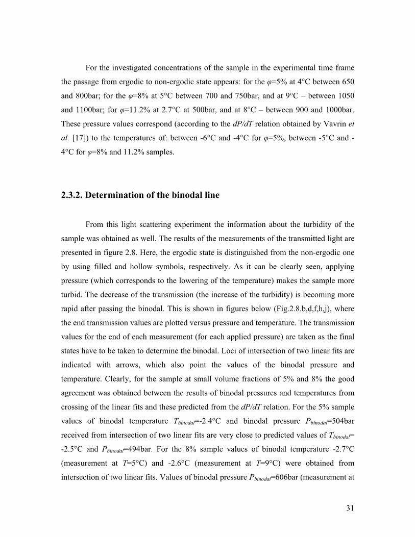
For the investigated concentrations of the sample in the experimental time frame
the passage from ergodic to non-ergodic state appears: for the φ=5% at 4°C between 650
and 800bar; for the φ=8% at 5°C between 700 and 750bar, and at 9°C – between 1050
and 1100bar; for φ=11.2% at 2.7°C at 500bar, and at 8°C – between 900 and 1000bar.
These pressure values correspond (according to the dP/dT relation obtained by Vavrin et
al. [17]) to the temperatures of: between -6°C and -4°C for φ=5%, between -5°C and -
4°C for φ=8% and 11.2% samples.
2.3.2. Determination of the binodal line
From this light scattering experiment the information about the turbidity of the
sample was obtained as well. The results of the measurements of the transmitted light are
presented in figure 2.8. Here, the ergodic state is distinguished from the non-ergodic one
by using filled and hollow symbols, respectively. As it can be clearly seen, applying
pressure (which corresponds to the lowering of the temperature) makes the sample more
turbid. The decrease of the transmission (the increase of the turbidity) is becoming more
rapid after passing the binodal. This is shown in figures below (Fig.2.8.b,d,f,h,j), where
the end transmission values are plotted versus pressure and temperature. The transmission
values for the end of each measurement (for each applied pressure) are taken as the final
states have to be taken to determine the binodal. Loci of intersection of two linear fits are
indicated with arrows, which also point the values of the binodal pressure and
temperature. Clearly, for the sample at small volume fractions of 5% and 8% the good
agreement was obtained between the results of binodal pressures and temperatures from
crossing of the linear fits and these predicted from the dP/dT relation. For the 5% sample
values of binodal temperature Tbinodal=-2.4°C and binodal pressure Pbinodal=504bar
received from intersection of two linear fits are very close to predicted values of Tbinodal=
-2.5°C and Pbinodal=494bar. For the 8% sample values of binodal temperature -2.7°C
(measurement at T=5°C) and -2.6°C (measurement at T=9°C) were obtained from
intersection of two linear fits. Values of binodal pressure Pbinodal=606bar (measurement at

32
T=5°C) and 894bar (measurement at T=9°C) are also very close to predicted values of
581bar and 891bar, respectively. The situation gets slightly worse for the 11.2% sample.
The difference between the values obtained from the intersection of the linear fits and the
values calculated from the dP/dT relation in determination of the binodal temperature is
0.7°C and around 50bar for the binodal pressures. As the same thermometer was used in
all experiments, the possibility of getting bigger error in the temperature determination in
only one case, can be excluded. However, the determination of transdP dT , described by
R. Vavrin et al. [17], gives the values of the binodal temperature with the error of 0.75°C,
so the values obtained from linear fits are still in the agreement with these predicted from
transdP dT within its uncertainty.
0 10 20 30 40 50 600.0
0.1
0.2
0.3
0.4
0.5
0.6
0.7
5min
20min
=5%; T=4degC 1 bar 350 bar 500 bar 650 bar 800 bar 950 bar 1400 bar
Tran
smis
sion
t [min]
0 200 400 600 800 1000 1200 14000.0
0.1
0.2
0.3
0.4
0.5
0.6
0.74 2 0 -2 -4 -6 -8 -10 -12 -14
494bar
= 5% ergodic non-ergodic
Tbinodal = - 2.5oC
for T = 4oC:Pbinodal = 504 bar
P [bar]
-2.4oC
T [ oC]T en
d
(a) (b)
0 5 10 15 20 25 30 35 40
0.1
0.2
0.3
0.4
0.5
0.6
3min6min
10min
13min4min
=8%; T=5degC 1 bar 200 bar 700 bar 400 bar 750 bar 600 bar 800 bar 650 bar 850 bar
Tran
smis
sion
t [min]
0 200 400 600 8000.0
0.1
0.2
0.3
0.4
0.5
0.6
0.0
0.1
0.2
0.3
0.4
0.5
0.6
4 2 0 -2 -4 -6
-2.7oC
606bar
= 8% ergodic non-ergodic
Tbinodal = - 2.5oC
for T = 5oC:Pbinodal = 581bar
T end
P [bar]
T [ oC]
(c) (d)

33
0 10 20 30 40 50 600.0
0.1
0.2
0.3
0.4
0.5
0.6
8min16min
17min
25min
11min3min
=8%; T=9oC 1 bar 400 bar 1000 bar 800 bar 1050 bar 900 bar 1100 bar 950 bar 1200 bar
Tran
smis
sion
t [min]
0 200 400 600 800 1000 12000.0
0.1
0.2
0.3
0.4
0.5
0.6
0.0
0.1
0.2
0.3
0.4
0.5
0.6
8 6 4 2 0 -2 -4 -6
-2.6oC
894bar
= 8% ergodic non-ergodic
Tbinodal = -2.5oC
for T = 9oC:Pbinodal = 891bar
T end
P [bar]
T [ oC]
(e) (f)
0 10 20 30 40 50 60 70 80
0.1
0.2
0.3
0.4
0.5
0.6
0.7
2min
18min
27min
11min
=11.2%; T=2.7oC 1 bar 450 bar 100 bar 500 bar 200 bar 500 bar 300 bar 600 bar 400 bar 1000 bar
Tran
smis
sion
t [min]
0 200 400 600 800 10000.0
0.1
0.2
0.3
0.4
0.5
0.6
0.7
0.0
0.1
0.2
0.3
0.4
0.5
0.6
0.7
2 0 -2 -4 -6 -8 -10
-1.8oC
350bar
= 11.2% ergodic non-ergodic
Tbinodal= - 2.5oC
for T = 2.7oC:Pbinodal = 403bar
T end
P [bar]
T [ oC]
(g) (h)
0 10 20 30 40 50 60 70 80 90 100110120
0.2
0.3
0.4
0.5
0.6
0.7
6min
23min
37min
=11.2%; T=8oC 1 bar 700 bar 200 bar 800 bar 400 bar 900 bar 600 bar 1000 bar
Tran
smis
sion
t [min]
0.1
0.2
0.3
0.4
0.5
0.6
0.7
0.88 6 4 2 0 -2 -4
0 200 400 600 800 1000
0.1
0.2
0.3
0.4
0.5
0.6
0.7
0.8
T [ oC]
-1.8oC
763bar
= 11.2% ergodic non-ergodic
Tbinodal = - 2.5oC
for T = 8oC:Pbinodal = 814bar
T end
P [bar]
(i) (j)
Fig.2.8. Results of the time-dependent transmission measurement for the sample of the volume fraction of:
(a) φ=5% at T=4ºC, (c) φ=8% at T=5ºC, (e) φ=8% at T=9ºC, (g) φ=11.2% at T=2.7ºC, (h) φ=11.2% at
T=8ºC. The filled and hollow symbols stand for the ergodic and non-ergodic state, respectively. The red
lines are the fits done using Eq.2.10. (which is discussed in subchapter 2.3.4.), and the results of the

34
characteristic times are given as well. The end transmission values versus pressure and temperature for the:
(b) 5%, (d) and (f) 8%, (h) and (i) 11.2% sample. The pressure values were calculated to temperature
according to the dP/dT relation. Black lines represent the linear fits, and the loci of their intersections
correspond to the binodal, which is indicated by an arrow. The predicted values of binodal pressures and
temperatures are given.
The time dependency of the transmission, which is presented in figure 2.8.a,c,e,g,i will be
discussed further in subsection 2.3.4.
2.3.3. Analysis of forward scattering intensity and first approach to
determine the spinodal line
In the time-resolved SANS measurements, similarly to the ones done using the
DWS technique, the pressure was applied always from 1bar to the desired value and just
in the moment of reaching it the measurement was started. The difference was the time
interval, which for the neutron scattering experiment had to be higher, due to the lower
intensity of the neutron beam comparing to the light, and it was set to be 5min. Any
process lasting less than 5 minutes would not be resolved because of the low intensity
and wrong averaging reasons.
As an example, there are a few scattering curves for the sample of volume
fraction of 11.2% at T=3°C and at P=500bar plotted in figure 2.9., and in the inset the
magnification of the small q region is given.

35
0.028 0.03 0.032 0.034 0.036 0.038 0.04
500
600
700
800
900
0.1
1
10
100
1000
I(q) /
a.u
.
q [nm-1]
= 11.2%T = 2.7oCP = 500bar
160-165 min 70-75 min 60-65 min 5-10 min 0-5 min
Fig.2.9. The exemplary scattering curves for the sample of the volume fraction φ=11.2% at temperature
T=2.7ºC and pressure P=500bar. Inset: magnification for the small q range.
The shape of the curves remains the same in time after applying pressure, only the
increase in the forward scattering can be observed. It means that the silica particles do not
change their size but they tend to form aggregates. The incompressibility of the silica
particles was proved before by Kohlbrecher et al. [35]. In order to study the time-
dependent development of the forward scattering, the Guinier approximation:
2 2
ln ( ) ln 03gR q
I q I q (Eq.2.9.)
was used. Here, Rg denotes the radius of gyration of a colloidal particle.
The calibration to the absolute scattering intensities could not be done as the
transmission was not measured during the experiment. In the time-slicing experiment it is
not convenient to perform any measurement in between as each transmission
measurement takes a few minutes and it would cause gaps in the time frame of the
experiment. That is why the intensity values had to be corrected for the compressibility of
the solvent (mixture of the hydrogenated and deuterated toluene) with pressure, in other
words: the change of its scattering length density with pressure has to be taken into
account. The relative change in the intensity due to change in the scattering length

36
density of the solvent caused by application of pressure was calculated and the result is
shown in figure below for three different compositions of the solvent, which were used to
prepare the samples.
0 500 1000 1500 2000 2500
1.0
1.2
1.4
1.6
1.8
2.0
2.2
2.4
= 2.6*1010 cm-2
= 2.7*1010 cm-2
= 2.9*1010 cm-2
I(Q=0
,P)/I
(Q=0
,P=1
bar)
P [bar]
Fig.2.10. The relative change in the scattered intensity versus pressure for three different compositions of
hydrogenated and deuterated toluene used in sample preparation.
Obtained from the Guinier analysis (Eq.2.9.) the intensity at q=0 for each concentration
of the sample at each temperature and pressure was then divided by an appropriate factor
(from Fig.2.10.). This way only the change in the scattered intensity coming from the
formation of gel and/or phase separation in the sample will be taken into account and the
contribution of solvent compressibility will be excluded.
Corrected this way intensities at q=0 for different pressures for all samples were
then plotted versus time, which is shown in figure 2.11.

37
0 10 20 30 40 50 60 70
600
800
1000
1200
1400
1600
51 min
=5%; T=2oC 700 bar 600 bar 500 bar 400 bar 300 bar 200 bar 35 bar
I(q=0
) / a
.u.
t [min]
0 10 20 30 40 50 60 70 80
600
700
800
900
1000
1100
1200
1300
1400
=5%; T=5oC 700 bar 600 bar 400 bar 200 bar 35 barI(q
=0) /
a.u
.
t [min]
(a) (b)
0 50 100 150 200400
600
800
1000
1200
14009 min40 min56 min
77 min
1000 bar 600 bar 500 bar 450 bar 400 bar 300 bar 100 bar
I(q=0
) / a
.u.
t [min]
0 20 40 60 80 100 120
400
600
800
1000
120012 min
26 min
1000 bar 900 bar 800 bar 700 bar 600 bar 400 bar 200 bar
I(q=0
) / a
.u.
t [min]
(c) (d)
0 50 100 150 200300
400
500
600
700
800
900
1000
1100
31 min
83 min
8 min12 min
= 16% ; T = 3oC 600 bar 300 bar 500 bar 250 bar 400 bar 200 bar
I(q=0
) / a
.u.
t [min]
0 20 40 60 80 100 120 140 160200
300
400
500
600
700
800
55 min
20 min
= 16%; T = 9oC 850 bar 400 bar 770 bar 300 bar 700 bar 200 bar 500 bar
I(q=0
) / a
.u.
t [min]
(e) (f)
Fig. 2. 11. I(q=0) versus time for the sample: (a) φ=5% at T=2°C; (b) φ=5% at T=5°C; (c) 11.2% at
T=2.7°C; (d) 11.2% at T=8°C; (e) φ=16% at T=3°C; (f) φ=16% at T=9°C. The filled and hollow symbols
stand for the ergodic and non-ergodic state, respectively. The red lines are the fits done using Eq.2.11.
(which will be discussed in subchapter 2.3.4.), the results of the characteristic times are given as well.

38
As it can be clearly seen, applying small pressures does not change the forward
scattering intensity. For example for the 11.2% sample at T=2.7°C the forward intensity
stays constant up to pressure of 300bar and at T=8°C – up to pressure of 600bar (one can
observe a slight increase of its value at P=700bar), see figure 2.11.c and d. Also for the
sample of the volume fraction φ=16% at temperature T=9°C, in figure 2.11.f, no change
in the value of the forward scattering intensity for the applied pressures up to 500bar was
observed. Moreover, in these temperature and pressure conditions all of the samples were
proved by DWS measurement to be ergodic. This indicates that the solution is
homogenous, in other words – it is in the stable (one-phase) region in the phase diagram.
Further application of higher pressures causes an increase in the forward scattering
intensity. This can be observed for the sample of φ=11.2% at T=2.7°C in the pressure
range from 400-600bar, at T=8°C from 800 to 900bar, and for the sample of φ=16% at
T=3°C in the pressure range of 200-400bar. For the 11.2% sample this change is
observed while the solution is still ergodic, whereas for the 16% sample, the increase of
the forward scattering intensity happens when the dispersion turns non-ergodic (it crosses
the percolation line). This increase in the forward scattering would be an indication of the
formation of larger structures (forming clusters or network by the dispersed colloidal
particles). However, for even higher applied pressures, the forward scattering intensity
values level off. This can be seen for example for the 5% sample at T=2°C, where the
intensity values stay constant in the range of around 1300-1500a.u. for pressures of 400-
700bar (Fig.2.11.a), or for the 16% sample at T=3°C, where the intensity values stay
constant in the range of around 1000-1100a.u. for pressures of 500-600bar (Fig.2.11.e).
The system is non-ergodic in these temperature and pressure conditions. This means that
certain structure (the sample volume filling network) was formed and its size will not
change anymore while increasing pressure, at least not in the time-frame of the
experiment. The time-dependency of the forward scattering intensity will be discussed
later on in subsection 2.3.4.
In the figure below, the inverse intensity values are plotted versus pressure and
temperature for the 16% sample. The extrapolation to zero of the time-dependent data,
indicated with black arrows, points the values of the spinodal pressure (and the equivalent
values of temperature according to the dP/dT relation from Vavrin et al. [17]). Here, in

39
figure 2.12.c, the previous results of G. Meier, J. Kohlbrecher, J. Buitenhuis, A. Wilk
from light scattering experiment are also presented.
200 300 400 500 6000.0000
0.0002
0.0004
0.0006
0.0008
0.0010
0.0012
0.0014
0.0016
0.0000
0.0002
0.0004
0.0006
0.0008
0.0010
0.0012
0.0014
0.0016
1 0 -1 -2 -3 -4 -5
=16%; T=3oC non-ergodic
1 / I
end
P [bar]
495bar(- 3.4oC)
T [ oC]
1 / I
end
200 300 400 500 600 700 800 9000.000
0.001
0.002
0.003
0.004
0.005
0.000
0.001
0.002
0.003
0.004
0.0057 6 5 4 3 2 1 0 -1 -2 -3
890bar(- 2.5oC)
=16%; T=9oC ergodic non-ergodic1/
I end
P [bar]
T [ oC]
(a) (b)
0.000
0.001
0.002
0.003
0.004
0.005
0.006
0.0078 6 4 2 0 -2 -4
400 600 800 1000 1200 14000.000
0.001
0.002
0.003
0.004
0.005
0.006
0.007
T [ oC]
1439bar(- 3.5oC)
=16%; T=15.1oC ergodic non-ergodic
1 / I
end
P [bar]
(c)
Fig.2.12. The inverse scattered intensity values versus pressure and temperature for the 16% sample at: (a)
T=3°C; (d) T=9°C; (e) T=15.1°C. The full and hollow symbols stand for ergodic and non-ergodic state,
respectively. The black lines represent the linear fits, and the loci of their extrapolation to zero correspond
to the spinodal, which is indicated by the black arrows; gray lines match the spinodal pressure values with
the spinodal temperatures according to the dP/dT relation from Vavrin et al. [17]. The scattering intensity
in figures (a) and (b) is taken from the SANS experiment, whereas in figure (c) – from light scattering.
As it was already said in subsection 2.1 (see Eq.2.4. and its comment), from the forward
scattering intensity one can obtain the information about the spinodal line. In case of the
16% sample, applying certain pressure (which correspond to lowering temperature to

40
certain value) drives the system first to the percolation. As forming of the network by
colloidal particles takes some time, one has to wait until the structure will be formed,
which will be indicated by leveling off of the scattering intensity (this happens in times
between 30min, after applying P=400bar at T=1.7°C, and 2 hours, after applying
P=200bar at the same temperature). Therefore, the final values of the intensity,
( 0, )I q t , were taken for the 16% sample because then the percolation effects are
assumed to be no longer important. As it can be seen from figure above, the spinodal
occurs at temperature around -3°C for this sample.
In case of the 11.2% sample (and even smaller concentrations), while pressurizing
(lowering temperature), the coexistence line is crossed first; in other words – the phase
separation takes place first. That is why the initial values of the forward scattering
intensity, ( 0, 0)I q t , should be taken to estimate the spinodal. Here, the experimental
limit due to the slicing time of 5 minutes causes problems in analysis of the data. The
access to the forward scattering intensity values at t=0 is possible only through fitting the
I(q=0) vs time data, as it is shown in Fig.2.11. Naturally, then arise the question of the
accuracy of the fit and therefore some doubts about the resulting values appear. The value
of spinodal temperature of around -8°C was obtained this way for the 11.2% sample,
which results in around 6 degrees difference between binodal and spinodal lines. In the
phase diagram of the same system dissolved in benzene obtained by Verduin and Dhont
[27] the difference between binodal and spinodal lines at the same concentration was
only about one degree. That is why the presented here way of determination of the
spinodal temperature (pressure) for 11.2% sample seems to be incorrect due to the
experimental limits.
As it was said in subchapter 2.1 (see Eq.2.5. and its comment), the other way to
determine the position of the spinodal line is introducing the critical scaling law. Here as
well, the initial intensity values, ( 0, 0)I q t , were taken for the sample of φ=11.2%,
and the final values of the intensity, ( 0, )I q t , were taken for the sample of
φ=16%. In figure below, the logarithm of these intensity values is plotted versus
logarithm of reduced pressure, c
c
P P
P
. Here, the critical pressure values, for which

41
the critical exponent is 1 , were found. They are given in the figure below. Obtained
this way values correspond to the results from the linear extrapolation of 1/I(q=0). Again,
the values of spinodal temperature (pressures) for the 11.2% sample obtained from the
scaling procedure can be questioned as the forward intensity values at t=0 are weighted
with considerable uncertainty.
-1.4 -1.2 -1.0 -0.8 -0.6 -0.4 -0.22.3
2.4
2.5
2.6
2.7
2.8
2.9
3.0 495bar
1250bar
800bar
1440bar890bar
=11.2% 2.7oC 8oC
=16% 3oC 9oC 15.1oC
log
I
log
Fig.2.13. Results of the critical scaling law – logarithm of scattered intensity versus reduced pressure
according to Eq.2.5. The values of Pc, for which γ=-1, are given next to the linear fit lines. Again, full and
hollow symbols stand for ergodic and non-ergodic state, respectively.
In table 2.3 the results of the determination of the binodal, spinodal and
percolation lines are summarized. Here, all the pressure values, corresponding to each
transition, were recalculated into temperatures according to the dP/dT relation given by
Vavrin et al. [17]. From the same article, the percolation threshold for the 16% sample
was taken. The values for spinodal obtained in both ways, doing extrapolation and using
the scaling law, are included.

42
Table 2.3. Summary of determination of binodal, spinodal and percolation lines.
binodal percolation φ
[%]
T
[°C] Pbinodal
[bar]
Tbinodal
[°C]
Tbinodal [°C]
from [17]
Ppercolation
[bar]
Tpercolation
[°C]
5 4 494 -2.39 ± 0.01 800 ± 150 -6.32 ± 1.93
5 606 -2.73 ± 0.09 750 ± 50 -4.68 ± 0.65 8
9 894 -2.57 ± 0.05 1100 ± 50 -5.19 ± 0.65
2.7 350 -1.81 ± 0.01 500 -3.75 11.2
8 763 -1.84 ± 0.02 1000 ± 100 -4.90 ± 1.29
16 14 - -
-2.5 ± 0.75
1113 ± 48
from [17] -0.36 ± 0.62
spinodal
extrapolation scaling φ
[%]
T
[°C] Pspinodal [bar] Tspinodal [°C] Pspinodal [bar] Tspinodal [°C]
2.7 798 ± 73 -7.62 ± 0.66 800 -7.6 11.2
8 1249 ± 292 -8.10 ± 1.67 1250 -8.1
3 496 ± 94 -3.40 ± 0.58 495 -3.5
9 889 ± 45 -2.48 ± 1.20 890 -2.55 16
15.1 1439 ± 947 -3.48 ± 1.96 1440 -3.5
In the following chapter the time dependent behaviour of turbidity (transmission)
and forward scattering intensity will be discussed and the spinodal line for low
concentrations will be assumed from it. Then in the discussion, the experimentally
obtained phase diagram of the investigated AHS system will be compared with the
theoretical one.

43
2.3.4. Time dependency and second approach to determine the spinodal
line
Apart from the increase in the turbidity and the forward scattering intensity, the
other feature that appears is the time dependency. In the transmission measurement
evolution with time starts at around the binodal point and can be analyzed with a simple
exponential time behaviour:
0( ) expend end
tT t T T T
. (Eq.2.10.)
Here, 0T and endT denote the transmission values at the beginning and at the end of the
experiment, respectively, and τ is the characteristic time of the decay.
The time evolution of the forward scattering intensity from the SANS experiment, on the
other hand, can be analyzed with:
0( ) 1 expt
I t I A
, (Eq.2.11.)
where I0 is the intensity at t=0, and amplitude is 0endA I I .
In figure 2.14 the values of characteristic time, obtained from using equations 2.10 and
2.11, are plotted versus pressure. The values of binodal and spinodal pressures obtained
from the analysis described in previous subsections (2.3.2 and 2.3.3) are indicated with
gray lines. The differentiation between ergodic and non-ergodic state is again indicated
by using full and hollow symbols, respectively. There was no SANS measurement
performed for 8% sample, and for the 5% sample there were no (or not enough) time-
dependent data to determine the position of the spinodal line. Therefore, in order to mark
possible conditions at which the phase transition to unstable state appears for these two
concentrations, the result obtained for the 11.2% sample was taken. It will then indicate
the highest possible position of the spinodal line in the T(or P-1)-φ plane for these
concentrations, as it is known that the critical point for this system is positioned at
volume fraction higher than 11.2% and the shape of the spinodal line is convex. That is
why the spinodal temperature for concentrations lower than 11.2% cannot be higher than
the spinodal temperature for this concentration. The error bars for the characteristic times

44
are coming from the fitting, and the error bars for temperature and pressure correspond to
the ranges, in which the experiments were held. The temperature in the cell has been
constantly checked while running measurements, and it showed variation of ±0.5°C from
the set temperature. Moreover, the pressure generator was automatically re-pumping the
hydraulic oil into the cell when the actual pressure was more 30bar off from the desired
value.
For the samples of the volume fraction 5%, 8% and 11.2% in the stable state (for
pressures lower than Pbinodal) no time dependency neither in transmission nor in the
forward scattering was observed (see Fig.2.8.a,c,e,g,i and Fig.2.11). Also for the 16%
sample measured at T=9°C, the time dependency of the forward scattering intensity starts
only after applying pressures higher than 500bar. For the same sample investigated at
T=3°C the measurements at pressures lower than 200bar would be needed to see the same
tendency. It can be concluded, that small temperature/pressure changes (after which the
dispersion is still in the stable state) do not cause any time dependent behaviour of the
turbidity and/or forward scattering intensity of the sample. Therefore, data points for
these temperature and pressure conditions will not be given in figures below.
500 600 700 800 900 10000
2
4
6
8
10
12
14
0
2
4
6
8
10
12
14-2 -3 -4 -5 -6 -7
Ps 977bar
(Ts - 7.6oC)Pb =606bar(Tb =
- 2.7oC)
[m
in]
P [bar]
=8%; T=5oC ergodic non-ergodic
T [ oC]
[m
in]
0
5
10
15
20
25
-1 -2 -3 -4 -5 -6 -7 -8
800 900 1000 1100 1200 13000
5
10
15
20
25
T [ oC]
[m
in]
Ps 1287barTs
- 7.6oCPb =894bar(Tb =
- 2.6oC)
[m
in]
P [bar]
=8%; T=9oC ergodic non-ergodic
(a) (b)

45
01020304050607080
0 -2 -4 -6 -8 -10
200 400 600 800 1000
01020304050607080
T [ oC]
[m
in]
=11.2%; T=2.7oCSANS: ergodic non-ergodicTrans.: ergodic non-ergodic
Ps = 798bar
(Ts = - 7.6oC)
Pb =350bar(Tb =
- 1.8oC)
[m
in]
P [bar]
0
5
10
15
20
25
30
35
0 -1 -2 -3 -4 -5 -6 -7 -8
600 700 800 900 1000 1100 1200 13000
5
10
15
20
25
30
35
T [ oC]
[m
in]
Ps =1250bar(Ts =
- 8.1oC)
Pb =763bar(Tb =
- 1.8oC)
[m
in]
P [bar]
=11.2%; T=8oCSANS: ergodic non-ergodicTrans.: ergodic non-ergodic
(c) (d)
0
20
40
60
80
1000 -1 -2 -3 -4 -5
200 300 400 500 600
0102030405060708090
100
T [ oC]
[m
in]
Ps = 495bar
(Ts = - 3.4oC)
= 16%; T = 3oC non-ergodic
[m
in]
P [bar]
600 700 800 900
0
10
20
30
40
50
60
70
0
10
20
30
40
50
60
701.0 0.5 0.0 -0.5 -1.0 -1.5 -2.0 -2.5
Ps = 890bar
(Ts = - 2.5oC)
[m
in]
P [bar]
= 16%; T = 9oC non-ergodic
T [ oC]
[m
in]
(e) (f)
Fig. 2.14. Characteristic times versus pressure for: (a) φ=8% at T=5ºC, (b) φ=8% at T=9ºC, (c) φ=11.2% at
T=2.7ºC, (d) φ=11.2% at T=8ºC, (e) φ=16% at T=3ºC, (f) φ=16% at T=9ºC. The characteristic times for 8%
sample come from transmission measurement, for 16% sample – from SANS measurement, and for 11.2%
sample – from both techniques. As before, ergodic state is marked with full symbols and non-ergodic with
hollow symbols. Additionally, values of binodal and spinodal pressures are indicated with gray lines.
The most detailed measurement was carried for the 8% sample (Fig.2.14.a and b).
Here, it is clearly seen that the time dependency starts after passing the binodal line, at
the beginning the characteristic time is small – system reaches the equilibrium state fast,
then it increases (it takes longer for the system to equilibrate) until the transition to the
non-ergodic state appears and after passing the percolation line one can observe the
tendency: the deeper the quench is, the faster it gets for the system to reach its final state.

46
For the sample of volume fraction of 11.2%, which is shown in Fig.2.14.c and d,
after the pressure jump of around binodal pressure value, the time evolution started as in
the case of 8%. However, for this sample, and especially in the measurement taken at
T=8°C (Fig.2.14.d), one can observe the tendency that the higher the pressure was
applied, the faster system reaches its final state even before passing percolation line,
unlike for the 8% sample. But, naturally, one can claim that a measurement for pressure
between 700 and 800bar would be needed to state firmly if that is actually the case or if,
simply, the additional measurement would reveal the same tendency observed for the 8%
sample. Especially, that the transmission results for the 11.2% sample measured at
T=2.7°C show the similar tendency as the sample of φ=8%.
It is even more difficult to make any statement about the 5% sample as there are
not enough results. Although here, one can observe that after applying very high
pressures (from 950 to 1400bar), the system is brought immediately to its final state – no
time-dependency is observed anymore (see Fig.2.8.a and b).
For the 16% sample the situation is different. Here, the time dependency starts
after passing the percolation line and it shows the tendency that the bigger the quench
(pressure jump) is, the shorter time is needed for the sample to reach its final state. After
passing the spinodal line, no time-dependency is observed any more.
As it was said in the previous subchapter, the values of spinodal temperature
(pressures) for the 11.2% sample obtained from the extrapolation of inverse forward
scattering intensities at t=0 and from the scaling procedure are weighted with
considerable uncertainty. That is why other approach to determine the spinodal line is
proposed. Bringing the system by quenching (changing temperature and/or applying
pressure) into unstable state, the phase separation will proceed through the spinodal
decomposition mechanism. In this case any (even small amplitude) density fluctuations
decrease the Helmholtz free energy and lead to decomposition. Performing deeper
quench into the unstable state will cause larger inhomogeneities and the demixed state
will be reached faster, which one can attribute to the decrease in characteristic time τ.
Therefore, at these temperature and pressure conditions, where τ decreases, the transition
to the unstable state (passing spinodal line) can be expected. The pressure values, at
which the maximum in characteristic time was observed, are summed up in table 2.4.

47
Table 2.4. Summary of the spinodal line determination from the characteristic times of transmission and
forward scattering intensity time dependency.
φ [%] T [°C] Pspinodal [bar] Tspinodal [°C]
5 4 650 ± 150 -4.39 ± 1.93
5 700 ± 50 -4.03 ± 0.64 8
9 1150 ± 50 -5.84 ± 0.64
2.7 450 ± 100 -3.11 ± 1.29 11.2
8 800 ± 100 -2.32 ± 1.29
The values of spinodal temperatures for each concentration given in the last column in
the table above were calculated using dP/dT relation.
2.4. Discussion
Finally, in figure 2.15 the experimentally obtained binodal, spinodal and
percolation lines are plotted on the theoretical phase diagram. The positions of the
spinodal line from both approaches, from analysis of forward scattering intensity
(extrapolation and scaling) and from maximum in characteristic times, are marked with
solid and dashed blue lines, respectively. The experimental results concerning the
position of the percolation threshold for samples of volume fractions 1% and 39.2% and
binodal line for 1% sample from Vavrin et al. [17] are added in the figure. The stickiness
parameter, in which the theoretical phase diagram calculated by Miller and Frenkel [16]
and by Fantoni et al. [26] (C1 model) was expressed, was re-calculated into temperature
in Celsius scale using:
0 27312
ln2
B
LT
LR
. (Eq.2.12.)

48
The radius of the colloidal particles were determined as R=34.2nm by Kohlbrecher et al.
[35], and the values of Δ=0.5nm, 0 =282K and L=107 were taken from Vavrin et al.
[17].
0.0 0.1 0.2 0.3 0.4
-8
-6
-4
-2
0
2T
[ o C]
volume fraction,
percolation binodal
spinodal Miller & Frenkel C1 model
Fig.2.15. The phase diagram of AHS system – comparison of theory with experimental results.
Depending on the location of the spinodal line for low concentrations, two possible
scenarios can be given. The first one will describe the situation, where the spinodal line
(determined from the analysis of the forward scattering intensity) lies much lower than
the coexistence line. In this case phase separation will be realized via nucleation
mechanism. The second scenario relates to the situation, where the spinodal line
(determined from the maximum in the characteristic time) is placed close to the binodal
line and the phase separation by spinodal decomposition mechanism is possible.
Regardless the method of determining the spinodal line for low concentrations, the results
for 16% sample can be easily explained, as its behaviour is grossly affected by
percolation effects and this case will be discussed firstly. Then both of the scenarios of
phase behaviour for lower concentrations will be given.

49
2.4.1. Phase behaviour of 16% sample
What differs the sample of volume fraction φ=16% from those of lower volume
fractions, is that here while pressurizing (lowering temperature), the transition from
ergodic to non-ergodic state is observed first. Only after decreasing temperature even
more, the phase separation starts. The position of percolation threshold was already
determined by Vavrin et al. [17] for the measurement done at T=14°C. The non-ergodic
behaviour appeared after applying pressure of 1113bar, which corresponds to lowering
temperature to: 1113
14 0.477.5perc
barT C C . It can be also seen from the SANS data
taken at T=9°C that applying pressures lower than 700bar (which corresponds to
lowering temperature to around 0°C) does not cause any transition – the dispersion stays
in the stable state (see Fig.2.11.f). This is reflected in the lack of the time dependency of
the forward scattering intensity. For higher pressures, in other words – for lower
temperatures, the system percolates. This is reflected not only in the increase of the
forward scattering intensity but also in its evolution with time. Formation of a percolating
network is a process that takes some time, moreover, one can see the tendency that the
deeper the quench is (the higher the pressure jump amplitude), the faster it takes for the
system to reach its final state. The final state is reflected by a time-independent forward
scattering intensity value. The systems gels faster because the interactions are stronger,
the stickiness parameter gets smaller. At some point, after lowering temperature
significantly enough (for example by applying pressure of 850bar, which corresponds to:
8509 2
77.5
barT C C ), system reaches its final state immediately. This, on the other
hand, is the location of the coexistence line, which is known from the theoretically
predicted phase diagram (see Fig.2.15). Moreover, for the sample of this volume fraction,
the spinodal line is expected to be located near the binodal line – around one degree
lower, which is in the range of the experimental uncertainty. The fact that the intensity is
becoming time-independent at large pressure amplitudes means simply that here a so
called gelation assisted by phase separation is taking place. This mechanism was already
proposed by Verduin and Dhont [27] and by Verhaegh et al. [15]. To sum up, the

50
increase of the forward scattering intensity for higher pressures is governed by the
proximity to the spinodal line but the percolation effect controls the time scale. The
growth of the scattering intensity is due to the evolution of a critical structure which was
proved to follow a mean field type of scattering behaviour [17].
2.4.2. First scenario of phase behaviour of low concentrated samples –
phase separation through nucleation process
The transient behaviour for the 5% and 8% samples can be seen in the results of
the light transmission measurement, see figure 2.8.a,c,e. The experimentally obtained
temperature and pressure conditions at which binodal line appears are in the agreement
with the previous predictions of Vavrin et al. [17] (see Fig.2.8.b,d,f). Also the position of
the percolation line was determined from the DWS experiment.
On the other hand, the SANS data for the 5% sample are the only ones
characterized by the difficulty to observe time dependency. The only trace of it appears at
T=2°C and P=300bar, see figure 2.11.a. The increase of the forward scattering intensity
can be observed between 300bar and 400bar in the measurement done at T=2°C, and
between 400 and 600bar in the measurement done at T=5°C. In these temperature and
pressure ranges the transition from a stable into a two-phase state is expected, as –
according to dP/dT relation and binodal temperature obtained previously by Vavrin et al.
[17] – at T=2°C the pressure value of around (2 2.5) 77.5 350binodalP bar should be
applied to reach the phase separation, and at T=5°C: (5 2.5) 77.5 580binodalP bar .
Inspecting figure 2.11.a and b more closely one also notices no further increase of I(q=0)
with pressure, from 400bar to 700bar at T=2°C, where the scattered intensity stays in the
range of 1300-1500a.u. (see Fig.2.11.a), and from 600bar to 700bar at T=5°C, where it
stays in the range of 1200-1400a.u. (see Fig.2.11.b). In the SANS experiment, the 5%
sample was brought from the stable state (T=2°C, ambient pressure) to percolated state
by applying pressure of 700bar, which correspond to lowering temperature of about 9°C.
In the light of the results of the spinodal temperature determination from analysis of

51
I(q=0) for other concentrations, the 5% sample at temperature of around 7T C is
expected to be in the meta-stable region in the phase diagram, therefore it is expected to
decompose via nucleation process. However, due to the presence of the percolation line
(that appears possibly even at around -3°C or -4°C), the demixing process is restricted by
the percolation effect. The colloid-rich phase is characterized by a percolated state giving
rise to a non-ergodic scattering behaviour.
In the DWS and turbidity measurements this sample was brought, by applying
pressure of 1400bar, from stable state at T=4°C and ambient pressure to (probably)
unstable state at 14T °C. The time dependence of the transmitted light can be still
seen at P=800bar (which correspond to 6T C ), where the system is already non-
ergodic but not yet unstable. It vanishes at around P=950bar (which correspond to
8T C ). Any change in the transmission was not observed for pressures 950-1400bar,
at least not within the accuracy of the photodiode used in the experiment. In the meta-
stable region the time dependency of transmitted light can be observed, which can be
explained with increasing turbidity of the sample whilst formation and growth of the
droplets of the colloid-rich phase. On the other hand, no time dependency in the forward
scattering intensity could come from the fact that the position of the spinodal is at much
lower temperatures, and in the investigated temperature and pressure range the system is
far away from this transition.
At the volume fraction of 8%, as for the 5% sample, the binodal is crossed first
upon pressurizing, after which the time dependency of the transmitted light starts. This
transient behaviour has a distinct maximum in the characteristic time τ, which was
derived from equation 2.11, and it is shown in figure 2.15.a and b. At the beginning,
characteristic times exhibit increasing tendency with pressure until a point, where the
percolation effects come into play, and then they decrease. For phase separation many
processes over a variety of time- and length-scales are involved, like initial structure
formation, mass transport via diffusion and droplet coalescence. Therefore, the point at
which time dependence sets in is associated with location of the phase separation. Initial
increase in characteristic time while applying higher pressures reflects the fact that higher
density gradients build up and the system needs longer time to reach its equilibrium state.
This slow evolution of the turbidity takes place in the pressure range of 650-750bar at

52
T=5°C, and 900-1050bar at T=9°C. But this trend is abruptly broken at somewhat higher
pressures for both temperatures. Specifically, the system becomes non-ergodic as
deduced from DWS measurements just after maximum in τ was reached. In other words,
phase separation via nucleation and growth is a fully ergodic process. But when the
percolation transition is crossed, the higher pressure is applied, the faster it takes for the
system to reach its final state. Eventually, for high enough pressures the system gels
immediately. One has to keep in mind that each time the pressure quench (which
correspond linearly to lowering temperature) was done from ambient to the desired value
within seconds up to a few minutes, depending on the depth of the quench, which means
that the system was driven very fast from the stable to the biphasic or percolated state.
To sum up, for these both low concentrations the percolation line was observed at
lower temperatures than the coexistence line, the difference is roughly about 2°C. The
location of the percolation line below the binodal line is in agreement with previous
theoretical and experimental findings [11,[13,[14,[27]. The phase separation already
starts in a temperature range, where no percolation was observed, and its kinetics changes
as soon as the percolation line is crossed. The spinodal line lies below the percolation line
and the unstable state of the system is characterized by vanishing of time dependency in
turbidity of the sample.
The 11.2% sample was characterized using SANS and DWS combined with
turbidity measurements. In this case, for both, forward scattering intensity and
transmitted light, the time dependency could be observed. The temperature and pressure
conditions at which binodal line appears, obtained from the turbidity measurement, are in
the agreement with the predictions of Vavrin et al. [17] within the uncertainty coming
from the dP/dT relation (see Fig.2.8.h and j). The results of the DWS experiment for this
particular concentration are especially interesting because they reveal that the percolation
effect sets in some time (around 1 hour in this case) after applying pressure (see Fig.2.11c
for 500bar). On this basis one can expect to observe similar behaviour for the lower
pressure values (400bar and 450bar at T=2.7°C) after times longer than the time-frame of
the experiment. Both DWS measurements, at T=2.7°C and at T=8°C, give the percolation
threshold for this concentration at temperature of around -4°C (within the experimental

53
error), which is about 1.5 degrees lower than the binodal line. The position of spinodal
was determined from the analysis of the forward scattering intensity from SANS
experiment: on one hand from extrapolation of the inverse intensity versus pressure
(temperature), and on the other – using critical scaling law. Both approaches gave similar
result and the transition to unstable state is expected to appear at around -8°C, which is 4
degrees lower than the percolation threshold. The sample stays stable when pressures up
to 300bar at T=2.7°C and pressures up to 700bar at T=8°C are applied. This corresponds
to lowering temperature to around -1°C, where the system is still in the stable state. The
time dependent behaviour of the turbidity of the sample as well as the of time dependent
behaviour the forward scattering starts after passing the coexistence (binodal) line (see
Fig.2.15c and d). The passage from stable to biphasic region appears at temperature of
around -2°C. In principle the tendency: the bigger pressure applied, the faster it gets for
the system to reach its final state, is observed. At temperature of around -4°C the
transition from ergodic to non-ergodic appears, and bringing the dispersion into even
lower temperatures (pressurizing more) causes vanishing of time dependency. The
percolation is immediate. Then, at temperature of around -8°C the transition to unstable
state is expected.
To conclude, this scenario of phase behaviour of the investigated AHS system
explains why time dependency in I(q=0) in SANS experiment for very low concentration
(5%) was not observed. It is due to the location of the spinodal at much lower
temperatures, and in the investigated temperature and pressure range the system is far
away from this transition. Thus, phase separation for low concentrations of the sample
proceeds through nucleation mechanism, which is a fully ergodic process. However, such
temperature difference between the position of binodal and spinodal lines is rather
unexpected. This rather big difference shows discrepancy with the findings of Verduin
and Dhont [27] for the same AHS system consisting of silica spheres grafted with stearyl
alcohol dispersed in benzene (which, as well as toluene, is a marginal solvent for the
octadecyl chains). There, the spinodal lies of around 2 degrees lower than the coexistence
line at volume fraction of 5% and around 1 degree at 10%. The gel line found in this
work was obtained using DLS and visual observation of the scattered speckle pattern and
54
pertains to static percolation, whereas the theoretical predictions give presumably
dynamic percolation, i.e. a case of an infinite cluster at each instant of time with
configuration changing in time. Using DWS technique determine rather the dynamic
percolation threshold, therefore presented here results are in agreement with theoretical
phase diagram, unlike Verduin and Dhont findings [27].
2.4.3. Second scenario of phase behaviour of low concentrated samples –
phase separation through spinodal decomposition process
This case differs from the previously described in the way of determination and
thus the location of the spinodal line. As it was proposed in chapter 2.3.4, passing of the
system into unstable state is attributed to the maximum in the characteristic times of
turbidity and forward scattering intensity time dependency. The location of coexistence
and percolation lines stays the same as in the first scenario.
Here, the phase separation takes place mainly through spinodal decomposition
process, as the spinodal lies closer to binodal line than in the previous case. For the 8%
sample the gap between coexistence and spinodal line is of around 100bar (which
corresponds to 1.3 degrees) for the measurement taken at T=5°C, and of around 150bar
(1.9 degrees) for the measurement at T=9°C. For the 11.2% sample this gap is of about
50bar (which corresponds to 0.6 degrees) for the measurement taken at T=2.7°C, and
about 100bar (1.3 degrees) for the measurement at T=8°C. These results follows the
expected tendency that while lowering concentration, the distance between coexistence
and binodal line should increase, as for the volume fractions below the critical point the
shape of the spinodal line is convex. Obtaining relatively small temperature difference
between coexistence and spinodal lines (comparing to the estimation given in the first
scenario) is in agreement with the findings of Verduin and Dhont [27] for the same
system dissolved in benzene. Taking results for 8% sample, in this gap the time-
dependent increase of turbidity (equivalent to the decrease of transmission) goes slower
after applying higher pressure, see Fig.2.14.a,b. This can be attributed to the formation of
droplets, as in this small temperature range phase transition would be realized through

55
nucleation mechanism. After crossing the spinodal line, a decrease in characteristic time
can be observed. Within this process percolation sets in, which can be seen especially in
the results of turbidity measurement for 11.2% sample at T=2.7°C, where around one
hour after applying pressure of 500bar the system becomes non-ergodic. Eventually after
applying sufficiently high pressures, the final state is achieved immediately by the system
(time dependency neither in turbidity not in forward scattering intensity is observed any
longer). In this scenario, the percolation appears immediately (within additional 50bar,
which corresponds to 0.6 degrees) after transition to unstable state for 8% sample. For
11.2% sample the gap between these two is of around 100bar (1.3 degrees) for the
measurement at T=2.7°C, and about 200bar (which corresponds to 2.6 degrees) at T=8°C.
Inspecting experimental phase diagram presented in Fig.2.15, one can see that the
difference between percolation and spinodal line is within the error bar. This is in
agreement with findings of Lu et al. [29], which says that not only demixing proceeds
through the spinodal decomposition, but also it initiates the gelation of particles, which is
a direct consequence of equilibrium liquid-gas phase separation. The formation of density
fluctuations, caused by thermodynamic instability (spinodal decomposition), leads to
spanning clusters that dynamically arrest to form a gel. The authors also claim that it is
independent from microscopic system, and should be applied to any particle system with
short-range attractions.
2.5. Conclusions
The transition of the investigated AHS system to the percolated state was
unambiguously determined using the double-cell DWS technique and the results are in
agreement with the theoretical predictions. Also the position of the coexistence (binodal)
line, obtained from the transmission (turbidity) measurement, corresponds to the one
given theoretically. Two approaches of spinodal line determination were proposed for the
low concentrated (5%-11.2%) samples: one based on analysis of the forward scattering
intensity and later related to time-dependent behaviour of the turbidity and the forward
scattering of the sample. For the high concentrated sample (16%), only the first approach

56
was used to assign the transition to unstable state. The first method gives the difference of
around 6 degrees between binodal and spinodal temperatures for the 11.2% sample (see
blue solid line in Fig.2.15). For lower concentrations it is expected to be even bigger.
Moreover, in this scenario the spinodal line lies below the percolation line, which means
that the gelation occurs before the phase separation takes place. The other approach
results in much smaller difference between binodal and spinodal temperatures in the
investigated concentration range (up to around 2 degrees, see blue dotted line in
Fig.2.15), and in this case the spinodal line lies above the percolation line, which means
that gelation is preceded by the spinodal decomposition process. At this point, it is hard
to judge which one (or if any of them) is correct. Nevertheless, from the results for 11.2%
sample one can see that transition from ergodic to non-ergodic state sets in when the
system is phase separating and moreover, it can happen after some time after quenching
(see Fig.2.7.b). This means that the difference between phase separation and percolation
can be distinguished. For 16% sample the observed increase of the forward scattering
intensity for higher pressures is governed by the proximity to the spinodal line and it is
due to the evolution of a critical structure which was proved to follow a mean field type
of scattering behaviour [17]. The percolation effect controls the time scale of the increase
of the forward scattering intensity.
In order to solve the problem of determination of spinodal line the small angle
light scattering measurement could be performed, as it has advantage over SANS
technique because it gives access to smaller q-range and, due to the higher flux, the
shorter measurements can be taken, which gives more detailed information about kinetics
of the processes that the system undergoes. However, the difficulty that has to be solved
first is the turbidity of the sample, which spoils the classical light scattering experiments.
The pressure cell for SALS is similar to the one used in SANS experiments [39] and the
sample is placed in a pill of 2mm thickness. The preliminary attempts were already made
to diminish the optical path length through reducing the sample thickness to 1mm by
using glass window with thickening in its centre but this turned out not to be sufficient.

57
3. Temperature- and pressure-dependent behaviour of PEP-PEO
polymeric micelles in water and water-DMF solutions
3.1. Introduction
The study of the deformation and phase behaviour of soft particles, such as
proteins, (micro)gels or polymers, induced by pressure has attracted a lot of interest not
only for the understanding of mechanisms that govern the phenomenon but also because
of the whole range of technical applications. For example, some bacteria can live under
extremely high pressure and low temperatures in the deep ocean [44], therefore study of
behaviour of proteins under pressure is of biological relevance, as proteins structure and
dynamics determine their biological functions [45-[48]. Also polymers are used under
high pressure: in lubrication, where fluid pressure can reach values up to 40kbar [49], or
as viscosifiers to enhanced oil recovery fluids, where pressures of a few thousand
atmospheres are encountered [50], to mention only a few examples of industrial
application. Moreover, pressure as an experimental variable has a twofold advantage.
Changing of pressure can be performed much faster than varying of temperature. Also
using temperature jumps one has to wait longer until the whole sample will be equally
heated or cooled down.
Among other polymers, poly(ethylene oxide) (PEO) has attracted a lot of interest.
Due to its unique properties [51-[60], it has been extensively studied for understanding
the behaviour of polymer solutions and also for its broad range of technical applications
[61-[63]. It readily adsorbs at particle interfaces [64], confers steric stability [65,[66], acts
as good retention aid, surfactant and drag reducing agent in industrial process [67-[69]. It
has been investigated as well as for its biological applications [70], as it is biocompatible
and inhibits protein adsorption [71,[72]. Unlike its lower and higher homologues, PEO is
soluble not only in large number of organic solvents but also in water up to around
100ºC. The solubility of PEO is due to hydrogen bonding between the oxygen on the
polymer chain and the water molecules. An increase in temperature causes the reduction
of hydrogen bonds, which decreases the solvent quality and leads to phase separation.
There is much experimental [51-[57] and theoretical [58-[60] research on the phase

58
behavior of PEO/water systems, also concerning pressure dependence. PEO in water
exhibits a lower critical solution temperature (LCST), above which there is a two-phase
region. Cook et al. [55] showed, in addition, that application pressure of around 4kbar
dramatically lowers the LCST of PEO in water to room temperature. On the other hand,
also below room temperature the solvent quality is reduced and the pressure required to
induce a phase separation can be lower. The worsening of the solvent quality below room
temperature may be due to the van der Waals attraction between them or the formation of
the water tetrahedral network with less liable hydrogen bonds, which frustrates the fit
between PEO and the water network [59].
Even more interesting systems are polymeric micelles due to their more complex
structure. Block copolymers poly(ethylene-co-propylene-b-(ethylene oxide)) (PEP-PEO)
form micelles in water, as PEP is hydrophobic and forms a compact core surrounded by a
shell of hydrophilic PEO. Self-assembling into well defined micelle with segregated core-
shell structure is attributed to the high incompatibility of PEP and water which results in
a large interfacial tension between the two components [73]. Moreover, from the high
incompatibility of PEP with PEO a sharp core-shell interface is expected [74]. Phase
behaviour of these block copolymer micelles in water will depend on PEO solubility,
especially in the case of highly asymmetric structure, where PEO chains are much longer
than PEP. Therefore phase separation of PEP-PEO micelles and PEO is expected at the
same temperature and pressure conditions.
Another way to tune the solvent quality for PEP-PEO micelles is addition of
DMF. It results in a significant decrease of the interfacial tension between PEP and the
solvent (from γ=46mN/m in pure water to γ=8.6mN/m in pure DMF [73]), which entails
reduction of the aggregation number as compared to that in pure water. It was found for
highly asymmetric micelles PEP1-PEO20 (where numbers stand for the approximated
molecular weight in kg/mol) that in the extreme case of dissolving these block-
copolymers in pure DMF only unimers exist [73]. On the other hand, addition of DMF
reduces the solvent quality for PEO, which leads to shrinkage of the micellar corona [73].
Influence of DMF on both, PEP and PEO, causes formation of smaller micelles than in
pure water both, in terms of aggregation number and corona diameter. Moreover, it was

59
found that for polymers in good solvents the radius of gyration shows no consistent trend
with pressure since it may either increase or decrease with increasing pressure [75].
The pressure-dependent behaviour of polymers, gels and surfactants has attracted
a lot of interest. Also behaviour of proteins (especially casein) under pressure has been
investigated extensively due to its applications in food processing [76]. However, the
effect of pressure on polymeric micelles was not extensively investigated so far [77,[78].
Therefore the aim of the present work was to study the influence of pressure on micellar
system, as a model example of a simple structural soft matter system, represented in our
case by the PEP-PEO diblock copolymer dissolved in water and in water-DMF mixture.
This is the first pressure-dependent experiment on this particular micellar system. For
each solvent there is a different scenario of what is happening with the system under
action of pressure: in water solution a size (radius of gyration) change can be observed
and in water-DMF solution – a phase separation induced by pressure. Both scenarios are
sketched schematically in Fig.3.1.
(a)

60
(b)
Fig.3.1. Schematic representation of the concept of the experiment: (a) investigation of pressure influence
on the size of the PEP-PEO micelles in water solution, (b) investigation of phase separation induced by
pressure.
These two solvents were chosen because of the difference in the quality for PEO
and because of the change in the interfacial tension between PEP and the solvent, as
described above. Therefore bigger micelles are expected to be formed in water than in
water-DMF solution. Here, we would like to compare the influence of pressure on the
same copolymer, which in different solvents will self-assemble into micelles of different
sizes. In the case of PEP-PEO micelles in water, the measurements were taken in such a
temperature and pressure range that the system was always in the single-phase region, as
we wanted to study the influence of pressure on the micellar radius of gyration. The
importance of this experiment comes from the need to determine the form factor from the
single particle study before going into more complex case of more concentrated solution
and also to study later phase kinetics of soft spheres. On the other hand, for the same
system in water-DMF solution a macroscopic phase separation induced by pressure could
be observed. The goal is to probe the phase transition induced by pressure (temperature
and pressure conditions at which it appears, its reversibility). This system is more
susceptible for changes in the environment than water dispersion because DMF is worse
solvent for PEO than water. The highly asymmetric block copolymer was chosen because

61
it was expected to see more pronounced reply to change of temperature and pressure than
the micelles with much smaller corona.
This chapter is organized as follows: experimental section consists of two
subunits describing materials, where information about the properties of both solvents as
a function of temperature and pressure is described, and experimental techniques and
setups, where the description of light scattering techniques and theory about fitting
functions used in the analysis of SANS data is given. Results are presented in subchapters
3.3. and 3.4., which are subdivided, according to the investigated system and used
technique. This is followed by the discussion and all is concluded in the last subchapter.
3.2. Experimental section
3.2.1. Materials
The poly(ethylene-propylene)-poly(ethylene oxide) diblock copolymer dhPEP5-
hPEO120 and the homopolymer poly(ethylene oxide) hPEO150, provided by Jürgen
Allgaier, was used. Here, the letters d and h stand for deuterated and protonated,
respectively, and numbers denote approximated molecular weight in kg/mol. The details
of the synthesis procedure as well as the characterization of the diblock copolymer were
published elsewhere [79]. The gel permeation chromatography (GPC) measurement
revealed the molecular weight Mw=117995g/mol and the polydispersity index PD=1.06
for the block copolymer dhPEP5-hPEO120, and Mw=129686g/mol and PD=1.05 for the
homopolymer hPEO150. Two solutions of the diblock copolymer were prepared: one in
D2O and the other one in the mixture of D2O-dDMF of mole fraction dDMFx =0.5, both at
a volume fraction of Φ=0.33%. Also a solution of the hPEO150 homopolymer in the
mixture of D2O-dDMF was prepared, where dDMFx was also 0.5, at a concentration of
c=2.64mg/ml (which corresponds to volume fraction of Φ=0.23%). The concentration
was chosen to be around half of the overlap concentration, c*. Using the expression for
the radius of gyration for PEO in water proposed by Devanand and Selser [80]:

62
0.583 0.0310.215g wR M Å, the overlap concentration estimated from 34*
3w
gA
Mc R
N
gives c*=5.89mg/ml.
As the homopolymer and block copolymer are fully or partially protonated, the
deuterated solvents were used in order to obtain a good contrast in the SANS experiment.
The same mixtures were measured also with light scattering techniques. The parameters
concerning molecular weights, densities and scattering length densities of used polymers
presented in the table below were taken from the PhD thesis of Andreas Poppe [81].
Table 3.1. Properties of the dhPEP5-hPEO120 diblock copolymer.
molecular weight of the copolymer M g mol 128000±6500
(GPC – 117995)
molecular weight of the brush polymer
(hPEO120) MhPEO120 g mol 123060±6200
molecular weight of the core polymer
(dhPEP5) MdhPEP5 g mol 4940±250
molecular weight of the PEO monomer MPEO g mol 44.0
molecular weight of the PEP monomer MPEP g mol 75.8
density of PEO (at ambient conditions) dPEO 3/g cm 1.125
density of PEP (at ambient conditions) dPEP 3/g cm 0.924
volume of the brush polymer (hPEO120) VhPEO120 3Å 8877.98
volume of the core polymer (dhPEP5) VdhPEP5 3Å 181645.08
density of copolymer (at ambient
conditions) d 3/g cm 1.1156
scattering length density of the brush
polymer (hPEO120) hPEO 2cm 96.37 10
scattering length density of the core
polymer (dhPEP5) dhPEP 2cm 104.1 10
volume fraction Φ - 0.0033

63
Table 3.2. Properties of the homopolymer hPEO150.
molecular weight M g mol 129686
density (at ambient conditions) d 3g cm 1.125
scattering length density of the polymer
(hPEO150k) hPEO 2cm 96.37 10
scattering length density of the solvent
(dDMF/D2O) 2/dDMF D O 2cm 106.33756 10
concentration c g ml 32.64 10
D2O (Aldrich, Deuterium oxide 99.9% D) and DMF-d7 (Chemotrade, Leipzig,
Germany, N,N-Dimethylformamid-d7 99.5% D; further called dDMF) for the DLS
measurements were purified using the 0.2μm filters. For the SANS experiment no further
purification was performed. The characterization of both solvents is given in table 3.3.
Table 3.3. Solvents – parameters.
molecular weight of D2O MD2O g mol 20.04
molecular weight of
dDMF MdDMF g mol 80.15
bound coherent scattering
length of 2H bc [fm] 6.671
bound coherent scattering
length of 16O bc [fm] 5.803
bound coherent scattering
length of 12C bc [fm] 6.6511
bound coherent scattering
length of 14N bc [fm] 9.37
In order to analyze the data from DLS and SANS experiments properly, it is
important to estimate how the density (d), refractive index (n), viscosity (η) and

64
scattering length density (ρ) of the solvents are varying with changing temperature and
pressure. Pressure dependence of refractive index can be determined using the Lorentz-
Lorenz equation (which is an extension of the Claussius-Mossotti equation to the region
of optical frequencies): 2
2
1 4
2 3 w A
nd
n M N
, where α is the electric polarizability, as it is
discussed by Vedam and Limsuwan [82]. The pressure-dependent values of the refractive
index at given temperature are then easily calculated (knowing the density in function of
temperature and pressure, and the refractive index as a function of temperature) from the
ratio:
2
2
( ) 1 2 ( ) 1 (1 )
(1 ) 1 2 (1 ) 1 ( )
n P Cd P Cd bar
n bar Cd bar Cd P
, (Eq.3.1.)
where the constant C is given by 2
2
1 (1 ) 1
(1 ) (1 ) 2
n barC
d bar n bar
, as it is described elsewhere
[83].
From the temperature and pressure dependent values of density, the scattering length
density can be calculated using the formula:
1( , )( , )
i
n
ci
m
bT P
V T P
, (Eq.3.2.)
where: icb is the bound coherent scattering length of ith of n atoms in a molecule,
( )( , )m
A
MV P
d T P N
– molecular volume at certain temperature T and pressure P.
The density and the refractive index of both solvents, D2O and the equi-molar
mixture of D2O-dDMF, in the temperature range of interest and at ambient pressure were
measured with an oscillation U-tube density meter (Anton Paar, DMA 4500 Density
Meter) and refractometer (Abbemat® RXA 156).
Pressure-dependent values of density of D2O were taken from the literature [84,[85]. The
values of density of D2O from Emmet et al. [84] were given only for the temperature
range of 2-40ºC and the pressure range of 0-1000bar. In order to expand the pressure
range up to 2500bar for the temperatures T=9ºC and T=20ºC, the 2nd polynomial fit

65
d(P)=A+B1·P+B2·P2 was performed. The pressure-dependent density values at
temperatures of T=50ºC and T=70ºC were taken from Lee and Jonas [85] and could be
fitted also using 2nd polynomial fit. The resulting values of the coefficients from 2nd
polynomial fits for each temperature are given in table 3.4.
Table 3.4. Coefficients from 2nd polynomial fit of pressure-dependent D2O density: d(P)=A+B1·P+B2·P2
for temperatures: 9, 20, 50 and 70ºC.
A
3
g
cm
B1 3
g
cm bar
B2 3 2
g
cm bar
9ºC 1.106 5.497·10-5 -5.351·10-9
20ºC 1.105 5.213·10-5 -4.791·10-9
50ºC 1.095 4.655·10-5 -3.478·10-9
70ºC 1.084 4.501·10-5 -3.046·10-9
This way obtained pressure-dependent density values were used to calculate refractive
index and the scattering length densities according to formulas 3.1. and 3.2., which were
further taken into account in the analysis of the experimental data. Temperature- and
pressure-dependent values of viscosity of D2O were taken also from the literature
[85,[86] and were also used in the further analysis of the data from light scattering
measurement.
The pressure-dependent specific volume values were found in the literature [87,[88] only
for the mixture of equi-molar H2O-DMF (at the temperature of 5, 15 and 50ºC and at
pressure ranging from 1 to 1000bar in steps of 200bar). From these values the density at
30, 35 and 40ºC in the same pressure range was calculated. In order to obtain the density
values for higher pressures (up to 2000bar) the 2nd polynomial fit was carried out, and
these values were then rescaled, so that the density values at ambient pressure for the
protonated mixture would be shifted up to overlap with the values for the deuterated
mixture. The resulting values of the coefficients from 2nd polynomial fits for each
temperature are given in table 3.5.

66
Table 3.5. Coefficients from 2nd polynomial fit of pressure-dependent density of equi-molar D2O-dDMF
solution for temperatures: 30, 35 and 40ºC.
A
3
g
cm
B1 3
g
cm bar
B2 3 2
g
cm bar
30ºC 1.072 4.978·10-5 -7.702·10-9
35ºC 1.066 5.102·10-5 -8.077·10-9
40ºC 1.061 5.227·10-5 -8.452·10-9
From the density values obtained in this way, the scattering length density and the
refractive index of the solvent were calculated, as described above, for the temperature
and pressure range of interest. The change of scattering length density will be further
taken into account in the fitting procedure of the SANS data and the change of refractive
index – in the analysis of the DLS data.
The viscosity of this mixture was measured in the temperature range of 15-50ºC at
ambient pressure using the falling ball Micro Viscometer (Anton Paar AMVn) and the
data could be easily fitted with 2nd polynomial: η[mPa·s] = 4.049[mPa·s] -
0.095[mPa·s/ºC]·T + 7.623·10-4[mPa·s/ºC2]·T2. In order to obtain the pressure-dependent
viscosity values, the DLS measurement was performed under high pressure on a dilute
colloidal suspension of the sterically stabilized silica particles grafted with octadecyl
chains (whose compressibility was proven to be negligible), as described elsewhere [83].
3.2.2. Experimental techniques and set-ups
As the static and dynamic light scattering (SLS and DLS) were used in the
experiment, these techniques will be described shortly below. The small angle neutron
scattering (SANS) was already described in chapter 2.2.2.1, therefore here only the brief
characteristic of the model used for fitting is given in this subsection.

67
3.2.2.1. Static and Dynamic Light Scattering
An experiment in which the ensemble averaged of scattering intensity is measured
is referred as static light scattering (SLS), and the measurement of the actual time
dependence of the fluctuating intensity is the dynamic light scattering (DLS). In a SLS
experiment the ensemble averaged properties of density fluctuations are probed, whereas
in DLS experiment – the dynamics of density fluctuations [89].
In case of N identical particles, the total electric field at the detector dE
can be expressed
as a sum of the contributions coming from all the particles in the scattering volume:
1 1
( ) exp( ( )) exp( ( ))N N
d i i s ii i
E q E iq r t E iq r t
. (Eq.3.3.)
Detection of the scattered electric field is not accessible in a light scattering experiment,
however, the scattered light intensity can be directly measured. The scattered intensity
from N identical particles within the scattering volume is proportional to the square
modulus of the total electric field at the detector, Ed:
2 2
, 1
( ) exp ( ) ( )N
d d s i ji j
I q E E iq r t r t
. (Eq.3.4.)
From this equation it is clear that the scattered intensity depends on the relative positions
of the scatters.
Static Light Scattering (SLS)
In static light scattering experiment the average of the scattered intensity is measured.
That is why extracting from the ensemble average of equation 3.4 the part which contains
the structural information, the structure factor defined as:
, 1
1exp
N
i ji j
S q iq r rN
(Eq.3.5.)
can be obtained. The scattering intensity ( )dI q
is proportional to structure factor. It is a
quantity that connects static light scattering measurements with theory, as it contains only
information about the average relative positions of particles and can be calculated without
recourse to scattering theory. Depending on the conformation of a single particle, its

68
structure factor can be modeled with different functions. For example in case of
spherical, optically homogenous particles the structure factor will have a form:
2
3
cos( ) sin( )( ) 3
( )g g g
g
qR qR qRS q
qR
, (Eq.3.6.)
where Rg is the particle radius of gyration. This model will be used to describe the
solvent-free core of the investigated micelles. The other models used for fitting the data
from scattering experiments will be presented in the subchapter 3.2.2.2.
The structure factor accounts for the interference of the scattered electric field from
different volume elements within single particle (for example two monomers on the same
polymer chain). The interference of electric fields scattered from different Brownian
particles (for example two monomers on different polymer chains) will be described as
the form factor. However, at low concentrations, where the particles are far away from
each other, the interference between them is insignificant.
A special case of static light scattering experiment is small angle light scattering
technique performed at angles of a few degrees.
Dynamic Light Scattering (DLS)
As it was said before, in DLS experiment the temporal fluctuations of the
scattered intensity are measured and it probes the dynamics of density fluctuations. As
the particles move, the differences in the path lengths r
between the pair of particles
changes and this cause a change of their relative phases at the detector and the intensity
of the scattered light fluctuates in time [5]. Thus, the temporal evolution of the scattering
intensity fluctuations reflects the stochastic motion of the scatterers. The simplest
function that characterizes these temporal fluctuations is the normalized intensity
autocorrelation function, which is defined as:
2 2
, ,,ˆ ,
( ) ( )I
I
I q t I q tg q tg q t
I t I t
, (Eq.3.7.)
where the brackets have a meaning of temporal average taken over duration time of the
experiment. The term that appears in the denominator in Eq.3.7, I , is the mean
scattered intensity and is independent of time for an equilibrium system. It is convenient

69
to introduce the normalized temporal autocorrelation function of the scattered electric
field:
*
2
, ,,ˆ ,
( )E
E
E q t E q tg q tg q t
I t E
, (Eq.3.8.)
as it can be simply related to spatial fluctuations in the concentration in a sample:
1
1ˆ , exp ( ) (0)
N
E i ii
g q t iq r t rN
, (Eq.3.9.)
The decay time of this correlation function depends on the dynamics of the system (the
concentration fluctuations of particles undergoing Brownian motion):
2ˆ , exp expE
tg q t Dq t
, (Eq.3.10.)
where D is the diffusion coefficient:
Bk TD
ζ . (Eq.3.11.)
Here kB is the Boltzmann constant, T – temperature, ζ – the friction constant, which for
spherical particles has a form:
6 hζ R , (Eq.3.12.)
where Rh is the hydrodynamic radius of diffusing particle and η – viscosity of the
solution.
In case of scattered fields with Gaussian statistics, both correlation functions can be
related by the Siegert relation:
2ˆ ˆ, 1 ,I Eg q t g q t
, (Eq.3.13.)
and the information about the dynamics of the system can be easily obtained from the
decay of the normalized intensity autocorrelation function.
The SLS and DLS experiment at ambient pressure was done using the set up with
Ar+ laser emitting light of wavelength λ=632.8, pseudo cross correlation detector and the
ALV-5000E digital correlator. The sample was placed in a temperature cell in the
compact goniometer (ALV/SP125). The pressure-dependent DLS measurement was
performed using Ar+ laser (Spectra Physics, 3W) emitting light of wavelength λ=514.5nm

70
and ALV-5000E digital correlator. The sample was kept in a home-built pressure cell
described elsewhere [90]. The SALS measurements were performed using home-built set
up consisting of: He-Ne laser (Melles Griot, 05-LHP-151, 5mW) emitting light of
wavelength λ=632.8nm, home-built pressure cell, achromatic lens (AC f 80, LINOS) and
EM-CCD digital camera (C9100 Hamamatsu, Visitron Systems). The scheme of pressure
cell designed for SALS set-up is shown in figure 3.2. The principles of its construction
and usage are similar to the ones for SANS pressure cell [39]. This cell is much smaller
than the one designed for SANS, as in light scattering experiment the cross-section of
incident beam is smaller (although the intensity is higher), and therefore it operates in
smaller pressure range.
Fig.3.2. Pressure cell for SALS experiment.
3.2.2.2. Small-Angle Neutron Scattering
Small angle neutron scattering (SANS) measurements were performed also at the
SANS I device of the SINQ spallation source at the Paul Scherrer Institute in Villigen,
Switzerland [38]. The neutrons with a wavelength of λ=6Å were used, with a wavelength
spread Δλ/λ of about 0.1,. The pressure-dependent measurements were carried at two
different sample-detector distances namely, 18 and 6m, which covered the q range from

71
0.0028 to 0.039Å-1 and 0.0098 to 0.0118Å-1, respectively. Here, q is the scattering vector,
defined with θ being the scattering angle as q=(4π/λ)sin(θ/2). The pressure cell described
elsewhere [39] was used in the measurements. The measurement outside the pressure cell
was performed at three different sample-detector distances (1.6, 4.5 and 18m) which give
access to a q range of 0.0024-0.409Å-1. The raw SANS data were analyzed using the
BerSANS software package [40]. The calibration to absolute scattering intensities was
done using a standard water sample. All the samples were measured in the pressure range
up to 2500bar: dhPEP5-hPEO120 in D2O at temperatures of 9, 20, 50 and 70°C;
hPEO150 and dhPEP5-hPEO120 in the D2O-dDMF were measured at T=30°C and 40°C.
Fitting models
The coherent macroscopic scattering cross section measured in a SANS
experiment can be obtained from the total scattered intensity by subtracting the scattering
of the solvent and incoherent scattering:
( ) ( ) 1 ( )coh total solvent inc
d d d dq q q
d d d d
, (Eq.3.14.)
with the incoherent scattering expressed as [81]:
1
4polymerinc
H A Hinc monomer
ddN n
d M
, (Eq.3.15.)
where 24 279.7 10incH cm is the bound incoherent scattering cross-section (taken from
[91]), dpolymer and Mmonomer are density and molar mass of the protonated monomer, Hn is
the number of hydrogen atoms per monomer, and Φ denotes the volume fraction of the
sample.
Core-shell model
In general, the coherent macroscopic scattering cross section has the form:
2( ) ( ) ( )z
coh
dI q q N A q
d
, (Eq.3.16.)
where Nz is the number density of scatterers and (assuming that the critical micelle
concentration is low) is given by z
agg dhPEP5 hPEO120
ΦN =
N V +V. Here, aggN is the

72
aggregation number, and dhPEP5V , hPEO120V – volumes of the blocks of a single polymer
chain. A(q) is the scattering amplitude, which for a spherical micelle consisting of a inner
compact PEP core and an outer swollen PEO corona can be fitted by a spherical core-
shell model [74]:
0 0( ) ( ) ( )core core core shell shell shellA q V A q V A q , (Eq.3.17.)
where core , shell and 0 denote the scattering length densities of PEP, PEO and the
solvent, respectively, volumes of the core and the shell are given as: core agg dhPEP5V N V
and shell agg hPEO120V N V . This is presented schematically in Fig.3.3.
Fig.3.3. Schematic illustration of the core-shell model. The scattering amplitude from a micelle is described
as a sum of the respective amplitudes from an inner compact core and an outer shell weighted by their
respective (to the solvent) contrasts and volumes.
( )coreA q and ( )shellA q are the partial scattering amplitudes of the core and the shell,
respectively, and can be calculated from the Fourier transform of the radial density
distribution, n(r):
2,
0
1 sin( )( ) 4 ( )core shell
qrA q r n r dr
C qr
, (Eq.3.18.)
where 2
0
4 ( )C r n r dr
is the normalization constant. As the core is assumed to be
compact with a constant density profile, n(r)=1, and by introducing a Gaussian
distribution function (in order to take into account possible surface roughness), the
scattering amplitude of the core is given by:

73
2
2
3 sin cos( ) exp
4core core core core
core
core
qR qR qR qA q
qR
, (Eq.3.19.)
where core is the smearing parameter, which was found to be insensitive to the fit
quality, and it was set 0 in all cases [73]. The radius of a compact, homogenous core is
given by:
33
4core
core aggcore A
MR N
d N , (Eq.3.20.)
where coreM is the molecular weight and cored is the density of the core (the density of
PEP), and NA – Avogadro number.
For the shell, the hyperbolic density profile was assumed: ( ) xn r r , with the power law
exponent set as 4/3, which is the theoretical value derived for regular star polymers.
Additionally, the Fermi function was introduced in order to warrant the smooth density
profile decay:
43
( )1 exp /M shell M
rn r
r R R
, (Eq.3.21.)
with the smearing parameter, shell , and the overall micelle radius, MR . This can be
calculated from:
33
4agg core shell
M shellA core shell
N M MR d
N d d
. (Eq.3.22.)
Here, the extra radius of the shell (compared to compact), shelld , was assumed as an
additive increment on the minimal radius of the shell. An example of the density profile
for polymeric stars with additional contribution of Fermi function is presented in figure
3.4. In the inset the same plot is given in logarithmic-linear scale.

74
0 100 200 300 400 500 600 700
0.0
0.2
0.4
0.6
0.8
1.0
0 100 200 300 400 500 600 700
0.01
0.1
1
d+shell
RM
Rcore
n(r)
R [Å]
d+shell
RM
Rcore
Fig.3.4. Schematic representation of the normalized hyperbolic density profile of a star-like micelle with
the power law exponent set as 4/3 and the Fermi function as a cut-off function (Eq.3.15.). Parameters are:
Rcore = 50Å, RM = 675Å and σshell = 10Å.
The fit parameters were thus shelld , the aggregation number, Nagg, smearing parameter,
shell . Parameters such as the volume fraction, Φ, molecular weights, coreM and brushM ,
densities, cored and brushd , and the scattering length densities, dhPEP , hPEO and 0 , of the
individual components were taken as determined from A. Poppe PhD thesis [81] or
calculated.
Beaucage model
The experimental study of the same system PEP-PEO in water done by Lund et
al. [73] revealed that in the large q-range there are no pronounced minima and maxima of
scattered intensity. This indicates rather diffuse corona structures characteristic for
micelles with a starlike density profile. In this regime scattering comes mainly from the
core and the fluctuation (blob) scattering, which was estimated using the additional
unified exponential/power-law approach proposed by Beaucage [92]:

75
32 2 2 2 6
( ) exp exp3 3
P
gg subblob
erf qkRq R q Rdq G B
d q
, (Eq.3.23.)
where G is the Guinier pre-factor, B – a constant pre-factor specific to the type of power-
law scattering observed as determined by the regime in which P falls, Rg – the radius of
gyration of the large-scale structure, Rsub – the sub-structural radius of gyration, and P –
the scaling exponent of the power law assigned to the larger structure Rg. The Guinier’s
law (the first term in Eq.3.17.) contains only information about the average properties of
the particle such as the correlation length and the volume. It does not take into account
the local structure. This term, however, was omitted (G=0) in the fitting of the SANS data
because the overall radius is determined already from core-shell model. The power-law
(second term) on the other hand, does carry the information about the local structure. The
addition of the blob scattering contribution does not influence the scattering at low q, i.e.
does not affect significantly the results for the overall size of the micelle or the
aggregation number, but it guarantees good agreement at large q.
Daoud and Cotton [93] developed a model for star-like polymers to describe sub-
structures of polymer chain. Their concept assumes that in case of polymer of P branches
connected to a single centre the outer structure is treated as a stratified array of blobs such
that all blobs in a given sub-layer are of equal size but the blob size increases towards the
periphery, as it is schematically represented in figure 3.5. This was extended to star-like
micelles by Halperin [94].
Fig.3.5. Schematic representation of the Daoud-Cotton model of the brush structure of a star-like polymer.

76
The full expression for the fitting function consisting of core-shell (see Eqs.3.10-
3.16) and Beaucage models (Eq.3.23) used to analyze the SANS data has a form:
2( ) ( ) ( ) ( )z blob
d dI q q N A q q
d d
, (Eq.3.24.)
An exemplary representation of both models is given in figure 3.6. The
parameters used to create this plot were taken from fitting of scattering curve obtained
from measurement of the investigated sample at ambient conditions (room temperature
and atmospheric pressure), see figure 3.7 in next section. The resulting parameters values
in core-shell model were: concentration Φ=0.0033, aggregation number Nagg=67,
molecular weights of polymer building core (PEP) Mcore=4940g/mol, and shell (PEO)
Mshell=123000g/mol, densities of PEP dcore=0.924g/cm3, and PEO dshell=1.125g/cm3
scattering length densities of solvent 0 =6.367·1010cm-2, of PEP core =4.10·1010cm-2,
and PEO shell =6.37·109cm-2, smearing parameter of core core =0, smearing parameter of
shell shell =70Å, additional radius of the shell (compared to compact) shelld =541 Å, core
radius Rcore=52Å, and overall radius RM=686Å. The resulting parameters values in
Beaucage model were: G=0, B=0.0006, Rg=300Å, Rsub=4.7Å, k=1.06, and P=1.3333.
0.01 0.1
1E-3
0.01
0.1
1
10
100
d/d
(q)
q [Å-1]
core-shell model + Beaucage
core-shell model Bexp(-q2R2
sub/ 3)*
*((erf(qkRg))3/q)P
Fig.3.6. Schematic representation of core-shell model and Beaucage functions.

77
The analysis of the data was done using a program written by Joachim Kohlbrecher,
SASfit.
3.3. Results for dhPEP5-hPEO120 in D2O
In this subchapter, the results for the system dhPEP5-hPEO120 in D2O are
presented. The PEO is soluble in water in the investigated temperature range, and no
phase separation was expected to be observed. In this case, the change of the micellar
size in the function of temperature and pressure was investigated.
3.3.1. SANS results
Firstly, we present the results of the SANS measurement taken outside the
pressure cell in ambient conditions (T=20°C, at ambient pressure) in order to cover a
wider q-range and to determine the background correction that should be applied to the
pressure-dependent data, as the solvent itself was not measured separately in the pressure
cell. The scattered intensity was corrected for the scattering of D2O and incoherent
scattering coming from the protonated PEO chains according to Eq.3.14 and the result
with the fits of the core-shell model, represented by the solid lines: red – with addition of
the Beaucage functions, and green – without, is given in Figure 3.7.a.

78
0.01 0.11E-3
0.01
0.1
1
10
100
q-2
dhPEP5-hPEO120 in D2O
T=20oC; ambient presure core-shel model core-shell + Beaucage
d/d
(q)
[cm
-1]
q [Å-1]
0.01 0.10.01
0.1
1
10
100
q-1
q-2
dhPEP5-hPEO120 in D2O
T=20oC; ambient pressure in cuvette in pressure cell subtracted 0.44cm-1
d/d
(q)
[cm
-1]
q [Å-1]
(a) (b)
Fig.3.7. (a) Results of fitting the dhPEP5-hPEO120 in D2O at T=20ºC and ambient pressure with the core-
shell model (green line), as well as those with the addition of the Beaucage function contribution (red line).
(b) Comparison of the results for the dhPEP5-hPEO120 in D2O at T=20ºC and ambient pressure: outside
the pressure cell (black hollow squares), and inside the pressure cell – without (green squares) and with the
subtraction of the additional background of 0.44cm-1 (red circles).
As it can be easily seen, the addition of the Beaucage contribution improves the fit
quality in the high q-regime. In the small q-region it results in a slightly smaller
aggregation number, which lowers the core radius somewhat. Without the Beaucage
function the fit gives the aggregation number Nagg=77, core radius Rcore=55Å,
shelld =536Å, which results in the overall micellar radius of RM=687Å. On the other hand
using the Beaucage contribution the fit gives Nagg=67, Rcore=52Å, shelld =540Å, and
RM=686Å. Concluding, we can say that addition of the Beaucage function in fitting
procedure does not influence the result of the overall micellar radius.
In Figure 3.7b the comparison of the measurement in- and outside the pressure cell at
ambient conditions (T=20°C, ambient pressure for the measurement outside the pressure
cell and P=30bar – inside the pressure cell) is given. The result of the measurement
carried in the pressure cell (green squares) shows a big difference in the higher q-region
comparing to the one taken in 1mm thick quartz cuvette (black hollow squares). The
scattering intensity in the higher q-region has a slope of around -1 in case of the
measurement using pressure cell, and -2 in the other one. The reason of this difference
lies in the background correction: the proper background subtraction was done for the

79
measurement in the cuvette but not in the pressure cell. The scattering of pure solvent
was not measured separately and that is why it was not subtracted from scattering
intensity of the sample. Therefore a constant value of the background (0.44cm-1) was
subtracted from the pressure-dependent measurement (red circles) for further data
analysis in order to receive the sample slope as for the data taken from the measurement
without using pressure cell.
In Fig.3.8 the scattering curves at varying pressure for this system are shown. For
each temperature the sample was measured in the pressure range of 30-2500bar. The data
has been normalized by a factor 2AC N , where Δρ2 is the effective excess
scattering length density, using the temperature- and pressure-dependent values of
scattering length density of D2O and the bulk density of PEO to calculate its scattering
length density. There is a shift to higher q values of the decay of the scattering curves
with increasing temperature (Fig.3.8e) and pressure (Fig.3.8a-d), which indicates the
decrease of the size (radius) of the micelle. Also a slight increase of the intensity at low q
was observed while heating up and pressurizing (Fig.3.8.f), which is especially
pronounced at T=9°C.
0.01104
105
106
d/d
(q) *
C [
cm3 /m
ol]
q [Å-1]
dhPEP5-hPEO120 in D2O
T=9oC 30 bar 1000 bar 2000 bar 1500 bar 2500 bar
0.01104
105
106
d/d
(q) *
C [
cm3 /m
ol]
q [Å-1]
dhPEP5-hPEO120 in D2O
T=20oC 30 bar 250 bar 1000 bar 500 bar 1500 bar 600 bar 2500 bar
(a) (b)

80
0.01104
105
106
d/d
(q) *
C [
cm3 /m
ol]
q [Å-1]
dhPEP5-hPEO120 in D2O
T=50oC 30 bar 1000 bar 250 bar 1500 bar 500 bar 2000 bar 600 bar 2500 bar
0.01104
105
106
d/d
(q) *
C [
cm3 /m
ol]
q [Å-1]
dhPEP5-hPEO120 in D2O
T=70oC 30 bar 1000 bar 2000 bar 1500 bar 2500 bar
(c) (d)
0.01104
105
106
d/d
(q) *
C [
cm3 /m
ol]
q [Å-1]
dhPEP5-hPEO120 in D2OP=30 bar
9oC 50oC 20oC 70oC
0 500 1000 1500 2000 2500
3x10⁶
4x10⁶
5x10⁶
6x10⁶
dhPEP5-hPEO120 in D2O
9oC 50oC 20oC 70oC
d/d
(q=2
.8*1
0-3 Å
-1) *
C[c
m3 /m
ol]
P [bar]
(e) (f)
Fig.3.8. I(q) vs q for dhPEP5-hPEO120 in D2O at: (a) T=9ºC, (b) T=20ºC, (c) T=50ºC, (d) T=70ºC, (e)
P=30bar for all the measured temperatures; (f) I(q=0.0028Å-1) vs pressure for at all measured temperatures.
The data was fitted with both models described above: core-shell and Beaucage
(see Eq.3.24). In the fitting procedure the temperature and pressure dependent change of
the density (see table 3.4) and scattering length density of the solvent, described in the
subchapter 3.2.1, was taken into account. The aggregation number and additional
thickness of the shell were obtained, from which core and overall radii were calculated
(Eq.3.20 and 3.22). The results are shown in Figure 3.9.

81
0 500 1000 1500 2000 2500450
500
550
600
650
700
RM [Å
]
P [bar]
PEP5-PEO120 in D2O
9oC 50oC 20oC 70oC
0 500 1000 1500 2000 2500300
350
400
450
500
550
d+ shel
l [Å]
P [bar]
PEP5-PEO120 in D2O
9oC 50oC 20oC 70oC
(a) (b)
0 500 1000 1500 2000 2500
60
65
70
75
80
85
Nag
g
P [bar]
PEP5-PEO120 in D2O
9oC 50oC 20oC 70oC
0 500 1000 1500 2000 250050
51
52
53
54
55
56
57
Rco
re [Å
]
P [bar]
PEP5-PEO120 in D2O
9oC 50oC 20oC 70oC
(c) (d)
0 500 1000 1500 2000 25000
204060
150
200
250
300
Rg: Rsub:
70oC 50oC 20oC 9oC
R [Å
]
P [bar]
10 20 30 40 50 60 700
500
1000
1500
2000
2500
675 Å
661 Å
582 Å
647 Å
619 Å
634 Å
611 Å
595 Å
538 Å
P [b
ar]
T [ oC]
(e) (f)
Fig.3.9. Results of fitting with the core-shell model with the constant background and the additional
contribution of the Beaucage function for the dhPEP5-hPEO120 in D2O: (a) overall radius, (b) additional
thickness of the shell coming from the presence of the solvent among polymer chains in the micellar

82
corona, (c) aggregation number, (d) core radius, (e) radius of gyration of the large and the sub-structure
obtained from fitting with the Beaucage function, (f) temperature-pressure conditions for the equal-radii.
The results from fitting with core-shell model show clearly the decrease of the
overall micellar radius with the increase of temperature and pressure, which is mainly
caused by the decrease in the additional radius of the shell ( shelld ). In the core-shell model
this parameter represents the presence of the solvent in the micellar shell. Application of
pressure from 30 to 2500bar causes an increase of 20% at T=9°C, 18% at T=20°C, 19%
at T=50°C and T=70°C (Fig.3.9.b).
Interestingly and in contrast to the shell behavior, the pressure dependence of the
aggregation number changes for different temperatures, see Fig.3.9c. At higher
temperatures it remains rather constant (at 70°C it decreases around 2% and at 50°C it
varies in value of about 11%, however, showing no consistent trend). Whereas at lower
temperatures dNagg/dP>0 was found. The aggregation number increases around 9% at
T=20°C, and at T=9°C its change is even more pronounced, it enhances around 19% (it
raises from 59 at P=30bar to 73 at P=2500bar). These changes are too small to affect the
core radius or the overall micellar radius, as Nagg is related to them as a cubic root
(Eq.3.20 and 3.22).
Using Beaucage function gives two types of gyration radii: one of the large-scale
structure, Rg, and the sub-structural radius of gyration, Rsub (marked in Fig.3.9e with
filled and hollow symbols, respectively). For the temperature of 9°C values of both radii
show decreasing tendency. Rg drops down from 280Å at 30bar to 160Å at 2500bar, and
Rsub – from 70Å to 5Å. At T=20°C Rg varies from 150Å to 270Å showing slightly
decreasing tendency, and Rsub from 35Å to 74Å. At T=50°C Rg varies from 123Å to
250Å, and Rsub from 23Å to 45Å. For the temperature of 70°C values of both radii stay
rather constant, Rg stays in the range of 112-150Å and Rsub in the range of 35-53Å. The
shell of micelles consists of PEO. Therefore, one can roughly estimate the radius of
gyration of such polymer chain in water using a relation proposed by Devanand and
Selser [80]: 0.583 0.0310.215g wR M Å. This way for PEO of molecular weight of around
120kg/mol, Rg≈200Å is expected. This can be attributed roughly to values of Rg obtained
for temperatures 9°C-50°C. The values of Rg correspond approximately to the half of

83
shelld , hence the large-scale structures in Beaucage model are most probably the PEO
chains building the micellar corona. Sub-structural radius of gyration values from the
range 5Å -75Å, according to Devanand and Selser empirical expression [80], correspond
to the size of a coil composed from several (5) to several hundreds (522) of monomers.
The results of using Beaucage function are taken with a dose of scepticism, as they are
carrying uncertainty coming from the not proper background.
In the last figure (3.9.f) the temperature and pressure conditions, at which micelle
has the same radius are shown. Form this picture it is clear that there is no simple linear
dP/dT relation, as it was found for the dispersion of the polymer grafted silica spheres in
toluene, described in the previous chapter. Moreover, in this case both, applying
(increasing) pressure and heating the sample, cause shrinking of the micellar corona,
whereas in previous case of silica spheres, the dP/dT relation was negative, which means
that applying pressure corresponds to cooling the sample.
3.3.2. SLS and DLS results
Here, the results of the static and dynamic light scattering experiment will be
presented. These measurements were performed in order to confirm the SANS results.
Firstly, the experiment taken outside the pressure cell at ambient conditions (T=20°C and
no additional pressure) will be described. Then the pressure-dependent data will be
shown. The values of the gyration and hydrodynamic radii obtained from these
measurements will be then compared with the results of the neutron scattering
experiment.
In figure 3.10 the results of SLS and DLS at ambient conditions are given. Apart
from the sample of volume fraction of 0.33%, which was investigated with SANS
technique, a 5 times dilution was also prepared and measured, as the more concentrated
sample was not absolutely transparent. This is not a problem using neutrons, however, it
limits the light scattering experiments, as it causes multiple scattering.

84
The scattering intensity was corrected for the scattering of the solvent (D2O) and
normalized by the scattering intensity of the reference sample (in this case toluene)
according to:
(1 )( ) total solvent
samplereference
I II q
I
. (Eq.3.25.)
The scattering curves from SLS experiment for both samples were fitted using Guinier
approximation (first term in the Beaucage function – see equation 3.23), which is shown
as the red line in the figure below. For the sample of the volume fraction of 0.33% it was
difficult to perform the fit, therefore the result for its 5 times dilution (Φ=0.066%) is
presented. The radius of gyration Rg=521.5Å from static light scattering measurement is
smaller than the overall micellar radius RM=686Å from SANS experiment.
1E-3 0.002 0.00340
60
80
100
120
= 0.066% Guinier function
Rg = 521.5 Å
I sam
ple(q
) [cm
-1]
q [Å-1]
20 40 60 80 100 120 140 160
830
840
850
860
870
880
890
900
0.01 0.1 1 10 1000.00.20.40.60.81.0
Rh [Å
]
[°]
decay time, 1 [ms]
(a) (b)
Fig.3.10. Results of the static and dynamic light scattering experiment at ambient conditions for the
dhPEP5-hPEO120 in D2O solution of Φ=0.066%: (a) scattering intensity versus q fitted with Guinier
function (first term in the Beaucage function – see Eq.3.23.), which is marked with red line, (b)
hydrodynamic radius obtained from measurements at different angles; inset – distribution function of decay
times of an exemplary correlation function (measured at θ=30°).
The DLS measurement was taken at different angles in the range 30°-150° in steps of
15°. Each run lasted 1.5 hour in order to obtain proper statistics, as the dispersion is not
perfectly monodisperse, despite filtration of the sample. Also the possible presence or
absence of aggregates was planned to be proven with this measurement, hence the
duration time of the experiment was long. The resulting values of the hydrodynamic

85
radius measured at different angles are plotted in figure 3.10.b. In the inset in this figure,
the distribution function of the decay times of one of the correlation functions (in this
particular case, measured at scattering angle θ=30°) is given. The picture of the decay
time distribution for a measurement at a small angle was chosen as an example because it
is sensitive for possible aggregates or any bigger objects (for example dust in the
sample). It was found that the decay time distribution at θ=30° looks similarly to the ones
for higher scattering angles. Therefore, one can claim the absence of aggregates. At small
scattering angles the hydrodynamic radius of dhPEP5-hPEO120 micelles dissolved in
water in volume fraction of 0.066% has the value of around 835Å, which is bigger than
the radius of gyration from SLS and SANS technique. This is in accordance with the
expectations that for micellar systems h gR R . For spherical systems the relation
between both radii is predicted to be 5
1.293
h
g
R
R [95]. Here, the ratio of both radii
from light scattering experiments 1.6h
g
R
R was obtained. On the other hand, the ratio of
Rh from DLS and RM from SANS 1.22h
M
R
R , which is in good agreement with the
predicted value within less than 10% error.
Both experiments, SANS and DLS, with temperature and pressure as variables
were done in similar manner. They were taken at the same temperatures and pressure was
applied gradually. The difference was that the available pressure range for the pressure
cell used in the DLS set up is limited to 1500bar, whereas with the pressure cell designed
for SANS set up one can apply higher pressures, and pressures up to 2500bar were
applied. The other problem was the condensation appearing on the windows of the
pressure cell while running measurement at low temperatures. The construction of the
pressure cell used in SANS experiment allows removing it by constant blowing of air on
the cell windows during the measurement. It is impossible in the DLS cell. That is why
the DLS measurement was not carried out at T=9°C. As it was said before, change in the
refractive index and viscosity of the solvent while varying temperature and pressure
(described in chapter 3.2) was taken into account in data analysis. For each applied

86
temperature and pressure at least 3 measurements were done and they were averaged.
This data set was fitted with two-exponential decay function and in figure 3.11 the values
of hydrodynamic radii, Rh1 (marked with full symbols) and Rh2 (hollow symbols), coming
from both decay times are presented.
0 200 400 600 800 1000 1200 1400 1600
300350400450500
2000
3000
4000
T=20oC:
T=50oC:
T=70oC:
Rh [Å
]
P [bar]
Fig.3.11. The hydrodynamic radii. Error bars correspond to statistical uncertainty.
In contrast to findings from SANS experiment, DLS data does not show any
change in micellar hydrodynamic radius, Rh1, in the investigated temperature and
pressure range. All the values lie in the range 300-450Å, while the error coming from
statistical uncertainty are up to 50Å (more than 10%). A possible reason of the big error
from averaging can come from the presence of different size objects in the sample
(aggregates), because of which fitting with the single-exponent decay function could not
be done. Another explanation is that here the sample of Φ=0.33% was used, and as it was
said already before, it appears slightly turbid. This causes multiple scattering and spoils
the analysis of data. In figure above also the resulting hydrodynamic radius, Rh2, of the
bigger (than the single micelles) objects is given and its value is of an order of magnitude
bigger than Rh1. For these aggregates there is a slight change with pressure in their
hydrodynamics observed at T=20°C, where the Rh2 value drops down from Rh2≈3500Å at

87
ambient pressure to Rh2≈2500Å at P=1500bar. But at 50°C and 70°C no change in the
radius induced by pressure was observed. Moreover, the hydrodynamic radius for both
temperatures stays in the same range around 2100Å. This is in contrary to the results
from SANS, where the drop in the micellar radius of around 20% with pressure at each
temperature was found. However, the size of aggregates at 50°C and 70°C is smaller than
at 20°C, which confirms the scenario of shrinking of the micelles while increasing
temperature due to exposing the system to poor solvent conditions.
To sum up, no temperature- and pressure-dependency of micellar hydrodynamic
radius was found here, unlike in previously described SANS results. It is difficult to
analyze this data set because of possible presence of aggregates and problems with the
sample turbidity.
3.4. Phase separation of dhPEP5-hPEO120 and hPEO150 systems in
D2O-dDMF solution
In this subchapter the results for the same block copolymer dhPEP5-hPEO120
and the homopolymer hPEO150 in the equi-molar mixture of D2O and dDMF are
presented. For the system in this solvent, unlike for its water dispersion, no change in the
micellar radius induced by pressure was observed, but the macroscopic phase transition
appeared. Firstly, the investigation of the phase separation induced by changing
temperature at ambient pressure will be described, and then the pressure-dependent
measurements will be presented.
3.4.1. Observation of phase separation at ambient pressure conditions
The small angle light scattering technique was used to study the phase behaviour
at ambient pressure of the investigated dhPEP5-hPEO120 micellar system in equi-molar
D2O-dMF solution. The experiment was performed in the following manner: the sample
was kept at 30°C for at least half an hour before cooling it in order to have homogenous
solution before starting each measurement. It was cooled down to the desired temperature
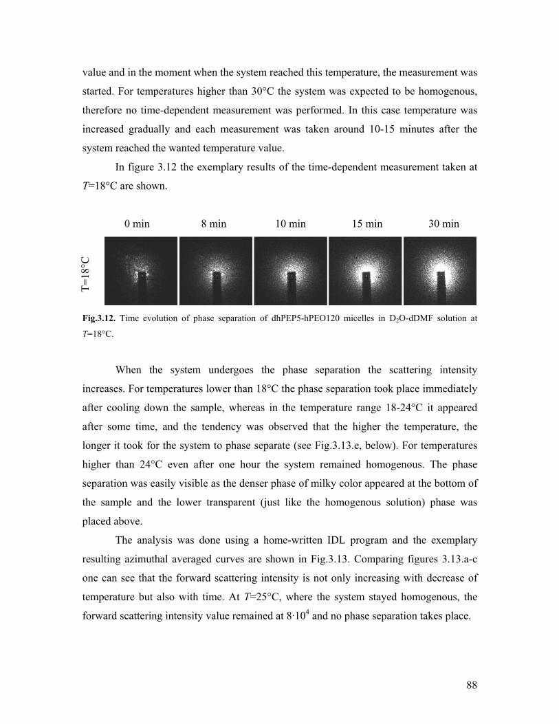
88
value and in the moment when the system reached this temperature, the measurement was
started. For temperatures higher than 30°C the system was expected to be homogenous,
therefore no time-dependent measurement was performed. In this case temperature was
increased gradually and each measurement was taken around 10-15 minutes after the
system reached the wanted temperature value.
In figure 3.12 the exemplary results of the time-dependent measurement taken at
T=18°C are shown.
0 min 8 min 10 min 15 min 30 min
T=
18°C
Fig.3.12. Time evolution of phase separation of dhPEP5-hPEO120 micelles in D2O-dDMF solution at
T=18°C.
When the system undergoes the phase separation the scattering intensity
increases. For temperatures lower than 18°C the phase separation took place immediately
after cooling down the sample, whereas in the temperature range 18-24°C it appeared
after some time, and the tendency was observed that the higher the temperature, the
longer it took for the system to phase separate (see Fig.3.13.e, below). For temperatures
higher than 24°C even after one hour the system remained homogenous. The phase
separation was easily visible as the denser phase of milky color appeared at the bottom of
the sample and the lower transparent (just like the homogenous solution) phase was
placed above.
The analysis was done using a home-written IDL program and the exemplary
resulting azimuthal averaged curves are shown in Fig.3.13. Comparing figures 3.13.a-c
one can see that the forward scattering intensity is not only increasing with decrease of
temperature but also with time. At T=25°C, where the system stayed homogenous, the
forward scattering intensity value remained at 8·104 and no phase separation takes place.

89
2x10⁻⁵ 4x10⁻⁵ 6x10⁻⁵ 8x10-50
1x10⁵
2x10⁵
3x10⁵
4x10⁵
5x10⁵
6x10⁵
Inte
nsity
[a.u
.]
q [Å-1]
T = 18oC 0 min 15 min 5 min 20 min 8 min 30 min 10 min 60 min
2x10⁻⁵ 4x10⁻⁵ 6x10⁻⁵ 8x10-50
1x10⁵
2x10⁵
3x10⁵
4x10⁵
5x10⁵
6x10⁵
Inte
nsity
[a.u
.]
q [Å-1]
T = 20oC 0 min 5 min 30 min 10 min 40 min 15 min 50 min 20 min 60 min
(a) (b)
2x10⁻⁵ 4x10⁻⁵ 6x10⁻⁵ 8x10-50
1x10⁵
2x10⁵
3x10⁵
4x10⁵
5x10⁵
Inte
nsity
[a.u
.]
q [Å-1]
T = 24oC 0 min 15 min 40 min 20 min 50 min 25 min 60 min 30 min 70 min
2x10⁻⁵ 4x10⁻⁵ 6x10⁻⁵ 8x10⁻⁵
2x10⁴
3x10⁴
4x10⁴
5x10⁴
6x10⁴
7x10⁴
8x10⁴
Inte
nsity
[a.u
.]
q [Å-1]
T = 25oC 0 min 60 min
(c) (d)
0 10 20 30 40 50 60
1x10⁵
2x10⁵
3x10⁵
4x10⁵
5x10⁵
6x10⁵
I (q=
1.89
×10-5
Å) /
a.u
.
t [min]
16°C 22°C 17°C 24°C 18°C 25°C 20°C 26°C
(e)
Fig.3.13. Exemplary scattering curves obtained from the time-dependent measurements run at temperature:
(a) 18°C, (b) 20°C, (c) 24°C and (d) 25°C. (e) Forward scattering intensity vs time.
In figure 3.13.e the intensity at lowest measured angle is plotted versus time. For
temperatures lower than 18°C the phase separation appeared immediately after cooling

90
the sample, therefore it is concluded that in this temperature regime spinodal
decomposition is taking place. However, in the temperature range 18-24°C an induction
time is required for phase separation. That is why in this temperature regime the system is
expected to be in the meta-stable state. At higher temperatures the sample stays
homogenous in the time frame of the experiment. As it can be seen from the slope of the
curves in Fig.3.13.e, at T=24°C it takes more than one hour for the system to reach its
final state, for lower temperatures 20-22°C the system decomposes faster (around 30-40
min). At T=18°C the system requires around 20 min to phase separate. In the temperature
regime 18-24°C, just after lowering temperature (t=0) the sample was stable for first 5-
10min. The value of scattered intensity is the same as for the homogenous sample
measured at 25°C and 26°C. At low temperatures 16-17°C the scattered intensity value is
higher than for the homogenous sample from the beginning of the measurement,
however, it does not reach the value of the final state obtained in the temperature range
20-22°C.
3.4.2. Observation of pressure induced phase separation
In order to study pressure induced phase separation, the measurements were
performed for temperatures higher than 30°C because for these temperatures at ambient
pressure conditions the system remains homogenous, and therefore possible phase
separation will be then a pure effect of pressurizing. The pressure-dependent
measurements were done using both, SANS and DLS techniques. In this subchapter their
results will be presented.
3.4.2.1. SANS results
In figure 3.14 the scattering curves for this system are shown. The sample was
measured at two temperatures: 30°C and 40°C. As can be seen directly from the raw data
(see figure 3.14.b), at T=40°C no change in the size of the micelles was observed, as all
the scattering curves overlap. At T=30°C, on the other hand, the macroscopic phase

91
separation was observed after applying pressure of around 800bar. A sequential decrease
of pressure to 750bar did not stop the progressing aggregation.
0.01
1
10
100
1000
I(q) [
cm-1]
q [Å-1]
dhPEP5-hPEO120in D2O-dDMF
T=30oC 30 bar 700 bar 250 bar 800 bar 500 bar 750 bar
0.01
1
10
I(q) [
cm-1]
q [Å-1]
dhPEP5-hPEO120in D2O-dDMF
T=40oC 30 bar 500 bar 1500 bar 2000 bar
(a) (b)
Fig.3.14. I(q) vs q for dhPEP5-hPEO120 in D2O-dDMF at: (a) T=30ºC, (b) T=40ºC.
In this case the core-shell model without any additional contribution was used, as the fit
was performed only for the q-range up to 0.0095Å, since a proper background correction
could not be done (as the scattering of the solvent was not measured). Similarly to the
previous fitting procedure, the change of the scattering length density of the solvent due
to the change in temperature and pressure was taken into account and the aggregation
number, additional radius of the shell (compared to compact) and the smearing parameter
of the shell were fitted. The results are given in the figure below.
0 500 1000 1500 2000200
220
240
350
400
450
500
RM [Å
]
P [bar]
dhPEP5-hPEO120in D2O-dDMF
T=40oC T=30oC
0 500 1000 1500 20000
20
40
200
250
300
350
400
d 3+ [Å]
P [bar]
dhPEP5-hPEO120in D2O-dDMF
T=40oC T=30oC
(a) (b)

92
0 500 1000 1500 2000
4050607080
175
180
185
190
195
Nag
g
P [bar]
dhPEP5-hPEO120in D2O-dDMF
T=40oC T=30oC
0 500 1000 1500 2000
45
50
5572.5
73.0
73.5
74.0
Rco
re [Å
]
P [bar]
dhPEP5-hPEO120in D2O-dDMF
T=40oC T=30oC
(c) (d)
Fig.3.15. Results of fitting with the core-shell model with the constant background for the dhPEP5-
hPEO120 in D2O-dDMF: (a) overall radius, (b) additional thickness of the shell coming from the presence
of the solvent among polymer chains in the micellar corona, (c) aggregation number, (d) the core radius.
The locus of the phase separation is marked with a gray line.
No change in the size of the micelle is observed at T=30°C up to around 600bar and at
T=40°C for the full pressure range. Although the aggregation number and the core radius
are slightly bigger at 30°C, the overall radius (due to bigger contribution of the additional
thickness of the shell, shelld , to the overall radius) is insignificantly smaller. Application
of pressure of around 800bar (at 30°C) induces a phase separation, which is marked in the
plots with a gray line.
3.4.2.2. DLS results
The correlation functions for this sample obtained by DLS are presented in figure
3.16. The experiment was done at 35°C, 30°C and 29°C (in this order). At T=29°C after
applying pressure of 800bar the macroscopic phase separation was observed. The sample
became opaque, however not uniformly in the whole volume, as it can be seen from
Fig.3.16d. Interestingly, the particles did not start to aggregate immediately after
increasing pressure but after around 2 min (which can be seen in Fig.3.16b). Time values
are given only as an approximation, as no proper time-dependent measurements were

93
taken. At this point further studies are required. A slight shift toward longer decays times
in the correlation functions at temperatures 30°C and 35°C observed within the
investigated pressure range is due simply to change of the viscosity and refractive index
of the solvent. The difference of one degree in the temperature, at which the phase
separation appears in SANS and DLS lies in the error range and also might come from
the fact that two different pressure cells are used in both experiments: the thermoelement
mounted in the cell for the light scattering is much closer to the sample (and gives the
uncertainty of temperature measurement of ΔT=0.5°C) than the one used in the cell for
SANS experiment (which gives the error of around 1°C).
1E-4 1E-3 0.01 0.1 1 10 100 100010000
0.0
0.2
0.4
0.6
0.8
1.0
g(2) (t)
-1
t [ms]
dhPEP5-hPEO120in D2O-dDMF
T=29oC 1 bar 700 bar 800 bar
1E-4 1E-3 0.01 0.1 1 10 100 100010000
0.0
0.2
0.4
0.6
0.8
1.0 dhPEP%-hPEO120in D2O-dDMF
T=29oC; P=800bar 2 min 8 min 5 min 11 min
g(2) (t)
-1
t [ms]
(a) (b)
1E-3 0.01 0.1 1 10 100 1000 10000
0.0
0.2
0.4
0.6
0.8
1.0
dhPEP5-hPEO120in D2O-dDMF
T=35oC 1 bar 1000bar
g(2) (t)
-1
t [ms]
(c) (d)
Fig.3.16. The correlation functions for dhPEP5-hPEO120 in D2O-dDMF at: (a) and (b) T=29ºC, (c)
T=35ºC; (d) picture of the sample after applying 800bar at T=29ºC.

94
In order to calculate the hydrodynamic radius of the micelles, the changes in the
refractive index and viscosity of the solvent due to the application of pressure were taken
into account. All the correlation functions obtained for the homogenous solution were
easily fitted with one-exponential decay function. In figure 3.17 the resulting
hydrodynamic radius is plotted versus pressure for each temperature.
0 200 400 600 800 1000
600650700750
1000
1100
1200
1300
1400
Rh [Å
]
P [bar]
dhPEP5-hPEO120 in D2O-dDMF
T=29oC T=35oC T=30oC
0 100 200 300 400 500 600 700 800
200
300
400
500
600
700
800
RM ,
Rh [Å
]P [bar]
dhPEP5hPEO120 in D2O-dDMF Rg from SANS Rh from DLS
(a) (b)
Fig.3.17. (a) The hydrodynamic radius, Rh, received from the DLS measurement, (b) comparison of Rh (at
T=29°C) with RM (at T=30°C) obtained from fitting the SANS data. The gray line indicates the pressure
(for T=29°C) at which the phase separation appears.
First observation similar in both, DLS and SANS, results is that while lowering
temperature, the radius of micelles decreases. Here, the hydrodynamic radius decreases
from Rh≈1160Å at T=35°C to Rh≈1120Å at T=30°C, and eventually to 650Å at T=29°C.
When it comes to pressure-dependency of hydrodynamic radius, at temperatures
higher than 30°C no change in the micellar size was observed in both experiments. This
is similar to the findings for polystyrene of R. L. Cook et al. [75], that the radius of
gyration is invariant with pressure for the polymeric solution in the organic solvents. At
T=30°C applying of pressure up to P=600bar does not change the radius. Further increase
of pressure causes increase of Rh up to around 1350Å at P=1000bar. At even lower
temperature (29°C) increase of the pressure entails the increase of the radius until the
aggregation appears.

95
Comparing this with the SANS results (see Fig.3.17.b) it can be seen that pressure
application does not influence the size of the micelle. It does induce, however, phase
separation, which appears in the DLS experiment as aggregation of micelles (radius
becomes bigger while pressurizing at T=29°C). In the SANS measurement it appeared as
a collapse of the micelle (radius becomes smaller while pressurizing at T=30°C). Due to
the limits in the q-range in the SANS experiment, it was not possible to determine the
size of the aggregates. Comparing the values of hydrodynamic radius at T=29°C and
overall micellar radius of gyration at T=30°C, both at ambient pressure, gives the ratio
1.34h
g
R
R , which is close to predicted value of 1.29 for spherical systems.
3.4.3. Observation of pressure induced phase separation in solution of
homopolymer PEO150 in D2O-dDMF
In order to understand the structural and phase behaviour of a micelle the
structural evidence for the pure polymers that builds the aggregate is needed. Here the
results of measurement of the homopolymer PEO (of a similar molecular weight to the
one in the copolymer that forms micelles) are presented. In figure 3.18 the SANS
scattering curves for the polymer hPEO150 in D2O-dDMF are shown. The sample was
measured at the same temperatures: 30°C and 40°C. Similarly to the previous results for
the dhPEP5-hPEO120 micelles in the same solvent, it can be seen directly from the raw
data that all the scattering curves overlap at T=40°C and so no change in the size of the
polymer coils was observed. At T=30°C, on the other hand, the macroscopic phase
separation was observed after applying pressure of around 800bar. Visual inspection
through the pressure cell windows showed that a “needle”-shaped object was formed
from the aggregating polymers.
The experiment was done as follows: first the sample was measured at T=40°C,
then it was cooled down to T=30°C and the first set of measurements was taken; when
the phase separation appeared, pressure was deceased to P=500bar, the sample was held
at this pressure level and warmed up to 40°C. It took around 10min to increase the

96
temperature, and then it was staying at 40°C for the next 20 min. After that, the
temperature was again decreased (within around 10min) to 30°C in order to repeat the
measurement. The sample was held at these conditions (T=30°C, P=500bar) for the next
half an hour in order to make sure that we reached the state at the beginning of the
measurement. As it can be seen from Figure 3.18c, after 26min of warming up the sample
reached its beginning state. The difference between first and the second set of
measurements can be seen for at P=800bar: in the first one – the increase of the pressure
form 700 to 800bar results in the increase of the intensity at small q from around 0.9 to
5.8cm-1. In the second one the increase of the pressure form 750 to 800bar results in the
increase of the intensity at small q from around 0.9 to 1.3cm-1. This difference can be
explained by the time dependency of the phase separation process that was observed for
the micellar system in the same solvent using DLS (see Fig.3.16.b)
0.01 0.1
0.1
1
I(q) [
cm-1]
q [Å-1]
PEO150 in D2O-dDMF
T=40oC 30 bar 250 bar 1500 bar 500 bar 2000 bar 1000 bar 2500 bar
0.01 0.1
0.1
1
10
I(q) [
cm-1]
q [Å-1]
PEO150 in D2O-dDMF
T=30oC 30 bar 800 bar 500 bar 2000 bar 700 bar
(a) (b)

97
0.01 0.1
0.1
1
10
I(q) [
cm-1]
q [Å-1]
PEO150 in D2O-dDMF
T=38-40oC; P=500bar 4 min 12 min 18 min 15 min 26 min
T=30oC; P=500bar 1 h 20 min first measurement
0.01 0.1
0.1
1
10
I(q) [
cm-1]
q [Å-1]
PEO150 in D2O-dDMF
T=30oC 500 bar (first) 500 bar 850 bar 750 bar 900 bar 800 bar 1000 bar
(c) (d)
Fig.3.18. I(q) vs q for hPEO150 in D2O-dDMF at: (a) T=40ºC, (b) and (d) T=30ºC, (c) warming up of the
sample.
Here, the determination of the radius of gyration will be given. It can be obtained
simply using the Zimm approximation:
2 21 1
1( ) ( 0) 3
gR q
I q I q
, (Eq.3.26.)
where both parameters, forward scattering intensity I(q=0) and radius of gyration Rg were
fitted.
On the other hand, this can be compared with:
2 2
22 2
11 1 2
( ) 3gR qM
A McI q cK V
, (Eq.3.27.)
where: c is the concentration of the polymer solution, K – the contrast (the difference in
scattering length density between the particle and the solvent), V – the polymer volume
[96]. Assuming no interactions between particles (second virial coefficient, A2=0; very
dilute solution), one can estimate I(q=0). This way it is possible to check if the data
reduction and the fitting were done properly. For the investigated PEO solution, the value
of intensity at q=0 from Eq.3.27 it is expected to be around 1.47cm-1, taking the
molecular weight of around 130kg/mol, obtained from GPC, the polymer density of
1.125g/cm3, and the scattering length densities hPEO =6.37·109cm-2 of the polymer and
0 =6.34·1010cm-2 of the solvent. Fitting the scattering curves from SANS experiment

98
with the Zimm function (Eq.3.26) gave us the value of I(0) always around the expected
one, which ensures that the fitting procedure was done correctly and moreover, the values
of radius of gyration obtained from the fitting procedure are correct.
The results are shown in figure 3.19. Although it was still possible to fit the data
for P=800bar at T=30°C with the Zimm function, it cannot be taken into account, as here
the phase separation appeared and the approximation A2=0 is not valid anymore, and the
I(q=0) was twice bigger than the one predicted from Eq.3.27. Similarly to the results for
the dhPEP5-hPEO120 micelles in the same solvent, there is no change in the radius of
gyration until the phase separation occurs.
0 500 1000 1500 2000140
150
160
170
180
190
200
210
220
230
hPEO150 in D2O-dDMF
T=40oC T=30oC (first) T=30oC (second)
Rg [Å
]
P [bar]
Fig.3.19. The radius of gyration, Rg, plotted versus pressure. The gray line indicates the pressure (for
T=30°C) at which the phase separation appears.
3.5. Discussion
In this subchapter the discussion of the results for the temperature- and pressure-
dependent behaviour the dhPEP5-hPEO120 micelles in both solvents will be given for,
respectively, the water dispersion and the water-DMF mixture.

99
3.5.1. Temperature- and pressure-induced shrinkage of dhPEP5-
hPEO120 in D2O
For the investigated water dispersion, the gyration and hydrodynamic radii were
estimated using light and neutron scattering techniques at ambient conditions (T=20°C,
atmospheric pressure). The results are summed up in the table below.
Table 3.6. The values of gyration and hydrodynamic radii of dhPEP5-hPEO120 micelles in D2O at T=20°C
and ambient pressure obtained from SANS, SLS and DLS experiments.
experimental
technique
radius of gyration,
Rg [Å]
hydrodynamic radius,
Rh [Å]
volume fraction,
Φ [%]
SANS 686 – 0.33%
SLS 521 – 0.066%
DLS – 835 0.066%
The difference in the resulting values of gyration radius from SANS and SLS is
due first of all to different fitting models that were used. SANS data was modeled with
core-shell and Beaucage functions, and SLS data was fitted using Guinier approximation
(first term in Beaucage model, see Eq. 3.23). The other reason lies in different origin of
scattering process while using light and neutrons as incident beams. Light is scattered due
to local fluctuations in the dielectric constant of particles, whereas neutrons are scattered
at the nuclei of atoms. What differs both techniques is also the issue of contrast between
the polymer chains and the solvent. In light scattering experiment contrast comes from
the difference in refractive indices of particles and solvent. When this difference is too
small, no (or very weak) intensity fluctuations will be recorded, but in case it is too big,
sample appears opaque, which spoils the experiment. At ambient conditions the refractive
index of the polymer (PEO) is 1.4539 and the refractive index of solvent (D2O) is 1.3284.
It was found out that the dilution was required in order to receive transparent sample. On
the other hand, in neutron scattering experiment the contrast is determined by the
difference in scattering length densities of solute and solvent. At ambient conditions the
values of scattering length density are 6.37·109cm-2 for PEO and 6.37·1010cm-2 for D2O.

100
This difference of one order of magnitude is an advantage in neutron scattering
experiment and therefore makes this technique more suitable for investigation of this
system, and the results more trustworthy.
The relation of both radii, gyration and hydrodynamic, from light scattering
experiments was found to be 1.6h
g
R
R , and comparison of hydrodynamic radius with the
overall micellar radius from SANS gives the ratio 1.22h
M
R
R . The later is close to the
expected value (around 1.29) for spherical objects.
Comparing these results with previous findings of Willner et al. [97] for exactly
the same polymeric micelles, one sees big discrepancy, although the same model (core-
shell geometry) was used to fit the SANS data, see table 3.7. The aggregation number is
an order of magnitude smaller than the one obtained by Willner et al. [97], and both radii,
Rcore and RM are around twice smaller. The possible explanation of such a big
disagreement lies in the aging of the sample (one has to note that here exactly the same
diblock copolymer was used 10 years after experiments performed by Willner et al. [97]),
however, the recent GPC test did not reveal sufficient change in molecular weight of the
block copolymer.
Table 3.7. Comparison of the micellar characteristic with the results of Willner et al. [97].
Nagg Rcore [Å] RM [Å] source
67 52 686 here
870 120 1170 Willner et al. [97]
Coming to the temperature- and pressure-dependence of the investigated system
in water, a decrease in the overall micellar radius, RM, was found using SANS technique.
The biggest contribution to the overall radius is due to the additional thickness of the
shell, shelld , which represents the thickness of the shell compared to the compact one. In
other words, it includes presence of the solvent among polymer chains building the
micellar corona. Its temperature- and pressure-dependent behaviour is in agreement with
the previous findings [51-[60] about breaking of hydrogen bonds between water

101
molecules and the oxygen atoms in the polymer chains while heating up or pressurizing
the sample, which causes coiling of the polymer. Further increasing temperature to LCST
(around 100°C) would cause phase separation. Cooling the system below the room
temperature (the measurement at T=9°C) still leads to swelling of the micellar corona, but
the difference between the values of RM and shelld measured at 9°C and 20°C is not
significant. This is in agreement with the reduction of the solvent quality of water for
PEO below room temperature, as reported in [59]. It can be assumed that for even lower
temperatures the swelling of PEO chains will be suspended and eventually the phase
separation will be observed after crossing the upper critical solution temperature (UCST).
Contrary to the micellar radius and shelld , the aggregation number increases while heating
up and at lower temperatures (9°C) it increases also with pressurizing. The core radius,
which depends solely on Nagg (see Eq.3.20), does not change significantly with
temperature (from 50Å at T=9°C to 57Å at T=70°C) and pressure, as it depends on
aggregation number as a cubic root. However, a small increase while heating can be
observed, and at lower temperatures (9°C) it increases also with pressurizing. This is in a
contradiction with previous studies [73,[98,[99], which have shown that the PEP-PEO
micelles in water are kinetically frozen (no unimer exchange between micelles was noted
even at high temperatures and for long time observations). Here it was found that the
value of Nagg in the temperature range 9-70°C varies of around 30%. This inconsistency
can be decided by performing SANS experiment in so-called core contrast, where the
mixture of the protonated and deuterated solvents (in this case H2O and D2O) is prepared
that the scattering length densities of polymer building the corona block and the solvent
are equal ( hPEO solvent ). Under these conditions the scattering signal comes only from
the micellar core and its possible change in size and composition induced by the variation
of temperature and pressure can be obtained straightforwardly.
Another feature of the temperature- and pressure-dependent behaviour of this
dispersion is that there is no straightforward dP/dT relation as it was observed for the
sticky hard sphere system investigated by Vavrin et al. [17]. To test the dP/dT
proportionality, a 2nd polynomial fit, 21 2MR A B P B P was performed for the

102
values of the overall micellar radius measured at each temperature, which is shown in
Fig.3.20 as red lines.
0 500 1000 1500 2000 2500450
500
550
600
650
700 PEP5-PEO120 in D2O
9oC 50oC 20oC 70oC
RM [Å
]
P [bar]
Fig.3.20. The 2nd polynomial fit (red lines) of the pressure-dependency of the overall micellar radius.
The resulting values of the coefficient B1 and B2 are given in the table below. At
intermediate temperatures (20 and 50°C) the absolute value of B2 coefficient is smaller
than at 9°C and 70°C. On the other hand, the absolute value of the coefficient B1
increases while lowering temperature from 70°C to 20°C, and then decreases again while
cooling below room temperature.
Table 3.8. Coefficients from 2nd polynomial fit of the pressure-dependent RM values for temperatures: 9,
20, 50 and 70ºC.
A [Å] B1 [Å/bar] B2 [Å/bar2]
9ºC 694.14025 -0.01779 -9.3937·10-6
20ºC 680.36538 -0.02171 -6.97517·10-6
50ºC 621.05358 -0.01736 -6.72136·10-6
70ºC 538.51134 -0.00374 -10.4969·10-6

103
The complex dP/dT relation can be also seen in Figure 3.9.f, where the temperature and
pressure conditions at equal micellar radius are given. Also here, there is no linear
relation. The micelles, unlike the octadecyl grafted silica particles, are more complex
system, and its response will come from the reaction of both polymers, PEP and PEO, to
the change of temperature and/or pressure. One should distinguish two contributions to
the temperature and pressure behavior. Firstly, at higher temperatures and elevated
pressure water becomes a poorer solvent for PEO, which causes coiling of this polymer,
and hence a decrease in the micellar radius. Secondly, interfacial tension between PEP
and water increases, which then results in bigger Nagg and formation of bigger micellar
core, and hence Rcore increases. As the PEO chains are much longer than PEP in this
system, the effect of folding of PEO and its influence on the overall micelar radius will
be more pronounced. Hence, the first contribution dominates the behaviour of PEP-PEO.
Applying pressure acts as increasing temperature, causing a decrease of the micellar
radius.
On the other hand, the shrinking of the micelles was not observed in the DLS
measurement, but there are difficulties with interpreting this data set as the solution is
highly polydisperse so that the resulting values of hydrodynamic radii were obtained with
uncertainty of more than 10%.
3.5.2. Temperature- and pressure- induced phase separation of
dhPEP5-hPEO120 and hPEO150 in D2O-dDMF
The temperature at which phase separation occurs at ambient pressure conditions
was determined by performing SALS experiment. It was found that for temperatures
lower than 18°C the sample undergoes a demixing process immediately after cooling,
while in temperature range 18-24°C it appears after certain time, and the higher the
temperature is, the longer it takes for the system to phase separate. At 25°C the system
becomes stable. The measurement at atmospheric pressure was done in order to find the
temperature range in which the system is stable, so that the pressure-dependent

104
experiment will be run in this regime. Then the possibly observed phase separation will
be induced solely by pressure.
In pressure-dependent SANS and DLS experiments for the investigated systems
in equi-molar D2O-dDMF mixture we observe firstly, that the overall radius of micelles
in this solvent is smaller than in water solution, which is related to the compatibility of
both polymers, PEP and PEO, with DMF. Secondly, until the phase separation no change
in radius of micelle or polymer coil occurs while applying pressure. For both systems,
PEP-PEO micelles and PEO homopolymer, phase separation sets in at the same
temperature and pressure conditions. Moreover, pressure induced phase separation does
not set in immediately, as it was shown with the DLS measurement (Fig.3.16.b), where
the second decay of the correlation function, corresponding to the diffusion time of
formed aggregates, appears only a few minutes after applying pressure. Finally, the other
feature obtained from the SANS measurement (see Fig.3.14.a) is that once phase
separation sets in, lowering of pressure will not reverse the demixing process. The sample
was brought back to the homogenous state by raising the temperature. In this subchapter,
the comparison of the results of the both systems, PEP-PEO micelles and PEO
homopolymer, will be given, and the observation of the phase separation will be
discussed.
As already mentioned in chapter 3.1, the addition of DMF results in a substantial
decrease of the interfacial tension between PEP and the solvent. This causes reduction of
the aggregation number as compared to that in pure water [73]. For the micelles in water-
DMF the aggregation number in the range of Nagg=40-50 was found at T=40°C and
Nagg≈55 at T=30°C (before the phase separation set in). Micelles in pure water have the
aggregation number in the range of Nagg=70-80 in the temperature range of 20-50°C. This
is in agreement with the results of Lund et al. [73]. The previous studies [73,[98,[99] on
the PEP-PEO system in water-DMF mixtures reveal the unimer exchange process at
higher temperatures, during which the equilibrium structure was maintained [98].
However, in the experimental conditions applied here, the presence of exchange process
is not expected and therefore, no change in the aggregation number should be observed.
As expected, Nagg is only slightly smaller at T=30°C than at 40°C, which is due to small

105
decrease of the interfacial tension between PEP and the solvent with increasing
temperature. It stays unaffected by the application of pressure until phase separation sets
in.
On the other hand, the addition of DMF causes also the shrinking of the corona
comparing to the one in pure water solution [73]. The theory of starlike micelles predicts
the dependence of the corona thickness M coreD R R on aggregation number:
1/5 3/5agg AD N N . (Eq.3.28.)
Compensating the reduction in corona size for the reduction in Nagg (which was done by
scaling D by 1/5aggN according to Eq.3.28), revealed the relative shrinkage of about 20%
for the PEP1-PEO20 micelles [73]. For the system investigated here, which is even more
asymmetric while the fraction of PEO compared to PEP chains is even higher, the drop in
1/5/ aggD N from pure water to water-DMF solution is also expected. One cannot make a
direct comparison as both samples were measured at different temperature conditions.
Nevertheless, for micelles in pure water at ambient pressure 1/5/ aggD N stays in the range of
265-235Å in the temperature range of 20°C-50°C, whereas for the same system in water-
DMF mixture 1/5/ aggD N has the value of 195-208Å in the temperature range 30°C-40°C.
On average it gives also the drop in 1/5/ aggD N of around 20% from pure water to equi-
molar water-DMF solution. The contribution to the overall micellar radius coming from
PEO chains does not change the overall micellar radius with pressure, which means that
pressurizing of the sample up to 2500bar at 40°C and up to 700bar at 30°C does not
influence the conformation (size) of the PEO coils. This was confirmed by the reference
measurement of the PEO homopolymer of similar molecular weight to the one in the
block copolymer. It proved that the PEO polymer size stays unchanged under the
pressure up to 2500bar at 40°C and up to 700bar at 30°C.
Second remark is related to the unchanged radii of PEP-PEO micelles and PEO
homopolymer under action of pressure until phase separation sets in. This is different
from the observation of micellar radius in water solution, where the decrease in the radius
was observed while approaching LCST. This difference is probably due to the micellar

106
conformation in both solvents. In water, which is good solvent for PEO, the micellar
corona is swollen. Hence, changes in solvent quality will be easily seen in the decrease of
the corona thickness and therefore, in the micellar radius. In water-DMF solution, which
is poorer solvent for PEO than water, the micellar corona is more compact. That is why
any change in its thickness or overall micellar radius is harder to be observed.
For the homopolymer we observed the phase separation at exactly the same
temperature and pressure conditions as for the micelle system, which means that phase
transition of the micellar system is governed by PEO behaviour. In future, the kinetics of
the phase separation can be studied more extensively, as it was shown here that it does
not appear immediately after pressurizing. Because it takes a few minutes after applying
pressure, it is rather hard to investigate it in details with SANS technique, as within this
time interval data is usually accumulated and thus averaged. In order to have better time
resolution, the so-called pressure jump technique can be used. In this mode after applying
pressure, scattered intensity is recorded in short time-slices. This procedure is repeated
several times and eventually the signal from each short time range is averaged from all
repetitions.
3.6. Conclusions
To conclude, the behaviour of the PEP5-PEO120 micellar system in pure water
and equi-molar water-DMF mixture is governed mostly by the contribution coming from
the reaction of PEO chains to the change of temperature, pressure or solvent composition.
Temperature- and pressure-dependent shrinking of micelles in water is attributed
to a decrease of the solvent quality of water for PEO. As the investigated micelles are
highly asymmetric and consist mainly of PEO, its reaction to the variation of temperature
and pressure shields the contribution coming from PEP behaviour in water.
The micellar radius of the same system in the water-DMF solution did not change
while pressurizing until a phase separation appeared. We think this is due to the fact that
addition of DMF to the solvent caused formation of smaller and very compact micelles.

107
This has two causes: firstly, the interfacial tension between PEP and the D2O-dDMF
solution is much smaller than for pure water, and secondly, presence of DMF decreases
the solvent quality for PEO and result in coiling of the polymer. The phase separation did
not take place immediately after applying certain pressure but it occurred after a few
minutes.
In the case of PEP-PEO micelles in water applying pressure has similar effect as
increasing temperature, although there is no simple linear dP/dT relation. In the case of
PEP-PEO micelles in water-DMF solution applying pressure acts as lowering of
temperature.
In future work the attention could be paid to the kinetics of phase separation under
pressure and the attempt to determine the dP/dT relation could be made. Having
characterized the effect of temperature and pressure on the form of single micelles, we
can now also start to study the effect of these parameters on concentrated solutions.

108
PART II

109
4. The temperature dependence of the poly(ethylene-co-propylene)
(PEP) copolymer macroscopic viscosity studied by Fluorescence
Correlation Spectroscopy (FCS)
4.1. Introduction
There is an ongoing discussion on the problem of nano- and macroviscosity of
polymer solutions. The type of measured viscosity depends on the size of the particles
probing polymer solutions: while diffusing, small objects (of sub-nanometer size) are
expected to experience the viscosity of a solvent in which the polymer is dispersed,
whereas the diffusion of objects larger than the polymer size is supposed to depend on the
macroscopic viscosity of the whole solution. As it was found by Holyst et al. [100], the
length scale at which the crossover from nano- to macroscopic viscosity is observed is
related to the polymer radius of gyration.
The goal of these experiments was to find the correlation between temperature
dependency of: the polymer macroscopic viscosity and the diffusion time of a nanoscopic
probe diffusing between the polymer chains, using a temperature cell combined with the
Fluorescence Correlation Spectroscopy (FCS) setup. In the work of Holyst et al. [100]
the viscosity of the polymer dispersion was changed by varying the polymer
concentration. It can be also done using temperature as variable. In FCS technique the
self diffusion time of fluorescent (or fluorescently labeled) particles is measured.
Determining the size of the confocal volume by measuring diffusion time of a standard
sample (for example rhodamine), the diffusion coefficient of the investigated sample can
be obtained. If the Stokes-Einstein (Eq.3.11 and 3.12) relation is valid for a measured
system, the diffusion time obtained in FCS experiment can be used to calculate the
dispersion viscosity.
Here, the temperature dependent diffusion times of a fluorescent dye, rubrene,
dissolved in a poly(ethylene-co-propylene) copolymer were investigated. In this case
there is no solvent used, rubrene is diffusing only among polymer chains. Therefore the

110
variation of diffusion times with temperature is expected to depend solely on the
temperature induced changes in the macroscopic viscosity of the polymer.
4.2. Experimental section 4.2.1. Materials
The poly(ethylene-co-propylene) copolymer PEP6, provided by Lutz Willner and
Jürgen Allgaier, was used. The number denotes approximated molecular weight in
kg/mol. The details of the synthesis procedure were published elsewhere [79]. This
particular polymer was chosen because of its low glass transition temperature,
62gT C . The fluorescent dye rubrene (5,6,11,12-tetraphenylnaphthacene; Sigma
Aldrich R2206), which structure is schematically shown in Fig.4.1.a, was used in the
experiment. The absorption and fluorescence spectra of 20μM solution of rubrene in
cyclohexane at room temperature taken from Bayrakçeken [102] are given in Fig.4.1.b as
an example. The size of rubrene (the length of the tetracene backbone) molecule is of
order of 1nm.
(a) (b)
Fig.4.1. (a) Rubrene structure [101]; (b) absorption and fluorescence spectra of Rubrene in cyclohexane at
room temperature [102].

111
In order to prepare the 1nM solution of rubrene in PEP6 first 1g of PEP6 was
dissolved in toluene and 0.053g of rubrene, which would correspond to 0.1mM
concentration in PEP6, was also dissolved in toluene. The solution of rubrene in toluene
was then diluted gradually to obtain the amount of rubrene that would correspond to 1nM
concentration. This final solution of rubrene in toluene was then added to PEP6 in
toluene and mixed using magnet stirrer while keeping the sample on heating plate in
order to let the toluene evaporate. In order to remove the toluene properly, the sample
was kept in a vacuum oven (Heraeus vacutherm).
4.2.2. Viscosity measurement
The viscosity measurements of: the investigated sample consisting of PEP6
polymer with addition of 1nM concentration of the fluorescent dye rubrene, and the pure
polymer PEP6 were performed using the commercial rheometer Physica MCR 501
(Anton Paar). The viscosity was measured in the temperature range 0-70°C in steps of
5°C at shear rates of 0.01-1s-1, at 3 points per decade. This low shear rate range was
chosen in order to obtain the zero shear viscosity, defined by:
0 0
"lim
G
, (Eq.4.1.)
where "G is the dynamic loss modulus and ω – the angular frequency.
Caution has to be taken concerning the measuring time. In order to be sure that the
viscosity reaches a stationary value the measuring time per data point has to be long
enough. Here it was set to 60 seconds. The temperature scan was done both ways: by
warming up and cooling down the samples in order to check if any change in viscosity
depending on the way of varying temperature will be observed. Before starting any new
measurement there was given 10 minutes of a waiting time for the sample to equilibrate
after each change of the temperature. The results are presented in Fig.4.2.

112
0.01 0.1 1
10
100
1000
70oC
60oC
50oC
40oC
30oC
20oC
10oC
0oC
PEP6 + 1nM Rubrenewarming cooling
[P
a*s]
shear rate, [1/s]•
0.01 0.1 1
10
100
1000
70oC
60oC
50oC
40oC
30oC
20oC
10oC
0oC
•
PEP6: warming cooling
[P
a*s]
shear rate, [1/s]
(a) (b)
Fig.4.2. Results of the zero shear viscosity measurement of: (a) the sample consisting of PEP6 and rubrene
used in diffusion time measurement (using FCS technique) and (b) the pure polymer PEP6.
In the chosen shear rate regime the values of the viscosity at each temperature are
constant. This is the proof of obtaining zero shear viscosity values.
4.2.3. Fluorescence Correlation Spectroscopy (FCS)
In FCS experiments the temporal fluctuation of the fluorescence intensity, δI(t),
are measured. These fluctuations arise from the fluctuations in the quantum yield of a dye
or from the constant motion of fluorescent molecules in the observation (confocal)
volume. Here, the later will be discussed. The fluctuations of the fluorescence intensity at
any arbitrary time t are analyzed with respect to its self-similarity after the lag time, τ, in
the form of autocorrelation function:
1( ) ( ) ( ) lim ( ) ( )
2
T
TT
G I t I t I t I t dtT
(Eq.4.2.)
Here, I(t) denotes the collected fluorescence intensity, <I> its mean value and δI(t) the
deviation from the mean value. The definition of the autocorrelation function is given for
one particular interval τ, but the complete autocorrelation function specifies G(τ) for
every τ. The fluorescence intensity at certain time t can be written as ( ) ( )I t I I t ,
therefore the autocorrelation function:

113
2( ) ( ) ( )G I I t I t (Eq.4.3.)
has a constant term 2
I and a time dependent part, which contains information about the
kinetics of a chromophore in an investigated sample. In the fitting program for data
analysis the autocorrelation function is given in the normalized form:
2 2
( ) ( )( )ˆ ( ) 1I t I tG
GI I
. (Eq.4.4.)
Assuming the separation of fluorescence time F and translational diffusion time D
( F D , which usually is the case), the contribution of the translational self diffusion to
the autocorrelation function is described as:
1 1/2
2 2
1 4 4ˆ ( ) 1 1 1xy z
D DG
N
, (Eq.4.5.)
where ωxy and ωz denote the distances from the centre of the laser beam focus in the
radial and axial direction, respectively, at which the detected fluorescence intensity drops
by a factor of e2 compared to its peak value. The ratio ωz/ωxy describes the shape of the
observation volume and is called the structure parameter. In Eq.4.5, N is the mean
number of labeled particles within the observation volume (equal to π3/2ωxy2ωz), and D
stands for the translational self diffusion coefficient of the fluorescent molecules equal to:
2
4xy
D
D
, (Eq.4.6.)
where D is the self diffusion time (the decay time of the autocorrelation function). Here,
the rotational diffusion is omitted because it plays a role for rod-like particles and the
fluorescent dye used in the experiment, rubrene, has a round shape. Analysis of the
rotational diffusion can be found elsewhere [103].
So far, it was assumed that the fluorescent properties of the chromophore do not
change while traversing the laser focal volume, which does not hold for real dyes and
higher excitation powers, as the molecules can enter and leave their triplet state. The
chromophore needs comparably long time to relax back from the triplet to the ground
state. During this time, the dye cannot emit any fluorescent light and appears dark. The
intra- and intermolecular reactions giving rise to fluorescence fluctuations happen in the

114
time-scales much faster than the diffusion of particles. Therefore, a simple separation of
the dynamics is possible, and it leads to the autocorrelation function form of:
( ) ( ) 1 exptotal DT
G G T T
, (Eq.4.7.)
where GD(t) is expressed by Eq.4.5, T refers to the fraction of particles that are in the
triplet state, and T is the triplet state life-time. The more detailed description can be
found elsewhere [104]. The presence of triplet states was taken into account in the fitting
procedure in the FCS data analysis.
The experiments were performed using a commercial FCS spectrometer
ConfoCor 2 (Zeiss, Jena, Germany). It is shown schematically in Fig.4.3, and the main
modules it consists of are: the laser unit, the avalanche photodiode detector box, the
detection unit with the high numerical aperture objective and a PC with the software
controlling the machine operation, collecting and analyzing data. The three lasers give the
possibility of choosing excitation length: the argon-ion laser (Spectra Physics, emission
lines at 458nm, 488nm and 514nm, maximal power 25mW, water cooled) and two
helium-neon lasers (Spectra Physics, λ=543nm, 5mW and Spectra Physics, λ=633nm,
15mW). The helium-neon laser was used in the experiment with the wavelength of
λ=543nm and 70% excitation transmission. Detection unit contains the main parts for
illumination with laser light and for the detection of the fluorescence light. A parallel
beam from collimator is reflected by the main beam splitter and guided to the microscope
to the high aperture objective, which collects also the fluorescent light emitted by
molecules in the sample. The focal spot size is in the femtoliter volume range.
Fluorescent light (marked with red lines in Fig.4.3) with a longer wavelength than the
excitation light (marked with blue lines in Fig.4.3) can pass the main beam splitter
(dichroic mirror), which blocks all reflected excitation light. The pinhole optics (a high
corrected lens) focuses the fluorescent light from the focus image of the sample onto the
pinhole which acts as the field diaphragm. This type of confocal setup discriminates all
out-of-focus originating signals. Therefore only the light coming from the confocal focus
volume in the sample enters the fibre guide to the ADP detector (SPCM-AQR-13-FC,

115
EG&G, Canada). The more detailed description was given by Jankowski and Janka
[105].
Fig.4.3. Schematic representation of the experimental setup for Fluorescence Correlation Spectroscopy –
ConfoCor 2.
The sample was situated in the home-built temperature cell connected to the 330
Autotuning Temperature Controller (Lake Shore), which sets the temperature with
accuracy of 0.05°C. The scheme of the temperature cell is shown in figure 4.4. Before
starting any new measurement there was given at least 15min of a waiting time for the
sample to equilibrate after each change of the temperature.

116
Fig.4.4. Temperature cell used in the FCS experiment.
4.3. Results and discussion
The data from FCS experiment were analyzed using a program written by Jacek
Gapiński, FCS_fit, which allows fitting autocorrelation functions using Eq.4.7. A single
decay fitting model was used (second amplitude, A2, was always set as 0), however,
taking into account bleaching effect and presence of triplet state. The fixed parameters
were structure parameter z
xy
SP
(set as 20) and base line (set as 1).
The reason to put such a high value for the structure parameter is that the 40x0.6
dry objective was used in the experiment. This objective was chosen because of its long
working distance 3.65mm. An objective used in this experiment cannot approach the
sample container due to the shape of the temperature cell and its isolating cover. On the
other hand, using dry objectives for the observation of wet specimens has a disadvantage
of aberrations due to the refractive index mismatch. This results in a focal shift between
the nominal focal position (defined as the geometrical focus in a perfectly matched
system) and the actual focal position. The difference between the refractive indices of the
immersion and embedding media is larger than for other objectives, and that is why
focusing even a few micrometers into the sample will also cause in a severe drop of
intensity and resolution. This can be avoided by adjusting the correction collar [106].

117
In order to determine the size of the confocal volume (in other words, structure
parameter) obtained using the 40x dry Olympus objective of (NA=0.6, WD=3.65mm),
the model system, like for example rhodamine 6G dispersed in water, can be measured.
Using standard water immersion C-Apochromat objective from Zeiss for investigation of
water dispersions gives the structure parameter value of around 5. However, using a dry
objective results in elongated shape of the confocal volume in z-axis direction due to
aberrations caused by refractive index mismatch. The autocorrelation function of
rhodamine 6G dispersed in water measured with this objective is given in figure 4.5.
10-1 100 101 102 103 104 105 106 107 108
1.0
1.5
2.0
2.5
3.0
G(
)
t [s]
N = 0.76T = 0.38T = 0.36D = 88.73SP = 22.172 = 243.56
Fig.4.5. Exemplary autocorrelation function of Rhodamine 6G in water obtained from measurement, in
which the 40x, NA=0.6 dry objective (Olympus) was used.
Red line represents fit of the autocorrelation function and the values of fitted
parameters are given in the inset. It gave the value of SP around 20 and it will be used as
a fixed parameter in fitting of the autocorrelation functions of the investigated system.
Moreover, substituting Eq.4.6 to Eq.4.5:

118
1/21 2
1 1/2
2
1ˆ ( ) 1 1 1
11 1 1 ,
xy
D D z
D D
GN
SPN
(Eq.4.8.)
shows that when structure parameter SP is large, the expression in the second bracket in
Eq.4.8 goes to zero, but the diffusion time D and therefore diffusion coefficient remains
unchanged as long as the horizontal radius of the confocal volume xy is not affected by
aberrations due to the refractive index mismatch.
The exemplary autocorrelation functions of the rubrene in PEP solution with their
fits (marked with red lines) obtained at three different temperatures: 40, 70 and 90°C are
shown in figure 4.6.
100 101 102 103 104 105 106 107
1.00
1.02
1.04
1.06
1.08
1.10
PEP6 + 1nM rubrene T = 40oC T = 70oC T = 90oC
G(
)
t [s]
Fig.4.6. The exemplary autocorrelation functions from FCS obtained from measurements done at T=40°C,
70°C and 90°C with fits marked as red lines.
In this figure one can see the shift of the autocorrelation function decays to longer
times while decreasing the temperature. This represents the slowing down in the motion

119
of the rubrene particles in the suspension of PEP while cooling. Moreover, plotting the
sample viscosity and diffusion times values versus temperature (see Fig.4.7) the same
tendency (slope of the curves) can be observed. This simply means that the slowing down
of the rubrene motion is solely due to the increase of the polymer viscosity while
lowering temperature.
0 10 20 30 40 50 60 70 80 90
104
105
106
0 10 20 30 40 50 60 70 80 90
10
100
1000
diff [
s]
diff from FCS
PEP6 warming cooling
PEP6 + 1nM Rubrene warming cooling
[P
a*s]
T [ oC]
Fig.4.7. Results of the viscosity and the diffusion time measurements.
Further on, in figure 4.8 logarithm of the viscosities of: pure PEP6 (blue squares), 1nM
rubrene in PEP6 solution (black squares) and logarithm of the diffusion time (red dots)
versus temperature are plotted. For these curves fitting with the 2nd polynomial function
A+B1·T+B2·T2 (green lines) was done. This gives quantitative estimation of the slope of
all of the curves.

120
-10 0 10 20 30 40 50 60 70 80 90 1003.0
3.5
4.0
4.5
5.0
0.5
1.0
1.5
2.0
2.5
3.0
log di
ff
1nM rubrene in PEP diff
2nd polynomial fit
T [ oC]
viscosities:PEP61nM rubrene in PEP
2nd polynomial fit
log
Fig.4.8. Logarithm of viscosities of pure PEP6 and 1nM rubrene in PEP6 and logarithm of diffusion time
of rubrene in PEP6 versus temperature with their 2nd polynomial fits.
The obtained values of the 2nd polynomial function coefficients are summed up in the
table 4.1. As it can be seen, the values of B1 are around -0.044, and the values of B2 are
around 2·10-4 for all of the curves, which is a proof of the same tendency in temperature
behaviour of both, diffusion time of rubrene and the viscosity of PEP polymer.
Table 4.1. Coefficients from 2nd polynomial fit of temperature-dependent PEP6 and 1nM rubrene in PEP6
viscosity: η(P)=A+B1·T+B2·T2. Coefficients from 2nd polynomial fit of temperature-dependent diffusion
time of rubrene in PEP: diff = A+B1·T+B2·T2.
viscosity
sample: A Pa s B1 Pa s
C
B2 2
Pa s
C
PEP6 2.61668 -0.0438 1.96978·10-4
1nM rubrene in PEP6 3.07794 -0.04706 2.09242·10-4
diffusion time
sample: A s B1 s
C
B2 2
s
C
1nM rubrene in PEP6 6.11511 -0.04431 1.87349·10-4

121
Additionally, the difference between the viscosity of the 1nM rubrene in PEP6
and the viscosity of the pure polymer was observed. This can be caused by the sample
preparation procedure because the sample was held in vacuum conditions in order to
remove toluene in which both components were dissolved primarily to distribute the dye
uniformly in the polymer suspension. Probably the remains of solvents after
polymerization process were also removed this way, and that causes higher viscosity of
the PEP6 with rubrene solution than the polymer itself. Nevertheless, the tendency of
increasing viscosity while decreasing temperature for both samples is the same: black and
blue points, corresponding to viscosities of 1nM rubrene in PEP6 solution and pure
PEP6, respectively, form curves of the same slope, which can be seen in Fig.4.7 and 4.8.
5.4. Conclusions and outlook
To conclude, the correlation between the temperature dependence of: the
poly(ethylene-co-propylene) (PEP) macroscopic viscosity and the diffusion time of a
nanoscopic probe represented by rubrene molecules diffusing between polymer chains
was found. The macroscopic viscosities of pure polymer PEP and the investigated sample
consisting of 1nM rubrene in PEP dispersion were determined by rheological
measurement at zero shear viscosity conditions. The temperature-dependent values of
diffusion time of rubrene were obtained from FCS measurement using the home-built
temperature cell. Both quantities, polymer viscosity and rubrene diffusion time, show the
same tendency with temperature (see Fig.4.8), which means that the temperature
dependency of rubrene diffusion depends solely on macroscopic viscosity of the polymer,
in which it is dissolved, as it was predicted based on findings of Holyst et al. [100].
Also the home-built temperature cell for FCS set up was tested here as well. It
requires using long working distance dry objective due to the details of its construction
and therefore the correction collar has to be properly adjusted in order to overcome the
drop of intensity and resolution. Also the size of the confocal volume changes due to the
refractive index mismatch and it has to be examined using a standard model sample (for

122
example rhodamine) so that the proper value of the structure parameter will to be given in
fitting of resulting autocorrelation functions.
The next step in future work could be use of the pressure cell designed for
microscopy. This would be especially important in studies of systems for which increase
of pressure correspond to increase of temperature (like for example described in previous
part PEP-PEO polymeric micelles in water, which shrink while heating and under action
of pressure). There is an upper limit in temperature range that can be set in the cell
because it is placed near objective, which components (lenses) are glued and therefore it
has to be protected from exposition to high temperatures. In order to avoid overheating of
the cell surrounding, pressure can be used as a variable for such systems.

123
References: [1] J. K. G. Dhont, G. Gomper “Introduction: Soft Matter”, Lecture Notes from 39th IFF
Spring School 2008
[2] D. Vlassopoulos, G. Fytas: From Polymers to Colloids: Engineering the Dynamic
Properties of Hairy Particles, Advances in Polymer Science 236, 1-54 (2010)
[3] C. N. Likos: Effective interactions in soft condensed matter physics; Physics Reports
348, 267-439 (2001)
[4] H. Löwen: Melting, freezing and colloidal suspensions; Physics Reports 237(5), 249-
324 (1994)
[5] J. K. G. Dhont “An Introduction to Dynamics of Colloids”, Elsevier Science B. V.,
Amsterdam 1996
[6] A. Vrij, J. W. Jansen, J. K. G. Dhont, C. Pathmamanoharan, M. M. Kops-Werkhoven,
H. M. Fijnaut: Light-scattering of colloidal dispersions in non-polar solvents at finite-
concentrations – silica spheres as model particles for hard-sphere interactions; Faraday
Discussions 76, 19-35 (1983)
[7] W. B. Russel, D. A. Saville, W. R. Schowalter “Colloidal Dispersions”, Cambridge
Univeristy Press, Cambridge 1992
[8] D. Frenkel: Soft condensed matter; Physica A: Statistical Mechanics and its
Applications 313(1-2), 1-31 (2002)
[9] J. F. Gohy: Block Copolymer Micelles; Advances in Polymer Science 190, 65-136
(2005)
[10] R. O. Watts, D. Henderson, R. J. Baxter: Hard Spheres with Surface Adhesion: The
Percus-Yevick Approximation and the Energy Equation; Advances in Chemical Physics
21, 421-430 (1971)
[11] Y. C. Chiew, E. D. Glandt: Percolation behaviour of permeable and of adhesive
spheres; Journal of Physics A: Mathematical and General 16, 2599-2608 (1983)
[12] S. A. Safran, I. Webman, G. S. Grest: Percolation in interacting colloids; Physical
Review A 32(1), 506-511 (1985)
[13] N. A. Seaton, E. D. Glandt: Aggregation and percolation in a system of adhesive
spheres; Journal of Chemical Physics. 86(8), 4668-4677 (1986)

124
[14] W. G. T. Kranendonk, D. Frenkel: Simulation of the adhesive-hard-sphere model;
Molecular Physics 64(3), 403-424 (1988)
[15] N. A. M. Verhaegh, D. Asnaghi, H. N. W. Lekkerkerker, M. Giglio, L. Cipelletti:
Transient gelation by spinodal decomposition in colloid-polymer mixtures; Physica A
242, 104-118 (1997)
[16] M. A. Miller, D. Frenkel: Competition of Percolation and Phase Separation in a
Fluid of Adhesive Hard Spheres; Phys. Rev. Lett. 90(13), 135702 (2003); M. A. Miller,
D. Frenkel: Phase diagram of the adhesive hard sphere fluid; Journal of Chemical
Physics 121(1), 535-545 (2004)
[17] R. Vavrin, J. Kohlbrecher, A. Wilk, M. Ratajczyk, M. P. Lettinga, J. Buitenhuis, G.
Meier: Structure and phase diagram of an adhesive colloidal dispersion under high
pressure: A small angle neutron scattering, diffusing wave spectroscopy, and light
scattering study; Journal of Chemical Physics 130, 154903 (2009)
[18] K. N. Pham, A. M. Purtas, J. Bergenholtz, S. U. Egelhaaf, A. Moussaïd, P. N. Pusey,
A. B. Schofield, M. E. Cates, M. Fuchs, W. C. K. Poon: Multiple Glassy States in a
Simple Model System; Science 296, 104-106 (2002)
[19] F. Cardinaux, T. Gibaud, A. Stradner, P. Schurtenberger: Interplay between Spinodal
Decomposition and Glass Formation in Proteins Exhibiting Short-Range Attractions;
Physical Review Letters 99, 118301 (2007)
[20] S. F. Edwards, K. E. Evans: Dynamics of highly entangled rod-like molecules;
Journal of the Chemical Society - Faraday Transactions II 78, 113-121 (1982)
[21] V. Trappe, V. Prasad, L. Cipelletti, P. N. Segrè, D. A. Weitz: Jamming phase
diagram for attractive particles; Nature (London) 411, 772-775 (2001)
[22] S. Roke, O. Berg, J. Buitenhuis, A. van Blaaderen, M. Bonn: Surface molecular
view of colloidal gelation; The Proceedings of the National Academy of Sciences U.S.A.
103(36), 13310-13314 (2006)
[23] S. Roke, J. Buitenhuis, J. C. van Miltenburg, M. Bonn, A. van Blaaderen: Interface-
solvent effects during colloidal phase transitions; Journal of Physics: Condensed Matter
17(45), S3469-S3479 (2005)
[24] R. J. Baxter: Percus-Yevick Equation for Hard Spheres with Surface Adhesion;
Journal of Chemical Physics 49(6), 2770-2774 (1968)

125
[25] C. Robertus, W. H. Philipse, J. G. H. Jootsen, Y. K. Levine: Solution of the Percus-
Yevick approximation of the multicomponent adhesive spheres system applied to the
small angle x-ray scattering from microemulsions, Journal of Chemical Physics 90(8),
4482-4490 (1989)
[26] R. Fantoni, D. Gazzillo, A. Giacometti: Stability boundaries, percolation threshold,
and two-phase coexistence for polydisperse fluids of adhesive colloidal particles; Journal
of Chemical Physics 122, 034901 (2005)
[27] H. Verduin, J. K. G. Dhont: Phase Diagram of a Model Adhesive Hard-Sphere
Dispersion; Journal of Colloid and Interface Science 172, 425-437 (1995)
[28] S. Buzzaccaro, R. Rusconi, R. Piazza: “Sticky” Hard Spheres: Equation of State,
Phase Diagram, and Metastable Gels; Physical Review Letters 99(9), 098301 (2007)
[29] P. J. Lu, E. Zaccarelli, F. Ciulla, A. B.Schofield, F. Sciortino, D. A. Weitz: Gelation
of particles with short-range attraction; Nature 453, 499-503 (2008)
[30] C. P. Royall, S. R. Williams, T. Ohtsuka, H. Tanaka: Direct observation of a local
structural mechanism for dynamic arrest; Nature materials 7, 556-561 (2008)
[31] H. E. Stanley “Phase Transitions and Critical Phenomena”, Clarendon, Oxford, 1971
[32] W. Söber, A. Fink, E. Bohn: Controlled growth of monodisperse silica spheres in the
micron size range; Journal of Colloid and Interface Science 26(1), 62-69 (1968)
[33] A. van Blaaderen, A. Vrij: “Synthesis and Characterization of Colloidal Model
Particles Made from Organoalkoxysilanes” in The Colloid Chemistry of Silica, Advances
in Chemistry Series Vol. 234, edited by H. E. Bergna, American Chemical Society,
Washington, DC, 1994
[34] A. K. van Helden, J. W. Jansen, A. Vrij: Preparation and characterization of
spherical monodisperse silica dispersions in nonaqueous solvents; Journal of Colloid and
Interface Science 81(2), 354-368 (1981)
[35] J. Kohlbrecher, J. Buitenhuis, G. Meier, M. P. Lettinga: Colloidal dispersions of
octadecyl grafted silica spheres in toluene: A global analysis of small angle neutron
scattering contrast variation and concentration dependence measurements; The Journal of
Chemical Physics 125, 044715 (2006)

126
[36] D. J. Pine, chapter: “Light scattering and rheology of complex fluids driven far from
equilibrium” in “Soft and fragile matter. Nonequlibrium Dynamics, Metastability and
Flow” ed. M. E. Cates, M. R. Evans, 2000
[37] J. S. Higgins, H. C. Benoît, “Polymers and Neutron Scattering” Clarendon Press,
Oxford 1994
[38] J. Kohlbrecher, W. Wagner: The new SANS instrument at the swiss spallation
source sinq, Journal of Applied Crystallography 33, 804-806 (2000)
[39] J. Kohlbrecher, A. Bollhalder, R. Vavrin, G. Meier: A high pressure cell for small
angle neutron scattering up to 500MPa in combination with light scattering to investigate
liquid samples; Review of Scientific Instruments 78, 125101 (2007)
[40] U. Keiderling: The new ‘BerSANS-PC’ software for reduction and treatment of
small angle neutron scattering data; Applied Physics A: Materials Science and Processing
74 [Suppl.], S1455-S1457 (2002)
[41] D. A. Weitz, D. J. Pine, chapter 16: “Diffusing-wave spectroscopy“ in “Dynamic
Light Scattering”, pages 652-720, Oxford University Press, 1993
[42] S. Romer, F. Scheffold, P. Schurtenberger: Sol-Gel Transition of Concentrated
Colloidal Suspensions; Physical Review Letters, 85(23), 4980-4983 (2000)
[43] F. Scheffold, S. E. Skipetrov, S. Romer, P. Schurtenberger: Diffusing-wave
spectroscopy of nonergodic media; Physical Review E, 63(6), 061404 (2001)
[44] I. Daniel, P. Oger, R. Winter: Origins of life and biochemistry under high-pressure
conditions; Chemical Society Reviews, 35, 858-875 (2006)
[45] X. Chu, A. Faraone, C. Kim, E. Fratini, P. Baglioni, J. B. Leao, S. Chen: Proteins
Remain Soft at Lower Temperatures under Pressure; The Journal of Physical Chemistry
B Letters, 113, 5001-5006 (2009)
[46] V. V. Mozhaev, K. Heremans, J. Frank, P. Masson, C. Balny: High Pressure Effects
on Protein Structure and Function; Proteins: Structure, Function, and Genetics 24(1), 81-
91 (1996)
[47] K. Heremans, L. Smeller: Protein structure and dynamics at high pressure;
Biochimica et Biophysica Acta 1386, 353-370 (1998)

127
[48] B. B. Boonyaratanakornkit, C. B. Park, S. D. Clark: Pressure effects on intra- and
intermolecular interactions within proteins; Biochimica et Biophysica Acta 1595, 235-249
(2002)
[49] S. H. Cheng, CRC Handbook of Lubrication; E. R. Booser (Ed.); CRC Press: Boca
Raton, FL, Vol. II, 139 (1984)
[50] P. L. Bondor, G. J. Hirasaki, M. J. Tham: Mathematical simulation of polymer
flooding in complex reservoirs; Society of Petroleum Engineers Journal 12(5), 369
(1972); G. Chauveteau: Fundamental Criteria in Polymer Flow Through Porous Media;
Advances in Chemistry 213, Chapter 14, 227-267 (1986)
[51] G. N. Malcolm, J. S. Rowlinson: The Thermodynamic Properties of Aqueous
Solutions of Polyethylene Glycol, Polypropylene Glycol and Dioxane; Transactions of
the Farady Society 53, 921-931 (1957)
[52] S. Saeki, N. Kuwahara, M. Nakata, M. Kaneko: Upper and lower critical solution
temperatures in poly(ethylene glycol) solutions; Polymer 17, 685-689 (1976)
[53] Y. C. Bae, S. M. Lambert, D. S. Soane, J. M. Prausnitz: Cloud-Point Curves of
Polymer Solutions from Thermooptical Measurements; Macromolecules 24, 4403-4407
(1991)
[54] Y. C. Bae, J. J. Shim, D. S. Soane, J. M. Prausnitz: Representation of Vapour-Liquid
and Liquid-Liquid Equilibria for Binary Systems Containing Polymers: Applicability of
an Extended Flory-Huggins Equation; Journal of Applied Polymer Science 47, 1193-
1206 (1993)
[55] R. L. Cook, H. E. King, Jr., Dennis G. Peiffer: Pressure-Induced Crossover from
Good to Poor Solvent Behavior for Polyethylene Oxide in Water; Physical Review
Letters 69(21), 3072-3075 (1992)
[56] T. Sun, H. E. King, Jr.: Discovery and Modeling of Upper Critical Solution Behavior
in the Poly(ethylene oxide)/Water Systems at Elevated Pressure; Macromolecules 31,
6383-6386 (1998)
[57] B. Hammouda, D. Ho, S. Kline: SANS from Poly(ethylene oxide)/Water Systems;
Macromolecules 35, 8578-8585 (2002)
[58] A. Matsuyama, F. Tanaka: Theory of Solvation-Induced Reentrant Phase Separation
in Polymer Solutions; Physical Review Letters 65(3), 341-344 (1990)

128
[59] S. Bekiranov, R. Bruinsma, P. Pincus: Solution behavior of polyethylene oxide in
water as a function of temperature and pressure; Physical Review E 55(1), 577-585
(1997)
[60] H. S. Ashbaugh, M. E. Paulaitis: Monomer Hydrophobicity as a Mechanism for the
LCST Behavior of Poly(ethylene oxide) in Water; Industrial & Engineering Chemistry
Research 45, 5531-5537 (2006)
[61] Molyneux, P. (ed.): Water-Soluble Synthetic Polymers: Properties and Uses; CRC
Press, Boca Raton 1983
[62] C. R. Cox, E. H. Dunlop, A. M. North: Role of molecular aggregates in liquid drag
reduction by polymers; Nature 249, 243-245 (1974)
[63] G. E. Gadd: Effects of Drag-reducing Additives on Vortex Stretching; Nature 217,
1040-1042 (1968)
[64] J. A. de Witt, T. G. M. van de Ven: The effect of neutral polymers and electrolyte on
the stability of aqueous polystyrene latex; Advances in Colloid Interface Science 42, 41-
64 (1992)
[65] D. H. Napper: Steric stabilization; Journal of Colloid and Interface Science 58(2),
390-407 (1977)
[66] Th. F. Tadros, B. Vincent: The influence of electrolytes on the adsorption of
poly(vinyl alcohol) on polystyrene particles and on the stability of the polymer-coated
particles; Journal of Colloid and Interface Science 72(3), 505-514 (1979)
[67] Y. Layec, M-N. Layec Raphalen: Instability of dilute poly(ethylene-oxide) solutions;
Journal de Physique Lettres 44(3), L121-L128 (1983)
[68] N. S. Berman: Drag Reduction by Polymers; Annual Review of Fluid Mechanics 10,
47-64 (1978)
[69] M. J. Schick (ed.), Nonionic Surfactants; Marcel Dekker, New York, 1967
[70] S. Zaplinsky, J. M. Harris: Introduction to Chemistry and Biological Applications of
Poly(ethylene glycol); ACS Symposium Series 680, 1-13 (1997)
[71] J. H. Lee, B. H. Lee, J. D. Andrade: Blood Compatibility of Polyethylene Oxide
Surfaces; Progress in Polymer Science 20(6), 1043-1079 (1995)
[72] C. Allen, D. Maysinger, A. Eisenberg: Nano-engineering block copolymer
aggregates for drug delivery; Colloids and Surfaces B 16, 3-27 (1999); G. S. Kwon, T.

129
Okano: Polymeric micelles as new drug carriers; Advanced Drug Delivery Review 21(2),
107-116 (1996)
[73] R. Lund, L. Willner, J. Stellbrink, A. Radulescu, D. Richter: Role of Interfacial
Tension for the Structure of PEP-PEO Polymeric Micelles. A Combined SANS and
Pendant Drop Tensiometry Investigation; Macromolecules 37, 9984-9993 (2004)
[74] A. Poppe, L. Willner, J. Allgaier, J. Stellbrink, D. Richter: Structural Investigation of
Micelles Formed by an Amphiphilic PEP-PEO Block Copolymer in Water;
Macromolecules 30, 7462-7471 (1997)
[75] R. L. Cook, H. E. King Jr., D. Peiffer: High-Pressure Viscosity of Dilute Polymer
Solutions in Good Solvents; Macromolecules 25, 2928-2934 (1992)
[76] P. L. Fox, A. L. Kelly “The caseins” in Proteins in food processing, edited by R. Y.
Yada, Woodhead Publishing Limited and CRC Press LLC, Cambridge, Boca Raton, 2004
[77] N. Osaka, M. Shibayama: Pressure-Induced Phase Transitions of Hydrophobically
Solvated Block-Copolymer Solutions; Physical Review Letters 96, 048303 (2006); N.
Osaka, S. Okabe, T. Karino, Y. Hirabaru, S. Aoshima, M. Shibayama: Micro- and
macrophase separations of hydrophobically solvated block copolymer aqueous solutions
induced by pressure and temperature; Macromolecules 39(17), 5875-5884 (2006); N.
Osaka, S. Miyazaki, S. Okabe, H. Endo, A. Sasai, K. Seno, S. Aoshima: Pressure-induced
reentrant micellization of amphiphilic block copolymers in dilute aqueous solutions;
Journal of Chemical Physics 127(9), 094905
[78] D. Y. Ryu, D. J. Lee, J. K. Kim, K. A. Lavery, T. P. Russell, Y. S. Han, B. S. Seong,
C. H. Lee: Effect of Hydrostatic Pressure on Closed-Loop Phase Behavior of Block
Copolymers; Physical Review Letters 90(23), 235501 (2003)
[79] J. Allgaier, A. Poppe, L. Willner, D. Richter: Synthesis and Characterization of
Poly[1,4-isoprene-b-(ethylene oxide)] and Poly[ethylene-co-propylene-b-(ethylene
oxide)] Block Copolymers; Macromolecules 30, 1582-1586 (1997)
[80] K. Devanand, J. C. Selser: Asymptotic Behavior and Long-Range Interactions in
Aqueous Solutions of Poly(ethylene oxide); Macromolecules 24, 5943-5947 (1991)
[81] A. Poppe: Selbstassozation amphiphiler Blockcopolymere in Wasser:
Strukturuntersuchungen und Untersuchungen zur Kinetik der Mizellbildung; PhD Thesis
1998

130
[82] K. Vedam, P. Limsuwan: Piezo- and elasto-optic properties of liquids under high
pressure. II. Refractive index vs density; Journal of Chemical Physics 69(11), 4772-4778
(1978)
[83] G. Meier, R. Vavrin, J. Kohlbrecher, J. Buitenhuis, M. P. Lettinga, M. Ratajczyk:
SANS and dynamic light scattering to investigate the viscosity of toluene under high
pressure up to 1800 bar; Measurement Science and Technology 19, 034017 (2008)
[84] R. T. Emmet, F. J. Millero: Specific Volume of Deuterium Oxide from 2º to 40ºC
and 0 to 1000 Bars Applied Pressure; Journal of Chemical and Engineering Data, 20(4),
351-356 (1975)
[85] Y. Lee, J. Jonas: Density Effects on the Dynamic Structure of Liquid Deuterium
Oxide; Journal of Chemical Physics 57(10), 4233-4240 (1972)
[86] N. Matsunaga, A. Nagashima: Transport Properties of Liquid and Gaseous D2O over
a Wide Range of Temperature and Pressure; Journal of Physical and Chemical Reference
Data 12(4), 933-962 (1983)
[87] G. I. Egorov, A. M. Kolker: Effect of pressure and temperature on volume properties
of water-N,N-dimethylformamide mixtures; Journal of Molecular Liquids 106, 239-248
(2003)
[88] G. I. Egorov, A.A. Syrbu, A. M. Kolker: p-Vm-x Properties of Water-
Dimethylformamide System at 288.15 K over the Pressure Range 0.1-100MPa; Russian
Journal of General Chemistry 73(7), 1016-1020 (2003)
[89] D. J. Pine “Light scattering and rheology of complex fluids driven far from
equilibrium” in Soft and Fragile Matter. Nonequilibrium Dynamics, Metastability and
Flow, Scottish Universities Summer School in Physics and Institute of Physcis
Publishing, edited by M. E. Cates, M. R. Evans, Bristol and Philadelphia, 2000
[90] G. Meier, H. Kriegs: A high pressure cell for dynamic light scattering up to 2kbars
with conservation of plane of polarization; Review of Scientific Instruments 79, 013102
(2008)
[91] J. S. Higgins, C. Benoît “Polymers and Neutron Scattering”, Oxford University
Press, Oxford, 1996

131
[92] G. Beaucage: Approximations Leading to a Unified Exponential/Power-Law
Approach to Small-Angle Scattering; Journal of Applied Crystallography 28, 717-728
(1995)
[93] M. Daoud, J. P. Cotton: Star shaped polymers: a model for the conformation and its
concentration dependence; Journal de Physique 43(3), 531 (1982)
[94] A. Halperin: Polymeric Micelles: A Star Model; Macromolecules 20(11), 2943-2946
(1987)
[95] M. D. Lechner, K. Gehrke, E. H. Nordmeier “Makromolekulare Chemie. Ein
Lehrbuch für Chemiker, Physiker, Materialwissenschaftler und Verfahrenstechniker“,
Basel 1993
[96] C. Branca, A. Faraone, S. Magazù, G. Maisano, P. Migliardo, A. Triolo, R. Triolo,
V. Villari: Anomalous conformational properties of PEO in H2O and D2O by SANS, PCS
and Raman scattering; Journal of Applied Crystallography 33, 709-713 (2000)
[97] L. Willner, A. Poppe, J. Allgaier, M. Monkenbusch, P. Lindner, D. Richter:
Micellization of amphiphilic diblock copolymers: Corona shape and mean-field to scaling
crossover; Europhysics Letters 51(6), 628-634 (2000)
[98] L.Willner, A. Poppe, J. Allgaier, M. Monkenbusch, D. Richter: Time-resolved
SANS for the determinationof unimer exchange kinetics in block copolymer micelles;
Europhysics Letters 55(5), 667-673 (2001)
[99] R. Lund, L. Willner, D. Richter, E. E. Dormidontova: Equilibrium Chain Exchange
Kinetics of Diblock Copolymer Micelles: Tuning and Logarithmic Relaxation;
Macromolecules 39, 4566-4575 (2006)
[100] R. Holyst, A. Bielejewska, J. Szymański, A. Wilk, A. Patkowski, J. Gapiński, A.
Żywociński, T. Kalwarczyk, E. Kalwarczyk, M. Tabaka, N. Ziębacz, S. A. Wieczorek:
Scaling from viscosity at all length-scales in poly(ethylene glycol) solutions studied by
fluorescence correlation spectroscopy and capillary electrophoresis; Physical Chemistry
Chemical Physics 11, 9025-9032 (2009)
[101] http://en.wikipedia.org/wiki/Rubrene
[102] F. Bayrakçeken: A new type of delayed fluorescence of rubrene in solution;
Journal of Luminnescence 54, 29-33 (1992)

132
[103] S. R. Aragón, R. Pecora: Fluorescence Correlation Spectroscopy and Brownian
Rotational Diffusion; Biopolymers 14(1), 119-138 (1975)
[104] J. Widengren, Ü. Mets, R. Rigler: Fluorescence Correlation Spectroscopy of Triplet
States in Solution: A Theoretical and Experimental Study; Journal of Physical Chemistry
99(36), 13368-13379 (1995)
[105] T. Jankowski, R. Janka: ConfoCor2 – The Second Generation of Fluorescence
Correlation Microscopes; in R. Rigler, E.S. Elson: Fluorescence Correlation
Spectroscopy, Theory and Applications, Wiley 2000
[106] A. Egner, S. W. Hell: “Abberations in confocal and multi-photon fluorescence
microscopy induced by refractive index mismatch” in “Handbook of biological confocal
microscopy”, James B. Pawley (editor), Springer Science+Business Media, LLC, New
York, 2006

133
Acknowledgements
First and foremost I would like to thank Jan Dhont for all his courage, support,
patience and help during my stay in Forschungszentrum Jülich, and for accepting to
referee this thesis.
I would like to acknowledge the extended independence granted to me by my
supervisor, Gerd Meier. Sincere thanks to you and Pavlik Lettinga for proof-reading my
thesis. I would like to express my special gratitude to Pavlik for encouraging and
supporting me.
Also, I would like to give my acknowledgement to Prof. Stefan Egelhaaf for
accepting to review my thesis.
I would like to express my thanks to my colleagues from work, especially my
office-mates, for their nice companion that I enjoyed a lot.
Last but not least, I would like to thank my family, Lejdis and friends for being
always there for me.

134
Die hier vorgelegte Dissertation habe ich eigenständig und ohne unerlaubte Hilfe
angefertigt. Die Dissertation wurde in der vorgelegten oder in ähnlicher Form noch bei
keiner anderen Institution eingereicht. Ich habe bisher keine erfolglosen
Promotionsversuche unternommen.
Düsseldorf, den 18.05.2011
Karolina Tomczyk