12 TRANSPORTATION RESEARCH RECORD 1262

Depreciation of Motor Vehicles in New Zealand

CHRISTOPHER R. BENNETT AND ROGER c. M. DUNN

Motor vehicle depreciation can be a significant component of total vehicle operating costs. It is therefore important to consider depreciation in economic appraisals of road improvement proj­ects. The results of a study into motor vehicle depreciation in New Zealand are presented in this paper. Depreciation equations that predict the rate of depreciation as a function of the vehicle age and kilometerage were developed from resale data. These equations were developed for passenger cars, light commercial vehicles, and medium and heavy commercial vehicles. The sta­bility of depreciation over time was investigated by performing the analysis on data from 17 months earlier. It was found that depreciation was unstable with respect to time, leading to the recommendation that a simpler technique be adopted for calcu­lating depreciation costs. The technique recommended was cap­ital recovery, a straight-line depreciation technique that considers the effect of time on capital. The depreciation equations were used to investigate the allocation of depreciation between time and vehicle use. It was found that the majority of the depreciation costs are due to time, not vehicle use.

There are two broad groups of vehicle operating costs. The first category contains the costs associated with the consump­tion of readily quantifiable resources, such as fuel and tires. The second category includes costs associated with vehicle ownership, including maintenance, depreciation, and the opportunity (or interest) cost of vehicle ownership.

Depreciation costs can constitute a significant portion of the total vehicle operating costs, for some vehicle classes as much as 30 percent (1). Depreciation costs are therefore an important consideration in economic appraisals of road improvement projects. Depreciation is the loss in value of an asset that is not restored by repairs and maintenance. It arises due to vehicle use, the passage of time, and changes in vehicle technology. Within these three broad factors, a number of specific items contribute to motor vehicle depreciation, including

• Vehicle characteristics, •Utilization, • Service life, •Operating conditions, •The demand for, and availability of, new vehicles, • Changes in the capital costs of new vehicles, and • Improvements in new vehicle technology.

Because of the nature of depreciation, it is not appropriate to use depreciation relationships developed in different coun-

Department of Civil Engineering, The University of Auckland, Auck­land, New Zealand.

tries for estimating depreciation costs. A study was thus undertaken in New Zealand to develop relationships suitable for local vehicles (2). The study results for three classes of vehicles are presented here, namely:

• Passenger cars, •Light commercial vehicles, and • Medium and heavy commercial vehicles.

Although maintenance, depreciation, and interest costs are interrelated, maintenance costs were not considered in the project.

The paper begins with a discussion of some of the major research conducted on depreciation, both overseas and in New Zealand, and is followed by a presentation of the results of the present study of depreciation costs of New Zealand vehicles. The allocation of depreciation between age and use is then considered. Finally, recommendations for calculating the depreciation costs of vehicles are presented.

PREVIOUS RESEARCH

Many studies have investigated motor vehicle depreciation. Macdonald (3) summarizes the conclusions of these various studies. Two distinct approaches have been used for quanti-

and the second is based on resale prices of motor vehicles. Among the accounting-based techniques used or proposed

for motor vehicle depreciation are the "sinking fund," "declining-balance,'' and "sum-of-the-years-digits" tech­niques (4). However, the most commonly used technique is the "straight-line" technique, where the initial capital value of the vehicle is divided by the lifetime utilization to obtain a per kilometer cost. A variation of this technique based on a capital recovery factor has been used in South Africa (5). This factor converts the new vehicle cost to an annual cost, and a sinking fund factor is used to convert lhe residual cosl to an annual cost. It is identical to straight-line depreciation, except that it considers the effect of time on capital.

Among the projects that have used field data for developing depreciation relationships are the four major international road-user cost studies conducted in Kenya (6), the Caribbean (7), India (8), and Brazil (9). Each study investigated the full range of vehicle operating cost components, besides depre­ciation. A summary of the relationships from these studies is given elsewhere (10). Figure 1 illustrates predicted passenger car depreciation using these relationships. This figure shows

Bennett and Dunn

-+-' c <lJ ()

100

80

~ 60 0..

c c 0

:;::; 0 ·u 40

<lJ .._ 0.. <lJ

0

20

0

' '

2 4

13

Kenya

Caribbean

India

Brazil Comm.

Braz i l Pr i v .

6 8 10 12 14 16

Vehicle Age in years

FIGURE 1 Road user cost srndy depreciation predictions: passenger cars.

the distinct differences between the depreciation relationships from these different countries.

In New Zealand, a study of private motor vehicle depre­ciation was undertaken in Wellington during 1979 (11). Data were collected on 446 passenger cars over five weeks from local newspapers. The data included the engine capacity, kil­ometerage, age, and whether the vehicle had an automatic transmission.

Depreciation was defined as the difference between the current selling price and the original vehicle price. The orig­inal vehicle price was updated to current dollars using the Consumer Price Index (CPI). The price was taken as of July 30 in the year of manufacture, and the sales tax was excluded, before update. The current sales tax was then added to the updated price and a 10 percent markup was added to obtain a current economic value. Vehicles with high levels of depre­ciation were excluded from the study, reducing the number of data points to 343. The following equation was fitted to the data:

DEPREC 0. 7173 (AGE)o so18 (KM)o,3018

where

DEPREC AGE

KM=

depreciation as a percentage vehicle age in years total vehicle kilometerage in km

(1)

A similar study of commercial vehicles was conducted in 1984

(12) . Data were collected on 97 commercial vehicles, and using the same updating technique (11) , the depreciation was established. The following two relationships were presented:

DEPREC = 2.3944 - 3.2064 (AGE)- 0• 1282 (KM)- 0 0324 (2)

DEPREC = 0.0973 (AGE)0.4 137 (KM)0·0955 (3)

Equation 2 predicts a non-zero depreciation for zero age and utilization . Although the structure of Equation 3 precludes such an occurrence, it was recommended that Equation 2 be used in preference to Equation 3 because of its better overall predictive ability (12).

As with the earlier passenger car study (11), the weighting of the exponents indicated that the depreciation was again more sensitive to age than to utilization. It was recommended that 80 percent of the commercial vehicle depreciation be attributed to age and 20 percent to use (12).

Different countries have different depreciation relation­ships. (Figure 1). This is anticipated given the dependence of depreciation on such factors as tax rates and other country­specific factors. There is thus a need to develop locally cali­brated and validated relationships . Although such relation­ships were developed in New Zealand (11,12), the major changes in the New Zealand economy since these studies were conducted brings into question their relevance under current economic conditions. Consequently, a more up-to-date study of the depreciation of motor vehicles was conducted. The results are presented in the following sections.

14

DEPRECIATION OF MOTOR VEHICLES IN NEW ZEALAND

The results of two New Zealand studies, one conducted in 1979 into passenger car depreciation and a second conducted in 1984 for commercial vehicles have been presented. Since these studies, a number of major changes occurred in the New Zealand economy that may have influenced the depreciation characteristics of vehicles. Among these changes have been

• Reduction in the import restrictions on used motor vehicles.

• Changes in the tariffs and taxes on motor vehicles. • Fluctuations in the value of the New Zealand dollar. • Elimination of distance restrictions for heavy commercial

vehicles.

It is anticipated that these changes, among others, would alter the rate of motor vehicle depreciation. Thus, it was deemed desirable to further study the depreciation costs of New Zealand vehicles.

Data were collected on advertised resale prices for passen­ger cars, light commercial vehicles, and medium and heavy commercial vehicles from newspapers and the Dealer's Guide. The latter, a trade publication, gives prices for vehicles sold among dealers and was used to gather the medium and heavy commercial vehicle data. The passenger car data was adjusted to reflect lhe fad lhal lhe vehides sell for less than their advertised price. The dealer prices were also adjusted to remove the dealer markups.

Because of changes in import restrictions on passenger cars, two sets of data were collected, one from early 1987 and the second from May/June 1988. These data sets were used to evaluate stability of depreciation over time. For the other vehicle classes, the data was from May/June 1988.

Analysis Technique

For passenger cars and light commercial vehicles, two analysis techniques were employed. The first is termed the "replace­ment value" techique, while the second is the "economic" technique. Only the economic technique was used for the medium and heavy commercial vehicles. The replacement value technique is the same as that used by the Transport and Road Research Laboratory (TRRL) in Kenya, the Carribean, and India (6, 7,8). This technique defines depreciation as the difference between the current market value of a similar vehicle and the resale value.

The economic technique was used in the previous New Zealand studies (11,12). The original sales price of the vehicle is converted to an economic cost by deducting the sales tax applicable in the year of manufacture. This value is then updated using the CPI to the current year, and the current year sales tax is then added to the updated price to get the current economic cost. Depreciation is defined as the difference between the updated economic cost and the current resale price. In both instances, depreciation was defined as a percentage of either the replacement value or the updated economic cost.

To facilitate the analysis, a computer program was written. The program reads in a string of data containing the make,

TRANSPORTATION RESEARCH RECORD 1262

model, age, kilometerage, and advertised resale price . These data are compared with a data file that contains the original sales prices (or replacement values) for the vehicles. When a match of input and file data is found, the program calculates the depreciation for the vehicle. Before the analysis could be performed, it was necessary to modify the data to reflect the fact that vehicles are sold for a lower than advertised resale price. A number of private advertisers were contacted to obtain the actual sale price as opposed to the advertised price. It was found that the average actual sales price was 91.31 percent of the advertised price.

Results

Table 1 presents the summary statistics for each vehicle class. A relationship between the depreciation and both the vehicle age and kilometerage was postulated. This was found to be the case in the two earlier New Zealand studies (11,12). Before vehicle age and kilometerage could be used in the analysis, it was necessary to determine whether they were collinear. Collinearity occurs when there is a high degree of correlation between independent variables and indicates that the varia­bles are measures of the same underlying process. It is there­fore inappropriate to use collinear variables in a regression model.

Correlational analyses were used to investigate the relation between depreciation, vehicle age, and kilometerage. For all three vehicle classes, it was found that the depreciation was highly correlated with age and only slightly correlated with kilometerage. There was a low correlation observed between age and kilometerage. This was unexpected because various overseas studies (6-8) had found high correlations between age and kilometerage. Because these variables were not highly correlated, it was possible to include both age and kilome­terage as independent variables.

A non-linear regression was performed using a SAS per­sonal computer statistics package. A variety of models were tested, and the models that best represented the data are presented below. The standard errors are given beneath each of the coefficients in the equations.

Passenger Cars

DEPRV = 12.0000 (AGE)0 2751 (KM)O 1108 R2 = 0.99

(1.6910) (0.0119) (0.0137)

DEPEC = 12.4586 (AGE)O 2637 (KM)0 1079 R2 = 0.99

(1.6881) (0.0114) (0.0131)

Light Commercial Vehicles

DEPRV = 31.0542 (AGE)0A 105 R2 0.98

(1.2192) (0.241)

DEPEC 39.4946 (AGE)0,2843 Rz 0.98

(1.3256) (0.0216)

Medium and Heavy Commercial Vehicles

DEPEC = 11.1900(AGE)04625 (KM)00709 R2 = 0.95

(4.7743) (0.0488) (0.0375)

(4)

(5)

(6)

(7)

(8)

Benne/I and Dunn 15

TABLE I SUMMARY STATISTICS FOR VEHICLES IN STUDY

Variable Mean Median S. Dev. Min. Max.

Passenger Cars - 402 Observations

Age 5.92 5.50 3.04 0.25 16.50

Kilometreage 73715 74500 32959 5000 228000

Replacement Value Dep. 65.14 67.95 14.97 9.40 95.20

Economic Dep. 64.31 65.25 14.07 10.50 92.10

Light Commercial Vehicles -106 Observations

Age 3.89 3.50 2.58 0.50 12.50

Kilometreage 58269 58500 30023 4000 150000

Replacement Value Dep. 51.09 50.15 17.37 10.80 88.40

Economic Dep. 55.22 54.50 14.38 20.70 87.20

Medium and Heavy Commercial Vehicles - 95 Observations

Age 3.89

Kilometreage 144621

Economic Dep. 51.76

where

DEPRV = depreciation as a percentage of the replacement value,

DEPEC = depre~iation as a percentage of the economic value,

AGE = vehicle age in years, and KM = total distance travelled in km.

For light commercial vehicles, the analysis could not produce appropriate equations (that is, with correct signs for the coef­ficients) using both utilization and age as independent vari­ables. Hence, Equations 6 and 7 only use age as the indepen­dent variable. Only the economic depreciation was investigated with medium and heavy commercial vehicles. A residuals

3.50 2.58 0.50 12.50

102988 10900 25000 469000

49.70 18.96 17.60 95.10

analysis showed that the equations gave a good representation of the field data and that there were no observable biases in the predictions. The maximum residual values were on the order of 25 percent, although the majority fell within a band of ± 10 percent.

While the various equations predict zero depreciation at zero age and utilization, in practice new vehicles depreciate rapidly . After examining the data set and information on dealer markups, it is recommended that the minimum depre­ciation be set at 20 percent. This will reflect the depreciation that occurs shortly after the purchase of a new vehicle. Sim­ilarly, it is possible to have equations predicting a depreciation greater than 100 percent. This is clearly unreasonable and on the basis of the data, it is recommended that the maximum

16

depreciation be set at 90 percent. The passenger car and medium and heavy commercial vehicle equations indicate that the depreciation is much more sensitive to age than to utilization. This was also found in the previous two New Zealand studies (11,12). The issue of allocating the depreciation between the time and use components is discussed below.

Replacement Value and Economic Techniques

The replacement value and economic techniques are distinct methods for calculating depreciation. Both techniques have conceptual merits, and both have disadvantages. From the perspective of highway investments, the economic technique would be most favored . It deals with the change in the eco­nomic value of a commodity over time. However, because the current resale values are probably not based on the vehi­cle's original economic value, some researchers argue that it is in<lppropriate to use this technique.

Conversely, the replacement value technique relies on matching a current value for a similar vehicle to the resale price . This method is fraught with difficulties because such matching is subject to the opinions of the analyst and may not adequately reflect the public's decision-making patterns. Also, because considerable changes in vehicle technology have occurred over time, it is impossible to match two vehicles exactly, even when they are the same model differing by only a few years.

Thus, it is important to examine the differences in the depreciation equations resulting from these two techniques. In comparing the passenger car equations, it will be observed that the coefficients of the replacement value and economic depreciation equations are very similar.

Coefficient

Constant Age Kilometerage

Replacement value

12.0000 0.2751 0.1108

Economic

12.4586 0.2637 0.1079

The two equations give similar predictions for low ages; however, as the vehicle age increases, the economic depre­ciation technique predicts a much lower rate of depreciation. Both equations give reasonably similar predictions for the effects of kilometerage on depreciation. For light commercial

TRANSPORTATION RESEARCH R ECORD 1262

vehicles, the two tecnniques resulted in equations with much larger differences; however, it is considered that this is pri­marily because of difficulties in specifying a replacement vehi­cle for some of the light commercial vehicle data.

Because both techniques yield similar results , either could be used to analyze resale data. The economic technique has an advantage that is important in highway evaluations-it is based on the changing value of a commodity over time. The economic technique also uses the original sale prices for vehi­cles in the calculations. Original sales prices are easier to obtain and probably more meaningful than the estimates of similar current vehicles used with the replacement value tech­nique . Consequently , it is recommended that the economic technique be used in preference to the replacement value technique.

Time Stability of Passenger Car Depreciation

As discussed earlier, passenger car data were collected from both January 1987 and May/June 1988. These data provided for an investigation of the time stability of depreciation. The analysis was performed using the 1987 data, and a new depre­ciation equation was developed. Because of time constraints, only the economic technique was employed. There were 301 depreciation observations in the 1987 passenger car data file . The data had similar age and kilometerage statistics to those of the 1988 data . The 1987 data had a higher correlation between age and kilometerage than was observed with the 1988 data; however, it was considered not of sufficient mag­nitude to cause problems with collinearity.

A model was fitted to the data using the same technique as for the 1988 data. Table 2 summarizes the coefficients for the 1987 and 1988 economic passenger car depreciation rela­tionships. The economic depreciation relationship coefficients developed in another study are also presented (11). It can be observed from this table that the coefficients from these three models are substantially different, even for the 1987 and 1988 data sets.

A comparison of the predictions for the 1979. 1987. and 1988 passenger car economic depreciation relationships as a function of age is presented in Figure 2. The curves are for a vehicle with an assumed use of 5000 km/year for each year

TABLE 2 COMPARISON OF PASSENGER CAR ECONOMIC DEPRECIATION MODEL COEFFICIENTS

Year of Depreciation Relationship

Coefficient 19798 1987 1988

Constant 0.7173 4.1179 12.4586

Age Exponent 0.5018 0.4270 0.2637

Km. Exponent 0.3108 0.1650 0.1079

Notes: 8/ This relationship is given in (11) .

Bennett and Dunn

+-' c: <ll u

100

80

17

------© 60 0.. --- ---...-< c c 0

:.:; 0

'() 40 ~ 0.. <ll

0

20 /

/ /

/ /

0

/ /

/ /

/ /

/ /

/ /

2

/

/ /

/

4

----/

-- ..,. -----

6

-------

1979

1987

---- - 1988

8 10 12 14 16

Vehicle Age in years

FIGURE 2 Line stability of depreciation.

of its service life. This is at the lower bound of annual utili­zation for New Zealand passenger cars; however, because the equations are relatively insensitive to utilization, the value assumed had little influence on the results .

Given the significant differences in the predictions of the three depreciation equations, the rate of passenger car depre­ciation appears to be unstable with respect to time. This is true even for data collected only 17 months apart. Thus, the usefulness of developing detailed equations for predicting depreciation is questionable if they are only pertinent for a short period .

DEPRECIATION COSTS OF VEHICLES IN NEW ZEALAND

Although this project developed relationships that predict depreciation as a function of the vehicle age and utilization, these equations are unstable with respect to time-a major shortcoming. As illustrated earlier, the 1988 passenger car economic equation is significantly different from the equation developed from 1987 data. Both equations are different from the one developed in 1979 (11). Because of these differences, it is recommended that these depreciation equations not be employed to calculate the depreciation costs of vehicles. Rather, a simpler technique should be adopted.

It is recommended that the capital recovery technique be used to calculate motor vehicle depreciation . This technique, presented by Schutte (13,14) and later modified by Pienaar (15), allows for a direct calculation of per kilometer depre-

ciation costs. It is straight-line depreciation allowing for the effects of time on capital. The total depreciation costs are defined as the difference between the cost of the new vehicle, less tires, and the vehicle's residual value. Both the new and residual values are adjusted for the effects of time on money and converted to an annual cost. This annual cost is then adjusted to take utilization into account.

The capital recovery technique is illustrated in the cash­flow diagram given in Figure 3. A capital recovery factor is used to convert the new vehicle cost to an annual cost, while a sinking fund factor converts the residual cost to an annual cost. Pienaar (15) gives the following equation for calculating the per kilometer depreciation costs. His equations, as pre­viously published (5), are as follows:

DEPCRT = NVPLT ik((l + ik)LKM

- 0.05)/((1 + ik)LKM - 1)] (9)

RESPLT

DE PC RT

NVPLT

FIGURE 3 Capital recovery technique cash-flow diagram.

18

where

DEPCRT = the monthly or annual depreciation cost in dollars using the capital recovery technique,

ik = the interest rate per kilometer (in decimals), LKM = total lifetime kilometerage, and

NVPLT = the new vehicle price less tires.

The per kilometer interest rate is calculated using the fol­lowing identity :

(1 + ik)AKM = 1 +

where

AKM = baseline annual utilization (in km) , i = interest rate (in decimals), and

ik = interest rate per km (in decimals).

This results in Equation 11. (Terms defined above.)

ik - (1 + j)llAKM - 1

(10)

(11)

Equation 9 contains a coefficient 0.05. This value represents the residual value of the vehicle assumed to be 5 percent of the new vehicle price.

The depreciation costs are usually expressed on a per km basis (DEPKM) so the depreciation is given as :

DEPKM - DEPCRT/AKM (12)

Using the capital recovery technique in conjunction with values for the vehicle utilization and service life , the per kilo­meter depreciation can be expressed solely as a function of the new vehicle price less tires. This cost must then be mod­ified to consider the allocation of depreciation. This allocation is discussed in the following section. A similar technique can be used for calculating the interest costs. This vehicle initial capital cost is treated as an arithmetically declining series. Using an appropriate factor, this series can be converted into an annual cost.

ALLOCATING DEPRECIATION COSTS BETWEEN TIME AND UTILIZATION

It is necessary to allocate the depreciation costs between the time- and distance-based components. The time-based com­ponent is an overhead cost, while the utilization-based com­ponent is a running cost . Only the latter should be included in an highway economic appraisal. Table 3 presents estimates of allocations from various sources. There is little consistency in these estimates, that range from 100 percent distance-based to 80 percent time-based .

The depreciation equations developed in this study indicate the rate of change of depreciation with respect to time and utilization. Because of the nature of the depreciation rela­tionships, allocation between time and distance is not constant over the life of the vehicle; it changes in a non-linear form. However , the changes are very small, so it is possible to assume a constant value for the allocation .

Because the light commercial vehicle equation only uses age as an independent variable, allocation could only be inves-

TRANSPORTA TION RESEA RCH RECO RD 1262

tigated for passenger cars and heavy commercial vehicles. With the latter vehicles, the estimates will have a greater degree of uncertainty due to the relatively high values for the standard errors of estimate. The allocation was established by assuming an annual utilization rate for the vehicles. For simplicity, it was assumed that the utilization was constant for the entire service life. As illustrated in the earlier New Zea­land study (12), this is not an accurate assumption , because utilization decreases with increasing age; however, the assumption does not have a significant effect on the results.

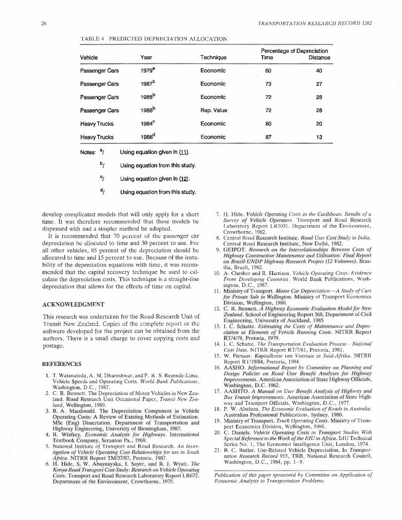
Depreciation was calculated for two scenarios. ln the first, it was assumed that the vehicle was not used over a 12-month period. In the second, it was assumed that the annual utili­zation occurred instantaneously. Comparing these two scenar­ios indicated the allocation between time and distance com­ponents. To allow for comparision, the calculations were performed using the results of the earlier New Zealand studies (11, 12). The resulting allocations are presented in Table 4.

Despite the differences between the 1987 and 1988 passen­ger car predictive relationships, the allocation between the time and distance components remained fairly constant at just over 70 percent due to time and 30 percent to use. This is, however, a substantial change from the 1979 study in which 60 percent of the depreciation was found to be due to time and 40 percent to use. The allocation was found to be similar for both the 1988 replacement value and economic equations.

For medium and heavy commercial vehicles, there has been a similar shift, with the current allocation being approximately 87 percent time and only 13 percent use. This compares with previous values of approximately 80 percent time and 20 per­cent use from the 1984 study. It is recommended that the medium and heavy commercial vehicle allocation be used for light commercial vehicles, buses, and trailers . Although the light commercial vehicle equations did not find utilization significant, a small proportion of the depreciation will undoubtedly arise from vehicle use. This also applies to buses and trailers. Thus , it is recommended that the following values be used for allocating the depreciation costs between time and distance.

Vehicle class

Passenger cars Other vehicle classes

rercentage oj Depreciation Due to

Time

70 85

Distance

30 15

Daniels (20) proposed a technique using knowledge of the vehicle service life and utilization for estimating the allocation of depreciation. This technique was applied by Butler (21) to vehicles in the United States. It is anticipated that future studies will compare the predictions using the method dcvcl­upetl by Daniels (20) with the allocations from the equations developed in this study. This could serve to validate the appli­cability of this latter technique, and allow monitoring of the allocation developed here without having to conduct complicated studies like those undertaken in this project.

CONCLUSIONS

This paper has discussed the depreciation costs of vehicles in New Zealand. Equations were developed for predicting the

Bennell and Dunn 19

TABLE 3 REPORTED ALLOCATIONS OF TIME AND DISTANCE DEPRECIATION COMPONENTS

Country Source Percentage of Depreciation Allocated to Time Distance

U.S.A. AASHO(l.6) 50 50

U.S.A. AASHTO (11) Varies8 Varies8

W. Germany Macdonald (3) 50 50

G. Britain Macdonald (3) 60 40

Denmark Macdonald (3) 0 100

Australia Abelson (la) 60 40

N.Z. MOT (11) 60b 40b

N.Z. MOT (11) 30c 70c

N.Z. Bennett (12) aod 20d

N.Z. MOT (19j 33e 669

Notes: 81 The allocation is a function of utilisation and speed.

For passenger cars.

cl This allocation was used by the Ministry of Works and Development in cost-benefit

studies. It was further assumed that 50 per cent of the distance depreciation was due

to use and 50 per cent to trip related activities.

di For heavy commercial vehicles.

e I For light and heavy commercial vehicles. Various authors cited by (12) also

recommend this split for commercial vehicle depreciation.

rate of depreciation as a function of age and utilization for passenger cars, light commercial vehicles, and medium and heavy commercial vehicles . They were based on data collected from newspapers and the Dealer's Guide.

Two methods were used to calculate the depreciation-the replacement value method and the economic method. The former defines the depreciation as the difference between the cost of a current similar vehicle and the current resale price, while the latter defines the depreciation as the difference between the updated original sales price and the current re­sale price. Only the economic method was used for heavy commercial vehicles. ·

Both techniques were found to yield generally similar results. Thus, it is possible to employ either technique and be con­fident of the results. From an analyst's perspective, the eco­nomic technique is easier and more consistent to employ because it is based on " hard" data available from researching past sales histories. It is difficult to ensure consistency when apply­ing the replacement value method, and the results may be due in large measure to the analyst's judgment.

It is therefore recommended that where necessary, the eco­nomic technique be used in preference to the replacement value technique for calculating the depreciation. In all instances, it was found that age was the dominant effect in motor vehicle depreciation, particularly for light commercial vehicles where the utilization coefficients were not found to be significant.

An investigation was made of the stability of depreciation over time. This was accomplished by performing the same analysis on a data base dating from early 1987 (17 months earlier). It was found that the 1988 depreciation relationship was significantly different from the one developed from the 1987 data. Given the changes in the New Zealand car market that had occurred during this period, some difference was expected, but not of the magnitude observed in this study. When these equations were compared with those from an earlier study conducted in Wellington during 1979, it was again found that the results were significantly different.

Because of the significant differences in the depreciation equations, it appears that the rate of depreciation is not stable over time. As a result , there appears to be little need to

20 TRANSPORTATION RESEARCH RECORD 1262

TABLE 4 PREDICTED DEPRECIATION ALLOCATION

Vehicle Year

Passenger Cars 19798

Passenger Cars 1987b

Passenger Cars 1988b

Passenger Cars 1988b

Heavy Trucks 1984c

Heavy Trucks 1988d

Notes: al Using equation given in (11}.

bl Using equation from this study.

01 Using equation given in (12).

di Using equation from this study.

develop complicated models that will only apply for a short time. It was therefore recommended that these models be dispensed with and a simpler method be adopted.

It is recommended that 70 pe1cenl uf Liu: passenger car depreciation be allocated to time and 30 percent to use. For all other vehicles, 85 percent of the depreciation should be allocated to time and 15 percent to use. Because of the insta­bility of the depreciation equations with time, it was recom­mended that the capital recovery technique be used to cal­culate the depreciation costs. This technique is a straight-line depreciation that allows for the effects of time on capital.

ACKNOWLEDGMENT

This research was undertaken for the Road Research Unit of Tr~nc:it NPnf 7P.-;al".lnrl rri.n~..::i.C' nf tho ~r."""-1""+"" ~a ....... ..-....-+ ..... ,. +\... .... ~ ................... ..._ .,.. •• .__,...,....,. .. ....,. ... .._~, '-''-'.t-'.&VJ ...,..._ L..ll'-' '-''-'.l11f-"1Vl..V .1V}-1V.11. VJ. llJ\,.o

software developed for the project can be obtained from the authors. There is a small charge to cover copying costs and postage.

REFERENCES

1. T . Watanatada , A. M. Dhareshwar, and P. K S. Rezende-Lima. Vehicle peeds and Operating Costs. World Bank Publications, Washington, D.C., 1987.

2. C. R. Bennett. The Depreciation of Motor Vehicles in New Zea­land. Road Research Unit Occasional Paper, Transit New Zea­land, Wellington, 1989.

3. R. A. MacdonRld. The Depreciation omponent in Vehicle Operating Costs: A Review or Existing Methods of Estimation. MSc (Eng) Dissertation. Departmen t or Trnnsportation and Highway Engineering, nive rsity or l3irmingham . 1987 .

4. R . Winfrey. Economic Analysi for Nighwnys. International Textbook ompany, cranton Pa .. 1969.

5. National Institute of Transport and Road Research. An Inves-1igation of Vehicle Operming CO!it Relationships for use in South Africa. NITRR Report TM/37/87, Pretoria , 1987.

6. H. Hide, . W. Abaynayaka , I. Sayer. and R. J . Wyau . The Kenya Roat/ Trnnsporl osr Study: Rlls'e(lrch 011 Vehicle Opemting Cosrs. Transport and Road Rescarcb Laboratory Report LR672_ Department r the nvironmcnt , rowthornc, 1975.

Percentage of Depreciation Technique Time Distance

Economic 60 40

Economic 73 27

Economic 72 28

Rep. Value 72 28

Economic 80 20

Economic 87 13

7. H . Hide. Vehicle Operating Costs in the Caribbean: R .1·1111, of a Survey of Vellicle Oper(llors . Transport and Road Research Laboratory Report LR1031. Department of the Environment, Crowthorne, 1982.

8. Central Road Research Institute. Road User Cos1 S111dy in India. Central Road Research In titutc, New Delhi , 1982.

9. GEil'OT. Research 0 11 1/re /111errelatio11ships Bet111ee11 Costs of Highway '011struc1io11 Mai111e11a11ce a11d Ulitisatio11: Final Repon 011 Brazit-UNDI' liiglrw11y Rese11rclr Project (12 Volumes) . Bras­ilia, Brazil , 1982.

10. A. Chesher and R. Harrison. Vehicle Operating Costs: Evidence From Developing Countries. World Bank Publications, Wash­ington, D .C., 1987.

11. Ministry of Tran. port. Motor Car Depreciation-A Study of Cars for Private Sale in We(lingt<m . Ministry of Transport Economics Divisi.on, Wellington , l\l8U.

12. . R. Dennett. A Highway Eco110111ic Evcd11atio11 Model for New Zealand. ch ol of Engineering Report 36 , Department of ivil E n,:iinecrin,g, University or Auckland. 1985

13. I. . Schutte. E timati11g the OSI of M11i11te11ance and Depre­ciation a £le111e11ts of Vehicle Running Cos/s. NITRR Report RT/4n9, Pretoria, 1979.

14. I. C. Schutte. The Transportation Evaluation Process-National Cost Data. NITRR Report RT/7/81, Pretoria , 1981.

15. W. Pienaar. Kapitalkoste van Voertuie in Suid-Afrika. NITRR Report RT/19/84, Pretoria, 1984.

16. AASHO. l11for11111rio11al Report by 0111111ittee 011 l'/a1111i11g mul Design l'olicies 011 Road User Benefit A11aly ·es for Highway lmprove111e11/s. American Association {State Highway Official , Washington , D. . 1962.

17. AASHTO. A M1111110/ on User Benefit Analysis of flighwny 11ml Bus Transit Improvements. American As ociation or tate High­way and Transport Officials, Washington, D.C., 1977.

18. P. W. Abelson. The Economic Evaluation of Roads in Australia. Australian Profe sio.nal Publications, Sydney, 19 6.

19. Mini try o(Trnnsport. Truck Operating Costs. Ministry of Trans­port Economics Division, Wellington, 1986.

20. C. Daniels. Vt!li icle Operating o IS in Transport Studies With Speci(I/ Reference to the Wo1·k of the EJU i11 Africa. EIU Technical Series No. 1, The Economist Intelligence Unit, London, 1974.

21. B. C. Butle r. Use-Related Vehicle Depreciation. In Transpor­tation R('scarc/1 Record 955 , TRB , utional Research Cow1cil , Washington, D.C., 1984, pp. 1-9.

Publication of this paper sponsored by Committee on Application of Economic Analysis to Transportation Problems.