derivationofconsistenthardrock(1000 < v analysis of kik ... ·...

ORI GINAL RESEARCH PAPER

Derivation of consistent hard rock (1000 < VS < 3000 m/s)GMPEs from surface and down-hole recordings:analysis of KiK-net data

A. Laurendeau1,2 • P.-Y. Bard3 • F. Hollender3,4 •

V. Perron4 • L. Foundotos4 • O.-J. Ktenidou5 •

B. Hernandez1

Received: 15 October 2016 / Accepted: 19 April 2017 / Published online: 2 May 2017� The Author(s) 2017. This article is an open access publication

Abstract A key component in seismic hazard assessment is the estimation of ground motion

for hard rock sites, either for applications to installations built on this site category, or as an

input motion for site response computation. Empirical ground motion prediction equations

(GMPEs) are the traditional basis for estimating ground motion while VS30 is the basis to

account for site conditions. As current GMPEs are poorly constrained for VS30 larger than

1000 m/s, the presently used approach for estimating hazard on hard rock sites consists of

‘‘host-to-target’’ adjustment techniques based on VS30 and j0 values. The present study

investigates alternative methods on the basis of a KiK-net dataset corresponding to stiff and

rocky sites with 500\VS30\ 1350 m/s. The existence of sensor pairs (one at the surface

and one in depth) and the availability of P- and S-wave velocity profiles allow deriving two

‘‘virtual’’ datasets associated to outcropping hard rock sites with VS in the range [1000,

3000] m/s with two independent corrections: 1/down-hole recordings modified from within

The following softwares are employed in this study: 1) the one written by J.-C. Gariel and P.-Y.Bard of the1D reflectivity approach (Kennett 1974); 2) the site_amp v.5.6 program package provided by Dave Boore(U.S. Geological Survey); and the pikwin software developed by Perron et al. (2017).

Electronic supplementary material The online version of this article (doi:10.1007/s10518-017-0142-6)contains supplementary material, which is available to authorized users.

& A. [email protected]

O.-J. [email protected]

1 CEA, DAM, DIF, 91297 Arpajon, France

2 Present Address: Instituto Geofısico Escuela Politecnica Nacional, Quito, Ecuador

3 ISTerre, University of Grenoble Alpes/IFSTTAR, CS 40700, 38058 Grenoble, France

4 CEA, DEN, 13108 St. Paul lez Durance Cedex, France

5 Department of Engineering Science, University of Greenwich, Central Avenue, Chatham Maritime,Kent ME4 4TB, UK

123

Bull Earthquake Eng (2018) 16:2253–2284https://doi.org/10.1007/s10518-017-0142-6

http://orcid.org/0000-0002-5641-2106

http://dx.doi.org/10.1007/s10518-017-0142-6

http://crossmark.crossref.org/dialog/?doi=10.1007/s10518-017-0142-6&domain=pdf

http://crossmark.crossref.org/dialog/?doi=10.1007/s10518-017-0142-6&domain=pdf

https://doi.org/10.1007/s10518-017-0142-6

motion to outcropping motion with a depth correction factor, 2/surface recordings decon-

volved from their specific site response derived through 1D simulation. GMPEs with simple

functional forms are then developed, including a VS30 site term. They lead to consistent and

robust hard-rock motion estimates, which prove to be significantly lower than host-to-target

adjustment predictions. The difference can reach a factor up to 3–4 beyond 5 Hz for very

hard-rock, but decreases for decreasing frequency until vanishing below 2 Hz.

Keywords Hard rock reference motion � Site effects � KiK-net � GMPE � ‘‘Host-to-target’’

adjustments

1 Introduction

Site-specific seismic hazard analysis (SHA) often requires the assessment of regional hazard

for very hard-rock conditions. The presently available methods are all based on the concept

of ‘‘host-to-target’’ adjustment (H2T), with different implementations (e.g., Campbell 2003;

Al Atik et al. 2014) which all imply a number of underlying assumptions. The objective of

the present paper is to investigate some new approaches to develop ground motion pre-

diction equation (GMPE) which be valid for hard rock sites characterized by VS30 -

C 1500 m/s, and to compare their outcomes with more classical H2T approach.

To assess regional seismic hazard in areas of low-to-moderate seismicity (classically called

target region), we typically use GMPEs derived with seismic records from surface stations

located in active seismic areas (host region). These GMPEs are in most cases developed by

mixing different site conditions, with a majority of soil sites (see Ancheta et al. 2014 for the

NGA West 2 database; Akkar et al. 2014 for the RESORCE database). In most GMPEs, the

site is described through a single proxy, the average shear wave velocity over the upper 30 m

(VS30) (e.g., Boore and Atkinson 2008). Several studies have shown the interest to complement

this characterization, at least for rock sites, with their high frequency attenuation properties

(e.g., Silva et al. 1998; Douglas et al. 2010; Edwards et al. 2011; Chandler et al. 2006). The

proxy that is often used in the engineering seismology community to characterize the site-

specific high-frequency content of records is the ‘‘j0’’ value, introduced first by Anderson and

Hough (1984) to represent the attenuation of seismic waves in the first few hundreds of meters

or kilometers beneath the site. Classically, j0 is obtained after a measurement on several tens

of records of the high frequency decay j of the acceleration Fourier amplitude spectrum

(FAS), and investigating its dependence on the epicentral distance R in a log-linear space,

which exhibits a relationship j(r) = j0 ? a�log(R), where the trend coefficient a is related to

the regional Q attenuation effect (Anderson and Hough 1984). The model is described as:

A fð Þ ¼ A0 exp �pj Rð Þf½ � for f [ fE ð1Þ

in which A(f) is FAS, A0 is a source- and propagation-path-dependent amplitude, fE is the

frequency above which the decay is approximately linear, and R is the epicentral distance.

A review of the definition and estimation approaches of j0 is given by Ktenidou et al.

(2014). A rock site can be described with these two proxies, VS30 and j0, for instance in the

stochastic simulation method of Boore (2003). Some recent studies have also shown the

usefulness to include the j0 proxy directly in GMPEs as a complement to VS30 to better

estimate the rock motion (Laurendeau et al. 2013; Bora et al. 2015). The j0 parameter may

also be related, at least partly, to the near-surface attenuation characterized by the S-wave

quality factor QS (or alternatively the damping 1 used in the geotechnical engineering

2254 Bull Earthquake Eng (2018) 16:2253–2284

123

practice, i.e., 1 = 0.5/QS). If the site underground structure (at the scale of a few hundred

meters to a few kilometers) is characterized by a stack of N horizontal layers with different

velocity (VSi, i = 1, N) and damping (QSi) characteristics, the corresponding site-specific

intrinsic attenuation may be integrated along the path of the seismic waves through these N

shallow layers, as indicated by Hough and Anderson (1988):

j0 ¼XN

i¼1

hi

QSiVSi

ð2Þ

In this case, QS considers only the effect of intrinsic attenuation while j0 includes also scat-

tering, especially coming from the soft shallow layers (Ktenidou et al. 2015; Pilz and Fah 2017).

To predict site-specific ground motions (e.g., Rodriguez-Marek et al. 2014; Aristizabal

et al. 2016, 2017), the definition of input motion for site response calculations often

requires the prediction for a hard-rock site (VS30[ 1500 m/s and low j0 values). However,

most of the presently existing GMPEs do not allow such predictions (e.g., Laurendeau

et al. 2013). One solution that was adopted in recent PSHA projects [e.g., Probabilistic

Seismic Hazard Analysis for Swiss Nuclear Power Plant Sites (PEGASOS)] is to adjust

existing GMPEs from the host to the target region, in terms of source, propagation and site

conditions (e.g., Campbell 2003; Cotton et al. 2006). These adjustments require a good

understanding of the mechanisms controlling the ground motion. However, the source

(e.g., stress drop, magnitude scaling) and crustal propagation (e.g., quality factor and its

frequency dependence) terms are not well constrained. In recent projects (e.g., PEGASOS

Refinement Project, Biro and Renault 2012; Thyspunt Nuclear Siting Project, Rodriguez-

Marek et al. 2014), the empirically predicted motion is thus corrected by a theoretical

adjustment factor depending only on two site parameters, VS30 and j0. For example, the

adjustment factor as proposed by Van Houtte et al. (2011) is a ratio of acceleration

response spectra obtained from the point source stochastic simulation method of Boore

(2003). This ratio is computed, for different ranges of magnitude-distance, between a

‘‘standard’’ rock characterized by a VS30 around 800 m/s and j0 typically between 0.02 and

0.05 s (characteristics of the host region), and a ‘‘hard rock’’ characterized by larger VS30

values (from 1500 to over 3000 m/s), and different j0 values, typically lower to much

lower. The two site amplifications are assessed with the quarter wavelength method

(Joyner et al. 1981; Boore 2003) using a family of generic velocity profiles (Boore and

Joyner 1997; Cotton et al. 2006) tuned to VS30 values, and the j0 effect is then added

according to Eq. (1). In such approaches, j0 is most often derived from empirical VS30–j0

relationships established with data coming from different studies in the world (Silva et al.

1998; Douglas et al. 2010; Drouet et al. 2010; Edwards et al. 2011; Chandler et al. 2006;

Van Houtte et al. 2011). The short overview of such relationships presented in Kottke

(2017) indicates typical j0 values around between 0.02 and 0.05 s for standard rock

conditions, and below 0.015 s (and sometimes down to 0.002 s) for hard rock conditions

(VS30 C 1500 m/s). All the corrections are performed in the Fourier domain and then

translated in the response spectrum domain using random vibration theory. This proce-

dure—which is thus implicitly based on rather strong assumptions—allows to obtain rather

smooth rock site amplification functions. Their ratio is the theoretical adjustment factor:

the underlying assumptions indicated above systematically result in a significantly larger

high frequency motion on hard rock site compared to softer, ‘‘standard’’ rock sites, due to

the much lower attenuation (j0 effect supersedes impedance effect). The methodology

proposed by Van Houtte et al. (2011) is actually not the only way to adjust rock ground

motion toward hard-rock motion: Al Atik et al. (2014) propose to estimate the host j0

Bull Earthquake Eng (2018) 16:2253–2284 2255

123

directly from the GMPEs through the inverse random vibration theory (IRVT), while Bora

et al. (2015) estimate directly the host j0 values (though not in the classical way) and

derive a GMPE in the Fourier domain including it. Both approaches thus allow to avoid the

use of VS30–j0 relationships at least for the host region. However, the latter is presently

limited to only one set of data, while the Al Atik et al. (2014) procedure is relatively heavy

as the j0 estimates are scenario dependent. In any case, the comparison recently performed

by Ktenidou and Abrahamson (2016) between the adjustment factors obtained with dif-

ferent analytical methods [named IRVT (Al Atik et al. 2014)] and PSSM (point source

stochastic method, method similar to Van Houtte et al. 2011), show that for similar (VS30,

j0) pairs of values, the IRVT method gives the same tendency for the adjustment factor; in

particular, hard-rock sites with low j0 values should undergo larger amplification at high

frequency. That is why in this study we have chosen to compare our results only with the

PSSM method implemented with the VS30–j0 relationships proposed by Van Houtte et al.

(2011), which can be seen in Kottke (2017) to be a relatively median relation amongst all

the data available by the time the present study was finalized (early 2016). It must be

mentioned however that the latest results by Ktenidou and Abrahamson (2016) on the

NGA-East data conclude at significantly higher than expected j0 values for hard-rock,

eastern NGA sites (typically around 0.02 s), and correlatively smaller motion on hard-rock

sites over the whole frequency range, including the high-frequency range where j0 rela-

tionships are expected to be dominant.

In addition, these host-to-target adjustment factors are associated with large epistemic

uncertainties, which may greatly impact the resulting ground motions estimates especially

for long return periods (e.g., Bommer and Abrahamson 2006). There are mainly three kinds

of uncertainties: those associated with the host region, those associated with the target

region and those associated with the method to define the adjustment factor. Between the

host and the target region, the uncertainties might involve similar issues, addressed

however in different ways for the two regions. Generally, on the host side, the VS-profile

(involving not only VS30, but also its shape down to several kilometers) and j0 are at most

relatively poorly known, or not constrained at all (e.g., when using a generic velocity

profile, or j0 values derived from statistical VS30–j0 correlations, …). On the target side,

site-specific hazard assessment studies generally imply site-specific measurements to

constrain better the velocity profile and sometimes the j0 value; in such cases, there

however exist residual uncertainties associated with the measurement themselves (espe-

cially for j0 values, see for instance Ktenidou and Abrahamson 2016). As a consequence, a

significant source of uncertainties comes from the host GMPE. Indeed, even for a rock with

a VS30 of 800 m/s, the prediction is not well constrained, due to (i) a relative lack of

records for this category (compared to usual, soft and stiff sites) and (ii) a too simplified

site description involving only the VS30 proxy (with often only inferred values) without any

precision on the depth profile. Example of such ‘‘host-GMPE’’ uncertainties may be found

in Laurendeau et al. (2013) who compared soft-rock to hard-rock ratios for different

cases:—empirical ratios from classical, existing GMPEs dependent on only VS30 and

developed with a majority of soil sites;—one deduced from a GMPE dependent on only

VS30 and developed for sites with VS30 C 500 m/s;—theoretical ratios dependent on only

VS30;—and theoretical ratios dependent on VS30 and j0. Finally, two main sources of

methodological uncertainties may be identified in the approaches presently used to esti-

mate the adjustment factors. First, the rock amplification factor associated to the velocity

profile are currently estimated mainly with the impedance, quarter-wavelength approach

(QWL) (Boore and Joyner 1997; Boore 2003), which is not able to reproduce the high-

frequency amplification peaks often observed on measured surface/downhole transfer


123

functions for specific rock sites, and interpreted as related to local resonance effects

(weathering, fracturing, e.g., Steidl et al. 1996; Cadet et al. 2012). Secondly, the need to

move back and forth between Fourier and response spectra through the random vibration

theory (RVT and IRVT, see Al Atik et al. 2014; Bora et al. 2015), also introduces some

additional uncertainties, as this process is strongly non-linear and non-unique.

To get predictions for sites with higher VS30 (C1500 m/s), another possibility is to

employ time-histories recorded at depth. Some GMPEs have been developed from such

recordings, especially those of the KiK-net database, which has sensor pairs (e.g., Cotton

et al. 2008; Rodriguez-Marek et al. 2011). However, these models are not employed in

SHA studies because of the reluctancy of many scientists or engineers to use ‘‘within-

motion’’, depth recordings. In addition to the cost of this installation and heterogeneities

coming from different depths, these records do not represent neither outcropping motion

nor incident motion. They are indeed ‘‘within motion’’ recordings which are affected by

destructive interferences between up-going and down-going waves (e.g., Steidl et al. 1996;

Bonilla et al. 2002). Therefore, the Fourier spectra shape is modified: a trough appears at

the destructive frequency, fdest, which is related to the sensor depth (H) and the mean shear

wave velocity of the upper layers (VM): fdest = VM/4H. The effects of both destructive

interferences and differences of free surface effects have been highlighted by computing

the ratio between surface and depth records both from observations and theoretical linear

SH-1D simulation. This ‘‘outcropping to within motion’’ ratio is around 1 at frequencies

lower than 0.5 fdest; at fdest, a significant peak is observed due to destructive interferences

and finally, at high frequency the ratio is around 1.8 for frequencies exceeding 3 times fdest.

The difference in amplitude between low and high frequencies is related to free surface

effect which is 2 at surface (for quasi-normal incidence) and varying with frequency at the

sensor depth. These effects are observable both in the Fourier and the response spectra

domains. From these observations, Cadet et al. (2012) have proposed a simplified cor-

rection factor for these effects. It was obtained after the analysis of the surface-to-down-

hole ratios derived on the 5% damping pseudo-acceleration spectra. They chose to work in

response spectra domain because its definition implicitly includes a smoothing that limits

the effects of destructive interference at depth.

In this study, a specific subset of the KiK-net dataset, corresponding to stiff sites only

with VS30 C 500 m/s, is used: it is the same as in Laurendeau et al. (2013) and the upper

limit of VS30 values is 1350 m/s. In a first part, the local site-specific site-responses are

estimated with different methods and compared, in order to analyse their reliability in view

of their use for deconvolving the surface recordings into hard rock motion. Secondly,

alternative methodologies to predict the reference motion are explored. These methods

consist in developing GMPEs directly from ‘‘virtual’’ recordings corresponding to

outcropping motion at sites with high S-wave velocity. In other words, the objective is to

apply site-specific corrections (i.e., methods which generally used only for the target site)

to define rock motion in the host region from surface records corrected for the site effects,

or from downhole records corrected of the depth effects. From these datasets, simple

ground motion prediction equations are developed and the results are compared both with

natural data and with classical adjustment method.

1.1 The KiK-net dataset

Japan is in an area of high seismicity, where a lot of high quality digital data are made

available to the scientific community. The KiK-net network (Okada et al. 2004) offers the

advantage of combining pairs of sensors (one at the surface, and one installed at depth in a


123

borehole), together with geotechnical information. Each instrument is a three-component

seismograph with a 24-bit analog-to-digital converter; the KiK-net network uses 200-Hz

(until 27 January 2008) and 100-Hz (since 30 October 2007) sampling frequencies. The

overall frequency response characteristics of the total system is flat, from 0 to 15 Hz, after

which the amplitude starts to decay. The response characteristics are approximately equal

to those of a 3-pole Butterworth filter with a cut-off frequency of 30 Hz (Kinoshita 1998;

Fujiwara et al. 2004). This filter restricts the analysis to frequencies below 30 Hz.

In the present study, we have used the subset of KiK-net accelerometric data previously

built by Laurendeau et al. (2013) consisting basically of crustal events recorded on stiff

sites. More precisely, the selection consisted of the following events and sites:

• Events between April 1999 and December 2009,

• Events described in the F-net catalog and for which MwFnet is larger than 3.5,

• Shallow crustal events with a focal depth less than 25 km were selected and offshore

events were excluded,

• Stiff sites for which in surface VS30 C 500 m/s and at depth VShole C 1000 m/s,

• Surface records with a predicted PGA[ 2.5 cm/s2 using the magnitude-distance filter

by Kanno et al. (2006),

• Records with at least 1 s long pre-event noise,

• Following a visual inspection, faulty records, like S-wave triggers, and records

including multiple events were eliminated or shortened,

• Events and sites with a minimum of three records satisfying the previous conditions.

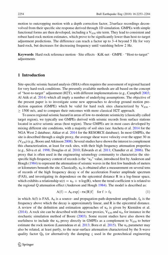
Our dataset finally consists of 2086 six-component records, 272 events and 164 sites

(Table 1). The magnitude-distance distribution is shown on Fig. 1 (left) (see Laurendeau

et al. 2013 for the determination of RRUP). The magnitude range is 3.5–6.9 and the

rupture distance range is 4–290 km. Figure 1 (right) shows the VS distribution of surface

and depth records. In surface, there are no sites with VS30 larger than 1500 m/s, and only

very few (13) sites with VS30 exceeding 1000 m/s. The down-hole sites allow expanding

the distribution until 3000 m/s. The distribution median is around 650 m/s in surface and

around 1900 m/s at depth, and around 1100 m/s when surface and down-hole datasets

are merged.

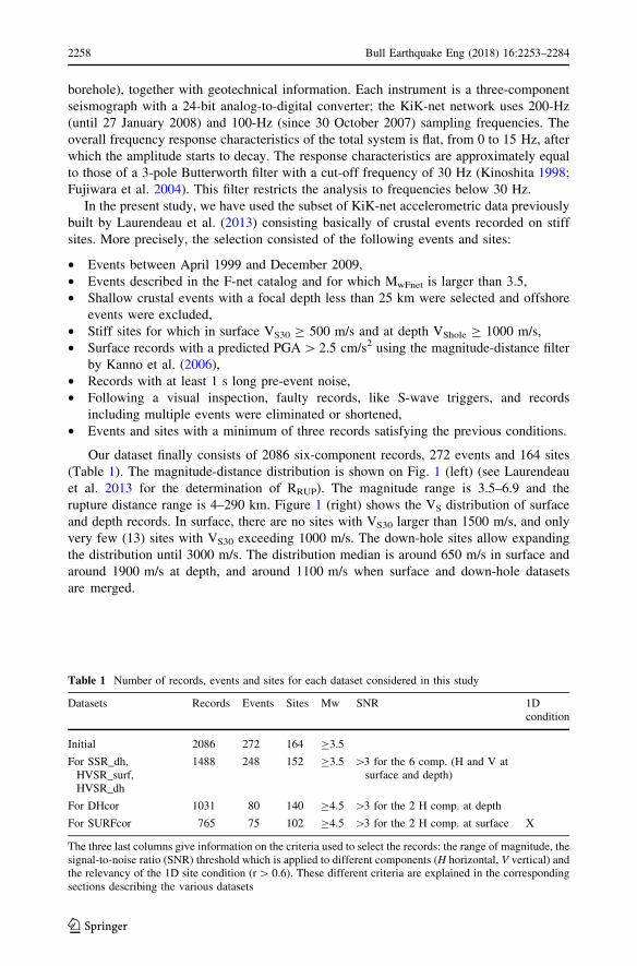
Table 1 Number of records, events and sites for each dataset considered in this study

Datasets Records Events Sites Mw SNR 1Dcondition

Initial 2086 272 164 C3.5

For SSR_dh,HVSR_surf,HVSR_dh

1488 248 152 C3.5 [3 for the 6 comp. (H and V atsurface and depth)

For DHcor 1031 80 140 C4.5 [3 for the 2 H comp. at depth

For SURFcor 765 75 102 C4.5 [3 for the 2 H comp. at surface X

The three last columns give information on the criteria used to select the records: the range of magnitude, thesignal-to-noise ratio (SNR) threshold which is applied to different components (H horizontal, V vertical) andthe relevancy of the 1D site condition (r[ 0.6). These different criteria are explained in the correspondingsections describing the various datasets


123

2 Estimation of the site-specific response

A classical way to estimate site effects consists in using spectral ratios of ground motion

recordings. The horizontal-to-vertical spectral ratios (HVSR) allow only highlighting f0

(under some assumptions) that characterize the resonance frequency in presence of strong

contrasts (e.g., Lermo and Chavez-Garcia 1993). The standard spectral ratios (SSR, ini-

tially proposed by Borcherdt 1970) allow quantifying the amplification (Lebrun et al. 2001)

with respect to the selected reference. The spectral ratios are computed relative to a site

reference chosen either on the surface or on the downhole but near the site, in order that the

characteristics of the incident wave field are similar. The choice of the reference site is a

sensitive issue (e.g., Steidl et al. 1996).

When records are not available, the linear SH-1D simulation can be used to estimate the

theoretical transfer function from the velocity profile. Here, we use the 1D reflectivity

model (Kennett 1974) to derive the response of horizontally stratified layers excited by a

vertically incident SH plane wave (original software written by Gariel and Bard and used

previously in a large number of investigations: e.g., Bard and Gariel 1986; Theodoulidis

and Bard 1995; Cadet et al. 2012). This method requires the knowledge of the shear-wave

velocity profile [VS(z)]. The other geotechnical parameters are deduced from VS(z) using

commonly accepted assumptions, the most critical of which deals with quality factor (QS)

values for each layer.

Without information about VS(z) but with an idea of VS30, the amplification of the site

can be estimated with the quarter wavelength method (QWL) (e.g., Joyner et al. 1981;

Boore 2003) and using generic velocity profiles (Boore and Joyner 1997; Cotton et al.

2006) associated with a VS30 value. This approach is used in most H2T techniques, to

compute the adjustment factor, for instance in Van Houtte et al. (2011). It however relies

on two strong assumptions: (a) VS30 is considered representative of the whole, deep

velocity profile, and (b) the sole impedance effects considered by the QWL method fully

1 10 100

4

5

6

7

RRRUP

(km)

MW

RECORDS: 1488EVENTS: 248SITES: 152

500700 1000 1500 2000 2500 3000 35000

20

40

60

80

VS30(m/s)

snoitats fo rebmu

N

6239

23 278 5

500 1000 1500 2000 2500 3000 35000

20

40

60

80

VShole(m/s)

snoitats fo rebmu

N

17 17 23

31

20 20 21

13

2

Fig. 1 Left distribution of the moment magnitude (MW) and the rupture distance (RRUP) of the preliminaryselection of the KiK-net records (grey dots, see Table 1) and then selected to compute the empirical spectralratios (red dots). The records corresponding to the red dots have a continuous signal-to-noise ratio largerthan 3 between 0.5 and 15 Hz (in this case the signal is the S-wave window). Besides, the empirical spectralratios are computed for each site and event with at least 3 good records. Right VS distribution in terms ofnumber of stations: top in surface and bottom in depth


123

account for the amplification effects on stiff to standard rock sites (in other words, reso-

nance effects are deemed negligible, e.g., Boore 2013).

In this part, the site amplification results obtained from empirical and theoretical

methods will be compared and discussed. Figure 2 displays the different measurements in

a schematic way.

2.1 Computation of the Fourier transfer functions

2.1.1 Standard spectral ratios

For each record, the signal-to-noise ratio (SNR) is estimated both for the vertical com-

ponent and for the 2D complex time-series of the S-wave window of the two orthogonal

horizontal time histories as proposed by Tumarkin and Archuleta (1992). Following

Kishida et al. (2016), the theoretical S-wave window duration (DS) is defined as a function

of source and propagation terms with a minimum duration of 10 s. A noise window is

selected before or after the event with a minimum length of 10 s according to a criterion of

minimal energy. The windowing and the processing are described in detail in Perron et al.

(2017). Each component and window, in surface and at depth, are then processed as

following. A first-order baseline operator is applied to the entire record, in order to have a

zero-mean of the signal, and a simple baseline correction is applied by removing the linear

trend. A 5% cosine taper is applied on each side of the signal window. The records with a

200-Hz sampling frequency are resampled to 100 Hz (to have the same sampling fre-

quency for all the records, without impacting the usable frequency range because of the

built-in low-pass filtering around 30 Hz). The records are padded with zeros in order to

have the same length for all windows (i.e., 8192 samples). We computed FAS for each

component and also for the 2D complex time-series. FAS are smoothed according to the

Konno and Ohmachi (1998) procedure with b = 30. Then, FAS are resampled for a 500

logarithmically spaced sample vector between 0.1 and 50 Hz. Finally, SNR is computed

and the record is selected only if SNR is larger than 3 for a continuous frequency band

between 0.5 and 15 Hz for both the vertical and horizontal components, both in surface and

depth.

Seismic

source

TheoreticalEmpirical

HVSR_surf

HVSR_dh

TF_surf TF_dh

BTFSSR_dh

Fig. 2 Scheme representing the different empirical and theoretical measurements computed to obtain thesite amplification for one site. HVSR is the horizontal-to-vertical spectral ratios (the ‘‘_surf’’ suffix indicatesit is computed at the surface, while the ‘‘_dh’’ suffix stands for the downhole sensor depth), SSR is thestandard spectral ratio (the ‘‘_dh’’ suffix indicates it is computed with respect to a reference at depth), TF isthe numerical transfer function for incident plane S-waves and with respect to outcropping rock (_surfobtained in surface and _dh obtained at the sensor depth), BTF is the associated numerical surface to depthtransfer function (BTF = TF_surf/TF_dh)


123

In addition, the geometrical mean of the three empirical spectral ratios (HVSR_surf,

HVSR_dh, SSR_dh, see Fig. 2) is estimated if there are at least 3 records for the site. With

such selection criteria, the empirical spectral ratios could be finally derived for 152 sites

from 1488 records (Fig. 1; Table 1). The most stringent criterion that eliminates most of

the 2086 - 1488 = 598 recordings is the signal-to-noise threshold.

2.1.2 Linear SH-1D simulation

In addition to the velocity profiles [VP(z) and VS(z)] derived from downhole measure-

ments, the 1D simulation requires to provide the unit mass [q(z)] and damping [QP(z) and

QS(z)] profiles. The Brocher (2005) relationship is used to get q(z) from VP(z). The quality

factors are assumed to be independent of frequency, and inferred from VS(z) according the

following relationships:

QP zð Þ ¼ max VP zð Þ=20; VS zð Þ=5½ � ð3Þ

and

QS zð Þ ¼ VS zð Þ=XQ ð4Þ

in which XQ is a variable, often chosen equal to 10 (e.g., Fukushima et al. 1995; Olsen

et al. 2003; Cadet et al. 2012; Maufroy et al. 2015). Most of the results presented here

(unless specifically indicated) correspond to XQ = 10; however, a sensitivity analysis of

the impact of XQ has been performed to feed the discussion. More details may be found in

Hollender et al. (2015).

The numerical transfer functions (TFs) are computed for 2048 frequency samples

regularly spaced from 0 to 50 Hz, both at the surface (TF_surf), and also at the sensor

depth TF_dh. TF_surf and TF_dh are computed with respect to an outcropping rock. The

Konno and Ohmachi (1998) smoothing is applied with a b coefficient of 10, therefore

lower than in the case of real data but theoretical TFs require a stronger smoothing

especially at depth because of ‘‘pure’’ destructive interferences (see Cadet et al. 2012).

Besides, the theoretical surface to depth transfer function BTF (BTF = TF_surf/TF_dh) is

computed for comparison with the instrumental one SSR_dh.

2.2 Typical site responses

Stiff to ‘‘standard-rock’’ sites present indeed some typical transfer functions which are

illustrated and briefly discussed below to highlight some specific features of their

behaviour.

Figure 3a presents the example of a site with relatively flat transfer functions, such as

what is expected for a reference site, despite the fact this station is characterized by a

relatively low VS30, around 600 m/s. The peak observed on SSR_dh is interpreted as

caused by destructive interferences at depth, since it corresponds to a trough on HVSR_dh

at the same frequency. Would the reference be at the surface, this peak would not exist, as

it is the case for HVSR_surf.

Figure 3b displays an example of a site showing a large amplification, despite the fact

that this site, TCGH14, is characterized by a relatively high VS30, around 850 m/s: this

amplification around 10 Hz is larger than 10. In this case, the destructive interference

effect is more difficult to observe on SSR but clear on HVSR_dh: the large amplitude


123

(around 10) of the peak at 10 Hz combines the actual surface amplification and the absence

of free surface effect at depth for such wavelengths comparable to or smaller than the

sensor depth.

10-1 100 101

Freq. (Hz)

100

101A

mp

lific

atio

n

MYGH06

VS30

593 m/sSSR_DHHVSR_surfHVSR_dh

0 1000 2000 3000V

S (m/s)

0

20

40

60

80

100

Dep

th (

m)

10-1 100 101

Freq. (Hz)

100

101

Am

plif

icat

ion

TCGH14

VS30


0 1000 2000 3000V

S (m/s)

0

20

40

60

80

100

Dep

th (

m)

10-1 100 101

Freq. (Hz)

100

101

Am

plif

icat

ion

NGNH35

VS30


0 1000 2000 3000V

S (m/s)

0

20

40

60

80

100

120

Dep

th (

m)

(a)

(b)

(c)

Fig. 3 Empirical spectral ratios and corresponding S-wave velocity profile for some particular stations.a Example of the site MYGH06 which have a relatively flat transfer functions and with a relatively low VS30

(593 m/s). b Example of the site TCGH14 showing a large amplification at high frequency with a relativelyhigh VS30 (849 m/s). c Example of the site NGNH35 which will be used in the following part as examplebecause it is a well-defined site (VS30 of 512 m/s). The purple patch corresponds to amplification levelsbetween 0.5 and 2 and allows to highlight the amplification. The grey patch corresponds to the frequencyrange for which the signal-to-noise-ratio (0.5–15 Hz) is estimated and is higher than 3


123

Figure 3c shows the example of a well-characterized site (i.e., exhibiting a good cor-

relation coefficient between SSR_dh and BTF), NGNH35 with a VS30 of 512 m/s. Both

HVSR_surf and SSR_dh exhibit a first peak around 3 Hz with an amplitude around 2–3

and 5, respectively. As HVSR_dh exhibits a trough at the same frequency, this first peak is

identified as the fundamental frequency of the site, corresponding to a moderate contrast at

large depth. The transfer functions present a broad and large amplification from 7 to 12 Hz

reaching an amplitude of 16, while the HVSR_surf also exhibits a peak but with a much

more moderate amplitude of 3.5. This high-frequency peak may therefore be interpreted as

due to another impedance contrast at shallow depth.

One may notice that the two NGNH35 and TGCH14 are characterized by a large high-

frequency amplification (exceeding 10 around 10 Hz), despite having quite different VS30

values. Actually, most of the sites in this KiK-net subset exhibit such a high-frequency

amplification (see below).

2.3 Comparison of SSR_dh, BTF and QWL

This part is dedicated to a comparison of the theoretical amplification estimates derived

from 1D site response (resonant type BTF, and impedance effects QWL), with the

observed SSR_dh ratios. After a few examples on some typical sites (Fig. 4), this com-

parison is then performed in a statistical sense on the mean (geometrical average) and

standard deviations (natural log) first for all the sites that are likely to be essentially 1D

(Fig. 5), and finally for various subsets classified according to their VS30 value (Fig. 6).

The downhole-to-surface relative amplification estimate with the QWL approach is

computed by using the actual VS(z) profile and the Dj0 values corresponding to the

cumulative damping effects of each layer from the down-hole sensor to the surface (using

Eq. 2 and QS values estimated with Eq. 4).

Such a comparison is indeed acceptable when the site structure is essentially one-

dimensional, i.e., with quasi-horizontal layers without significant lateral variations.

Thompson et al. (2012) proposed to select 1D sites with reliable velocity profiles by

measuring the fit between SSR_dh and BTF with the Pearson’s correlation coefficient (r).

We implemented the same approach to perform the present statistical comparison: r has

been computed over the frequency range [max(0.5 Hz, 0.5 9 fdest), min(15 Hz, 7 9 fdest)],

in which fdest is the fundamental frequency of destructive interferences at depth, directly

identified on HVSR_dh (see Fig. 3).

Discrepancies between SSR_dh and BTF can have at least two origins: (1) the local site

geometry is not 1D but 2D or 3D, the 1D simulation is no more applicable or (2) the

provided velocity profile of the station is not accurate enough. For Thompson et al. (2012),

sites with r larger than 0.6 are assumed to have 1D-behaviour. Figure 4 shows some

examples of sites with good and bad correlation coefficients. NGNH35 exhibits an

excellent fit between SSR_dh and BTF (r close to 1): BTF predicts the observed ampli-

fication in terms of both frequency range and peak amplitude. The slightly lower r value

(0.77) at KYTH02 is associated to the slight over-prediction of the moderate amplitude

fundamental peak, while the high-frequency, larger amplification (f[ 5 Hz) is very well

matched. On the contrary, MYZH05 and NGSH04 are two examples with very low r

values: BTF does not satisfactorily capture either the amplitude and frequency of the large

amplitude fundamental peak (NGSH04) or the high frequency amplification (MYZH05).

In our dataset as a whole, a total of 108 sites out of 152, i.e., slightly more than two-

thirds, are found to meet the Thompson criterion, i.e., r C 0.6 (see Table 1). In the next


123

sections, the statistical comparison will be limited to these sites. More details on the site

selection and distribution of r values may be found in Hollender et al. (2015).

The statistical comparison displayed in Fig. 5 shows that the average site response of

this whole ‘‘1D subset’’ is far from being flat but exhibits a significant, broadband

amplification around 10 Hz. The mean site responses are relatively similar up to 10 Hz for

SSR_dh and BTF with an amplification around 5–6, while the standard deviation is also

similar and large. It is worth mentioning at this stage that the SSR_dh are in excellent

100 101

Freq. (Hz)

100 Am

plit

ud

e

NGNH35

r: 0.97

VS30

: 512 m/s

100 101

Freq. (Hz)

100 Am

plit

ud

e

MYZH05

r: 0.02

VS30

: 1072 m/s

100 101

Freq. (Hz)

100 Am

plit

ud

e

KYTH02

r: 0.77

VS30

: 518 m/s

100 101

Freq. (Hz)

100 Am

plit

ud

e NGSH04

r: 0.22

VS30

: 633 m/s

SSR_dh + or - 1 SSR_dhBTFTF_surfQWLfrequency range for correlation

Fig. 4 Example comparisons between the instrumental site amplification SSR_dh and the variousnumerical estimates derived from the velocity profile. The sites selected in the left column exhibit a goodSSR_dh/BTF correlation (large r values), while those on the right exhibit a bad correlation (low r values).For the 3 numerical methods (BTF, TF_surf and QWL), QS is defined as QS = VS/10

100 101

Freq. (Hz)

100

101

SSR_dhBTFTF_surfQWL

100 101

Freq. (Hz)

0

0.5

1SSR_dhBTFTF_surfQWL

Fig. 5 Comparison of the mean spectral amplification (left) and the mean standard deviation obtained fromfour different methods for the whole ‘‘1D subset’’ (r C 0.6). For the 3 theoretical methods (BTF, TF_surfand QWL), QS is defined as QS = VS/10


123

agreement with the site terms derived from Generalized Inversion Techniques on the same

data set (see Hollender et al. 2015). Above 15 Hz, the mean amplification is larger in the

case of BTF, which may indicate a bias in the scaling of QS, associated either to an

underestimation of the attenuation (too small XQ) or to the non-consideration of a fre-

quency dependence of QS (note however that frequency–dependent QS models include an

increase of QS with frequency, while here a decrease would be needed—these models are

however derived for deeper crustal propagation, and may not be valid for the shallow depth

considered here).

It is also interesting to compare the associated numerical transfer functions TF_surf with

respect to an outcropping reference, with the amplification curves obtained with the QWL

method, which is the dominant approach used for the velocity adjustment in the H2T

techniques (stochastic modelling based on Boore 2003 approach). As expected, the QWL

estimates cannot account for resonance effects (which are expected even in the case of the

smooth velocity profiles considered in H2T approaches, see for instance Figure 5 in Boore

2013), and are thus steadily increasing with frequency as a consequence of the average

impedance effect at the frequency dependent quarter-wavelength: that is why it does not

reproduce the peak around 10 Hz observed in the transfer function. However, without

considering the peak, the mean amplitude is relatively similar between TF_surf and QWL

(as discussed by Boore 2013). In addition, the same QS scaling than for BTF is used and

again, the amplification level at high frequency is larger than on the observed records. One

must keep in mind however that this apparent overestimation occurs in a frequency range

(beyond 15–20 Hz), where the instrumental results may be biased by the low-pass filtering

100 101

Freq. (Hz)

100

SS

R_d

h

100 101

Freq. (Hz)

100

TF

_su

rf

KiK-net profile

Qs=Vs/10

100 101

Freq. (Hz)

100

BT

F

KiK-net profile

Qs=Vs/10

100 101

Freq. (Hz)

100

QW

LKiK-net profile

0

500 VS30

< 525 m/s (17 sites)

525 VS30

< 575 m/s (25 sites)

575 VS30

< 650 m/s (20 sites)

650 VS30

< 750 m/s (25 sites)

750 VS30

< 900 m/s (14 sites)

900 VS30

< 1500 m/s (7 sites)

Fig. 6 Mean empirical (SSR_dh) and theoretical (BTF) spectral ratios (left) and theoretical transferfunctions (TF_surf and QWL) for different VS30 ranges (see Table 2 for the characteristics of each subset)


123

below 30 Hz implemented in the KiK-net pre-processing of KiK-net data, and that

interpretation of this high frequency difference should thus be performed with due caution.

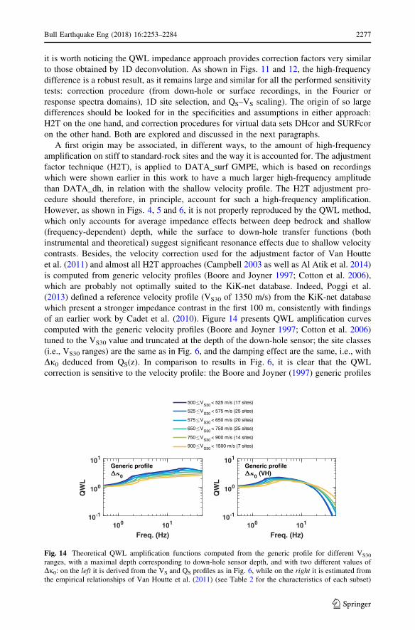
Finally, Fig. 6 provides a comparison of the mean empirical and theoretical spectral

ratios for different VS30 ranges in order to highlight the evolution of site response with

increasing VS30 value. Table 2 presents the characteristics of each VS30 subset, which were

selected to have bins having comparable size: it includes the range of Dj0 values obtained

from the QS and VS profiles (see Eq. 2), which are used for the QWL estimate, together

with the j0 values deduced from the j0–VS30 relationship of Van Houtte et al. (2011).

There are indeed various such relationships in the literature, but this specific one is the

most recent one and includes data of previous studies (Silva et al. 1998; Douglas et al.

2010; Drouet et al. 2010; Edwards et al. 2011; Chandler et al. 2006). Besides, this rela-

tionship is representative of the main tendency exhibited by all other relationships [see for

instance Ktenidou and Abrahamson (2016) or Kottke (2017) for a comparison], except the

one of Edwards et al. (2011), which are associated to significantly lower values. Figure 6

indicates that whatever the approach, the mean spectral ratios are shifted towards higher

frequency when VS30 increases, as expected since the lower velocity layers are thinner and

thinner as VS30 increases. For the 1D estimates BTF and TF_surf, the evolution with VS30

is more regular than for SSR_dh, with a slight trend for the peak amplification to be larger

for the highest VS30. For the VS30 range considered here (i.e., 550–1100 m/s), such a

behaviour is similar to what is predicted by the QWL estimates used in host-to-target

adjustment curves, as they are based on the same velocity and damping profiles. For

example, the theoretical adjustment factor (soft-rock-to-rock ratio), showed in the study of

Laurendeau et al. (2013) for a soft-rock with a VS30 of 550 m/s and a rock with a VS30 of

1100 m/s and computed in the same way than the one of Van Houtte et al. (2011), presents

between 10 and 40 Hz a larger amplification for the rock than for the soft-rock. Around

25 Hz, the theoretical soft-rock-to-rock ratio is around 0.7. On Fig. 6, the ratio between the

first TF_surf curve (VS30 around 525 m/s) and the fifth one (VS30 around 825 m/s) is equal

to 0.77. As to the QWL estimates, the low values of Dj0 associated to the QS scaling result

in very low attenuation effects, so that the amplification curves hardly exhibit some peak

over the considered frequency range (up to 40–50 Hz for the numerical estimates). It must

be emphasized that those Dj0 values are found to be significantly smaller than those found

in the literature as indicated in Table 2 which provides the Dj0 values estimated from the

VS30–j0 relationship of Van Houtte et al. (2011).

Table 2 Characteristics of the various subsets with increasing VS30 range used in Fig. 6 and Fig. 14

VS30

range (m/s)

Number ofsitesincluded

Correspondingrange of VSdh

(m/s)

Dj0

from QS

(ms)

Deduced j0_surf

from VH11(ms)

Deduced j0_dh

from VH11(ms)

Dj0 fromVH11(ms)

500–525 17 1070–2690 1.8–22.6 42.4–44.6 7.5–19.9 23.1–36.5

525–575 25 1100–2780 1.4–5.2 38.5–42.4 7.2–19.3 19.7–34.5

575–650 20 1060–2700 1.2–2.8 33.8–38.5 7.4–20.1 15–28.8

650–750 25 1430–2800 0.9–2.4 29.0–33.8 7.2–14.6 17.8–26.5

750–900 14 1800–3200 0.7–2.1 23.9–29.0 6.2–11.4 16.5–20.4

900–1500 7 1700–2680 0.4–1.1 13.9–23.9 7.5–12.2 6.9–16.3

Only the sites fulfilling the r C 0.6 criterion are selected. The used Dj0 values (the differential attenuationterm between down-hole and surface) as derived from the known VS and assumed QS profiles as indicated inEq. (2) are listed in column 4, and compared to the expected j0_surf–j0_dh difference derived from theVS30–j0 empirical relationships of Van Houtte et al. (2011) (columns 5–7)


123

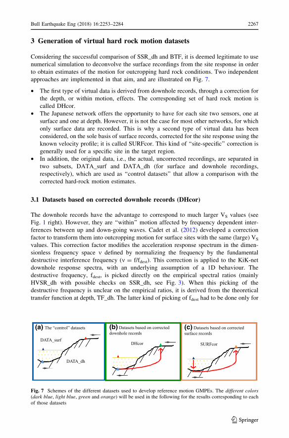
3 Generation of virtual hard rock motion datasets

Considering the successful comparison of SSR_dh and BTF, it is deemed legitimate to use

numerical simulation to deconvolve the surface recordings from the site response in order

to obtain estimates of the motion for outcropping hard rock conditions. Two independent

approaches are implemented in that aim, and are illustrated on Fig. 7.

• The first type of virtual data is derived from downhole records, through a correction for

the depth, or within motion, effects. The corresponding set of hard rock motion is

called DHcor.

• The Japanese network offers the opportunity to have for each site two sensors, one at

surface and one at depth. However, it is not the case for most other networks, for which

only surface data are recorded. This is why a second type of virtual data has been

considered, on the sole basis of surface records, corrected for the site response using the

known velocity profile; it is called SURFcor. This kind of ‘‘site-specific’’ correction is

generally used for a specific site in the target region.

• In addition, the original data, i.e., the actual, uncorrected recordings, are separated in

two subsets, DATA_surf and DATA_dh (for surface and downhole recordings,

respectively), which are used as ‘‘control datasets’’ that allow a comparison with the

corrected hard-rock motion estimates.

3.1 Datasets based on corrected downhole records (DHcor)

The downhole records have the advantage to correspond to much larger VS values (see

Fig. 1 right). However, they are ‘‘within’’ motion affected by frequency dependent inter-

ferences between up and down-going waves. Cadet et al. (2012) developed a correction

factor to transform them into outcropping motion for surface sites with the same (large) VS

values. This correction factor modifies the acceleration response spectrum in the dimen-

sionless frequency space m defined by normalizing the frequency by the fundamental

destructive interference frequency (m = f/fdest). This correction is applied to the KiK-net

downhole response spectra, with an underlying assumption of a 1D behaviour. The

destructive frequency, fdest, is picked directly on the empirical spectral ratios (mainly

HVSR_dh with possible checks on SSR_dh, see Fig. 3). When this picking of the

destructive frequency is unclear on the empirical ratios, it is derived from the theoretical

transfer function at depth, TF_dh. The latter kind of picking of fdest had to be done only for

(c) Datasets based on correctedsurface records

SURFcor

DATA_dh

(a) The “control” datasets

DATA_surfDHcor

(b) Datasets based on correcteddownhole records

Fig. 7 Schemes of the different datasets used to develop reference motion GMPEs. The different colors(dark blue, light blue, green and orange) will be used in the following for the results corresponding to eachof those datasets


123

14 sites, while the former could be achieved directly on empirical ratios for 138 recording

sites.

A total of 1031 records could finally be used to build this first dataset DHcor of

corrected downhole motion and to develop an associated GMPE (see Table 1). For the

original, uncorrected datasets (DATA_dh and DATA_surf), the same collection of events

and sites is used.

3.2 Datasets based on corrected surface records (SURFcor)

Considering that the KiK-net network is the only large network involving pairs of surface

and downhole accelerometers at each site, we tested here another way to derive hard rock

motion directly from the surface records (SURFcor), by using the velocity profiles down to

the downhole sensor to deconvolve the surface motion from the linear site transfer func-

tions with a SH-1D simulation code.

The correction approach (designated as SURFcor) consists in estimating the outcrop-

ping hard rock motion, on the basis of Fourier domain deconvolution. The Fourier

transform of each surface signal is computed and then divided by the SH-1D transfer

function with respect to an outcropping rock consisting of a homogeneous half-space with

a S-wave velocity equal to the velocity at the depth of the down-hole sensor. This esti-

mated outcropping rock spectrum is then converted in time domain by inverse Fourier

transform, and the associated acceleration response spectrum is computed.

To apply such a deconvolution correction, only sites with a probable 1D behaviour (i.e.,

with a correlation coefficient between the empirical and the theoretical ratios larger than

0.6 are selected, as proposed by Thompson et al. (2012). Once again, only the records

associated to a site and an event having recorded at least three records are selected. This

leads to a set of 765 records (see Table 1).

Some variants of this approach were also tested as a sensitivity analysis, in order to

check the robustness of the results (see Laurendeau et al., 2016). Several QS—velocity

scaling were considered, corresponding to XQ values in Eq. (3) ranging from 5 (low

damping) to 50 (large damping), and several incidence angles were also considered, from

0� to 45�. An alternative approach often considered in engineering is to perform the

‘‘deconvolution’’ directly in the response spectrum domain: it was also tested here through

an average ‘‘amplification factor’’ derived from the same 1D simulations for a represen-

tative set of input accelerograms; it is not, however, the recommended procedure as the

response spectrum amplification factor differs for the Fourier transfer function in that it

depends not only on the site characteristics but also on the frequency contents of the

reference motion.

3.3 Direct comparison of the response spectra from the different methods

The different corrections applied to the observed data are based on several assumptions

which allow corrections on a large database. These corrections are not intended to be fully

valid in the case of one particular record, but mainly in a statistical way. However, it is still

interesting to analyse the effect of the corrections for a given record, to highlight their

advantages and disadvantages: Fig. 8 presents a few examples for the three sites already

considered in Fig. 3.

To test the DHcor method, MYGH06 is a relevant site because it is characterized by a

flat SSR_dh (Fig. 3), except at the destructive frequency. A good agreement is observed

between DHcor and DATA_surf (Fig. 8a), providing an indirect check of the depth effect


123

100

101

10−5

10−4

10−3

10−2

10−1

Freq

. (H

z)

) g( AS

MYG

H06

0806

1412

27

Mw

4.9

Rru

p 63

km

Vs30

593

m/s

Vs_h

ole

1480

m/s

100

101

10−5

10−4

10−3

10−2

10−1

Freq

. (H

z)

) g( AS

TCG

H14

0103

3106

09

Mw

5R

rup

36 k

mVs

30 8

49 m

/sVs

_hol

e 23

00 m

/s

100

101

10−5

10−4

10−3

10−2

10−1

Freq

. (H

z)

) g( AS

TCG

H14

0806

1408

43

Mw

6.9

Rru

p 27

0 km

Vs30

849

m/s

Vs_h

ole

2300

m/s

100

101

10−5

10−4

10−3

10−2

10−1

Freq

. (H

z)

) g( AS

NG

NH

3503

0518

0323

Mw

4.6

Rru

p 61

km

Vs30

512

m/s

Vs_h

ole

1500

m/s

100

101

10−5

10−4

10−3

10−2

10−1

Freq

. (H

z)

) g( AS

NG

NH

3504

1025

0605

Mw

5.6

Rru

p 14

6 km

Vs30

512

m/s

Vs_h

ole

1500

m/s

100

101

10−5

10−4

10−3

10−2

10−1

Freq

. (H

z)

) g( AS

NG

NH

3507

0325

0942

Mw

6.7

Rru

p 13

3 km

Vs30

512

m/s

Vs_h

ole

1500

m/s

DAT

A_s

urf

DAT

A_d

hD

Hco

rSU

RFc

or

(a)

(b)

(c)

(d)

(e)

(f)

Fig.8

Com

par

iso

no

fth

ere

spo

nse

spec

tra

for

dif

fere

nt

even

tsre

cord

edat

thre

ed

iffe

ren

tst

atio

ns

ob

tain

edfr

om

the

fou

rd

atas

ets


123

correction factor of Cadet et al. (2012). On the contrary, SURFcor displays slightly lower

amplitudes, probably due to a larger correction factor linked with the shear wave velocity

contrast at shallow depth. In fact, at high frequency the theoretical amplification looks as

insufficiently attenuated for this example. The same behaviour is observed at the same site

for different magnitude-distance scenarios.

The comparison has been also performed for two other example sites characterized by a

SSR_dh with large amplification at high frequency (see Fig. 3). For TCGH14 (Fig. 8b, c),

the site amplification seems insufficiently corrected around the peak for all the scenarios

tested (two are shown here), as SURFcor is larger than DHcor. For NGNH35 (Fig. 8d–f),

the response spectra are relatively similar for the intermediate scenarios. The largest dif-

ferences are observed for the extreme scenarios. The response spectrum of SURFcor

appears insufficiently corrected for the smaller magnitude event, while it appears slightly

over corrected at high frequency for the larger magnitude event. Indeed, it has been shown

repeatedly that the actual site response presents a significant event-to-event variability

(which could be related to incidence or azimuthal angles, as shown in Maufroy et al. 2017),

and the observed variability of the event-to-event differences between SURFcor and

DHcor estimates is certainly linked to such variability, as both SURFcor and the DHcor

corrections are based on average response. However, as will be shown in the next

‘‘GMPE’’ section, the two corrections lead to very similar median predictions, with a larger

variability for the SURFcor approach, which is consistent with the few examples shown

here. One may notice also on these few examples that the corrected spectra are always in-

between the uncorrected surface and down-hole spectra: hard-rock outcropping motion is

found to be (significantly) lower that the stiff or standard-rock motion. The next section is

devoted to investigate to which extent such a result can be generalized and quantified.

4 Comparison in terms of GMPE results

To analyse the overall behaviour of those different real or corrected datasets, we have

chosen to develop ground motion prediction equations based on a simple functional form

in order to get the coefficients directly. Indeed, the functional forms used in the literature

are increasingly complex, requiring fixing some coefficients, which is preformed before-

hand on the basis either of a theoretical simulation or of an empirical analysis of a well-

controlled subset. Given the distribution of our dataset (see Fig. 1), with almost no data in

the near field of large events, and given our focus on the site term, we consider such a

simple functional form to be appropriate for our goal. The ‘‘random effects’’ regression

algorithm of Abrahamson and Youngs (1992) is used to derive GMPEs for the geometrical

mean of the two horizontal components of SA (expressed in g). The following simple

functional form is used:

ln SA Tð Þð Þes¼ a1 Tð Þ þ a2 Tð Þ � MW þ a3 Tð Þ � M2W þ b1 Tð Þ � RRUP� ln RRUPð Þ þ c1 Tð Þ

� ln VS=1000ð Þ þ dBe Tð Þ þ dWes Tð Þ ð5Þ

where dBe is the between-event and dWes the within-event variability, associated with

standard deviations s and u respectively, and rTOT = (s2 ? u2)0.5. VS is either VS30 (for

the control set DATA_surf) or the velocity at down-hole sensor VSDH (for the three other

datasets, real or virtual), which is assumed to be very close of the average velocity over the

30 meters immediate below the down-hole sensor, especially when compared to the high


123

values at depth. That is why, in the following, VS30 is also used for VS values for very hard

rock sites. The resulting coefficients are given in the supplement electronic.

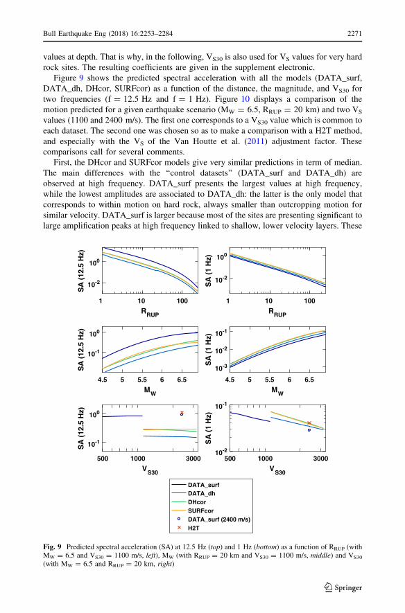
Figure 9 shows the predicted spectral acceleration with all the models (DATA_surf,

DATA_dh, DHcor, SURFcor) as a function of the distance, the magnitude, and VS30 for

two frequencies (f = 12.5 Hz and f = 1 Hz). Figure 10 displays a comparison of the

motion predicted for a given earthquake scenario (MW = 6.5, RRUP = 20 km) and two VS

values (1100 and 2400 m/s). The first one corresponds to a VS30 value which is common to

each dataset. The second one was chosen so as to make a comparison with a H2T method,

and especially with the VS of the Van Houtte et al. (2011) adjustment factor. These

comparisons call for several comments.

First, the DHcor and SURFcor models give very similar predictions in term of median.

The main differences with the ‘‘control datasets’’ (DATA_surf and DATA_dh) are

observed at high frequency. DATA_surf presents the largest values at high frequency,

while the lowest amplitudes are associated to DATA_dh: the latter is the only model that

corresponds to within motion on hard rock, always smaller than outcropping motion for

similar velocity. DATA_surf is larger because most of the sites are presenting significant to

large amplification peaks at high frequency linked to shallow, lower velocity layers. These

1 10 100

RRUP

10-2

100

SA

(12

.5 H

z)

1 10 100

RRUP

10-2

100

SA

(1

Hz)

4.5 5 5.5 6 6.5

MW

10-1

100

SA

(12

.5 H

z)

4.5 5 5.5 6 6.5

MW

10-3

10-2

10-1

SA

(1

Hz)

500 1000 3000

VS30

10-1

100

SA

(12

.5 H

z)

500 1000 3000

VS30

10-2

10-1

SA

(1

Hz)

DATA_surfDATA_dhDHcorSURFcorDATA_surf (2400 m/s)H2T

Fig. 9 Predicted spectral acceleration (SA) at 12.5 Hz (top) and 1 Hz (bottom) as a function of RRUP (withMW = 6.5 and VS30 = 1100 m/s, left), MW (with RRUP = 20 km and VS30 = 1100 m/s, middle) and VS30

(with MW = 6.5 and RRUP = 20 km, right)


123

site effects obviously do not affect DHcor predictions, and are ‘‘statistically’’ removed with

the SURFcor approach.

Between DHcor and SURFcor, small differences are observable mainly at the limits of

the model, i.e., large distances or large magnitudes. The main (though still slight) differ-

ences correspond to the VS30 dependency at high frequency (see Fig. 9). At low frequency,

as expected, the spectral acceleration decreases with increasing VS (the site coefficient c1 is

negative). However, at high frequency, when VS increases, the spectral acceleration stays

almost stable for SURFcor and DATA_surf (the site coefficient c1 is close to zero). This

unexpected observation will be commented later in the Sect. 5, but one may notice that the

same behaviour is observed for the DATA_surf GMPE: this maybe corresponds to the fact

that when the range of VS30 is too small and the actual dependency only weak, there might

be a trade-off between the VS30 dependency (c1 term) and the constant term (a1 term),

leading to the jumps in the c1 coefficient between DATA_surf and the other sets. This led

us to derive other GMPEs by mixing the DATA_surf set with the hard rock sets, in order to

cover a much wider range of VS30 values, as will be discussed later.

Figure 10b also includes an example comparison with typical H2T predictions for a VS

of 2400 m/s, according to the correction factors proposed in Van Houtte et al. (2011). As

indicated in the introduction, this specific H2T implementation has been used here because

it was taking into account the widest set of VS30 and j0 measurements available by the time

we started the present study. The H2T amplitude based on the accepted VS30–j0 rela-

tionship, is found to be 3–4 times larger at high frequency (f[ 10 Hz) compared to DHcor

and SURFcor. The H2T amplitude is obtained after the adjustment of DATA_surf pre-

dictions for a VS30 of 800 m/s, which have also larger amplitude at high frequency than the

other models.

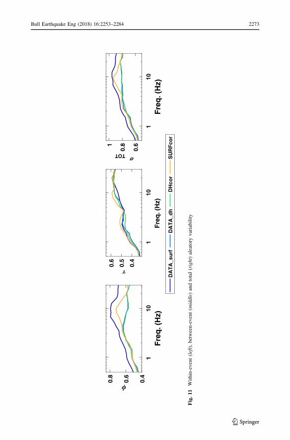
Figure 11 shows the variation of variability with frequency associated with the pre-

dicted spectral accelerations. The total variability (rTOT) associated with the different

datasets is mainly controlled by the within-event variability (u) because the between-event

variability (s) is relatively stable between models. The within-event variability is lower for

the models based on downhole records: DHcor and DATA_dh, indicating that the site to

site variability is significantly lower at depth for a given velocity range. The within-event

variability is larger for the entire range of frequency in the case of DATA_surf. The within-

event variability is larger also around 10 Hz for SURFcor, which corresponds to the

average amplification peak observed for the stiff-soil/soft rock sites considered here.

1 1010

−2

10−1

100

SA

(g

)

Freq. (Hz)

Mw 6.5 Rrup 20km Vs 1100 m/s

DATA_surfDATA_dhDHcorSURFcor

1 1010

−2

10−1

100

SA

(g

)

Freq. (Hz)


DATA_surfDATA_dhDHcorSURFcorH2T

Fig. 10 Comparison of the predicted SA obtained with the empirical models for two VS values and for aspecific scenario MW = 6.5 and RRUP = 20 km. The models are presented with dashed lines when the VS

value is outside the range of VS used to develop the model


123

1 10

Fre

q. (

Hz)

0.6

0.81

TOT

1 10

Fre

q. (

Hz)

0.4

0.5

0.6

1 10

Fre

q. (

Hz)

0.4

0.6

0.8

DA

TA

_su

rfD

AT

A_d

hD

Hco

rS

UR

Fco

r

Fig.11

Wit

hin

-ev

ent

(left)

,bet

wee

n-e

ven

t(m

iddle

)an

dto

tal

(right)

alea

tory

var

iabil

ity


123

5 Discussion

These hard-rock motion prediction results provide the basis for two main types of com-

parisons and discussions, which are presented sequentially in this section: first the inter-

comparison of the two independent correction approaches from down-hole and surface

recordings, and second, as they are very consistent with each other, their comparison with

the hard-rock estimates using the Campbell (2003) H2T approach with Van Houtte et al.

(2011) VS30–j0 relationship.

5.1 Comparison of DHcor and SURFcor predictions

The GMPE comparison highlights a very good agreement between the average predicted

spectral acceleration of DHcor and SURFcor in the case of the tested scenarios (Figs. 9,

10). Although very slight differences may be observed as to their VS30 dependence at high

frequency (see Fig. 9), the main difference between SURFcor and DHcor models lies in the

amount of within-event variability, which is larger for SURFcor at high frequency (see

Fig. 11). Around 10 Hz (the average amplification peak of the stiff sites constituting the

dataset, see Fig. 5), this variability is close to the one of DATA_surf for SURFcor. The

variability associated to SURFcor could be explained by a non-adequate correction of site

effect, linked with inadequate velocity or damping profiles (even though there has been a

tough selection of ‘‘1D’’ sites in the present study).

Firstly, this larger variability on SURFcor could be explained at least partly by the

inadequateness of the 1D correction, even though only the sites with an a priori 1D

behaviour and/or with good parameters to explain the observations [for example, appro-

priate definition of VS(z)] were selected to implement the SURFcor dataset. The selection

criterion as we applied it (r C 0.6) allows to keep a reasonably large number of sites and

recordings (two-thirds, see above). However, in view of applying this correction to other

networks with only surface recordings, empirical spectral ratios are not always available to

constrain the validity of the 1D assumption. That is why a sensitivity test was performed,

with different threshold levels for the r value: without any threshold (i.e., all sites, 1004

records, 79 events and 138 sites), r C 0.6 (704 records, 70 events and 97 sites), r C 0.7

(564 records, 63 events and 76 sites) and r C 0.8 (334 records, 41 events and 45 sites). The

results are displayed on Fig. 12 left for the median estimates for a specific scenario, and on

the right for the corresponding aleatory variabilities. The median estimates are found to

exhibit only a weak sensitivity on the ‘‘1D selection’’, especially when compared with the

difference with H2T estimates. A larger sensitivity is found on the within-event variability,

especially in the high-frequency range (beyond 3.5 and 5 Hz): it is the largest in the case

without any 1D selection and decreases when the selection is more restrictive (higher

correlation coefficient). For the most stringent one (r C 0.8), the within-event variability is

closer to the one found for DHcor. This suggests that the physical relevancy of the pro-

cedure used for the correction of surface records for local site effects is an important

element in reducing the variability associated with hard rock motions. One must however

remain cautious in commenting such results, since the number of available data drops

drastically when the 1D acceptability criterion becomes too stringent.

Secondly, this larger variability on SURFcor could also be partly explained by the

selected QS values used to compute the theoretical site transfer function. In this study, we

have used the standard scaling QS = VS/10 as it is widely used in earthquake engineering

applications (e.g., Fukushima et al. 1995; Olsen et al. 2003; Cadet et al. 2012; Maufroy


123

et al. 2015). However, even if this model allows a satisfactory average fit to the observed

site amplification up to 10 Hz (Fig. 5), it is not the best for all sites and especially, in the

high frequency range. We have thus investigated the sensitivity of the SURFcor correction

to QS by deriving alternative ‘‘SURFcor’’ virtual datasets with different QS–VS scaling.

The results are illustrated in Fig. 13 for the extreme case of very high damping (XQ = 50,

i.e., QS = VS/50). It turns out that the median estimates (shown here for the same scenario)

are not significantly affected by the damping scaling, even at high frequency, while the

within-event variability is found significantly larger at high frequency (f[ 4–5 Hz) for the

larger damping values. An optimal option might be to define for each site the ‘‘best QS

profile’’ in a similar way to what was done by Assimaki et al. (2008), with however the

risk of a significant trade-off between shallow velocity profiles and QS values at

1 10

Freq. (Hz)

10-2

10-1

100

SA

(g

)


SURFcor (all sites)

SURFcor (1D sites >0.6)

SURFcor (1D sites >0.7)SURFcor (1D sites >0.8)H2T

1 10

Freq. (Hz)

0.4

0.6

0.8

1 10

Freq. (Hz)

0.4

0.6

0.8

Fig. 12 Effect of the ‘‘1D’’ selection of sites on predicted SA for SURFcor (left) for a specific scenario(MW = 6.5, RRUP = 20 km) on a hard-rock site (VS = 2400 m/s), and on the within-event u (right top) andbetween-event s (right bottom) variability

1 10

Freq. (Hz)

10-2

10-1

100

SA

(g

)


SURFcor Qs=Vs/10

SURFcor Qs=Vs/50

SURFcor_SA

H2T

1 10

Freq. (Hz)

0.4

0.6

0.8

1 10

Freq. (Hz)

0.4

0.6

0.8

Fig. 13 Sensitivity tests on the SURFcor approach: effects on the median predictions (left) and on thealeatory variability (within-event u, top right; between-event s, bottom right) of the QS–VS scaling and ofthe deconvolution approach (Fourier spectra or response spectra: SA). The considered scenario is the sameas in previous figures: MW = 6.5, RRUP = 20 km, hard-rock with VS = 2400 m/s). Also shown is the H2Tprediction for the same scenario


123

high frequency. Also, it could be possible to consider a frequency-dependent

QS [QS(f) = QS0 9 fa]. Recent investigations on the internal soil damping descriptions

between surface and depth for a few KiK-net sites corresponding EC8 B/C class (E.

Faccioli, personal communication), suggest that Q is linearly increasing with frequency

(a = 1). In our case however, the average results displayed in Fig. 5 for the numerous EC8

A/B sites considered here indicate an overestimation of the mean spectral amplification for

higher frequencies with QS = VS/10. It appears necessary to reduce QS (or to increase XQ)

at high frequency to fit the observations. Such findings might be an indirect indication that

the scaling parameter XQ should be depth dependent with larger values at shallower depth/

or for softer material, which could then be combined with a frequency dependence. In any

case, this also indicates that there is definitely a need for further research on the soil

damping issue, starting with reliable measurement techniques.

Finally and incidentally, we deem it worth mentioning a few words about the ‘‘de-

convolution approach’’ when it is performed in the response spectrum domain through the

use of amplification factors, as often done in the engineering community in relation to site

response, for instance in all GMPEs. It was performed here simply as a sensitivity test to

investigate the potential differences between a correction in Fourier (FSA) and response

spectra (SA) domains. As amplification factors on response spectra are known to be

sensitive to the frequency contents of the input motion, this SA correction was imple-

mented here through an average amplification factor derived for each site from its response

to 15 accelerograms selected in the RESORCE European databank (Akkar et al. 2014) to

cover a wide range of frequency content, with spectral peak varying between 1 and 20 Hz.

More details can be found in Laurendeau et al. (2016). Figure 13 shows that SURF-

cor_FSA and SURFcor_SA result in similar predictions in terms of median response

spectra, with however a much larger high-frequency within-event variability for SURF-

cor_SA. This larger variability is interpreted as due to the highly nonlinear scaling of

response spectra with respect to Fourier spectra computation, especially in the high-fre-

quency range (Bora et al. 2016): the larger variability at high frequency is due to the use of

average amplification factors on response spectra instead of record specific amplification

factors.

5.2 Comparison with the classical H2T approach using the Van Houtte et al.(2011) VS30–j0 relationship

Despite these issues on high frequency variability, the main outcome of this study is to

point out an important difference in the median amplitude of the high frequency motion

predicted by the Van Houtte et al. (2011) H2T approach on the one hand (which has been

repeatedly shown to provide adjustment factors comparable to those obtained with other

H2T methods, see Ktenidou and Abrahamson 2016), and by the different ‘‘hard-rock’’

GMPEs derived here (DHcor and SURFcor) on the other hand. The H2T corrections

applied here are based on the GMPE predictions obtained from surface records

(DATA_surf) for VS30 = 800 m/s, adjusted to a hard rock characterized by a VS around

2400 m/s with the Van Houtte et al. (2011) adjustment factor. The latter is tuned to the j0

values provided by the VS30–j0 relationships derived by the same authors from worldwide

data. This model is compared with the predictions from other datasets only for

VS30 = 2400 m/s (see Figs. 9, 10). For hard rock with velocities beyond 2 km/s, the H2T

estimate is found to be 3–4 times larger at high frequency (f[ 10 Hz) compared to DHcor

and SURFcor, while it decreases with decreasing frequencies, to become negligible at low

frequency (f\ 1 Hz): in the low frequency domain, the key parameter is the velocity, and


123

it is worth noticing the QWL impedance approach provides correction factors very similar

to those obtained by 1D deconvolution. As shown in Figs. 11 and 12, the high-frequency

difference is a robust result, as it remains large and similar for all the performed sensitivity

tests: correction procedure (from down-hole or surface recordings, in the Fourier or

response spectra domains), 1D site selection, and QS–VS scaling). The origin of so large

differences should be looked for in the specificities and assumptions in either approach:

H2T on the one hand, and correction procedures for virtual data sets DHcor and SURFcor

on the other hand. Both are explored and discussed in the next paragraphs.

A first origin may be associated, in different ways, to the amount of high-frequency

amplification on stiff to standard-rock sites and the way it is accounted for. The adjustment

factor technique (H2T), is applied to DATA_surf GMPE, which is based on recordings

which were shown earlier in this work to have a much larger high-frequency amplitude

than DATA_dh, in relation with the shallow velocity profile. The H2T adjustment pro-

cedure should therefore, in principle, account for such a high-frequency amplification.

However, as shown in Figs. 4, 5 and 6, it is not properly reproduced by the QWL method,

which only accounts for average impedance effects between deep bedrock and shallow

(frequency-dependent) depth, while the surface to down-hole transfer functions (both

instrumental and theoretical) suggest significant resonance effects due to shallow velocity

contrasts. Besides, the velocity correction used for the adjustment factor of Van Houtte

et al. (2011) and almost all H2T approaches (Campbell 2003 as well as Al Atik et al. 2014)

is computed from generic velocity profiles (Boore and Joyner 1997; Cotton et al. 2006),

which are probably not optimally suited to the KiK-net database. Indeed, Poggi et al.

(2013) defined a reference velocity profile (VS30 of 1350 m/s) from the KiK-net database

which present a stronger impedance contrast in the first 100 m, consistently with findings

of an earlier work by Cadet et al. (2010). Figure 14 presents QWL amplification curves

computed with the generic velocity profiles (Boore and Joyner 1997; Cotton et al. 2006)

tuned to the VS30 value and truncated at the depth of the down-hole sensor; the site classes

(i.e., VS30 ranges) are the same as in Fig. 6, and the damping effect are the same, i.e., with

Dj0 deduced from QS(z). In comparison to results in Fig. 6, it is clear that the QWL

correction is sensitive to the velocity profile: the Boore and Joyner (1997) generic profiles

100 101

Freq. (Hz)

10-1

100

101

QW

L

Generic profile

0

100 101

Freq. (Hz)

10-1

100

101

QW

L

Generic profile

0 (VH)

500 VS30

< 525 m/s (17 sites)

525 VS30

< 575 m/s (25 sites)

575 VS30

< 650 m/s (20 sites)

650 VS30

< 750 m/s (25 sites)

750 VS30

< 900 m/s (14 sites)

900 VS30

< 1500 m/s (7 sites)

Fig. 14 Theoretical QWL amplification functions computed from the generic profile for different VS30

ranges, with a maximal depth corresponding to down-hole sensor depth, and with two different values ofDj0: on the left it is derived from the VS and QS profiles as in Fig. 6, while on the right it is estimated fromthe empirical relationships of Van Houtte et al. (2011) (see Table 2 for the characteristics of each subset)


123

predict slightly larger and broader frequency amplification (i.e., starting at lower fre-

quency) than the actual KiK-net profiles with their larger velocity gradient at shallow

depth. However, the noticeable difference does not fully explain the large high-frequency

difference between H2T and our approaches, which is also probably related to j0 values, as

discussed in the next section.

Another reason for these high-frequency differences may be related to the site char-

acterization scheme: in the H2T approach, it is based on the twin proxy (VS30, j0), which is

however often reduced to VS30 only through VS30–j0 relationships as those proposed by

Van Houtte et al. (2011) when no site-specific measurement of j0 is available. For the

DHcor set, it is based on the down-hole velocity VSDH and the measured destructive

interference frequency fdest (related to the travel time between the surface and downhole

sensors, i.e., on the surface-downhole average velocity). For the SURFcor sets, it is based

on the full S-wave velocity profile (and the related assumptions on unit mass and damping

profiles). The two latter thus involve more to much more details about the velocity profile,

used before the derivation of GMPEs, while the former (H2T) combines a velocity proxy

and a damping proxy (sometimes simply inferred from the velocity proxy or IRVT), which

are used as a post-correction of GMPE results for ‘‘standard rock’’ sites, on the basis of

stochastic modeling. It is thus not so easy to compare the results obtained in a very

different way. Two items may however be discussed: the site term in the GMPEs, and the

j0 values and their relationship with VS30.

• The site term in SURFcor and DHcor GMPEs is characterized by the coefficient c1

controlling the VS30 dependence. It could indeed implicitly account, at least partially,

for a ‘‘hidden correlation’’ between j0 and VS30. As shown in Fig. 9, c1 is found close

to zero at high frequency, which may reflect some slight decrease of j0 with increasing

VS30.

• This VS30 dependence must however be investigated further, as Fig. 9 indicates a

‘‘step-like’’ difference between DATA_surf (500 B VS B 1000 m/s) and the other

models (1000 B VS B 3000 m/s) for sites having velocities close to their intersection

zone, i.e., around 1000 m/s. For instance, the predicted amplitude is significantly

higher at high frequency (0.84 g for DATA_surf for SA (12.5 Hz) instead of around

0.3 g for the others), and slightly lower at low frequency (0.04 g compared to 0.07 g

for the others). To eliminate the VS gap between the two datasets, a new set of GMPEs

has been derived by mixing the DATA_surf set and the corrected outcropping hard-

rock virtual datasets (DHcor or SURFcor), which allows to explore a much larger VS

range (500 B VS B 3000 m/s). The corresponding results displayed in Fig. 15 replace

the ‘‘jump’’ by a continuous, decreasing dependence on VS, at all frequencies. To

further investigate whether this ‘‘smoothing’’ of the jump is real or imposed by the

‘‘c1�log(VS)’’ functional form, Fig. 16 displays the dependence of within-event

residuals with VS for the ‘‘DATAsurf ? SURFcor’’ case, without (left) and with the

‘‘c1�log(VS)’’ site term (right). The left plot actually supports the existence of the jumps

identified in Figs. 9 and 15, especially at high frequency, while the right plot indicates

the classical functional form performs rather well in reducing the residuals. This

suggests that, even though the correction procedures of downhole or surface recordings

can probably be improved to remove these jumps, there is a definite trend for hard rock

motion to be significantly lower than standard rock motion, even at high frequency.

j0 effects also deserve specific discussion, mainly because the high-frequency increase

of ground motion predicted for very hard-rock sites by the H2T approach is essentially

controlled by j0 values, which are generally assumed to be very low on hard rock sites (see


123

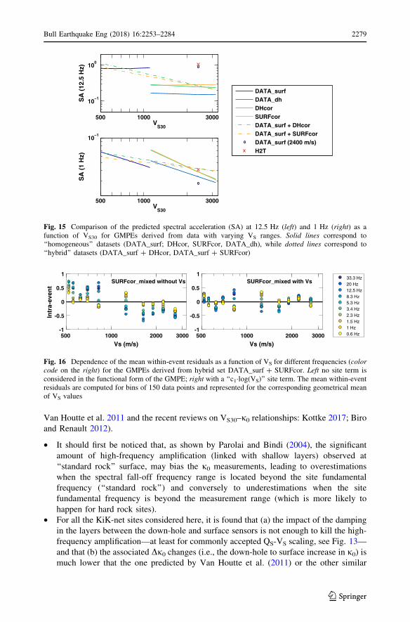
Van Houtte et al. 2011 and the recent reviews on VS30–j0 relationships: Kottke 2017; Biro

and Renault 2012).

• It should first be noticed that, as shown by Parolai and Bindi (2004), the significant

amount of high-frequency amplification (linked with shallow layers) observed at

‘‘standard rock’’ surface, may bias the j0 measurements, leading to overestimations

when the spectral fall-off frequency range is located beyond the site fundamental

frequency (‘‘standard rock’’) and conversely to underestimations when the site

fundamental frequency is beyond the measurement range (which is more likely to

happen for hard rock sites).

• For all the KiK-net sites considered here, it is found that (a) the impact of the damping

in the layers between the down-hole and surface sensors is not enough to kill the high-

frequency amplification—at least for commonly accepted QS-VS scaling, see Fig. 13—

and that (b) the associated Dj0 changes (i.e., the down-hole to surface increase in j0) is

much lower that the one predicted by Van Houtte et al. (2011) or the other similar

500 1000 3000

10−1

100

SA

(12

.5 H

z)

VS30

500 1000 3000

10−1

SA

(1

Hz)

VS30

DATA_surfDATA_dhDHcorSURFcorDATA_surf + DHcorDATA_surf + SURFcorDATA_surf (2400 m/s)H2T

Fig. 15 Comparison of the predicted spectral acceleration (SA) at 12.5 Hz (left) and 1 Hz (right) as afunction of VS30 for GMPEs derived from data with varying VS ranges. Solid lines correspond to‘‘homogeneous’’ datasets (DATA_surf; DHcor, SURFcor, DATA_dh), while dotted lines correspond to‘‘hybrid’’ datasets (DATA_surf ? DHcor, DATA_surf ? SURFcor)

500 1000 2000 3000

Vs (m/s)

-1

-0.5

0

0.5

1

Intr

a-ev

ent

SURFcor_mixed without Vs

500 1000 2000 3000

Vs (m/s)

-1

-0.5

0

0.5

1SURFcor_mixed with Vs

33.3 Hz20 Hz12.5 Hz8.3 Hz5.3 Hz3.4 Hz2.3 Hz1.5 Hz1 Hz0.6 Hz

Fig. 16 Dependence of the mean within-event residuals as a function of VS for different frequencies (colorcode on the right) for the GMPEs derived from hybrid set DATA_surf ? SURFcor. Left no site term isconsidered in the functional form of the GMPE; right with a ‘‘c1�log(VS)’’ site term. The mean within-eventresiduals are computed for bins of 150 data points and represented for the corresponding geometrical meanof VS values


123

VS30–j0 relationships. Even though the values listed in Table 2 correspond to the

median QS scaling, QS = VS/10, the ratio between VH2011 and SURFcor Dj0 values

is around a factor of 10 for every VS30 range. The impact of such a huge difference is

displayed in Fig. 14 which compares the QWL estimates of amplification curves with

both sets of Dj0 values. In other words, a QS scaling around QS = VS/100 (i.e., a QS of

10 for a S-wave velocity of 1000 m/s) would be needed to explain the increase of high-

frequency motion on very hard rock site. Such a scaling seems a priori unlikely.

• Another possibility is that j0 actually corresponds to the effect of damping over a much

larger depth than the one involved in KiK-net sites (mostly 100 and 200 m). This would

however be somewhat inconsistent with the fact that most of the amplification pattern is

well reproduced by the velocity structure over this limited depth, as shown by

Hollender et al. (2015).

Further investigations on the actual values, meaning and impact of j0 are thus definitely

needed, through careful measurements after deconvolution from the high-frequency

amplification effects.

Figure 17 finally summarizes an important outcome of the present study, with the ratios

or predicted ground motion between standard rock (VSH = 800 m/s) and hard-rock

(VST = 2400 m/s) sites, compared with the ratios derived from the classical H2T method

(Campbell 2003) and the VS30–j0 relationship compiled by Van Houtte et al. (2011). When

the VS range lies within the validity range of a given GMPE, such a ratio may be derived

simply from the site term (i.e., the value of c1�log(VST/VSH): this is possible only for the 2

hybrid GMPEs (DATA_surf ? SURFcor) and (DATA_surf ? DHcor). The ratio was also

computed for a given scenario event (MW = 6.5, RRUP = 20 km) from the response

spectra estimated with different GMPEs (i.e., DATA_surf for standard rock, and SURFcor

or DHcor for hard rock). As can be expected from the previous comparisons and sensitivity

101

Freq. (Hz)

0

0.5

1

1.5

2

2.5

3

R-t

o-H

R r

atio

s

R-to-HR : 800 / 2400

VH2011 adjustment factor median

DATA_surf(800m/s) / DHcor(2400m/s)

DATA_surf(800m/s) / SURFcor(2400m/s)DHcor_mixed(800m/s) / DHcor_mixed(2400m/s)

SURFcor_mixed(800m/s) / SURFcor_mixed(2400m/s)

Fig. 17 Comparison of the ratios between standard rock (VS = 800 m/s) and hard-rock (VS = 2400 m/s)obtained with the GMPEs derived in the present work (dashed lines), and those predicted with the H2Tapproach and the VS30–j0 approach of Van Houtte et al. (2011). The specific scenario considered here is(MW = 6.5; RRUP = 20 km), but the ratios obtained with the hybrid GMPEs (DATA_surf ? SURFcor andDATA_surf ? DHcor) are the same whatever the scenario


123

tests, the results are very consistent for all the GMPEs, with a significant high frequency

reduction on hard rock (basically a factor 2.5–3), corresponding to the high frequency

resonant amplification consistently observed at the surface of all stiff and ‘‘standard-rock’’

sites. On the opposite, the classical Campbell (2003) H2T approach coupled with the VS30–

j0 relationship compiled by Van Houtte et al. (2011), predicts a high frequency increase on

hard-rock (by a factor about 1.25 at 10 Hz and 2 at 30 Hz), resulting from the assumed

much lower j0 values on very-hard rock. These large, high-frequency differences decrease

progressively with decreasing frequency, to completely vanish for frequencies below 2 Hz,

where all approaches predict a slightly larger motion on ‘‘standard rock’’ (around 20–30%).

Though obtained with a completely different approach, the present results prove qualita-

tively consistent with the recent findings by Ktenidou and Abrahamson (2016), who

analyzed a large data set including NGA-east data and others from sites with VS30 -

C 1500 m/s, and conclude at smaller motion on hard-rock (compared to standard rock)

over the whole frequency range. It must be noticed however that their ratios are closer to

unity than ours, and that only few of the hard-rock sites they consider have actually

measured VS30 values, while in our case we have the VS profile but do not have j0 values.

Significant forward steps would come from datasets with many hard-rock sites with

carefully measured VS30 and j0 values.

6 Conclusion

The purpose of this study was to improve the understanding and the estimation of ground

motion from very hard rock sites (1000 B VS B 3000 m/s) through an original processing

of a subset of Japanese KiK-net recordings corresponding to stiff soils and standard rock.

Firstly, the analysis of the Japanese local site-specific responses shows that the sites

with a relatively high VS30 (500\VS30\ 1350 m/s) are characterized by a significant

high-frequency amplification of about 4–5 around 10 Hz in average.

Secondly, the pairs of recordings at surface and depth, together with the knowledge of

the velocity profile, allow to derive different sets of ‘‘virtual’’ outcropping, hard-rock

motion data corresponding to sites with velocities in the range [1000–3000 m/s]. The

corrections are based either on a transformation of deep, within-motion to outcropping

motion (DHcor), or on a deconvolution of surface recordings using the velocity profile and

1D simulation (SURFcor). Each of these virtual ‘‘outcropping hard-rock motion’’ data sets

is then used to derive GMPEs with simple functional forms, using as site condition proxy

the S-wave velocity at depth (VSDH). The predicted response spectra are finally compared

with those obtained with the classical ‘‘hybrid empirical’’ host-to-target adjustment (H2T)

approach initially proposed by Campbell (2003), coupled with the VS30–j0 relationship

compiled by Van Houtte et al. (2011). This comparison exhibits strong differences for short

periods, where the H2T approach leads to predictions 3–4 times larger than the new

approach presented here, in the case of hard-rock sites with VS30 around 2400 m/s, and a

predicted j0 value around 8 ms. Those differences decrease with increasing period, to

completely vanish for periods exceeding 0.5 s.

The original data set (KiK-net recordings from stiff sites with VS30 C 500 m/s,

1999–2009 only) is limited and has considerably enlarged over recent years. The present

results should thus be considered as a first step and should be updated with an enriched

dataset. However, the consistency between results obtained with completely independent

correction methods (SURFcor and DHcor) allows to highlight the possible existence of a


123

significant bias in the classical H2T method coupled with the usually accepted VS30–j0

relationship, which lead to an overestimation of the hard-rock motion possibly reaching

factors up to 3–4 at high frequency (f[ 10 Hz). Our interpretation of this bias is related to

the existence of a significant, high-frequency amplification on stiff soils and standard

rocks, due to thin, shallow, medium velocity layers. Not only this resonant-type amplifi-

cation is not correctly accounted for by the quarter-wavelength approach used for the VS

correction factor used in the all H2T adjustment techniques, but it may also significantly

impact and bias the j measurements, and as a consequence the (VS30–j0) relationships

implicitly used in H2T techniques.

The approaches proposed here might be applied to other strong motion datasets, pro-

vided the velocity profile is known at each recording site in order to deconvolve from the

site-specific effects. This emphasizes once again the high added value of rich site metadata

in all strong motion databases.

Acknowledgements We thank Ezio Faccioli and Philippe Renault for their help to improve the originalpaper. This work was carried out under the SINAPS@ project that receives French funding managed by theNational Research Agency under the program ‘‘Future Investments’’ (Sinaps@ reference: ANR-11-RSNR-0022). Sinaps@ is a ‘‘Seism Institute’’ project (http://www.institut-seism.fr/en/). This work also benefitsfrom previous works carried out within the frameworks of the CASHIMA program (funded by CEA, ILLand ITER) and the SIGMA program (funded by EdF, CEA, Areva and Enel). We are indebted to theNational Research Institute for Earth Science and Disaster Prevention (NIED), Japan, for providing the KiK-net data and the F-NET information used for this analysis.

Open Access This article is distributed under the terms of the Creative Commons Attribution 4.0 Inter-national License (http://creativecommons.org/licenses/by/4.0/), which permits unrestricted use, distribution,and reproduction in any medium, provided you give appropriate credit to the original author(s) and thesource, provide a link to the Creative Commons license, and indicate if changes were made.

References

Abrahamson N, Youngs R (1992) A stable algorithm for regression analyses using the random effectsmodel. Bull Seismol Soc Am 82(1):505–510

Akkar S, Sandıkkaya MA, Senyurt M, Sisi AA, Ay BO, Traversa P et al (2014) Reference database forseismic ground-motion in Europe (RESORCE). Bull Earthq Eng 12(1):311–339

Al Atik L, Kottke A, Abrahamson N, Hollenback J (2014) Kappa (j) scaling of ground-motion predictionequations using an inverse random vibration theory approach. Bull Seismol Soc Am 104(1):336–346

Ancheta TD, Darragh RB, Stewart JP, Seyhan E, Silva WJ, Chiou BSJ, Wooddel KE, Graves RW, KottkeAR, Boore DM, Kishida T, Donahue JL (2014) NGA-West2 database. Earthq Spectra 30(3):989–1005

Anderson J, Hough S (1984) A model for the shape of the Fourier amplitude spectrum of acceleration at highfrequencies. Bull Seismol Soc Am 74:1969–1993

Aristizabal C, Bard P-Y, Beauval C, Lorito S, Selva J et al (2016) Guidelines and case studies of sitemonitoring to reduce the uncertainties affecting site-specific earthquake hazard assessment. Deliver-able D3.4—STREST—harmonized approach to stress tests for critical infrastructures against naturalhazards. http://www.strest-eu.org/opencms/opencms/results/. 2016. Web. 25 April 2016

Aristizabal C, Bard P-Y, Beauval C (2017) Site-specific psha: combined effects of single station sigma,host-to-target adjustments and non-linear behavior. In: 16WCEE 2017 (16th world conference onearthquake engineering, Santiago Chile, January 9–13, 2017), paper # 1504

Assimaki D, Li W, Steidl JH, Tsuda K (2008) Site amplification and attenuation via downhole arrayseismogram inversion: a comparative study of the 2003 Miyagi-Oki aftershock sequence. Bull SeismolSoc Am 98(1):301–330

Bard P-Y, Gariel J-C (1986) The seismic response of two-dimensional sedimentary deposits with largevertical velocity gradients. Bull Seismol Soc Am 76(2):343–346

Biro Y, Renault P (2012) Importance and impact of host-to-target conversions for ground motion predictionequations in PSHA. In: 15 WCEE, Lisboa


123

http://www.institut-seism.fr/en/

http://creativecommons.org/licenses/by/4.0/

http://www.strest-eu.org/opencms/opencms/results/

Bommer JJ, Abrahamson NA (2006) Why do modern probabilistic seismic-hazard analyses often lead toincreased hazard estimates? Bull Seismol Soc Am 96(6):1967–1977

Bonilla LF, Steidl JH, Gariel JC, Archuleta RJ (2002) Borehole response studies at the Garner Valleydownhole array, southern California. Bull Seismol Soc Am 92(8):3165–3179

Boore D (2003) Simulation of ground motion using the stochastic method. Pure Appl Geophys 160:635–676Boore DM (2013) The uses and limitations of the square-root-impedance method for computing site

amplification. Bull Seismol Soc Am 103(4):2356–2368Boore DM, Atkinson GM (2008) Ground-motion prediction equations for the average horizontal component

of PGA, PGV, and 5%-damped PSA at spectral periods between 0.1 s and 10.0 s. Earthq Spectra24(1):99–138

Boore D, Joyner W (1997) Site amplifications for generic rock sites. Bull Seismol Soc Am 87:327–341Bora SS, Scherbaum F, Kuehn N, Stafford P, Edwards B (2015) Development of a response spectral ground-

motion prediction equation (GMPE) for seismic-hazard analysis from empirical fourier spectral andduration models. Bull Seismol Soc Am 105(4):2192–2218

Bora SS, Scherbaum F, Kuehn N, Stafford P (2016) On the relationship between Fourier and responsespectra: implications for the adjustment of empirical ground-motion prediction equations (GMPEs).Bull Seismol Soc Am 106(3):1235–1253

Borcherdt RD (1970) Effect on local geology on ground motion near San Francisco bay. Bull Seismol SocAm 60:29–61

Brocher TM (2005) Empirical relations between elastic wavespeeds and density in the earth’s crust. BullSeismol Soc Am 95(6):2081–2092

Cadet H, Bard P-Y, Rodriguez-Marek A (2010) Defining a standard rock: propositions based on the KiK-netdata. Bull Seism Soc Am 100(1):172–195. doi:10.1785/0120090078

Cadet H, Bard P-Y, Rodriguez-Marek A (2012) Site effect assessment using KiK-net data: part 1. A simplecorrection procedure for surface/downhole spectral ratios. Bull Earthq Eng 10(2):421–448

Campbell KW (2003) Prediction of strong ground motion using the hybrid empirical method and its use inthe development of ground-motion (attenuation) relations in eastern North America. Bull Seismol SocAm 93(3):1012–1033

Chandler AM, Lam NTK, Tsang HH (2006) Near-surface attenuation modelling based on rock shear-wavevelocity profile. Soil Dyn Earthq Eng 26:1004–1014

Cotton F, Scherbaum F, Bommer J, Bungum H (2006) Criteria for selecting and adjusting ground-motionmodels for specific target regions: application to central Europe and rock sites. J Seismol 10:137–156

Cotton F, Pousse G, Bonilla F, Scherbaum F (2008) On the discrepancy of recent European ground-motionobservations and predictions from empirical models: analysis of KiK-net accelerometric data andpoint-sources stochastic simulations. Bull Seismol Soc Am 98(5):2244

Douglas J, Gehl P, Bonilla LF, Gelis C (2010) A j model for mainland France. Pure Appl Geophys167(11):1303–1315

Drouet S, Cotton F, Gueguen P (2010) VS30, j, regional attenuation and Mw from accelerograms: appli-cation to magnitude 3–5 French earthquakes. Geophys J Int 182(2):880–898

Edwards B, Faeh D, Giardini D (2011) Attenuation of seismic shear-wave energy in Switzerland. Geophys JInt 185:967–984

Fujiwara H, Aoi S, Kunugi T, Adachi S (2004) Strong-motion observations of NIED: K-NET and KiK-net.In: Proceedings of the COSMOS workshop on record processing guidelines

Fukushima Y, Gariel JC, Tanaka R (1995) Site-dependent attenuation relations of seismic motion param-eters at depth using borehole data. Bull Seismol Soc Am 85(6):1790–1804

Hollender F, Foundotos L, Laurendeau A, Bard P-Y, Hernandez B, Drouet S, Ktenidou OJ, Perron V, LetortJ (2015) Correction of surface records of their site effect before developing GMPE: an alternativeapproach to get reference incident ground motion (application to KiK-net data). In: SIGMA/SINAPS@report ref. SINAPS@-2015-V1-A1-T3-1, June 2015

Hough SE, Anderson JG (1988) High-frequency spectra observed at Anza, California: implications for Qstructure. Bull Seismol Soc Am 78:692–707

Joyner WB, Warrick RE, Fumal TE (1981) The effect of Quaternary alluvium on strong ground motion inthe Coyote Lake, California, earthquake of 1979. Bull Seismol Soc Am 71(4):1333–1349

Kanno T, Narita A, Morikawa N, Fujiwara H, Fukushima Y (2006) A new attenuation relation for strongground motion in Japan based on recorded data. Bull Seismol Soc Am 96(3):879–897

Kennett BLN (1974) Reflections, rays, and reverberations. Bull Seismol Soc Am 64(6):1685–1696Kinoshita S (1998) Kyoshin net (K-NET). Seismol Res Lett 69(4):309–332Kishida T, Ktenidou OJ, Darragh RB, Walter S (2016) Semi-automated procedure for windowing time series

and computing Fourier amplitude spectra (FAS) for the NGA-West2 database. PEER report no.2016/02


123

http://dx.doi.org/10.1785/0120090078

Konno K, Ohmachi T (1998) Ground-motion characteristics estimated from spectral ratio between hori-zontal and vertical components of microtremor. Bull Seismol Soc Am 88(1):228–241

Kottke AR (2017) VS30–j0 relationship implied by ground motion models? In: 16WCEE 2017 (16th worldconference on earthquake engineering, Santiago Chile, January 9–13, 2017), paper # 3089

Ktenidou OJ, Abrahamson NA (2016) Empirical estimation of high-frequency ground motion on hard rock.Seismol Res Lett 87(6):1465–1478

Ktenidou O-J, Cotton F, Abrahamson NA, Anderson JG (2014) Taxonomy of j: a review of definitions andestimation approaches targeted to applications. Seismol Res Lett 85:135–146

Ktenidou OJ, Abrahamson NA, Drouet S, Cotton F (2015) Understanding the physics of kappa (j): insightsfrom a downhole array. Geophys J Int 203(1):678–691

Laurendeau A, Cotton F, Ktenidou O-J, Bonilla L-F, Hollender F (2013) Rock and stiff-soil site amplifi-cation: dependency on VS30 and kappa (j0). Bull Seismol Soc Am 103(6):3131–3148

Laurendeau A, Bard P-Y, Hollender F, Ktedinou OJ, Foundotos L, Hernandez B, Perron V (2016) Predictionof reference motions (1000\Vs\ 3000 m/s) from corrected KiK-net records of the local site effects.In: 5th IASPEI/IAEE international symposium: effects of surface geology on seismic motion, August15–17, Taipei

Lebrun B, Hatzfeld D, Bard P-Y (2001) A site effect study in urban area: experimental results in Grenoble(France). Pure Appl Geophys 158:2543–2557

Lermo J, Chavez-Garcia FJ (1993) Site effect evaluation using spectral ratios with only one station. BullSeismol Soc Am 83(5):1574–1594

Maufroy E, Chaljub E, Hollender F, Kristek J, Moczo P, Klin P, De Martin F (2015) Earthquake groundmotion in the Mygdonian Basin, Greece: the E2VP verification and validation of 3D numerical sim-ulation up to 4 Hz. Bull Seismol Soc Am 105:1398–1418. doi:10.1785/0120140228

Maufroy E, Chaljub E, Theodoulidis N, Roumelioti Z, Hollender F, Bard P-Y, De Martin F, Guyonnet-Benaize C, Margerin L (2017) Source-related variability of site response in the Mygdonian basin(Greece) from accelerometric recordings and 3-D numerical simulations. BSSA. doi:10.1785/0120160107

Okada Y, Kasahara K, Hori S, Obara K, Sekiguchi S, Fujiwara H, Yamamoto A (2004) Recent progress ofseismic observation networks in Japan—Hi-net, F-net, K-NET and KiK-net. Earth Planets Space56:xv–xxviii

Olsen K, Day S, Bradley C (2003) Estimation of Q for long-period ([2 sec) waves in the Los Angeles basin.Bull Seismol Soc Am 93:627–638

Parolai S, Bindi D (2004) Influence of soil-layer properties on k evaluation. Bull Seismol Soc Am94(1):349–356

Perron V, Laurendeau A, Hollender F, Bard P-Y, Gelis C, Traversa P (2017) Selecting time windows ofseismic phases and noise for engineering seismology applications: a versatile methodology andalgorithm. Bull Earthq Eng. doi:10.1007/s10518-017-0131-9

Pilz M, Fah D (2017) The contribution of scattering to near-surface attenuation. J Seismol 1–19. doi:10.1007/s10950-017-9638-4

Poggi V, Edwards B, Fah D (2013) Reference S-wave velocity profile and attenuation models for ground-motion prediction equations: application to Japan. Bull Seismol Soc Am 103(5):2645–2656

Rodriguez-Marek A, Montalva GA, Cotton F, Bonilla F (2011) Analysis of single-station standard deviationusing the KiK-net data. Bull Seismol Soc Am 101(3):1242–1258

Rodriguez-Marek A, Rathje EM, Bommer JJ, Scherbaum F, Stafford PJ (2014) Application of single-stationsigma and site-response characterization in a probabilistic seismic-hazard analysis for a new nuclearsite. Bull Seismol Soc Am 104:1601–1619

Silva W, Darragh RB, Gregor N, Martin G, Abrahamson N, Kircher C (1998) Reassessment of site coef-ficients and near-fault factors for building code provisions. Technical report program element II:98-HQ-GR-1010, Pacific Engineering and Analysis, El Cerrito

Steidl JH, Tumarkin AG, Archuleta RJ (1996) What is a reference site? Bull Seismol Soc Am86(6):1733–1748

Theodoulidis N, Bard P-Y (1995) Horizontal to vertical spectral ratio and geological conditions—ananalysis of strong ground motion data from Greece and Taiwan (smart-1). Soil Dyn Earthq Eng14(3):177–197

Thompson EM, Baise LG, Tanaka Y, Kayen RE (2012) A taxonomy of site response complexity. Soil DynEarthq Eng 41:32–43

Tumarkin AG, Archuleta RJ (1992) Parametric models of spectra for ground motion prediction. Seismol ResLett 69:30

Van Houtte C, Drouet S, Cotton F (2011) Analysis of the origins of j (kappa) to compute hard rock to rockadjustment factors for GMPEs. Bull Seismol Soc Am 101(6):2926–2941


123

http://dx.doi.org/10.1785/0120140228

http://dx.doi.org/10.1785/0120160107

http://dx.doi.org/10.1785/0120160107

http://dx.doi.org/10.1007/s10518-017-0131-9

http://dx.doi.org/10.1007/s10950-017-9638-4

http://dx.doi.org/10.1007/s10950-017-9638-4

derivationofconsistenthardrock(1000 < v analysis of kik ... ·...

Documents