descriptive statistics a.a. elimam college of business san francisco state university

Descriptive Statistics

A.A. Elimam

College of Business

San Francisco State University

Statistics

The Science of collecting, organizing, analyzing, interpreting and presenting data

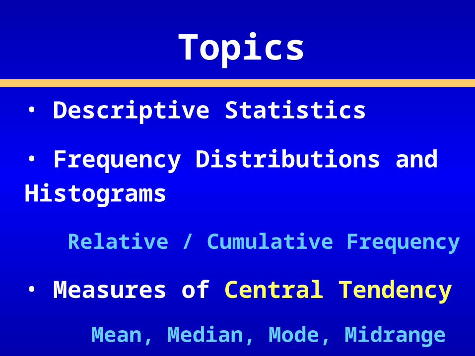
Topics

• Descriptive Statistics

• Frequency Distributions and Histograms

Relative / Cumulative Frequency

• Measures of Central Tendency

Mean, Median, Mode, Midrange

Topics

• Measures of Dispersion (Variation) Range, Standard Deviation, Variance and Coefficient of variation• Shape Symmetric, Skewed, using Box-and- Whisker Plots• Quartile• Statistical Relationships Correlation , Covariance

A collection of quantitative measures and

ways of describing data. This includes:

Frequency distributions & histograms, measures of central tendency

and

measures of dispersion



•Collect Data e.g. Survey

•Present Data e.g. Tables and Graphs

•Characterize Data e.g. Mean

nx i

A Characteristic of a: Population is a Parameter

Sample is a Statistic.

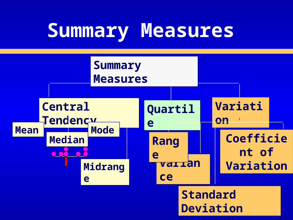
Summary Measures

Central Tendency

MeanMedian

Mode

Midrange

Quartile

Summary Measures

Variation

Variance

Standard Deviation

Coefficient of Variation

Range

Measures of Central Tendency

Central Tendency

Mean Median Mode

Midrangen

xn

ii

1

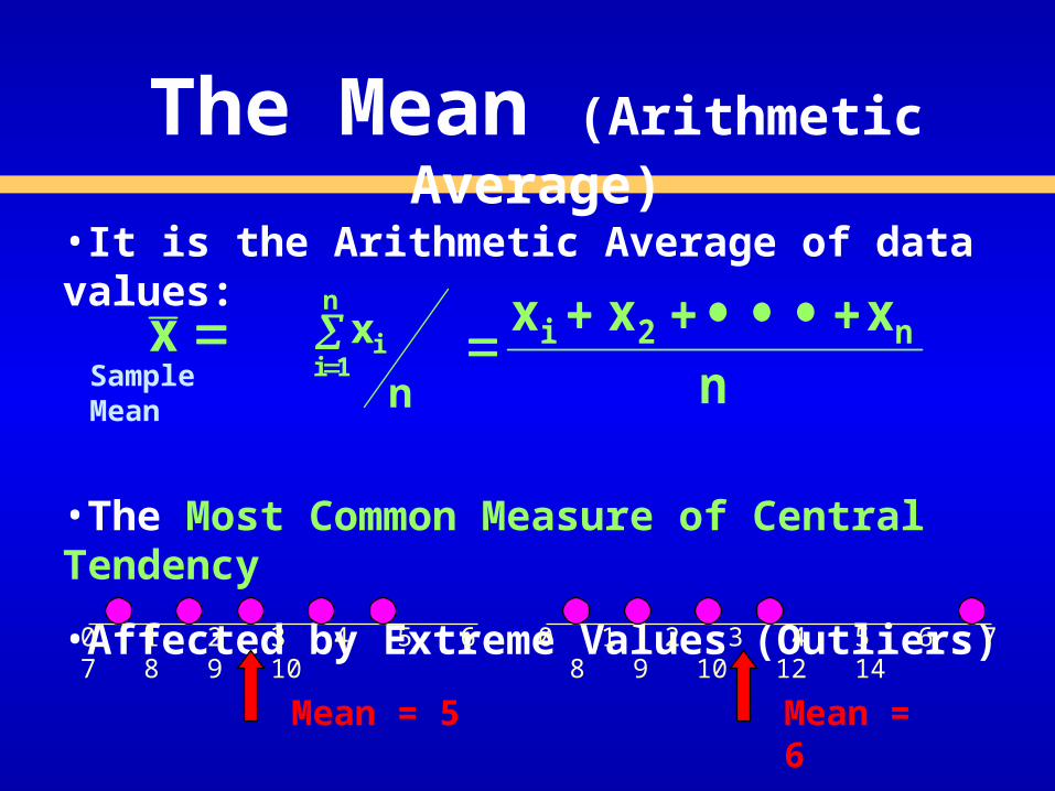
The Mean (Arithmetic Average)

•It is the Arithmetic Average of data values:

•The Most Common Measure of Central Tendency

•Affected by Extreme Values (Outliers)

n

xn

1ii

n

xxx n2i

0 1 2 3 4 5 6 7 8 9 10 0 1 2 3 4 5 6 7 8 9 10 12 14

Mean = 5 Mean = 6

xSample Mean

The Median

0 1 2 3 4 5 6 7 8 9 10 0 1 2 3 4 5 6 7 8 9 10 12 14

Median = 5 Median = 5

•Important Measure of Central Tendency

•In an ordered array, the median is the “middle” number.

•If n is odd, the median is the middle number.•If n is even, the median is the average of the 2

middle numbers.•Not Affected by Extreme Values

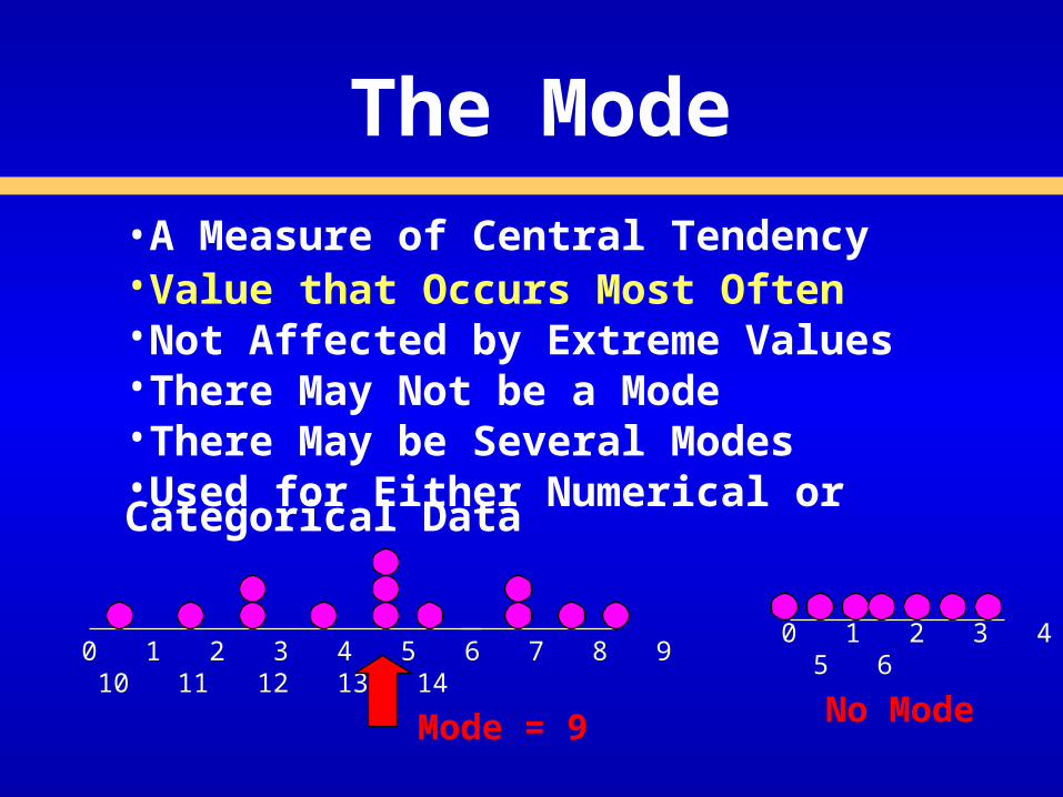
The Mode

0 1 2 3 4 5 6 7 8 9 10 11 12 13 14

Mode = 9

•A Measure of Central Tendency•Value that Occurs Most Often•Not Affected by Extreme Values•There May Not be a Mode•There May be Several Modes•Used for Either Numerical or Categorical Data

0 1 2 3 4 5 6

No Mode

Midrange

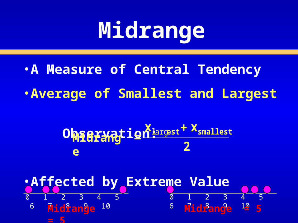
•A Measure of Central Tendency

•Average of Smallest and Largest

Observation:

•Affected by Extreme Value

2

xx smallestestl arg

Midrange

0 1 2 3 4 5 6 7 8 9 10

0 1 2 3 4 5 6 7 8 9 10

Midrange = 5 Midrange = 5

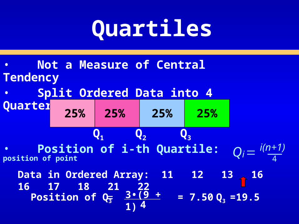
Quartiles

• Not a Measure of Central Tendency• Split Ordered Data into 4 Quarters

• Position of i-th Quartile: position of point

25% 25% 25% 25%

Q1 Q2 Q3

Q i(n+1)i 4

Data in Ordered Array: 11 12 13 16 16 17 18 21 22

Position of Q1 = 2.50 Q1 =12.5= 1•(9 + 1)4

Quartiles

• Not a Measure of Central Tendency• Split Ordered Data into 4 Quarters

• Position of i-th Quartile: position of point

25% 25% 25% 25%

Q1 Q2 Q3

Q i(n+1)i 4

Data in Ordered Array: 11 12 13 16 16 17 18 21 22

Position of Q3 = 7.50 Q3 =19.5= 3•(9 + 1)4

Summary Measures

Central Tendency

MeanMedian

Mode

Midrange

Quartile

n

xn

ii

1

Summary Measures

Variation

Variance

Standard Deviation


Range

1n

xxs

2i2

Measures of Dispersion (Variation)

Variation

Variance Standard Deviation Coefficient of Variation

PopulationVariance

Sample

Variance

PopulationStandardDeviationSample

Standard

Deviation

Range

100%

X

SCV

Understanding Variation

• The more Spread out or dispersed data

the larger the measures of variation

• The more concentrated or homogenous the data the smaller the measures of variation

• If all observations are equal

measures of variation = Zero

• All measures of variation are Nonnegative

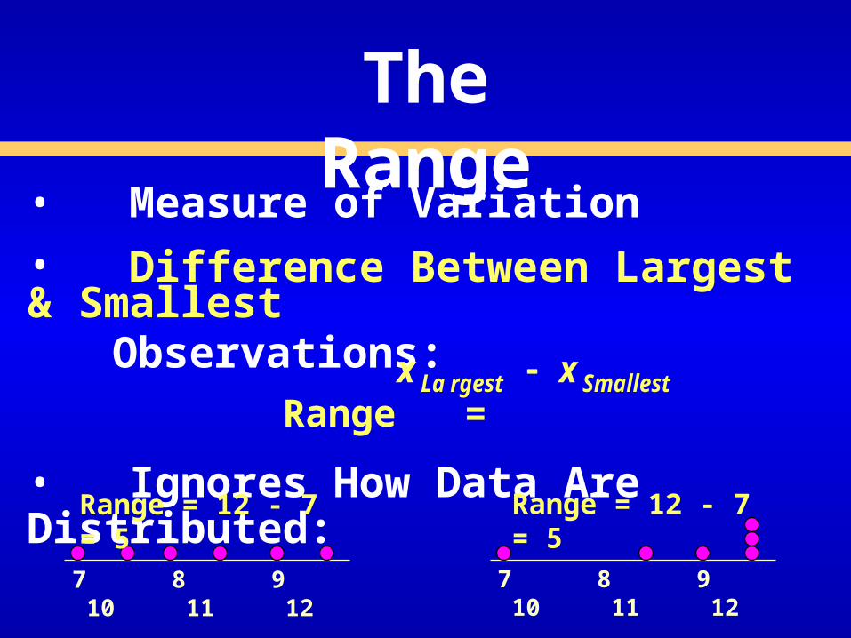
• Measure of Variation

• Difference Between Largest & Smallest Observations:

Range =

• Ignores How Data Are Distributed:

The Range

SmallestrgestLa xx

7 8 9 10 11 12

Range = 12 - 7 = 5

7 8 9 10 11 12

Range = 12 - 7 = 5

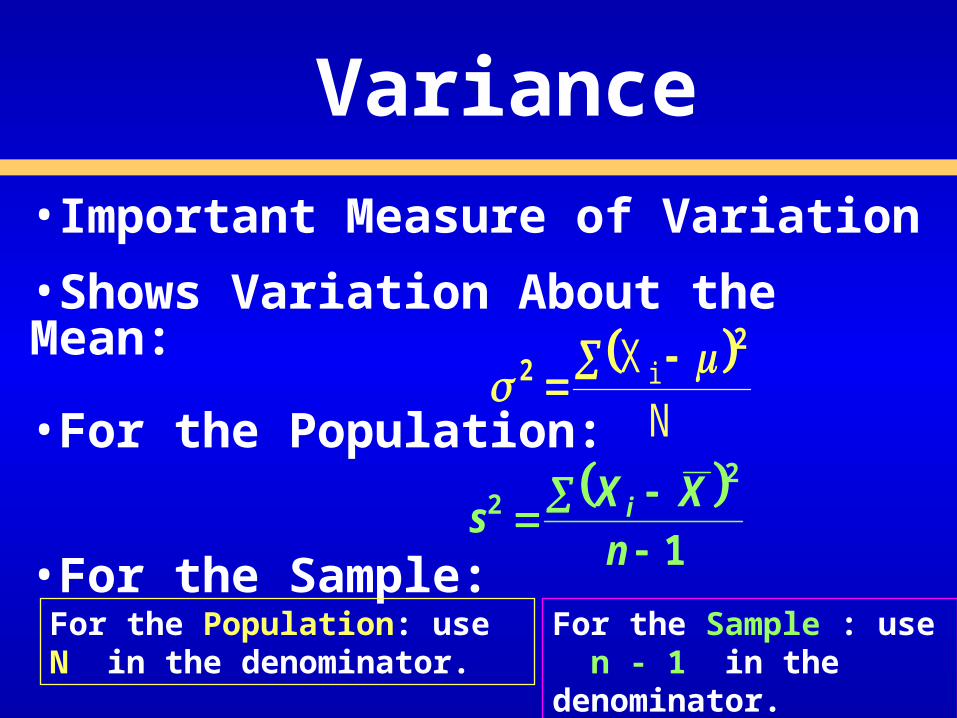
•Important Measure of Variation

•Shows Variation About the Mean:

•For the Population:

•For the Sample:

Variance

N

X i

22

1

22

n

XXs i

For the Population: use N in the denominator.

For the Sample : use n - 1 in the denominator.

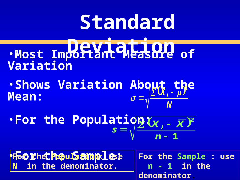
•Most Important Measure of Variation

•Shows Variation About the Mean:

•For the Population:

•For the Sample:

Standard Deviation

N

X i

2

1

2

n

XXs i

For the Population: use N in the denominator.

For the Sample : use n - 1 in the denominator.

Sample Standard Deviation

1

2

n

XX i For the Sample : use n - 1 in the denominator.

Data: 10 12 14 15 17 18 18 24

s =

n = 8 Mean =16

18

1624161816171615161416121610 2222222

)()()()()()()(

= 4.2426

s

:X i

Comparing Standard Deviations

1

2

n

XX is =

= 4.2426

N

X i

2 = 3.9686

Value for the Standard Deviation is larger for data considered as a Sample.

Data : 10 12 14 15 17 18 18 24:X i

N= 8 Mean =16

Comparing Standard Deviations

Mean = 15.5 s = 3.338 11 12 13 14 15 16 17 18 19 20 21

11 12 13 14 15 16 17 18 19 20 21

Data B

Data A

Mean = 15.5 s = .9258

11 12 13 14 15 16 17 18 19 20 21

Mean = 15.5 s = 4.57

Data C


•Measure of Relative Variation

•Always a %

•Shows Variation Relative to Mean

•Used to Compare 2 or More Groups

•Formula ( for Sample):

100%

X

SCV

Comparing Coefficient of Variation

Stock A: Average Price last year = $50

Standard Deviation = $5

Stock B: Average Price last year = $100

Standard Deviation = $5

100%

X

SCV

Coefficient of Variation:

Stock A: CV = 10%

Stock B: CV = 5%

Shape

• Describes How Data Are Distributed

• Measures of Shape: Symmetric or skewed

Shape



SymmetricMean = Median = Mode

-0.5 <0 < 0.5

Shape



Left-Skewed SymmetricMean = Median = ModeMean Median Mode

< -1 -0.5 <0 < 0.5

Shape



Right-SkewedLeft-Skewed SymmetricMean = Median = ModeMean Median Mode Median MeanMode

< -1 > 1 -0.5 <0 < 0.5

Box-and-Whisker Plot

Graphical Display of Data Using5-Number Summary

Median

4 6 8 10 12

Q3Q1 XlargestXsmallest

Distribution Shape & Box-and-Whisker Plots

Right-SkewedLeft-Skewed Symmetric

Q1 Median Q3Q1 Median Q3 Q1

Median Q3

A measure of the strength of linear

relationship between two variables X and

Y , and is measured by the (population)

correlation coefficient:

The numerator is the covariance

Correlation

cov ,xy

x y

X Y

The average of the products of the deviations of

each observation from its respective mean:

Covariance

1cov ,

N

i x i yiX Y

N

yx

Sample Correlation Coefficient

1

1

n

i ii

x y

rn

x yyx

s s

Correlation Coefficient ranges from –1 to +1

+1 perfect positive correlation

0 no linear correlation

-1 perfect negative correlation

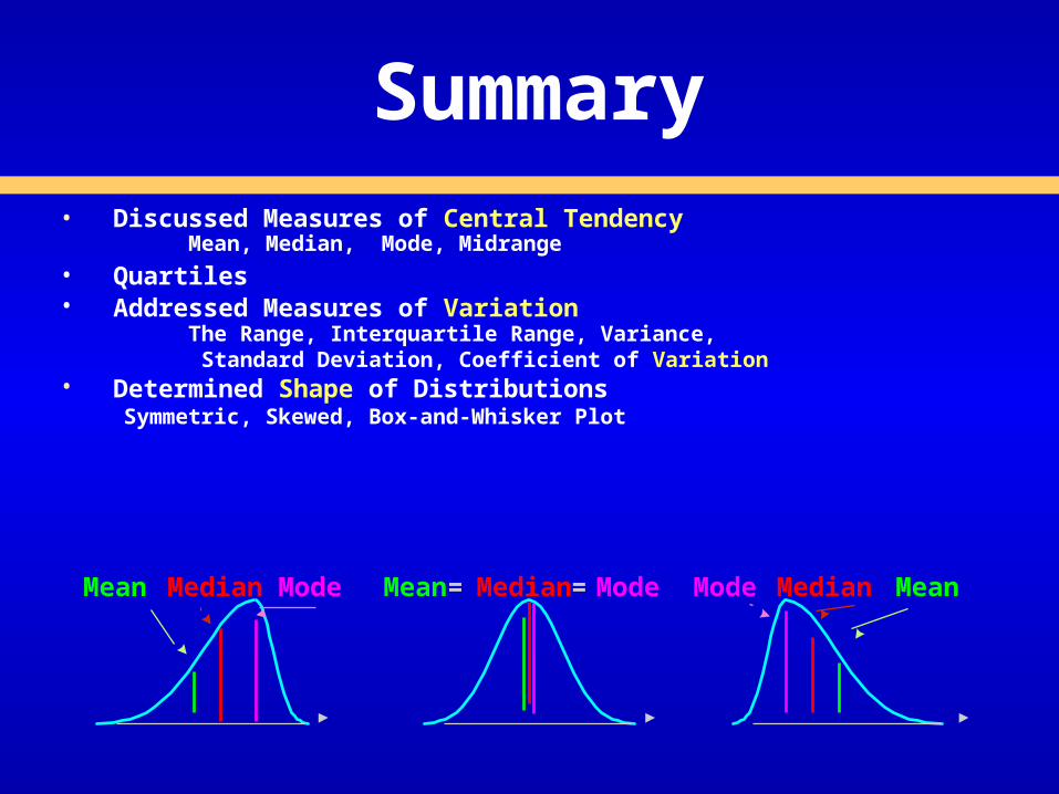
Summary• Discussed Measures of Central Tendency Mean, Median, Mode, Midrange

• Quartiles• Addressed Measures of Variation The Range, Interquartile Range, Variance, Standard Deviation, Coefficient of Variation• Determined Shape of Distributions

Symmetric, Skewed, Box-and-Whisker Plot

Mean = Median = ModeMean Median Mode Mode Median Mean

descriptive statistics a.a. elimam college of business san francisco state university

Documents