design and experimental validation of a carbon fibre
TRANSCRIPT

DESIGN AND EXPERIMENTAL VALIDATION OF A
CARBON FIBRE SWINGARM TEST RIG
Reno Kocheappen Chacko
A research report submitted to the Faculty of Engineering and the Built Environment, of the
University of the Witwatersrand, in partial fulfilment of the requirements for the degree of
Master of Science in Engineering
March 2013

i
Declaration
I declare that this research report is my own unaided work. It is being submitted to the Degree
of Master of Science to the University of the Witwatersrand, Johannesburg. It has not been
submitted before for any degree or examination to any other University.
……………………………………………………………………………
(Signature of Candidate)
……….. day of …………….., ……………

ii
Abstract
The swingarm of a motorcycle is an important component of its suspension. In order to test
the durability of swingarms, a dedicated test rig was designed and realized. The test rig was
designed to load the swingarm in the same way the swingarm is loaded on the test track. The
research report structure is as follows: relevant literature related to automotive component
testing, current swingarm test rig models and composite swingarms were outlined. The Leyni
bench, a rig specifically developed by Ducati to test swingarm reliability was shown to be
effective but lacked the ability to apply variable loads. The objective of this research was to
design and experimentally validate a swingarm test rig to evaluate swingarm performance at
different loads. The methodology, the components of the test rig and the instrumentation
required to achieve the objectives of the research were presented. The elastic modulus of the
carbon fibre swingarm material was calculated using classical laminate theory. The strains
and stresses within a swingarm during testing were analysed. The test rig was shown to be
versatile, accurate and efficient, with potential for future application. This research has shown
the benefit of test rigs for testing motorcycle components.

iii
To Ryan Chacko Preno

iv
Acknowledgment
First of all, to the almighty God, who strengthened me day in and day out. I take this
opportunity to thank Dr Frank Kienhofer, lecturer and researcher, within the school of
Mechanical, Industrial and Aeronautical Engineering, The University of the Witwatersrand
for providing me with all the support and guidance to carry out my project successfully and
for making my contribution to BlackStone Tek (BST) possible.
I express my sincere gratitude to my internal guides in BST, Mr Craig Goodrum and Mr
Damien Hawken who provided me with moral support and stood by me throughout the entire
duration of my project.
I express my profound sense of gratitude to the lecturers and the lab assistants of the
University of the Witwatersrand and Mr Hendrick and Mr Lawrence of BST. I am grateful to
the staff and management of the University of the Witwatersrand and BST for providing the
necessary facilities and encouragement for conducting the project.

v
Table of Contents
Declaration .................................................................................................................................. i
Abstract ...................................................................................................................................... ii
Acknowledgment ...................................................................................................................... iv
Table of Contents ....................................................................................................................... v
List of Figures ........................................................................................................................ viii
List of Tables ............................................................................................................................. x
List of Symbols ......................................................................................................................... xi
Nomenclature .......................................................................................................................... xiv
Chapter 1: Introduction .............................................................................................................. 1
1.1 Background ...................................................................................................................... 1
1.2 The Swingarm and Its Evolution ..................................................................................... 1
1.3 Ducati 1098 Single-Sided Swingarm ............................................................................... 3
1.4 Composites and its Development..................................................................................... 4
1.5 Chapter Summary ............................................................................................................ 5
Chapter 2: Literature Review ..................................................................................................... 6
2.1 Automotive Components Development in South Africa ................................................. 6
2.2 Development of Rigs for Testing ..................................................................................... 6
2.2.1 Automotive Component Test Rigs............................................................................ 7
2.3 Research Projects on Swingarm....................................................................................... 9
2.3.1 Swingarm Test Rigs .................................................................................................. 9
2.4 Swingarm Development Using Lighter and Stronger Materials.................................... 12
2.5 Motivation to Develop a New Swingarm Test Rig ........................................................ 13
2.6 Significance of Research................................................................................................ 13
2.7 Project Objectives .......................................................................................................... 14
2.7.1 Phase 1- Design of Test Rig.................................................................................... 14
2.7.2 Phase 2- Evaluation of Rig Performance ................................................................ 14
2.7.3 Phase 3- Evaluation of Results ............................................................................... 14
2.8 Organization of the Dissertation .................................................................................... 15
2.9 Chapter Summary .......................................................................................................... 15
Chapter 3: Methodology .......................................................................................................... 17
3.1 Product Requirement Specification (PRS)..................................................................... 17

vi
3.1.1 Requirements .......................................................................................................... 17
3.1.2 Constraints .............................................................................................................. 20
3.1.3 Criteria .................................................................................................................... 22
3.2 Design Approach ........................................................................................................... 26
3.3 System and Facility Requirements ................................................................................. 26
3.3.1 Mechanical Components ......................................................................................... 26
3.3.2 Data Acquisition (DAQ) System ............................................................................ 27
3.3.3 Higher Reliability Procedures or Modifications ..................................................... 31
3.4 Limitations of the Test Rig ............................................................................................ 31
3.5 Methodology to Calculate the Effective Elastic Constants of the Carbon Fibre
Swingarm ............................................................................................................................. 32
3.5.1 Design Approach .................................................................................................... 34
3.5.2 Assumptions ............................................................................................................ 34
3.5.3 Young’s Modulus, Volume Fraction, the Thickness and the Poisson’s Ratio of
Lamina ............................................................................................................................. 34
3.5.4 New Stiffness Values for Toray 700G According to the Orientation of Ply in
Tension and Compression ................................................................................................ 37
3.5.5 Effective Elastic Constants of the Swingarm for the 12 Layers ............................. 38
3.6 Chapter Summary .......................................................................................................... 39
Chapter 4: Results and Discussion ........................................................................................... 41
4.1 Introduction .................................................................................................................... 41
4.2 Variation of Effective Elastic Constants with Fibre Orientation for the 12 Layers ....... 41
4.3 Effect of Thickness ........................................................................................................ 44
4.4 Effect of Volume Fraction ............................................................................................. 45
4.5 Evaluation of Test Rig ................................................................................................... 46
4.5.1 Static Test................................................................................................................ 47
4.5.2 Dynamic Test .......................................................................................................... 47
4.6 Static Test Results .......................................................................................................... 48
4.6.1 Load vs. Time ......................................................................................................... 51
4.6.2 Strains vs. Time ...................................................................................................... 52
4.6.3 Stresses vs. Time ..................................................................................................... 52
4.6.4 Stress vs. Strain ....................................................................................................... 53
4.7 Dynamic Test Results .................................................................................................... 54
4.7.1 Load vs. Time ......................................................................................................... 55
4.7.2 Transmission History .............................................................................................. 56
4.7.3 Strain in One Second .............................................................................................. 56
4.7.4 Stresses in One Second ........................................................................................... 57
4.7.5 Stresses vs. Number of Cycles ................................................................................ 59

vii
4.7.6 Stress vs. Strain ....................................................................................................... 60
4.8 Chapter Summary .......................................................................................................... 61
Chapter 5: Conclusions and Future Work ................................................................................ 63
5.1 Conclusions .................................................................................................................... 63
5.2 Recommendations for Further Work ............................................................................. 64
References ................................................................................................................................ 65
Appendix A .............................................................................................................................. 69
A.1 Cost of Machined Components ..................................................................................... 69
A.2 Load Design .................................................................................................................. 70
A.3 Spring Design ................................................................................................................ 71
A.4 Motor Design ................................................................................................................ 74
A.5 Eccentric Bolt Design ................................................................................................... 75
A.6 Eccentric Shaft Design .................................................................................................. 77
A.7 Thread for the Hexagonal Bolt Design ......................................................................... 79
A.8 Bearing Design .............................................................................................................. 81
A.8.1 Bearing Over the Eccentric Shaft Design .............................................................. 81
A.8.2 Bearing Reactions .................................................................................................. 82
A.8.3 Bearing-2 Design ................................................................................................... 83
Appendix B .............................................................................................................................. 85
B.1 Strain Gauge Calibration ............................................................................................... 85
B.2 Load Cell Calibration .................................................................................................... 86
B.3 Equations for Strain Gauge Measurements ................................................................... 88
Appendix C .............................................................................................................................. 89
C.1 Young’s Modulus, Volume Fraction, the Thickness and the Poisson’s Ratio of Lamina
.............................................................................................................................................. 89
C.2 New Stiffness Values According to the Orientation of Ply in Tension and Compression
.............................................................................................................................................. 90
C.2.1 Equations Used ....................................................................................................... 90
C.2.2 Variation of Elastic Constants with Fibre Orientation ........................................... 90
C.3 Effective Elastic Constants of the Swingarm for the 12 Layers ................................... 93
Appendix D .............................................................................................................................. 94
D.1 Effect of Thickness ....................................................................................................... 94
D.2 Effect of Volume Fraction ............................................................................................ 95
D.3 Variation of Dynamic Load .......................................................................................... 96
D.4 Classical Laminate Theory............................................................................................ 97
Appendix E ............................................................................................................................ 100
E.1 The English code ......................................................................................................... 100

viii
List of Figures
Figure 1.1 Ducati 1098 single-sided swingarm ......................................................................... 3
Figure 2.1 A rolling bench test rig (42) ................................................................................... 10
Figure 3.1 Six degrees of freedom of the swingarm in a real-life test ..................................... 20
Figure 3.2 The six degrees of freedom of the swingarm during the test ................................. 21
Figure 3.3 CAD model of the swingarm test rig for dynamic testing ...................................... 23
Figure 3.4 The swingarm static test rig .................................................................................... 24
Figure 3.5 Layout for data acquisition ..................................................................................... 28
Figure 3.6 Attachment of strain gauges on the swingarm-1 .................................................... 29
Figure 3.7 Attachment of strain gauges on the swingarm-2 .................................................... 29
Figure 3.8 Graphical user interface panel ................................................................................ 31
Figure 3.9 The swingarm layup, which has +45o/-45
o and 0
o/90
o orientations ....................... 33
Figure 3.10 Principle material axes in a unidirectional lamina (53) ........................................ 35
Figure 4.1 Variations of effective Young’s modulus and Poisson’s ratio with orientation ..... 42
Figure 4.2 Variations of effective shear modulus with orientation ......................................... 43
Figure 4.3 Variations of effective elastic constants for compression with orientation ............ 44
Figure 4.4 Variations of effective Young’s modulus with volume fraction ............................ 45
Figure 4.5 Variations of effective transverse and shear modulus with volume fraction ......... 46
Figure 4.6 Mechanical spring arrangement inside spring housing .......................................... 47
Figure 4.7 Variation of dynamic load to the eccentric radius .................................................. 48
Figure 4.8 Resultant forces and moments acting on the laminate ........................................... 49
Figure 4.9 Load applied during the static test .......................................................................... 51
Figure 4.10 Strains experienced during the static test ............................................................. 52
Figure 4.11 Stresses experienced during the static test ............................................................ 53
Figure 4.12 Stress-strain graphs for static testing .................................................................... 53
Figure 4.13 Effective load applied in one second .................................................................... 55
Figure 4.14 Strain readings from the dynamic test .................................................................. 56
Figure 4.15 Effective strains in one second ............................................................................. 57
Figure 4.16 Stresses experienced in each second during the dynamic test .............................. 58
Figure 4.17 Stresses experienced during the dynamic test ...................................................... 59
Figure 4.18 Stress-strain graphs for dynamic testing............................................................... 60

ix
Figure A.1 Dimensions of a spring .......................................................................................... 71
Figure A.2 Eccentric mechanism components and the electric motor ..................................... 74
Figure A.3 Eccentric system of the test rig .............................................................................. 75
Figure A.4 Eccentric shaft and its components ....................................................................... 77
Figure A.5 Hexagonal bolt and its components ....................................................................... 80
Figure A.6 Dimensions of a double row angular contact ball bearing .................................... 81
Figure A.7 Bearing reactions ................................................................................................... 82
Figure A.8 Dimensions of a deep groove ball bearing ............................................................ 83
Figure B.1 Load vs voltage graph ............................................................................................ 87
Figure C.1 Variations of Young’s modulus for Toray 700G with orientation ........................ 91
Figure C.2 Variations of shear modulus for Toray 700G with orientation .............................. 91
Figure C.3 Variations of Poisson’s ratio for Toray 700G with orientation ............................. 92
Figure C.4 Variations of elastic constants for Toray 700G with orientation ........................... 92
Figure D.1 Variations of effective elastic constants with thickness of composite .................. 95
Figure D.2 Laminate geometry and ply numbering system ..................................................... 97

x
List of Tables
Table 3.1 Capital cost analysis of electrical test rig ................................................................. 25
Table 3.2 Capital cost analysis of hydraulic test rig ................................................................ 25
Table 3.3 Technical data sheet ................................................................................................. 36
Table 3.4 Stiffness values of each laminate ............................................................................. 37
Table 3.5 Elastic constant values with orientation of ply for Toray 700G .............................. 38
Table 3.6 Effective elastic constants of the swingarm for the 12 layers .................................. 39
Table A.1 The cost of machined components within the factory ............................................ 69
Table A.2 Cost of components purchased ............................................................................... 70
Table B.1 Strain gauge calibration chart .................................................................................. 85
Table B.2 Load cell calibration data ........................................................................................ 86
Table D.1 Effect of thickness on elastic constants .................................................................. 94
Table D.2 Effect of volume fraction on elastic constants ........................................................ 96
Table D.3 Variation of dynamic load to the eccentric radius .................................................. 97
Table D.4 Calculated values for laminate thickness ................................................................ 98

xi
List of Symbols
A Area under which the stress acts
AC Alternating current
C Specific capacity
C0 Basic static load rating
D Diameter of shaft/bolt
D Outer diameter
d Inner diameter
Dd Coil diameter
Dh Diameter of guide sleeve
Dm Mean coil diameter
E Young’s modulus,
Ef Elastic modulus of fibre
Em Elastic modulus of matrix
E11 Longitudinal modulus of elasticity
E22 Transverse modulus of elasticity
F Torsional frequency
F Maximum load
Fa Axial force
Fa Alternating force
Fm Constant mean load for a period of fluctuating load
Fc Cyclic load
fn Natural frequency of the spring
Fmax Maximum force
Fmin Minimum force
Fp Total preload
Fr Radial force
Frc Rear wheel cyclic load
Frp Rear wheel total preload
g Acceleration due to gravity
G12 Longitudinal in-plane shear modulus
GF Gauge factor of strain gauge

xii
hp Horse power
Hz Hertz
K Spring rate
Kt Stress-concentration-factor for bending
Kts Stress-concentration-factor for torsion
kW Kilowatt
Lh Life in working hours
L0 Free length of spring
Ln Life in millions of revolutions
Ls Solid length of the spring
M Bending moment
N Speed of shaft
Na Number of active coils
nf Total number of spring coils
P Pitch of thread
Rf Rated frequency
RG Nominal resistance value of strain gauge
RL Lead resistance
RPM Rotations per minute
Se' Endurance limit
Se Cyclic stress
Sf Factor of safety
Ssa Fatigue strength in reversed shear
Ssm Ultimate shear strength
Sse Yield strength in shear
Sut Ultimate tensile strength
t Laminate thickness
Tc1 Thickness of composites
τa Alternating torsional stresses
τm Midrange torsional stresses
τmin Minimum torsional stresses
τmax Maximum torsional stresses
xy Shear stress in the x-y plane
Vc1 Volume fraction of composites

xiii
VEX Excitation voltage.
Vf Volume fraction of fibre
υf Poisson’s ratio of fibre
υm Poisson’s ratio of matrix
Vm Volume fraction of matrix
VO (strained) Measured output when strained
VO (unstrained) Measured output voltage when unstrained
υ12 Major Poisson’s ratio
υ21 Minor Poisson’s ratio
W Wahl correction factor
Wb Motorcycle weight
Wr Weight of rider and passenger
σ Stress
σx Longitudinal stress
σy Transverse stress
σm Midrange axial stresses
σa Alternating axial stresses
σmin Minimum axial stresses
σmax Maximum axial stresses
Strain
εs Calibration strain
εi Indicated strain
εx Longitudinal strain
εy Transverse strain
xy Average shear strain on the x faces along the y direction, and on the y face
along the x direction
xy Shear strain in the x-y plane
θ Angle to the reference axis
ρ Density
ρm Density of matrix
ρf Density of fibre

xiv
Nomenclature
BST BlackStone Tek
CAD Computer Aided Design
EDS Electro Dynamic Shaker
FEM Finite Element Model
LabVIEW Laboratory Virtual Instrumentation Engineering Workbench
LVM LabVIEW Measurement
MIDP Motor Industry Development Programme
NI National Instruments
NPD New Product Design and Development
OE Original Equipment
PRS Product Requirement Specification
R&D Research and Development
RBT Rolling Bench Test
TÜV Technischer Überwachungsverein

1
Chapter 1: Introduction
1.1 Background
Motorcycles are one of the most affordable forms of motorised transport in many parts of the
world. For most of the world's population, they are also the most common type of motor
vehicle. The swingarm is the main component of the rear suspension of a modern
motorcycle. It supports the rear axle while pivoting vertically to allow the suspension to
absorb bumps on the road.
Motorcycle manufacturers are continually striving to improve their products and make
components (e.g. the swingarm) lighter, stronger and cheaper. This research report details the
development of an innovative suspension rig to test the durability of a swingarm. The rig will
be used to develop improved swingarms.
This project has been completed with the industrial support of BlackStone Tek (BST). BST is
an aftermarket and original equipment (OE) supplier of carbon fibre motorcycle components
[1]. BST has recently developed a carbon fibre swingarm for the Ducati 1098 motorcycle
which will be tested on the suspension rig detailed in this report.
Before a new design is allowed into the market, it first has to undergo certain quality tests.
Since BST is approved by the German TÜV, quality tests have to be undertaken to ensure that
the swingarm adhere to all the necessary safety standards (Appendix E). One of these tests is
a fatigue test where a component has to run for 500 000 cycles at a given loading. After the
test, no fatigue cracks or failure of mechanical fastenings may be present [2].
1.2 The Swingarm and Its Evolution
Automobile suspension systems and swingarms play a vital role in influencing ride comfort
as well as handling dynamics [3]. The handling qualities of motorcycles are often of great
importance [4]. They affect the pleasure to be gained from the rider–machine interactions and
the safety of the rider. The right handling makes any move easy: it depends on several
elements such as gravity centre position, total weight, stiffness, steering geometry, wheel size
and driver-machine coupling [5].

2
Today’s state of the art suspension designs evolved over the years, through numerous
iterations [3] [6]. Investigations of the dynamics and the stability of motorcycle components
have been conducted to improve the handling of motorcycles [7] [8] [9]. Comfort is also
important to minimize the driver’s stress; and thus suspension performance is crucial [6] [10].
Excessive flexibility of motorcycle components causes a phase lag which is difficult for the
driver to control. Because of low stiffness values, the driver feels the motorcycle as being
very heavy [11]. Motorcycles with a higher stiffness will have a greater responsiveness and
handling.
The functions of a motorcycle frame (chassis and swingarm) are of two basic types: static and
dynamic. In the static sense the frame has to support the weight of the rider or riders, the
engine and transmission and the necessary accessories such as fuel and oil tanks [12]. For
precise steering the frame must resist twisting and bending sufficiently to keep wheels in their
proper relationship to one another regardless of the considerable dynamic loads imposed by
power transmission, bumps, cornering and braking.
The main components linked to the chassis are the swingarm on the rear and the fork, which
steers and damps, on the front. As a motorcycle travels down the road, bumps and road
surface irregularities send dynamic loads through the rear wheel, forcing it upward. These
dynamic loads push against the swingarm, which moves vertically against its pivot point. The
vertical motion is dampened and absorbed by the suspension system, which rebounds and
pushes the swingarm back towards the ground to prevent a loss of traction [5] [13].
An excessive strain either on the swingarm or of the chassis has a bad effect on the steering
manoeuvre producing a thrust which is felt by the rider [14]. A procedure to measure these
strains on a swingarm is a necessity to identify the forms of instability that can compromise
the safety of the rider. The swingarm links the suspension to the wheel so its elasticity can
significantly change the vehicle set-up. Adding another spring in series to the shock absorber
can produce an unpredictable behaviour of the vehicle, thus reducing rider confidence.
Therefore the swingarm must have the maximum possible stiffness without compromising its
weight. Nowadays the structural optimisation of the swingarm is strategic for motorcycle
performance improvement [13].

3
Over the last twenty years a non-stop evolution has led to stronger and stiffer swingarms due
to the increased engine power [8]. At the beginning, a swingarm was simply a fork with two
tubed arms and pick up points for the dampers, and a crossed cylinder as pivot location [3]
[6]. This kind of swingarm was very weak, as all arms could swing freely from each other
causing large deformation. Over the time the size of the arms (diameter and thickness)
progressively grew until Yamaha made a new trellis scheme swingarm which was much
stiffer.
Nowadays swingarms are mostly made with two boxed beams and many stiffening elements
and ribs, and it is more and more uncommon to see a trellis model. Racing motorcycle
swingarms have to be a lot stiffer because of the static and dynamic loads they take.
1.3 Ducati 1098 Single-Sided Swingarm
Unlike most traditional constructions, essentially symmetric (forks), the Ducati 1098
swingarm exhibits a single-sided configuration as show in Figure 1.1, in that it entirely
develops along the left side of the wheel. The advantages that the single-sided swingarm
enjoys over the fork solution are the suggestive appearance and the fast wheel access. The
time reduction for changing the tyre and for testing different ratios of the chain transmission
is particularly useful in competitions [13]. Also the torsional stiffness can be made insensitive
to tightening of the wheel spindle, thus eliminating the disturbing attribute of the classical
design [15].
Figure 1.1 Ducati 1098 single-sided swingarm

4
The disadvantage of the single side swingarm is the reduction of the lateral bending stiffness
at the same weight condition. This can significantly degrade the curve stability and the
handling. The swingarm structure consists essentially of five connection points (Figure 1.1).
The two spreads are provided with holes supporting the swingarm pivot which joins the
swingarm to the frame with a swingarm pivot. The rear suspension is connected to the middle
of the arm by means of a two pins: two slots house the end of the shock absorber and the
extremity of the tie rod. Lastly the hub connects the swingarm to the rear wheel.
The stresses in swingarms are mainly affected by the rear suspension load; the most
dangerous stress level occurs when the load of the strut and the shock absorber are maximum
[13]. This happens slightly before the maximum shortening of the shock absorber because of
the damper effect and the complex interaction between the tyre and the road, i.e. the load
condition becomes more critical when riding over bumps.
Composite materials offer significant weight reduction opportunities and minimise stress
concentration areas while making the product stiffer. A study done by Bruderick et al. [16]
shows that the 2003 Dodge Viper was the first automotive to have its body structure
redesigned in carbon fibre. Mass reductions and stiffness improvements in the body structure
were the key achievements.
This process and material gave the design team great flexibility in consolidating the parts and
increasing the function of the system. A carbon fibre swingarm was thus developed [17]. This
new product enables the geometric freedom to improve frame design, resulting in improved
vehicle performance.
1.4 Composites and its Development
For motorcycles, the chassis needs to be lighter to improve both fuel efficiency and operating
performance. Some components of super sport models are currently being made of
aluminium or magnesium alloys [18] [19]. Composites have about two-third of the specific
weight of aluminium alloys and the high specific strength, provides a better solution [15]
[17]. A high degree of rigidity is required for a motorcycle swingarm because torsional,
vertical and horizontal bending forces are applied to it during its life.

5
In modern terms the word “composite” is often referred to a matrix material which is
reinforced with fibres [20]. The compositions are combined on a microscopic scale through
physical rather than chemical means, where the matrix is more soft and ductile than the
reinforcing fibre. Metals are usually isotropic in nature i.e. their properties are not dependent
upon direction whereas composites are anisotropic or at best orthotropic. Thus they show
variation in their mechanical properties according to the direction of the orientation of fibre.
[21].
The manufacturing method used can have a marked impact on the composite, thus
manufacturing takes on increased significance. A carbon fibre is a long and thin filament
which is about 5-10 μm in diameter and has a crystal bonding of carbon atoms which are
more or less aligned parallel to the longitudinal axis of the fibre. This type of bonding makes
the fibre very strong.
1.5 Chapter Summary
The introduction presents background information on swingarms and their evolution. The
Ducati 1098 single-sided swingarm was described along with some fundamental concepts of
composite materials. This work aims to show the design and validation of a test rig to
perform quality tests on a carbon fibre swingarm.
A detailed literature review is given hereafter in Chapter 2 to establish what research has
been carried out in the following areas:
Automotive components development and development of rigs for testing.
Research projects on swingarm and swingarm test rigs.
Swingarm development using lighter and stronger materials.

6
Chapter 2: Literature Review
The literature review summarises research conducted on automotive test rigs and composite
swingarms and testing. The initiative to introduce a test rig to assess the durability of
swingarms is subsequently discussed along with the project objectives and the organization of
the dissertation.
2.1 Automotive Components Development in South Africa
South Africa has a history of automotive assembly since 1920. Today, the country is the
leading producer on the continent. There are approximately 250 first tier suppliers and in
excess of 300 second and third tier suppliers. Investment in vehicle assembly and component
manufacture has also increased at an annual rate of 12% [22].
The automotive industry is a volume driven industry and certain critical mass is a pre-
requisite for attracting the much needed investment in research and development (R&D) and
new product design and development (NPD). R&D investment is needed for innovations
which is the life-line for achieving and retaining the competitiveness in the industry [23].
Simulation and testing at component level form an important part of automotive product
development. The objective of any component level testing is to bring the road conditions to
the lab. A procedure to derive an input excitation profile capable of generating damage
similar to the road is required in any lab test.
2.2 Development of Rigs for Testing
In the highly competitive automotive world, automotive manufacturers are focussing their
efforts on shortening product development cycle without compromising performance and
reliability [4] [24]. This means reducing the testing time by identifying the failure modes
early in the development cycle and avoiding the overdesign of components by optimising
them to the required life [25] [26] [27]. Researches have also shown that a greater level of
stability can be achieved by properly optimizing the design parameters without
compromising the requirement of ride comfort [3] [4] [28].

7
It is very difficult to predict the future loading history of a motorcycle. One solution is to fit
strain gauges and other transducers on a motorcycle ridden on a variety of road-track
conditions. With sufficient testing, one can thus build up a picture of the load cycles of a
typical machine over its expected lifetime. The second solution is to build a test rig that can
simulate the road conditions [12]. The first is not an option since BST did not have any
motorcycles for testing purposes but they are willing to invest in a test rig.
Physical testing must be conducted to validate designs and to determine the accuracy of
simulation or virtual testing. Virtual testing cannot replace physical testing [29]. Physical
testing can be performed on test rigs to validate simulations if it reproduces the failures
realistically as it happens on the field [30]. A similar approach is required in this research to
develop a test rig that simulates exact road conditions to test the durability and performance
of swingarms.
2.2.1 Automotive Component Test Rigs
Durability test rigs have been built to test motorcycle components such as a rig to test the
effect of disk braking on the durability of front shock absorber tubes [31], the fatigue life of
centre stands [26], the fatigue life of motorcycle handlebars [28] [32], the fatigue analysis of
motorcycle front fenders [27] [33] and the fatigue life of exhaust systems [34]. Results are
generally obtained by measuring the strain on the component and then calculating the
corresponding stresses. Different parameters like strain and acceleration play a crucial role in
durability prediction, as they are required across the process from test track/lab testing, to
virtual testing, to fatigue life prediction [30].
Kharul et al. [27] [33] used an electro dynamic shaker (EDS) to test a motor cycle front
fender. Strain data were collected on the components while it was being tested on the test rig.
The results obtained from experimental and FE-based fatigue life prediction were compared
with the estimated target life. The component design was then optimised using the FEA
simulation. A durable design of the fender was developed within a short time eliminating the
design cycle time and product development cost.
Correlations between customer usage and laboratory testing of automotive components were
conducted by Kharul et al. [24] [30]. Three full vehicle evaluation test rigs that evaluate
various components in a vehicle were selected for establishing a correlation with road usage.

8
All three test rigs had different loading patterns and rig 1 in this analysis was a rolling test
bench. Two different approaches, namely, failure data based analysis and experimental data
based analysis were adopted to arrive at a final correlation between the structural test rigs and
the customer usage on the road. The results indicated a good comparison between the
approaches. The conclusion was drawn that a well-designed test rig can accurately predict the
failure of a component being tested and gives a real test track response.
Similarly Muthuveerappan et al. [35] showed that test rigs for determining the performance
of automobile parts with dynamic loading offer a versatile means of simulating the actual
working condition of parts. The data obtained from the data acquisition systems from test rigs
were more reliable in predicting the life of the parts and in establishing the safe working
regime for the materials used in manufacturing the parts as compared to pure simulation. In
conclusion, a well-designed test rig provides real test track response and makes the system
more versatile in accurately predicting the failure of the component being tested.
Crump et al. [36] demonstrated the use of a test rig to replicate a full-scale pressure loading
on a composite aircraft wing structure. Their work clearly demonstrated that test rigs can be
designed to accurately impart representative loads to obtain the mechanical performance from
composite structures using strain measurement techniques.
In a 2011 study, Ismail et al. [37] showed that the development of a test rig setup with
LabVIEW could achieve test automation which reduced product validation time and provided
accurate results to test for fault tolerance of a system. The testing although not precise was
considered to be more accurate than analytical model predictions [38].
Carroll and Carver [39] presented a process for defining the mechanical parameters of
laboratory test systems used in evaluating durability and performance properties of
motorcycle components. They stated that in order to evaluate various properties of
motorcycles, the process often leads to track testing, laboratory testing, or some combination
of the two [30]. Also, a successful test begins with a good mechanical design which involves
many complex factors to arrive at an optimal balance among cost, complexity, simulation
accuracy, and ease of use. By considering those design factors, the mechanical engineer is
more likely to arrive at a design that will recreate the desired test environment, measure

9
useful responses, and provide useful data for analysis and future work. All these factors were
considered in this research.
2.3 Research Projects on Swingarm
A survey of the literature showed that there has not been extensive research into the testing of
motorcycle swingarms using a test rig and even less into the development of composite
swingarms but there are some studied on using FEM on swingarms for optimisation process
[14] [40].
A study was done using FEM for radiation noise analysis of an electric scooter swingarm.
The study was able to reduce the radiation noise by 10 dB [41].
Armentani et al. [14] developed a finite element model (FEM) of a swingarm to test for its
torsional and lateral stiffness. Because of the gravity centre position, the weight distribution
they used was 60% on the rear wheel and 40% on the front wheel. Five experimental static
tests were carried out: three to test the lateral deflection and two to obtain the flexional and
torsional stiffness.
2.3.1 Swingarm Test Rigs
Motorcycles are subjected to a series of physical tests to ensure survivability when subjected
to static and cyclic loadings. The bump test is one of the critical life tests performed on a
motorcycle for evaluating the fatigue life of the frame [25]. Unlike automobiles, in laboratory
simulations of motorcycles, test rigs must hold the Motorcycle upright. During normal riding,
gyroscopic effects of the tyres and wheels hold the vehicle upright [4].
A specially designed test bench was made to test three motorcycle swingarms by Risitano et
al. [11]. It was designed especially for determining the torsional stiffness of the components,
the symmetries and similarities in behaviour between clockwise and counter clockwise stress.
The rig consisted of a rigid steel platform on which the swingarm was constrained.
Potentiometers and dynamometers were used to measure the movements and the loads
applied by a hydraulic jack. The rear suspension was replaced with non-deformable rigid strut
fixed to the test bench. The pin-wheel and the wheel hub were mounted on the swingarm for
all tests. The torque was applied at points where there are holes in the chain tensioner. The
experimental results were validated with FEM analysis and the average percentage error was

10
less than 4%. This rig was limited to torsional stiffness test on swingarms that are
symmetrical.
2.3.1.1 Comfort Bench Test or Rolling Bench Test (RBT)
Rolling bench test (RBT) is a common test widely spread throughout motorcycle/scooter
companies whose rules have not been standardized yet; thus being different from one
company to another. The RBT is a severe test designed for reliability study of some
motorcycle parts: indeed, by the RBT it is possible to apply high stresses on the vehicle
performing accelerated fatigue cycles. This test replaces the on road tests, with ensuing time
and cost-saving. During the RBT the vehicle frame complete with front and rear suspension
is placed above rolling drums as shown in Figure 2.1. A variable number of shaped obstacles
are arranged on the external surface of one of the two rollers.
Figure 2.1 A rolling bench test rig [42]
The RBT was simulated by means of commercial multi-body software by Ardiri et al. [42].
The aim of their paper was to obtain the spectral stresses acting upon the swingarm of a
scooter during the RBT, so as to evaluate its fatigue strength. The correlation between
experimental data and computed results were good with a discrepancy of less than 5%. Their
work demonstrated the accuracy and reliability of numerical simulation to drastically reduce
the time of real experiments and tests.
Kumar [5] presented an FEM analysis of a motorcycle swingarm in different loading
conditions for optimisation. The results were validated through experimental analysis using
an RBT.

11
Carfagni et al. [10] built a numerical model that reproduced the test of a scooter on a RBT.
The model simulated the dynamic behaviour of the chassis and the rear suspension of the
motorcycle. A shortcoming with the RBT [25] is that the static weight applied doesn’t count
the weight of the rider and passenger. Thus a modified roller bench called the Leyni test
bench that includes the static weight was designed by Ducati.
2.3.1.2 Leyni test bench
The Leyni test bench is used to conduct fatigue tests to verify the reliability of the main
bodies of a motorcycle. The rig incorporates a rolling rig for testing a motorcycle on which a
dummy is placed [12] [13] [18]. A compression beam is lowered on to the dummy pushing
down with a load of 1960 N (the weight of the pilot and his passenger).
Stefano and Simone [43] developed a structural optimisation method which Ducati used to
design an efficient swingarm structure, with a high stiffness to weight ratio, respecting the
constraints given by the stylists. The purpose was to maximize the swingarm torsional
stiffness while minimizing its mass. The study was carried out by simulating a Leyni test to
test the behaviour between the swingarm and the other components of the motorcycle
including the chassis and the suspension system.
By means of numerical simulations (using FEM analysis) and experimental tests (using the
Leyni test bench) the stress field of a Ducati Monster S4 R single-sided swingarm and the
dynamic behaviour of a Ducati chassis were tested by Cassani and Mancuso [13] and Piazza
[12] respectively. They both concluded that the numerical results agreed with the failures
seen at the Leyni bench tests after many hundred thousands of loading cycles.
Gaiani [18] redesigned the carbon steel swingarm to an aluminium swingarm for the Ducati
Monster S4 R. Different welding solutions were compared to optimise the design. He used
the Leyni bench to test the reliability of the new component by an accelerated fatigue test.
Finally he was able to apply automatic MIG-welding technique to assemble the parts of the
swingarm and thus increasing daily production from 28 units to 110 units. It was observed
during the Leyni test he conducted that, in a standard test, a maximum external loading of
5900 N on the motorcycle (excluding the weight of the motorcycle) occurs during the impact

12
of the step (Appendix E, test factor (Kr) of 1.431). This standard maximum load will be used
in this research.
The main advantages of the Leyni test bench are its flexibility, cheapness, the speed of testing
and repeatability. The drawbacks are the impossibility to apply horizontal forces and variable
loads. It is not possible to obtain fatigue stress curves at different load levels because the
applied forces are controlled by the motorcycle suspension dynamics and determined by the
interactions between the stepped drum, tyre, suspension frame, constraint and preload
systems [12].
2.4 Swingarm Development Using Lighter and Stronger Materials
Based on the stress analysis of a swingarm of a certain model, Iwasaki et al. [19] designed a
magnesium swingarm that had the same degree of deflection when subjected to a torsion load
as an aluminium swingarm. A prototype magnesium swingarm was designed and produced
by press forming and TIG-welding the rolled AZ31 and extruded AZ31 magnesium alloys
respectively, because they were easier to find on the market. They concluded that the
prototype magnesium swingarm was 10% lighter and had 60% more torsional rigidity and the
static strength of the prototype magnesium swingarm was similar or superior to that of the
conventional aluminium swingarm.
Modern swingarms are mostly made with two boxed beams and many stiffening elements
and ribs for it to be stronger and lighter. Racing motorcycle swingarms have increased
stiffness and strength because of the increased static and dynamic loads they bear. Composite
materials offer significant weight reduction opportunities and O’Dea showed that a 3.9 kg
aluminium swingarm could be redesigned to weigh 2.7 kg using carbon fibre [17].
A magnesium alloy Ducati 916 single-sided swingarm was redesigned with composite
materials for reduction in mass and mass moment of inertia at comparable stiffness by
Dragoni and Foresti [15]. The structural behaviour of the composite arm was optimised by
FEM in view of high stiffness and low weight. The final composite design exhibits an
increased torsional stiffness (+10%), together with reduced mass (-30%) and mass moment of
inertia (-40%). The mass reduction contributed to a brisker performance and to a more
responsive handling of the machine while the decrease in mass moment of inertia added to

13
the bumping, the rebounding characteristics of the rear suspension, improving road holding
on irregular tracks.
2.5 Motivation to Develop a New Swingarm Test Rig
A search of the relevant literature revealed that there are few published experiments
quantifying the performance and durability of a swingarm. A summary of existing models
and their shortcomings are as follows:
1. Ardiri et al. [42], Kumar [5] and Carfagni et al. [10] validated their results by
conducting experimental analysis using a RBT. But the static weight applied on an
RBT never counts the weight of the rider and pilot and limiting the accuracy of the
load applied to a real-life test.
2. Risitano et al. [11] model was limited to torsional stiffness test for symmetrical
swingarms.
3. Dragoni and Foresti [15] validated their single-sided Ducati 916 composite swingarm
with an FE model but were never compared to any experimental results for accuracy.
4. The simulated Leyni test bench by Stefano and Simone [43], Cassani and Mancuso
[13] and Piazza [12] validated their results by conducting experimental analysis using
the Leyni test bench which counts the weight of the rider and pilot. But the accuracy
of the model was limited due to the impossibility to apply horizontal forces and
variable loads.
Considering the above points, this study seeks to identify and validate a suitable accelerated
approach for durability and performance testing of motorcycle components, in particular
swingarms. The Leyni test bench developed by Ducati did not evaluate swingarm
performance at different loads, and therefore it is desirable to have a simplified test rig that
can quickly and easily predict swingarm performance and counter the drawbacks of the Leyni
test bench. A dedicated test rig has to been designed to replicate the loading that a swingarm
could experience on the test track. The rig will then be used to test the durability and
performance of swingarms.
2.6 Significance of Research
A normal procedure for any automotive component which undergoes any testing is as follows
[25] [26] [27] [38]: a test simulation is made using software like ADAMS or BikeSim.

14
Subsequently, the data obtained from this model are used in FEM software and the stresses
are predicted. The stress pattern helps in identifying the critical areas. The critical areas
identified are validated through experimental strain measurement. The validated model is
further used to optimise the design by reducing the stresses at critical areas to below the
acceptable limit. The final optimised frame will clear the test without any failure. This kind
of approach saves the need to conduct expensive iterative tests.
This project is part of a larger project to develop an optimised swingarm. The FEA and
optimisation were considered to be beyond the scope of this project, which is a 50/50 MSc. A
50/50 MSc is made up to 50% coursework and 50% research. The development and design of
a new swingarm test rig was considered sufficiently novel as discussed in section 2.5.
2.7 Project Objectives
To design and experimentally validate a swingarm test rig to be used for durability testing of
carbon fibre swingarms at varying loads.
2.7.1 Phase 1- Design of Test Rig
Design a test rig for the fatigue testing of a carbon fibre swingarm.
The test rig should:
Replicate the suspension of a Ducati 1098.
Apply the required loads for the static and the dynamic test.
2.7.2 Phase 2- Evaluation of Rig Performance
The system should be capable of:
Counting the number of cycles performed.
Capturing and storing the load and all strains experienced by the swingarm during
fatigue testing.
Controlling the speed of the motor.
2.7.3 Phase 3- Evaluation of Results
The Swingarm should undergo 1.2 million cyclic loads (Sf > two, more than twice
the BS code requirement) for BST management approval.
Determine the stresses within a swingarm during testing and show that the
swingarm will withstand a real-life test without failure.

15
2.8 Organization of the Dissertation
The article is organized as follows:
Chapter one provides an introduction to this research, the background, the research problem,
research question and the hypothesis. It provides the overall research setting.
Chapter two presents a review of relevant literature related to automotive component testing,
current swingarm test rig models and composite swingarms. The project objectives are
outlined in this chapter.
Chapter three provides details on the methodology used in this research for the design of the
rig and to calculate the modulus of the carbon fibre swingarm. The chapter contains details of
how the rig was designed to make it as realistic as a real-life test and the detailed design of
the major components of the rig.
Chapter four presents the results and discussion of this research, including detailed outcomes
and assumptions. This section also covers details of the variable loading system for the static
and dynamic test rig to overcome the drawbacks of the current swingarm test rig models.
Chapter five provides a conclusion of the results of this research and recommendations for
further research.
2.9 Chapter Summary
The review of the literature began with a look at the current state of automotive component
development. Research examples of successively developed automotive test rigs were
described. A number of research projects on swingarms and the swingarm test rigs were
reviewed. Lastly, studies on swingarm development using lighter and stronger materials and
the need to develop a new test rig to assess the durability of swingarms were discussed along
with the project objectives and the organization of the dissertation.
In the light of the published literature, the significance of this research lies in the following
areas:
1. A research gap exists to develop a test rig, which incorporates the benefits and
overcomes the shortcomings of the Leyni test bench, which can assess carbon fibre

16
swingarm performance at varying loads. The test rig is able to include the loading of
the motorcycle pilot and passenger as a variable load.
2. There are no published results of a carbon fibre swingarm test and as a result the
safety of using such is unknown. Published carbon fibre test results would further the
application of composites in South Africa.
From these discussions on automotive component testing and test rigs, it is clear that the
accuracy of parameters like strain, acceleration etc. play a crucial role in durability prediction
since exposure to vibration may result in injuries to the rider/occupant and affect the
reliability and performance of the whole motorcycle. These results measured using a data
acquisition system can be used for refining a finite element analysis for future design
improvements.

17
Chapter 3: Methodology
This section covers details of the methodology used in this research using a well-defined
product requirement specification (PRS) technique. The different concepts considered for the
design of the rig and the detailed final concepts were defined. Finally the methodology to
calculate the effective modulus of the carbon fibre swingarm is presented.
3.1 Product Requirement Specification (PRS)
The Product Requirement Specification (PRS) [39] [44] will discuss the test and all
functional requirements of the rig to be designed. Relevant aspects of performance,
manufacture, operability and cost are considered to decide on the final concept from the
various alternative designs. The mechanical concepts of the test rig are outlined and all
additional development of the final concept, showing the comparison of functions during a
real-life test and while using the test rig, with respect to the product being tested. Lastly, the
limitations of the test rig are discussed.
3.1.1 Requirements
3.1.1.1 Describing the Test
The specimen to be tested is a Ducati 1098 single-sided carbon fibre swingarm as shown in
Figure 1.1 whose five connection points were described in chapter 1. The connection points
have aluminium inserts to enable the carbon structure to be attached to the motorcycle
suspension, frame and wheel system.
The goal of this test is to replicate the suspension of a Ducati 1098 to find the durability of
the swingarm through a static and dynamic test; both by reproducing the same loads the arm
experiences during a real-life test. For motorcycles, which are typically considered fair-
weather vehicles, environmental considerations are often secondary concerns. For durability
purposes, taking in to account the environmental factors, a higher safety factor (Sf > two, i.e.
1.2 million cycles, more than twice the BS code requirement for BST management approval)
is considered in this research.

18
3.1.1.2 Loading design
The static load due to the rider and the passenger is 1960 N (assuming weight of 100 kg per
person). The static load due to the weight of the motorcycle is 2158 N. The total static load is
therefore 4118 N (Equation A.2). The weight distribution was estimated as 60% on the rear
wheel and 40% on the front wheel [14] therefore total static load on the rear wheel is 2471 N
(Equation A.4).
A maximum external loading of 5900 N on the motorcycle (excluding the weight of the
motorcycle) occurs during the impact of the step of the Leyni test bench [18] (Appendix E).
The cyclic loading was thus calculated as 3940 N (Equation A.1). Therefore the maximum
load on the rear wheel is 4835 N (Equation A.5). Therefore in experimental testing, the
minimum and maximum loads applied in the vertical direction are 2471 N and 4835 N
respectively.
Specifications of the Test Rig
For dynamic test rig
No of cycles = 1.2 million cycles per test
Maximum preload on swingarm = 2471 N
Maximum cyclic load on swingarm = 2364 N
Minimum load applied on swingarm = 2471 N
Maximum load applied on swingarm = 4835 N
Dynamic loading frequency = 210 RPM
For static test rig
Maximum load on swingarm = 7350 N
3.1.1.3 Functional Requirements
Defining the test process and the constraints early in the system development stage will
reduce the number of design iterations and avoid expensive and time consuming mechanical
changes after the system is built. Recreating the exact conditions of a real-life test in the
laboratory test by reproducing the same loads the arm experience, will generate a more
accurate test result. Consequently the laboratory test must replicate the degrees of freedom of
the real-life scenario.

19
Degrees of Freedom
The six degrees of freedom of the swingarm in a real-life test during its operation are
identified (Figure 3.1):
The arm swings along the vertical direction during bumps or road surface
irregularities, and the vertical motion is determined by amount of road force acting on
the swingarm through the rear wheel forcing the arm upwards.
The arm is rigidly connected to the frame through the two spreads of the swingarm
pivot and thus preventing all horizontal motion (in the direction the motorcycle
travels) of the arm.
The arm is rigidly connected to the frame and the suspension system through the two
spreads of the swingarm and the shock absorber respectively to prevent any lateral
motion to the arm.
The arm swings about the lateral axis (pitch motion) with respect to the swingarm
pivot due to the bearing in the two spreads of the swingarm during its motion over
bumps.
The arm is rigidly connected to the frame and the suspension system through the two
spreads of the swingarm and the shock absorber respectively to prevent any roll
motion (rotation about the longitudinal axis) and yaw motion (rotation about the
vertical axis) to the arm for all non-cornering motions of the motorcycle. But during
cornering the wheel undergoes roll and yaw motion creating a bending and twisting
moment on the arm.

20
Figure 3.1 Six degrees of freedom of the swingarm in a real-life test
3.1.2 Constraints
The test is intended to have only one specimen tested at a time to 1.2 million cycles. The test
rig at BST will be operated by a skilled engineer or a technician at all times. The machine
will be used in a testing research environment; the installation of the test piece can be done
by some manual assembly and installation time. The test is not a non-stop continuous
process, as in the real-life case, the system can have scheduled maintenance in between and is
capable of accepting any down time for unexpected failures of the test equipment. The test rig
will also be bolted to the existing base of a lathe.
The test rig has to be designed in such a way that BST can perform the test accurately. But
the more accurate the machines have to be, the more expensive it becomes. So the engineer is
faced with a dilemma and in the end has to find a balance between the accuracy and cost of
the testing machine.
3.1.2.1 Test Rig Functional Constraints
Defining the test rig functional limits and constraints can avoid expensive and time
consuming mechanical changes after the system is built. The degrees of freedom during the
rest are defined for better comparison with a real-life test.

21
The exact six degrees of freedom of the swingarm during the test are identified as controlled,
restrained, or free (Figure 3.2):
The vertical motion of the swingarm hub is restrained by a horizontal slider.
The horizontal/longitudinal motion (in the direction the motorcycle travels) is
restrained by angle plate 2 which is attached to the base plate. The angle plate is
connected to the arm through the swingarm pivot and the two plummer blocks.
The lateral motion is restrained by the angle plate 1 which is attached to the base
plate. The angle plate is connected to the arm through the two rods replicating the
suspension system and the rocker arm.
The pitch motion (rotation about the lateral axis) is restrained by the slider mechanism
as it swings about the swingarm pivot.
Yaw motion (rotation about the vertical axis) and roll motion (rotation about the
longitudinal axis) is restrained by the swingarm pivot, the two plummer blocks, the
two rods replicating the suspension system and the rocker arm, which are all attached
to the two base plates along with the slider mechanism.
Figure 3.2 The six degrees of freedom of the swingarm during the test
The condition of bending and twisting moment acting on the arm during cornering of the
motorcycle is not taken in to consideration during both the tests. Since the road bump load is
much higher than the bending or twisting moment acting on the arm, the moments were

22
neglected. Normally a specially designed test bench like the one by Risitano et al. [11], is
designed to apply moments. Hence a separate project as future work will be initiated to
modify the rig.
3.1.3 Criteria
3.1.3.1 Proposed Methods of Test Rigs
The rig should test the swingarm specimen for 1.2 million cycles and thus all designed rig
parts should be capable to withstand many times more (effectively infinite) cycles for the
dynamic test. The rig should also be capable of applying variable loads.
Concept 1: Electrical Swingarm Test Rig
For dynamic testing
The test rig will consist of the following main components:
3 phase 4 kW AC motor.
Electronic motor controller.
Plummer blocks.
An eccentric mechanism to convert rotational to translational movement (Figure A.2).
A spring mechanism and housing.
A slider mechanism.
Angle plates to hold the swingarm (Figure 3.2).
A CAD model of the basic layout of the swingarm electrical test rig for dynamic testing is shown in
Figure 3.3, revealing the orientation of the motor, plummer blocks, springs, swingarm etc. These
components are to be mounted on a base plate, which is to be bolted to the existing base of a lathe.

23
Figure 3.3 CAD model of the swingarm test rig for dynamic testing
Concept 2: Hydraulic Swingarm Test Rig
For dynamic testing
The hydraulic test rig will have many components similar to the electric test rig but will
replace the electric motor along with the eccentric mechanism with a hydraulic system. The
eccentric mechanism is not used because direct force from the hydraulic piston will be
applied to the spring housing.
The test rig will consist of the following main components:
Hydraulic power system.
Hydraulics electronic control box.
Hydraulic cylinder.
A spring mechanism and housing.
A slider mechanism.
Angle plates to hold the swingarm.
No CAD models were made since this concept was rejected by BST management as
explained in section 3.1.3.2.
For static testing
The static test rig for both concepts will be the same. Although the static test rig is similar to
the dynamic test rig, a hydraulic jack with a hydraulic ram attached to an angle plate for
proper alignment, along with a chain will replace the electric motor, the eccentric mechanism,
the springs and its housings as shown in Figure 3.3. Thus the range of static load applied on

24
the swingarm will depend of the hydraulic ram capacity. The swingarm and its connection to
the base plate through the angle plates are exactly as in the dynamic test rig. The hydraulic
jack was chosen to be part of the test rig because of its availability in the bearing assembly
department of BST enabling cost reduction to the test rig.
The test rig will consist of the following main components:
Hydraulic jack.
Hydraulic ram.
Chain.
Angle plates to hold the swingarm.
Figure 3.4 The swingarm static test rig
3.1.3.2 Decision Factor
The decision was evaluated relative to budget, available materials and equipment,
manufacturing techniques, schedule, etc. BST have access to steel/aluminium rods or blocks
of any size from nearby factory outlets and CNC machines available within the factory,
which enables all aluminium/steel components to be machined with low cost. Thus with
proper design, low cost components of the rig can be made within the factory. The capital
cost of machined components with-in the factory followed by the cost of components
purchased which are common for electric and hydraulic test rig are given in Appendix A.1.

25
Capital Cost Analysis of Concept 1: Electrical Test Rig
Table 3.1 Capital cost analysis of electrical test rig
Components and specifications QTY
Price
(Inc.
VAT)
Total (R)
(Inc.
VAT)
4 kW electric motor, 1400 RPM 1 1825 1825
Movitrac motor controller 1 2600 2600
2 plummer bearings for eccentric mechanism 2 324 648
Bearing for con-rod 1 220 220
Total cost of purchased components (R) 10343
Total cost of machined components (only for electrical test rig) 1125
Total cost of machined components (common for electrical and hydraulic) 1501
Total cost of Electrical test rig 18262
Capital Cost Analysis of Concept 2: Hydraulic Test Rig:
Table 3.2 Capital cost analysis of hydraulic test rig
Components and specifications QTY
Price
(Inc.
VAT)
Total
(R) (Inc.
VAT)
Hydraulic power system, 5 hp, featuring reservoir,
electric motor and pump 1 30000 30000
Hydraulics electronic control box 1 6000 6000
Hydraulic cylinder, double-acting, 4in. Bore, 8in.
Stroke 1 3500 3500
Hydraulic hose, 1/2in. * 30in.l, 3500 psi 2 300 600
Other hydraulic accessories 1500 1500
Total cost of purchased components (R) 10343
Total cost of machined components (common for electric and hydraulic) 1501
Total cost of Hydraulic test rig 53444
From the above capital cost analysis, the hydraulic test rig costs almost three times the cost of
the electrical test rig. Even though most fatigue testing machines use hydraulic actuators to
perform the test, the Technical Director of BST wanted their rig to consist mostly of off-the-

26
shelf products for cost reduction. Thus the electrical test rig was considered as the final
concept which consisted of a cylinder with two springs with an eccentric that has a
continuous adjustment to cater for varying load ranges.
As BST needed to pass the BS code for fatigue test as early as possible for mass production,
it was advisable from the BST management to move forward with the electrical test rig due to
a shortage of funds and also the delivery of the hydraulic system and its components could
take up to 3 months or more.
3.2 Design Approach
1. Determine the static and dynamic loads that a swingarm must withstand and that must
be reproduced by the test rig.
2. Design and fabricate the bearings and other components used for the test rig to
produce the above loading.
3. Assemble the test rig and attach all instruments for the evaluation of the rig
performance.
4. Preload the swingarm to the desired static load.
5. Start the dynamic machinery of the rig to apply the dynamic load.
6. Evaluate the performance of the rig to apply the static and dynamic loads
representative of the loading experienced on the test track.
3.3 System and Facility Requirements
The success of any overall test system is highly dependent on the correct integration of the
mechanical and electrical hardware, with the associated electronics, data acquisition,
software, and analysis [38].
3.3.1 Mechanical Components
The mechanical design of the swingarm test rig components are given in Appendix A. The
following components are the crucial components of the test rig and are the significant
contributors to the cost of the whole test system and is therefore worth the time to properly
evaluate it as it is done.
Spring Design (Appendix A.3)
Motor Design (Appendix A.4)
Eccentric Bolt Design (Appendix A.5)

27
Eccentric Shaft Design (Appendix A.6)
Thread for Hexagonal Bolt Design (Appendix A.7)
Bearing Design (Appendix A.8)
Take Heed
Since the dynamic test is a high velocity test, especially with high specimen mass, care must
be taken in the design to ensure that the specimen can be stopped if control of the test system
is lost. The acceleration requirement is important since the test runs on the basis that the total
load is applied throughout each test cycles. Thus a Movitrac electronic motor controller
which can control the acceleration and equipped with an emergency STOP button was used.
Vibrations from the test rig can be transmitted into building structures, disrupt nearby
instrumentation, and disturb people working in the area. Thus the test rig was bolted to the
existing base of a lathe which has good vibration isolation.
3.3.2 Data Acquisition (DAQ) System
The main components of the DAQ system used to evaluate the performance of the swingarm
are:
1. Strain gauges/ load cell.
2. Data acquisition hardware – (consisting of NI SCXI-1000 chassis, SCXI-1600 control
card, SCXI-1521B strain gauge card, SCXI-1317 module).
3. The computer.
4. LabVIEW software.

28
A basic layout is shown in Figure 3.5 revealing the orientation of the load cell/strain gauges
and DAQ system.
Figure 3.5 Layout for data acquisition
3.3.2.1 Strain Gauges and Load Cell
Strain is the amount of deformation of a body due to an applied force. Strain gauges produce
electrical signals that the DAQ system measures. Signal conditioning accessories amplify
low-level signals and then isolate and filter them for more accurate measurements [45]. A
bonded resistance strain gauge is capable of measuring the minute changes in resistance
corresponding to strain [46]. Calibration of the strain gauges was done using the National
Instruments LabVIEW software features and the results are given in Appendix B.1.
Position of Strain Gauges
Five strain gauges were mounted on the swingarm for testing purpose as shown in Figure 3.6
and Figure 3.7.
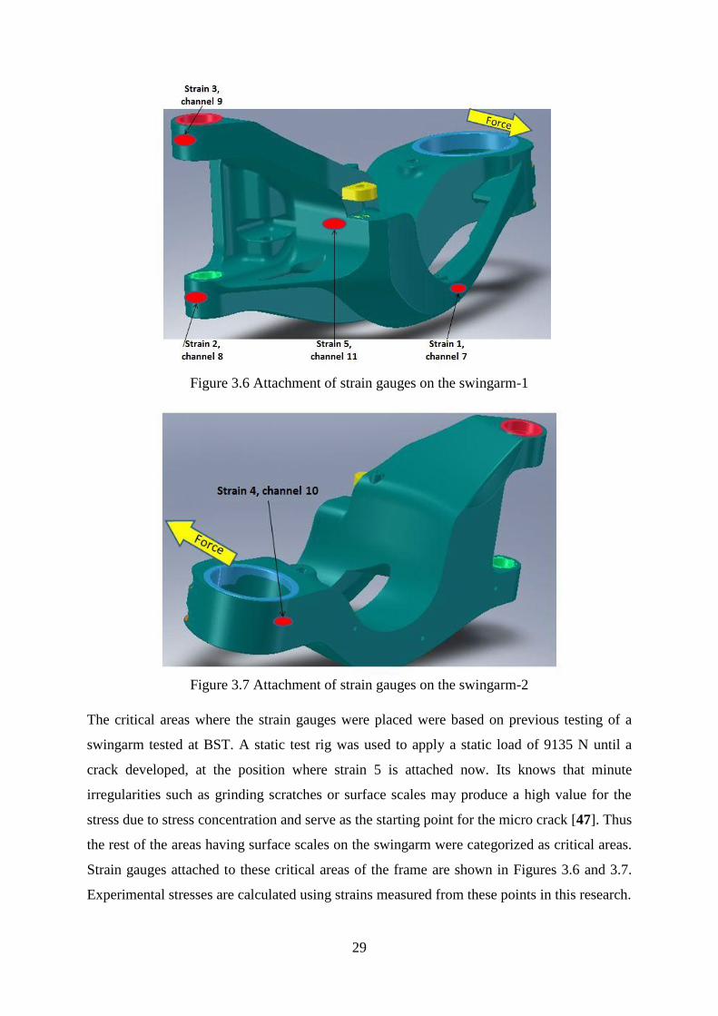
29
Figure 3.6 Attachment of strain gauges on the swingarm-1
Figure 3.7 Attachment of strain gauges on the swingarm-2
The critical areas where the strain gauges were placed were based on previous testing of a
swingarm tested at BST. A static test rig was used to apply a static load of 9135 N until a
crack developed, at the position where strain 5 is attached now. Its knows that minute
irregularities such as grinding scratches or surface scales may produce a high value for the
stress due to stress concentration and serve as the starting point for the micro crack [47]. Thus
the rest of the areas having surface scales on the swingarm were categorized as critical areas.
Strain gauges attached to these critical areas of the frame are shown in Figures 3.6 and 3.7.
Experimental stresses are calculated using strains measured from these points in this research.

30
The most commonly used load cell today is the strain gauge load cell. As their name implies,
strain gauge load cells use an array of strain gauges to measure the deformation of a structural
member and convert it into a voltage. A load cell with a maximum capacity of 5 ton was
placed as shown in Figure 3.3 to measure the load value applied to the arm. The load cell was
placed as close as possible to the test specimen for more accuracy.
The voltage signal was measured using the DAQ. Calibration of the load cell was done using
the NI LabVIEW software and the results are given in Appendix B.2. The equations used in
the strain gauge measurements are given in Appendix B.3
Take Heed
Lead wire resistance can cause a reduction in sensitivity because of the long wires used with
small gauge wires in it, which have greater resistance than the bridge completion wiring
within the measurement system. Strain gauge imperfections, lead wire resistance, and a pre-
strained installation condition will generate some nonzero initial voltage offset.
3.3.2.2 Software
LabVIEW is the platform and development environment for a visual programming language
from National Instruments. The graphical language is named "G". Execution is determined by
the structure of a graphical block diagram (the LV-source code) on which the programmer
connects different function-nodes by drawing wires. LabVIEW programs or subroutines are
called virtual instruments (VIs).
The graphical user interface panel used in this research for data acquisition using LabVIEW
is shown in Figure 3.8. When the stop button is clicked, the predetermined number of
samples is acquired and stored on the computer hard disk as a LabVIEW measurement file
(.LVM).

31
Figure 3.8 Graphical user interface panel
3.3.3 Higher Reliability Procedures or Modifications
The test was never a non-stop continuous process, and had scheduled maintenance in between
due to unexpected failures of the test rig components. And since the reliability of the whole
system depends on the reliability of each component in the system [48], modifications were
done to some components to increase the reliability of the whole system. Some of these
modifications or procedures to ensure higher reliability are listed below:
The single plummer block system (Figure3.3) was replaced with the two plummer
block system (Figure A.2). The new shaft rotating inside the two plummer blocks,
which extends from the eccentric hub was press forged by heating the eccentric hub to
180 0c
and cooling the shaft to -30
0c.
The two plummer block system lasted for over 1
million cycles compared to the 200 000 cycles of the single plummer block system.
A hydraulic press (available in BST bearing assembly department) was used to press
fit most components of the rig. All tolerances for the fit were designed according to
ISO standards.
3.4 Limitations of the Test Rig
It is difficult to simulate interaction between rider and vehicle. In a real-life test, the
vehicle response is substantially influenced by the posture, weight distribution and
characteristics of the rider and pillion. Also while moving over a bump, the rider is

32
separated from the vehicle (momentarily will be in air) and lands again onto the seat.
This phenomena causes tyre force variation [6].
The force of gravity acts on the vertical plane of the swingarm in a real-life test as
shown in Figure 3.1 but since the swingarm was placed laterally on the test rig (Figure
3.3, since it was the only option available to apply forces accordingly) the force of
gravity acting will be on the lateral side of the swingarm.
Neither of the two tests in this research included the dynamics of cornering, running
engine, wind, or temperature, since each additional condition adds considerable
complexity and cost to the test rig.
3.5 Methodology to Calculate the Effective Elastic Constants of the Carbon
Fibre Swingarm
A study on each layer was done to determine the stiffness of the layers (since data from
Toray was limited to Table 3.1) and combined to formulate the effective elastic constants of
the swingarm in tension and compression. Using the calculated values of the effective elastic
constants of the swingarm in classical laminate theory and Hooke’s law [49] [50], the stresses
in the swingarm can be calculated.
Unlike isotropic materials, carbon fibre composites are a man-made material that can be
made to satisfy virtually any mechanical property without changing the overall structural
shape of the part, they are entirely anisotropic. The ability to customize your fibre direction
allows you to only use as much material and fibre as you need; rather than waste material,
costs, strength, and weight in directions you don’t need. The high importance of laying down
patches of carbon fibre pre-preg in different orientations is due to carbon fibre having
maximum strength only along the lengths of the fibres.
Carbon fibre fabric comes in a variety of weaves that have different strength properties like
woven fabric or unidirectional fabric. The carbon fibre swingarm is made of 12 layers of two
different composites packed together at different orientations at BST, i.e. by placing 6 layers
of Toray 700S (unidirectional carbon) in 0o/90
o orientation and 6 layers of Toray 700G
(woven fabric) in +45o/-45
o orientation as shown in Figure 3.9. Toray carbon fibres are the
suppliers of carbon fibre sheets for the swingarm production in BST.

33
Figure 3.9 The swingarm layup, which has +45o/-45
o and 0
o/90
o orientations
Unidirectional carbon fibre is a reinforcement where all (or almost all) of the carbon fibres
are aligned in the same direction. The only thing holding the fibres together will be
occasional strands of either carbon or polyester running across the fibres at 90 degrees. A
unidirectional weave creates a carbon fibre sheet that’s very strong in the direction of the
fibres, but weak in the opposite direction. On the other hand, a woven fabric contains fibres
oriented on at least two axes, in order to provide great all-around strength and stiffness. A
sheet of woven fabric once cured can take flexural and tensile loads on multiple axes, and
even exhibits good stiffness properties off axis. A woven fabric was the norm for the
outermost covering of any carbon component for its traditional “weave” look appearance.
If a hole is punched in a unidirectional fabric it will compromise strength for the entire length
of the fibre, relying on the resin strength to distribute loading across the broken fibres. Unlike
on the weave fabric, strands punctured in one place, will behave at full strength within a very
short distance (typically one to two weave widths) from the damage [51]. But if a component
requires 70% strength in the horizontal direction and 30% strength in the transverse direction,
woven fibre would waste 40% additional material than unidirectional fibre to meet the same
requirements [52]. Thus the combination of the two would be ideal for better performance
and cost.
The swingarm is a complicated structure without symmetry but a high degree of rigidity and
stiffness is required all-around the structure because torsional, vertical and horizontal bending
forces are applied to it during its life (Figure 3.1). Thus a combination of a high strength,
standard modulus unidirectional fibre (Toray 700S) and enhanced adhesion properties and
tensile modulus woven fibre (Toray 700G) was used for the swingarm.

34
3.5.1 Design Approach
1. Determine the Young’s modulus, volume fraction, the thickness and the Poisson’s
ratio of each layer.
2. Calculate the new stiffness values according to orientation of ply in tension and
compression.
3. Determine the effective modulus and the Poisson’s ratio for the swingarm in tension
and compression.
4. Use the final effective elastic constant values in classical laminate theory along with
the measured strain values to determine the stresses in the swingarm.
3.5.2 Assumptions
While designing composite structures, the main problems faced are [49] [53] [54]:
1. Fibre waviness and variation in thickness are the most common type of defects in
composite material due to their complicated manufacturing process. This type of
material imperfection increases the strain in the localised region and can lead to
premature failure. Care should be taken in the manufacturing process to eliminate
fibre waviness and variation in thickness.
2. Non-uniform fibre strength is a characteristic of most current high-strength fibres.
Failure due to non-uniform fibre strength can be prevented by using a strong fibre-
matrix interface or a soft ductile matrix which permits the redistribution of the high
shear stresses.
Several assumptions were made when characterizing the lamina properties [50]:
1. The fibre and matrix material were assumed homogeneous.
2. The fibre and matrix material were assumed orthotropic.
3. The bonding between the fibre and matrix was assumed perfect, and thus strains
experienced by the fibre, matrix and the composite are the same in all directions.
3.5.3 Young’s Modulus, Volume Fraction, the Thickness and the Poisson’s Ratio of
Lamina
In the design of composite structures, it is often necessary to predict the strength of the
laminate. Since the laminate strength depends on the strength of the individual lamina from
which it is made. Most of the composite materials are made by stacking several distinct layers
of unidirectional or woven lamina. Each lamina or ply is made of the same constituent

35
materials, matrix and fibre. Figure 3.10 represents a unidirectional lamina with respective
longitudinal and transverse directions.
The stiffness of the lamina and laminate depends on three factors [53]:
1. Volume fraction of the constituent materials.
2. Thickness of each layer.
3. Orientation of the fibres with respect to a common reference axis [54].
Figure 3.10 Principle material axes in a unidirectional lamina [53]
X-Axis - an axis in the plane of the laminate, which is used as the 0 degree reference
for designating the angle of a lamina.
Y-Axis - the axis in the plane of the laminate which is perpendicular to the x-axis.
Z-Axis - the reference axis, normal to the plane of the laminate.
X-Y Plane - the reference plane, parallel to the plane of the laminate.
Given data
Different carbon composite structures are formed from different combinations of matrices
and fibres, thus there were limited technical data about the carbon fibre composite used in
this research. Table 3.3 provides all technical data’s collected from Toray which were used
for the calculations of the lamina strength [55] [56] [57].

36
Table 3.3 Technical data sheet
Material 1- Toray 700S (Unidirectional)
Material 2- Toray 700G (Woven)
Areal mass, m700S = 300 g/m2 Areal mass, m700G = 380 g/m
2
No of lamina, n1 = 6 No of lamina, n2 = 6
Fibre
Fibre
Elastic modulus, Ef = 230 GPa Elastic modulus, Ef = 240 GPa
Poisson’s ratio, vf = 0.20 Poisson’s ratio, vf = 0.20
Volume fraction, Vf = 0.60 Volume fraction, Vf = 0.49
Density, ρf = 1800 g/m3 Density, ρf = 1800 g/m
3
Matrix (Epoxy Resins)
Matrix (Epoxy Resins)
Elastic modulus, Em = 4.5 GPa Elastic modulus, Em = 4.7 GPa
Poisson’s ratio, υm = 0.33 Poisson’s ratio, υm = 0.30
Volume fraction, Vm = 0.40 Volume fraction, Vm = 0.51
Density, ρm = 1250 g/m3 Density, ρm = 1250 g/m
3
Carbon Fibre [57]
Carbon Fibre
Shear modulus, G12= 4.4 GPa Shear modulus, G12= 5.5 GPa
Results
The equations used to calculate the Young’s modulus, volume fraction, the thickness and the
Poisson’s ratio of lamina are given in Appendix C.1. The results are calculated by
substituting the values from the above table in to the equations in Appendix C.1 and are
shown in Table 3.4.

37
Table 3.4 Stiffness values of each laminate
Toray T700S Toray T700G
E1 140 GPa 120 GPa
E2 10 GPa 9 GPa
G12 4.4 GPa 5.5 GPa
υ12 0.25 0.25
Tc 2.440 mm 3.091 mm
Total Thickness 5.530 mm
Vc 0.441 O.559
The rule of mixture model was selected for the analysis in this research. It is observed that the
elastic constants of a laminate are a function of the volume fraction, which in turn is a
function of the thickness of the body [49]. The thickness is higher in T700G since more areal
mass is present in it. The transverse modulus is matrix dominated and tends to be very low in
comparison to the fibre dominated longitudinal modulus.
Since the composite structure is cured under vacuum in an autoclave at BST. No specimen
tests were conducted to compare the results with respect to the calculated material properties
because of the time and cost involved in the moulding and curing process for manufacturing
the test specimen required.
3.5.4 New Stiffness Values for Toray 700G According to the Orientation of Ply in
Tension and Compression
Composites are rarely used in the form of unidirectional laminates, since one of their greatest
merits is that the fibres can be arranged so as to give specific properties in any desired
direction. In order to calculate the properties of the woven fibre (T700G), which is orientated
at ± 45o direction to the unidirectional fibre (T700S), a method which can determine the
stress-strain relations for a lamina at an arbitrary orientation to the reference axes is required
[49] [50]. The equations used to calculate the new stiffness values according to the
orientation of ply in tension and compression for Toray 700G followed by the variation of
elastic constants with fibre orientation are given in Appendix C.2.

38
Results
The results are calculated by substituting the values from Table 3.3 in to the equations in
Appendix C.2 and are shown in Table 3.5.
Table 3.5 Elastic constant values with orientation of ply for Toray 700G
Old values New values
Tension Compression Tension Compression
E1 140 GPa 120 GPa E1 14.016 GPa 13.464 GPa
E2 10 GPa 9 GPa E2 14.016 GPa 13.464 GPa
υ12 0.25 0.25 υ12 0.274 0.224
G12 5.5 GPa 5.5 GPa G12 9.032 GPa 8.089 GPa
For tension and compression, fibre behaviour dominates the 0o/90
o behaviour, while matrix
behaviour dominates the +45o direction and at 45
o the value of E1 and E2 will be the same. It
is observed that the good properties in a particular direction come at the expense of poor
properties in another direction. These roles are reversed in the shear case, the +45o behaviour
is fibre dominated and thus this is the ideal angle at which the lamina will resist maximum
torsion. Hence a sensible approach to design a structure with all-around rigidity and stiffness
(like the swingarm), would be to ensure that the transverse and shear modulus are at its
maximum.
3.5.5 Effective Elastic Constants of the Swingarm for the 12 Layers
Since the swingarm has 12 layers of two different composites packed together at different
orientations, the resulting elastic constants will clearly be affected by the distributions of the
different species of fibre. Thus the results from the above two tables are combined to
formulate the effective elastic constants as a function of the volume fraction of the swingarm
in tension and compression. The equation used is given in Appendix C.3.
Results
The results are calculated by substituting the values from Table 3.4 and Table 3.5 in to the
equation in Appendix C.3 and are shown in Table 3.6.

39
Table 3.6 Effective elastic constants of the swingarm for the 12 layers
Tension Compression
E11 67.391 GPa 67.083 GPa
E22 12.244 GPa 11.936 GPa
υ12 0.264 0.235
G12 9.459 GPa 9.462 GPa
The combination of different lamina types and orientation results in a strength of 67 GPa in
longitudinal direction (50% less than initial lamina strength) and 12 GPa in shear direction
(more than 150% greater than the initial lamina strength) and thus creating a composite that
has high stiffness in all directions, to resist torsional, vertical and horizontal bending forces
acting on the arm, by taking advantage of the longitudinal strength of the unidirectional fibre.
3.6 Chapter Summary
The research methodology presents a structured approach in addressing the research problem
using a well-defined product requirement specification (PRS) technique. This discussed all
functional requirements of the rig to be designed. The different criteria were considered to
decide on the final concept from the various alternative designs. All design details of the
components in the test rig and instrumentation required to perform the desired objectives
were outlined along with the limitations of the test rig.
This rig is the first of its kind for swingarm testing and has highlighted a number of unique
aspects of the rig. There is significant scope for further work on this topic in performing error
analyses by comparing the FE model results with the test results and also in developing a
hydraulic test rig for improved reliability and accuracy. The final concept of the test rig offers
the following advantages:
1. The model is capable of overcoming the shortcomings of the previous test rig, the
Leyni test bench.
2. The model is capable of recreating all degrees of freedom and reproducing the same
loads the swingarm experiences in the laboratory test as in a real-life test. This system
is able to simulate road conditions in the laboratory for stress calculations.

40
3. Many complex factors were considered to arrive at an optimal balance among cost,
schedule, available materials and equipment, manufacturing techniques, complexity,
simulation accuracy, and ease of use.
4. With slight modification the model can test durability or even test torsional or
bending stiffness of different carbon fibre components at BST.
Since no data were available regarding the effective elastic constants of the carbon fibre
swingarm, a methodology to calculate this was developed. Using equations of composites,
the stiffness of each layer at 0o/90
o and 45
o was calculated and then combined to formulate
the effective elastic constants of the swingarm in tension and compression. These values are
used in the classical laminate theory to determine the stresses in the swingarm. The design
approach for each methodology was outlined, including the assumptions and limitations for
each test. The next Chapter deals with the results and discussion of the analysis on the
research data.

41
Chapter 4: Results and Discussion
4.1 Introduction
The discussion begins with a look at parameters that affect the final mechanical properties of
composites and some of the major parameters are discussed here with its effect on the current
design of the swingarm and thus validating how the swingarm test rig can guide the carbon
fibre swingarm to an improved design. Lastly, the strain gauged results of the static and
dynamic tests of the swingarm are discussed, validating that the swingarm can withstand a
real-life test without failure. Even though there are no published results available for the
carbon fibre swingarm in the literature of stresses and strains for comparison and error
analysis, the results of the static and dynamic test were compared to arrive at a good
correlation between the both.
4.2 Variation of Effective Elastic Constants with Fibre Orientation for the
12 Layers
A study is done to verify if the current model of the swingarm in which 6 layers of Toray
700S are 0o/90
o orientated and 6 layers of Toray 700G are +45
o/-45
o orientated, has
maximum strength and stiffness in the shear and transverse direction. The values for the
elastic constants of Toray 700S is taken from Table 3.4. These values are constants since
their orientation is fixed at 0o/90
o. The values for the elastic constants of Toray 700G is varied
according to fibre orientations from 0o to 90
0 using the equations from Appendix C.2. Then
the values for the effective elastic constants of the swingarm for the 12 Layers orientated at
angle from 0o to 90
o are calculated using the equation from Appendix C.3 and the results are
shown below.

42
4.2.1 For Tension
The effective longitudinal modulus, transverse modulus and Poisson’s ratio were varied with
fibre orientation angle from 0o to 90
o. The results are shown in Figure 4.1.
Figure 4.1 Variations of effective Young’s modulus and Poisson’s ratio with orientation
The effective longitudinal modulus is higher than the rest of the values in the initial stage as it
is the fibre property. The variation of Poisson’s ratio of the composite is less sensitive to the
fibre characteristics. The longitudinal modulus is at its maximum when the 700S and 700 G
are at 0o. The transverse modulus reaches its maximum when the 700G is at 90
o. The
effective shear modulus was varied with fibre orientation angle from 0o to 90
o and the results
are shown in Figure 4.2
0
20
40
60
80
100
120
140
160
0 15 30 45 60 75 90
E1,E
2 (
GP
a) &
υ(*
10
0)
Angle (deg)
E11
E22
v

43
Figure 4.2 Variations of effective shear modulus with orientation
The variation of shear modulus is less sensitive compared to others and thus it is shown in a
different graph for better visibility of the effect. The effective shear modulus starts to rise
from 0o and reaches its maximum when the 700G is at 45° to the fibre axis, the +45
o
behaviour is fibre dominated and thus this is the ideal angle at which the lamina will resist
maximum torsion, and falls to the initial value from +45o to 90
o. The shear stiffness of the
composite rises as the loading direction shifts away from the matrix axis, to the fibre axis at
45° and drops to the initial value as it shifts back to matrix axis at 90o. The shear stiffness of
the composite is less sensitive to the matrix characteristics as angle increases from 0o to 45
o,
being largely controlled by the fibre rigidity. Thus it will resist maximum shear at 45° angle,
which is achievable only in composites by changing the orientation which gives composites
its advantage over alloys and pure metals.
4.2.2 For Compression
The effective longitudinal modulus, transverse modulus, shear modulus and Poisson’s ratio
were varied with fibre orientation angle from 0o to 90
o under compression and are shown in
Figure 4.3.
0
1
2
3
4
5
6
7
8
9
10
0 15 30 45 60 75 90
G (
GP
a)
Angle (deg)
Gf

44
Figure 4.3 Variations of effective elastic constants for compression with orientation
Using fibre orientation, it is possible to create a composite that has high stiffness in all
directions by taking advantage of the longitudinal strength. The shear strength variation is
one of the principle advantages of composites. Thus the component will be designed to resist
all the forces acting in all directions. Since the swingarm must resist forces in all direction the
700S was orientated at 0o and the 700G was orientated at 45
o to give maximum strength and
stiffness in the shear and transverse direction along with a good longitudinal stiffness. The
values for the effective elastic constants of the swingarm for the 12 layers i.e. 6 layers of
Toray 700S in 0o/90
o orientation and 6 layers of Toray 700G in +45
o/-45
o orientation in
tension and compression are given in Table 3.6.
4.3 Effect of Thickness
The effective elastic constants of a composite are a function of the volume fraction which in
turn is a function of the thickness of the body [49]. Using a similar approach the effective
stiffness of the swingarm was calculated for different thickness of the body. The thickness
was varied by changing the number of laminae in each material with the ratio of 1:1 (700s:
700G). The calculated values and the variations of effective elastic constants with thickness
are given in Appendix D.1.
It is observed that the elastic constants do not change with thickness, but the strength of the
material changes. But the cost of production will rise since more material is being used.
0
20
40
60
80
100
120
140
0 15 30 45 60 75 90
E1,E
2, G
(G
Pa)
& υ
(*1
00
)
Angle (deg)
E11
E22
v
G

45
Therefore it is always advisable to use the most effective thickness according to the strength
necessary for the body, in the most cost efficient manner.
4.4 Effect of Volume Fraction
According to the rule of mixture model [49] [50] [58], the effective modulus of composites
depends upon the volume fraction of the different materials used. A similar approach was
carried out to come up with a solution for the effective stiffness of the swingarm. The volume
fraction is varied by changing the number of laminae in each material [59], such that n1+n2 =
12. The calculated values are given in Appendix D.2. The variations of effective elastic
constants with volume fraction of the composite are shown in Figure 4.4 and Figure 4.5.
.
Figure 4.4 Variations of effective Young’s modulus with volume fraction
0
20
40
60
80
100
120
0 0.1 0.2 0.3 0.4 0.5 0.6 0.7 0.8 0.9 1
E1 (
GP
a)
E11
volume fraction of 700S increases voume fraction of 700G increases

46
Figure 4.5 Variations of effective transverse and shear modulus with volume fraction
The variation of transverse modulus and shear modulus is less sensitive to volume fraction
thus; it is shown in a different graph for better visibility of the effect. As the volume fraction
of 700S increases its fibre properties at 0o takes advantage, where by as the volume fraction
of 700G increases its fibre properties at 45o takes advantage and thus shear modulus and
transverse modulus increases which enables the swingarm to resist shear force.
At low volume fractions of 700G, the whole composite will fail when the 700G fails. At
higher volume fractions of 700G, the chances for the composite to fail are low because of the
increased shear and transverse strength along with the longitudinal strength of the body.
Therefore it is always advisable to determine the optimum volume fraction of the different
materials used according to the shear and transverse strength necessary for the product, in the
most cost efficient manner. A similar approach was carried out in the design of the carbon
fibre swingarm.
4.5 Evaluation of Test Rig
The loading aims to simulate the vertical loading that the swingarm experiences during a real-
life test which causes bending in the vertical plane. The load will be applied at the wheel hub
interface in the direction which causes vertical bending to the arm as shown in Figure 3.2.
This section covers details of the variable loading system for the static and dynamic test rig to
overcome the drawbacks of the Leyni test bench.
0
2
4
6
8
10
12
14
16
0 0.1 0.2 0.3 0.4 0.5 0.6 0.7 0.8 0.9 1
E2, G
(G
Pa)
E22
G
volume fraction of 700S increases voume fraction of 700G increases

47
4.5.1 Static Test
The range of static load applied on the swingarm will depend on the hydraulic ram capacity
and thus, the test rig has the potential for future application since it can vary the static load as
required. The hydraulic jack which was part of BST bearing assembly department was chosen
to be part of the test rig for cost reduction. For this research a maximum static load of 7350 N
was used. The load applied was limited since the swingarm test piece was needed for further
testing in BST (the component being very expensive) thus there was no failure to the
swingarm recorded during this test.
4.5.2 Dynamic Test
For preloading the swingarm during a dynamic test with a static load, a hexagonal bolt
(shown in Figure A.2) when tightened compresses the outer spring while the inner spring
expands inside the spring housing (Figure 4.6). This action pulls the swingarm towards the
motor side as shown in the figure below, thereby preloading the swingarm with the weight of
the pilot and his passenger of 2470 N (Eqn. A.4). Thus the pretension of the springs can be
changed to get the force range needed for testing.
The test rig replicates the same preloading action that a swingarm experiences on the test
track. The cross-section of the springs and spring housing was necessary to explain the
concept of the mechanical spring arrangement to get the force range needed, and thus a hand
drawn picture of the same is given below.
Figure 4.6 Mechanical spring arrangement inside spring housing

48
The eccentric mechanism gives the test rig its ability to vary the dynamic or cyclic load
applied by changing the eccentric radius. The dynamic load is varied by changing the
eccentric radius in the eccentric hub and the maximum eccentric radius for the test rig was
0.1 m.
Equation
F = eccentric radius * K (4.1)
Where F= force in N
K = spring rate = 62700 N/m
The calculated values are given in Appendix D.3.
Results
The variation of dynamic load to the eccentric radius is show in Figure 4.7.
Figure 4.7 Variation of dynamic load to the eccentric radius
It is observed that higher dynamic loads, up to 6270 N, can be applied with this test rig. Thus
the test rig has the potential for future application since it can vary the dynamic loads to
values as required within the range and thus overcome the drawbacks of the Leyni bench.
4.6 Static Test Results
The positions of the strain gauges on the swingarm are shown in chapter 3. The swingarm
was loaded to a static load of 7350 N using the static test rig. The load applied was limited
since the swingarm test piece was needed for further testing in BST thus there was no failure
to the swingarm recorded during this test.
0
1000
2000
3000
4000
5000
6000
7000
0 0.01 0.02 0.03 0.04 0.05 0.06 0.07 0.08 0.09 0.1 0.11
Load
(N
)
Eccentric radius (m)
force

49
Classical Laminate Theory
The classical laminate theory is based on the following hypothesis:
The plate is constructed of an arbitrary number of layers of orthotropic sheets bonded
together.
The thickness (Z) is much smaller than the other physical dimensions.
In-plane strains εx, εy andxy are small compared to unity.
Each ply obeys Hooke’s law.
No slip between layers occurs.
The plate has constant thickness.
Laminate force - deformation equations
The resultant forces (Ni) and moments (Mi) on the laminate are obtained by integration of the
stresses in each lamina thorough laminate thickness. The forces applied to a small part of the
laminate, can be described by 6 components in classical shell theory: 3 in-plane forces and 3
moments as shown in Figure 4.8. In a practical notation, the in-plane forces and the moments
are calculated per unit length. The in-plane forces are denoted by Ni, (i = 1; 2; 6). The 3
moments per length are denoted Mi, (i = 1; 2; 6) [60].
Figure 4.8 Resultant forces and moments acting on the laminate
The matrix notation for the equation relating resultant forces and moments with the strains in
the classical laminate theory is given in Eq. 4.1. Since only one strain value was acquired
with the data acquisition system, the equation was used to calculate the transverse strain and
shear strain acting on the swingarm. It was assumed that the swingarm does not undergo any
twisting during the test thus M1, M2 and M6 were assumed to be zero and the load applied
acted in only in one direction (N1), thus N2 and N6 were assumed to be zero.

50
=
*
(4.2)
Where Aij = ∑ *(Zk – Zk-1) (4.3)
Bij = 0.5* ∑ *(Z
2k – Z
2k-1) (4.4)
Dij = (1/3) * ∑ *(Z
3k – Z
3k-1) (4.5)
K is the laminate number
n is the total number of laminate
Z is the thickness of laminate
The calculations and the Matlab code used to solve for the unknowns are given in Appendix
D.3.
Stress – strain relationship
The stresses can be calculated from the know strain and elastic modulus values. The effective
elastics modulus values of the swingarm are taken from Table 3.6. Using the equations the
stresses ( ) were calculated. Based on classical laminate theory, the stress-strain
relation for composites is expressed as: [50] [49]
ll S ,
Or
12
22
11
12
21
12
1
12
1
12
22
11
100
01
01
2
G
EE
EE
(4.6)
Alternatively, they can be written as
{
} =
*[
( )
]*{
} (4.7)
Where,
E11 - Effective longitudinal modulus of elasticity for the 12 layers
E22 - Effective transverse modulus of elasticity for the 12 layers

51
G12 - Effective longitudinal in-plane shear modulus for the 12 layers
ν12 Effective major Poisson’s ratio for the 12 layers
The above values are taken from Table 3.6.
Minor Poisson’s ratio,
υ21= υ12 *
= 0.06203 (4.8)
εx - was recorded using the NI data acquisition system
εy – transverse strain from Eq. 4.1.
γ xy - shear strain in the x-y plane from Eq. 4.1.
Results
4.6.1 Load vs. Time
The load applied during the static test is shown in Figure 4.9.
Figure 4.9 Load applied during the static test
Since the load was applied using a hydraulic jack which was hand pumped, the graphs do not
follow a smooth curve. After the first 15 seconds, the property of the swingarm to resist force
is visible from the above graph as more time is consumed afterwards to apply further loads to
the arm. The load was limited to 7350 N since the swingarm was needed for further testing.
Thus the failure or fracture point was not attained.
0
1000
2000
3000
4000
5000
6000
7000
8000
0 20 40 60 80
Load
(N
)
Time (sec)
Load

52
4.6.2 Strains vs. Time
The strains experienced by the body during the static test are shown in Figure 4.10.
Figure 4.10 Strains experienced during the static test
Here the strains experienced in Strain gauge no-1, channel 7, are shown. The longitudinal
strain has the highest value. All strain values exhibited similar paths or increasing trends as
the load applied (shown in Figure 4.9). Similarly like the load, the property to resist bending
is visible from the graph as more time is consumed afterwards to apply further strain to the
body. There is no shear strain (=0) acting on the body since no twist (in horizontal or vertical)
is experienced by the body as those degrees of freedom are restrained by different
components of the rig.
4.6.3 Stresses vs. Time
The stresses experienced by the body during the static test are shown in Figure 4.11.
-200
0
200
400
600
800
1000
0 10 20 30 40 50 60 70 80
Stra
in (
με)
Time (sec)
Longitudinal
Transverse
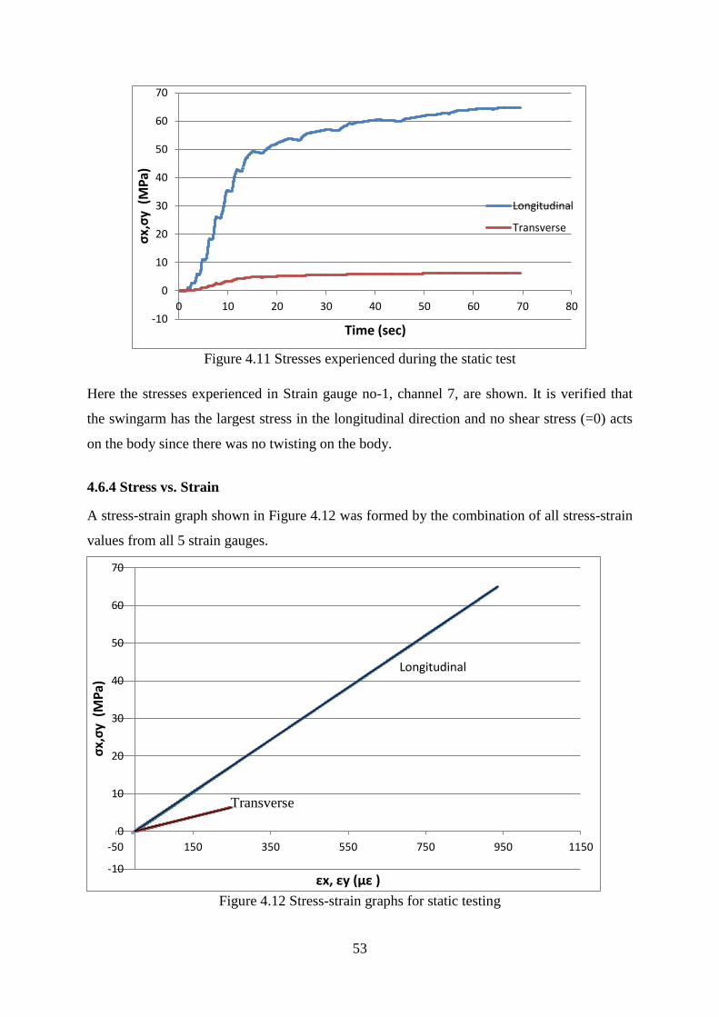
53
Figure 4.11 Stresses experienced during the static test
Here the stresses experienced in Strain gauge no-1, channel 7, are shown. It is verified that
the swingarm has the largest stress in the longitudinal direction and no shear stress (=0) acts
on the body since there was no twisting on the body.
4.6.4 Stress vs. Strain
A stress-strain graph shown in Figure 4.12 was formed by the combination of all stress-strain
values from all 5 strain gauges.
Figure 4.12 Stress-strain graphs for static testing
-10
0
10
20
30
40
50
60
70
0 10 20 30 40 50 60 70 80
σx,
σy
(M
Pa)
Time (sec)
Longitudinal
Transverse
-10
0
10
20
30
40
50
60
70
-50 150 350 550 750 950 1150
σx,
σy
(M
Pa)
εx, εy (με )
Longitudinal
Transverse

54
Here the strains experienced due to the stresses applied while statically testing the swingarm
is shown. A linear path is followed for the stress-strain curves in all directions. All points
where the gauges were placed exhibit linear elastic behaviour. The stress-strain curve can be
divided into two distinct deformation regions, which are the elastic deformation and the
plastic deformation. The elastic deformation is temporary and is fully recovered when the
load is removed. The plastic deformation is permanent and is not recovered when the load is
removed.
The line that is straight (Figure 4.12) shows the elastic deformation region. Within this region
if the load is removed the specimen would return to its original length. The slope of the curve
in this region (stress/strain) was identified as Young’s modulus. There was no record for
failure of the swingarm (as seen in graph) because the load applied to the arm was limited as
the swingarm test piece was needed for further testing in BST. Thus the plastic deformation
region is not show in the graph. The stress-strain equation based on the classical laminate
theory for composites was used (Eqn. 4.7). Using the equations the stresses ( )
were calculated.
The equations to determine stresses from strains (from graph) are given by:
For longitudinal stress,
σx = 0.0694 * εx (4.9)
For transverse stress,
σy = 0.0248 * εy (4.10)
Where, Stresses in MPa and
Strains in micro-strain (με)
4.7 Dynamic Test Results
In design situations, the number of stress cycles a part is designed to undergo is limited by the
life of the part. The maximum completely reversing cyclic stress that a material can withstand
for indefinite (or infinite) number of stress cycles is known as the fatigue strength or
endurance strength of the part material. When a part is subjected to cyclic stress it has been
observed that the failure of the part occurs after a number of stress reversals even if the
magnitude of the cyclic stress is below the material’s yield strength. Generally, higher the
cyclic stress, lesser number of reversals is needed for failure.

55
This section details that the applied load creates stresses below the endurance limit and thus
the body will undergo indefinite (or infinite) number of stress cycles. This validates that the
arm can successfully withstand the total load applied during a real-life test without failure.
The test was done for more than 1.2 million cycles as required by BST standards. After a
number of cycles the strains experienced by the swingarm reached a steady state as shown in
Figure 4.17. There was no failure to the swingarm during this dynamic test and this proves
that the swingarm can withstand a real-life test with infinite life.
Applied load: from eqn. A.3 & A.4.
Preloaded loading – 2470 N
Cyclic loading – 2365 N
4.7.1 Load vs. Time
The total load applied in each second is shown in Figure 4.13.
Figure 4.13 Effective load applied in one second
The loading consisted of a 2470 N static value, on which was superimposed a dynamic cyclic
load of 2365 N with a frequency of 3.5 cycles/second. The graph proves that the load during
each cycle was consistent since the test runs on the basis that the required total load is applied
throughout each test cycles.
0
500
1000
1500
2000
2500
3000
3500
4000
4500
5000
5500
0 0.2 0.4 0.6 0.8 1
Load
(N
)
Time (sec)
load
1 cycle
Preloading of 2470N
Cyclic loading of 2365 N

56
4.7.2 Transmission History
The longitudinal strain recorded with the NI DAQ system is shown in Figure 4.14. For better
visualization the last few cycles are shown [61].
Figure 4.14 Strain readings from the dynamic test
The trend line shows that a steady state was reached. These steady state values will be used
for further analysis. The number of cycles when steady state was reached is calculated by:
Number of cycles = time (sec) * Frequency
= 20790 cycles
Where Frequency = 3.5 cycles/second (from Appendix A.3)
Time = 5940 seconds
4.7.3 Strain in One Second
The strains experienced by the body in a second are shown in Figure 4.15.
-100
0
100
200
300
400
500
600
700
800
5935 5936 5937 5938 5939 5940 5941 5942 5943 5944 5945
stra
in (
με)
Time (sec)
strain 4
strain 0
strain 2
strain 3
strain 1

57
Figure 4.15 Effective strains in one second
Here the strains experienced in Strain gauge no-1, channel 7, are shown. The Longitudinal
strain has the highest value as expected. All strains values exhibits a cyclic path since a cyclic
load is applied as shown in Figure 4.15. The maximum and minimum longitudinal strain
(which is consistent) during each cycle along with the strain due to preloading and cyclic
loading is shown for better visualization of the effect of the respective loads on the arm. The
strain due to preloading from the initial value of 0 to εx-min is not shown on the graph because
its effect is only visible during the first cycle of the test. There is no shear strain (=0) acting
on the body.
4.7.4 Stresses in One Second
The stresses experienced by the body during the dynamic test in each second are shown in
Figure 4.16.
0
100
200
300
400
500
600
700
800
0 0.2 0.4 0.6 0.8 1
Stra
in (
με)
Time (sec)
Longitudinal
Shear
Transverse
strain due to cyclic loading
strain due to preloading
εx- min
εx- max

58
Figure 4.16 Stresses experienced in each second during the dynamic test
Here the stresses experienced in Strain gauge no-1, channel 7, are shown. All stress values
exhibit a cyclic path since a cyclic load is applied. A cyclic stress means when the stress
alternates between equal peak stresses during each cycle of operation. Cyclic stress over time
can be represented by a sinusoidal curve as shown. The maximum and minimum longitudinal
stress (which is consistent) during each cycle along with the stress due to preloading and
cyclic loading is shown for better visualization of the effect of the respective loads on the
arm.
The stress due to preloading from the initial value of 0 to σx-min is not shown on the graph
because its effect is only visible during the first cycle of the test. It is verified that the
swingarm has the largest stress in the longitudinal direction and no shear stress (=0) acts on
the body since there was no twisting on the body.
Some of the findings from the graphs are given below: (for longitudinal stress)
1. Stress range,
= max - min = 21.648 Mpa (4.11)
2. Alternating stress,
a = | max - min |/2 = 10.824 Mpa (4.12)
3. Mean stress,
0
10
20
30
40
50
60
0 0.2 0.4 0.6 0.8 1
σx,
σy
(M
Pa)
Time (sec)
Longitudinal
Shear
Transverse
σx max
σx min
Stress due to preloading
Stress due to cyclic loading

59
m = | max + min |/2 = 39.272 Mpa (4.13)
4.7.5 Stresses vs. Number of Cycles
The average stresses experienced by the body during the entire dynamic test are shown in
Figure 4.17.
Figure 4.17 Stresses experienced during the dynamic test
Fatigue design methodologies for metallic components have been traditionally based on the
stress-life approach [32] and this approach works well for designs involving long life. Here
the average stresses experienced in Strain gauge no-1, channel 7, are shown. At this point the
swingarm has the largest stress in the longitudinal direction. It has been observed that for
most of engineering materials, the rate of reduction of cyclic stress becomes negligible near
the vicinity of N = 106 and the slope of the stresses vs. number of cycles curve becomes more
or less horizontal. The fatigue strength of the arm dropped after a first few 10 000 cycles and
stabilized afterwards to infinite life. The steady state was reached after 20 000 cycles as
shown.
After 1.2 million cycles the swingarm was further tested and validated to be having infinite
life. Since the slope of the above curve is horizontal after certain cycles, if we keep the cyclic
stress value equal or less than the values of this test, the part will survive indefinitely (infinite
number of stress reversals). This proves that the applied load creates stresses below the
endurance limit and that the arm can successfully withstand the total load applied during a
real-life test without failure. No tests were conducted by applying higher loads to test the
0
5
10
15
20
25
30
35
40
45
0 10 100 1000 10 000 100 000 1 000000
1 200000
1 500000
σx,
σy
(M
Pa)
Number of stress cycles
Transverse
Longitudinal
Steady state Infinite life
Finite life

60
endurance limit of the swingarm since no higher loads are applied on the swingarm during its
life.
4.7.6 Stress vs. Strain
A stress-strain graph shown in Figure 4.18 was formed by the combination of all stress-strain
values from all 5 strain gauges.
Figure 4.18 Stress-strain graphs for dynamic testing
Here the strains experienced due to the stresses applied while dynamically testing the
swingarm is shown. The line that is straight (Figure 4.18) shows elastic deformation which
means if you stop pulling, the material will go back to its original size. The slope of the
stress-strain curve in the elastic deformation region is the modulus of elasticity, which is
known as Young's modulus. It represents the stiffness of the material or resistance to elastic
strain. The design of machines is based on component materials operating within this region.
Thus the plastic deformation region is not show in the graph because the component was
designed in such a way that the stresses applied to it during its operation are never beyond the
elastic deformation region.
The stress-strain equation based on the classical laminate theory for composites was used.
Using the equations the stresses ( ) were calculated. The equations to determine
stresses from strains (from graph) are given by:
y = 0.0694x
y = 0.0248x
-10
0
10
20
30
40
50
60
-100 100 300 500 700 900
σx,
σy
(MP
a)
εx,εy (μ ε)
Transverse
Longitudinal

61
For longitudinal stress,
σx = 0.0694 * εx
For transverse stress,
σy = 0.0248 * εy
Where, Stresses in MPa and
Strains in micro-strain (με)
The equations are the same in both static and dynamic tests (i.e. Eqn. 4.9 and Eqn. 4.10). The
results indicate a good correlation between the static and dynamic test to arrive at the same
equations.
4.8 Chapter Summary
The structure of this dissertation is such that chapter-specific summary and discussions have,
to a large extent, been included in the respective chapters. The results of the swingarm testing
were presented and discussed in this chapter.
Parameters that affect the final mechanical properties of composites such as orientation,
thickness and volume fraction were discussed with its effect on the current design of the
swingarm. The swingarm composite with maximum strength and stiffness in the shear and
transverse direction along with a good longitudinal stiffness was created using fibre
orientation of the different composite layers. It is also observed that strength and elasticity of
the material changes with thickness and volume fraction respectively. But the cost of
production will rise since more material is being used. A similar approach was carried out in
the design of the carbon fibre swingarm for a cost effective composite with maximum
strength and elasticity for its job.
The static test was conducted to analyse the fatigue strength of the arm, but there was no
record for any failure of the swingarm since the load was limited as the swingarm test piece
was needed for further testing in BST. The dynamic test was done to analyse the safety of the
swingarm to withstand a real-life test without failure with a factor of safety of two or more.
The test was conducted for 1.5 million cycles with the exact loading as a real-life test and
validated that the arm has infinite life at this particular loading since the applied load creates
stresses below the endurance limit and never beyond the elastic deformation region. No tests
were conducted by applying higher loads to test the endurance limit of the swingarm since no
higher loads are applied on the swingarm during its life.

62
Different aspects such as load, strain and stress were analysed with respect to time to show
the steady state of the system after a number of cycles. The results indicate a good correlation
between the static and dynamic test to arrive at the same equations for the stress vs. strain
curve. But there were no published results available, for the carbon fibre swingarm, in the
literature of stresses and strains for comparison and error analysis.
The test rig was the first of its kind for swingarm testing and has highlighted a number of
unique aspects of the rig such as variability of the loading using the eccentric mechanism was
discussed. The rig helped in understanding the real- life behaviour of a swingarm, especially
while going over bumps, in a laboratory. It was possible to study the damper effect of the arm
while replicating all degrees of freedom as in real-life. But the interaction between rider and
vehicle was not replicated. There is significant scope for further work on this topic by testing
other carbon fibre components, by applying higher loads and including more accurate
interaction between the rider and vehicle.

63
Chapter 5: Conclusions and Future Work
The chapter is structured as follows:
1. The overall conclusions of this work are stated.
2. Recommendations for further work are suggested.
5.1 Conclusions
A test rig was designed to experimentally validate a carbon fibre swingarm of a motorcycle.
The test rig replicated the suspension of a Ducati 1098. The model builds upon the work of
others, selecting and combining the advantages and remedying the disadvantages of previous
work. It was able to overcome the drawback of the Leyni test bench (used in previous
research studies in the literature) and apply variable loads for static and dynamic tests. The
rig was able to test swingarms with a preload of 2470 N and a superimposed dynamic load of
2364 N. The rig can vary the static and dynamic loads to any value required. The model was
designed using SolidWorks 2009 and most of the test rig components were made in house for
cost saving. The model was computationally very efficient and was able to count the number
of cycles performed while storing all the data concerned with load and strain, experienced by
the swingarm during the fatigue testing.
The swingarm test rig was designed to give an industrial answer as to whether the swingarm
will pass the BS code for fatigue test, before mass production of the swingarms. The test rig
was an excellent approximation of a real-life test. It can be used for a deeper analysis and for
further development of the component. Since no published results were available for
comparison and error analysis, the strain gauge results can be used to compare the designed
rig performance to the performance of other rigs else, they can be used for the future work
involving FEA.
The model was successfully used to benchmark the swingarm performance. The test rig using
static and dynamic loading proved that the swingarm can withstand a real-life test with
infinite life. There was no record for the failure of the swingarm during static testing since the
load was limited as the swingarm test piece was needed for further testing. And for dynamic
testing, it is validated that the body will undergo infinite number of stress cycles since the
applied load creates stresses below the endurance limit and never beyond the elastic

64
deformation region. The test rig was shown to be versatile, accurate and efficient, with
potential for future application. This research has shown the benefit of test rigs for testing
motorcycle components.
5.2 Recommendations for Further Work
1. A number of improvements to the test rig model are suggested, including:
a) An option to place the swingarm in different directions on the test rig so as to test
the swingarm for twist and torsional test.
b) A different crank mechanism that can adjust the offset from the centreline of the
gearbox which can enable the system to be easy to operate with the capability of
adjusting the loads in a simpler manner.
c) Eliminating some of the rose joints which would improve the accuracy of the
whole system.
d) An option to place different types of swingarms and other carbon fibre
components made at BST on the test rig for fatigue testing.
2. The static test should be conducted until failure and the stresses in the swingarm can
then be compared to the swingarm material strength to assess its durability.
3. Work can be carried out towards a new design of the test rig using hydraulic actuators
so that higher loads can be applied which can be useful while testing other types of
swingarms or carbon fibre components. The purpose is not to replace the current
testing machine, but to have better control over the machine and to apply higher loads
during the test. The hydraulic servos would eliminate the eccentric mechanism
therefore improved reliability and accuracy would be achieved using hydraulics.
4. It was difficult to quantify the actual value and direction of the human damping force
on road. Development of suitable instrumentation for this quantification is required.
5. The next step would be to develop an FE model of the swingarm and to compare the
results with the test results from this report. The FE model would act as a guide to
determine the stress points on the swingarm for further testing with strain gauges.
65
References
1 BlackStone Tek. Official Website, "www.blackstonetek.com". February 2013.
2 Grote K. Design of a Torsional Fatigue Testing Machine at BST. South Africa: Blackstone
Tek; 2008.
3 Mangaraju KV, Yogaraja V, Karthik M, Dora BK, Babu R, Venkatesan R. Kinematic and
Dynamic Analysis of Monoshock Rear Suspension. SAE Paper no: 2004-32-
0020/20044307; 2004.
4 Kharul RV, Pomaje SD. Effect of Human Damping on Two wheeler Fatigue Life and Its
Simulation on Two Poster Rig Using Passive Rider. SAE Paper no: 2001-26-0049; 2001.
5 Kumar MD. Redesign and Implementation of Motorcycle Rear Swingarm. ERES
International Journal of Mechanical, Vol. 1, No. 1; 2013.
6 Mangaraju KV, Govardan D, Chavan C, Babu R, Venkatesan R. Optimization of Damping
Characteristics for Two Wheelers. SAE Paper no: 2008-32-0068 / 20084768; 2008.
7 Meijaard JP, Popov AA. Multi-body Modelling and Analysis into the Non-linear
Behaviour of Modern Motorcycles. United Kingdom: School of Mechanical, Materials
and Manufacturing Engineering, University of Nottingham; 2006.
8 Leal MF, Borg JA, Butkewitsch S. Optimal Robust Design of Motorcycle Suspension
Systems. SAE Paper no: 2000-01-3216; 2000.
9 Ide R, Ogushi T, Sunayama Y, Kishita Y, Watanabe S. Estimating of Motorcycle Frame
Strength by Virtual Durability Test. SAE Paper no: 2009-32-0143/20097143; 2009.
10 Carfagni M, Pierini M, Caprioli D. Set Up and Validation for a Simulation of a Scooter
Confort Bench. SAE Paper no: 2001-01-1875/4273; 2001.
11 Risitano G, Scappaticci L, Grimaldi C, Mariani F. Analysis of the Structural Behavior of
Racing Motorcycle Swingarms. SAE Paper no: 2012-01-0207; 2012.
12 Piazza SD. Ducati Chassis Design: Simulation and Experiment Testing. Bologna, Italy:
Ducati motor holding S.P.A.
13 Cassani S, Mancuso A. Shape Optimization of a High Performance Motorbike Single
Sided Swingarm. SAE Paper no: 2005-01-0887; 2005.
14 Armentani E, Fusco S, Pirozzi M. Numerical Evaluation and Experimental Tests for a
Road Bike Swingarm. Italy: Department of Industrial Design and Management, University
of Napoli; 2007.
15 Dragoni E, Foresti F. Design of a Single Sided Composite Swingarm for Racing
Motorcycles. Switzerland: International Journal of Mateils & Product Technology, Vol 13,
Pages 411-420; 1998.
16 Bruderick M, Denton D, Shinedl M, Kiesel M. Carbon Fiber Composite Body Structures
For the 2003 Dodge Viper. DaimlerChrysler Corporation.
17 O’Dea N. Motorcycle Swingarm Redesigned in Carbon Composite. Reinforced Plastics,
55 (1), pp 38-41; 2011.
18 Gaiani S. Industrialization of an Aluminium Alloy Single Swingarm for Ducati Monster
S4 R. Development Trends of Motocycles ll, page 288-303.
19 Iwasaki H, Mizuta A, Hasegawa T, Yoshitake H. Development of a Magnesium

66
Swingarm for Motorcycles. SAE Paper no: 2004-32-0048 / 20044335; 2004.
20 Campbell FC. Structural Composite Materials, Introduction to Composite Materials. 2010.
21 Corum JM, Battiste RL, Liu KC, Ruggles MB. Basic Properties of Reference Cross ply
Carbon-Fiber Composite. United States: Lockheed Martin Energy Research Corp.; 2000.
22 Eastern Cape Development Corporation. An Overview of the Eastern Cape Automotive
Industry. South Africa 2005.
23 Ministry of Heavy Industries & Public Enterprises. Automotive Mission Plan 2006-2016.
New Delhi, India 2006.
24 Kharul R, Balakrishnan S, Singa AV, Patil MG. Methodology Adopted to Establish Rig
Correlation with Customer Usage for Two Wheelers. SAE Paper no: 2005-32-
0029/20056542; 2005.
25 Singanamalli A, Kharul R, Jayaram N, ora B, Anand R. Optimization of Frame Design
Through Virtual Simulation of Bump Test. SAE Paper no: 2004-32-0021/20044308; 2004.
26 Balakrishnan S, Muniyasamy K, Singanamalli AV, Kharul R, Jayaram N. Application of
Fatigue Life Prediction Techniques for Optimising the Motorcycle Center Stand. SAE
Paper no: 2004-32-0046/20044333; 2004.
27 Muniyasamy K, Kharul R, Jayaram N, Govindarajan R. Vibration Fatigue Analysis of
Motorcycle Front Fender. SAE Paper no: 2005-32-0030/20056543; 2005.
28 Kharul R, Balakrishnan S, Singanamalli AV, Dora KB. Development of Generic Load
Cases for Motorcycle Components for Design Optimisation. SAE Paper no: 2007-32-
0095/20076595; 2007.
29 Kharul R, Balakrishnan S, Karedla D, Shawn S. Virtual Testing and Correlation for a
Motorcycle Design. SAE Paper no: 2010-01-0925; 2010.
30 Balakrishnan S, Sasun C, Anoop P, Kharul R. Accurate Estimation of Time Histories for
Improved Durability Prediction Using Artificial Neural Networks. SAE Paper no: 2012-
01-0023.
31 Pawar PR, Karanth NV. Effect of Disc Brake and Drum Brake on the Durability of Front
Shock Absorber Tube of a Motorcycle. SAE Paper No: 2003-26-0031; 2003.
32 Lin KY, Chang JM, Wu JH, Chang CH, Chang SH, Hwang JR, Fung CP. Durability
Assessments of Motorcycle Handlebars. SAE Paper no: 2005-01-0801; 2005.
33 Kharul R, Patil MG, Balakrishnan S, Risam GS. Methodology for Accelerated Vibration
Durability Test on Electrodynamic Shaker. SAE Paper no: 2006-32-0081 / 20066581;
2006.
34 Michiue M, Kawasaki T, Nishio K, Sugiura H, Inamura F, Morikawa M. Prediction of
Vibration Fatigue Life for Motorcycle Exhaust Systems. SAE Paper no: 2011-32-
0642/20119642; 2011.
35 Muthuveerappan G, Manoj V, Gopinath K. Development of a Power Re-Circulating Gear
Test Rig. Chennai, India: Dept. of Mechanical Enginnering, IIT Madras.
36 Crump D, Dulieu M, Savage J. Design and Commission of an Experimental Test Rig to
Apply a Full-Scale Pressure Load on Composite Sandwich Panels Representative of
Aircraft Secondary Structure. Measurement Science and Technology, 21 (1), pp 1-6; 2010.
37 Ismail K, Kadambi R, Thomas S. Development and Implementation of Test Rig setup for
Integrated Centre Panel. India: M.S.Ramaiah School of Advanced Studies; 2001.
38 Kumar S, Kundra TK, Modak SV. Model Updating Studies on a Two Wheeler Chassis.
SAE Paper no:2007-01-2353; 2007.
39 Carroll P, Carver S. Factors in the Mechanical Design of Motorcycle Laboratory Test

67
Systems. SAE Paper no: 2001-01-1879/4296; 2001.
40 Maurizio C. Topological Optimization of Side Plates For Rear Swingarm of Mv Agusta
F4 1000 My ’10. Cagiva Research Center; 2010.
41 Sato S, Sunayama Y, Sakamoto Y. Radiation Noise Analysis for Electric Scooter Swing-
arm. SAE Paper no: 2011-32-0650/20119650; 2011.
42 Ardiri D, Cammarata A, Sinatra R. Simulation of Roller Test Bench for Fatigue
Validation of a Scooter Frame. Italy: Piaggio Brand Unit Vehicle Mechanical System &
CAE.
43 Stefano V, Simone P. Structural Optimization of the Rear Swingarm of Ducati
HyperMotard. Berlin, Germany: 1st European HyperWorks Technology Conference;
2007.
44 University of the Witwatersrand. Guidelines for Design Reports, MECN2009 Notes.
South Africa 2011.
45 Zoerb GC. Strain Gage Instrumentation for Power Measurement. United States: South
Dakota State College.
46 National Instruments Corporation. Load and Pressure Measurements, www.ni.com/white-
paper/7138/en.. February 2013.
47 New Jersey Institute of Technology, Department of Engineering Technology. Design for
Cyclic Loading, MET 301. United States 2013.
48 Bradley E. Reliability Engineering Course notes, MECN 7001. South Africa: University
of the Witwatersrand; 2012.
49 Bryan H. Engineering Composite Materials. London, United Kingdom: The Institute of
Materials; 1999.
50 University of the Witwatersrand. Mechanics of Composite Materials, MECN4003 Notes.
South Africa.
51 Zipp Speed Weaponry. Woven Carbon Vs. Unidirectional, "www.zipp.com". United
States July 2013.
52 Oribi Manufacturing. Uni-Directional vs Woven, "www.oribimanufacturing.com". United
States July 2013.
53 Adis A, Ujjal KS. Simulating a Tensile Test of a Carbon Fibre Composite Test Specimen
in ABAQUS. Sweden: University of Skovde.
54 Department of Defence. Polymer Matrix Composites; Materials Usage, Design and
Analysis. United States 1997.
55 Toray Carbon Fibers. Toray Data Sheet: "www.toraycfa.com" & "www.torayca.com".
Japan February 2013.
56 TenCate Advanced Composites. Technical Data for RS-36 Resin System:
"www.tencate.com". United States July 2013.
57 Tomblin J, Sherraden J, Seneviratne W, Raju KS. A–Basis and B–Basis Design
Allowables for Epoxy Based Prepreg. Advanced General Aviation Transport Experiments
(AGATE); 2002.
58 Tienie VS. Short Course on Filamentary Composite Materials. South Africa: University of
Pretoria; 1998.
59 Tiwari N. Mechanics of Laminated Composite Structures. Kanpur, India: Indian Institute
of Technology.
60 Calard V. Formulas and Equations for the Classical Laminate Theory. 2011.

68
61 Socie D. Fatigue Analysis Techniques. United States: University of Illinois.
62 Fibro Springs. Round Wire Compression Spring, "www.fibro.de". February 2013.
63 Mahadevan K, Reddy K. Design Data Hand Book. India: CBS Publishers and
Distributors; 2002.
64 Budynas RG, Shigley JE, Nisbett JK. Shigley's Mechanical Engineering Design.
McGraw−Hill; 2008.
65 Einstein College of Engineering. Course Notes on Design of Machine Elements. Tamil
Nadu, India.
66 Koyo Bearings. Ball and Roller Bearings, "www.koyousa.com". United States February
2013.
67 National Instruments Corporation. Strain Gauge Measurements, "www.ni.com/white-
paper/3642/en". Ferbruary 2013.
68 Micro-Measurements. Shunt Calibration of Strain Gage Instrumentation, www.micro-
measurements.com. February 2013.
69 Vozkova P. Elastic Modulus FEM Modelling of the Layered Woven Composite Material.
Czech Republic: Technical University of Liberec.

69
Appendix A
A.1 Cost of Machined Components
Table A.1 The cost of machined components within the factory
Components machined Material Qty.
(kg)
Cost
(Inc.
VAT)
(per kg)
Total cost
(Inc. VAT)
(R)
Eccentric mechanism components (only for electrical test rig)
Eccentric shaft En19 1 33 33
Eccentric bolt En19 0.5 33 16.5
Con-rod En19 2 33 66
Angle plates (2 numbers) En19 14 33 462
Hexagonal bolt En19 1 33 33
Eccentric hub and its shaft (2 numbers) En19 8 33 264
Essential nuts and bolts
250
Total cost of machined components (only for electrical test rig) 1125
Swingarm attachment components (common for electrical and hydraulic)
Angle plates (2 numbers) En19 12 33 396
Swingarm pivot En19 3.5 33 115.5
Rocker arm Aluminium 1 60 60
Wheel hub Aluminium 1 60 60
The two rods Aluminium 1 60 60
Essential nuts and bolts 250
Slider and spring mechanism components (common for electrical and
hydraulic)
Slider rail En19 0.5 33 16.5
Slider base Aluminium 2.5 60 150
Sliding arm En19 1 33 33
Essential nuts and bolts
120
Spring housing Aluminium 4 60 240
Total cost of machined components (common for electrical and hydraulic) 1501

70
The cost of components purchased which are common for electric and hydraulic test rig is
given below.
Table A.2 Cost of components purchased
Components and specifications purchased QTY Price (Inc.
VAT)
Total (R)
(Inc. VAT)
Static test rig components (common for electrical and hydraulic)
Single sided hydraulic Ram 1 950 950
Chain 1 116.28 116.28
Dynamic test rig components (common for electrical and hydraulic)
Ohlin’s springs 2 494 988
2 plummer blocks for angle plates 2 240 480
Linear way for sliding mechanism 1 245 245
IKO Rod End bearing (rose joint) 3 263 789
Base plate 1 6775 6775
Total cost of purchased components (R) 10343
A.2 Load Design
Given data
Acceleration due to gravity, g = 9.810 m/s2
Motorcycle weight, Wb = 2158 N
Weight of rider and passenger, Wr = 1960 N
The maximum load to be reached while testing, F = 5900 N [18] (Appendix E, test
factor (Kr) of 1.431)
Equations and calculations
The cyclic load,
Fc = F – Wr = 3940 N (A.1)
Total preload,
Fp = Wb + Wr = 4118 N (A.2)
Real wheel loads, taking (on rear wheel) 60 % / 40% (one front wheel) split: [14]
Rear wheel cyclic load,

71
Frc = 0.6*Fc = 241 kg = 2364 N (A.3)
Rear wheel total preload,
Frp = 0.6*Fp = 251 kg = 2470 N (A.4)
Maximum load on the rear wheel is,
Fmax-r = Frc + Frp = 4835 N (A.5)
A.3 Spring Design
A spring is an elastic member, which deflects, or distorts under the action of load and regains
its original shape after the load is removed. The factor of safety of a selected spring is
calculated and it is used for this research if it is greater than one.
Function of the spring.
1. To measure forces in spring balance, meters and engine indicators.
2. To store energy.
Given data
Spring material: spring steel Class C
Spring type no : 241.02.44.200 by Fibro springs [62]
Hard-drawn wire
Round wire compression spring
Figure A.1 Dimensions of a spring
Dh = diameter of guide sleeve = 44 mm
Dm = mean coil diameter = 34 mm

72
Dd = coil diameter = 8 mm
L0 = free length of spring = 200 mm
K = the load required per unit deflection of the spring, spring rate = 62700 N/m
Na = number of active coils = 17 turns
Young’s modulus, E = 2.07E+11 N/m2
Shear modulus, G = 8.10E+10 N/m2
α= 0.5, since spring supported between flat parallel surfaces
Density, ρ= 7850 kg/m3
Fatigue strength in reversed shear, Ssa = 398 MPa
Ultimate strength in shear, Ssm = 534 MPa
Minimum load cycles = 1.20E+06 cycles
Speed of shaft, N = 210 rpm
Torsional frequency, f = 3.5 cycles/second
Equations and calculations
Forces acting on spring
Maximum force, from Eqn. A.3 and A.4
Fmax = 2364 + 2470 ≈ 5000N
Minimum force, (before preloading)
Fmin = 0 N
Spring index = mean coil diameter / coil diameter = 4
The maximum shear stress in the spring associated with the maximum force is given by [63]
τmax
*Fmax= 1163 MPa (A.6)
Where W is the Wahl correction factor
W =
= 1.380 (A.7)
The total number of spring coils is equal to the active coils in the spring interior plus the 2
coils at the spring ends,
nf = na + 2 = 19 (A.8)
The solid length of the spring is length of a spring under the maximum compression,
Ls = (Nf -0.75) d = 146 mm (A.9)
To determine if spring is stable:
Free length, [64]

73
*√
( )
= 176.540 (A.10)
OK since it has a guide to travel in.
Ultimate tensile strength of spring,
Sut =
= 1201 MPa (A.11)
Where A = 1783 MPa.mm2
M= 0.190
The spring mass, M can be found by finding the spring volume and multiplying by its
material density,
M = ρ * Vol. = ρ * (Lwire*
* d2) (A.12)
= 0.717 kg
Where Lwire = π*d*Ns
The natural frequency of the spring,
fn = 0.25*√
= 74 Hz (A.13)
To determine the safety factor of spring:
Yield strength in shear,
Sse =
= 711.170 MPa (A.14)
Stress components are given by
τm = w* 8* Fm*C / π*d2 = 581 MPa
τa = w* 8* Fa*C / π*d2 = 581 MPa (A.15)
Where Fa = (Fmax – Fmin) /2
Fm = (Fmax+ Fmin)/2
The factor of safety
Sf = Sse/ τa = 1.2 (A.16)
OK, since its Sf is greater than 1

74
A.4 Motor Design
The electric motor (Figure A.2) provides the required power to the whole dynamic test rig at
a given frequency. A gear system is attached to the motor to provide the required torque. This
component can be a significant contributor to the cost of the whole test system and is
therefore worth the time to properly evaluate it instead of buying an overrated system.
Figure A.2 Eccentric mechanism components and the electric motor
Equations and calculations Rotating forces:
Maximum rotating force, from Eqn. A.3
Fmax1 ≈ 2500 N
Minimum rotating force, (when motor is not running)
Fmin1 = 0 N
Eccentric radius:
Maximum eccentric radius needed
Fmax1 /K = 0.040 m
Minimum eccentric radius needed
Fmin1 /K = 0 m
Where K = spring rate
Torque needed for transmission:
Maximum torque that needs to be transmitted
Fmax1*Max eccentric = 99.7 Nm
Minimum torque that needs to be transmitted

75
Fmin1*Min eccentric = 0 Nm
Power needed by motor =
Max torque * f *2π / 1000 = 2.190 kW (A.17)
Motor details:
Power, P = 4 kW, OK, since chosen power is greater.
Rated speed =1400 RPM
Rated Frequency, Rf = 23.334 Hz
I = Rf / f = 6.700
Torque,
(P*1000) / (Rf *2π) = 27.3 Nm (A.18)
A.5 Eccentric Bolt Design
The eccentric bolt (Figure A.3) attaches the eccentric shaft to the eccentric hub. Since the bolt
takes a large amount of stress during a test, it is designed with a factor of safety greater than
one.
Figure A.3 Eccentric system of the test rig
Given data
No of bolts = 2
Material – EN19
Yield stress, Sy = 480 MPa
Tensile stress, Sut = 690 MPa

76
Assume bolt diameter, Das= 16 mm
Assume safety factor, Sf = 1.3
Equations and calculations
Endurance limit,
Se'= 0.504 * Sut = 347.760 MPa (A.19)
Forces acting on bolts:
Max shear force experienced on each bolt
Fmax2 = Fmax /2 = 2500 N
Min shear force experienced on each bolt
Fmin2 = Fmin/2 = 0 N
Adjustment of the Endurance Limit,
Surface Condition (Ka): Assume machined,
Ka =a* (Sut) b
= 0.798 (A.20)
Where a = 4.51MPa
b = -0.265
Size (Kb):
Kb = 1.24*(0.37*Das)-0.107
= 1.025 (A.21)
Load (Kc) = 1
Temperature (Kd): Assume operating temperature, t = 25 °C
Kd =0.975+0.000432*t-(1.15)*10-6
*t2+ (1.04)*10
-9*t
3 (A.22)
= 0.985
Reliability (Ke): Assume 90% reliable = 0.897
Miscellaneous (Kf): Assumed reversed bending = 1
Real-World Allowable Cyclic Stress,
Se = ka * kb * Kc * kd * ke * kf * Se' (A.23)
= 251.310 MPa
Bending moment,
M = (Fmax2 *length to disk) / 1000 = 75 Nm (A.24)
Where, length to disk = 30 mm
Diameter of bolt,
d = [
(1/3)
= 15.810 mm (A.25)
OK, since chosen diameter is greater.

77
A.6 Eccentric Shaft Design
Similar to the eccentric bolt, the eccentric shaft (Figure A.4) connects the two eccentric hubs
together and the double row angular contact ball bearing’s inner race fits along the shaft and
thus it is designed with a factor of safety greater than one.
Figure A.4 Eccentric shaft and its components
Given data
Material – EN19
Yield stress, Sy = 480 MPa
Tensile stress, Sut = 690 MPa
Assume safety factor, Sf = 5
Shaft diameter, d= 45 mm
D = d/.75 = 60 mm
r = D/20 = 3 mm
Theoretical stress-concentration-factor for bending, Kt = 1.750
Theoretical stress-concentration-factor for torsion, Kts = 1.5
Equations and calculation
Torque transmitted to shaft,
Torque of motor * I = 181.9 Nm (A.26)
τmax= 181.9 Nm
τmin= -189.9 Nm
Reversed Bending moment transmitted to shaft = 2M = 150 Nm
Mmax = 150 Nm
Mmin = -150 Nm

78
Endurance limit,
Se'= 0.504 * Sut = 347.760 MPa
Adjustment of the Endurance Limit,
Surface Condition (Ka): Assume ground,
Ka =a* (Sut) b
= 0.906
Where a = 1.580 MPa
b = -0.085
Size (Kb):
Kb = 1.24*(0.37*d)-0.107
= 0.825
Load (Kc) = 1
Temperature (Kd): Assume operating temperature, t = 25 °C
Kd =0.975+0.000432*t-(1.15)*10-6
*t2+ (1.04)*10
-9*t
3
= 0.985
Reliability (Ke): Assume 90% reliable = 0.897
Miscellaneous (Kf): Assumed reversed bending = 1
Real-World Allowable Cyclic Stress,
Se = ka * kb * Kc * kd * ke * kf * Se'
= 229.840 MPa
Stress-concentration factors:
Fatigue stress-concentration factor for bending,
K f =
( )
√
√
= 1.590 (A.27)
Fatigue stress-concentration factor for torsion,
Kfs =
( )
√
√
= 1.390 (A.28)
Where, stress concentration at shoulder
√ = 139/Sut = 0.201
Shaft stresses:
Maximum axial stresses,
σmax = (
)
= 26.680 MPa (A.29)

79
Minimum axial stresses,
σmin = (
)
= - 26.680 MPa (A.30)
Maximum torsional stresses,
τmax = (
)
= 14.150 MPa (A.31)
Minimum torsional stresses,
τmin = (
)
= - 14.150 MPa (A.32)
Midrange axial stresses,
m = ( max + min)/2 = 26.680 MPa (A.33)
Alternating axial stresses,
a = | max - min |/2 = 0 (A.34)
Midrange torsional stresses,
τm = (τmax + τmin)/2 = 14.150 MPa (A.35)
Alternating torsional stresses,
τa = |τmax −τmin|/2 = 0 (A.36)
Diameter of shaft [65]
d= [
*{
+
}] (1/3)
(A.37)
= 41.520 mm
OK, since chosen diameter is greater.
A.7 Thread for the Hexagonal Bolt Design
The hexagonal bolt attaches the spring housing to the eccentric mechanism as shown in
Figure A.2 through the thread for the hexagonal bolt (Figure A.5). The design for this thread
ensures less chance for thread cracks and could lead to higher reliability in the entire test rig.

80
Figure A.5 Hexagonal bolt and its components
Given data
Material – EN19
Yield stress, Sy = 480 MPa
Maximum force (from Eqn. A.3 and A.4), Fmax = 5000 N
Assume: Diameter of rod on which thread lies, d = 20 mm
Pitch of thread, p = 1.5 mm
Length of thread, L = 25 mm
Equations and calculation
The area under which the stress acts A,
Π*d * L = 1570 mm2
(A.38)
Load capacity of bolt
Fa = C*(A) 1.48
= 23816 N (A.39)
Where C = 0.7 for alloy steel
Shear stress on thread
Fmax/A = 3.184 N/mm2
(A.40)
Safety factor,
Sf = Sy/shear stress = 150 (A.41)
OK, since its Sf is greater than 1

81
A.8 Bearing Design
Bearings enhance the functionality of any machinery and help to save energy. Bearings do
their work silently, in tough environments, hidden in machinery where they can't be seen. The
purpose of a bearing is to reduce friction, most often on a rotating shaft. The design for these
crucial components ensures fewer chances for failures.
A.8.1 Bearing Over the Eccentric Shaft Design
The double row angular contact ball bearing has its inner and outer race along the eccentric
rotating shaft and the con-rod respectively as shown in Figure A.4. Maximum load during the
dynamic test on the arm is 4835 N (Equation A.5). Thus 5000 N is used for calculations to
include a factor of safety greater than one.
Given data
Assume bearing is a double row angular contact ball bearing [66]
Inner diameter, d = 40 mm
Outer diameter, D = 85 mm
Specific capacity, C = 45400N
Basic static load rating, C0 = 51400 N
Speed of shaft, N = 210 RPM
Figure A.6 Dimensions of a double row angular contact ball bearing
Equations and calculation
Forces acting on bearing
Maximum force, from Eqn. A.5
Fmax ≈ 5000N
Minimum force, from Eqn. A.3

82
Fmin ≈ 2500 N
The constant mean load for a period of fluctuating loads is,
Fm = (Fmin + 2 Fmax)/2 = 4166.6 N
Radial force,
Fr = Fm = 4166.6 N
Axial force,
Fa = 0 N
Life in millions of revolutions,
Ln = (C/F) 3
= 1293.601 millions of revolutions (A.42)
Life in working hours,
Lh =
= 102666.7 hours = 11.720 yrs. (A.43)
OK since the bearing will last long enough.
A.8.2 Bearing Reactions
The 3 bearings which react against the force and friction on the rotation shaft are shown in
Figure A.2. The reactions of each bearing are calculated and the bearing with more load
acting on it is designed. Similar bearings will be used for all 3 plummer blocks to make the
system more reliable.
Figure A.7 Bearing reactions
Forces acting:
Ra + Rb + Rc = F = 5000 N
At 1: 0.142 F = 0.256 Rb + 0.352Rc

83
At F: 0.142 Ra = 0.114 Rb + 0.21 Rc
At 2: 0.256 Ra - 0.096 Rc = 0.114 F
At 3: 0.352 Ra +0.096 Rb = 0.011 F
Solving,
Ra = 1547.690 N, acting on the bearing 1
Rb = 3971 N, acting on the bearing 2
Rc = -518.690 N, acting on the bearing 3 in reverse direction as shown.
A.8.3 Bearing-2 Design
Since similar plummer blocks consisting of similar bearings are used in the test rig, it would
be optimum to design bearing 2 since there is more load acting on it as in Figure A.7.
Given data
Assume bearing is a deep groove ball bearing
Inner diameter, d = 30 mm
Outer diameter, D = 72 mm
Specific capacity, C = 26700 N
Basic static load rating, C0 = 15000 N
Speed of shaft, N = 210 RPM
Figure A.8 Dimensions of a deep groove ball bearing
Equations and calculation Forces acting on bearing
Radial force, Fr = Rb = 3971 N
Axial force, Fa = 0 N
Life in millions of revolutions,
Ln = (C/F) 3
= 303.972 millions of revolutions

84
Life in working hours,
Lh =
= 24124.790 hours = 2.754 yrs.
OK since the bearing will last long enough.

85
Appendix B
B.1 Strain Gauge Calibration
Fatigue test loads
Rear wheel cyclic load, Frc = 2364 N = 241 kg
Rear wheel total preload, Frp = 2470.9 N = 251.9 kg
Strain gauge equipment description
Equipment: National Instruments SCXI-1000 chassis, SCXI-1600 control card, SCXI-1521B
universal card, SCXI-1317 module
Features of strain gauges used:
Resistance = 119.8 ohm
FG = gauge factor of strain gauge = 2.12
Quarter-bridge circuit with a single active gauge.
Strain Gauge Method
Sample rate: 100 Hz
Low pass filter: 10 Hz
Calibration
The gauges were extremely stable.
Table B.1 Strain gauge calibration chart
As seen the % error was less than 2% and thus accepted.

86
B.2 Load Cell Calibration
Load cell calibration Equipment Description
Equipment: National Instruments SCXI-1000 chassis, SCXI-1600 control card, SCXI-1521B
universal card, SCXI-1317 module, load cell.
Loading and unloading of 350 kg was done by using weights.
Load cell wiring
EX + blue
EX - yellow
CH + red
CH - green
Load Cell Dead Weight Calibration
Table B.2 Load cell calibration data
Mass Load Voltage Mass Load Voltage
[kg] [N] [v] [kg] [N] [v]
0 0.00 -3.20E-04 325 3.18E+03 -1.62E-03
25 2.45E+02 -4.20E-04 300 2.94E+03 -1.52E-03
50 4.90E+02 -5.20E-04 275 2.69E+03 -1.42E-03
75 7.34E+02 -6.10E-04 250 2.45E+03 -1.32E-03
100 9.79E+02 -7.10E-04 225 2.20E+03 -1.22E-03
125 1.22E+03 -8.10E-04 200 1.96E+03 -1.12E-03
150 1.47E+03 -9.10E-04 175 1.71E+03 -1.02E-03
175 1.71E+03 -1.01E-03 150 1.47E+03 -9.20E-04
200 1.96E+03 -1.12E-03 125 1.22E+03 -8.20E-04
225 2.20E+03 -1.21E-03 100 9.79E+02 -7.20E-04
250 2.45E+03 -1.31E-03 75 7.34E+02 -6.20E-04
275 2.69E+03 -1.42E-03 50 4.90E+02 -5.30E-04
300 2.94E+03 -1.51E-03 25 2.45E+02 -4.30E-04
325 3.18E+03 -1.61E-03 0 0.00 -3.30E-04
350 3426.5 -1.72E-03
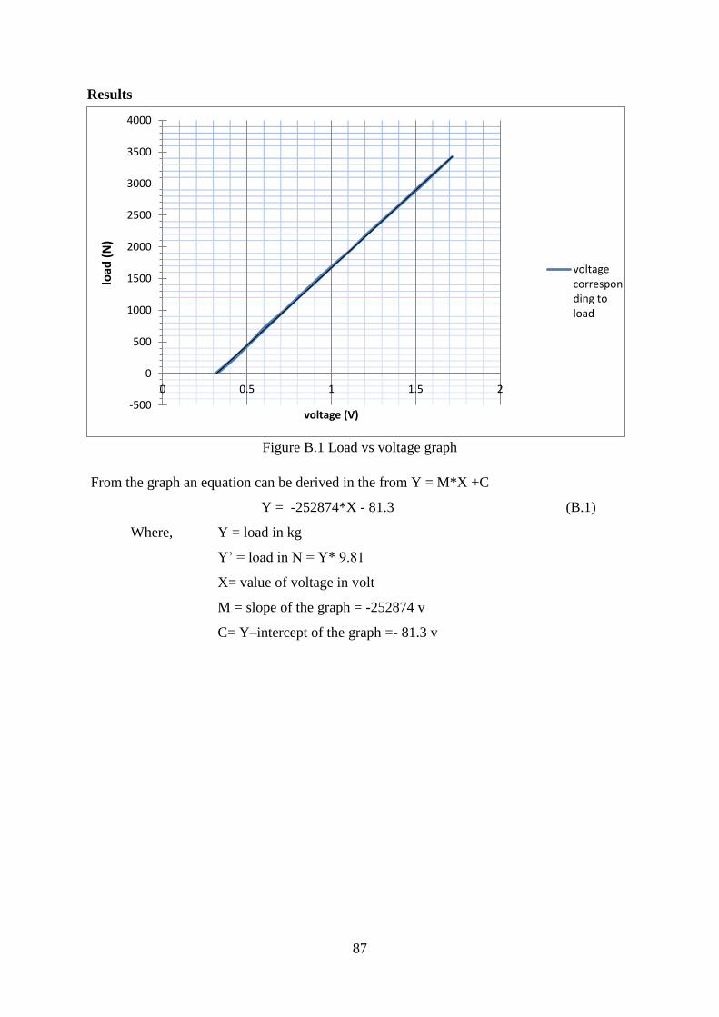
87
Results
Figure B.1 Load vs voltage graph
From the graph an equation can be derived in the from Y = M*X +C
Y = -252874*X - 81.3 (B.1)
Where, Y = load in kg
Y’ = load in N = Y* 9.81
X= value of voltage in volt
M = slope of the graph = -252874 v
C= Y–intercept of the graph =- 81.3 v
-500
0
500
1000
1500
2000
2500
3000
3500
4000
0 0.5 1 1.5 2
load
(N
)
voltage (V)
voltagecorresponding toload

88
B.3 Equations for Strain Gauge Measurements
To simplify the equations and account for unbalanced bridges in the non-strained state, let us
introduce the ratio Vr: [67]
Vr = (VO strained– V0 unstrainedVEX (B.2)
Where VO (strained) = measured output voltage when strained
VO (unstrained) = initial, unstrained output voltage
VEX = excitation voltage
Strain before correction takes the lead resistance in to consideration and is given by the
equation:
ε =
( )
(B.3)
Where RG = nominal resistance value of strain gauge
GF = gauge factor of strain gauge
RL = lead resistance
The corrected strain for a quarter-bridge circuit, with a single active gauge at any different
strain level can be calculated from: [68]
ε =
( ) (B.4)
Where ε = corrected strain
εs = calibration strain
εi = indicated strain

89
Appendix C
C.1 Young’s Modulus, Volume Fraction, the Thickness and the Poisson’s
Ratio of Lamina
Equations used
The rule of mixture model will be selected for the analysis in this research.
1. According to the rule of mixture model [58] [20], if an axial load is applied in the
longitudinal direction it will be shared by the fibre and the matrix, therefore
longitudinal modulus is given by:
E1= Ef*Vf + Em*Vm (C.1)
Maximum stiffness is obtained when the stress is applied parallel to the layers.
2. For the transverse modulus, a load is assumed to be applied at right angles to the fibre
direction. The simplified equation for transverse stiffness is:
(C.2)
When the layers are orientated transverse to the applied stress, the effective modulus
is lower. Generally the matrix dominated properties of composites material are
usually much lower in magnitude than the fibre dominated properties.
3. The major Poisson’s ratio refers to the case where a load applied in the fibre direction
results in a strain in the fibre direction and a Poisson’s contraction transverse to the
fibre direction. The major Poisson’s ratio is defined as:
υ12 = υf*Vf + υm*Vm (C.3)
4. For a composite with n layers of fibre with a known areal mass, the total thickness is
given by:
Tc1 = n *
(C.4)
Total no of lamina, n= n1+n2 = 12
5. Volume fraction of each material is the ratio of the thickness contribution of that
material to the total thickness.
Vc1 =
(C.5)
fffm
fm
EVVE
EEE
)1(2

90
C.2 New Stiffness Values According to the Orientation of Ply in Tension
and Compression
C.2.1 Equations Used
The elastic constants for a lamina at an orientation to the reference axes were simplified to
give the following equations. [49] [69]
1. The longitudinal modulus could be defined as
Ex = [
(
- 2
) * sin
2 θ * cos
2 θ +
]-1
(C.7)
2. Similarly transverse modulus could be defined as
Ey = [
(
- 2
) * sin
2 θ * cos
2 θ +
]-1
(C.8)
3. The shear modulus was defined as
Gxy = [ (
+
+4
)*sin
2 θ*cos
2 θ+
( )]-1
(C.9)
4. Finally the Poisson’s ratio was defined as
vxy = Ex *[
( ) - (
+
)*sin
2 θ*cos
2 θ)] (C.10)
C.2.2 Variation of Elastic Constants with Fibre Orientation
Using the above equations and the given data from Table 3.3 for the Toray 700G which is in
+450/-45
0 orientation, the following conclusions were formulated.
For tension
The longitudinal and transverse modulus was varied with fibre orientation angle from 00 to
900 [21]. The results are shown in Figure C.1.

91
Figure C.1 Variations of Young’s modulus for Toray 700G with orientation
The highest and lowest values of E1 and E2 are same and at 450 the value of E1 and E2 will
be the same. The stiffness of the composite falls rapidly as the loading direction shifts away
from the fibre axis, the effect being marked more, if the stiffness of the reinforcing fibre is
higher.
The shear modulus was varied with fibre orientation angle from 00 to 90
0. The results are
shown in Figure C.2.
Figure C.2 Variations of shear modulus for Toray 700G with orientation
Since the variation of shear modulus is less sensitive compared to others, it is shown in a
different graph for better visibility of the effect. The shear stiffness of the composite is less
sensitive to the matrix characteristics as angle increases from 00 to 45
0, being largely
controlled by the fibre rigidity. The shear modulus is a maximum however in a direction at
45° to the fibre axis thus the lamina will resist torsion.
0
20
40
60
80
100
120
140
160
0 15 30 45 60 75 90
E1,E
2 (
GPA
)
Angle (deg)
E1
E2
0
1
2
3
4
5
6
7
8
9
10
0 15 30 45 60 75 90
G (
GPA
)
Angle (deg)
G

92
The Poisson’s ratio was varied with fibre orientation angle from 00 to 90
0. The results are
shown in Figure C.3.
Figure C.3 Variations of Poisson’s ratio for Toray 700G with orientation
It is noted that the Poisson’s ratio of composites can be relatively large in comparison to a
normal isotropic material. This means firstly, that the deformations associated with Poisson’s
expansion/contraction can be large and secondly, that if these deformations are restrained in
any ways, the associated stresses can be quite high.
For compression
Figure C.4 Variations of elastic constants for Toray 700G with orientation
The Figures indicate that good properties in a particular direction come at the expense of poor
properties in another direction. Note that for tension and compression, fibre behaviour
0
0.05
0.1
0.15
0.2
0.25
0.3
0.35
0.4
0 15 30 45 60 75 90
Po
isso
n’s
rat
io (
υ)
Angle (deg)
v
0
10
20
30
40
50
60
70
80
90
100
110
120
130
140
0 15 30 45 60 75 90
E1,E
2, G
(G
Pa)
& υ
(*1
00
)
Angle (deg)
E1
E2
v*100
g

93
dominates the O/900 behaviour, while matrix behaviour dominates the +45
0 direction. These
roles are reversed in the shear case, the +450 behaviour is fibre dominated. ± 45
0 is the ideal
fibre angle to resist pure torsion. The transverse modulus is matrix dominated and tends to be
very low in comparison to the fibre dominated longitudinal modulus. Hence a sensible
approach to design would be to ensure that transverse stresses are minimised.
C.3 Effective Elastic Constants of the Swingarm for the 12 Layers
Equation used
For simple hybrids consisting of unidirectional plies or mixed, aligned fibre tows, a technique
to estimate the effective elastic constants as a function of the volume fraction of the body is
done with the following equation. [49] The Young’s modulus and shear modulus of most
laminate hybrids are predicted satisfactorily by this method. Equation C.1 becomes:
Ehybrid= EA*VA + EB*VB (C.11)
Ghybrid= GA*VA + GB*VB (C.12)
Where EA/GA and EB/GB are the moduli of the individual components and VA and VB
are the volume fractions of the components. As in the case of a simple composite,
VA + VB = 1.

94
Appendix D
D.1 Effect of Thickness
The thickness is varied by changing the number of laminae in each material with the ratio of
1:1 (700s: 700G) and the new effective stiffness was calculated. The results were then
formulated in to a graph to show the effect of thickness on elastic constants.
Results
Table D.1 Effect of thickness on elastic constants
No of
layers
Thic
kness
Thic
kness
Thic
kness
Volume
fraction
Volume
fraction
Elastic
modulus
Elastic
modulus
Shear
modulus
Total t700S t700G Total t700S t700G E11 E22 G
2 0.41 0.52 0.92 0.441 0.559 58.57 11.8 6.99
4 0.81 1.03 1.84 0.441 0.559 58.57 11.8 6.99
6 1.22 1.55 2.77 0.441 0.559 58.57 11.8 6.99
8 1.63 2.06 3.69 0.441 0.559 58.57 11.8 6.99
10 2.03 2.58 4.61 0.441 0.559 58.57 11.8 6.99
12 2.44 3.09 5.53 0.441 0.559 58.57 11.8 6.99
14 2.85 3.61 6.45 0.441 0.559 58.57 11.8 6.99
16 3.25 4.12 7.37 0.441 0.559 58.57 11.8 6.99
18 3.66 4.64 8.3 0.441 0.559 58.57 11.8 6.99
20 4.07 5.15 9.22 0.441 0.559 58.57 11.8 6.99
The variations of effective elastic constants with thickness of the composite are shown in
Figure D.1

95
Figure D.1 Variations of effective elastic constants with thickness of composite
The effective longitudinal modulus is higher than all values throughout the system as it is a
fibre property followed by effective transverse modulus. The variation of shear modulus is
less sensitive than longitudinal modulus but this factor determines the thickness of the body,
i.e. based on the total shear the body is meant to resist. It can be observed that the elastic
constants do not increase with the increase in thickness since the volume fraction was kept
constant as seen in Table D.1. Even though the elastic constants do not change, the strength
of the material changes with thickness. But the cost of production will rise since more
material is being used. Therefore it is always advisable to use the most effective thickness
according to the strength necessary for the product, in the most cost efficient manner.
D.2 Effect of Volume Fraction
The volume fraction is varied by changing the number of laminae in each material, such that
n1 + n2 = 12, and the new effective stiffness was calculated. The results were then formulated
in to a graph to show the effect of volume fraction on elastic constants.
0
10
20
30
40
50
60
70
1 3 5 7 9
E1,E
2, G
(G
Pa)
Longitudinal
Transverse
Shear
Total thickness increases, t (mm)

96
Results
Table D.2 Effect of volume fraction on elastic constants
D.3 Variation of Dynamic Load
The dynamic load is varied by changing the eccentric radius in the eccentric hub such that the
eccentric radius doesn’t go beyond the maximum eccentric radius of 0.1 m.
No of
layers
No of
layers
No of
layers
Volume
fraction
Volume
fraction
Elastic
modulus
Elastic
modulus
Shear
modulus
t700S t700G Total V700S V700S E11 E22 G
1 11 12 0.067 0.933 20.78 13.68 8.72
2 10 12 0.136 0.864 27.79 13.33 8.4
3 9 12 0.208 0.792 35.05 12.97 8.07
4 8 12 0.283 0.717 42.6 12.6 7.72
5 7 12 0.361 0.639 50.43 12.21 7.36
6 6 12 0.441 0.559 58.57 11.8 6.99
7 5 12 0.525 0.475 67.03 11.38 6.6
8 4 12 0.612 0.388 75.84 10.94 6.2
9 3 12 0.703 0.297 85.02 10.49 5.78
10 2 12 0.798 0.202 94.59 10.01 5.34
11 1 12 0.897 0.103 104.57 9.52 4.88

97
Results
Table D.3 Variation of dynamic load to the eccentric radius
Force (N) Eccentric radius (m)
627 0.01
1254 0.02
1881 0.03
2508 0.04
3135 0.05
3762 0.06
4389 0.07
5016 0.08
5643 0.09
6270 0.1
D.4 Classical Laminate Theory
The unknowns from Eq. 4.1 (N1, εy, εxy, K1, K2 and K6) are calculated by equating Aij, Bij,
and Dij with the know strain (εx) in Matlab. The Laminate geometry and ply numbering
system used for the calculation of the thickness of laminate are shown in Figure D.2 and the
results are shown in Table D.4.
Figure D.2 Laminate geometry and ply numbering system

98
Table D.4 Calculated values for laminate thickness
Laminate
number
(K)
Zk
Thickness
(mm)
Zk - Z(k-1) Z2
k – Z2
(k-1) Z3
k – Z3
(k-1)
0 2.7654 - - -
1 2.2503 -0.5151 -2.5836 -9.7530
2 1.8436 -0.4067 -1.6650 -5.1290
3 1.3285 -0.5151 -1.6339 -3.9215
4 0.9218 -0.4067 -0.9152 -1.5614
5 0.4067 -0.5151 -0.6843 -0.7160
6 0 -0.4067 -0.1654 -0.0673
7 -0.5151 -0.5151 0.2653 -0.1367
8 -0.9218 -0.4067 0.5843 -0.6466
9 -1.4369 -0.5151 1.2149 -2.1835
10 -1.8436 -0.4067 1.3341 -3.2994
11 -2.3587 -0.5151 2.1646 -6.8564
12 -2.7654 -0.4067 2.0839 -8.0257
For T700S, the lamina stiffness (Qij) matrix is given as: (from Table 3.4)
Qij = [
]
For T700G, the lamina stiffness (Qij) matrix is given as: (from Table 3.5)
Qij =[
]
Using Eq. 4.2, 4.3, 4.4, the Aij, Bij, and Dij were calculated to be:
Aij = [
]
Bij = [
]
Cij = [
]
The Matlab code used to solve the matrix is:
A1=Aw(2:end,1);

99
for i=1:length(x1)
b(:,i)=(A1*x1(i)*-1);
A=Aw(2:end,2:end);
x(:,i)=mldivide(A,b(:,i));
end

100
Appendix E
E.1 The English code