design and implementation of fractional step filters

University of Calgary

PRISM: University of Calgary's Digital Repository

Graduate Studies Legacy Theses

2010

Design and Implementation of Fractional Step Filters

Freeborn, Todd

Freeborn, T. (2010). Design and Implementation of Fractional Step Filters (Unpublished master's

thesis). University of Calgary, Calgary, AB. doi:10.11575/PRISM/15341

http://hdl.handle.net/1880/49119

master thesis

University of Calgary graduate students retain copyright ownership and moral rights for their

thesis. You may use this material in any way that is permitted by the Copyright Act or through

licensing that has been assigned to the document. For uses that are not allowable under

copyright legislation or licensing, you are required to seek permission.

Downloaded from PRISM: https://prism.ucalgary.ca

THE UNIVERSITY OF CALGARY

Design and Implementation of Fractional Step Filters

by

Todd Freeborn

A THESIS

SUBMITTED TO THE FACULTY OF GRADUATE STUDIES IN PARTIAL

FULFILLMENT OF THE REQUIREMENTS FOR THE DEGREE OF

MASTER OF SCIENCE

DEPARTMENT OF ELECTRICAL AND COMPUTER ENGINEERING

CALGARY, ALBERTA

JULY, 2010

c� Todd Freeborn 2010

The author of this thesis has granted the University of Calgary a non-exclusive license to reproduce and distribute copies of this thesis to users of the University of Calgary Archives. Copyright remains with the author. Theses and dissertations available in the University of Calgary Institutional Repository are solely for the purpose of private study and research. They may not be copied or reproduced, except as permitted by copyright laws, without written authority of the copyright owner. Any commercial use or re-publication is strictly prohibited. The original Partial Copyright License attesting to these terms and signed by the author of this thesis may be found in the original print version of the thesis, held by the University of Calgary Archives. Please contact the University of Calgary Archives for further information: E-mail: [email protected]: (403) 220-7271 Website: http://archives.ucalgary.ca

ABSTRACT

This thesis investigates the design of fractional lowpass and highpass filters of order (n+a)

with fractional step a through the stopband while maintaining a flat passband. Here n is an

integer 1, 2, 3... and 0 < a < 1. The design of these filters uses an integer-order approxi-

mation of the fractional-order Laplacian operator sa . Simulations and physically realized

integer order filters demonstrate the fractional step through the stopband for highpass and

lowpass filters of order (1+a) to (4+a) in steps of 0.1, 0.5, and 0.9.

Also proposed in this thesis is a modification to a second order approximation used for

the fractional-order Laplacian operator, sa , where 0 < a < 1. This modification is used to

create equal-ripple magnitude and phase responses, both having less cumulative and peak

error than the original second order approximation. Fractional filters of order (1+a) = 1.8

are realized using both the modified and original approximation to highlight the benefits of

the modification. First order lowpass filters with fractional steps of 0.2, 0.5, and 0.8, are

simulated using the approximation with experimental results verifying the operation of this

approximation in the realization of fractional step filters.

Fabricated integrated circuit fractional capacitors are used in the implementation of a

fractional Tow-Thomas biquad. This demonstrates a fractional step low-pass filter without

the use of the approximated fractional Laplacian operator. Experimental results verify the

operation of the fractional step filter and fractional behaviour of the capacitors.

ii

ACKNOWLEDGEMENTS

This thesis has been possible due to the guidance and support offered by many people. I

take this opportunity to give my heartfelt thanks, first and foremost, to my supervisor Dr.

Brent Maundy. Thanks for introducing me to this field and giving me the opportunity to

pursue this work. Both your time and guidance lent were invaluable to my graduate studies

and the completion of my research.

I would also like to thank Dr. Ahmed Elwakil from the Department of Electrical and

Computer Engineering at the University of Sharjah. The advice on the state of my research,

review of my publications, and steady stream of papers in this field were always both

extremely helpful and very welcome.

My thanks also to all those who supported my decision to pursue my graduate studies.

Especially Dr. Roghoyeh Salmeh and Dr. Dave Irvine-Halliday, whose enthusiasm and

advice were very influential in my decision.

I am eternally grateful to my parents, whose constant and unwavering support made my

pursuit of this all possible. Thank you for allowing me the chance to complete my graduate

studies.

I would also like to thank the Government of Alberta for their financial support of this

work through the Queen Elizabeth II Graduate Scholarships.

iii

For my parents

Thank you.

iv

TABLE OF CONTENTS

Abstract ii

Acknowledgments iii

Dedication iv

Table of Contents v

List of Tables viii

List of Figures ix

List of Abbreviations xiv

1 INTRODUCTION 11.1 Traditional Filters . . . . . . . . . . . . . . . . . . . . . . . . . . . . . . . 1

1.1.1 Selection of Order Based on Design Specifications . . . . . . . . . 31.2 Fractional Calculus . . . . . . . . . . . . . . . . . . . . . . . . . . . . . . 4

1.2.1 Fractional Laplacian Operator . . . . . . . . . . . . . . . . . . . . 51.3 Research Objectives . . . . . . . . . . . . . . . . . . . . . . . . . . . . . . 61.4 Thesis Overview . . . . . . . . . . . . . . . . . . . . . . . . . . . . . . . 6

2 DESIGN OF FRACTIONAL FILTERS 82.1 Analysis of Previous Fractional Low Pass Filter (FLPF) . . . . . . . . . . . 8

2.1.0.1 Roots of the W -plane . . . . . . . . . . . . . . . . . . . 82.2 Proposed Fractional Low Pass Filter (FLPF) . . . . . . . . . . . . . . . . . 10

2.2.1 Selection of k2,3 for Flat Passband Response . . . . . . . . . . . . 112.2.2 Stability Analysis . . . . . . . . . . . . . . . . . . . . . . . . . . . 14

2.2.2.1 Minimum Root Angle in W -plane . . . . . . . . . . . . . 152.2.3 Implementation of Higher Order Fractional Low Pass Filters (FLPF) 172.2.4 Fractional High Pass Filters (FHPF) . . . . . . . . . . . . . . . . . 18

v

2.2.4.1 Higher Order Fractional High Pass Filter . . . . . . . . . 192.3 Summary . . . . . . . . . . . . . . . . . . . . . . . . . . . . . . . . . . . 20

3 PHYSICAL REALIZATION OF FRACTIONAL FILTERS 213.1 Approximation of the Fractional Laplacian Operator . . . . . . . . . . . . 213.2 Operational Amplifier Approximated FLPF Implementation . . . . . . . . 24

3.2.1 Realization of the 2nd Order Block H2(s) . . . . . . . . . . . . . . 253.2.2 Realization of the 1st Order Block H1(s) . . . . . . . . . . . . . . . 273.2.3 Simulation and Experimental Results . . . . . . . . . . . . . . . . 29

3.2.3.1 Printed Circuit Board Realization . . . . . . . . . . . . . 293.3 Field Programmable Analog Array Implementation . . . . . . . . . . . . . 31

3.3.1 FPAA Realization of a (1+a) Fractional Low Pass Filter . . . . . 333.3.1.1 First Order Approximated Fractional Low Pass Filter . . 363.3.1.2 Higher Order Approximated Fractional Low Pass Filter . 38

3.3.2 FPAA Realization of a Fractional High Pass Filter . . . . . . . . . 393.3.2.1 First Order Approximated Fractional High Pass Filter . . 403.3.2.2 Higher Order Approximated Fractional High Pass Filter . 42

3.3.3 Simulation and Experimental Results . . . . . . . . . . . . . . . . 423.3.3.1 Experimental Low Pass Fractional Step Filters . . . . . . 443.3.3.2 Experimental High Pass Fractional Step Filters . . . . . . 47

3.3.4 Application of a Fractional Step Filter . . . . . . . . . . . . . . . . 503.4 Summary . . . . . . . . . . . . . . . . . . . . . . . . . . . . . . . . . . . 53

4 EQUAL RIPPLE FRACTIONAL LAPLACIAN APPROXIMATION 554.1 Modified Approximation For Ripple Manipulation . . . . . . . . . . . . . 57

4.1.1 Stability Analysis . . . . . . . . . . . . . . . . . . . . . . . . . . . 574.1.2 Error Ripple Manipulation . . . . . . . . . . . . . . . . . . . . . . 594.1.3 Equi-Ripple Approximation . . . . . . . . . . . . . . . . . . . . . 594.1.4 Cumulative Error . . . . . . . . . . . . . . . . . . . . . . . . . . . 61

4.2 Application to Fractional Filters . . . . . . . . . . . . . . . . . . . . . . . 634.2.1 Simulation and Experimental Results . . . . . . . . . . . . . . . . 63

4.3 Summary . . . . . . . . . . . . . . . . . . . . . . . . . . . . . . . . . . . 67

5 TOW-THOMAS BIQUAD REALIZED WITH FRACTIONAL CAPACITOR 695.1 Tow-Thomas Biquad . . . . . . . . . . . . . . . . . . . . . . . . . . . . . 71

5.1.1 Fractional Tow-Thomas Biquad . . . . . . . . . . . . . . . . . . . 725.2 Simulation and Experimental Results . . . . . . . . . . . . . . . . . . . . . 73

vi

5.2.1 PSPICE Simulations of the Fractional Tow-Thomas Biquad . . . . 765.3 Summary . . . . . . . . . . . . . . . . . . . . . . . . . . . . . . . . . . . 80

6 CONCLUSIONS AND FUTURE WORK 816.1 Conclusion . . . . . . . . . . . . . . . . . . . . . . . . . . . . . . . . . . 816.2 Contribution . . . . . . . . . . . . . . . . . . . . . . . . . . . . . . . . . . 826.3 Future Work . . . . . . . . . . . . . . . . . . . . . . . . . . . . . . . . . . 83

BIBLIOGRAPHY 85

A FPAA EXPERIMENTAL RESULTS OF FRACTIONAL STEP FILTERS 91A.0.1 Fractional Low Pass Filters . . . . . . . . . . . . . . . . . . . . . . 91A.0.2 Fractional High Pass Filter Magnitude Responses . . . . . . . . . . 91

B REALIZATION OF AN APPROXIMATED FRACTIONAL CAPACITOR 100

vii

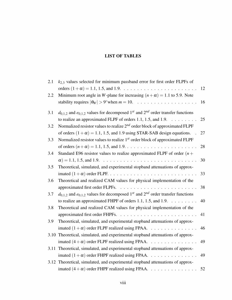
LIST OF TABLES

2.1 k2,3 values selected for minimum passband error for first order FLPFs oforders (1+a) = 1.1, 1.5, and 1.9. . . . . . . . . . . . . . . . . . . . . . . 12

2.2 Minimum root angle in W -plane for increasing (n+a) = 1.1 to 5.9. Notestability requires |qW |> 9�when m = 10. . . . . . . . . . . . . . . . . . . 16

3.1 d0,1,2 and e0,1,2 values for decomposed 1st and 2nd order transfer functionsto realize an approximated FLPF of orders 1.1, 1.5, and 1.9. . . . . . . . . 25

3.2 Normalized resistor values to realize 2nd order block of approximated FLPFof orders (1+a) = 1.1, 1.5, and 1.9 using STAR-SAB design equations. . 27

3.3 Normalized resistor values to realize 1st order block of approximated FLPFof orders (n+a) = 1.1, 1.5, and 1.9. . . . . . . . . . . . . . . . . . . . . . 28

3.4 Standard E96 resistor values to realize approximated FLPF of order (n+a) = 1.1, 1.5, and 1.9. . . . . . . . . . . . . . . . . . . . . . . . . . . . . 30

3.5 Theoretical, simulated, and experimental stopband attenuations of approx-imated (1+a) order FLPF. . . . . . . . . . . . . . . . . . . . . . . . . . . 33

3.6 Theoretical and realized CAM values for physical implementation of theapproximated first order FLPFs. . . . . . . . . . . . . . . . . . . . . . . . 38

3.7 d0,1,2 and e0,1,2 values for decomposed 1st and 2nd order transfer functionsto realize an approximated FHPF of orders 1.1, 1.5, and 1.9. . . . . . . . . 40

3.8 Theoretical and realized CAM values for physical implementation of theapproximated first order FHPFs. . . . . . . . . . . . . . . . . . . . . . . . 41

3.9 Theoretical, simulated, and experimental stopband attenuations of approx-imated (1+a) order FLPF realized using FPAA. . . . . . . . . . . . . . . 46

3.10 Theoretical, simulated, and experimental stopband attenuations of approx-imated (4+a) order FLPF realized using FPAA. . . . . . . . . . . . . . . 49

3.11 Theoretical, simulated, and experimental stopband attenuations of approx-imated (1+a) order FHPF realized using FPAA. . . . . . . . . . . . . . . 49

3.12 Theoretical, simulated, and experimental stopband attenuations of approx-imated (4+a) order FHPF realized using FPAA. . . . . . . . . . . . . . . 52

viii

3.13 Signal power of tones at 3kHz and 10kHz after application to approximatedFHPFs of orders (4+a) = 4.1 to 4.9 in steps of 0.2 . . . . . . . . . . . . 53

4.1 Cumulative error of both magnitude and phase equi-ripple responses com-pared to the original approximation. . . . . . . . . . . . . . . . . . . . . . 62

4.2 Realized CAM values for physical implementation of the 1.8 order FLPFsrealized using the original and equi-ripple approximation, (4.1) and (4.3),respectively. Note b = 3.8382 for the equi-ripple magnitude approximation. 66

4.3 Realized CAM values for physical implementation of the approximatedFLPFs using equi-ripple magnitude approximation. Note b = 3.2907, 3.4199,and 3.8382 for (1+a) = 1.2, 1.5, and 1.8, respectively. . . . . . . . . . . . 66

4.4 Theoretical, simulated, and experimental stopband attenuations of (1+a)

order FLPF approximated with equi-ripple approximation realized usingan FPAA. . . . . . . . . . . . . . . . . . . . . . . . . . . . . . . . . . . . 67

5.1 Component values to realize 2nd order Butterworth LP response with cutofffrequency of 500Hz using the Tow-Thomas Biquad. . . . . . . . . . . . . . 73

5.2 Component values to realize approximated fractional capacitors of 6.5nFand 68nF centered around 500Hz when a = 0.5 using RC ladder topologyof inset in Fig. 5.5. . . . . . . . . . . . . . . . . . . . . . . . . . . . . . . 77

5.3 Component values used to simulate in PSPICE the fractional Tow-Thomasbiquads of Fig. 5.5. . . . . . . . . . . . . . . . . . . . . . . . . . . . . . . 79

5.4 Theoretical, simulated, and experimental stopband attenuations of frac-tional Tow-Thomas biquad realized with the Arbre fractional capacitor. . . 80

ix

LIST OF FIGURES

1.1 Gain characteristic of ideal low pass filter. . . . . . . . . . . . . . . . . . . 21.2 Magnitude response of lowpass Butterworth filter as order increases from

n = 1 to n = 7. . . . . . . . . . . . . . . . . . . . . . . . . . . . . . . . . 3

2.1 Passband peaking in magnitude response of fractional step (1+a) orderfilter for a = 0.1, 0.5, 0.9. . . . . . . . . . . . . . . . . . . . . . . . . . . 9

2.2 Pole angles of (2.2) in the W -plane closest to the region on instability for(n+a) = 1.1, 1.5, 1.9. . . . . . . . . . . . . . . . . . . . . . . . . . . . . 10

2.3 Comparison of FLPF transfer functions of order (n+a) = 1.9. . . . . . . . 112.4 Values of k2,3 to yield minimum passband error compared to the 1st order

butterworth response. . . . . . . . . . . . . . . . . . . . . . . . . . . . . . 132.5 Magnitude response of FLPFs of order (1+a) = 1.1, 1.5, and 1.9 when

k2,3 are selected for minimum passband error. . . . . . . . . . . . . . . . . 132.6 w3dB value for FLPFs of order (1+a) when k2,3 selected for minimum

passband error. . . . . . . . . . . . . . . . . . . . . . . . . . . . . . . . . 142.7 Stability boundaries in the k2 �a plane for the values of k3 = 0.01,0.1,1

and 10. . . . . . . . . . . . . . . . . . . . . . . . . . . . . . . . . . . . . . 152.8 Minimum root angles of FLPF characteristic equations in W -plane com-

pared to stability criteria when m = 100. . . . . . . . . . . . . . . . . . . . 162.9 Magnitude response of higher order FLPF with fractional steps from 5.1 to

5.9. . . . . . . . . . . . . . . . . . . . . . . . . . . . . . . . . . . . . . . 172.10 �3dB frequencies for filters of order (n+a) for n = 2 to 6 using (2.8). . . 182.11 Magnitude response of fractional highpass filters of orders 1.1, 1.5, and 1.9. 192.12 Magnitude response of higher order FHPF with fractional steps from 4.1 to

4.9. . . . . . . . . . . . . . . . . . . . . . . . . . . . . . . . . . . . . . . 20

3.1 Magnitude and phase of s0.5 using 2nd order approximation (dashed) com-pared to ideal case (solid). . . . . . . . . . . . . . . . . . . . . . . . . . . 22

x

3.2 Plot of k2 and k3 versus a that yields minimum passband error in (3.2) andthe interpolated functions as solid and dashed lines, respectively. . . . . . . 23

3.3 Circuit topology of the STAR single-amplifier biquad circuit. . . . . . . . . 253.4 Parallel RC network in the feedback portion of an inverting op-amp to re-

alize a first order transfer function. . . . . . . . . . . . . . . . . . . . . . . 283.5 Circuit topology used in the approximation to the fractional low pass filter

of order (1+a) . . . . . . . . . . . . . . . . . . . . . . . . . . . . . . . . 293.6 (a) Printed circuit board layout and (b) populated board to realize approxi-

mated FLPF of Fig. 3.5. . . . . . . . . . . . . . . . . . . . . . . . . . . . 313.7 (a) Measured and PSPICE simulation results of the magnitude response of

the approximated (1+a) order FLPF, shown as solid and dashed lines,respectively. (b) Step response of approximated 1.9 order FLPF. . . . . . . 32

3.8 Internal switched capacitor circuits on the FPAA to realize the (a) low passbilinear and (b) pole/zero biquadratic transfer functions. . . . . . . . . . . . 35

3.9 First order approximated FLPF implementation using the bilinear and bi-quadratic filter CAMs of the AnadigmDesigner tools for implementationon the AN231E04 FPAA. . . . . . . . . . . . . . . . . . . . . . . . . . . 36

3.10 Parameter setup environment of the AnadigmDesigner tools for the (a) bi-linear and (b) biquadratic filter CAMs. . . . . . . . . . . . . . . . . . . . . 37

3.11 Fourth order approximated FLPF implementation using the bilinear and bi-quadratic filter CAMs of the AnadigmDesigner2 tools for implementationon the AN231E04 FPAA. . . . . . . . . . . . . . . . . . . . . . . . . . . 39

3.12 First order approximated FHPF implementation using the bilinear and bi-quadratic filter CAMs of the AnadigmDesigner2 tools for implementationon the AN231E04 FPAA. . . . . . . . . . . . . . . . . . . . . . . . . . . 41

3.13 Fourth order approximated FHPF implementation using the bilinear and bi-quadratic filter CAMs of the AnadigmDesigner2 tools for implementationon the AN231E04 FPAA. . . . . . . . . . . . . . . . . . . . . . . . . . . 42

3.14 (a) AN231E04 FPAA development kit from Anadigm used to realize frac-tional step filters; (b) test setup to measure the magnitude response of cir-cuits implemented on the AN231E04 with a HP4395A Network analyzer. . 43

3.15 Circuits to realize the (a) level-shifting, single-to-differential and (b) differential-to-single signal conversions to interface the AN231 FPAA with the HP4395Anetwork analyzer. . . . . . . . . . . . . . . . . . . . . . . . . . . . . . . . 45

3.16 Block diagram of test setup with conversion circuits required to interfacethe AN231 FPAA and the HP4395A network analyzer. . . . . . . . . . . . 46

xi

3.17 MATLAB simulation and FPAA experimental results of the (a) magnitudeand (b) phase responses of the approximated (1+a) order FLPF shown assolid and dashed lines, respectively. . . . . . . . . . . . . . . . . . . . . . 47

3.18 MATLAB simulation and FPAA experimental results of the (a) magnitudeand (b) phase responses of the approximated (4+a) order FLPF shown assolid and dashed lines, respectively. . . . . . . . . . . . . . . . . . . . . . 48

3.19 MATLAB simulation and FPAA experimental results of the (a) magnitudeand (b) phase responses of the approximated (1+a) order FHPFs shownas solid and dashed lines, respectively. . . . . . . . . . . . . . . . . . . . . 50

3.20 MATLAB simulation and FPAA experimental results of the (a) magnitudeand (b) phase responses of the approximated (4+a) order FHPFs shownas solid and dashed lines, respectively. . . . . . . . . . . . . . . . . . . . . 51

3.21 Op amp topology with output voltage proportional to the sum of the inputvoltages . . . . . . . . . . . . . . . . . . . . . . . . . . . . . . . . . . . . 52

3.22 Frequency spectrum of approximated 4.5 order FHPF (dashed) comparedto 4th (dotted) and 5th (solid) order highpass Butterworth filters. . . . . . . 54

4.1 Magnitude and phase of ideal (solid) and 2nd order approximation (dashed)of sa when a = 0.7. . . . . . . . . . . . . . . . . . . . . . . . . . . . . . . 56

4.2 Absolute error of inner and outer ripples vs. a of approximated sa com-pared to the ideal of both magnitude and phase responses. . . . . . . . . . . 57

4.3 Minimum b required for stability of (4.3) for 0 < a < 1. . . . . . . . . . . 594.4 Magnitude and phase absolute inner and outer ripple error of (4.3) com-

pared to the ideal sa for b values from 2 to 4 when a = 0.7. . . . . . . . . 604.5 b values required for equi-ripple magnitude (solid) and phase (dashed) er-

ror approximation for 0 < a < 1. . . . . . . . . . . . . . . . . . . . . . . . 614.6 equi-ripple magnitude and phase responses for the cases when a = 0.2 and

a = 0.8. . . . . . . . . . . . . . . . . . . . . . . . . . . . . . . . . . . . . 624.7 FLPF implementation using the bilinear filter, biquadratic filter, and invert-

ing gain CAMs of the AnadigmDesigner2 tools. . . . . . . . . . . . . . . . 644.8 Ideal and approximated magnitude responses of (1+a) = 1.8 order FLPFs

using (4.1) and (4.3) as solid, dashed, and dotted lines, respectively. Notethat for all FLPFs k2 = 1.11 and k3 = 0.966 with b = 3.8382 in (4.3). (b)Step response of approximated 1.8 order FLPF using (4.3). . . . . . . . . . 65

xii

4.9 Measured and MATLAB simulation results of the magnitude response ofthe approximated (1+a) order FLPF, shown as dashed and solid lines,respectively. . . . . . . . . . . . . . . . . . . . . . . . . . . . . . . . . . . 67

5.1 (a) Packaged fractional capacitors implemented using photolithographicfractal structures on silicon, based on the (b) Hilbert and (c) Tree fractalstructures. . . . . . . . . . . . . . . . . . . . . . . . . . . . . . . . . . . . 70

5.2 Tow-Thomas biquad topology. . . . . . . . . . . . . . . . . . . . . . . . . 715.3 Magnitude response of Tow-Thomas and fractional Tow-Thomas biquad

low pass function when a = 0.5 as solid and dashed lines, respectively. . . 745.4 (a) Updated impedance model of Hilbert fractional capacitor and (b) up-

dated Tow-Thomas biquad circuit using updated impedance model. . . . . . 765.5 Fractional Tow-Thomas biquad with approximated fractional capacitors re-

alized with RC ladders for PSPICE simulation of circuits with the (a) Arbreand (b) Hilbert FCs. . . . . . . . . . . . . . . . . . . . . . . . . . . . . . . 78

5.6 Measured (dashed) and PSPICE simulated (solid) results of magnitude re-sponses of fractional Tow-Thomas biquad using Hilbert and Arbre frac-tional capacitors. . . . . . . . . . . . . . . . . . . . . . . . . . . . . . . . 79

A.1 MATLAB simulation and FPAA experimental results of the (a) magnitudeand (b) phase responses of the approximated (1+a) order FLPFs shownas solid and dashed lines, respectively. . . . . . . . . . . . . . . . . . . . . 92




A.5 MATLAB simulation and FPAA experimental results of the (a) magnitudeand (b) phase responses of the approximated (1+a) order FHPFs shownas solid and dashed lines, respectively. . . . . . . . . . . . . . . . . . . . . 96


xiii



B.1 Magnitude response of the approximated fractional capacitor (dashed) com-pared to the ideal fractional capacitor of impedance Z(s) = 1/s0.5. . . . . . 101

B.2 RC ladder network to realize 4th order approximated fractional Laplacianoperator. . . . . . . . . . . . . . . . . . . . . . . . . . . . . . . . . . . . . 101

B.3 Magnitude response of the approximated fractional capacitor (dashed) com-pared to the ideal fractional capacitor of impedance Z(s) = 1/Cs0.5 afterapplying the scalings when C = 6.8nF and wc = 1000rad/s. . . . . . . . . 103

B.4 MAPLE code to calculate resistor and capacitor values for the ladder re-alization of a fractional capacitor, Z(s) = 1/Cs0.5, of 6.8nF at a centrefrequency of 500Hz. . . . . . . . . . . . . . . . . . . . . . . . . . . . . . 104

xiv

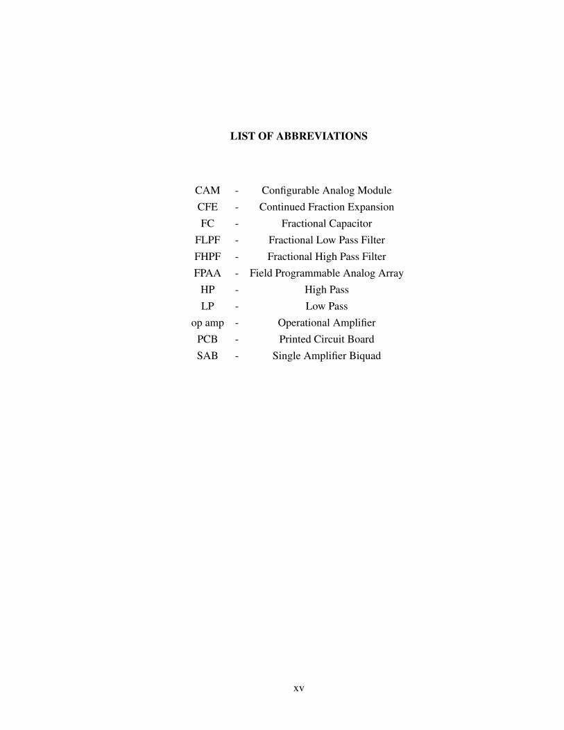
LIST OF ABBREVIATIONS

CAM - Configurable Analog ModuleCFE - Continued Fraction ExpansionFC - Fractional Capacitor

FLPF - Fractional Low Pass FilterFHPF - Fractional High Pass FilterFPAA - Field Programmable Analog Array

HP - High PassLP - Low Pass

op amp - Operational AmplifierPCB - Printed Circuit BoardSAB - Single Amplifier Biquad

xv

CHAPTER 1

INTRODUCTION

1.1 Traditional Filters

Traditional continuous time filters are electronic circuits used in signal processing to di-

rect, channel, integrate, separate, delay, differentiate, attenuate, and transform all kinds of

electric energy and signals [1]. These filters, whether active or passive, can be grouped into

five basic classes based on the shape of the response in the frequency domain. These five

types in their ideal form include:

1. Low Pass: which passes signals from DC to a selected cutoff frequency, and does not

pass all frequencies above that cutoff frequency.

2. High Pass: which allows all signals above a selected cutoff frequency to pass through,

and does not allow all frequencies below through.

3. Band Pass: allows all signals within a selected bandwidth around a selected fre-

quency to pass, but does not allow all frequencies outside of this range.

4. Band Reject: this allows all signals to pass except a selected bandwidth around a

selected frequency.

5. All-Pass: allows all signals to pass but introduces a predictable phase change for

selected frequencies.

Here for all these types the range of frequencies that are passed are referred to as the pass-

band and the range of frequencies not passed are referred to as the stopband. Note the

2

0

0.2

0.4

0.6

0.8

1

1.2

1.4

Frequency (rad/s)

Gai

n

Figure 1.1: Gain characteristic of ideal low pass filter.

ideal filter response of these types would provide no attenuation to all frequencies in the

passband while applying infinite attenuation to all those in the stopband. This ideal low

pass filter is presented in Fig. 1.1, which would transmit all frequencies below the cut-

off frequency, wc, with a gain of 1 and eliminate all frequencies above it with a gain of

0. However, this proves impossible to physically realize and in practice approximations

of the ideal response are instead implemented. The four main approximations, each with

their own distinct advantages and disadvantages, used in implementing electronic filters

are the Butterworth, Chebyshev, Inverse Chebyshev, and Elliptic functions [2]; providing

a maximally flat passband, equal ripple passband, equal ripple stopband, or equal ripple

passband and stopband, respectively. Each of these functions becomes a closer approxi-

mation of the ideal case as the order, n, of the filter increases, where n is an integer value.

These changes in the lowpass Butterworth magnitude characteristics as the order increases

from n = 1 to n = 7 are shown in Fig. 1.2. The transfer functions that describe the circuits

to realize these responses take the form T (s) = N(s)/D(s) where both N(s) and D(s) are

polynomials described using the Laplacian operator, s, raised to an integer order; i.e. s,

s2, . . .sn. Where the order of the filter, n, is chosen to meet the required attenuation of the

3

10−1

100

101

−150

−100

−50

0

Frequency (rad/s)

Mag

nit

ud

e (d

B)

Figure 1.2: Magnitude response of lowpass Butterworth filter as order increases fromn = 1 to n = 7.

filter design specifications.

1.1.1 Selection of Order Based on Design Specifications

When designing traditional filters, the order is determined from the attenuation specifica-

tions that the filter needs to meet. These specifications outline the maximum deviation in

the passband and stopband, Kp and Ks, respectively; and the passband and stopband fre-

quencies at which they occur, wp and ws , respectively. From these requirements the design

equations to determine the order using the Butterworth approximation are [2]

W =ws

wp(1.1)

M =

s100.1Ks �1100.1Kp �1

(1.2)

nB =ln(M)

ln(W)(1.3)

where nB is the order of the Butterworth filter to meet the design requirements. The value

of nB from (1.3) is rarely an integer, which is required for the implementation of the filter,

so in practice it is rounded up to the next integer value. It is this requirement that results

4

in the integer order stepping in the magnitude characteristics of Fig. 1.2. However, by

importing concepts of fractional calculus, we are able to design filters with more precise

control over the stopband characteristics.

1.2 Fractional Calculus

Fractional calculus, the branch of mathematics concerning differentiation and integration

to noninteger orders, is not a new field. With Leibniz writing as early as 1695 about a

12 derivative,

⇣d

12 x⌘

, he commented quite prophetically “from which one day useful con-

sequences will be drawn”. However, the first major study of fractional calculus was not

laid out until 1832 by Liouville in “Memoire sur quelques Questions de Geometrie et de

Mecanique, et sur un noveau genre de Calcul pour resoudre ces Questions” [3].

Where traditional differentiation takes the form dn

dtn f (t), where n is an integer; using

fractional calculus the value of n can be non-integer order, such as 1.3,p

2, 4 � 3i or

any other real or imaginary order. The Riemann-Liouville definition [3–5] of a fractional

derivative, where n�1 < a < n is defined as

da

dta f (t)⌘ Da f (t) =da

dta

2

4 1G(n�a)

tZ

0

f (t)(t � t)a�n+1 dt

3

5 (1.4)

and the definition of a fractional integral where 0 < a < 1 is given as

D�a f (t) =1

G(a)

Z t

0

f (t)(t � t)1�a dt (1.5)

where G(·) is the gamma function. Another interpretation of the fractional derivative is

given by the Grünwald-Letnikov approximation as

Da f (t), limDT!0

(DT )�a

G(�a)

•

Âj=0

G( j�a)

G( j+1)f (t � jDT ) (1.6)

where DT is the integration step. While there are no physical analogies to these derivatives,

5

like slope or area under the curve, they still have many useful applications in diverse fields

of engineering. These include materials theory, diffusion theory, bioengineering, circuit

theory and design [6], control theory [7,8], electromagnetics [9], and robotics [10,11]. The

import of these concepts into circuit theory is relatively new, and has shown applications

in transmission media [3], power electronics [12], integrator [13, 14] and differentiator

circuits [15], oscillators [16], multivibrator circuits [17], and filter theory [18–21] with

potentially many other applications.

1.2.1 Fractional Laplacian Operator

The Laplace transform is a very useful tool in the design and analysis of electronic circuits,

transforming the circuit from the time domain to the frequency domain. This is especially

useful because it allows for the analysis of circuits using algebraic rather than differential

equations [22]. This transformation when applied to a time domain function, f (t), is given

by

L{ f (t)}= F(s) =Z •

0�f (t)e�stdt

where F(s) is the transformed function in the frequency domain, and s is the Laplacian

operator. By applying this transformation to the standard circuit elements of a capacitor

and inductor, with zero initial conditions, we obtain their impedance characteristics in the

frequency domain described as

ZC(s) =1

sCZL(s) = sL

where ZC,L are the impedance of the capacitor and inductor, respectively, in the frequency

domain. While the Laplacian operator in electronic filters has traditionally been raised

to an integer order, it is mathematically valid to raise to a non-integer order, sa , where

0 < a < 1, effectively representing a fractional-order system. Hence, after applying the

6

Laplace transform, with zero initial conditions, to the fractional derivative (1.4) yields

L{0dat f (t)}= saF(s) (1.7)

where sa is the fractional Laplacian operator. The use of the fractional Laplacian opera-

tor allows for the design and analysis of systems using concepts from fractional calculus

without having to solve the difficult time domain representations.

1.3 Research Objectives

While the area of electronic filters is one of the few areas of electrical engineering with a

well defined design procedure; the import of concepts from fractional calculus allows for

the creation of a more general design procedure. With the potential for filters to be designed

to meet the exact design requirements of attenuation, phase, or delay specifications. This

idea of generalizing filter design is a very new field [18,19,21], with much work that needs

to be accomplished in order to create a more generalized filter design procedure.

This research is dedicated to the exploration and importing of concepts from fractional

calculus into continuous time filter design. We accomplish this by exploring previously

proposed fractional step filters which exhibit undesired passband peaking. This leads to the

development of a new fractional step filter, that removes this passband peaking from the

magnitude response of previous filters. Focus has been placed on the design of a fractional

step filter and its physical realization using approximations of the fractional Laplacian op-

erator. The use of fabricated integrated circuit fractional capacitors in the realization of a

biquadratic filter is also explored to realize fractional step filters.

1.4 Thesis Overview

This thesis is divided into three basic areas of research focus. First, the design and imple-

mentation of fractional step filters without the passband peaking of previously proposed

7

filters is presented. Second, a modification of the approximated fractional Laplacian opera-

tor to yield a lower error approximation for use in the physical implementation of fractional

step filters is presented. Finally, the use of fractional capacitors in electronic circuits to ver-

ify the operation of fractional filters is examined.

Chapter 2 begins with a brief introduction to previously designed fractional step filters.

A proposed low pass filter is presented to solve the passband peaking problem experienced

in previous filters. MATLAB simulations of this filter are presented showing the precise

control of the stopband characteristics of a fractional step filter. A method for the imple-

mentation of higher order low pass fractional step filters is also presented with MATLAB

simulations. Last, the application of the low pass to high pass transformation is shown,

again with MATLAB simulations.

Presented in Chapter 3 is the physical realization of these fractional step filters. The de-

sign of these filters using an approximation of the fractional Laplacian operator is outlined,

with physical realizations using operational amplifiers and field programmable analog ar-

rays. Experimental results of these realizations compared to the simulations verify the

operation of these filters.

Chapter 4 presents a modification to a second order approximation of the fractional

Laplacian operator that has lower peak and cumulative error than the original approxi-

mation. This approximation is used in the implementation of fractional step filters with

simulations and experimental results verify its operation.

Presented in Chapter 5 is the use of a fractional capacitor in a Tow-Thomas Biquad

circuit to implement a fractional low pass filter. Theoretical, simulation, and experimental

results presented to verify the operation of a fractional capacitor in an electronic circuit.

Chapter 6 concludes the thesis and suggests improvements for future work.

CHAPTER 2

DESIGN OF FRACTIONAL FILTERS

2.1 Analysis of Previous Fractional Low Pass Filter (FLPF)

The fractional Laplacian operator is especially useful in the design of filters with frac-

tional step characteristics in the stopband; as the design of transfer functions can be done

algebraically rather than through solving the difficult time domain representations of the

fractional derivatives. The transfer function of such a low pass filter is [18]

T (s) =k1

sn+a + k2(2.1)

where n is an integer, k1,2 are positive constants, and 0 < a < 1. The roots of this fractional

equation are s1,2 = k1/(n+a)2 e± j(p/(n+a)) when 1 < n+a < 2. However, when (n+a)< 1

there are no poles in the physical s-plane [18]. Now while this transfer function does pro-

duce a low-pass filter with fractional step of �20(n+a)dB/dec through the stopband,

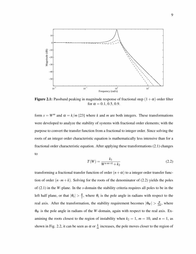
it also has the undesired quality of having a peak in the passband. This peaking is il-

lustrated for (n+a) = 1.1, 1.5, 1.9 when k1 = k2 = 1 as shown in Fig. 2.1. With the

maximum peak for each case reaching a value of k1/hk2sin (n+a)p

2

i, resulting in peaks at

0.1076, 3.01, 16.11dB for (n+a) = 1.1, 1.5, 1.9, respectively.

2.1.0.1 Roots of the W -plane

To further investigate the cause of the peaking in the magnitude response of (2.1) requires

the transformation from the s-domain to the W -domain through application of the trans-

9

10−2

10−1

100

101

−50

−40

−30

−20

−10

0

10

Frequency (rad/s)

Mag

nit

ud

e (d

B)

Figure 2.1: Passband peaking in magnitude response of fractional step (1+a) order filterfor a = 0.1, 0.5, 0.9.

form s = W m and a = k/m [23] where k and m are both integers. These transformations

were developed to analyze the stability of systems with fractional order elements; with the

purpose to convert the transfer function from a fractional to integer order. Since solving the

roots of an integer order characteristic equation is mathematically less intensive than for a

fractional order characteristic equation. After applying these transformations (2.1) changes

to

T (W ) =k1

W n·m+k + k2(2.2)

transforming a fractional transfer function of order (n+a) to a integer order transfer func-

tion of order (n ·m+ k). Solving for the roots of the denominator of (2.2) yields the poles

of (2.1) in the W -plane. In the s-domain the stability criteria requires all poles to be in the

left half plane, or that |qs| > p2 , where qs is the pole angle in radians with respect to the

real axis. After the transformation, the stability requirement becomes |qW | > p2m , where

qW is the pole angle in radians of the W -domain, again with respect to the real axis. Ex-

amining the roots closest to the region of instability when k2 = 1, m = 10, and n = 1, as

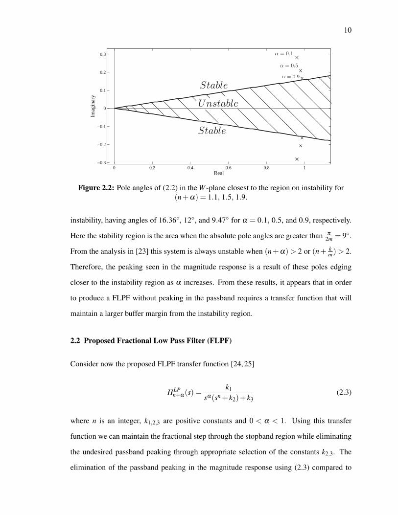
shown in Fig. 2.2, it can be seen as a or km increases, the pole moves closer to the region of

10

0 0.2 0.4 0.6 0.8 1−0.3

−0.2

−0.1

0

0.1

0.2

0.3

Real

Imag

inar

y

Figure 2.2: Pole angles of (2.2) in the W -plane closest to the region on instability for(n+a) = 1.1, 1.5, 1.9.

instability, having angles of 16.36�, 12�, and 9.47� for a = 0.1, 0.5, and 0.9, respectively.

Here the stability region is the area when the absolute pole angles are greater than p2m = 9�.

From the analysis in [23] this system is always unstable when (n+a)> 2 or (n+ km)> 2.

Therefore, the peaking seen in the magnitude response is a result of these poles edging

closer to the instability region as a increases. From these results, it appears that in order

to produce a FLPF without peaking in the passband requires a transfer function that will

maintain a larger buffer margin from the instability region.

2.2 Proposed Fractional Low Pass Filter (FLPF)

Consider now the proposed FLPF transfer function [24, 25]

HLPn+a(s) =

k1

sa(sn + k2)+ k3(2.3)

where n is an integer, k1,2,3 are positive constants and 0 < a < 1. Using this transfer

function we can maintain the fractional step through the stopband region while eliminating

the undesired passband peaking through appropriate selection of the constants k2,3. The

elimination of the passband peaking in the magnitude response using (2.3) compared to

11

10−2

10−1

100

101

102

−80

−70

−60

−50

−40

−30

−20

−10

0

10

20

Frequency (rad/s)

Mag

nit

ude

(dB

)

Figure 2.3: Comparison of FLPF transfer functions of order (n+a) = 1.9.

(2.1) is shown in Fig. 2.3 for the case when 1+a = 1.9 and constants k2 = 1.31 and

k3 = 0.99. Notice that the passband of (2.3) remains flat while (2.1) has a peak of 16.11dB.

2.2.1 Selection of k2,3 for Flat Passband Response

By modifying k2,3 in (2.3) the passband of the magnitude response can be shaped without

altering the stopband region. Therefore, through their careful selection the passband region

can be shaped to better resemble the passband of a Butterworth response while maintaining

the desired fractional step. That is, the selection of the constants k2,3 when k1 = 1 for

minimum passband error can be done numerically; with the cumulative magnitude error

compared to the Butterworth response through the passband calculated up until the �3dB

frequency w0. The combination of k2 and k3 that yield the lowest cumulative error selected

for each a . This cumulative magnitude error, |EC( jw)|, is calculated as

|EC( jw)|=N

Âi=1

�� |B1( jwi)|��HLP

1+a( jwi)�� (2.4)

12

Order (1+a) k2 k3

1.1 0.245 0.831.5 0.594 0.9121.9 1.315 0.986

Table 2.1: k2,3 values selected for minimum passband error for first order FLPFs of orders(1+a) = 1.1, 1.5, and 1.9.

where |B1( jwi)| is the magnitude response at frequency wi of the first order low-pass But-

terworth filter,��HLP

1+a( jwi)�� is the magnitude response of the FLPF of order (1+a) at

frequency wi, and N is the number of samples. For our analysis N = 200 where the range

of frequencies is w e [0.01,1]. For each value of a between 0.01 and 0.99 in steps of 0.01,

the cumulative error was calculated for all combinations of 0 < k2 < 2 and 0 < k3 < 1 in

steps of 0.001. From all the cumulative errors collected for each a , the combination that

resulted in the minimum error was selected. These values that yield the minimum passband

error as well the interpolated functions to match the collected data are shown in Fig. 2.4 as

solid and dashed lines, respectively. The interpolated quadratic and linear functions from

the collected raw data for k2,3, respectively, are

k2 = 1.1796a2 +0.16765a +0.21735 (2.5)

k3 = 0.19295a +0.81369 (2.6)

with a norm of residuals, R, of 0.090685 and 0.024265 for the interpolated functions of k2

and k3, respectively. This norm of residuals is calculated from the fit residuals, defined as

the difference between the ordinate data point and the resulting fit for each abscissa data

point; with a lower norm value indicating a better fit than a larger value.

The magnitude response of FLPFs of order (1+a) = 1.1, 1.5, and 1.9 when the values

of k2,3 for minimum passband error are used are shown in Fig. 2.5. The values of k2,3

selected for minimum passband error for these filters are given in Table 2.1. Note that

these values do not produce a true fractional Butterworth response as the DC gain, k1/k3,

13

0 0.1 0.2 0.3 0.4 0.5 0.6 0.7 0.8 0.9 10

0.2

0.4

0.6

0.8

1

1.2

1.4

1.6

Figure 2.4: Values of k2,3 to yield minimum passband error compared to the 1st orderbutterworth response.

10−2

10−1

100

101

102

−90

−80

−70

−60

−50

−40

−30

−20

−10

0

10

Frequency (rad/s)

Mag

nit

ude

(dB

)

Figure 2.5: Magnitude response of FLPFs of order (1+a) = 1.1, 1.5, and 1.9 when k2,3are selected for minimum passband error.

is not unity and a �3dB frequency of 1rad/s is not maintained. It instead provides a flat

passband response with the minimum error when compared to the 1st order Butterworth

over the frequency range 0.01rad/s to 1rad/s. It is still possible to set the DC gain of

these filters to unity by setting k1 = k3, which still maintains the flat passband of the filter.

14

0 0.1 0.2 0.3 0.4 0.5 0.6 0.7 0.8 0.9 1

0.9

0.95

1

1.05

1.1

1.15

Figure 2.6: w3dB value for FLPFs of order (1+a) when k2,3 selected for minimumpassband error.

In addition, the �3dB frequency, w3dB, of (2.3) is nonlinearly dependent on the values of

k2,3 and a . The numerical solution of w3dB, for 0 < a < 1 in steps of 0.01 for FLPFs of

order (1+a) when k2,3 are selected for minimum passband error are shown in Fig. 2.6.

Note that the maximum and minimum deviations occur at a = 0.45 and 0.99 with �3dB

frequencies of 1.1602rad/s and 0.8917rad/s, respectively. In the section that follows we

examine the stability analysis of the proposed equation (2.3).

2.2.2 Stability Analysis

To analyze the stability of the proposed FLPF we transform the transfer function from the

s-plane to the W -plane, again using the transformations s = W m and a = k/m [23]. After

applying this transformation, (2.3) changes to,

T (W ) =k1

W n·m+k + k2W k + k3(2.7)

whose characteristic equation in the W -plane must be solved to ensure that it meets the

stability criteria. Setting the denominator of (2.7) to zero and solving for W yields (n ·m+k)

15

-10

-8

-6

-4

-2

0

0 0.2 0.4 0.6 0.8 1

Figure 2.7: Stability boundaries in the k2 �a plane for the values of k3 = 0.01,0.1,1 and10.

roots. Stability requires that | qW |> p2m for all poles of the characteristic equation, where

qW is the pole angle in radians. If any of the pole angles do not meet this criteria then the

system is unstable. Through numerical analysis of this characteristic equation it was found

that the system is always unstable when n+ (k/m) > 2 regardless of the values of k2,3.

While for the region n+(k/m)< 2 there are always values of k2,3 that will ensure stability

of the system. An example of the stability boundary in the k2 �a plane to four values of

k3 are shown in Fig. 2.7 for the case of m = 100 and n = 1.

2.2.2.1 Minimum Root Angle in W -plane

Where previously the roots of the (2.2) were shown to move very close to the region of

instability as a approaches the stability limit, the roots of (2.7) maintain a much larger

margin from the unstable region. The differences between the minimum angle of the roots

for the characteristic equations (2.2) and (2.7), when n = 1 and the k2,3 values are selected

for minimum passband error, are shown in Fig. 2.8. Where the solid line is the minimum

16

0 0.1 0.2 0.3 0.4 0.5 0.6 0.7 0.8 0.9 10.8

0.9

1

1.1

1.2

1.3

1.4

1.5

1.6

1.7

1.8

k/m

An

gle

(d

egre

es)

Figure 2.8: Minimum root angles of FLPF characteristic equations in W -plane comparedto stability criteria when m = 100.

Minimum Root Angle (�)n a = 0.1 a = 0.3 a = 0.5 a = 0.7 a = 0.91 16.71 14.89 13.86 13.50 13.752 8.67 8.15 7.84 7.72 7.773 5.85 5.61 5.46 5.39 5.404 4.41 4.28 4.19 4.15 4.145 3.55 3.46 3.40 3.37 3.36

Table 2.2: Minimum root angle in W -plane for increasing (n+a) = 1.1 to 5.9. Notestability requires |qW |> 9�when m = 10.

angle required for stability when m = 100, with all values above lying in the stable region

and all those below in the unstable region. Note that as k/m increases the minimum root

angle of (2.2) moves closer to the instability region, whereas the minimum root angle of

(2.7) maintains a much larger margin of stability. Using the values for minimum passband

error, as the order n of the filter increases the minimum root angle of (2.7) is within the

unstable region regardless of the value of a . A sample of these minimum angles are given

in Table 2.2. All of the values for n > 1 are within the unstable region, being less than the

angle required for stability, |qW | < p2m = 9�. Hence, to maintain stability the order of the

filter must be limited to an order of (n+a) < 2 because increasing n above 1 moves the

minimum root angle of the characteristic equation into the unstable region of the W -plane.

17

10−1

100

101

102

−250

−200

−150

−100

−50

0

Frequency (rad/s)

Mag

nit

ude

(dB

)

Figure 2.9: Magnitude response of higher order FLPF with fractional steps from 5.1 to5.9.

2.2.3 Implementation of Higher Order Fractional Low Pass Filters (FLPF)

While the highest order that (2.3) can implement while maintaining stability without the

undesired passband peaking is n+a < 2, one method of implementing higher order filters

with fractional step is to employ HLP1+a(s), which always has a stable region based on k2,3

when 0 < a < 1 , divided by a higher-order normalized Butterworth polynomial [26]. This

creates a stable higher order fractional step filter of order n+a which can be written as,

HLPn+a(s) =

HLP1+a(s)

Bn�1(s); n � 2 (2.8)

where Bn(s) is a standard Butterworth polynomial of order n. Using this method we can cre-

ate stable higher order filters with a fractional step through the stopband while maintaining

the flat passband response. Figure 2.9 displays the magnitude response of the fractional-

step lowpass filter of order (5+a) for values of a =0.1, 0.5, 0.9. Note that the values of

k2,3 used in the higher order filter to minimize the passband error are the same as those cal-

culated for filters of order (1+a) presented in Fig. 2.4. While this method of implementing

18

0 0.1 0.2 0.3 0.4 0.5 0.6 0.7 0.8 0.9 1

0.65

0.7

0.75

0.8

0.85

0.9

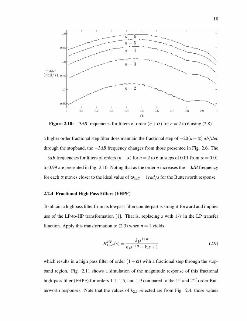
Figure 2.10: �3dB frequencies for filters of order (n+a) for n = 2 to 6 using (2.8).

a higher order fractional step filter does maintain the fractional step of �20(n+a) db/dec

through the stopband, the �3dB frequency changes from those presented in Fig. 2.6. The

�3dB frequencies for filters of orders (n+a) for n = 2 to 6 in steps of 0.01 from a = 0.01

to 0.99 are presented in Fig. 2.10. Noting that as the order n increases the �3dB frequency

for each a moves closer to the ideal value of w3dB = 1rad/s for the Butterworth response.

2.2.4 Fractional High Pass Filters (FHPF)

To obtain a highpass filter from its lowpass filter counterpart is straight-forward and implies

use of the LP-to-HP transformation [1]. That is, replacing s with 1/s in the LP transfer

function. Apply this transformation to (2.3) when n = 1 yields

HHP1+a(s) =

k1s1+a

k3s1+a + k2s+1(2.9)

which results in a high pass filter of order (1+a) with a fractional step through the stop-

band region. Fig. 2.11 shows a simulation of the magnitude response of this fractional

high-pass filter (FHPF) for orders 1.1, 1.5, and 1.9 compared to the 1st and 2nd order But-

terworth responses. Note that the values of k2,3 selected are from Fig. 2.4, those values

19

10−2

10−1

100

101

102

−80

−70

−60

−50

−40

−30

−20

−10

0

Mag

nit

ude

(dB

)

Frequency (rad/s)

Figure 2.11: Magnitude response of fractional highpass filters of orders 1.1, 1.5, and 1.9.

for minimum passband error for the FLPFs. Using these values maintains the flat passband

response after application of the lowpass to highpass transformation.

2.2.4.1 Higher Order Fractional High Pass Filter

Higher order FHPFs are obtained using the same method described for the FLPF. Where the

low-pass filter was divided by a normalized Butterworth polynomial, the high-pass filter is

divided by the normalized Butterworth polynomial after applying the lowpass-to-highpass

transformation. This creates a higher order high-pass fractional filter of order n+a that

can be written as

HHPn+a(s) =

HHP1+a(s)

BHPn�1(s)

; n � 2 (2.10)

where BHPn (s) is a standard Butterworth polynomial of order n after applying the LP to HP

transformation. Fig. 2.12 displays the magnitude response of the fractional-step highpass

filter of order (4+a) for values of a = 0.1, 0.5, 0.9. Note that the values of k2,3 for flat

passband response in the higher order filters of Fig. 2.12 are again the same as those for

the lowpass filters of order (1+a), presented in Fig. 2.4.

20

10−2

10−1

100

101

102

−200

−180

−160

−140

−120

−100

−80

−60

−40

−20

0

Frequency (rad/s)

Mag

nit

ud

e (d

B)

Figure 2.12: Magnitude response of higher order FHPF with fractional steps from 4.1 to4.9.

2.3 Summary

This chapter first examined the cause of the passband peaking in previously proposed frac-

tional low pass filters [18]. An understanding of the problem led to the proposal of a new

fractional low pass transfer function that maintains the fractional step through the stopband

while maintaining a flat passband. The stability of this fractional step filter was investi-

gated, showing it is always stable for orders (n+a) < 2. To realize fractional step filter

of orders (n+a) > 2 a method using the first order FLPF divided by a Butterworth poly-

nomial of order (n� 1) to implement the desired order was proposed. The application

of the lowpass to highpass transformation was presented to create a fractional high pass

filter, with the same method presented to create higher order high pass fractional step fil-

ters. MATLAB simulations were presented to confirm the low and high pass fractional step

filters and the method to implement them in orders greater than (n+a)> 2.

CHAPTER 3

PHYSICAL REALIZATION OF FRACTIONAL FILTERS

3.1 Approximation of the Fractional Laplacian Operator

The use of the fractional Laplacian operator, sa , has theoretically been shown to produce

filters with a fractional step through the stopband [18, 19, 21]. However, there are no com-

mercial fractance devices available for the physical realization of these filters. While most

capacitors do exhibit fractional behaviour [27, 28] and should be modeled with impedance

ZC = 1saC , the value of a is very near to 1 preventing their use in implementing fractional

filters with complete control of the stopband attenuations. Therefore, until commercial

fractance devices become available to physically realize circuits that make use of the ad-

vantages of sa , integer order approximations have to be used. There are many methods

used to create an approximation of sa that include Continued Fraction Expansions (CFEs)

as well as rational approximation methods [7, 29–32]. These methods present a large array

of approximations with varying order and accuracy, with the accuracy and approximated

frequency band increasing as the order of the approximation increases. Using the CFE

method of [32] we obtain the following approximation for the general Laplacian operator

to 2nd order as

sa u (a2 +3a +2)s2 +(8�2a2)s+(a2 �3a +2)(a2 �3a +2)s2 +(8�2a2)s+(a2 +3a +2)

(3.1)

Note that when a = 0.5, (3.1) reverts back to the approximation of s0.5 in [32]. Figure

3.1 shows an example of the magnitude and phase of the approximation of the fractional

22

10−2

10−1

100

101

102

−20

−10

0

10

20

Frequency (rad/s)

Mag

nit

ude

(dB

)

Ideal

2nd Order Approximation

10−2

10−1

100

101

102

0

20

40

60

Frequency (rad/s)

Phas

e (d

egre

es)

Figure 3.1: Magnitude and phase of s0.5 using 2nd order approximation (dashed)compared to ideal case (solid).

Laplacian operator for the case when a = 0.5 compared to the ideal case. For this case it

can be observed that for w 2 [0.032,31.53] the magnitude error does not exceed 1.375dB

while for w 2 [0.142,7.00] the phase error does not exceed 3.2�. Using a second order

approximation for the Laplacian operator results in an (n+2) integer order filter to approx-

imate the (n+a) fractional step filter. This is less expensive to implement in hardware

over approximations of higher order [7, 33]. While (3.1) forms the basis of this chapter,

in Chapter 4 we present a means of creating an equal ripple approximation of the second

order approximated fractional Laplacian operator.

Using (3.1) it can be shown that the transfer function for the FLPF between 1st and 2nd

order changes to,

HLP1+a =

k1

sa(s+ k2)+ k3

u k1

a0

(a2s2 +a1s+a0)

s3 + c0s2 + c1s+ c2(3.2)

where a0 = a2 + 3a + 2, a1 = 8� 2a2, a2 = a2 � 3a + 2, c0 = (a1 + a0k2 + a2k3)/a0,

23

0 0.1 0.2 0.3 0.4 0.5 0.6 0.7 0.8 0.9 10.2

0.4

0.6

0.8

1

1.2

1.4

1.6

Figure 3.2: Plot of k2 and k3 versus a that yields minimum passband error in (3.2) andthe interpolated functions as solid and dashed lines, respectively.

c1 = (a1(k2 + k3)+ a2)/a0 and c2 = (a0k3 + a2k2)/a0. When using the approximation of

the Laplacian operator, the constants k2,3 that yield the passband closest to the Butterworth

response vary from those used for the ideal transfer function. Using the same process

described in Section 2.2.1, the values that yield the minimum passband error when using

the approximation as well the interpolated functions to match the collected data are shown

in Fig. 3.2 as solid and dashed lines, respectively. The interpolated quadratic and linear

functions from the collected raw data for k2,3, respectively, are

k2 = 1.0683a2 +0.161a +0.3324 (3.3)

k3 = 0.29372a +0.71216 (3.4)

with a norm of residuals, R, of 0.15239 and 0.034421 for the interpolated functions of k2

and k3, respectively. Comparing (2.5) and (2.6) with (3.3) and (3.4), respectively, one can

observe that both k2 and k3 in (2.5) and (2.6) are larger for all a than in (3.3) and (3.4).

This is due to the approximation (3.1) used for sa .

24

3.2 Operational Amplifier Approximated FLPF Implementation

To realize the transfer function of (3.2) we can decompose it into first and second order

transfer functions that can be realized using first order and second order single amplifier bi-

quad (SAB) circuit topologies. For our realization, the two transfer functions we generated

were

H(s) = H1(s) ·H2(s)

=1

s+d0· e0s2 + e1s+ e2

s2 +d1s+d2(3.5)

Coefficients d0,1,2 and e0,1,2 are determined through the solution of the system of equations

by equating like terms of (3.2) and (3.5). The following system of equations yields the

coefficients d0,1,2 and e0,1,2

d0 = RootO f [aox3 � (a1 +a0k2 +a2k3)x2 (3.6)

+(a1k2 +a1k3 +a2)x� (a2k2 +a0k3)]

d1 =a1 +a0k2 +a2k3

a0�d0 (3.7)

d2 =a1k2 +a1k3 +a2

a0�d0d1 (3.8)

e0 = k1a2

a0(3.9)

e1 = k1a1

a0(3.10)

e2 = k1 (3.11)

where x is a dummy variable and d0 is a positive real root of (3.6). The values of d0,1,2

and e0,1,2 using (3.6) to (3.11) and k2,3 from Fig. 3.2 when k1 = 1 for filters of order

(1+a) = 1.1, 1.5, and 1.9 are given in Table 3.1.

25

(n+a) k2k3

d0 d1 d2 e0 e1 e2

(1+0.1)0.350.74 0.3056 4.0467 3.2689 0.7403 3.4545 1.0000

(1+0.5)0.690.86 0.4511 2.4109 2.2125 0.2000 2.0000 1.0000

(1+0.9)1.360.97 0.6920 1.8452 1.4409 0.0120 1.1579 1.0000

Table 3.1: d0,1,2 and e0,1,2 values for decomposed 1st and 2nd order transfer functions torealize an approximated FLPF of orders 1.1, 1.5, and 1.9.

+

-

Figure 3.3: Circuit topology of the STAR single-amplifier biquad circuit.

3.2.1 Realization of the 2nd Order Block H2(s)

The 2nd order block, H2(s), having both poles and zeros can be realized using the STAR-

SAB topology [34] shown in Fig. 3.3.

Given the transfer function, H2(s) = e0s2+e1s+e0s2+d1s+d2 , the component values required to re-

alize it using the STAR-SAB topology can be determined using the following steps [2]

1. Set all capacitors, C, to the value of unity to simplify calculations.

2. Choose a value for the positive-feedback parameter K.

26

3. Choose an impedance normalized value for the resistor Rb. Let Rb = 1W.

4. Determine the values of Rc and Ra from

Rc =Ke0

Ra =K

1� e0

5. To simplify computational steps, two constants x1 and x2 are defined as

x1 =2K

�d1 +q

d21 +8Kd2

x2 =e0 +2e2x2

1 � e1x1

1+K

6. Use the constants x1 and x2 to find the values of R1 and R4 as

R1 =x1

x2

R4 =R1x1

R1 � x1

7. Again, to simplify computations, two additional constants y1 and y2 are defined. The

constant y1 must be selected arbitrarily so that it satisfies 0 y1 1 in order that that

the constant y2 is nonnegative and given by

y2 =(1+K)(e0 � y1)

x1d2(e2/d2 � e0)

8. Use the constants y1 and y2 and other terms to find the values of the resistors R2, R3,

27

(1+a) k2k3

, K, y1

Resistor (W) (1+0.1)0.350.74, 10, 1 (1+0.5)0.69

0.86, 5, 0.1 (1+0.9)1.360.97, 0.1, 0

Ra 38.5000 6.2500 0.1020Rb 1.0000 1.0000 1.0000Rc 13.5088 25.0000 5.0090R1 60.6288 6.7755 4.3630R2 0.0766 0.1064 0.2470R3 1.2700 7.8570 •R4 1.6269 1.7168 0.8204R5 • 0.8730 0.0327

Table 3.2: Normalized resistor values to realize 2nd order block of approximated FLPF oforders (1+a) = 1.1, 1.5, and 1.9 using STAR-SAB design equations.

and R5 as

R2 =y2

x1y2d2 +K

R3 =y2

y1

R5 =R3y2

R3 � y2

Using this design procedure, the resistor values for the cases a = 0.1, 0.5, and 0.9 when

using the values of k2,3 for minimum passband error are calculated and given in Table 3.2.

3.2.2 Realization of the 1st Order Block H1(s)

The 1st order block, H1(s), can be realized using a simple parallel RC network in the

feedback portion of an inverting op-amp as presented in Fig. 3.4. The transfer function of

this topology is given byVo(s)Vin(s)

=� 1R7C

1s+ 1

R6C(3.12)

Using this configuration, the resistor capacitor combination of R6C is used to set the time

constant while R6/R7 is used to set the gain of the circuit. The value of R6 required to

realize the first order block for the approximated FLPF realization can be calculated by

28

+

-

Figure 3.4: Parallel RC network in the feedback portion of an inverting op-amp to realizea first order transfer function.

(1+a) k2k3

Resistor (W) (1+0.1)0.350.74 (1+0.5)0.69

0.86 (1+0.9)1.360.97

R6 3.271 2.216 1.445R7 0.931 0.960 1.060

Table 3.3: Normalized resistor values to realize 1st order block of approximated FLPF oforders (n+a) = 1.1, 1.5, and 1.9.

equating H1(s) from (3.5) with (3.12) yielding:

d0 =1

R6C(3.13)

while the DC gain of this block can be set using:

DC gain =R6

R7(3.14)

Using these design equations, the values of R6 and R7 needed to realize the first order block

of the approximated FLPF for a = 0.1, 0.5, and 0.9 when C = 1F are given in Table 3.3.

29

+

+

-

-

Figure 3.5: Circuit topology used in the approximation to the fractional low pass filter oforder (1+a)

3.2.3 Simulation and Experimental Results

The final circuit topology of the fractional low pass filter of order (1+a) is shown in Fig.

3.5 which is a result of a cascade of the first and second order blocks previously described.

This circuit was simulated using PSPICE for filters of order (1+a) for the cases a =

0.1, 0.5, and 0.9. These simulations were conducted with general purpose MC1458 op

amps (1MHz gain bandwidth product) [35]. All time constants were scaled to 0.1ms using

unit resistors of 1kW and capacitors of 0.1uF . This results in all pole frequencies being

shifted from the normalized value of 1rad/s to 104rad/s. The theoretical resistor values

were rounded to the nearest standard E96 (1%) value and are given in Table 3.4. The flat

passband response of this simulated filter for the case of a = 0.1,0.5 and 0.9 is shown in

Figure 3.7(a) as dashed lines where the slope can be observed to change with a .

3.2.3.1 Printed Circuit Board Realization

To further verify the simulations of the FLPF, a printed circuit board (PCB) of the circuit

of Fig. 3.5 was developed. Both the layout and photo of the populated board are shown in

Fig. 3.6. The components used to implement filters of order 1.1, 1.5, and 1.9 consisted of

30

(1+a) k2k3

Resistor (W) (1+0.1)0.350.74 (1+0.5)0.69

0.86 (1+0.9)1.360.97

Ra 38300 6190 102Rb 1000 1000 1000Rc 13700 24900 4990R1 60400 6810 4320R2 76.8 105 249R3 1270 7870 •R4 1620 1740 825R5 • 866 32.4R6 3240 2210 1430R7 931 960 1060

Table 3.4: Standard E96 resistor values to realize approximated FLPF of order(n+a) = 1.1, 1.5, and 1.9.

1% tolerance resistors, 20% tolerance capacitors, and MC1458 op amps. The magnitude

response of these circuits measured using a HP4395A Network analyzer are also shown

in Fig. 3.7(a), but as solid lines. The experimental results show close agreement with the

simulations confirming the operation of the approximated FLPF. The step response of the

1.9 order filter was also investigated to examine its stability, and is shown in Fig. 3.7(b). We

can clearly see from the magnitude response of both the measured and simulated responses

that this filter does realize a fractional step through the stopband without the undesirable

peaking of previous fractional step filters. This verifies the simulations proving that the

integer order filters can accurately approximate the incremental stepping of FLPFs. Also,

as in the simulation results, the measured stopbands are not as linear as the magnitude

response of the simulated transfer function; which is a result of the deviation from the ideal

Laplacian operator associated with using the 2nd order approximation of (3.1). Comparing

the results, we find that the passband attenuations of the experimental and simulated filters

are very close to their theoretical values of �20(1+a)dB/decade. For comparison, these

attenuations are listed in Table 3.5.

31

(a)

(b)

Figure 3.6: (a) Printed circuit board layout and (b) populated board to realizeapproximated FLPF of Fig. 3.5.

3.3 Field Programmable Analog Array Implementation

A Field Programmable Analog Array (FPAA) is an “analog signal processor” specifically

designed for signal conditioning, filtering, gain, rectification, summing, subtracting, and

32

-60

-50

-40

-30

-20

-10

0

10

103

104

105

Magnit

ude (

dB

)

Frequency (rad/s)

(a)

(b)

Figure 3.7: (a) Measured and PSPICE simulation results of the magnitude response of theapproximated (1+a) order FLPF, shown as solid and dashed lines, respectively. (b) Step

response of approximated 1.9 order FLPF.

33

Order Theoretical Simulated Experimental(1+a) (dB/dec) (dB/dec) (dB/dec)

1.1 �22 �22.48 �22.931.5 �30 �29.20 �29.741.9 �38 �36.50 �36.44

Table 3.5: Theoretical, simulated, and experimental stopband attenuations ofapproximated (1+a) order FLPF.

multiplying of signals [36]. The FPAAs from Anadigm consist of fully Configurable Ana-

log Modules (CAMs) surrounded by programmable interconnect and analog input/output

cells. The signal processing occurs in the CAMs using fully differential switched capacitor

circuitry, which provide specialized behaviours such as filtering, gain, sample and hold,

summing, rectification and more. This provides a very flexible architecture that can be

easily reconfigured using the AnadigmDesigner tools. These tools are a graphical design

environment to build circuits using the design CAMs. In this design environment CAMs

can be dropped in, wired together, and configured for the desired design requirements.

From the graphical implementation of a circuit, the AnadigmDesigner tools generate the

configuration data file to program the FPAA. Two CAMs that are particularly useful in

the implementation of approximated fractional step filters are the bilinear and biquadratic

CAMs. Both these modules allow the lowpass and highpass fractional step filters to be

easily implemented.

3.3.1 FPAA Realization of a (1+a) Fractional Low Pass Filter

Previously, to implement an approximated FLPF required the determination of the set of

component values to realize the decomposed transfer functions. Using the biquadratic and

blinear filter CAMs from the AnadigmDesigner tools instead, requires only the transfer

function pole and zero frequencies and quality factors to be realized [37]. For the FPAA

implementation of a first order FLPF, the transfer function of (3.5) must be arranged to

34

match the CAMs, taking the form

T (s) = T1(s) ·T2(s) (3.15)

T1(s) =2p f1G1

s+2p f1

T2(s) = �G2s2 +

2p f2zQ2z

s+4p2 f 22z

s2 +2p f2pQ2p

s+4p2 f 22p

where T1(s) and T2(s) are the transfer functions of the bilinear and biquadratic filter CAMs,

respectively. Here G1,2 are the gains of T1(s) and T2(s) respectively, f1 the pole frequency

of T1(s), f2p,z the pole and zero frequencies of T2(s), and Q2p,z the pole and zero quality

factors of T 2(s). T1(s) and T2(s) are realized on the FPAA using the switched capacitor

circuits in Fig. 3.8 [38, 39]. Before equating the biquadratic and bilinear transfer functions

of (3.5) to (3.15) the frequency transformation of s = swo

= s2p fo must be applied to (3.5),

where fo is the denormalized frequency yielding,

Hdenorm(s) = Hdenorm1(s) ·Hdenorm2(s) (3.16)

Hdenorm1(s) =2p fo

s+2pd0 fo

Hdenorm2(s) =e0

hs2 + 2p f0e1

e0s+ 4p2 f 2

o e2e0

i

s2 +2p f0d1s+4p2 f 2o d2

Comparing the equations of (3.15) and (3.16) the design equations to implement an ap-

proximated FLPF of order (1+a) are

f1 = d0 fo (3.17)

f2z = fo

re2

e0(3.18)

Q2z =

pe0e2

e1(3.19)

35

(a)

(b)

Figure 3.8: Internal switched capacitor circuits on the FPAA to realize the (a) low passbilinear and (b) pole/zero biquadratic transfer functions.

f2p = fop

d2 (3.20)

Q2p =

pd2

d1(3.21)

G1 =e0

d0(3.22)

36

Figure 3.9: First order approximated FLPF implementation using the bilinear andbiquadratic filter CAMs of the AnadigmDesigner tools for implementation on the

AN231E04 FPAA.

3.3.1.1 First Order Approximated Fractional Low Pass Filter

To implement a first order FLPF using a second order approximation requires the use of

both the bilinear and biquadratic filter CAMs. These two CAMs are cascaded and wired

together to the desired input and output ports in the AnadigmDesigner design environment

as shown in Fig. 3.9. The bilinear filter is setup in the low-pass configuration, shown in Fig.

3.10(a), and the biquadratic filter is setup in the pole-zero configuration, as shown in Fig.

3.10(b). Using these setup environments in the AnadigmDesigner tools gives control over

filter type, sampling phase, polarity, resource usage, and design parameters. With the de-

sign parameters giving full control over the corner frequencies, quality factors, and low and

high frequency gains. These tools allow for the design using high level parameters without

the need to calculate the underlying capacitor values to realize the filter with the switched

capacitor circuit. For these approximated FLPFs, the theoretical design values using (3.17)

to (3.22) when f0 = 1kHz and the physical values realized using the CAMs are given in

Table 3.6 for filters of order (1+a) = 1.1, 1.5, and 1.9. Note that the realized values vary

37

(a)

(b)

Figure 3.10: Parameter setup environment of the AnadigmDesigner tools for the (a)bilinear and (b) biquadratic filter CAMs.

38

Order (1+a)1.1 1.5 1.9

Design Value Theoretical Realized Theoretical Realized Theoretical Realizedf1(kHz) 0.305 0.309 0.455 0.456 0.697 0.699f2p(kHz) 1.81 1.81 1.48 1.47 1.20 1.21f2z(kHz) 1.16 1.17 2.24 2.23 7.08 7.15

Q2p 0.447 0.445 0.618 0.619 0.653 0.637Q2z 0.249 0.249 0.224 0.225 0.122 0.122G1 2.42 2.40 0.443 0.429 1.00 1.00A 1.00 1.00 1.00 1.00 0.0173 0.0287

Table 3.6: Theoretical and realized CAM values for physical implementation of theapproximated first order FLPFs.

from the theoretical values due to the limitations on the values that can be implemented

by the FPAA. The biquadratic and bilinear filter CAMs cannot realize all possible values

because of hardware limits as a result of the design parameters being interrelated to other

parameters as well as the sample clock frequency. The corner frequencies of both poles

and zeroes are linearly related to the sample clock frequency, Fc, with the absolute upper

and lower values limited to Fc/10 and Fc/500, respectively. Also, the corner frequencies,

quality factors, and gains are all interrelated based on the capacitors of the switched capac-

itor circuits of Fig. 3.8. Since there are a finite number of capacitor values implemented

on silicon, the AnadigmDesigner tools selects the capacitor values with the best ratios to

satisfy the design parameters entered. However, these best ratios do not always meet the

exact parameters which results in the variation between the theoretical and realized values

in Table 3.6.

3.3.1.2 Higher Order Approximated Fractional Low Pass Filter

To realize a higher order approximated fractional low pass filter of order (n+a) on the

FPAA requires the cascading of further combinations of bilinear and biquadratic filter

CAMs with those implemented for the 1st order realization. With these additional CAMs

designed to implement a Butterworth filter of order (n�1) frequency shifted to fo. Using

39

Figure 3.11: Fourth order approximated FLPF implementation using the bilinear andbiquadratic filter CAMs of the AnadigmDesigner2 tools for implementation on the

AN231E04 FPAA.

this method a FLPF of order (4+a) is implemented by introducing another bilinear and

biquadratic filter CAM to Fig. 3.9, resulting in the configuration shown in Fig. 3.11. This

creates a 6th order filter, a result of 2 biquadratic and 2 bilinear CAMs cascaded together,

to approximate the 4th order FLPF using the 2nd order approximation of sa .

3.3.2 FPAA Realization of a Fractional High Pass Filter

The fractional high pass filters can be realized using (3.17) to (3.21), the same equations

used for the pole and zero frequencies and quality factors in the design of the FLPFs.

However, the values of d0,1,2 and e0,1,2 are different than the low pass values and can be

calculated as

40

(1+a) k2k3

d0 d1 d2 e0 e1 e2

(1+0.1)0.3550.737 0.3410 4.1726 2.9332 1.0000 3.4545 0.7403

(1+0.5)0.6810.863 2.1988 1.0918 0.4552 1.0000 2.0000 0.2000

(1+0.9)1.3520.973 1.4352 1.2768 0.6968 1.0000 1.1579 0.0200

Table 3.7: d0,1,2 and e0,1,2 values for decomposed 1st and 2nd order transfer functions torealize an approximated FHPF of orders 1.1, 1.5, and 1.9.

d0 = Roo f O f [(a2k2 +a0k3)x3 � (a1k2 +a1k3 +a2)x2 (3.23)

+(a0k2 +a2k3 +a1)x+a0

d1 =a0k2 +a2k3 +a1

a0�d1 (3.24)

d2 =a1k2 +a1k3 +a2

a0�d0d1 (3.25)

e0 = k1 (3.26)

e1 = k1a1

a0(3.27)

e2 = k1a2

a0(3.28)

where x is once again a dummy variable and d0 is the positive real root of (3.23). Using

(3.23) to (3.28) the values of d0,1,2 and e0,1,2 for filters of order (1+a) = 1.1, 1.5, and 1.9

with values of k2,3 for minimum passband error from Fig. 3.2, presented in Table 3.7.

3.3.2.1 First Order Approximated Fractional High Pass Filter

The process of implementing a first order FHPF on the AN231E04 FPAA is very similar

to that of the FLPF, and requires the use of both the bilinear and biquadratic filter CAMs.

However, whereas for the FLPF the bilinear filter was setup in the low-pass configuration,

for the FHPF it is setup in the high-pass configuration. Note the biquadratic filter remains

in the pole-zero configuration. These two CAMs cascaded in these design configurations

are shown in Fig. 3.12. For these approximated FHPFs, the theoretical design values using

41

Figure 3.12: First order approximated FHPF implementation using the bilinear andbiquadratic filter CAMs of the AnadigmDesigner2 tools for implementation on the

AN231E04 FPAA.

Order (1+a)1.1 1.5 1.9


Q2p 0.447 0.448 0.618 0.632 0.654 0.657Q2z 0.249 0.247 0.224 0.228 0.122 0.123

Table 3.8: Theoretical and realized CAM values for physical implementation of theapproximated first order FHPFs.

(3.17) to (3.22) when f0 = 10kHz and the physical values realized using the CAMs are

given in Table 3.8. Again, the realized values vary from the theoretical values due to the

limitations on the values that can be implemented by the FPAA. Note, when designing the

FHPFs the high frequency gain of the biquadratic block needs to be set to e0 to maintain

the correct passband response.

42

Figure 3.13: Fourth order approximated FHPF implementation using the bilinear andbiquadratic filter CAMs of the AnadigmDesigner2 tools for implementation on the

AN231E04 FPAA.

3.3.2.2 Higher Order Approximated Fractional High Pass Filter

Again, the process to realize a higher order approximated fractional high pass filter of order

(n+a) on the FPAA is very similar to that for higher order FLPFs. Requiring the cascad-

ing of further combinations of bilinear and biquadratic filter CAMs with those already

implemented for the 1st order realization. With these new CAMs designed to implement

a highpass Butterworth filter of order (n� 1), with frequency shifted to fo. Using this

method to create an approximated FHPF of order (4+a) another bilinear and biquadratic

filter CAM were introduced to those in Fig. 3.12 and shown in Fig. 3.13.


All of the fractional step filters, both low and high pass, were realized on an AN231E04

FPAA development kit from Anadigm as shown in Fig. 3.14(a). The magnitude response

of all the fractional step filters implemented on the FPAA were measured using a

HP4395A Network/Spectrum analyzer with the test setup as shown in Fig. 3.14(b). The

AN231 FPAA requires differential, level shifted input signals for processing. Therefore, to

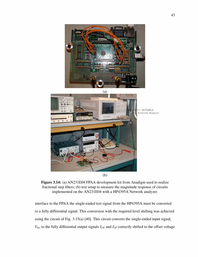
43

(a)

(b)

Figure 3.14: (a) AN231E04 FPAA development kit from Anadigm used to realizefractional step filters; (b) test setup to measure the magnitude response of circuits

implemented on the AN231E04 with a HP4395A Network analyzer.

interface to the FPAA the single-ended test signal from the HP4395A must be converted

to a fully differential signal. This conversion with the required level shifting was achieved

using the circuit of Fig. 3.15(a) [40]. This circuit converts the single-ended input signal,

Vin, to the fully differential output signals I1N and I1P correctly shifted to the offset voltage

44

V MRC with a gain of R f /Ri, described by the equations below

I1N = VinR f

Ri+V MRC (3.29)

I1P = �✓

VinR f

Ri+V MRC

◆(3.30)

Note that V MRC was generated internally by the FPAA and had a value of +1.5V in our

test setup. After the signal processing on the FPAA, the signals are output as differential

signals. To interface these signals with the HP4395A requires a conversion from the

differential to single-ended signals, achieved using the circuit of Fig. 3.15(b) [40]. This

circuit converts the differential input signals O1N and O1P to the single-ended output

signal Vo with a gain of R f /Ri described by the equation below

Vo =R f

Ri(O1P �O1N) (3.31)

Both the single-to-differential and differential-to-single circuits were realized using

TLE2072 op amps from Texas Instruments [41]. The components were selected to

maintain a gain of 1, with 5% tolerance resistors of 5.1kW and 100kW used to build the

single-to-differential and differential-to-single circuits, respectively. The block diagram

illustrating this test setup is shown in Fig. 3.16.

3.3.3.1 Experimental Low Pass Fractional Step Filters

The experimental results of the magnitude and phase responses of the approximated first

order FLPFs with fractional steps of 0.1, 0.5, and 0.9 are shown in Fig. 3.17 as dashed

lines along with the MATLAB simulation results of the theoretical transfer functions pre-

sented as solid lines. The experimental results show close agreement with the simulations

confirming the operation of the approximated FLPFs on the FPAA. This further verifies the

results of previous realizations of the approximated fractional step filter, supporting that

integer order filters can accurately approximate the incremental stepping of a FLPF. Com-

45

+

-

+

-

(a)

+

-

(b)

Figure 3.15: Circuits to realize the (a) level-shifting, single-to-differential and (b)differential-to-single signal conversions to interface the AN231 FPAA with the HP4395A

network analyzer.

paring the results, we find that the passband attenuation of the experimental and simulated

filters are very close to their theoretical values of �20(1+a)dB/decade. For compari-

son, these attenuations are listed in Table 3.9. The experimental results of the magnitude

and phase responses of the approximated fourth order FLPFs with fractional steps of 0.1,

46

Level-Shifting

Single-to-Differential

Converter

AN231E04 FPAA

Development Board

Differential-to-Single

Converter

HP4395A Network Analyzer

Figure 3.16: Block diagram of test setup with conversion circuits required to interface theAN231 FPAA and the HP4395A network analyzer.


1.1 �22 �21.34 �21.331.5 �30 �30.75 �30.611.9 �38 �38.81 �39.00

Table 3.9: Theoretical, simulated, and experimental stopband attenuations ofapproximated (1+a) order FLPF realized using FPAA.

0.5, and 0.9 are given in Fig. 3.18 as dashed lines along with the MATLAB simulation

results of the theoretical transfer functions presented as solid lines. The experimental re-

sults once again show close agreement with the simulations confirming that the method

of implementing a higher order FLPF by dividing the first order FLPF by a higher or-

der Butterworth polynomial is valid. It also validates that this method of implementing a

higher order filter maintains the fractional step through the stopband without the passband

peaking of previous fractional filters. Comparing the results, we find that the passband at-

tenuation of the experimental and simulated filters are very close to their theoretical values

of �20(4+a)dB/decade. For comparison, these attenuations are listed in Table 3.9. The

complete set of experimental and simulation results for fractional low pass filters are pre-

sented in Appendix A for the cases (n+a) when n = 1 to 4 in fractional steps of a = 0.1,

0.5, and 0.9.

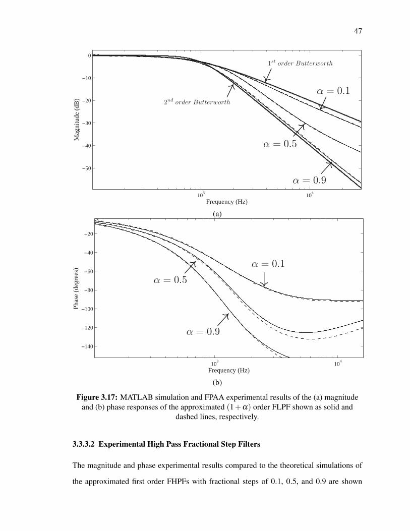
47

103

104

−50

−40

−30

−20

−10

0

Frequency (Hz)

Mag

nit

ud

e (d

B)

(a)

103

104

−140

−120

−100

−80

−60

−40

−20

Frequency (Hz)

Phas

e (d

egre

es)

(b)

Figure 3.17: MATLAB simulation and FPAA experimental results of the (a) magnitudeand (b) phase responses of the approximated (1+a) order FLPF shown as solid and

dashed lines, respectively.

3.3.3.2 Experimental High Pass Fractional Step Filters

The magnitude and phase experimental results compared to the theoretical simulations of

the approximated first order FHPFs with fractional steps of 0.1, 0.5, and 0.9 are shown

48

103

−70

−60

−50

−40

−30

−20

−10

0

Frequency (Hz)

Mag

nit

ud

e (d

B)

(a)

102

103

−400

−350

−300

−250

−200

−150

−100

−50

Frequency (Hz)

Phase (

degre

es)

(b)

Figure 3.18: MATLAB simulation and FPAA experimental results of the (a) magnitudeand (b) phase responses of the approximated (4+a) order FLPF shown as solid and


in Fig. 3.19 as dashed and solid lines, respectively. The experimental results show close

agreement with the simulations confirming that the use of the highpass to lowpass trans-

formation on the proposed transfer function (3.2) does realize a highpass filter without

49


4.1 �82 �81.39 �80.804.5 �90 �90.76 �90.404.9 �98 �98.3 �96.80

Table 3.10: Theoretical, simulated, and experimental stopband attenuations ofapproximated (4+a) order FLPF realized using FPAA.


1.1 �22 �21.43 �21.201.5 �30 �29.49 �29.801.9 �38 �37.09 �37.58

Table 3.11: Theoretical, simulated, and experimental stopband attenuations ofapproximated (1+a) order FHPF realized using FPAA.

passband peaking while maintaining the fractional step through the stopband. It also vali-

dates that the values of k2,3 for minimum passband error from the lowpass case also yield

a flat passband after the LP-to-HP transformation. Comparing the results, we find that

the passband attenuation of the experimental and simulated filters are very close to their

theoretical values of �20(1+a)dB/decade. These attenuations are listed in Table 3.11.

The experimental results of the magnitude and phase responses of the approximated

fourth order FHPFs with fractional steps of 0.1, 0.5, and 0.9 are shown in Fig. 3.20, as

dashed lines, with the MATLAB simulation results of the theoretical transfer functions

presented as solid lines. The experimental results show close agreement with the simu-

lations confirming that the method of implementing a higher order FHPF by dividing the

first order FHPF by a higher order Butterworth polynomial after the lowpass to highpass

transformation is successful. Also, that this method of implementing a higher order filter

maintains the fractional step through the stopband without the passband peaking of previ-

ous fractional filters. The passband attenuation of the experimental and simulated filters

are very close to their theoretical values of �20(4+a)dB/decade, listed in Table 3.12.

50

103

104

105

−60

−50

−40

−30

−20

−10

0

Frequency (Hz)

Mag

nit

ud

e (d

B)

(a)

103

104

−350

−300

−250

−200

Frequency (Hz)

Phas

e (d

egre

es)

(b)

Figure 3.19: MATLAB simulation and FPAA experimental results of the (a) magnitudeand (b) phase responses of the approximated (1+a) order FHPFs shown as solid and


3.3.4 Application of a Fractional Step Filter

To highlight the precise filtering achieved by a fractional step filter, two tones added using

the circuit in Fig. 3.21 are applied to approximated highpass filters of orders (4+a) =

51

104

−70

−60

−50

−40

−30

−20

−10

0

Frequency (Hz)

Mag

nit

ud

e (d

B)

(a)

104−300−250−200−150−100−50

050

(b)

Figure 3.20: MATLAB simulation and FPAA experimental results of the (a) magnitudeand (b) phase responses of the approximated (4+a) order FHPFs shown as solid and


4.1 to 4.9 in steps of 0.2 with the output of the filter measured by a HP4395A Spectrum

analyzer to determine the output signal power. The output of this topology is proportional

52


4.1 �82 �81.43 �80.44.5 �90 �89.1 �89.64.9 �98 �98.74 �99.2

Table 3.12: Theoretical, simulated, and experimental stopband attenuations ofapproximated (4+a) order FHPF realized using FPAA.

+

-

Figure 3.21: Op amp topology with output voltage proportional to the sum of the inputvoltages .

to the sum of the input voltages, described as

Vo =�✓

R3

R1V1 +

R3

R2V2

◆(3.32)

Which if R1 = R2 = R3 reduces to

Vo =�(V1 +V2) (3.33)

This circuit was realized using MC1458 op amps and 1% tolerance, 1kW resistors. Tones

at 3kHz and 10kHz with peak-to-peak voltages of 500mV are applied to the approximated

FHPFs shifted to a frequency of fo = 10kHz. The peak value of the tones for each filter

are presented in Table 3.13. Note that the use of the approximated fractional Laplacian

operator results in the deviation of the linear spacing between the powers of the tone at 3kHz

53

Order (n+a) Power @ 3kHz (dBm) Power @ 10kHz (dBm)

4.1 �32.7 3.944.3 �35.9 3.374.5 �38.2 3.54.7 �38.4 5.014.9 �40.7 4.45

Table 3.13: Signal power of tones at 3kHz and 10kHz after application to approximatedFHPFs of orders (4+a) = 4.1 to 4.9 in steps of 0.2

as a increases. This control of the attenuation is not possible using integer order filters.

Highpass Butterworth filters, frequency shifted to fo = 10kHz, would result in signals of

�32.5dBm and �43.4dBm for a 3kHz tone using 4th and 5th order filters, respectively. This

precise control is also shown in the frequency spectrum of Fig. 3.22. The spectrum of the

4th and 5th order highpass Butterworth filters, as dotted and solid lines respectively, are

compared to that of a 4.5 order FHPF, shown as a dashed line. All of the filters maintain

the tone at 10kHz with the attenuation of the 4.5 order filter at 3kHz clearly between those

of the standard Butterworth filters. These results reinforce the experimental results of the

magnitude response in Fig. 3.20; showing that these filters can be used to precisely control

attenuation characteristics.

3.4 Summary

In this chapter we have presented the design process and equations to realize fractional step

filters with an operational amplifier implementation and FPAA hardware. Simulated and

physically realized integer order filters demonstrate the fractional step through the stopband

for both highpass and lowpass filters of orders (1+a) and (4+a) in steps of 0.1, 0.5, and

0.9. In all cases the close agreement between the simulated and experimental results can

be observed. These results serve to verify that the lowpass to highpass transformation does

yield a highpass fractional step filter without peaking in the passband and that the selection

of k2,3 for minimum passband error also applies to the FHPFs. It also demonstrates that

the method for implementing higher order fractional step filters is suitable for both low and

54

Figure 3.22: Frequency spectrum of approximated 4.5 order FHPF (dashed) compared to4th (dotted) and 5th (solid) order highpass Butterworth filters.

high pass filters.

CHAPTER 4

EQUAL RIPPLE FRACTIONAL LAPLACIAN APPROXIMATION

In Chapter 1 applications of the fractional Laplacian operator in numerous areas of en-

gineering were presented. These concepts in circuit theory have applications in power

electronics [12], integrator [13, 14] and differentiator circuits [15], oscillators [16], multi-

vibrator circuits [17], and filter theory [18–21]. However, because there are no commercial

fractance devices available, integer order approximations of sa must be used to implement

systems that take advantage of fractional behaviour. There exist many methods to create

approximations of sa with varying order and accuracy; the accuracy and approximated fre-

quency band increasing as the order increases. In this chapter we present a method for

modifying a second order approximation of the fractional Laplacian operator that yields

an equal ripple approximation that has both lower peak and lower cumulative error when

compared to the original.

Previous work on the approximation of the general fractional Laplacian operator yielded

(3.1), a second order approximation using a CFE method [32] as

sa ⇡ (a2 +3a +2)s2 +(8�2a2)s+(a2 �3a +2)(a2 �3a +2)s2 +(8�2a2)s+(a2 +3a +2)

(4.1)

Repeated here as equation (4.1). Fig. 4.1 outlines the magnitude and phase of (4.1) com-

pared with sa when a = 0.7. From this figure, the magnitude error of the approximation

compared to the ideal case does not exceed 1.482dB for w e [0.0295,33.91]rad/s, while

the phase error does not exceed 3.155� for w e [0.1384,7.227]rad/s. We note also both the

56

10−2

10−1

100

101

102−40

−20

020

40

Frequency (rad/s)

Mag

nit

ud

e (

dB

)

10−2

10−1

100

101

1020

20

40

60

Frequency (rad/s)

Phase (

deg

rees)

Figure 4.1: Magnitude and phase of ideal (solid) and 2nd order approximation (dashed)of sa when a = 0.7.

magnitude and phase responses have inner and outer ripples, highlighted in Fig. 4.1.

To compare the peaks of the inner and outer ripples for both the magnitude and phase,

let us define an error, E, which is the difference between the ideal sa and (4.1) as

E = sa � (a2 +3a +2)s2 +(8�2a2)s+(a2 �3a +2)(a2 �3a +2)s2 +(8�2a2)s+(a2 +3a +2)

(4.2)

Using (4.2) the peaks of the magnitude and phase ripple errors can be calculated numeri-

cally, as shown in Fig. 4.2, for a where 0 < a < 1. From Fig. 4.2 it can be seen that both

the inner and outer ripple errors vary significantly with a . Noting that the size of the outer

ripple is always larger than the inner ripple for all values of a and that the maximum error

for magnitude and phase occur at different values of a. The magnitude error reaching a

maximum of 1.496dB when a = 0.65 with an inner ripple of 0.243dB, and the phase error

reaching a maximum of 3.211� when a = 0.54 with an inner ripple of 1.404�.

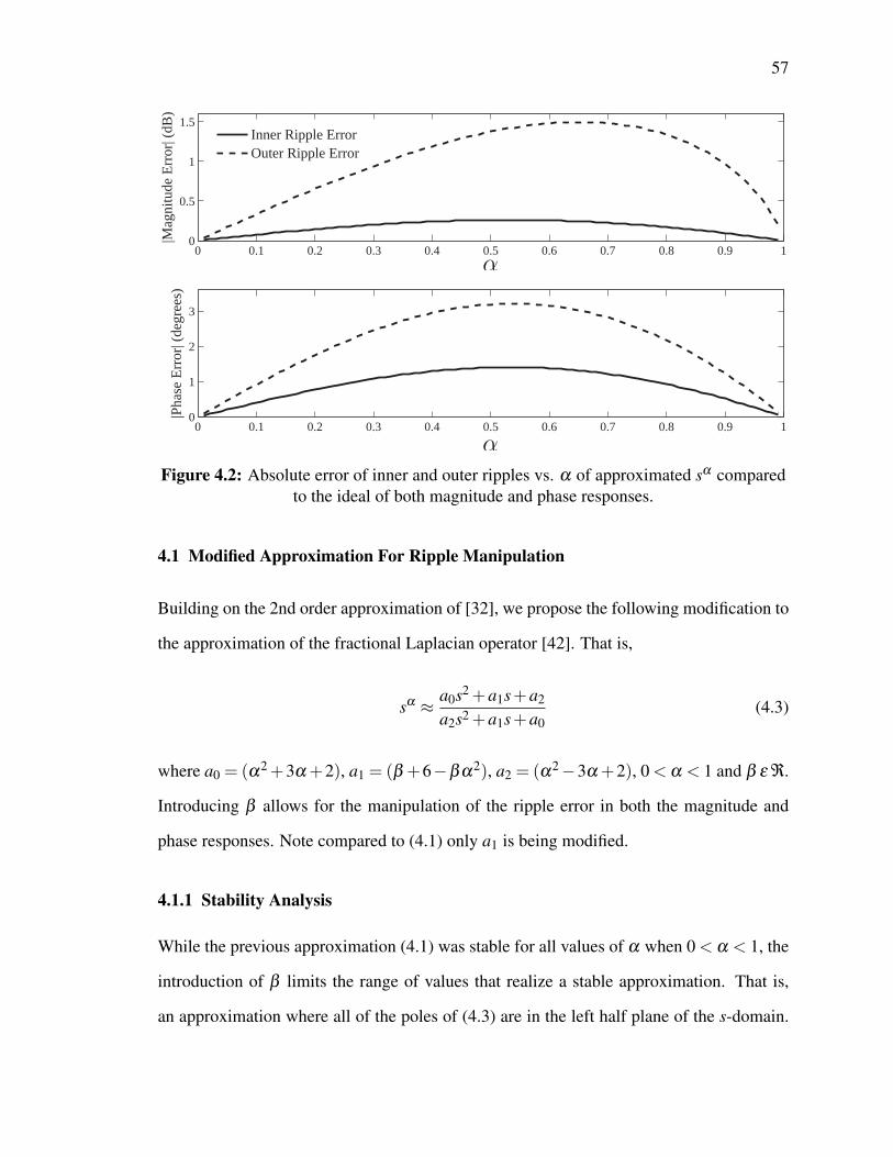
57

0 0.1 0.2 0.3 0.4 0.5 0.6 0.7 0.8 0.9 10

1

2

3

|Ph

ase

Err

or|

(d

egre

es)

0 0.1 0.2 0.3 0.4 0.5 0.6 0.7 0.8 0.9 1

0

0.5

1

1.5

|Mag

nit

ud

e E

rro

r| (

dB

)

Inner Ripple Error

Outer Ripple Error

Figure 4.2: Absolute error of inner and outer ripples vs. a of approximated sa comparedto the ideal of both magnitude and phase responses.

4.1 Modified Approximation For Ripple Manipulation

Building on the 2nd order approximation of [32], we propose the following modification to

the approximation of the fractional Laplacian operator [42]. That is,

sa ⇡ a0s2 +a1s+a2

a2s2 +a1s+a0(4.3)

where a0 = (a2+3a +2), a1 = (b +6�ba2), a2 = (a2�3a +2), 0 < a < 1 and b e ¬.

Introducing b allows for the manipulation of the ripple error in both the magnitude and

phase responses. Note compared to (4.1) only a1 is being modified.

4.1.1 Stability Analysis

While the previous approximation (4.1) was stable for all values of a when 0 < a < 1, the

introduction of b limits the range of values that realize a stable approximation. That is,

an approximation where all of the poles of (4.3) are in the left half plane of the s-domain.

58

These poles, s1,2 are calculated as

s1,2 =�a1 ±

qa2

1 �4a0a2

2a0(4.4)

Hence, to maintain the poles in the left half plane requires that s1,2 < 0, which is always

true if the following conditions are met

a1 > 0 (4.5)

�a1 +p(a�4aoa2 < 0 (4.6)

Substituting the values of a0,1,2 into (4.6) yields

4a4 �20a2 +16 > 0 (4.7)

Which is true over the regions a = (�•,2)[ (�1,1)[ (2,•). Therefore, the condition of

(4.6) is always met because a is defined as 0 < a < 1 which falls entirely within a region

where the inequality is always evaluated true. Substituting the value of a1 into (4.5) and

solving for b yields

b >�6

1�a2 (4.8)

Therefore to maintain stability, the value of b to manipulate the error ripple must be greater

than the value of (4.8) for the select value of a . Note that the value of b required for

stability decreases as a increases. The boundary between stable and unstable b values

from (4.8) for 0 < a < 1 is shown in Fig. 4.3. In the following sections we examine

how this modification can be used to manipulate the error of the response and evaluate the

cumulative error.

59

0.1 0.2 0.3 0.4 0.5 0.6 0.7 0.8 0.9

−300

−250

−200

−150

−100

−50

Figure 4.3: Minimum b required for stability of (4.3) for 0 < a < 1.

4.1.2 Error Ripple Manipulation

Using (4.3) the size of both the inner and outer error ripples in both the magnitude and phase

responses can be changed by modifying the value of b . Increasing b decreases the size of

the outer ripple error while increasing the inner ripple error in both the magnitude and phase

responses. Looking at the case when b = 2 in Fig. 4.4, when the modified approximation

(4.3) is equal to the original approximation (4.1), we see that the outer ripple error of the

magnitude response is 1.481dB with an inner ripple error of 0.225dB; while error ripples of

the phase response are 2.818� and 1.217� for the outer and inner error ripples, respectively.

Note that increasing b to 3 and 4 increases the inner ripple of the magnitude response to

0.5428dB and 0.8812dB, respectively; with the outer ripples decreasing to 1.027dB and

0.6054dB, respectively. The same behaviour is mirrored in the phase response, with inner

ripple values of 4.697� and 7.836� and outer ripple values of 1.458� and 0.4265� for b = 3

and b = 4, respectively.

4.1.3 Equi-Ripple Approximation

With the ability to increase the size of the inner ripple while decreasing that of the outer

ripple, there exists a value of b that will yield an equi-ripple error response of either the

60

10−2

10−1

100

101

0

0.5

1

1.5

Frequency (rad/s)

|Mag

nit

ud

e E

rro

r| (

dB

)

10−1

100

101

0

2

4

6

8

Frequency (rad/s)

|Ph

ase

Err

or|

(D

egre

es)

Figure 4.4: Magnitude and phase absolute inner and outer ripple error of (4.3) comparedto the ideal sa for b values from 2 to 4 when a = 0.7.

phase or magnitude for a given a . That is, a response where both the inner and outer

ripple errors are the same size. These values of b that yield this equi-ripple response,

for both magnitude and phase, using (4.3) were solved for numerically and are shown in

Fig. 4.5 for 0 < a < 1. Note that the values of b that create an equi-ripple response are

all positive and are therefore in the stable region. As a result, these values will result in

an approximation that is always stable. Also, from this data there is no intersection of

the values for magnitude and phase, so that it is never possible to have an approximation

with equi-ripple response in both magnitude and phase simultaneously. This equi-ripple

response for both magnitude and phase when a = 0.2 and a = 0.8 using b = 3.2907 and

b = 3.8382, respectively, for the magnitude response and b = 2.3626 and b = 2.3028,

respectively, for the phase response is shown in Fig. 4.6. Comparing the max ripple errors

from Fig. 4.6 for a = 0.2 and 0.8 to the values in Fig. 4.2 show a reduction in the max error

for both the magnitude and phase responses. For the case when a = 0.8, the max ripple

errors are 1.337dB and 2.173� for the magnitude and phase, respectively. Using the equi-

ripple b values in (4.3), those are b = 3.8382 and b = 2.3028 for magnitude and phase,

61

0 0.1 0.2 0.3 0.4 0.5 0.6 0.7 0.8 0.9 12

3

4

5

6

7

8

MagnitudePhase

Figure 4.5: b values required for equi-ripple magnitude (solid) and phase (dashed) errorapproximation for 0 < a < 1.

shows a reduction of the maximum error in both magnitude and phase when compared to

(4.1). Note the errors are reduced to 0.6542dB and 1.794� for the magnitude and phase

respectively, a reduction of 0.6828dB and 0.379�. This is also true when a = 0.2, using

the equi-ripple values, b = 3.2907 and b = 2.3626 for magnitude and phase, there is a

reduction of 0.2809dB and 0.266� in the maximum errors of the magnitude and phase,

respectively.

4.1.4 Cumulative Error

In order to quantify the error of both approximations to the ideal case, we use an objective

criteria [14] to compare them, defined as

CumulativeError =N

Âi=1

(Xi �Yi)2 (4.9)

where Xi is the approximation value of either phase or magnitude for a given frequency, Yi

is the ideal value for the same frequency value, and N is the number of samples for the com-

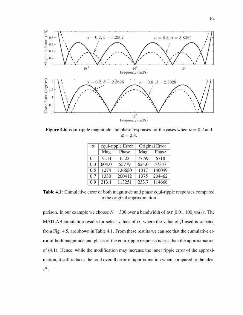
62

10−1

100

101

0

0.2

0.4

0.6

0.8

Frequency (rad/s)

|Mag

nit

ud

e E

rro

r | (

dB

)

100

0

0.5

1

1.5

2

Frequency (rad/s)

|Ph

ase

Err

or|

(d

egre

es)

Figure 4.6: equi-ripple magnitude and phase responses for the cases when a = 0.2 anda = 0.8.

a equi-ripple Error Original ErrorMag Phase Mag Phase

0.1 75.11 6523 77.59 67180.3 604.0 55779 624.0 573470.5 1274 136650 1317 1400490.7 1330 200412 1375 2044620.9 213.1 113251 233.7 114666

Table 4.1: Cumulative error of both magnitude and phase equi-ripple responses comparedto the original approximation.

parison. In our example we choose N = 300 over a bandwidth of w e [0.01,100]rad/s. The

MATLAB simulation results for select values of a , where the value of b used is selected

from Fig. 4.5, are shown in Table 4.1. From these results we can see that the cumulative er-

ror of both magnitude and phase of the equi-ripple response is less than the approximation

of (4.1). Hence, while the modification may increase the inner ripple error of the approxi-

mation, it still reduces the total overall error of approximation when compared to the ideal

sa .

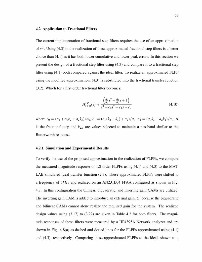
63

4.2 Application to Fractional Filters

The current implementation of fractional-step filters requires the use of an approximation

of sa . Using (4.3) in the realization of these approximated fractional step filters is a better

choice than (4.1) as it has both lower cumulative and lower peak errors. In this section we

present the design of a fractional step filter using (4.3) and compare it to a fractional step

filter using (4.1) both compared against the ideal filter. To realize an approximated FLPF

using the modified approximation, (4.3) is substituted into the fractional transfer function

(3.2). Which for a first order fractional filter becomes:

HLP1+a(s)⇡

⇣a2a0

s2 + a1a0

s+1⌘

s3 + c0s2 + c1s+ c2(4.10)

where c0 = (a1 + a0k2 + a2k3)/a0, c1 = (a1(k2 + k3)+ a2)/a0, c2 = (a0k3 + a2k2)/a0, a

is the fractional step and k2,3 are values selected to maintain a passband similar to the

Butterworth response.


To verify the use of the proposed approximation in the realization of FLPFs, we compare

the measured magnitude response of 1.8 order FLPFs using (4.1) and (4.3) to the MAT-

LAB simulated ideal transfer function (2.3). These approximated FLPFs were shifted to

a frequency of 1kHz and realized on an AN231E04 FPAA configured as shown in Fig.

4.7. In this configuration the bilinear, biquadratic, and inverting gain CAMs are utilized.

The inverting gain CAM is added to introduce an external gain, G, because the biquadratic

and bilinear CAMs cannot alone realize the required gain for the system. The realized

design values using (3.17) to (3.22) are given in Table 4.2 for both filters. The magni-

tude responses of these filters were measured by a HP4395A Network analyzer and are

shown in Fig. 4.8(a) as dashed and dotted lines for the FLPFs approximated using (4.1)

and (4.3), respectively. Comparing these approximated FLPFs to the ideal, shown as a

64

Figure 4.7: FLPF implementation using the bilinear filter, biquadratic filter, and invertinggain CAMs of the AnadigmDesigner2 tools.

solid line in Fig. 4.8(a), both responses closely match the passband of the filter. Viewing

the pass and stopbands we see the differences between implementing the FLPFs using the

different approximations of sa . Through the passband we note a minimal difference from

400Hz to 900Hz where the original approximation more closely resembles the ideal case

than the equi-ripple approximation. Also, from approximately 1.6kHz to 4.2kHz using

the equi-ripple approximation results in a larger deviation compared to the ideal than the

original approximation; which is expected because the inner ripple error of the approxi-

mation increases using the equi-ripple response compared to the original. However, from

approximately 4.2kHz to 42kHz the modified approximation is a closer approximation of

(2.3) than the original modification, highlighted in the inset of Fig. 4.8(a), a result of the

reduced outer ripple error. Therefore, while using (4.3) increases the error of the approx-

imated FLPF over small ranges it also decreases the error over a much larger range in the

stopband. This illustrates that the use of the equi-ripple approximation over the original

approximation is a better choice in the implementation of FLPFs. The step response of the

1.8 order filter was also investigated to confirm its stability, and is shown in Fig. 4.8(b).

The magnitude responses using the equi-ripple magnitude approximation (4.10) for fil-

ters of order (1+a) for the cases a = 0.2, 0.5, and 0.8 using the values of k2,3 from Fig.

2.1 were both simulated using MATLAB and realized using an Anadigm 231E04 FPAA

using the same configuration of the bilinear, biquadratic, and inverting gain CAMs of Fig.

4.7. For these filters the pole and zero frequencies were shifted from the normalized value

65

102

103

104

−50

−40

−30

−20

−10

0

Frequency (Hz)

Mag

nit

ud

e (d

B)

(a)

(b)

Figure 4.8: Ideal and approximated magnitude responses of (1+a) = 1.8 order FLPFsusing (4.1) and (4.3) as solid, dashed, and dotted lines, respectively. Note that for all

FLPFs k2 = 1.11 and k3 = 0.966 with b = 3.8382 in (4.3). (b) Step response ofapproximated 1.8 order FLPF using (4.3).

66

Order (1+0.8)Design Value Original Modified

f1(kHz) 0.611 0.504f2p(kHz) 1.30 1.42f2z(kHz) 4.61 4.60

Q2p 0.674 0.672Q2z 0.163 0.149G1,2 1 1G 0.0795 0.0963

Table 4.2: Realized CAM values for physical implementation of the 1.8 order FLPFsrealized using the original and equi-ripple approximation, (4.1) and (4.3), respectively.

Note b = 3.8382 for the equi-ripple magnitude approximation.

Order (1+a)k2k3

1.20.3080.852 1.50.594

0.912 1.81.1100.968


Q2p 0.4667 0.467 0.6032 0.612 0.6722 0.672Q2z 0.2129 0.215 0.1958 0.197 0.1490 0.149G1,2 1 1 1 1 1 1G 1.8442 1.84 0.5149 0.515 0.0964 0.0963

Table 4.3: Realized CAM values for physical implementation of the approximated FLPFsusing equi-ripple magnitude approximation. Note b = 3.2907, 3.4199, and 3.8382 for

(1+a) = 1.2, 1.5, and 1.8, respectively.

of 1rad/s to 6283rad/s or 1kHz. The theoretical and realized FPAA values for the imple-

mentation of filters of order (1+a) = 1.2, 1.5, and 1.8 are given in Table 4.3. The results

are shown in Fig. 4.9(a) as solid and dashed lines for the theoretical and experimental re-

sults, respectively. Again, the simulated and experimental results show close agreement

with the theoretical, simulated, and experimental stopband attenuations given in Table 4.4.

These results verify that the use of our proposed second order approximation of the frac-

tional Laplacian operator is both valid and stable for the implementation of approximated

fractional step filters.

67

103

104

−50

−40

−30

−20

−10

0

Frequency (Hz)

Mag

nit

ud

e (d

B)

Figure 4.9: Measured and MATLAB simulation results of the magnitude response of theapproximated (1+a) order FLPF, shown as dashed and solid lines, respectively.


1.2 �24 �24.07 �24.021.5 �30 �29.34 �31.401.8 �36 �37.63 �38.42

Table 4.4: Theoretical, simulated, and experimental stopband attenuations of (1+a)order FLPF approximated with equi-ripple approximation realized using an FPAA.

4.3 Summary

In this chapter we present a modification to the 2nd order approximation of the fractional

Laplacian operator obtained through the CFE method [32]. With this modification we are

able to manipulate the error ripples of the approximation, showing that we can create an

equal ripple error response in either magnitude or phase of the approximation. This equal

ripple response has both lower cumulative error and peak error when compared to the orig-

inal approximation. The stability of the modified approximation is examined and shown

68

to be stable for all the values that yield an equal ripple approximation in both phase and

magnitude. A 1.8 order FLPF using the equi-ripple approximation compared to the original

approximation realized on an FPAA is presented to show the advantage of using this ap-

proximation in the realization of fractional filters. Low pass filters or orders (1+a) = 1.2,

1.5, and 1.8 are also presented with the simulation results showing close agreement with

the experimental results while also illustrating that the filter is stable.

CHAPTER 5

TOW-THOMAS BIQUAD REALIZED WITH FRACTIONAL CAPACITOR

Currently there are no commercial fractional capacitors, devices with an impedance Z(s) =

1/Csa where 0 < a < 1, available for the physical implementation of fractional order

circuits. However, there are still reported physical implementations of such devices [8,

43–46] using fractal shapes. A fractal is “a rough or fragmented geometric shape that

can be split into parts, each of which is (at least approximately) a reduced-sized copy of

the whole” [47]. Fractals such as the Sierpinski [48], Tree [43, 45], Hilbert [8], Koch

and Peano [46] structures, when implemented as one of the plates in a capacitor, have

been shown to exhibit fractional order electrical impedances. These fractional capacitors

(FCs) can be used in the realization of fractional systems without an approximation of the

fractional Laplacian operator. In this section we explore the application of two such devices

which were provided to us on loan by Prof. Théodore Cisse Haba from the Département

Génie Electrique et Electronique at the Institut National Polytechnique in Yamoussoukro,

Côte d’Ivoire. These two fractional capacitors are shown in Fig. 5.1(a), labelled as Hilbert

and Arbre, with their fractal structures shown in Fig. 5.1(b) and (c), respectively, with

capacitances of 6.5nF and 1.5nF with a = 0.5, respectively [8, 43]. These devices open

the door to practical applications involving fractional order systems. Using these elements

in traditional continuous time filters we can explore the benefits that accompany the use of

fractional capacitors in filter circuits.

70

(a)

(b)

(c)

Figure 5.1: (a) Packaged fractional capacitors implemented using photolithographicfractal structures on silicon, based on the (b) Hilbert and (c) Tree fractal structures.

71

+

+

+

-

-

-

Figure 5.2: Tow-Thomas biquad topology.

5.1 Tow-Thomas Biquad

The Tow-Thomas biquad [49–51] of Fig. 5.2 is an active-RC topology used to realize

both lowpass and bandpass biquadratic filtering functions. This topology has been widely

used because it is simple, versatile, requires few components, and has very low sensitivities

to changes in the passive RC components and gains of the operational amplifiers [49].

Analysis of this biquad yields the lowpass and bandpass functions

V LPo (s)

Vin(s)= �

R6R1R4R5C1C2

s2 + sR3C1

+ R6R2R4R5C1C2

(5.1)

V BPo (s)

Vin(s)= �

s 1R1C1

s2 + sR3C1

+ R6R2R4R5C1C2

(5.2)

The Tow-Thomas biquad can be used to implement a 2nd order low pass Butterworth

response through selecting the appropriate resistor and capacitor values to realize the de-

sired cutoff frequency, wo, and quality factor, Q, associated with this response. The design

equations to determine the component values are

wo =1p

R2R4C1C2(5.3)

Q =R3C1

wo(5.4)

72

which when we set C1 = C2 = C and R2 = R4 = R and R5 = R6 for simplicity (5.3) and

(5.4) become

wo =1

RC(5.5)

Q =R3

R(5.6)

5.1.1 Fractional Tow-Thomas Biquad

While the traditional Tow-Thomas Biquad uses standard capacitors, it is possible to replace

a capacitor in the system with a fractional capacitor. This approach of replacing traditional

capacitors with fractional capacitors has previously been investigated for both the Sallen-

Key filter and Kerwin-Huelsman-Newcomb biquad [19]. Here, we replace C2 in the Tow-

Thomas Biquad with a fractional capacitor of impedance ZC2 =1

saC2, which modifies the

transfer function at the low pass filter node to

V LPo (s)

Vin(s)=�

1R1R4C1C2

s1+a + saR3C1

+ 1R2R4C1C2

(5.7)

Effectively realizing a fractional step low pass transfer function of order (1+a). Note

that (5.7) is of the form of (2.3) when n = 1 after apply the frequency shift transformation

s = swo

, where wo is the denormalized frequency in rad/s. Applying this transformation

(2.3) becomes

HLP1+a(s) =

k1w1+ao

s1+a + k2wosa + k3w1+ao

(5.8)

73

ValueComponent Fig. 5.2

C1, C2 6.8nFR1, R2, R4, R5, R6 46.8kW

R3 33.1kW

Table 5.1: Component values to realize 2nd order Butterworth LP response with cutofffrequency of 500Hz using the Tow-Thomas Biquad.

Comparing coefficients of (5.7) to (5.8) while ignoring the sign in (5.7) yields the following

relationships

k1 =1

R1R4C1C2w1+ao

(5.9)

k2 =1

R3C1wo(5.10)

k3 =1

R2R4C1C2w1+ao

(5.11)

Therefore, using equations (5.9) to (5.11) the fractional Tow-Thomas biquad can be used

to implement a frequency shifted (1+a) order FLPF of the form proposed in (2.3).

5.2 Simulation and Experimental Results

To initially test the fractional capacitors on loan to us, they were used to replace the ca-

pacitor C2 in the traditional Tow-Thomas biquad of Fig. 5.2, initially designed to realize

a 2nd order low pass Butterworth filter of quality factor Q = 1/p

2 and cutoff frequency

of fo = 500Hz or w0 = 3141.69rad/s. Using the design equations of (5.5) and (5.6) the

component values required for this realization are given in Table 5.1. This circuit was

breadboarded using MC1458 op amps (1MHz gain bandwidth product) with 5% tolerance

resistors and 20% tolerance capacitors. The magnitude response at the low-pass output

node was measured using the HP4395A Network analyzer.

The MATLAB simulations and experimental results of the Tow-Thomas biquad when

C2 = 6.8nF are shown in Fig. 5.3 labelled by ZC2 =1

s6.8nF as dotted and dashed lines,

74

103

104

−35

−30

−25

−20

−15

−10

−5

0

5

Frequency (Hz)

Mag

nit

ud

e (d

B)

Figure 5.3: Magnitude response of Tow-Thomas and fractional Tow-Thomas biquad lowpass function when a = 0.5 as solid and dashed lines, respectively.

respectively. The experimental results show perfect agreement with the simulations, con-

firming the operation of the realized 2nd order Butterworth filter using the Tow-Thomas.

The MATLAB simulations when C2 is replaced by fractional capacitors of values 6.5nF

and 1.5nF with a = 0.5, representing the expected values of the Hilbert and Arbre FCs,

are also shown in Fig. 5.3 as dashed lines labelled ZC2 =1

s0.56.5nF and ZC2 =1

s0.51.5nF , respec-

tively. These two responses both display the fractional step behaviour in the stopband with

attenuations of �30.12dB/dec and �30.52dB/dec very close to theoretical attenuation of

�20(1+0.5) =�30dB/dec. Note that the use of a fractional capacitor with characteristic

a = 0.5 with a capacitance close to that required for our implementation of the frequency

shifted 2nd order LP Butterworth filter, 6.5nF compared to 6.8nF , results in the �3dB fre-

quency increasing from 500Hz to 11.1kHz. To realize this same �3dB frequency using a

traditional capacitor and the same resistor values would require a capacitor of 0.3064nF .

However, both the simulated magnitudes responses using FCs exhibit the undesired peak-

ing in the passband, which is a result of the poles moving closer to the imaginary axis and

the values of k2,3 not being optimized for minimum passband error.

75

The experimental magnitude responses at the LP output node of the realized Tow-

Thomas biquad when C2 was replaced by the the Hilbert and Arbre fractional capacitors

are given in Fig. 5.3 as dotted lines labelled, Hilbert FC and Arbre FC, respectively. Note

that the results for both FCs do not match the theoretical, indicating that how we model the

fractional capacitors in the simulations of our system was incorrect. The transfer function

(5.7) is based on the assumption that the fractional capacitor behaves as the ideal case; that

it is purely capacitive with no resistive components. However, the experimental results in

Fig. 5.3 indicate that this assumption was not valid. Further investigation into the Hilbert

FC indicated that it has a resistance in parallel with its fractional capacitor component, the

impedance model based on this parallel resistance is shown in Fig. 5.4(a). Using this model

in place of C2 in the Tow-Thomas biquad results in the circuit given in Fig. 5.4(b). The

transfer function of the fractional Tow-Thomas biquad at the LP output node, again when

R5 = R6 with the parallel resistance, Rp, becomes

V LPo (s)

Vin(s)=�

1R1R4C1C2

s1+a + s 1RpC2

+ sa 1R3C1

+R2R4+R3Rp

R2R3R4RpC1C2

(5.12)

Note that when (5.12) is compared to (5.7) there is an extra coefficient, s 1RpC2

, and the DC

gain coefficient changes. Therefore, using the fractional capacitor with a parallel resis-

tance we are not able to realize the transfer function of (2.3) which explains the difference

between the theoretical and experimental results using the Hilbert FC.

Conversely, through observation of the experimental results using the Arbre fractional

capacitor, it appeared to behave as an ideal fractional capacitor. As the slope of the stop-

band of the experimental results was parallel to the stopband of the simulated ideal case.

However, while the stopband was parallel to the ideal, the experimental pole frequency was

at a much lower frequency than expected by the reported 1.5nF capacitance of the device.

With the pole frequency occurring around 2�3kHz as opposed to the 20�30kHz expected

from the simulation. Therefore, it appears that the capacitance value of the Arbre FC used

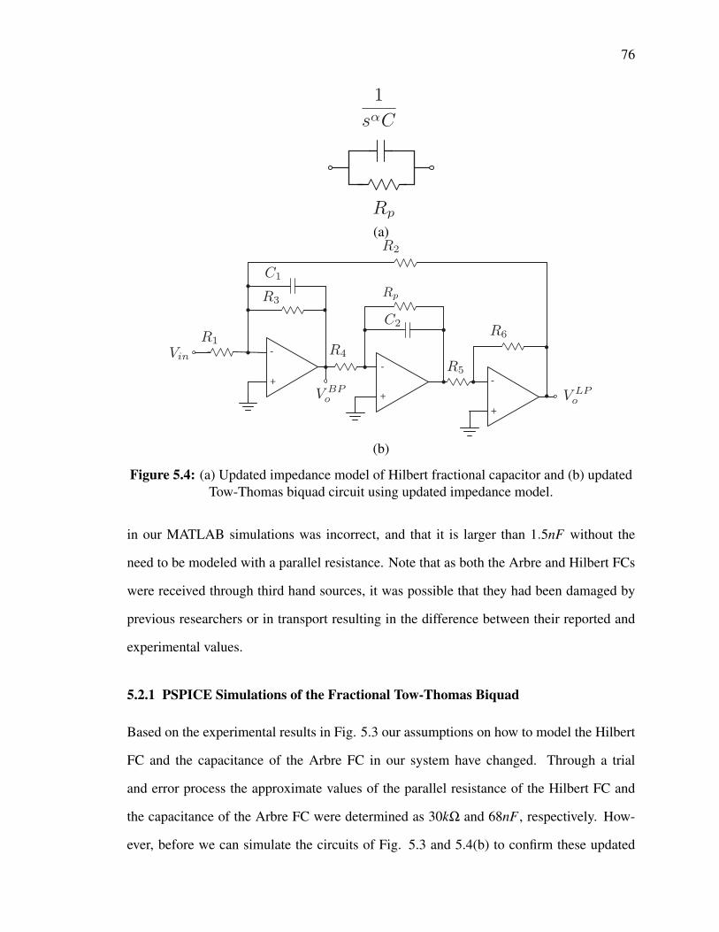
76

(a)

+

+

+

-

-

-

(b)

Figure 5.4: (a) Updated impedance model of Hilbert fractional capacitor and (b) updatedTow-Thomas biquad circuit using updated impedance model.

in our MATLAB simulations was incorrect, and that it is larger than 1.5nF without the

need to be modeled with a parallel resistance. Note that as both the Arbre and Hilbert FCs

were received through third hand sources, it was possible that they had been damaged by

previous researchers or in transport resulting in the difference between their reported and

experimental values.

5.2.1 PSPICE Simulations of the Fractional Tow-Thomas Biquad

Based on the experimental results in Fig. 5.3 our assumptions on how to model the Hilbert

FC and the capacitance of the Arbre FC in our system have changed. Through a trial

and error process the approximate values of the parallel resistance of the Hilbert FC and

the capacitance of the Arbre FC were determined as 30kW and 68nF , respectively. How-

ever, before we can simulate the circuits of Fig. 5.3 and 5.4(b) to confirm these updated

77

ValuesComponent 6.5nF 68nF

Ra 304.95kW 29.150kWRb 2.440MW 233.20kWRc 20.23MW 1.9335MWRd 690.12kW 66.024kWRe 1.0344MW 99.349kWCb 391.37pF 4.094nFCc 506.09pF 5.294nFCd 6.1042pF 638.59pFCe 215.60pF 2.2555nF

Table 5.2: Component values to realize approximated fractional capacitors of 6.5nF and68nF centered around 500Hz when a = 0.5 using RC ladder topology of inset in Fig. 5.5.

models, a fractional capacitor must be approximated that can be simulated using PSPICE.

The fractional capacitors required for these simulations were approximated using Carlson’s

method [29] to a second iteration and realized using the partial fraction decomposition

shown in the insets of Fig. 5.5. The values of resistors and capacitors used in the PSPICE

simulations of the fractional Tow-Thomas biqaud with the approximated FCs are given in

Table 5.1. These values realize approximated FCs of 6.5nF and 68nF with a = 0.5 cen-

tered around a frequency of 500Hz. The process and MAPLE code used to calculate the

component values to realize an approximated fractional capacitor for any capacitance, a ,

and center frequency are presented in Appendix B. Each of the circuits in Fig. 5.5 were

built and simulated in PSPICE using MC1458 op amps and the component values listed

in Tables 5.2 and 5.3. The experimental results compared to the PSPICE simulations of

the modified circuits are shown in Fig. 5.6 as dashed and solid lines, respectively, with the

results using the Hilbert and Arbre fractional capacitors labelled Hilbert FC and Arbre FC,

respectively. The simulations and experimental results show close agreement confirming

that our new assumptions regarding the modeling of the fractional capacitors are valid and

corroborating the fractional behaviour of the capacitors. This fractional behaviour is clearly

evident in the stopband attenuation using the Arbre fractional capacitor. With the attenua-

tion closely matching the theoretical �20(1+a)dB/dec in the stopband. For comparison

78

+

+

+-

-

-

(a)

+

+

+-

-

-

(b)

Figure 5.5: Fractional Tow-Thomas biquad with approximated fractional capacitorsrealized with RC ladders for PSPICE simulation of circuits with the (a) Arbre and (b)

Hilbert FCs.

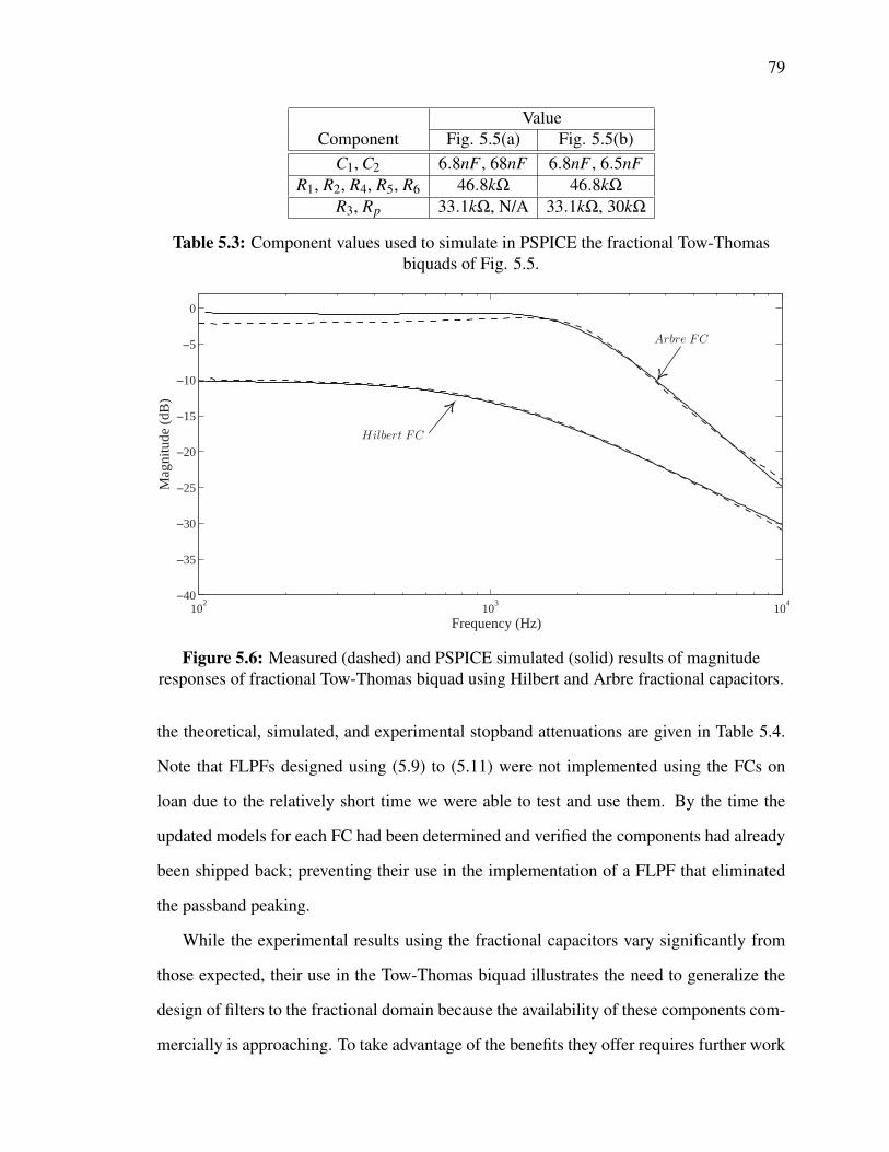
79

ValueComponent Fig. 5.5(a) Fig. 5.5(b)

C1, C2 6.8nF , 68nF 6.8nF , 6.5nFR1, R2, R4, R5, R6 46.8kW 46.8kW

R3, Rp 33.1kW, N/A 33.1kW, 30kW

Table 5.3: Component values used to simulate in PSPICE the fractional Tow-Thomasbiquads of Fig. 5.5.

102

103

104

−40

−35

−30

−25

−20

−15

−10

−5

0

Frequency (Hz)

Mag

nit

ude

(dB

)

Figure 5.6: Measured (dashed) and PSPICE simulated (solid) results of magnituderesponses of fractional Tow-Thomas biquad using Hilbert and Arbre fractional capacitors.

the theoretical, simulated, and experimental stopband attenuations are given in Table 5.4.

Note that FLPFs designed using (5.9) to (5.11) were not implemented using the FCs on

loan due to the relatively short time we were able to test and use them. By the time the

updated models for each FC had been determined and verified the components had already

been shipped back; preventing their use in the implementation of a FLPF that eliminated

the passband peaking.

While the experimental results using the fractional capacitors vary significantly from

those expected, their use in the Tow-Thomas biquad illustrates the need to generalize the

design of filters to the fractional domain because the availability of these components com-

mercially is approaching. To take advantage of the benefits they offer requires further work

80


1.5 �30 �31.6 �31.22

Table 5.4: Theoretical, simulated, and experimental stopband attenuations of fractionalTow-Thomas biquad realized with the Arbre fractional capacitor.

in the exploration and realization of fractional order circuits and systems.

5.3 Summary

In this chapter the use of fractional capacitors, with impedance Z(s) = 1/Csa where 0 <

a < 1, were used to create a fractional Tow-Thomas biquad. The effect of the fractional

capacitor on the �3dB frequency and stopband attenuation compared to the original are

shown through MATLAB simulations. Fractional capacitors realized using a photolitho-

graphic fractal structure on silicon [8, 43, 45] on loan were used in the implementation of

the fractional Tow-Thomas biquad. However, these fractional capacitors do not exhibit the

ideal fractional behaviour. Through modification of the modeling of these capacitors in

our system we are able to closely match the simulations to the experimental results. Using

these fractional capacitors we were able to realize fractional step filters without the use of

the approximated fractional Laplacian operator.

CHAPTER 6

CONCLUSIONS AND FUTURE WORK

6.1 Conclusion

Throughout this work we investigated three areas of research focus. First we investigated

the design and implementation of fractional step filters without the passband peaking of

previously proposed filters. Secondly, a modification of the approximated fractional Lapla-

cian operator to an equi-ripple error was proposed approximation. Finally, the use of actual

fractional capacitors in the fractional Tow-Thomas biquad was used to realize a fractional

step filter.

In the first area of research a new fractional low pass transfer function that maintains

the fractional step through the stopband while maintaining a flat passband was presented.

With the stability investigated we showed it is always stable for orders (1+a)< 2. Both a

method for the implementation of higher order filters and the lowpass to highpass transfor-

mations were presented. Simulations and physically realized integer order filters demon-

strate the fractional step through the stopband for both highpass and lowpass filters of

orders (1+a) and (4+a) in steps of 0.1, 0.5, and 0.9; all showing very close agreement

between the simulated and experimental results. These results verified that the lowpass to

highpass transformation does yield a highpass fractional step filter without peaking in the

passband, and that the selection of constants k2,3 for minimum passband error also applies

to the FHPFs, and the method for implementing higher order fractional step filters was

suitable for both low and high pass filters. This work presented the design process and

equations to realize fractional step filters with an operational amplifier implementation and

82

FPAA hardware.

In the second area of research a modification to a 2nd order approximation of the frac-

tional Laplacian operator obtained through the CFE method [32] was presented. Here we

showed that an equal ripple error response in either magnitude or phase of the approxi-

mation can be created. This equal ripple response has both lower cumulative error and

peak error when compared to the original approximation. The stability of the modified

approximation was examined and shown to be stable for all the values that yield an equal

ripple approximation in both phase and magnitude. Fractional low pass filters of order

(1+a) = 1.8 are realized using the modified and original approximations compared to the

ideal filter to highlight the benefit of the modified approximation and confirming its stabil-

ity. Fractional step filters of orders (1+a) = 1.2, 1.5, and 1.8 are also physically realized

on an FPAA to further validate the application of the approximation.

Finally, fractional capacitors realized using photolithographic fractal structures on sil-

icon [8, 43] were used in the implementation of a fractional Tow-Thomas biquad. Using

the fractional Tow-Thomas biquad we have implemented a fractional step low pass filter of

order (1+a) = 1.5 without the use of the approximated fractional Laplacian operator.

6.2 Contribution

The main contributions of this thesis have been to two areas. First in the creation of frac-

tional step filters that have a flat passband while maintaining the fractional step through

the stopband and secondly in the modification to the approximated fractional Laplacian

operator to create an equiripple error response.

The fractional step filter presented solves the problem of passband peaking previously

seen in other FLPFs. This is a further step in the process to create a more general filter de-

sign process through the import of concepts from fractional calculus. The design equations

and process to create fractional step low and highpass filters of any order are presented.

The realization of these filters using an approximation of the fractional Laplacian operator

83

shows how these filters can be physically implemented using integer order approximations

until such a time as general fractance devices are available. These physical filters verify

that these filters, 1) exhibit the fractional step stopband seen in the simulations, 2) that

the method to implement higher order fractional step filters is valid, and 3) the lowpass to

highpass transformation does create a fractional highpass filter.

The modification of the 2nd order approximated fractional Laplacian operator is benefi-

cial not just to the realization of approximated fractional step filters, but to any application

that requires the use of a fractional Laplacian operator. It shows both lower cumulative

and peak magnitude error over the orignal approximation, and was therefore a closer ap-

proximation to the ideal sa . Therefore its use in any application that requires the fractional

Laplacian operator would show closer agreement to the ideal case than the original approx-

imation.

6.3 Future Work

This work has focused on the importing of concepts from fractional calculus into the design

of filters to create fractional step filters with a flat passband in their magnitude response.

However, this is not the only filter type that could benefit from the use of the fractional

Laplacian operator. These principles could potentially be expanded to the Chebyshev, In-

verse Chebyshev, and Elliptic filter approximations to create fractional step filters with

equiripple stop and passbands. Also, work needs to be done to realize a true fractional

Butterworth filter, that maintains the �3dB frequency for all values of a .

The entirety of this work focused on the magnitude response of fractional step filters.

Leaving the field of the fractional behaviour of the phase response when using the fractional

Laplacian operator completely unexplored. Further work needs to be done to determine

how the phase can be manipulated. This could be further extended to the delay of filters as

well. This could potentially yield delay filters with a fractional step delay giving complete

control of the delay introduced; a very interesting possibility.

84

In regards to the modification of the fractional Laplacian operator, only a 2ndorder ap-

proximation was explored. Work could be done to determine if these results could be

expanded to higher order approximations; that could yield higher order equal ripple ap-

proximations with lower cumulative and peak errors.

With fractional capacitors showing the potential to become commercially available the

exploration of circuit topologies, that make use of these fractional behaviours, needs to be

further explored.

BIBLIOGRAPHY

[1] A. I. Zverev, Handbook of Filter Synthesis. New York: John Wiley and Sons, 1967.

1, 18

[2] L. P. Huelsman, Active and Passive Analog Filter Design: An Introduction. McGraw-

Hill, Inc., 1993. 2, 3, 25

[3] K. Oldham and J. Spanier, The Fractional Calculus: Theory and Applications of Dif-

ferentiation and Integration to Arbitrary Order. New York: Academic Press, 1974.

4, 5

[4] K. Miller and B. Ross, An introduction to the fractional calculus and fractional dif-

ferential equations. John Wiley and Sons, 1993. 4

[5] S. Samko, A. Kilbas, and O. Marichev, Fractional integrals and derivatives: theory

and application. Gordon and Breach, 1987. 4

[6] M. Ortigueira, “An introduction to the fractional continuous-time linear systems: the

21st century systems,” IEEE Circuits Syst. Mag., vol. 8, no. 3, pp. 19 – 26, Third

Quarter 2008. 5

[7] I. Podlubny, I. Petras, B. Vinagre, P. O’Leary, and L. Dorcak, “Analogue realizations

of fractional-order controllers,” Nonlinear Dynamics, vol. 29, pp. 281–296, 2002. 5,

21, 22

86

[8] T. Haba, G. Loum, J. Zoueu, and G. Ablart, “Use of a component with fractional

impedance in the realization of an analogical regulator of order 1/2,” J. Applied Sci-

ences, vol. 8, no. 1, pp. 59 – 67, Jan. 2008. 5, 69, 80, 82

[9] J. Machado, I. Jesus, A. Galhano, and J. Cunha, “Fractional order electromagnetics,”

Signal Processing, vol. 86, no. 10, pp. 2637 – 44, Oct. 2006. 5

[10] F. Miguel, M. Lima, J. Machado, and M. Crisostomo, “Experimental signal analysis

of robot impacts in a fractional calculus perspective,” J. of Advanced Computational

Intelligence and Intelligent Informatics, vol. 11, p. 1079, 2007. 5

[11] N. F. Ferreira, F. Duarte, M. Lima, M. Marcos, and J. T. Machado, “Application of

fractional calculus in the dynamical analysis and control of mechanical manipulators,”

Fractional Calculus and Applied Analysis, vol. 11, no. 1, pp. 91–113, 2008. 5

[12] A. Calderon, B. Vinagre, and V. Feliu, “Fractional order control strategies for power

electronic buck converters,” Signal Processing, vol. 86, no. 10, pp. 2803 – 19, Oct.

2006. 5, 55

[13] P. Varshney, M. Gupta, and G. Visweswaran, “New switched capacitor fractional or-

der integrator,” J. of Active and Passive Electronic Devices, vol. 2, pp. 187–197, 2007.

5, 55

[14] G. Santamaria, J. Valverde, R. Perez-Aloe, and B. Vinagre, “Microelectronic imple-

mentations of fractional-order integrodifferential operators,” J. Comput. Nonlinear

Dyn., vol. 3, no. 2, p. 021301 (6 pp.), Apr. 2008. 5, 55, 61

[15] K. Biswas, S. Sen, and P. K. Dutta, “Realization of a constant phase element and its

performance study in a differentiator circuit,” IEEE Trans.s on Circuits and Syst. II:

Express Briefs, vol. 53, no. 9, pp. 802 – 806, 2006. 5, 55

87

[16] W. Ahmad, R. Ei-Khazali, and A. Elwakil, “Fractional-order wien-bridge oscillator,”

Electron. Lett. (UK), vol. 37, no. 18, pp. 1110 – 12, Aug. 2001. 5, 55

[17] B. Maundy, A. Elwakil, and S. Gift, “On a multivibrator that employs a fractional

capacitor,” Analog Integrated Circuits and Signal Processing, vol. 62, no. 1, pp. 99 –

103, 2010. 5, 55

[18] A. Radwan, A. Soliman, and A. Elwakil, “First-order filters generalized to the frac-

tional domain,” Journal of Circuits, Systems and Computers, vol. 17, no. 1, pp. 55 –

66, 2008. 5, 6, 8, 20, 21, 55

[19] A. Radwan, A. Elwakil, and A. Soliman, “On the generalization of second-order fil-

ters to the fractional-order domain,” Journal of Circuits, Systems and Computers,

vol. 18, no. 2, pp. 361 – 386, 2009. 5, 6, 21, 55, 72

[20] A. Lahiri and T. K. Rawat, “Noise analysis of single stage fractional-order low pass

filter using stochastic and fractional calculus,” ECTI Transactions on Electrical Eng.,

Electronics, and Communications, vol. 7, no. 2, pp. 136–143, 2009. 5, 55

[21] C. Matos and M. D. Ortigueira, Emerging Trends in Technological Innovation, 2010,

ch. Fractional Filters: An Optimization Approach, p. 361:66. 5, 6, 21, 55

[22] C. K. Alexander and M. N. Sadiku, Fundamentals of Electric Circuits, second edition.

McGraw-Hill, Inc., 2004. 5

[23] A. Radwan, A. Soliman, A. Elwakil, and A. Sedeek, “On the stability of linear sys-

tems with fractional-order elements,” Chaos, Solitons and Fractals, vol. 40, no. 5, pp.

2317 – 2328, 2009. 9, 10, 14

[24] T. Freeborn, B. Maundy, and A. Elwakil, “Towards the realization of fractional step

filters,” in 2010 IEEE International Symposium on Circuits and Systems, 2010, pp.

1037–1040. 10

88

[25] B. Maundy, A. Elwakil, and T. Freeborn, “On the practical realization of higher-order

filters with fractional stepping,” Signal Processing, vol. In Press, Accepted

Manuscript, 2010. [Online]. Available: http://www.sciencedirect.com/science/article/

B6V18-50CDSG6-3/2/2e2a38be62131057cc324441b8445bb1 10

[26] T. Deliyannis, Y. S. Y, and J. Fidler, Continuous time active filter design. New York:

CRC Press LLC, 1999. 17

[27] S. Westerlund, “Dead matter has memory! [capacitor model],” Phys. Scr. (Sweden),

vol. 43, no. 2, pp. 174 – 179, 1991. 21

[28] S. Westerlund and L. Ekstam, “Capacitor theory,” IEEE Transactions on Dielectrics

and Electrical Insulation, vol. 1, no. 5, pp. 826 – 839, 1994. 21

[29] G. Carlson and C. Halijak, “Approximation of fractional capacitors (1/s)1/n by regular

newton process,” IEEE – Transactions on Circuit Theory, vol. CT-11, no. 2, pp. 210

– 213, 1964. 21, 77, 100

[30] K. Matsuda and H. Fujii, “H optimized wave-absorbing control: analytical and ex-

perimental results,” J. Guid. Control Dyn. (USA), vol. 16, no. 6, pp. 1146 – 53, Nov.

1993. 21

[31] A. Oustaloup, F. Levron, B. Mathieu, and F. Nanot, “Frequency-band complex non-

integer differentiator: characterization and synthesis,” IEEE Trans. Circuits Syst. I,

Fundam. Theory Appl. (USA), vol. 47, no. 1, pp. 25 – 39, Jan. 2000. 21

[32] B. Krishna and K. Reddy, “Active and passive realization of fractance device of order

1/2,” Active and Passive Electronic Components, vol. 2008, 2008. 21, 55, 57, 67, 82

[33] A. Djouambi, A. Charef, and A. Besancon, “Optimal approximation, simulation and

analog realization of the fundamental fractional order transfer function,” Int. J. Appl.

Math. Comput. Sci., vol. 17, no. 4, pp. 455–462, 2007. 22

http://www.sciencedirect.com/science/article/B6V18-50CDSG6-3/2/2e2a38be62131057cc324441b8445bb1

http://www.sciencedirect.com/science/article/B6V18-50CDSG6-3/2/2e2a38be62131057cc324441b8445bb1

89

[34] J. Friend, C. Harris, and D. Hilberman, “Star: An active biquadratic filter section,”

IEEE Trans. Circuits Syst., vol. CAS-22, no. 2, pp. 115 – 121, February 1975. 25

[35] STMicroelectronics, High Performance Dual Operational Amplifiers, MC1458

datasheet, 2001 [revised December 2001]. 29

[36] Anadigm, 3rd Generation Dynamically Reconfigurable dpASP, AN231E04 Datasheet

Rev 1.1, 2007. 33

[37] T. Freeborn, B. Maundy, and A. Elwakil, “Fpaa implementation of fractional step

filters,” IET Circuits, Devices and Systems, Accepted May 26 2010. 33

[38] Anadigm, FilterBilinear CAM Documentation, 2001. 34

[39] ——, FilterBiquad CAM Documentation, 2001. 34

[40] ——, App Note 305: Interfacing Analog Signals to the Anadigmvortex FPAA Devices,

2003. 43, 44

[41] TLE207x, TLE207xA Excalibur Low-Noise High-Speed JFET-Input Operational Am-

plifiers (version C), Texas Instruments, Dec 2009. 44

[42] T. Freeborn, B. Maundy, and A. Elwakil, “Second order approximation of the frac-

tional laplacian operator for equal-ripple response,” in 2010 IEEE Midwest Sympo-

sium on Circuits and Systems, 2010. 57

[43] T. Haba, G. Ablart, and T. Camps, “The frequency response of a fractal photolitho-

graphic structure,” IEEE Trans. Dielectr. Electr. Insul., vol. 4, no. 3, pp. 321 – 6, June

1997. 69, 80, 82

[44] T. Haba, G. Ablart, T. Camps, and F. Olivie, “Influence of the electrical parameters on

the input impedance of a fractal structure realised on silicon,” Chaos Solitons Fractals

(UK), vol. 24, no. 2, pp. 479 – 90, 2005/04/. 69

90

[45] G. Ablart, T. Haba, and G. Loum, “An analytical expression for the input impedance

of a fractal tree obtained by a microelectronical process and experimental measure-

ments of its non-integral dimension,” Chaos Solitons Fractals (UK), vol. 33, no. 2,

pp. 364 – 73, July 2007. 69, 80

[46] I. S. Jesus, J. A. T. Machado, and M. F. Silva, “Fractional order capacitors,” Pro-

ceedings of the IASTED International Conference on Modelling, Identification, and

Control, MIC, 2008. 69

[47] B. B. Mandelbrot, The Fractal Geometry of Nature. New York: W.H. Freeman and

Company, 1983. 69

[48] J. Clerc, A.-M. Tremblay, G. Albinet, and C. Mitescu, “A. c. response of fractal net-

works,” Journal de physique. Lettres, vol. 45, no. 19, pp. 913 – 924, 1984. 69

[49] J. Tow, “Active rc filters-state-space realization,” IEEE Proceedings, vol. 56, no. 6,

pp. 1137 – 1139, 1968. 71

[50] L. Thomas, “The biquad: Part i - some practical design considerations,” IEEE Trans.

Circuit Theory (USA), vol. CT-18, no. 3, pp. 350 – 7, May 1971. 71

[51] ——, “The biquad: Part ii - a multipurpose active filtering system,” IEEE Trans.

Circuit Theory (USA), vol. CT-18, no. 3, pp. 358 – 61, May 1971. 71

APPENDIX A

FPAA EXPERIMENTAL RESULTS OF FRACTIONAL STEP FILTERS

In this appendix we present the complete set of experimental results of the approximated

fractional step filters implemented using the AN231E04 FPAA compared to the MATLAB

simulated transfer functions. The experimental setup remains the same as presented in Fig.

3.14(b). The only changes are the addition of the bilinear and/or biquadratic filter CAMs to

Fig. 3.9 to realize the correct order of filter. These results further verify that the presented

method for implementing a higher order fractional step filter works for both lowpass and

highpass filters, maintaining the fractional step without the passband peaking.

A.0.1 Fractional Low Pass Filters

For complete testing purposes, low pass approximated fractional step filters of orders (1+

a), (2+a), (3+a), and (4+a) were implemented on the AN231E04. These results are

presented in Figs. A.1 to A.4, respectively, with the MATLAB simulations presented as

solid lines and the experimental results as dashed.

A.0.2 Fractional High Pass Filter Magnitude Responses

For complete testing purposes, high pass approximated fractional step filters of orders (1+

a), (2+a), (3+a), and (4+a) were implemented on the AN231E04. The magnitude

and phase responses are presented in Figs. A.5 to A.8, respectively, with the MATLAB

simulations presented as solid lines and the experimental results as dashed.

92

103

104

−50

−40

−30

−20

−10

0

Frequency (Hz)

Mag

nit

ud

e (d

B)

(a)

103

104

−140

−120

−100

−80

−60

−40

−20

Frequency (Hz)

Ph

ase

(deg

rees

)

(b)

Figure A.1: MATLAB simulation and FPAA experimental results of the (a) magnitudeand (b) phase responses of the approximated (1+a) order FLPFs shown as solid and


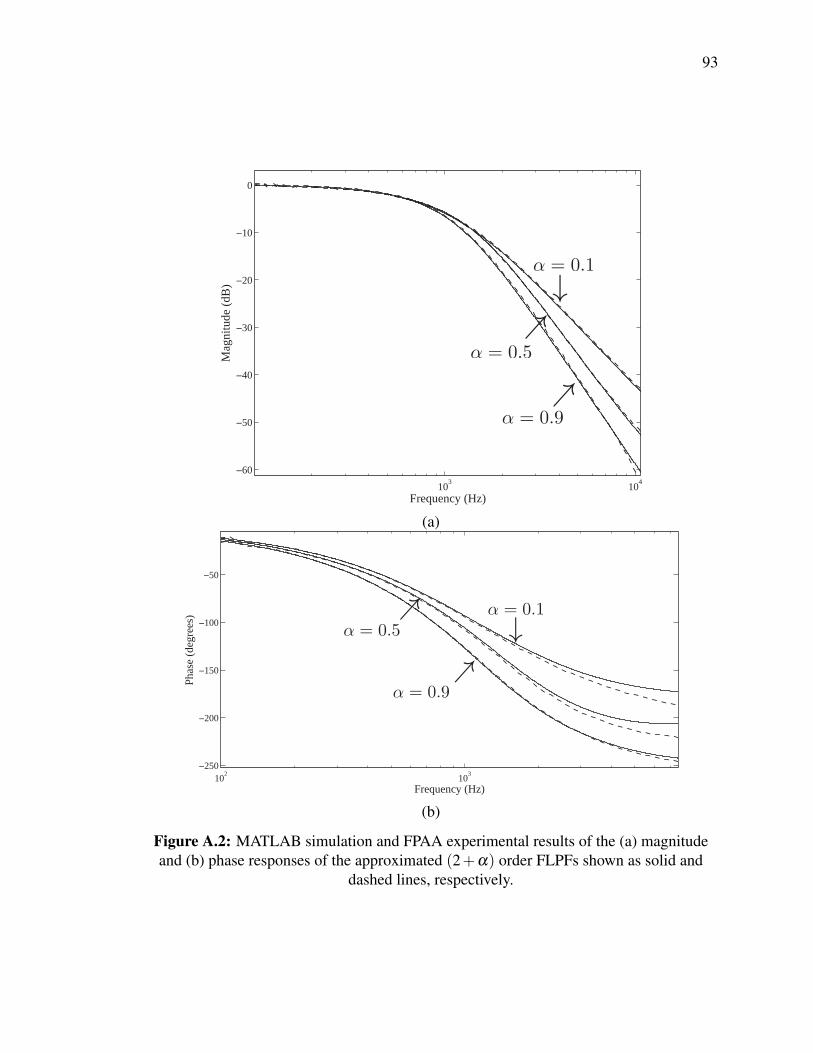
93

103

104

−60

−50

−40

−30

−20

−10

0

Frequency (Hz)

Mag

nit

ude

(dB

)

(a)

102

103

−250

−200

−150

−100

−50

Frequency (Hz)

Ph

ase

(deg

rees

)

(b)



94

103

104

−70

−60

−50

−40

−30

−20

−10

0

Frequency (Hz)

Mag

nit

ud

e (d

B)

(a)

102

103

−300

−250

−200

−150

−100

−50

Frequency (Hz)

Ph

ase

(deg

rees

)

(b)



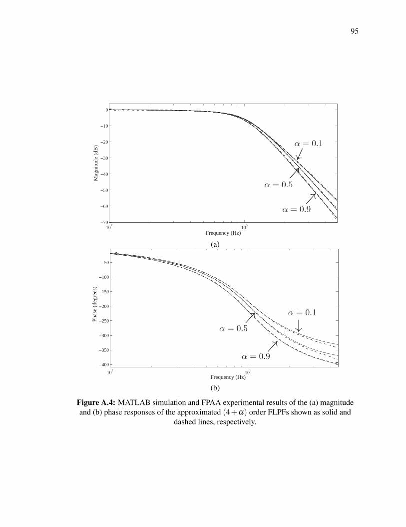
95

102

103

−70

−60

−50

−40

−30

−20

−10

0

Frequency (Hz)

Mag

nit

ud

e (d

B)

(a)

102

103

−400

−350

−300

−250

−200

−150

−100

−50

Frequency (Hz)

Ph

ase (

deg

rees)

(b)



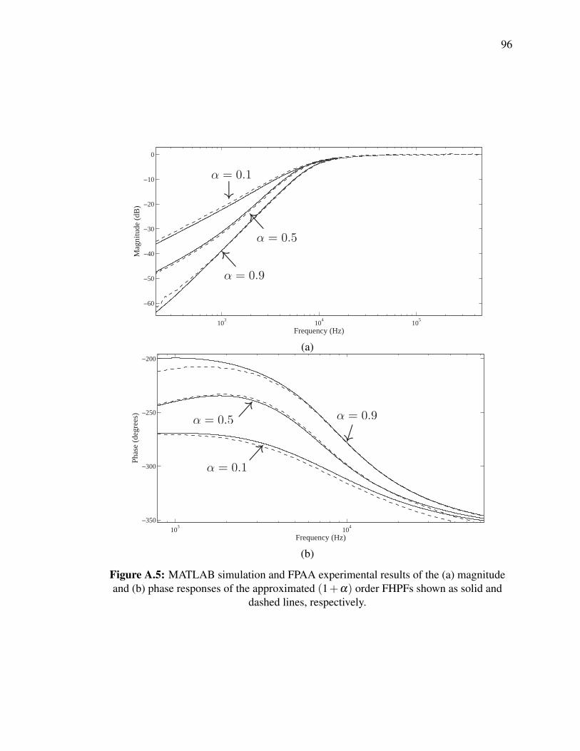
96

103

104

105

−60

−50

−40

−30

−20

−10

0

Frequency (Hz)

Mag

nit

ud

e (d

B)

(a)

103

104

−350

−300

−250

−200

Frequency (Hz)

Ph

ase

(deg

rees

)

(b)

Figure A.5: MATLAB simulation and FPAA experimental results of the (a) magnitudeand (b) phase responses of the approximated (1+a) order FHPFs shown as solid and


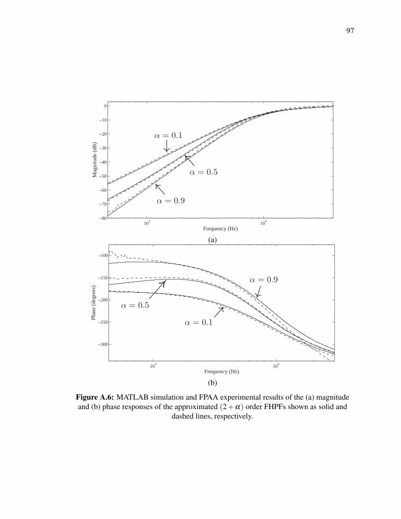
97

103

104

−80

−70

−60

−50

−40

−30

−20

−10

0

Frequency (Hz)

Mag

nit

ud

e (d

B)

(a)

103

104

−300

−250

−200

−150

−100

Frequency (Hz)

Ph

ase

(deg

rees

)

(b)



98

104

−60

−50

−40

−30

−20

−10

0

Frequency (Hz)

Mag

nit

ud

e (d

B)

(a)

103

104

−300

−250

−200

−150

−100

−50

Frequency (Hz)

Ph

ase

(deg

rees

)

(b)



99

104

−70

−60

−50

−40

−30

−20

−10

0

Frequency (Hz)

Mag

nit

ud

e (d

B)

(a)

104−300−250−200−150−100−50

050

Frequency (Hz)

Ph

ase

(deg

rees

)

(b)



APPENDIX B

REALIZATION OF AN APPROXIMATED FRACTIONAL CAPACITOR

Before we could simulate the approximated fractional Tow-Thomas biquad of Fig. 5.5,

an approximated fractional capacitor must be built. A realization using Carlson’s method

[29] was selected to model the fractional capacitors. Using this method approximations

of the general fractional capacitor, (1/s)1/n for n > 1, are possible. The order of these

approximations increasing as the number of iterations in the Newton process increases.

The function used in the regular Newton process for these approximations is

F(x) = x · (n�1)xn +(n+1)(1/s)(n+1)xn +(n�1)(1/s)

(B.1)

where x is the previous iteration. Using this process to approximate a fractional capacitor

when n = 2, or a = 0.5, using an initial assumption x0 = 1 yields

x1 =s+33s+1

(B.2)

as the first iteration approximatingp

1/s. The second iterate approximatingp

1/s is

x2 =s4 +36s3 +126s2 +84s+99s4 +84s3 +126s2 +36s+1

(B.3)

The magnitude response of this approximation is given in Fig. B.1. Note that this creates

an approximation of the fractional capacitor centered around the frequency 1rad/s. Using

the approximation of (B.3), the fractional Laplacian operator can be physically realized

101

10−2

10−1

100

101

102

−20

−15

−10

−5

0

5

10

15

20

Frequency (rad/s)

Mag

nit

ud

e (d

B)

Figure B.1: Magnitude response of the approximated fractional capacitor (dashed)compared to the ideal fractional capacitor of impedance Z(s) = 1/s0.5.

Figure B.2: RC ladder network to realize 4th order approximated fractional Laplacianoperator.

using the RC ladder network in Fig. B.2. The impedance of this RC ladder network is

Zin = Ra +1/Cb

s+ 1RbCb

+1/Cc

s+ 1RcCc

+1/Cd

s+ 1RdCd

+1/Ce

s+ 1ReCe

(B.4)

The resistor and capacitor values for the RC ladder in Fig. B.2 can be determined

102

through equating terms of (B.3) after a CFE of (B.4), which after the CFE becomes

1s0.5 ⇡ 1

9+

0.2291313787s+0.03109120413

+0.2962962975

s+0.3333333333+

1.899696037s+7.548632170

+0.5378392488

s+1.420276625(B.5)

We can approximate a fractional capacitor with any desired capacitance, C, centered around

any frequency, wc, by applying magnitude and frequency scaling factors to the component

values in the ladder realization. The resistor and capacitor values become

Rs = R · km (B.6)

Cs =C

k f km(B.7)

where Rs and Cs are the scaled resistor and capacitor values, R and C are the unscaled

resistor and capacitor values, km = 1Cw(1/n)

cis the magnitude scaling factor and k f = wc is the

frequency scaling factor. The magnitude response of the approximated fractional capacitor

after applying the scalings when C = 6.8nF and wc = 1000rad/s is shown in Fig. B.3.

The code used to generate the resistor and capacitor values for a fractional capacitor with

capacitance of 6.8nF , centre frequency of wc = 500rad/s, and n = 2 from (B.3) in MAPLE

is given in Fig. B.4.

103

101

102

103

104

105

110

115

120

125

130

135

140

145

150

155

X: 1000Y: 133.3

Frequency (rad/s)

Mag

nit

ude

(dB

)

Figure B.3: Magnitude response of the approximated fractional capacitor (dashed)compared to the ideal fractional capacitor of impedance Z(s) = 1/Cs0.5 after applying the

scalings when C = 6.8nF and wc = 1000rad/s.

104

Figure B.4: MAPLE code to calculate resistor and capacitor values for the ladderrealization of a fractional capacitor, Z(s) = 1/Cs0.5, of 6.8nF at a centre frequency of

500Hz.

design and implementation of fractional step filters

Documents