design and implementation of pv-firming and optimization
TRANSCRIPT

University of Central Florida University of Central Florida
STARS STARS
Electronic Theses and Dissertations, 2004-2019
2018
Design and Implementation of PV-Firming and Optimization Design and Implementation of PV-Firming and Optimization
Algorithms For Three-Port Microinverters Algorithms For Three-Port Microinverters
Mahmood Alharbi University of Central Florida
Part of the Power and Energy Commons
Find similar works at: https://stars.library.ucf.edu/etd
University of Central Florida Libraries http://library.ucf.edu
This Doctoral Dissertation (Open Access) is brought to you for free and open access by STARS. It has been accepted
for inclusion in Electronic Theses and Dissertations, 2004-2019 by an authorized administrator of STARS. For more
information, please contact [email protected].
STARS Citation STARS Citation Alharbi, Mahmood, "Design and Implementation of PV-Firming and Optimization Algorithms For Three-Port Microinverters" (2018). Electronic Theses and Dissertations, 2004-2019. 6237. https://stars.library.ucf.edu/etd/6237

DESIGN AND IMPLEMENTATION OF PV-FIRMING AND OPTIMIZATION
ALGORITHMS FOR THREE-PORT MICROINVERTERS
by
MAHMOOD ALI M ALHARBI
B.S. Taibah University, 2010
M.S. University of Colorado Colorado Springs, 2014
A dissertation submitted in partial fulfillment of the requirements
for the degree of Doctor of Philosophy
in the Department of Electrical & Computer Engineering
in the College of Engineering and Computer Science
at the University of Central Florida
Orlando, Florida
Fall Term
2018
Major Professor: Issa Batarseh

ii
© 2018 Mahmood Ali M Alharbi
iii
ABSTRACT
With the demand increase for electricity, the ever-increasing awareness of environmental issues,
coupled with rolling blackouts, the role of renewable energy generation is increasing along with
the thirst for electricity and awareness of environmental issues. This dissertation proposes the
design and implementation of PV-firming and optimization algorithms for three-port
microinverters.
Novel strategies are proposed in Chapters 3 and 4 for harvesting stable solar power in spite of
intermittent solar irradiance. PV firming is implemented using a panel-level three-port grid-tied
PV microinverter system instead of the traditional high-power energy storage and management
system at the utility scale. The microinverter system consists of a flyback converter and an H-
bridge inverter/rectifier, with a battery connected to the DC-link. The key to these strategies lies
in using static and dynamic algorithms to generate a smooth PV reference power. The outcomes
are applied to various control methods to charge/discharge the battery so that a stable power
generation profile is obtained. In addition, frequency-based optimization for the inverter stage is
presented.
One of the design parameters of grid-tied single-phase H-bridge sinusoidal pulse-width modulation
(SPWM) microinverters is switching frequency. The selection of the switching frequency is a
tradeoff between improving the power quality by reducing the total harmonic distortion (THD),
and improving the efficiency by reducing the switching loss. In Chapter 5, two algorithms are
proposed for optimizing both the power quality and the efficiency of the microinverter. They do

iv
this by using a frequency tracking technique that requires no hardware modification. The first
algorithm tracks the optimal switching frequency for maximum efficiency at a given THD value.
The second maximizes the power quality of the H-bridge micro-inverter by tracking the switching
frequency that corresponds to the minimum THD.
Real-time PV intermittency and usable capacity data were evaluated and then further analyzed in
MATLAB/SIMULINK to validate the PV firming control. The proposed PV firming and
optimization algorithms were experimentally verified, and the results evaluated. Finally, Chapter
6 provides a summary of key conclusions and future work to optimize the presented topology and
algorithms.

v
To My Parents
Safiah & Ali

vi
ACKNOWLEDGMENT
I would like to express my sincere gratitude and appreciation to the government of the Kingdom
of Saudi Arabia, Ministry of Education in Saudi Arabia, and Taibah University for their financial
support and continuous motivation to my study for the PhD at the University of Central Florida.
They have provided all means to create an appropriate learning environment.
I would like to express my sincere appreciation and gratitude to Professor Issa Batarseh, my
academic advisor, for his patient guidance, enthusiastic encouragement and useful critiques of this
research work throughout my studies and research at University of Central Florida. His guidance
helped me in all the time of research and writing of this dissertation. Beside his support and
immense knowledge, he has always given me great chances to pursuit my work independently.
Besides my advisor, I would like to thank the rest of my thesis committee: Dr. Nasser Kutkut, Dr.
Wasfy B. Mikhael, Dr. Michael Haralambous and Dr. Jiann S. Yuan, for their insightful comments
and encouragement.
I would like to thank the team members in the Florida Power Electronics Center (FPEC), and
special thanks to Dr. Haibing Hu, Siddhesh Shinde, and Anirudh Pise for their invaluable support
and time spent on my research.
I would like to thank the team members in the Florida Solar Energy Center (FSEC) for providing
me with invaluable real-time data for the PV intermittency.

vii
I would like to thank the team members in the Advanced Power Electronics Corporation
(ApECOR), and special thanks to Chris Hamilton and Michael Pepper for helping me performing
the algorithms coding.
I would like to thank the team members in the Advanced Charging Technology (ACT) Engineering
Center in Orlando, FL, and special thanks to Dr. Nasser Kutkut and Charles Jourdan for helping me
constructing the hardware.
I would like to express my appreciation to Dr. Ala Hussein from Yarmouk University for his
guidance and support.
Finally, I would like to thank my parents, Safiah and Ali, and my wife Razan Alahmadi, for
supporting me spiritually throughout my study and my life in general.
viii
TABLE OF CONTENTS
LIST OF FIGURES ....................................................................................................................... xi
LIST OF TABLES ....................................................................................................................... xvi
CHAPTER 1: INTRODUCTION ................................................................................................... 1
1.1 Background ...................................................................................................................... 1
1.1.1 The Nature of PV Energy ......................................................................................... 1
1.1.2 Weather Instability Effects on PV Power ................................................................. 5
1.1.3 Ramp-Rate and Ramping Frequency of PV Output ................................................. 7
1.1.4 Energy Storage Technology .................................................................................... 12
1.1.5 Integration of PV and Energy Storage .................................................................... 16
1.2 Research Motivation and Objective ............................................................................... 19
CHAPTER 2: LITERATURE REVIEW ...................................................................................... 21
2.1 PV Firming Technologies .............................................................................................. 21
2.2 Three-Port PV Connected Microinverters...................................................................... 26
2.3 Merits Comparison between Reviewed and Proposed Technologies ............................ 33
CHAPTER 3: PROPOSED TOPOLOGY AND STATIC PV FIRMING ALGORITHM .......... 36
3.1 Introduction .................................................................................................................... 36
3.2 Proposed Topology and Operational Principle .............................................................. 37
3.2.1 The Topology .......................................................................................................... 37

ix
3.2.2 Implemented Controls Regardless of the Proposed Algorithms ............................. 39
3.3 Proposed Static PV Firming Algorithm ......................................................................... 45
3.3.1 Static PV Reference Generation Method ................................................................ 45
3.3.2 Battery Charging/ Discharging Algorithm.............................................................. 49
3.4 Simulation Results.......................................................................................................... 54
3.5 Experimental Results...................................................................................................... 56
3.6 Storage Capacity Sizing Analysis for the Static PV Reference ..................................... 61
3.7 Conclusions .................................................................................................................... 68
CHAPTER 4: DYNAMIC PV FIRMING ALGORITHM ........................................................... 69
4.1 Introduction .................................................................................................................... 69
4.2 Proposed Dynamic PV Firming System......................................................................... 69
4.2.1 Dynamic PV Reference Generation Algorithm ...................................................... 69
4.2.2 Battery Charging/ Discharging Algorithm.............................................................. 77
4.3 Simulation Results.......................................................................................................... 78
4.4 Experimental Results...................................................................................................... 80
4.5 Storage Capacity Sizing Analysis for the Dynamic PV Reference ................................ 84
4.6 Conclusions .................................................................................................................... 90
CHAPTER 5: DUAL OPTIMIZATION FOR THE INVERTION STAGE ................................ 92
5.1 Introduction .................................................................................................................... 92
x
5.2 Loss Modeling and Calculation...................................................................................... 93
5.3 Optimal Switching Frequency Tracking Algorithms ..................................................... 98
5.3.1 THD and Efficiency ................................................................................................ 99
5.3.2 Approach 1: Dual Tracking of Optimum Efficiency and THD Algorithm .......... 101
5.3.3 Approach 2; Minimum THD Point Tracking Algorithm ...................................... 104
5.4 Experimental Results.................................................................................................... 106
5.5 Conclusions .................................................................................................................. 110
CHAPTER 6: SUMMARY AND FUTUTRE WORKS ............................................................ 112
6.1 Summary ...................................................................................................................... 112
6.2 Future Works ................................................................................................................ 116
APPENDIX A: FSEC DATA SOURCE .................................................................................... 118
A.1 What is FSEC? ................................................................................................................. 119
A.2 Data Collected for Modular PV System .......................................................................... 119
A.3 Case Study-Data from FSEC ........................................................................................... 120
APPENDIX B: PV ENERGY PLOTS FOR TWELVE MONTHS ........................................... 122
APPENDIX C: EQUATIONS OF THE INVERTER POWER LOSSES .................................. 129
LIST OF REFERENCES ............................................................................................................ 133

xi
LIST OF FIGURES
Figure 1: Map of photovoltaics and concentrating solar power source potential for the United
States[1]. ......................................................................................................................................... 2
Figure 2: Actual and ideal PV power. ............................................................................................. 3
Figure 3: Measured PV power profiles (blue curves) for each day in April 2016 (x-axis: Time
(minute), y-axis: Powe (Watt)). ...................................................................................................... 4
Figure 4: Average, maximum, and minimum PV capacity in Watt-hour based on real-time data in
East Florida (Appendix A). ............................................................................................................. 5
Figure 5: Summery for undesirable effects of the PV variability. .................................................. 6
Figure 6: Ramping frequency 60W (10% nominal power) in different time scales for two different
days. ................................................................................................................................................ 8
Figure 7: Time of ramp-rate higher than 10%/min. of the rated PV power (600W) for each day in
April 2016. .................................................................................................................................... 10
Figure 8: Average daily ramp-rate higher than 10%/min. of 600W rated PV output power for each
month from Feb. 2016 to Jan. 2017. ............................................................................................. 11
Figure 9: Architectures of PV and energy storage integration; (a) DC-side battery connection via
DC/DC stage, (b) AC-side battery connection via DC/AC stage, (c) PV-battery integrated three-
port DC/DC converter, and (d) DC-link battery direct connection. ............................................. 18
Figure 10: Grid-tied PV firming system[36]. ............................................................................... 22
Figure 11: PV-EDLC system for controlling the PV output ramp-rate [40]. ............................... 22
Figure 12: PHEV bidirectional battery charger integrated to a PV system [37] .......................... 24
Figure 13: Interleaved boost convert based topology [52], [53] ................................................... 27

xii
Figure 14: A stand-alone PV/battery system proposed by [54]. ................................................... 28
Figure 15: A multiport AC link PV inverter with reduced size and weight for stand-alone
application by [55] ........................................................................................................................ 30
Figure 16: A single-stage microinverter without using electrolytic capacitors by [56]. .............. 31
Figure 17: A soft-switched three-port single-phase microinverter topology by [58]. .................. 32
Figure 18: The proposed grid-tie three-port PV microinverter. .................................................... 38
Figure 19: Block diagram for the proposed three-port system with the implemented controls
without firming algorithms. .......................................................................................................... 39
Figure 20: Perturbation and observation (P&O) algorithm. ......................................................... 40
Figure 21: Block diagram of the used PLL controller. ................................................................. 41
Figure 22: Block diagram for the DC-link voltage regulation control (DCVR). .......................... 43
Figure 23: Block diagram for the output current regulation control (OCR). ................................ 44
Figure 24: Maximum and average PV reference power compared to PV actual power on different
days in 2016, where (a) is on Feb, 19th, (b) is on May, 14th, and (c) is on Aug, 17th. ................... 48
Figure 25: Architecture of the proposed PV firming system. ....................................................... 50
Figure 26: The algorithm flowchart for the PV firming battery charge/discharge control. .......... 50
Figure 27: Scenarios configuration for the inverter reference current generation. ....................... 53
Figure 28: Power waveforms for PV reference (scatter black), PV actual (blue), firmed inverter
output (red), and battery (green) for the static firming microsystem. ........................................... 55
Figure 29: DC-link voltage (Vdc-link), inverter output current (Iinv), and inverter reference RMS
current (Iinv,ref) waveforms. ........................................................................................................ 56

xiii
Figure 30: Power waveforms for PV actual, inverter output (firmed), and battery for static firming.
....................................................................................................................................................... 59
Figure 31: Grid voltage (Vg), DC-link voltage (Vdc-link), inverter output current (Iinv), and battery
current (Ibat) waveforms while the battery is being charged. ........................................................ 60
Figure 32: Grid voltage (Vg), DC-link voltage (Vdc-link), inverter output current (Iinv), and battery
current (Ibat) waveforms while the battery is being discharged. ................................................... 61
Figure 33: Average, maximum, and minimum PV energy for month of (a) Feb. 2016 and (b) Jun.
2016............................................................................................................................................... 65
Figure 34: Analysis of PV and average storage capacities when the system is assumed to be firmed
statically. ....................................................................................................................................... 67
Figure 35: The maximum PV reference power with generated power levels............................... 72
Figure 36: Proposed algorithm for dynamic PV reference power generation. ............................. 73
Figure 37: Generated PV firming reference for two different days. ............................................. 76
Figure 38: The algorithm flowchart for the PV firming battery charge/discharge control ........... 78
Figure 39: Power waveforms for PV actual (blue), firmed inverter output (red), and battery (green)
for the dynamic firming microsystem. .......................................................................................... 79
Figure 40: DC-link voltage (Vdc-link), inverter output current (Iinv), and inverter reference RMS
current (Iinv,ref) waveforms. ........................................................................................................ 80
Figure 41: Power waveforms for PV actual, inverter output (firmed), and battery for static firming.
....................................................................................................................................................... 82
Figure 42: Grid voltage (Vg), DC-link voltage (Vdc-link), inverter output current (Iinv), and battery
current (Ibat) waveforms while the battery is being charged. ........................................................ 83
xiv
Figure 43: Grid voltage (Vg), DC-link voltage (Vdc-link), inverter output current (Iinv), and battery
current (Ibat) waveforms while the battery is being discharged. ................................................... 84
Figure 44: Power waveforms of PV actual (blue), PV reference/ firmed inverter output (red), and
battery (orange), such an example for a day in May 2016. ........................................................... 85
Figure 45: Analysis of PV and usable storage capacities when the system is firmed dynamically.
....................................................................................................................................................... 87
Figure 46: Power waveforms for same example shown in Figure 44 but with different fluctuation
factor (ls=0.1). ............................................................................................................................... 89
Figure 47: Power waveforms for same example shown in Figure 28 but with different fluctuation
factor (ls=0.3)). ............................................................................................................................. 90
Figure 48: H-bridge microinverter topology................................................................................. 94
Figure 49: (a) Modes of operation waveforms. (b) Modes of operation circuits diagram. ........... 96
Figure 50: Power losses in percentage for the microinverter when the switching frequency is
20kHz. ........................................................................................................................................... 98
Figure 51: Proposed algorithm for dual tracking of optimum efficiency and THD values for the H-
bridge SPWM inverter (Approach 1). ......................................................................................... 102
Figure 52: Switching frequency zones and optimum THD point. .............................................. 103
Figure 53: Minimum THD point tracking algorithm (Approach 2). .......................................... 105
Figure 54: Efficiency versus switching frequency at different loads. ........................................ 107
Figure 55: THD versus switching frequency at different loads. ................................................. 108
Figure 56: Optimum switching frequencies for maximum efficiency and THD below 4%
(Approach 1). .............................................................................................................................. 109

xv
Figure 57: Optimum switching frequencies for highest power quality at minimum THD (Approach
2). ................................................................................................................................................ 110

xvi
LIST OF TABLES
Table 1: Technical Characteristics for Different Energy Storage Technologies .......................... 15
Table 2: Summary for a comparison between different PV-firming technologies. ...................... 25
Table 3: Key characteristics of presented topologies ................................................................... 33
Table 4: Merits comparison between PV-firming technologies. .................................................. 35
Table 5: Prototype specifications .................................................................................................. 57
Table 6: Technical Specifications of the Battery Used in the Experiment. .................................. 58

1
CHAPTER 1: INTRODUCTION
1.1 Background
1.1.1 The Nature of PV Energy
The nature of the photovoltaic (PV) energy is based on two factors; the nature of the sunlight
(irradiance) and temperature. These two factors depend on the location on the earth. For example,
the concentrating solar power resource potential for the United States changes in each state as
shown in Figure 1, [1]. In Colorado for instance, the annual average solar resource changes from
about 4.5 to 6.5 kWh/m2/Day. Additionally, due to weather changes such as cloud passing, the
PVs deliver power intermittently although the ideal shape of the PV output power is a parabolic
curve. Figure 2 illustrates an example of the actual PV power and the ideal PV power measured
for one-minute time resolution. The x-axis in the figure represents the time in minutes, where it
begins from minute 1 (at midnight, 00:00) to minute 1440 (just before midnight, 23:59). The y-
axis represents the power in watt (W), where the maximum power delivered by the PV is about
600W. The fluctuations shown in the actual PV power indicates the times of cloud passing.
Similarly, this variation occurs every day. Figure 3 shows an example of the PV out power
variations throughout the month of April 2016. These curves are based on real-time data collected
for PV intermittency from two 300W PV modular systems including PV panels and a grid-tied
microinverter located in a specific region in East Florida [2]. More information about the data

2
collected is given in Appendix A and B. Moreover, the average, maximum, and minimum PV
capacities (Wh) change every month as shown in Figure 4. That concludes that this instability
supports the need for energy storage which is the only facility that we can use for this challenge.
Figure 1: Map of photovoltaics and concentrating solar power source potential for the United
States[1].

3
Figure 2: Actual and ideal PV power.

4
Figure 3: Measured PV power profiles (blue curves) for each day in April 2016 (x-axis: Time
(minute), y-axis: Powe (Watt)).

5
Figure 4: Average, maximum, and minimum PV capacity in Watt-hour based on real-time data in
East Florida (Appendix A).
1.1.2 Weather Instability Effects on PV Power
Solar PV power generation is highly unstable due to the irregular changes in the sun irradiance
level caused by weather changes and passing clouds. In large utility and auxiliary fuel power
generators, the time response can be as long as tens of seconds or more. This is insufficient to
compensate for those renewable sources with high variability such as the PV. Cloud passing effects
on the PV have been studied for a long time [3], [4], [5], [6], [7]. Some studies address this problem
as a contemporaneous issue [8] [9], and focus on the high penetration level of PV generation.
Several undesirable effects of the PV variability are voltage fluctuations at the distribution system

6
level, and frequency instability in small grids. The voltage fluctuations can lead to voltage flicker
and excessive Load Tap Changer (LTC) operation. In small grids, the frequency instability can
lead to increased damage to conventional voltage regulator equipment. These effects provide more
challenges to higher penetration of PV in general and at the distribution levels particularly. Figure
5 summarizes these effects in flowchart.
Figure 5: Summery for undesirable effects of the PV variability.
7
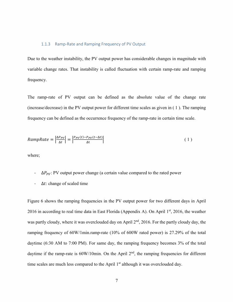
1.1.3 Ramp-Rate and Ramping Frequency of PV Output
Due to the weather instability, the PV output power has considerable changes in magnitude with
variable change rates. That instability is called fluctuation with certain ramp-rate and ramping
frequency.
The ramp-rate of PV output can be defined as the absolute value of the change rate
(increase/decrease) in the PV output power for different time scales as given in ( 1 ). The ramping
frequency can be defined as the occurrence frequency of the ramp-rate in certain time scale.
𝑅𝑎𝑚𝑝𝑅𝑎𝑡𝑒 = |Δ𝑃𝑃𝑉
Δ𝑡| = |
𝑃𝑃𝑉(𝑡)−𝑃𝑃𝑉(𝑡−Δ𝑡)
Δt| ( 1 )
where;
- Δ𝑃𝑃𝑉: PV output power change (a certain value compared to the rated power
- Δ𝑡: change of scaled time
Figure 6 shows the ramping frequencies in the PV output power for two different days in April
2016 in according to real time data in East Florida (Appendix A). On April 1st, 2016, the weather
was partly cloudy, where it was overclouded day on April 2nd, 2016. For the partly cloudy day, the
ramping frequency of 60W/1min.ramp-rate (10% of 600W rated power) is 27.29% of the total
daytime (6:30 AM to 7:00 PM). For same day, the ramping frequency becomes 3% of the total
daytime if the ramp-rate is 60W/10min. On the April 2nd, the ramping frequencies for different
time scales are much less compared to the April 1st although it was overclouded day.

8
Figure 6: Ramping frequency 60W (10% nominal power) in different time scales for two
different days.

9
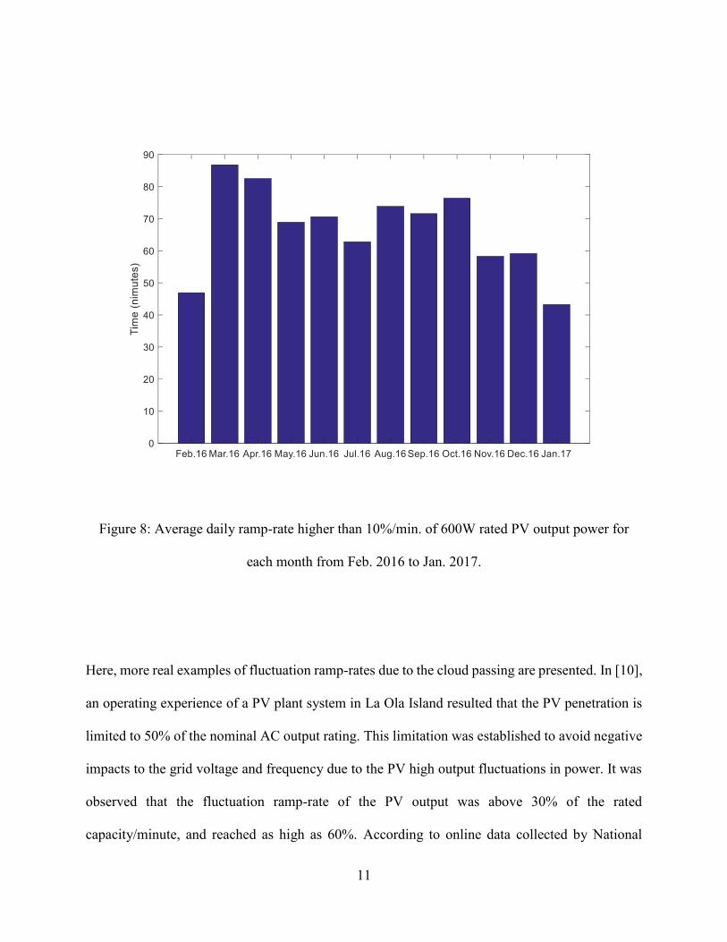
Figure 7 shows the daily time (in minute) of ramp-rate higher than 10%/min. of 600W rated PV
output power in April 2016. Noticeably, the time of over limited ramp-rate varies from 0 minute
up to more than 3 hours. Also, this variability can be explained by analyzing the average daily
ramp-rate higher than the limit, where the limit here is considered to be 10%/min of the 600W
rated PV output power. This average can be determined for the whole year. Figure 8 shows the
average daily high ramp-rate (more than 10%/min.) for each month from February 2016 to January
2017 according to same data collected by [2] (Appendix A).

10
Figure 7: Time of ramp-rate higher than 10%/min. of the rated PV power (600W) for each day in
April 2016.
11
Figure 8: Average daily ramp-rate higher than 10%/min. of 600W rated PV output power for
each month from Feb. 2016 to Jan. 2017.
Here, more real examples of fluctuation ramp-rates due to the cloud passing are presented. In [10],
an operating experience of a PV plant system in La Ola Island resulted that the PV penetration is
limited to 50% of the nominal AC output rating. This limitation was established to avoid negative
impacts to the grid voltage and frequency due to the PV high output fluctuations in power. It was
observed that the fluctuation ramp-rate of the PV output was above 30% of the rated
capacity/minute, and reached as high as 60%. According to online data collected by National

12
Renewable Energy Lab (NREL) [11] from Oahu Island, the irradiance fluctuations can have more
than 50% ramp-rate in two consecutive measurements. In a study presented in Mesa del Sol, New
Mexico [12], PV output was found to ramp up more that ±30% of normal operating power by rated
capacity per second. A technical report presented by the Commonwealth Scientific and Industrial
Research Organization (CSIRO) [13] in Newcastle, Australia has shown that over 31% ramp-rate
of the plant rating can occurs up to 120 time in 10 seconds. These and other documented examples
demonstrate that the high ramp-rate fluctuations of the PV output can produce considerable voltage
variations that need to be managed [14].
PV-firming strategies and algorithms that control ramp-rate to reduce fluctuations in PV outputs
are necessary to increase the PV penetration level in networks. Energy storage is the most practical
tool to be used to achieve this goal. Since all energy storage devices absorb and deliver DC power,
they rely on power electronics systems, like any renewable energy sources, for interfacing with
the AC grid. So, novel approaches and algorithms for a PV-firming system integrating an energy
storage as a third port is presented in this dissertation.
1.1.4 Energy Storage Technology
Solar and wind are two different sources of renewable energy that delivers high intermittent
powers. Generally, these renewables energies are unreliable and often applied concurrently with
electrical energy storage systems to enhance their reliability in the network [15]. This enhancement

13
is by reducing the power fluctuations, improving the power quality, and enhancing the system
flexibility.
There are four categories of energy storage technologies mostly used in electric power systems:
chemical, electrochemical, electromagnetic, and mechanical [16], [17], [18], [19], [20]. Each
technology has distinctive specifications in terms of different characteristics that are taken into
account for comparison. These characteristics are energy density, power capacity, discharge time,
life and cycling time, response time, and discharge efficiency.
1.1.4.1 Chemical Energy Storage
There are two types of chemical energy storage technology: synthetic natural gas (SNG) energy
storage and hydrogen (H2) energy storage [21]. For the H2 energy storage technology, H2 is
extracted from the water (H2O) by decomposition process with electricity. Then, it is stored in
high-pressure tanks and delivered to a fuel cell for ionizing and producing electricity. The main
advantage of this technology is its capability of long period storage [22]. However, the main
drawback is its high cost due to the expense of producing the H2 and manufacturing the fuel cells.
For the other technology of SNG energy storage, the pressure of the SNG tank is lower than the
H2 tank since the SNG has higher density. However, its conversion losses are higher than H2’s
[21].
14
1.1.4.2 Electrochemical Energy Storage
The most common definition for the electrochemical energy storage is battery. There are three
main types of battery: lead acid (LA), lithium ion (Li-ion), and vanadium redox battery (VRB).
The LA battery is a traditional battery that is widely applied in several applications because of its
low costs. However, it has limited life and cycling times, low energy density, and low efficiency
[19]. One the contrary, the Li-ion battery has higher life and cycling times, higher energy density,
and higher efficiency [17]. As a disadvantage of the Li-ion battery, its cost is still high comparing
to the LA battery. The VRB has also high life and cycling times, but its efficiency decreases in the
cold temperature.
1.1.4.3 Electromagnetic Energy Storage
In this technology, the energy is stored in either electric fields (supercapacitor (SC) energy storage
device) or magnetic fields (superinducting magnetic energy storage (SMES)) [23], [24]. Both
technologies have very low energy density that makes them unsuitable for long discharging time
applications.
1.1.4.4 Mechanical Energy Storage
When there is surplus power during off-peak time, the electricity is transferred mechanically to a
mechanical storage system. The energy can be stored for long time, and it is released once needed.

15
The energy is stored in the form of gravitational potential energy (pumped hydroelectric energy
storage (PHES)), intermolecular potential energy (compressed air energy storage (CAES)), or
rotational energy (flywheel energy storage (FES)) [25], [26]. PHES and CAES technologies have
very high power capacity cycling times. However, their response time is slow comparatively.
Table 1 summarizes comparison of the energy storage technologies in terms of energy density,
power capacity, discharge time, life time, cycling time, response time, and discharge efficiency
[16], [17], [18], [19], [20], [23], [24], [25], [26], [22], [21], [27].
Table 1: Technical Characteristics for Different Energy Storage Technologies
Energy Power Discharge Life Cycling Response Discharge
Density Capacity Time Time Time Time Efficiency
(Wh/L) (W) (years) (cycles) (%)
SNG 800 − 5000 1M − 100 M hours 15 ~20000 seconds ~50
H2 500 − 3000 450k − 45M hours 15 ~10000 seconds ~59
LA 50 − 90 1k − 10M minutes 3 ~1000 milliseconds ~85
Li-ion 200 − 500 1k − 70k minutes 5 − 10 ~5000 milliseconds ~85
VRB 12 − 22 450k − 45M hours 5 − 15 ~10000 milliseconds ~85
SC 10 − 30 10k − 400k seconds 10 − 30 ~50000 milliseconds ~95
SMES 1 − 7 1M − 10M seconds >20 ~100000 milliseconds ~95
PHES 1 − 2 250M − 950M hours 40 − 60 ~30000 minutes ~87
CAES 2 − 5 100M − 980M hours 20 − 40 ~10000 minutes ~75
FES 20 − 80 1k − 75k minutes 15 ~20000 seconds ~90
Chemical
Electrochemical
Electromagnetic
Mechanical

16
1.1.5 Integration of PV and Energy Storage
Many researches have proposed different power electronics topologies for integrating PV and
energy storage systems. Each topology must be under one of main four architectures as shown in
Figure 9, where the energy storage is considered as a battery and the power flow described by blue
arrows. Since all architectures are grid-tied, it must have at least one inversion (DC/AC) stage. In
the first architecture shown in Figure 9 (a), both PV and battery are connected throughout a
separate DC/DC stage to the DC side of the DC/AC stage. Second architecture shown in Figure 9
(b) connects the battery to the AC side through another DC/AC stage. Third architecture shown in
Figure 9 (c) integrates both PV and battery throughout a three-port DC/DC converter, where the
third port is connected to the DC side of the DC/AC stage. Last architecture shown in Figure 9 (d)
eliminates one DC/DC stage by connecting the battery to the DC-link directly.

17
(a)
(b)

18
(c)
(d)
Figure 9: Architectures of PV and energy storage integration; (a) DC-side battery connection via
DC/DC stage, (b) AC-side battery connection via DC/AC stage, (c) PV-battery integrated three-
port DC/DC converter, and (d) DC-link battery direct connection.

19
1.2 Research Motivation and Objective
In recent decades, several researches have paid more attention considerably on the renewable
energy worldwide, where electricity generation by photovoltaic (PV) is becoming one of the most
common clean and abundance energy sources. Although PV is becoming increasingly cost
effective, there are several technical challenges which limit its penetration into the grid. Distributed
energy storage seems to hold the key in unlocking the full potential of the renewable energy
resources. Recent studies have focused on battery storage at both utility and distributed scale.
Many advantages (e.g. energy arbitrage, increased PV self-consumption, transmission congestion
relief, VAR support etc.) of such storage across various players ranging from independent system
operators to end users are extensively reported in [28],[29],[30],[31],[32],[33], and [34]. As PV
penetration increases rapidly while distributed battery systems are expected to become ubiquitous
with falling prices [35], incentives lie in integrating batteries, PV panel and advanced power
electronics that may provide stable power profiles, and reduced system infrastructure complexity.
So, the objectives of this dissertation are to develop an integration of PV, battery, and power
electronics in one modular level system with the capability of PV-firming and energy management.
More specifically, the development targets for the integrated system are summarized as follows:
✓ To make an integration of PV, battery, and grid in one modular micro-system
✓ To minimize the number of conversion stages
✓ To employ the capability bidirectional power flow
✓ To implement smart functions such as: Grid support, maximum power tracking (MPPT)
for the PV

20
✓ To firm the PV output profile to increase its penetration level in the networks
With the above development targets, the research objectives of this dissertation can be summarized
as follows:
✓ To design and implement a smart integration of the battery into the grid-tied power
electronics without additional conversion stage
✓ To design and implement all different control methods that can be implemented fully using
the digital control, which increase both the power density and reliability and decrease the
cost of the micro-system
✓ To design and implement a control method that is used for battery charging and discharging
✓ To design and implement new algorithms that are used for firming the PV output profile
✓ To design and implement new algorithms that are used for optimizing both efficiency and
output power quality for the inversion stage of the micro-system
21
CHAPTER 2: LITERATURE REVIEW
2.1 PV Firming Technologies
Several types of technologies based on energy storage have been proposed for firming the PV
output power. Different kinds of storages have been used, such as: battery energy storage [36],[37];
fuel cell energy [38]; superconductive magnetic energy storage [39]; and electric double-layer
capacitor (EDLC) [40], [41].
Figure 10 shows , a high-power level system of grid-tied PV firming [36]. This system uses a valve
regulated lead-acid (VRLA) battery temporarily to charge and discharge as required for firming
the inverter output power. A moving average calculation was used to control the inverter output
power by averaging the solar irradiance over the previous one-hour time interval. A similar control
method was used in [40]. Here an EDLC is connected in parallel to the DC-link between the DC-
DC converter stage and the DC-AC inverter stage as shown in Figure 11.

22
Figure 10: Grid-tied PV firming system[36].
Figure 11: PV-EDLC system for controlling the PV output ramp-rate [40].
Another method to smooth the PV output power is by using a battery energy storage system
(BESS) as in [42]. Here a large-scale BESS system was interfacing with PV and wind power

23
systems through the grid. The firming control was based on storage capacity, where the charging/
discharging scenarios were according to the state of charge (SOC) of the batteries.
PV fluctuation ramp-rate can be assumed as rapid changings with different values of slope. These
changes can be compensated for to maintain a minimum value of slope as in [43]. An energy
storage has been deployed in this research. Although the control strategy was independent on the
previous PV intermittency history like the traditional moving average method, the calculation of
the slope that is based on the differentiation of the PV power over time makes delaying to the
results practically.
In [44] and [45], a medium voltage scale of BESS is used for PV capacity firming and shifting.
The algorithm for firming was based on the maximum and minimum power reference for the PV
output. Two bidirectional conversion systems were connected to the BESS for charging and
discharging through the grid.
Plug-in hybrid electric vehicle (PHEV) batteries have been utilized in [37] to mitigate the solar
irradiance intermittency at short time scales. Here a bidirectional DC-DC (buck-boost) charger is
integrated in the PV system as shown in Figure 12, where the communication point was the DC-
link. A high-pass filter was used for fluctuation mitigation. The corner frequency (filter
characteristic), was used to limit the ramp-rate of the PV inverter.

24
Figure 12: PHEV bidirectional battery charger integrated to a PV system [37]

25
A simulation study has been done by [38] that integrates a fuel cell to a PV grid-tied and stand-
alone system. The charging discharging method was simply to maintain the match between the
output power of the system and the load rate. Similarly, in [46], hydrogen energy has been used in
a PV system to balance the fluctuation of PV output power. An exponential moving average was
used for PV-firming.
Table 2 summarizes the differences between all reviewed PV-firming technologies in terms of
energy storage used in the system, the category of the PV-storage integration (Figure 9), firming
method applied in the control, and the rated power.
Table 2: Summary for a comparison between different PV-firming technologies.
PV-Firming Energy Integration Firming Rated
Technology Storage Category Method Power(W)
Ref. [36] VRLA AC-Side Moving Average 3.5 k
Ref. [37] PHEV Battery DC-Side Corner Freq. (Filter) 25 k
Ref. [38] Fuel Cell DC-Side Load-based 20 M
Ref. [39] SMES AC-Side Load-based 40 M
Ref. [40] EDLC DC-Link Moving Average 1 k
Ref. [41] EDLC DC-Side Moving Average 200 k
Ref. [42] BESS AC-Side Storage Capacity-based 1 M
Ref. [43] LA Battery DC-Side Power slope-based 400
Ref. [44],[45] BESS AC-Side Limits (max. & min.)-based 1 M
Ref. [46] Hydrogen DC-Side Exponential Moving Average 3 k

26
2.2 Three-Port PV Connected Microinverters
Recent, but limited, studies were found using three-port microinverter that integrates PV and
storage. Similar to the two-port microinverter, there are several advantages of the three-port micro-
conversion system over the utility scale system as follows as discussed in [47], [48], [49], [50],
and [51].
1) Independently Control Optimization: Every individual PV panel conversion system can
independently control and optimize the power flow in all directions. Every system can
independently and optimally charge and discharge its battery. For each PV, the converter
can independently obtain maximum power point tracking (MPPT).
2) Battery Management and Protection: Every battery can be replaced or fixed when it reaches
its maximum number of life cycles or needs maintenance. Battery protection can be applied
intelligently for each PV panel converter. In other word, based on the state of charge (SOC),
for instance, each battery can be protected from damage due to deep discharge.
3) Improved Data Collecting Capability: Every PV-battery-conversion module can have a
permanent data collection capability. There can be a control network connection between
all modules and converters. This can facilitate the maintenance requirement for each PV
panel or battery.
4) Improved Maintenance: If one of the devices doesn’t work properly, the system doesn’t
have to be shut down totally in order to replace or repair.
27
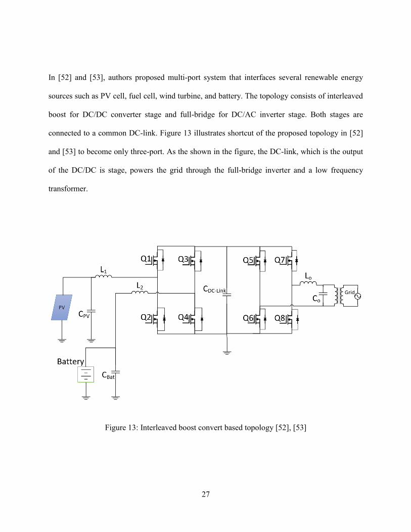
In [52] and [53], authors proposed multi-port system that interfaces several renewable energy
sources such as PV cell, fuel cell, wind turbine, and battery. The topology consists of interleaved
boost for DC/DC converter stage and full-bridge for DC/AC inverter stage. Both stages are
connected to a common DC-link. Figure 13 illustrates shortcut of the proposed topology in [52]
and [53] to become only three-port. As the shown in the figure, the DC-link, which is the output
of the DC/DC is stage, powers the grid through the full-bridge inverter and a low frequency
transformer.
Figure 13: Interleaved boost convert based topology [52], [53]

28
Figure 14 illustrates a three-port conversion system integrated with battery for PV stand-alone
applications presented by [54]. This topology is achieved based on a traditional half-bridge two-
port converter, where the middle devices of S3 and D3 are added to integrate a third port (battery)
conversion stage. MPPT control is applied at the PV port, while bidirectional charging/ discharging
control is implemented at the battery port. Hence, a rectified sinusoid voltage is generated. A low
frequency (50/ 60Hz) unfolding circuit is cascaded to perform sinusoid AC voltage.
Figure 14: A stand-alone PV/battery system proposed by [54].
Figure 15 displays a non-isolated single-stage three-port microinverter with high-frequency AC
link based interfacing [55]. It is multi-input/ multi-output and three-phase inversion topology with
power level of 800W. The bridges for battery and grid ports have bidirectional switches to enable
bidirectional conversions for charging and discharging the battery. The AC link consists of low
reactive parallel LC components which make partial resonance in the conversion system. The main

29
storage component in this topology is the inductor. The capacitor component helps the inductor
facilitate the partial resonance during the operation modes of power conversion. Zero voltage turn
on of the switches and higher efficiency are a result of the partial resonance. The difference
between this three-port microinverter and the resonant converters is the shortened resonance time.

30
Figure 15: A multiport AC link PV inverter with reduced size and weight for stand-alone
application by [55]
Another three-port microinverter has been presented in [56] and [57] in which the third port is
intended to achieve the power decoupling function. It is based on the three-port flyback topology,

31
as shown in Figure 16. It integrates PV and power decoupling capacitor interfacing into the grid.
Recognized advantages include: low number of components, compact size, adequate efficiency,
and low cost. Compared to the conventional flyback converter, one diode and one switch are added
to implement the function of the power decoupling. It should also be noted that the power
decoupling capacitor not only acts as a buffer to balance the double-frequency ripple, it also acts
as a snubber and recycles leaked energy. A drawback of this topology is that its full load (100W)
efficiency is less than 90%. However, only two switches are operating at high frequency to reduce
the power losses.
Figure 16: A single-stage microinverter without using electrolytic capacitors by [56].
Figure 17 shows a system where a soft-switched isolated three-port single-phase microinverter
provides power management for a PV system interfacing with battery and AC load [58]. The power
delivered to the AC load can be supplied by either PV or battery or both simultaneously. Unlike

32
the three-port single-phase microinverter in [56], the switches connected on the primary side of
the transformer are switched on under zero voltage switching (ZVS) status. This presented
topology has advantages over the existent soft-switched multiport AC link inverter in [55]
including size reduction and fewer active components.
Figure 17: A soft-switched three-port single-phase microinverter topology by [58].
For more clarification on how those presented topologies differ from each other and to gain more
understanding, Table 3 shows comparison for most important key characteristics of the PV-battery
microinverter. These characteristics are rated power, PV and battery voltages, AC line (grid)
voltage, switching frequency, number of active and passive components, value of DC-link
capacitor (if any) and filter inductor, and efficiency.

33
Table 3: Key characteristics of presented topologies
2.3 Merits Comparison between Reviewed and Proposed Technologies
The proposed technologies are presented in chapter 3 and 4 which are static and dynamic PV-
firming technologies. Table 4 summarizes the merits of the proposed PV-firming technologies
compared to the previous reviewed technologies. It is realized from Table 4 that the applied PV-
firming methods can be classified into four main methods; traditional/exponential moving average
method, corner frequency filtering, load (demand)-based firming, storage capacity-based firming,
power slope-based firming, limits (maximum & minimum)-based firming, and the proposed PV-
firming algorithms (static and dynamic). The majority of the reviewed technologies for the PV-
firming are applied for high power level (PV arrays and energy storage stations). However,
modular level systems (PV panel with micro-inverter and integrated storage) will be a future focus
for solar PV deployment because of several remarkable merits as discussed in section 2.2. The
speed response of the PV-firming method defers if the method is calculation-based or comparison-
Rated PV Battery AC Switching Active Passive DC-link Filter Maximum
Power Voltage Voltage Voltage Frequency Devices Components Capacitor Inductor Efficiency
(W) (V) (V) (V) (uF) (mH) (%)
Figure 10 1200 - 120 120 20 8 8 880 1 < 90
Figure 11 60 60 28 120 - 10 6 - - -
Figure 12 800 150 200 208 4 28 10 0.4 - 91
Figure 13 100 60 60 110 50 8 5 - 1 90.23
Figure 14 120 43.2 24 120 200 7 7 - 0.018 -
Topology

34
based. In [38], [39], [44], [45], and proposed algorithms in this dissertation, the PV output power
is compared to a specified reference and then the output firmed profile is deployed. This result in
high speed response that takes micro-seconds. In contrast, other methods depend on mathematical
calculations such as applying traditional/ exponential moving average method. Another important
merit is to not depend on the previous PV power measurements. Unlike the proposed strategy for
PV firming, the traditional/ exponential moving average method have a memory effect and
therefore the energy storage devices must be controlled with being influenced by the PV output
power at the previous times requirements and effecting on the future compensating power. For the
rest technologies including the proposed algorithms, the energy storage devices can be controlled
(charged/ discharged) according to the instant time requirements only. The ability of smoothing
the high fluctuations by including a ramp-rate control in the system is very valuable merit. This
capability is not available in every technology such as in [38], [39], [44], and [45]. Also, not all
the technologies have the strategy of charging the batteries (storage devices) by the PV all the
daytime. In [37], [38], [39], [44], and [45], the energy storage are mostly charged during the night
by the utility. Moreover, although most of the technologies are applied for high power level, some
of them can be applicable to PV panel level system. In conclusion, unlike the reviewed
technologies of PV-firming, the proposed strategy aims to function all the addressed merits.

35
Table 4: Merits comparison between PV-firming technologies.
PV-Firming
Technology Ref. [36] Ref. [40] Ref. [41] Ref. [46] Ref. [37] Ref. [38] Ref. [39] Ref. [42] Ref. [43] Ref. [44],[45] Ch. 3, 4
Firming
Method
Corner
Freq.
(Filter)
Storage
Capacity-
based
Power
slope-
based
Limits (max.
& min.)-based
Proposed
Algorithms
Rated
Power(W)3.5 k 1 k 200 k 1 M 25 k 20 M 40 M 1 M 400 1 M 200
High Speed
Response
(µ-sec.)
✓ ✓
No memory
effects✓ ✓ ✓ ✓ ✓
Ramp-rate
control
capability
✓ ✓ ✓ ✓
PV-to-Bat.
all daytime✓ ✓ ✓
µ-system
applicability✓ ✓ ✓✓
✓
✓
Load-based
✓
✓
Tranditional/Exponential Moving Average

36
CHAPTER 3: PROPOSED TOPOLOGY AND STATIC PV FIRMING
ALGORITHM
3.1 Introduction
In this chapter, a new approach to PV firming is presented. The batteries are integrated directly on
the DC-link of a PV-microinverter (H-bridge) with a flyback converter forming the first power
conversion stage. This results in a three-port microinverter. The major focus of this chapter lies
in the static PV firming and the control algorithms to charge/discharge the batteries. This leads to
a firmed power profile being generated through the inverter stage. In Section 3.2, the proposed
topology and controls without firming algorithms are discussed. The static PV firming algorithm
is added and proposed in Section 3.3. In Section 3.4, MATLAB/SIMULINK simulations are
performed, and the relevant waveforms are shown. Experimental validation of the proposed
schemes is presented in Section 3.5. An analysis of the storage capacity for the static algorithm in
the previous chapter is discussed in Section 3.6.

37
3.2 Proposed Topology and Operational Principle
3.2.1 The Topology
The proposed grid-tied three-port bidirectional microinverter is given in Figure 18. This
microinverter can interface battery, PV panel, and the grid. It has the capability to convert from
single-input to single-output (SISO), single-input to dual-output (SIDO), and dual-input to single-
output (DISO). SISO occurs when power transfers from PV or battery to the grid, or when power
transfers from the grid to the battery. SIDO occurs when power transfers from PV to both the
battery and the grid. DISO occurs when power transfers from both PV and battery to the grid. This
two-stage converter is directly obtained from well-known flyback converter and H-bridge inverter
topologies. The proposed topology is composed of six active components (one diode and five
devices (MOSFETs)) and four passive components (two capacitors, a transformer, and an
inductor). Moreover, in order to disconnect the battery, a relay switch is required. The active
components and the relay are controlled to interface with the three different ports and regulate
their power flows, voltages, and currents.

38
Figure 18: The proposed grid-tie three-port PV microinverter.
The flyback (DC-DC) stage is used to step up the PV voltage to produce a nominal DC-link voltage
of 225V. The H-bridge (DC-AC) stage is used for inverting the DC-link voltage to the AC voltage
(grid) of 120V RMS. The third port of battery is connected in parallel to the DC-link. Because of
the battery flexibility in voltage with respect to its size, it is designed to make the battery voltage
the same as the DC-link voltage without having to use an additional stage for battery power
conversion. The proposed topology has the capability to operate in six different scenarios, PV to
Grid, PV to Grid/Battery (charging), PV/Battery to Grid (discharging), PV/Grid to Battery
(charging), Battery to Grid (discharging), and Grid to Battery (charging).

39
3.2.2 Implemented Controls Regardless of the Proposed Algorithms
Figure 19: Block diagram for the proposed three-port system with the implemented controls
without firming algorithms.
Figure 19 represents a full overview of the proposed system with the implemented controls that
can be used regardless of the PV-firming and optimization algorithms. For the DC/DC stage, a
maximum power point tracking (MPPT) algorithm is used. Other controls are used through the
DC/AC stage. These controls are phase locked loop (PLL), DC-link voltage regulation control
(DCVR), and output current regulation control (OCR) [59]. The proposed algorithms will be
discussed in later sections.

40
Starting with the PV source, a maximum power point tracking (MPPT) algorithm is used to control
the flyback DC/DC converter. It does this according to the maximum power delivered from the
PV. In this topology, the author has used the Perturbation and Observation (P&O) technique. The
objective of the P&O algorithm is to track the PV voltage and current to maintain the maximum
power. Then, the duty value for the flyback is set according the reference PV voltage chosen by
the algorithm when the power is maximized. Figure 20 shows the flowchart of the MPPT
algorithm.
Figure 20: Perturbation and observation (P&O) algorithm.

41
A phase-locked loop (PLL) controller is required when the grid is one of the ports in this system.
Basically, the PLL functions to track the phase and frequency of the fundamental grid voltage.
This results in a pure sine wave, which matches the grid’s characteristics with a unit amplitude.
Figure 21: Block diagram of the used PLL controller.
As shown in Figure 21, the Error optimized by the PI controller included in the PLL is expressed
as follows.
𝐸𝑟𝑟𝑜𝑟 = 𝑉𝑔 sin(𝜃𝑔) cos(𝜃𝑃𝐿𝐿) − 𝑉𝑔 cos(𝜃𝑔) sin(𝜃𝑃𝐿𝐿) = 𝑉𝑔 sin(𝜃𝑔 − 𝜃𝑃𝐿𝐿) ( 2 )

42
where 𝜃𝑔 and 𝜃𝑃𝐿𝐿 are the phase of the utility grid and the PLL output, respectively, and 𝑉𝑔 is the
amplitude of the grid voltage. At steady state operation, the error that goes into the PI controller
(𝜃𝑔 − 𝜃𝑃𝐿𝐿) will be equal to zero. So, it will be linearized. By using Taylor series, the error will
be a function of grid phase as follows.
𝑒𝑟𝑟𝑜𝑟(𝜃𝑔) ≈ 𝑉𝑔 sin(𝜃𝑔 − 𝜃𝑃𝐿𝐿,0) +𝑑
𝑑𝜃𝑔𝑒𝑟𝑟𝑜𝑟(0) ≈ 𝑉𝑔(𝜃𝑔 − 𝜃𝑃𝐿𝐿) ( 3 )
As a result, the closed-loop transfer function of the PLL is
𝐻𝑃𝐿𝐿(𝑠) =𝑉𝑔∙𝑃𝐼(𝑠)∙
1
𝑠
1+𝑉𝑔∙𝑃𝐼(𝑠)∙1
𝑠
=𝑉𝑔∙𝑃𝐼(𝑠)
𝑠+𝑉𝑔∙𝑃𝐼(𝑠)=
𝑉𝑔∙𝐾𝑝
𝑇𝑖∙(𝑇𝑖∙𝑠+1)
𝑠2+𝑉𝑔∙𝐾𝑝∙𝑠+𝑉𝑔∙𝐾𝑝
𝑇𝑖
( 4 )
The two conversion stages in the proposed systems are interfaced through a DC-link. They must
be maintained with a regulated voltage. Therefore, a DC-link voltage regulation control (DCVR)
must be implemented. Figure 22 represents the block diagram of the DCVR control.

43
Figure 22: Block diagram for the DC-link voltage regulation control (DCVR).
The purpose of the DCVR is to balance the power into and out of the DC-link. In addition, a
reference current amplitude is generated for the inverter stage (𝐼𝑖𝑛𝑣,𝑟𝑒𝑓). This reference value is
multiplied by the sine wave generated by the PLL. This produces a reference current for the
inverter output current regulation (OCR) control loop, which is discussed later. When this current
amplitude is multiplied by half of the grid voltage amplitude, it results in the grid average power.
Using this information, the DC-link power (𝑃𝐷𝐶−𝑙𝑖𝑛𝑘) is computed. Dividing the DC-link power
by its average voltage (𝑉𝐷𝐶−𝑙𝑖𝑛𝑘,0) produces its current (𝑖𝐷𝐶−𝑙𝑖𝑛𝑘). Finally, the actual DC-link
voltage is computed by dividing the integral of the DC-link current by its capacitor.
The plant transfer function (voltage-to-current) for DCVR is:
𝐺𝐷𝐶−𝑙𝑖𝑛𝑘(𝑠) =𝑉𝐷𝐶−𝑙𝑖𝑛𝑘
𝐼𝑖𝑛𝑣,𝑟𝑒𝑓=
𝑉𝑔
𝑠2𝐶𝐷𝐶−𝑙𝑖𝑛𝑘 𝑉𝐷𝐶−𝑙𝑖𝑛𝑘,0 ( 5 )

44
After multiplying the reference amplitude of the inverter output current (𝐼𝑖𝑛𝑣,𝑟𝑒𝑓) by the unity
sinusoidal function (sin(𝜃𝑃𝐿𝐿)) generated by the PLL, the OCR will be operated. The loop
structure of the OCR is shown in Figure 23.
Figure 23: Block diagram for the output current regulation control (OCR).
The plant transfer function (current-to-duty) for the OCR control is
𝐺𝑖𝑖𝑛𝑣(𝑠) =
2
𝑇𝑠𝑠+1∙
𝑉𝐷𝐶−𝑙𝑖𝑛𝑘
𝐿𝑠+𝑟𝐿 ( 6 )
where;
- 𝑇𝑠: Switching period.
- 𝑉𝐷𝐶−𝑙𝑖𝑛𝑘: DC-link average voltage.
- 𝐿: Inverter filter inductor.

45
- 𝑟𝐿: Series inductor resistance.
In the next section, a proposed algorithm to be integrated to the previous controls, which is
necessary to interface with a third port for the energy storage.
3.3 Proposed Static PV Firming Algorithm
In order to interface with a third source of power such as a battery, an additional control algorithm
must be implemented. In this research, the proposed algorithm controlling the battery power and
operation [charging/discharging] depends on the reference output power profile. The static PV
reference generation method and the battery charging/discharging algorithm are discussed in this
section.
3.3.1 Static PV Reference Generation Method
The static PV reference generation method is based on the historical PV intermittency data for a
specific region or area. East Florida is the region selected for this research. The data is collected
online by the Florida Solar Energy Center at the University of Central Florida, Cocoa campus [2].
Data is collected from a combination of two 300W PV modular systems consisting of PV panel
and grid-tied microinverter.

46
The East Florida region static PV reference power (𝑃𝑃𝑉,𝑟𝑒𝑓) is calculated by averaging the daily
data for each month with a resolution of a minute [60]. Each month is assumed to have specific
average PV reference power (𝑃𝑟𝑒𝑓,𝑎𝑣𝑔), which is calculated using equations ( 7 ) and ( 8 ).
𝑃𝑟𝑒𝑓,𝑎𝑣𝑔(𝑡) = {𝑃𝑟𝑒𝑓,𝑎𝑣𝑔𝑚1 , 𝑃𝑟𝑒𝑓,𝑎𝑣𝑔
𝑚2 , … , 𝑃𝑟𝑒𝑓,𝑎𝑣𝑔𝑚𝑘 } ( 7 )
𝑃𝑟𝑒𝑓,𝑎𝑣𝑔𝑚𝑛 =
∑ (𝑃𝑟𝑒𝑓,𝑎𝑣𝑔𝑚𝑛 (𝑑𝑛))
𝑑𝑙𝑑1
𝑙 ( 8 )
where,
- 𝑚1, 𝑚2, 𝑚3 … 𝑚𝑘: correspond to the minutes over a day.
- 𝑘: is equal to 1440, which is the total minutes in each day.
- 𝑑1, 𝑑2, 𝑑3 … 𝑑𝑙: correspond to the days in each month.
- 𝑙: is the total number of days in each month.
- 𝑃𝑃𝑉,𝑎𝑣𝑔𝑚𝑛 : is the nth minute’s average value of PV power in a month.
A similar method is applied for the calculating the maximum PV reference power (𝑃𝑟𝑒𝑓,𝑚𝑎𝑥) using
equations ( 9 ) and ( 10 ). This maximum reference will be used and discussed in the next chapter
for performing the dynamic method. Figure 24 shows examples of energy reference power profiles
for three different days in 2016 (Feb. 19th, May 14th, and Aug. 17th).
𝑃𝑟𝑒𝑓,𝑚𝑎𝑥(𝑡) = {𝑃𝑟𝑒𝑓,𝑚𝑎𝑥𝑚1 , 𝑃𝑟𝑒𝑓,𝑚𝑎𝑥
𝑚2 , … , 𝑃𝑟𝑒𝑓,𝑚𝑎𝑥𝑚𝑘 } ( 9 )

47
𝑃𝑟𝑒𝑓,𝑚𝑎𝑥𝑚𝑛 = 𝑀𝑎𝑥𝑑1
𝑑𝑙 {𝑃𝑟𝑒𝑓,𝑚𝑎𝑥𝑚𝑛 (𝑑𝑛)} ( 10 )
where,
- 𝑃𝑟𝑒𝑓,𝑚𝑎𝑥𝑚𝑛 : is the nth minute’s maximum value of PV power in a month.
(a)

48
(b)
(c)
Figure 24: Maximum and average PV reference power compared to PV actual power on different
days in 2016, where (a) is on Feb, 19th, (b) is on May, 14th, and (c) is on Aug, 17th.

49
In the next step, the generated static PV reference profile is used in the PV firming battery
charge/discharge control algorithm, which is presented in the next section, to produce the final
power profile through the three-port microinverter.
3.3.2 Battery Charging/ Discharging Algorithm
Once the desired profile of the PV reference curve is generated, it is fed into the power electronics
design through the microcontroller. It does this in order to control the battery charging discharging
scenarios. An algorithm for charging/ discharging decisions is proposed in this research. Figure 25
illustrates the proposed architecture of the PV firming system with this algorithm added to the
other controls mentioned in Section 3.2.

50
Figure 25: Architecture of the proposed PV firming system.
Figure 26: The algorithm flowchart for the PV firming battery charge/discharge control.

51
Figure 26 represents the proposed algorithm flowchart for the PV firming battery charge/discharge
control. The green section displays the PV-firming process scenario, while the red section displays
the grid based charging scenario. This research focuses on the PV-firming section. A brief
discussion for the grid based charging section is also presented.
In the battery charge/discharge control algorithm of the PV-firming section in Figure 26, each
process of the proposed algorithm will end up with two decisions. First, the generated value of the
inverter reference current (𝐼𝑖𝑛𝑣,𝑟𝑒𝑓) is decided. This controls the battery current value (𝐼𝑏𝑎𝑡)
simultaneously. Second, the decision of either charging, discharging, or disconnecting the battery
occurs. Both decisions are based on four factors: the actual PV output power (𝑃𝑃𝑉,𝑎𝑐𝑡), the
generated PV reference power (𝑃𝑃𝑉,𝑟𝑒𝑓), the state of charge (𝑆𝑂𝐶) of the battery energy, and the
battery voltage (𝑉𝑏𝑎𝑡). The objective of the algorithm in Figure 26 (PV-firming section) is to make
the 𝑃𝑃𝑉,𝑎𝑐𝑡 matched with the 𝑃𝑃𝑉,𝑟𝑒𝑓 by charging/discharging the battery.
The algorithm begins by comparing the generated PV reference power (𝑃𝑃𝑉,𝑟𝑒𝑓) to the actual PV
power (𝑃𝑃𝑉,𝑎𝑐𝑡) in real time. After each comparison, the state of charge (𝑆𝑂𝐶) will be determined.
When the 𝑃𝑃𝑉,𝑎𝑐𝑡 is greater than the 𝑃𝑃𝑉,𝑟𝑒𝑓 and the 𝑆𝑂𝐶 is less than its maximum percentage of
energy, the battery is charged. The inverter reference current (𝐼𝑖𝑛𝑣,𝑟𝑒𝑓) is then calculated using
equation (10). Whenever the 𝑃𝑃𝑉, is less than or equal to the 𝑃𝑃𝑉,𝑟𝑒𝑓 and the 𝑆𝑂𝐶 is greater than its
minimum percentage of energy, the battery will be discharged. The 𝐼𝑖𝑛𝑣,𝑟𝑒𝑓 is then again
determined using equation (10). Equations (11) and (12) represent the ideal case of the battery

52
current (𝐼𝑏𝑎𝑡) when it is being charged and discharged, respectively. This value for 𝐼𝑏𝑎𝑡 is
determined simultaneously with the inverter current value (𝐼𝑖𝑛𝑣).
𝐼𝑖𝑛𝑣,𝑟𝑒𝑓 =𝑃𝑃𝑉,𝑟𝑒𝑓
𝑉𝑔 ( 11 )
𝐼𝑏𝑎𝑡 = −𝑃𝑏𝑎𝑡
𝑣𝑏𝑎𝑡= 𝐼𝑃𝑉 − 𝐼𝑖𝑛𝑣 ( 12 )
𝐼𝑏𝑎𝑡 =𝑃𝑏𝑎𝑡
𝑣𝑏𝑎𝑡= 𝐼𝑖𝑛𝑣 − 𝐼𝑃𝑉 ( 13 )
Since the DC-link has a constant voltage from the battery, there will not be a need to regulate
control of the DC-link voltage. However, once the 𝑆𝑂𝐶 is equal to its minimum or maximum
percentage of energy, the battery is disconnected and the 𝐼𝑖𝑛𝑣,𝑟𝑒𝑓 is generated by the DC-link
voltage regulation control (DCVR) which is addressed previously in Section 3.2.2. This situation
of disconnecting the battery is considered as rarely occurrence compared to being charged or
discharged because of the instability of the PV power levels. Therefore, a power relay can be a
suitable device to be implemented for disconnecting the battery. As shown in Figure 27, there are
two different scenarios that provide the 𝐼𝑖𝑛𝑣,𝑟𝑒𝑓: the charging/discharging scenario and the DCVR
scenario.

53
Figure 27: Scenarios configuration for the inverter reference current generation.
In the grid-based charging section, the algorithm begins by evaluating the load power (𝑃𝑙𝑜𝑎𝑑) since
the 𝑃𝑃𝑉,𝑟𝑒𝑓 is constantly zero. If 𝑃𝑙𝑜𝑎𝑑 is at minimum or below (low peak), the system will take
advantage of the low-price power to charge the battery from the grid. Meanwhile, the SOC is
assured to not exceed the maximum percent. If so, the 𝐼𝑖𝑛𝑣,𝑟𝑒𝑓 is calculated based on the rated
power (𝑃𝑟𝑎𝑡) as in ( 14 ). If 𝑃𝑙𝑜𝑎𝑑 is greater than minimum or the SOC is in maximum percent, the
battery will be disconnected and the 𝐼𝑖𝑛𝑣,𝑟𝑒𝑓 will be generated by the DC-link voltage regulation
control.
𝐼𝑖𝑛𝑣,𝑟𝑒𝑓 = −𝑃𝑟𝑎𝑡
𝑉𝑔 ( 14 )

54
3.4 Simulation Results
Simulations are carried out using MATLAB/Simulink to validate the proposed static PV-firming
algorithm on the grid-tied two-stage battery-integrated topology shown earlier in Figure 18. Power
waveforms for the generated PV reference power (𝑃𝑃𝑉,𝑟𝑒𝑓), the PV actual power (𝑃𝑃𝑉,𝑎𝑐𝑡), the
inverter stage output power (𝑃𝑖𝑛𝑣), and the battery power (𝑃𝑏𝑎𝑡) for the static PV firming
microsystem are shown in Figure 28. Since the MATLAB/Simulink simulations take a long time
to perform the calculations, the timeline for the waveforms is scaled down to 24 seconds. This
removes the rate fluctuations from consideration. The battery power (𝑃𝑏𝑎𝑡) is either positive
indicating that the battery is discharging power to the grid, or negative indicating that the battery
is being charged from the PV. The DC-link voltage (𝑉𝑑𝑐−𝑙𝑖𝑛𝑘), inverter output current (𝐼𝑖𝑛𝑣), and
inverter reference RMS current (𝐼𝑖𝑛𝑣,𝑟𝑒𝑓) are as shown in Figure 29. The 𝑉𝑑𝑐−𝑙𝑖𝑛𝑘 is between 210V
to 245V, which is the battery voltage. The 𝐼𝑖𝑛𝑣,𝑟𝑒𝑓 is equal to the RMS value of the sinusoidal 𝐼𝑖𝑛𝑣.

55
Figure 28: Power waveforms for PV reference (scatter black), PV actual (blue), firmed inverter
output (red), and battery (green) for the static firming microsystem.

56
Figure 29: DC-link voltage (Vdc-link), inverter output current (Iinv), and inverter reference RMS
current (Iinv,ref) waveforms.
3.5 Experimental Results
To verify the proposed static PV-firming control algorithm experimentally, a 200W prototype is
built with specifications as shown in Table 5. The prototype test set-up consists of Solar Array
Simulator (Agilent - E4350B) interfaced with AC Power Source/ Analyzer (Agilent - 6812B) to
represent the grid voltage and loaded with AC Electronic Load (PCZ1000A). The power
waveforms are monitored by a Digital Power Analyzer (YOKOGAWA: PZ4000), and the currents

57
and voltages waveforms are monitored by a Digital Phosphor Oscilloscope (Tektronix: DPO
3034).
Table 5: Prototype specifications
Category Value
Output Power 200W
PV Voltage 24~45V
Grid Voltage/ Frequency ~120V/ 60Hz
Battery Voltage
210~245V
(Typically:225V)
Nominal Bus Voltage 225V
For experimental verification purpose, 18 counts of 12-volt lead acid battery (AJC-D1.3S)
manufactured by AJC® Battery are connected in series. More specifications for the storage device
that is used in the experimental set-up are shown in Table 6.

58
Table 6: Technical Specifications of the Battery Used in the Experiment.
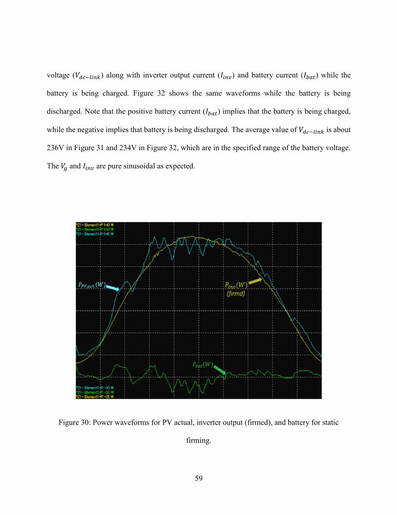
Figure 30 shows the experimental waveforms of the PV output power, the inverter output power
(firmed), and the battery power, while charging and discharging for the static PV firming system.
The timeline for the waveforms is scaled down to around half an hour. So, the rates of fluctuations
have been taken out of consideration. Since the 𝑃𝑃𝑉,𝑎𝑐𝑡 (blue curve) has been changed manually
using the Solar Array Simulator, the PV output power curve does not display as much fluctuation
as real-time power. However, the charging/discharging control algorithm is verified, since the 𝑃𝑖𝑛𝑣
(yellow) is following the generated PV reference power. The 𝑃𝑏𝑎𝑡 is either positive indicating that
the battery is discharging power to the grid (𝑃𝑃𝑉,𝑎𝑐𝑡 is greater than the generated PV reference), or
negative indicating that the battery is being charged from the PV (𝑃𝑃𝑉,𝑎𝑐𝑡 is less than the generated
PV reference). Figure 31 shows experimental waveforms of the grid voltage (𝑉𝑔), DC-link (battery)
Description
Nominal 12VCycle 14.5~14.9VFloat 13.6~13.8V
1.3Ah
Sealed Lead Acid (AGM -
Absorbent Glass Mat)
Length 97 (3.82)
Wedth 43 (1.69)
Height 52 (2.05)
Total Height 58 (2.28)
0.6 (1.32)
T1-A
Specifications
Rated Capacity 77°F(25°C)
Terminal
Chemistry
Dimension
s
(mm/inch)
Approx. Weight (kg/Ibs)
Voltage
59
voltage (𝑉𝑑𝑐−𝑙𝑖𝑛𝑘) along with inverter output current (𝐼𝑖𝑛𝑣) and battery current (𝐼𝑏𝑎𝑡) while the
battery is being charged. Figure 32 shows the same waveforms while the battery is being
discharged. Note that the positive battery current (𝐼𝑏𝑎𝑡) implies that the battery is being charged,
while the negative implies that battery is being discharged. The average value of 𝑉𝑑𝑐−𝑙𝑖𝑛𝑘 is about
236V in Figure 31 and 234V in Figure 32, which are in the specified range of the battery voltage.
The 𝑉𝑔 and 𝐼𝑖𝑛𝑣 are pure sinusoidal as expected.
Figure 30: Power waveforms for PV actual, inverter output (firmed), and battery for static
firming.

60
Figure 31: Grid voltage (Vg), DC-link voltage (Vdc-link), inverter output current (Iinv), and battery
current (Ibat) waveforms while the battery is being charged.

61
Figure 32: Grid voltage (Vg), DC-link voltage (Vdc-link), inverter output current (Iinv), and battery
current (Ibat) waveforms while the battery is being discharged.
3.6 Storage Capacity Sizing Analysis for the Static PV Reference
Energy data was collected for two PV modular systems with 600W total power in [60], where each
system consists of a PV panel and grid-tied microinverter. A monthly average PV reference power
is generated and passed through another algorithm of charging/discharging control where the static
PV firming algorithm is assumed to be applied. Based on this assumption, the PV energy is
calculated and analyzed for each month to conclude with an average usable storage capacity.
First, since the data collected is for PV power, energy must be calculated as follows.
62
𝐸𝑃𝑉 = 𝑃𝑃𝑉 ∙ 𝑡 ( 15 )
where,
- 𝐸𝑃𝑉: PV energy in watt-hour.
- 𝑃𝑃𝑉: PV power in watt.
- 𝑡: time in hour.
In order to determine the average battery capacity for each month, the average PV energy
(𝑬𝑃𝑉,𝑎𝑣𝑔), maximum PV energy (𝑬𝑃𝑉,𝑚𝑎𝑥), and minimum PV energy (𝑬𝑃𝑉,𝑚𝑖𝑛) are calculated
using equations ( 16 ) through ( 24 ).
Equation ( 16 ) defines the total average PV energy which is calculated by integrating the average
energy for every minute (𝐸𝑃𝑉,𝑎𝑣𝑔𝑚𝑛 ) given in ( 17 ) and ( 18 ). 𝐸𝑃𝑉,𝑎𝑣𝑔
𝑚𝑛 is calculated by averaging the
energy at that moment over one complete month.
𝑬𝑃𝑉,𝑎𝑣𝑔 = ∫ 𝐸𝑃𝑉,𝑎𝑣𝑔(𝑡)𝑑𝑡 ( 16 )
𝐸𝑃𝑉,𝑎𝑣𝑔(𝑡) = {𝐸𝑎𝑣𝑔𝑚1 , 𝐸𝑎𝑣𝑔
𝑚2 , … , 𝐸𝑎𝑣𝑔𝑚𝑘 } ( 17 )
𝐸𝑃𝑉,𝑎𝑣𝑔𝑚𝑛 =
∑ (𝐸𝑎𝑣𝑔𝑚𝑛 (𝑑𝑛))
𝑑𝑙𝑑1
𝑙 ( 18 )
where,

63
- 𝑚1, 𝑚2, 𝑚3 … 𝑚𝑘: correspond to the minutes over a day.
- 𝑘: is equal to 1440, which is the total minutes in each day.
- 𝑑1, 𝑑2, 𝑑3 … 𝑑𝑙: correspond to the days over each month.
- 𝑙: is the last day of each month.
- 𝐸𝑃𝑉,𝑎𝑣𝑔𝑚𝑛 : is the PV energy at the nth minute averaged correspondingly over a month.
Similar method is applied for the maximum PV energy (𝑬𝑃𝑉,𝑚𝑎𝑥) and the minimum PV energy
(𝑬𝑃𝑉,𝑚𝑖𝑛), as follows.
𝑬𝑃𝑉,𝑚𝑎𝑥 = ∫ 𝐸𝑃𝑉,𝑚𝑎𝑥(𝑡)𝑑𝑡 ( 19 )
𝐸𝑃𝑉,𝑚𝑎𝑥(𝑡) = {𝐸𝑃𝑉,𝑚𝑎𝑥𝑚1 , 𝐸𝑃𝑉,𝑚𝑎𝑥
𝑚2 , … , 𝐸𝑃𝑉,𝑚𝑎𝑥𝑚𝑘 } ( 20 )
𝐸𝑃𝑉,𝑚𝑎𝑥𝑚𝑛 = 𝑀𝑎𝑥𝑑1
𝑑𝑙 {𝐸𝑃𝑉,𝑚𝑎𝑥𝑚𝑛 (𝑑𝑛)} ( 21 )
𝑬𝑃𝑉,𝑚𝑖𝑛 = ∫ 𝐸𝑃𝑉,𝑚𝑖𝑛(𝑡)𝑑𝑡 ( 22 )
𝐸𝑃𝑉,𝑚𝑖𝑛(𝑡) = {𝐸𝑃𝑉,𝑚𝑖𝑛𝑚1 , 𝐸𝑃𝑉,𝑚𝑖𝑛
𝑚2 , … , 𝐸𝑃𝑉,𝑚𝑖𝑛𝑚𝑘 } ( 23 )
𝐸𝑃𝑉,𝑚𝑖𝑛𝑚𝑛 = 𝑀𝑖𝑛𝑑1
𝑑𝑙 {𝐸𝑃𝑉,𝑚𝑖𝑛𝑚𝑛 (𝑑𝑛)} ( 24 )

64
Examples are plotted in Figure 33 for two different months in 2016. The total average PV energy
is around 3.2kWh in Feb, and around 2.7kWh in June. The rest of months are given in Appendix
B.

65
(a)
(b)
Figure 33: Average, maximum, and minimum PV energy for month of (a) Feb. 2016 and (b) Jun.
2016.
66
Now, the average usable storage capacity can be calculated where the PV output profile is
statistically assumed to be firmed on the average PV power. Also, it is assumed to have both
maximum and minimum energy on same day. So, the average PV energy curve (𝐸𝑃𝑉,𝑎𝑣𝑔(𝑡)) as
shown in Figure 33, is considered to be the PV firming reference power. The area between the
maximum PV energy curve (𝐸𝑃𝑉,𝑚𝑎𝑥(𝑡)) and the 𝐸𝑃𝑉,𝑎𝑣𝑔(𝑡) is considered to be the average surplus
PV energy stored in the storage (𝐸𝑃𝑉,𝑠𝑢𝑟𝑝𝑙𝑢𝑠). However, the area between the 𝐸𝑃𝑉,𝑎𝑣𝑔(𝑡) and the
minimum PV energy curve (𝐸𝑃𝑉,𝑚𝑖𝑛(𝑡)) is considered to be the average deficient PV energy taken
from the storage (𝐸𝑃𝑉,𝑑𝑒𝑓𝑖𝑐𝑖𝑒𝑛𝑡). The difference between 𝐸𝑃𝑉,𝑠𝑢𝑟𝑝𝑙𝑢𝑠 and 𝐸𝑃𝑉,𝑑𝑒𝑓𝑖𝑐𝑖𝑒𝑛𝑡 is defined to
be the average usable storage (battery) capacity (𝐸𝑏𝑎𝑡,𝑐𝑎𝑝) needed to maintain the static PV firming
output profile, which is given in ( 25 ).
𝐸𝑏𝑎𝑡,𝑐𝑎𝑝 = |𝐸𝑃𝑉,𝑠𝑢𝑟𝑝𝑙𝑢𝑠 − 𝐸𝑃𝑉,𝑑𝑒𝑓𝑖𝑐𝑖𝑒𝑛𝑡| ( 25 )
where,
𝐸𝑃𝑉,𝑠𝑢𝑟𝑝𝑙𝑢𝑠 = ∫ 𝐸𝑃𝑉,𝑚𝑎𝑥(𝑡)𝑑𝑡 − ∫ 𝐸𝑃𝑉,𝑎𝑣𝑔(𝑡)𝑑𝑡 = 𝐸𝑃𝑉,𝑚𝑎𝑥 − 𝐸𝑃𝑉,𝑎𝑣𝑔 ( 26 )
𝐸𝑃𝑉,𝑑𝑒𝑓𝑖𝑐𝑖𝑒𝑛𝑡 = ∫ 𝐸𝑃𝑉,𝑎𝑣𝑔(𝑡)𝑑𝑡 − ∫ 𝐸𝑃𝑉,𝑚𝑖𝑛(𝑡)𝑑𝑡 = 𝐸𝑃𝑉,𝑎𝑣𝑔 − 𝐸𝑃𝑉,𝑚𝑖𝑛 ( 27 )
Figure 34 represents a summary for the analyzed average storage capacity that is assumed to be
needed according to the data collected for each month.
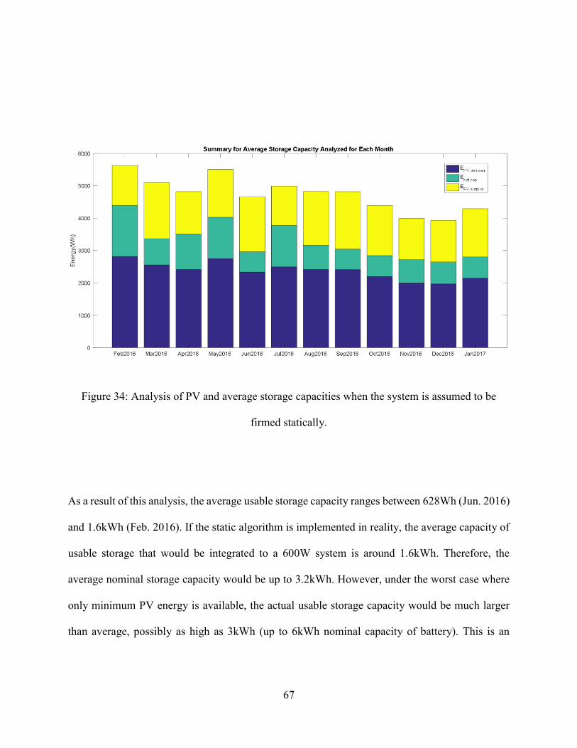
67
Figure 34: Analysis of PV and average storage capacities when the system is assumed to be
firmed statically.
As a result of this analysis, the average usable storage capacity ranges between 628Wh (Jun. 2016)
and 1.6kWh (Feb. 2016). If the static algorithm is implemented in reality, the average capacity of
usable storage that would be integrated to a 600W system is around 1.6kWh. Therefore, the
average nominal storage capacity would be up to 3.2kWh. However, under the worst case where
only minimum PV energy is available, the actual usable storage capacity would be much larger
than average, possibly as high as 3kWh (up to 6kWh nominal capacity of battery). This is an
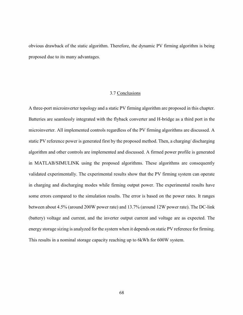
68
obvious drawback of the static algorithm. Therefore, the dynamic PV firming algorithm is being
proposed due to its many advantages.
3.7 Conclusions
A three-port microinverter topology and a static PV firming algorithm are proposed in this chapter.
Batteries are seamlessly integrated with the flyback converter and H-bridge as a third port in the
microinverter. All implemented controls regardless of the PV firming algorithms are discussed. A
static PV reference power is generated first by the proposed method. Then, a charging/ discharging
algorithm and other controls are implemented and discussed. A firmed power profile is generated
in MATLAB/SIMULINK using the proposed algorithms. These algorithms are consequently
validated experimentally. The experimental results show that the PV firming system can operate
in charging and discharging modes while firming output power. The experimental results have
some errors compared to the simulation results. The error is based on the power rates. It ranges
between about 4.5% (around 200W power rate) and 13.7% (around 12W power rate). The DC-link
(battery) voltage and current, and the inverter output current and voltage are as expected. The
energy storage sizing is analyzed for the system when it depends on static PV reference for firming.
This results in a nominal storage capacity reaching up to 6kWh for 600W system.

69
CHAPTER 4: DYNAMIC PV FIRMING ALGORITHM
4.1 Introduction
This chapter proposes a new dynamic PV firming algorithm using the same topology proposed in
previous chapter. The main reason that this algorithm was developed is to optimize the storage
capacity sizing. The results support the need for the dynamic PV firming algorithm. Section 4.2
presents the proposed dynamic PV firming system that consists of an algorithm for generating
dynamic PV reference power and an algorithm for battery charging/discharging control.
MATLAB/SIMULINK simulations are presented in Section 4.3, along with relevant waveforms.
Section 4.4 shows an experimental validation of the proposed schemes.
4.2 Proposed Dynamic PV Firming System
4.2.1 Dynamic PV Reference Generation Algorithm
In the proposed dynamic PV reference generation algorithms, one static reference must be
computed and coded. Several power levels are generated accordingly. By comparing the actual PV
power to the power levels, the PV reference power is generated dynamically.

70
The dynamic reference generation algorithm depends on three main factors. The first factor is the
maximum PV reference curve (𝑃𝑟𝑒𝑓,𝑚𝑎𝑥) formulated in ( 9 ) and ( 10 ) which generates several
power levels. It can be assumed as a map for the final generated reference power. It changes
monthly based on the analysis of collected data at Central Florida (example) location [60]. The
second factor is the fluctuation factor (ls). It controls the smoothness of the generated reference
curve and determines the number of comparable power levels (No. of power levels = 1/ ls) as
shown in Figure 35. In other words, the ls is indicative of the fluctuations/ smoothness rate. The
lower the ls, the higher the number of comparing power levels. By increasing the number of power
levels, the generated PV reference will have more rapid changes. This is because there are more
power levels (references) needing to be tracked which results in decreased smoothness. Since the
power level curves are generated by the 𝑃𝑟𝑒𝑓,𝑚𝑎𝑥, the only data saved in the memory is 𝑃𝑟𝑒𝑓,𝑚𝑎𝑥.
The third factor is the slew rate factor (𝜎𝑓). It dampens the ramp rate of the PV actual power
(𝑃𝑃𝑉,𝑎𝑐𝑡) against abrupt changes, as well as contributing to the smoothness. In other words, the 𝜎𝑓
determines where the generated PV reference is located according to either the PV actual power
change difference (𝑑(𝑖)) or the difference between the current 𝑃𝑃𝑉,𝑎𝑐𝑡 and the previous 𝑃𝑃𝑉,𝑟𝑒𝑓
(𝑑𝑓(𝑖)). The 𝜎𝑓 is defined as a factor of a slope equation as in ( 28 ) or ( 29 ) for either the 𝑑(𝑖) or
the 𝑑𝑓(𝑖), respectively.
𝜎𝑓𝑃𝑟𝑒𝑓,𝑚𝑎𝑥(𝑖) =𝑑(𝑖)
∆𝑡 ( 28 )
𝜎𝑓𝑃𝑟𝑒𝑓,𝑚𝑎𝑥(𝑖) =𝑑𝑓(𝑖)
∆𝑡 ( 29 )

71
𝑑(𝑖) = 𝑃𝑃𝑉,𝑎𝑐𝑡(𝑖) − 𝑃𝑃𝑉,𝑎𝑐𝑡(𝑖 − 1) ( 30 )
𝑑𝑓(𝑖) = 𝑃𝑃𝑉,𝑎𝑐𝑡(𝑖) − 𝑃𝑃𝑉,𝑟𝑒𝑓(𝑖 − 1) ( 31 )
where,
- 𝑑(𝑖) is the PV actual power change difference as defined in ( 30 ).
- 𝑑𝑓(𝑖) is the difference between the current 𝑃𝑃𝑉,𝑎𝑐𝑡 and the previous 𝑃𝑃𝑉,𝑟𝑒𝑓 as given in
(31).
- ∆𝑡 is the time difference and is assumed to be 1 minute since data changes every minute.
- 𝑃𝑃𝑉,𝑎𝑐𝑡(𝑖) is the current value of the actual PV power.
- 𝑃𝑃𝑉,𝑎𝑐𝑡(𝑖 − 1) is the previous value of the actual PV power.
- 𝑃𝑃𝑉,𝑟𝑒𝑓(𝑖 − 1) is the previous value of the generated PV reference power.

72
Figure 35: The maximum PV reference power with generated power levels.

73
Figure 36: Proposed algorithm for dynamic PV reference power generation.
Figure 36 illustrates the flowchart for the dynamic 𝑃𝑃𝑉,𝑟𝑒𝑓 generation algorithm. The algorithm
begins by comparing the current value of the 𝑃𝑃𝑉,𝑎𝑐𝑡(𝑖) with 𝑃𝑟𝑒𝑓,𝑚𝑎𝑥, designated as state 1. If
𝑃𝑃𝑉,𝑎𝑐𝑡(𝑖) is greater than or equal to 𝑃𝑟𝑒𝑓,𝑚𝑎𝑥, the generated 𝑃𝑃𝑉,𝑟𝑒𝑓 will be maintained to 𝑃𝑟𝑒𝑓,𝑚𝑎𝑥.
State 2, state 3, and state 4 depend on two variables: the PV actual power change difference (𝑑(𝑖))
Start
PPV,act(i) Pref,max(i)
PPV,ref(i)=Pref,max(i)
NoYes
|df(i)| σf·Pref,max(i)
|d(i)| σf·Pref,max(i)
OR
| ( )|> , ( )& | ( , (
| ( , ( OR
| ( )|> , ( )& | ( , (
( , (
Yes
No
Yes No
|d(i)| σf·Pref,max(i)
Locate
[PPV,act(i)]
Deploy PV, ( ) on closest layer
to , ( )
Yes
Deploy PV, ( ) on closest layer to
[ , ( )-d(i)]
Locate
[PPV,act(i)-d(i)]
No
State 1
State 2
State 3
State 4

74
in (29); and, the difference between the current 𝑃𝑃𝑉,𝑎𝑐𝑡 and the previous 𝑃𝑃𝑉,𝑟𝑒𝑓, which is 𝑑𝑓(𝑖) in
(30). First variable of 𝑑(𝑖) determines the ramp rate of the current PV actual power (𝑃𝑃𝑉,𝑎𝑐𝑡(𝑖))
compared to the previous PV actual power value (𝑃𝑃𝑉,𝑎𝑐𝑡(𝑖 − 1)). This is the actual power change
per minute. It is named actual-actual ramp rate. The second variable of 𝑑𝑓(𝑖) determines the ramp
rate of the 𝑃𝑃𝑉,𝑎𝑐𝑡(𝑖) compared to the previous PV generated reference power (𝑃𝑃𝑉,𝑟𝑒𝑓(𝑖 − 1)). It
is named actual-reference ramp rate. If 𝑃𝑃𝑉,𝑎𝑐𝑡(𝑖) is below 𝑃𝑟𝑒𝑓,𝑚𝑎𝑥, state 2 evaluates the
fluctuation by comparing the absolute value of 𝑑𝑓(𝑖) to the maximum fluctuating value in the
current time (𝜎𝑓 ∙ 𝑃𝑟𝑒𝑓,𝑚𝑎𝑥). This process determines how the current PV power is ramped up/down
compared to the previous PV firmed value. This shows how the actual-reference ramp rate is
changing currently. If |𝑑𝑓(𝑖)| is less than or equal to (𝜎𝑓 ∙ 𝑃𝑟𝑒𝑓,𝑚𝑎𝑥), it means that it has low ramp
rate. State 3 assures that the 𝑃𝑃𝑉,𝑎𝑐𝑡 is not fluctuating, by comparing 𝑑(𝑖) and 𝑑𝑓(𝑖) to (𝜎𝑓 ∙
𝑃𝑟𝑒𝑓,𝑚𝑎𝑥(𝑖)) or (𝜎𝑓 ∙ 𝑃𝑟𝑒𝑓,𝑚𝑎𝑥(𝑖 − 1)). State 3 is used to ascertain that the 𝑃𝑃𝑉,𝑎𝑐𝑡(𝑖) is consistent.
If state 2 is false, another comparison between d(i) and (𝜎𝑓 ∙ 𝑃𝑟𝑒𝑓,𝑚𝑎𝑥(𝑖)) is calculated to assure
that the 𝑃𝑃𝑉,𝑎𝑐𝑡(𝑖) is not fluctuating as in state 4. If either state 3 or state 4 is true, the location of
the 𝑃𝑃𝑉,𝑎𝑐𝑡(𝑖) is defined. Then, the generated 𝑃𝑃𝑉,𝑟𝑒𝑓 is deployed on the closest power level to the
current value of 𝑃𝑃𝑉,𝑎𝑐𝑡. If either state 3 or state 4 is false, which implies that the 𝑃𝑃𝑉,𝑎𝑐𝑡 has abrupt
change (high slew rate), the location of the [𝑃𝑃𝑉,𝑎𝑐𝑡(𝑖) − 𝑑(𝑖)] is defined. Then, the generated
𝑃𝑃𝑉,𝑟𝑒𝑓 is deployed on the closest power level to the current value of [𝑃𝑃𝑉,𝑎𝑐𝑡(𝑖) − 𝑑(𝑖)].

75
Figure 37 illustrates two examples of dynamic PV firming reference generation. They are
intermittencies for two different days. In Figure 37 (a), the slew rate factor (𝜎𝑓) is equal to 0.03
which means that the generated PV reference power (𝑃𝑃𝑉,𝑟𝑒𝑓) ramps by 3% of the maximum PV
reference power (𝑃𝑟𝑒𝑓,𝑚𝑎𝑥) curve or less. The fluctuation factor (ls) is equal to 0.25 implying that
there are 4 comparable power levels, where the output is as smooth as each power level. In Figure
37 (b), the 𝑃𝑃𝑉,𝑟𝑒𝑓 ramps by 7% of the 𝑃𝑟𝑒𝑓,𝑚𝑎𝑥 curve or less. The PV actual power (𝑃𝑃𝑉,𝑎𝑐𝑡) is
being compared to 5 different power levels.
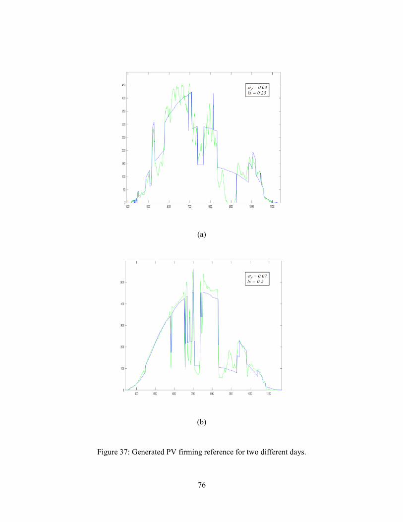
76
(a)
(b)
Figure 37: Generated PV firming reference for two different days.

77
4.2.2 Battery Charging/ Discharging Algorithm
As a second step in the PV firming process, the generated dynamic PV reference profile is used in
another algorithm of PV firming battery charge/discharge control (see Figure 38) to produce the
final power profile. This algorithm is identical to the PV-firming section in Figure 26 presented in
Chapter 3.

78
ccc
Figure 38: The algorithm flowchart for the PV firming battery charge/discharge control
4.3 Simulation Results
Simulations are carried out in MATLAB/Simulink to validate the proposed static PV-firming
algorithm on the grid-tied two-stage battery-integrated topology shown earlier in Figure 18. Power
waveforms for the PV actual power (𝑃𝑃𝑉,𝑎𝑐𝑡), the inverter stage output power (𝑃𝑖𝑛𝑣), and the battery
power (𝑃𝑏𝑎𝑡) for the dynamic PV firming microsystem are shown in Figure 39. While the
simulation in MATLAB/Simulink takes a long time to perform the calculations, the timeline for
79
the waveforms is scaled down to 24 seconds. Thus, the rates of fluctuations are taken out of
consideration. The battery power (𝑃𝑏𝑎𝑡) is either positive indicating that the battery is discharging
power to the grid, or negative indicating that the battery is being charged from the PV. The DC-
link voltage (𝑉𝑑𝑐−𝑙𝑖𝑛𝑘), inverter output current (𝐼𝑖𝑛𝑣), and inverter reference RMS current (𝐼𝑖𝑛𝑣,𝑟𝑒𝑓)
are as shown in Figure 40. The 𝑉𝑑𝑐−𝑙𝑖𝑛𝑘 is between 210V to 245V, which is the battery voltage.
The 𝐼𝑖𝑛𝑣,𝑟𝑒𝑓 is equal to the RMS value of the sinusoidal 𝐼𝑖𝑛𝑣.
Figure 39: Power waveforms for PV actual (blue), firmed inverter output (red), and battery
(green) for the dynamic firming microsystem.

80
Figure 40: DC-link voltage (Vdc-link), inverter output current (Iinv), and inverter reference RMS
current (Iinv,ref) waveforms.
4.4 Experimental Results
To experimentally verify the proposed static PV-firming control algorithm, a 200W prototype is
built with specifications as shown in Table 5 in Section 3.5. The same prototype test set-up as in
the static algorithm experiment is applied.
Figure 41 shows the experimental voltage and current waveforms for the PV output power, inverter
output power (firmed), and the battery power while charging and discharging for the dynamic PV
firming system. The timeline for the waveforms is scaled down to around half an hour. So, the

81
rates of fluctuations have been out of consideration. Since the 𝑃𝑃𝑉,𝑎𝑐𝑡 (blue curve) has been
changed manually using the Solar Array Simulator, the PV output power curve does not
demonstrate as many fluctuations as it would with real-time power. However, the
charging/discharging control algorithm is verified since the 𝑃𝑖𝑛𝑣 (yellow) is following the
generated PV reference power. The 𝑃𝑏𝑎𝑡 is positive when the battery is discharging power to the
grid and the 𝑃𝑃𝑉,𝑎𝑐𝑡 is greater than the generated PV reference. The 𝑃𝑏𝑎𝑡 is negative when the
battery is being charged from the PV and the 𝑃𝑃𝑉,𝑎𝑐𝑡 is less than the generated PV reference. Figure
42 shows experimental waveforms of the grid voltage (𝑉𝑔), DC-link (battery) voltage (𝑉𝑑𝑐−𝑙𝑖𝑛𝑘)
along with inverter output current (𝐼𝑖𝑛𝑣) and battery current (𝐼𝑏𝑎𝑡) while the battery is being
charged. Figure 43 shows the same waveforms while the battery is being discharged. Note that the
positive battery current (𝐼𝑏𝑎𝑡) implies that the battery is being charged and similarly negative
implies that battery is being discharged. The average value of 𝑉𝑑𝑐−𝑙𝑖𝑛𝑘 is about 236V in Figure 42
and 234V in Figure 43, which are in the target range of the battery voltage. The 𝑉𝑔 and 𝐼𝑖𝑛𝑣 are
sinusoidal as expected.
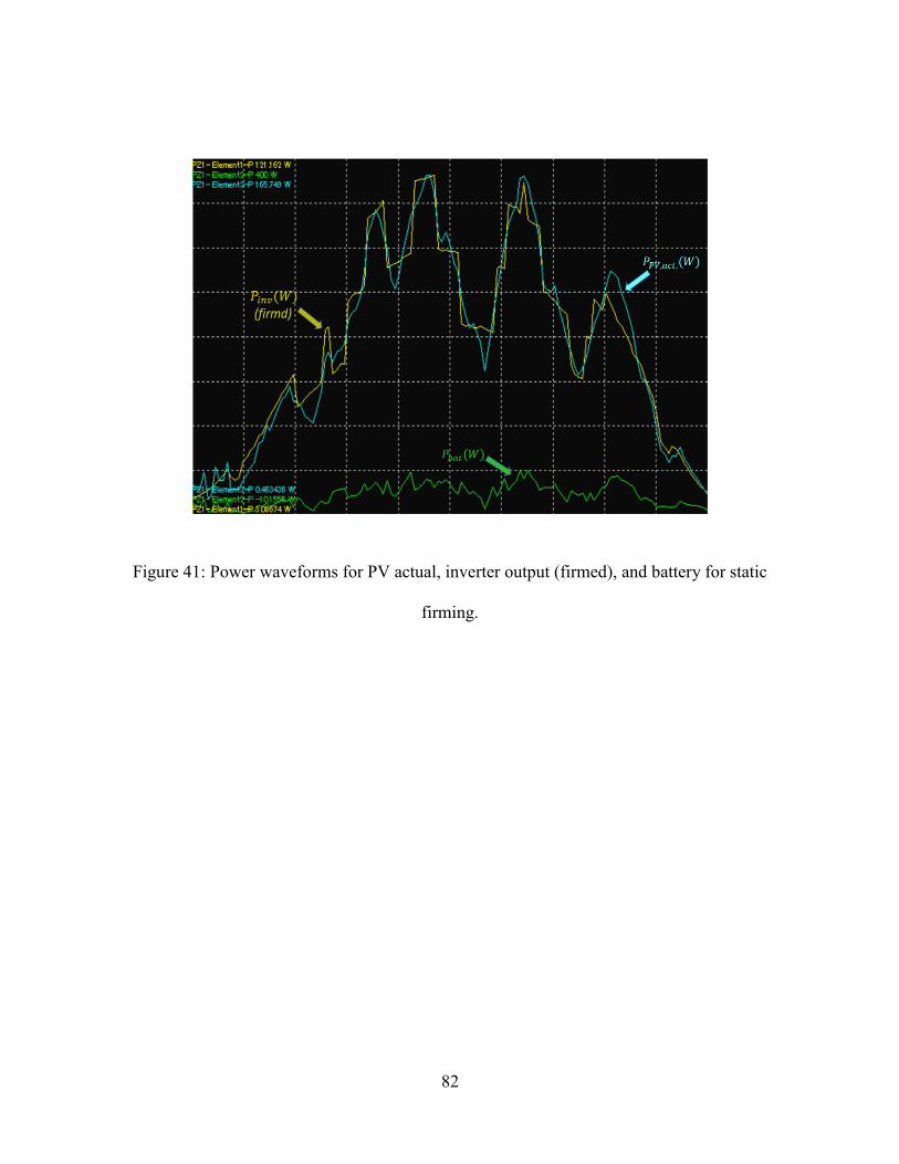
82
Figure 41: Power waveforms for PV actual, inverter output (firmed), and battery for static
firming.

83
Figure 42: Grid voltage (Vg), DC-link voltage (Vdc-link), inverter output current (Iinv), and battery
current (Ibat) waveforms while the battery is being charged.

84
Figure 43: Grid voltage (Vg), DC-link voltage (Vdc-link), inverter output current (Iinv), and battery
current (Ibat) waveforms while the battery is being discharged.
4.5 Storage Capacity Sizing Analysis for the Dynamic PV Reference
For the dynamic PV firming, the main factor that can determine the storage capacity sizing is the
fluctuation factor (ls). Therefore, in addition to controlling the smoothness of the output power
profile, there are other relationships between the number of power levels or the fluctuation factor
(ls) and the usable storage capacity (𝐸𝑏𝑎𝑡,𝑐𝑎𝑝), the surplus PV energy to be stored in the storage
(𝐸𝑃𝑉,𝑠𝑢𝑟𝑝𝑙𝑢𝑠), and the deficient PV energy (𝐸𝑃𝑉,𝑑𝑒𝑓𝑖𝑐𝑖𝑒𝑛𝑡). An example for analysis and discussion
is presented in Figure 44.

85
Figure 44: Power waveforms of PV actual (blue), PV reference/ firmed inverter output (red), and
battery (orange), such an example for a day in May 2016.
Initially, the slew rate factor (𝜎𝑓) must be fixed while the ls is being changed. Then, for every
adjustment of ls, the 𝐸𝑏𝑎𝑡,𝑐𝑎𝑝, the 𝐸𝑃𝑉,𝑠𝑢𝑟𝑝𝑙𝑢𝑠, and the 𝐸𝑃𝑉,𝑑𝑒𝑓𝑖𝑐𝑖𝑒𝑛𝑡 need to be calculated. There
are two different methods for calculating these energies.
The first method is to determine the difference between the PV actual power (𝑃𝑃𝑉,𝑎𝑐𝑡) and the
generated PV reference power (𝑃𝑃𝑉,𝑟𝑒𝑓) for every minute that 𝑃𝑃𝑉,𝑎𝑐𝑡 is greater/ less than 𝑃𝑃𝑉,𝑟𝑒𝑓.

86
The results are calculated in total to determine the energy. When 𝑃𝑃𝑉,𝑎𝑐𝑡 is greater than 𝑃𝑃𝑉,𝑟𝑒𝑓,
the 𝐸𝑃𝑉,𝑠𝑢𝑟𝑝𝑙𝑢𝑠 is resulted. Otherwise, it results the 𝐸𝑃𝑉,𝑑𝑒𝑓𝑖𝑐𝑖𝑒𝑛𝑡. The following equations represent
the calculations for this method.
𝐸𝑃𝑉,𝑠𝑢𝑟𝑝𝑙𝑢𝑠 = [∑ 𝑃𝑃𝑉,𝑎𝑐𝑡(𝑡)𝑡 𝛿𝑡 − ∑ 𝑃𝑃𝑉,𝑟𝑒𝑓(𝑡) 𝛿𝑡𝑡 ], 𝑃𝑃𝑉,𝑎𝑐𝑡 > 𝑃𝑃𝑉,𝑟𝑒𝑓 ( 32 )
𝐸𝑃𝑉,𝑑𝑒𝑓𝑖𝑐𝑖𝑒𝑛𝑡 = [∑ 𝑃𝑃𝑉,𝑟𝑒𝑓(𝑡) 𝛿𝑡𝑡 − ∑ 𝑃𝑃𝑉,𝑎𝑐𝑡(𝑡)𝑡 𝛿𝑡], 𝑃𝑃𝑉,𝑟𝑒𝑓 > 𝑃𝑃𝑉,𝑎𝑐𝑡 ( 33 )
The 𝐸𝑏𝑎𝑡,𝑐𝑎𝑝 is determined in (24).
The other method is to calculate the total positive and negative values for the battery power (𝑃𝑏𝑎𝑡),
where 𝑃𝑏𝑎𝑡 is the difference between 𝑃𝑃𝑉,𝑎𝑐𝑡 and 𝑃𝑃𝑉,𝑟𝑒𝑓.
𝐸𝑃𝑉,𝑠𝑢𝑟𝑝𝑙𝑢𝑠 = ∑ 𝑃𝑏𝑎𝑡(𝑡)𝑡 𝛿𝑡, 𝑃𝑏𝑎𝑡 > 0 ( 34 )
𝐸𝑃𝑉,𝑑𝑒𝑓𝑖𝑐𝑖𝑒𝑛𝑡 = − ∑ 𝑃𝑏𝑎𝑡(𝑡)𝑡 𝛿𝑡, 𝑃𝑏𝑎𝑡 < 0 ( 35 )

87
Figure 45: Analysis of PV and usable storage capacities when the system is firmed dynamically.
As shown in Figure 45, the fluctuation factor (ls) or the number of power levels (1/ ls) has an
obvious effect on the energy capacity of the storage. The relationship of the surplus PV energy
(𝐸𝑃𝑉,𝑠𝑢𝑟𝑝𝑙𝑢𝑠) and the deficient PV energy (𝐸𝑃𝑉,𝑑𝑒𝑓𝑖𝑐𝑖𝑒𝑛𝑡) to the ls seems linear until the ls is equal
to about 0.15, or there are about 7 comparable power levels. Thus, the usable storage capacity
(𝐸𝑏𝑎𝑡,𝑐𝑎𝑝) would have similar proportionality. Once the number of power levels decreases, or the
ls increases after that point, the 𝐸𝑃𝑉,𝑠𝑢𝑟𝑝𝑙𝑢𝑠 starts decreasing gradually with respect to the ls while

88
the 𝐸𝑃𝑉,𝑑𝑒𝑓𝑖𝑐𝑖𝑒𝑛𝑡 continues increasing linearly. Therefore, the 𝐸𝑏𝑎𝑡,𝑐𝑎𝑝 will be enlarged since the
PV energy is becoming much less sufficient. However, although decreasing the fluctuation factor
(ls) (increasing the number of power levels) minimizes the storage capacity, it affects the
smoothness negatively. As a result of this analysis, the storage capacity size can range from below
50Wh to above 200Wh (100Wh to 400Wh - nominal capacity value).
Figure 46 and Figure 47 illustrate the power waveforms for the example shown in Figure 44. Here,
the fluctuation rate is decreased by increasing the fluctuation factor (ls). So, the conclusion is that
the ls makes a trade-off between the fluctuation rates and the storage capacity sizing.

89
Figure 46: Power waveforms for same example shown in Figure 44 but with different fluctuation
factor (ls=0.1).

90
c
Figure 47: Power waveforms for same example shown in Figure 28 but with different fluctuation
factor (ls=0.3)).
4.6 Conclusions
Algorithms and analysis for a dynamic PV firming microsystem are proposed using a three-port
microinverter topology in this chapter. Batteries are seamlessly integrated with the flyback
converter and H-bridge inverter as a third port in the microinverter. According to the analysis
results for storage capacity sizing when the static algorithm is applied, the value of this novel
dynamic PV reference generation algorithm for PV firming is supported. As a first step, a static

91
PV maximum reference power is generated by the proposed method in chapter 3. Then, from that
reference, several power levels are assumed to generate final dynamic PV reference. This results
in an output power profile that can demonstrates minimal ramp-rate and reduced storage capacity.
In the final step of PV firming, the output of the dynamic PV reference generation algorithm
becomes an input of the charging/discharging algorithm to control the battery power. A PV firmed
power profile is generated first in MATLAB/ SIMULINK using the proposed algorithms which
are also validated experimentally. The experimental results show that the PV firming system can
operate in charging and discharging modes while firming output power. The experimental results
have some errors compared to the simulation results. The error is based on the power rates. It
ranges between about 4.5% (around 200W power rate) and 13.7% (around 12W power rate). The
DC-link (battery) voltage and current, and the inverter output current and voltage are as expected.
Finally, the sizing of the storage capacity is analyzed for the system when it depends on dynamic
PV reference for firming. This results in a nominal storage capacity changing form about 100Wh
to 400Wh for 600W system.

92
CHAPTER 5: DUAL OPTIMIZATION FOR THE INVERTION STAGE
5.1 Introduction
The H-bridge sinusoidal pulse-width modulation (SPWM) inverter is immensely used in numerous
applications such as grid-tied PV inverters [61], [61], [62], [62], and [63], uninterruptible power
supplies (UPS) [64], motor drives [65], [66], and active filters [67]. There are strict standards of
the permissible amount of harmonics that an inverter is allowed to generate in many of these
applications [68], [69]. Also, the high frequency SPWM is currently the most vastly used technique
to control the switches of the H-bridge inverter. The switching frequencies that are employed in
the SPWM must be well above the fundamental frequency. Although the switching loss in the
inverter is proportional to switching frequency, inductor DC loss and devices conduction losses
are proportional to the load power [70], [71].
The efficiency and the power quality of the SPWM full-bridge inverter can be improved without
modifying any component in the hardware. Varying the switching frequency over the fundamental
cycle is one way to increase the efficiency and optimize the power quality. A hysteresis current
controller for inverters is one such scheme of variable switching frequency methods that can
decrease the switching loss of the high current ripple area [72]. In [73], a variable switching
frequency scheme within a fundamental period is implemented to minimize the switching loss
while meeting the requirements of the total harmonic distortion (THD). Another method involves
doubling the switching frequency during the time when the ripple has increased [74]. Several

93
techniques of frequency tracking have been implemented in [75], [76], and [77] to optimize the
efficiency for different power conversion systems.
In this chapter, two algorithms to optimize the efficiency and the current THD for a conventional,
hard-switching H-bridge SPWM microinverter are proposed. Two different approaches are
discussed; dual tracking of optimum efficiency and THD algorithm, and perturbing and observing
the switching frequency while maintaining the minimum current THD for different loads. An
optimal switching frequency is proposed based on analysis of averaged loss power and THD over
a fundamental period for several loads. Section 5.2 presents an analysis of averaged total loss
modeling and calculation for the H-bridge SPWM microinverter. In Section 5.3, the proposed
algorithms for tracking the optimum switching frequency are presented. Section 5.4 shows the
experimental verifications followed by conclusions in Section 5.5.
5.2 Loss Modeling and Calculation
To accurately calculate the efficiency, all losses of both active and passive devices must be
calculated. As shown in Figure 48, there are eight active devices and three passive components
where each switch is driven by a single device. The left-side leg of the H-bridge microinverter,
which consists of Q1, Q3, D1, D2, D3, and D4, operates at high switching frequency (𝑓𝑠). The
right-side leg, which consists of Q2 and Q4, operates at frequencies as low as the fundamental
frequency (𝑓).

94
CBUS
Q1 Q2
Q4
D1
D3
Lo
Covo(t)
(Grid)
Q3 D2
D4
+
-
VB
US
Figure 48: H-bridge microinverter topology.
Because the objective is to analyze the switching frequency, the only passive component that will
be considered in the calculation is the output filter inductor (𝐿𝑜). According to the modes of
operation for the H-bridge inverter shown in Figure 49, both positive and negative half cycles have
same losses since they run using the same type and number of devices and components.

95
+
-
Q1/D3
D2
Q3/D4
D1
Mode 1 Mode 1Mode 2 Mode 2 Mode 3 Mode 3Mode 4 Mode 4
Q4
Q2
(a)

96
CBUS
Q1 Q2
Q4
D1
D3
Lo
Covo(t)
(Grid)
Q3 D2
D4
+
-
VB
US
Mode 1
CBUS
Q1 Q2
Q4
D1
D3
Lo
Covo(t)
(Grid)
Q3 D2
D4
+
-
VBU
S
Mode 2
CBUS
Q1 Q2
Q4
D1
D3
Lo
Covo(t)
(Grid)
Q3 D2
D4
+
-
VB
US
io(t)
Mode 3
CBUS
Q1 Q2
Q4
D1
D3
Lo
Covo(t)
(Grid)
Q3 D2
D4
+
-
VBU
S
io(t)
Mode 4
(b)
Figure 49: (a) Modes of operation waveforms. (b) Modes of operation circuits diagram.
So, calculating the losses during the positive half cycle only will provide adequate results.
Equation (35) represents the total instantaneous loss (𝑃𝑙𝑜𝑠𝑠𝑡𝑜𝑡𝑎𝑙) as a function of time. According

97
to (36), there are three types of losses, namely: inductor losses, conduction losses, and switching
losses. 𝑃𝐿𝐷𝐶 and 𝑃𝐿𝑐𝑜𝑟𝑒
are defined as inductor DC and core losses, respectively. The conduction
losses are distributed among the two operation modes of the SPWM topology, where 𝑃𝑄1𝑐𝑜𝑛 and
𝑃𝐷3𝑐𝑜𝑛 are when pair Q1/D3 devices are conducting and 𝑃𝐷2𝑐𝑜𝑛
′ and 𝑃𝑄4𝑐𝑜𝑛
′ are when pair Q4/D2
devices are conducting. 𝑃𝑄1𝑠𝑤and 𝑃𝑄4𝑠𝑤
are defined as the switching losses for Q1 and Q4,
respectively. Power losses equations and details are discussed in Appendix C.
𝑃𝑙𝑜𝑠𝑠𝑡𝑜𝑡𝑎𝑙(𝑡) = 𝑃𝐿𝐷𝐶
(𝑡) + 𝑃𝐿𝑐𝑜𝑟𝑒+ 𝑃𝑄1𝑐𝑜𝑛
(𝑡) + 𝑃𝐷3𝑐𝑜𝑛(𝑡) + 𝑃𝐷2𝑐𝑜𝑛
′ (𝑡)
+𝑃𝑄4𝑐𝑜𝑛
′ (𝑡) + 𝑃𝑄1𝑠𝑤(𝑡) + 𝑃𝑄4𝑠𝑤
(𝑡) ( 36 )
The instantaneous and averaged efficiencies are given in (37) and (38), respectively, where 𝑃𝑜 is
the average output power.
𝜂(𝑡) =𝑃𝑜−𝑃𝑙𝑜𝑠𝑠𝑡𝑜𝑡𝑎𝑙
(𝑡)
𝑃𝑜× 100% ( 37 )
𝜼 =2
𝑇∫ 𝜂(𝑡)
𝑇 2⁄
0𝑑𝑡 ( 38 )
Figure 50 presents the results for the power losses in percentage for the microinverter when the
switching frequency is 20kHz. The total switching loss percentage for this value of switching
frequency is 32%. This supports the need for proposing switching frequency tracking algorithm.

98
Figure 50: Power losses in percentage for the microinverter when the switching frequency is
20kHz.
5.3 Optimal Switching Frequency Tracking Algorithms
Both the THD and the efficiency are calculated by the microcontroller in order to implement the
proposed algorithms. There are two different approaches to optimize the H-bridge microinverter
used for the PV microinverter. One approach is to track the optimal switching frequency for
maximum efficiency under a certain THD. The other approach is to optimize the power quality of
the H-bridge microinverter by tracking the THD as a function of switching frequency.
23%
45%
32%
20kHz switching frequency
Total inductor loss Total conduction loss Total switching loss
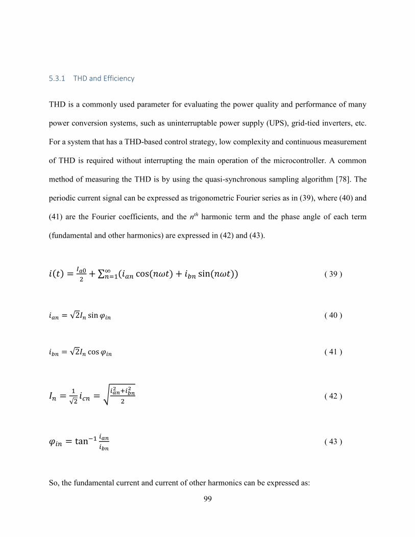
99
5.3.1 THD and Efficiency
THD is a commonly used parameter for evaluating the power quality and performance of many
power conversion systems, such as uninterruptable power supply (UPS), grid-tied inverters, etc.
For a system that has a THD-based control strategy, low complexity and continuous measurement
of THD is required without interrupting the main operation of the microcontroller. A common
method of measuring the THD is by using the quasi-synchronous sampling algorithm [78]. The
periodic current signal can be expressed as trigonometric Fourier series as in (39), where (40) and
(41) are the Fourier coefficients, and the nth harmonic term and the phase angle of each term
(fundamental and other harmonics) are expressed in (42) and (43).
𝑖(𝑡) =𝐼𝑎0
2+ ∑ (𝑖𝑎𝑛 cos(𝑛𝜔𝑡) + 𝑖𝑏𝑛 sin(𝑛𝜔𝑡))∞
𝑛=1 ( 39 )
𝑖𝑎𝑛 = √2𝐼𝑛 sin 𝜑𝑖𝑛 ( 40 )
𝑖𝑏𝑛 = √2𝐼𝑛 cos 𝜑𝑖𝑛 ( 41 )
𝐼𝑛 =1
√2𝑖𝑐𝑛 = √𝑖𝑎𝑛
2 +𝑖𝑏𝑛2
2 ( 42 )
𝜑𝑖𝑛 = tan−1 𝑖𝑎𝑛
𝑖𝑏𝑛 ( 43 )
So, the fundamental current and current of other harmonics can be expressed as:

100
𝐼𝑛(𝑡) = 𝑖𝑐𝑛 sin(𝑛𝜔𝑡 + 𝜑𝑖𝑛) = 𝑖𝑎𝑛 cos(𝑛𝜔𝑡) + 𝑖𝑏𝑛 sin(𝑛𝜔𝑡) ( 44 )
The total harmonic distortion is defined as:
𝑇𝐻𝐷𝑖 =√∑ 𝐼𝑛
2𝑁𝑛=2
𝐼1× 100% ( 45 )
The efficiency is measured by averaging the input and the output power of the H-bridge
microinverter by monitoring the sampled signals for input and output currents and voltages. The
averaged sampled power over one line period is expressed in (46).
�̅� =1
𝑇∑ 𝑖(𝑡) ∙ 𝑣(𝑡)𝑇
𝑡=0 ( 46 )
where
{𝑖(𝑡) = 𝐼𝑝𝑘 sin 𝜔𝑡
𝑣(𝑡) = 𝑉𝑝𝑘 sin 𝜔𝑡 ( 47 )
So, the efficiency is expressed as
𝜂 =𝑃𝑜̅̅ ̅
𝑃𝑖𝑛̅̅ ̅̅̅× 100% ( 48 )

101
where 𝑃�̅� and 𝑃𝑖𝑛̅̅ ̅̅ are the averaged sampled output and input powers over one line period,
respectively.
5.3.2 Approach 1: Dual Tracking of Optimum Efficiency and THD Algorithm
The optimal switching frequency is tracked using the search algorithm shown in Figure 51. This
algorithm optimizes the power quality and the efficiency of the H-bridge microinverter for
switching frequencies between 10 kHz and 100 kHz. The algorithm starts by setting the initial
switching frequency at 10 kHz for the current line cycle (𝑓𝑠,𝑘), and setting the first step value of
the switching frequency (𝑓𝑠𝑡𝑒𝑝) at 1 kHz, and the line cycle step (𝑘) at zero. Next, the maximum
required value for the percentage THD (α), which varies with different applications, is set at a
certain value (for example, α=2%). By monitoring the input and output voltages and currents, the
THD and efficiency (ɳ) are calculated using the microcontroller, and the switching frequency is
incremented every one complete cycle with a predetermined step size (µ).

102
Initializationk=0fs,k=10kHzfstep=1kHz
Calculate THDk
(eq. (45))
fs,k+1 = fs,k + µfstep
Set α
no
k = k + 1
END
yes
Calculate ηk
(eq. (48))
fs,k < 100kHz
Set fs,k such that
1) THDk < α; and
2) ηk = ηk,max
Set µ (eq. (49))
Figure 51: Proposed algorithm for dual tracking of optimum efficiency and THD values for the
H-bridge SPWM inverter (Approach 1).
The step size (µ) determines the incrementing value of the switching frequency and the
convergence speed. For example, if µ=2, the algorithm will need 46 iterations to calculate the THD
and efficiency (10kHz, 12kHz, 14kHz, …, 100kHz). Here, two different values of µ are chosen

103
for two different zones according to the THD analysis. These two values are given in (49). A small
µ is chosen for zone 1 where the rate of change between the THD and the switching frequency is
large, while in zone 2 the rate of change is low and hence a large µ is chosen, as shown in Figure
52.
Figure 52: Switching frequency zones and optimum THD point.
{10𝑘𝐻𝑧 ≤ 𝑓𝑠,𝑘 < 20𝑘𝐻𝑧, ⟹ 𝜇 = 2.5 (𝑧𝑜𝑛𝑒1)
20𝑘𝐻𝑧 ≤ 𝑓𝑠,𝑘 < 100𝑘𝐻𝑧, ⟹ 𝜇 = 5 (𝑧𝑜𝑛𝑒2) ( 49 )

104
5.3.3 Approach 2; Minimum THD Point Tracking Algorithm
The minimum THD point tracking, i.e. THDmin = αmin, is an algorithm implemented in the inverter
to continuously adjust the impedance seen by the microinverter output filter to keep the
microinverter output current delivering with, or close to, the minimum THD point under varying
loads. Figure 53 illustrates the algorithm flowchart.
This algorithm perturbs the switching frequency to ensure that the system operates at minimum
THD point (optimum point) on the THD curve, as shown in Figure 52.

105
SenseVin, Iin, Vo, Io
|THDk – THDk-1 |< αmin
END
fs,k+1 = fs,k + µfstep
Set µ (eq. (49))
k = k + 1
fs,k+1 = fs,k – µfstep
THD/ f < 0
yes
no
yes no
Initializationk=0fs,k=10kHzfstep=1kHz
Figure 53: Minimum THD point tracking algorithm (Approach 2).
In Figure 53, the algorithm starts by initializing the switching frequency and sensing the
input/output voltage and current to calculate the THD. If the absolute value of the change in the
THD between two successive iterations is below a minimum predefined value αmin, e.g. αmin=1%,
the algorithm terminates and the THD is considered minimum at that switching frequency. If the
absolute value of the change is above αmin, a value of µ is selected in a similar fashion as in the
algorithm in Figure 51. Based on the slope sign of the THD-switching frequency curve, the

106
frequency is incremented or decremented. The process only terminates if the variation in the THD
becomes below αmin. One remark on the approach is that by increasing the frequency resolution,
i.e. decreasing the step size, the value of αmin can be decreased and hence the algorithm becomes
more accurate. However, increasing the frequency resolution will reduce the speed of the
algorithm. For the frequency resolution in this research, which is 2.5 kHz (zone 1) or 5 kHz (zone
2), a value of 1% for αmin is found to be adequate.
5.4 Experimental Results
The DC/AC inverter stage (H-bridge) of the same prototype (200 W microinverter) used
previously for the PV-firming algorithms is used to validate the proposed techniques
experimentally, where the prototype specifications are shown in Table 5. Both efficiency and
power quality (THD) were measured as functions of both switching frequency and power rate.
Figure 54 illustrates the efficiency in terms of switching frequency for different power rates.
Noticeably, at high frequency, the efficiency is inversely proportional to the switching frequency
due to the high switching losses. Figure 55 illustrates the dependence of the THD on the switching
frequency at different power rates. The THD seems to have exponential relationship with the
switching frequency. Noticeably, the relationship between the efficiency as a function of switching
frequency and the load value shown (Figure 54) is nonlinear. Also, despite the linear relationship
between the THD and the load value at high frequencies (Figure 55), an almost parabolic curve is
shown for the THD as a function of switching frequency for a frequency range between 10 kHz

107
and 200 kHz. Hence, both the efficiency and the THD can be optimized by varying the switching
frequency as demonstrated.
Figure 54: Efficiency versus switching frequency at different loads.
95
95.5
96
96.5
97
97.5
98
98.5
99
0 50 100 150 200 250
Effi
cien
cy (
%)
Switching Frequency (kHz)
200W 150W 100W 50W

108
Figure 55: THD versus switching frequency at different loads.
Lastly, Figure 56 presents the results for optimal efficiency and THD values at each tested load
obtained using the algorithm of dual tracking described in Figure 51 (Approach 1). The efficiency
is maintained to maximum while the THD is limited to 4%. As for Approach 2 where the algorithm
tracks the minimum THD point tracking (Figure 53), the results are presented in Figure 57. The
THD is maintained to minimum (highest power quality) regardless of the efficiency.
0
2
4
6
8
10
12
14
16
18
20
0 50 100 150 200 250
THD
(%)
Switching Frequency (kHz)
200W 150W 100W 50W

109
Figure 56: Optimum switching frequencies for maximum efficiency and THD below 4%
(Approach 1).
98.07 98.78 98.58 98.16
3.81 2.98 2.39 1.67
50
1510
25
0
20
40
60
80
100
120
50 100 150 200
Power Rate (W)
Efficiency(%) THD(%) Switching Frequency (kHz)

110
Figure 57: Optimum switching frequencies for highest power quality at minimum THD
(Approach 2).
5.5 Conclusions
This chapter proposed two new algorithms to achieve dual optimization for an H-bridge SPWM
microinverter by an optimal switching frequency tracking technique. the first is dual tracking of
optimum efficiency and THD algorithm which tracks the optimal frequency for maximum
efficiency under certain percentage of THD, while the second is THD point tracking algorithm
which optimizes the power quality of the H-bridge microinverter by tracking the THD as a function
of switching frequency to maintain its optimum value.
97.67 98.45 98.51 98.14
3.72 2.16 1.76 1.66
75
50
30 30
0
20
40
60
80
100
120
50 100 150 200
Power Rate (W)
Efficiency(%) THD(%) Switching Frequency (kHz)

111
Using the proposed first technique (Approach 1), the power quality is improved by 60.1% for a 50
W load compared with a 20 kHz constant switching frequency inverter, while the efficiency is
maintained above 98%. As for the second technique (Approach 2), the achieved power quality
improvement is up to 63.9% compared to 20 kHz constant switching frequency inverter while the
efficiency is maintained very close to 98%.

112
CHAPTER 6: SUMMARY AND FUTUTRE WORKS
6.1 Summary
Energy demand is increasing worldwide. In recent decades, researchers have focused on harvesting
photovoltaic (PV) energy because it is a natural, clean, renewable source of power. Continuously
decreasing costs have made this option even more desirable. However, several challenges still exist
which limit its penetration into the grid. One challenge is the variable nature of solar irradiance
levels due to such things as passing clouds and storms. These variances lead to fluctuations in the
PV output power profile. This research proposes new approaches for smoothing the PV output and
increasing its penetration into the grid. It does this by using a panel-level system, which interfaces
with the PV, battery and grid. The system inversion stage is optimized by a switching frequency
tracking technique.
Chapter 3 presents and explains the topology used for the PV-firming, the implemented controls
regardless of the proposed algorithms, the static PV reference generation method, and the battery
charging/discharging algorithm. The topology is two-stage power conversion (DC/DC converter
(flyback) and DC/AC inverter (H-bridge)) micro-system, which integrates the battery as a third
port by a direct connection to the DC-link. It has the ability to transferring the battery energy
bidirectionally. Such controls must be implemented in this topology regardless of applying the
proposed PV firming algorithms. The MPPT (Maximum Power Point Tracking) control,
implemented in the DC/DC stage, ensures maximum power delivery by the PV. The phase locked

113
loop (PLL) control synchronizes the microinverter output with the grid waveforms. The DC-link
voltage regulation control (DCVR) balances the DC/DC output power and the DC/AC input
power, and sets the DC-link voltage. The output current regulation control (OCR) manages the
output current of the DC/AC stage. PLL, DCVR, and OCR are implemented throughout the
DC/AC stage. A static PV reference generation method is proposed for firming the output power
of the PV micro-system. The static reference is based on real-time data collected for PV
intermittency from two 300W PV modular systems including PV panels and a grid-tied
microinverter located in a specific region in East Florida. The generated static PV reference is
applied to an algorithm that controls the battery charge/discharge. The algorithm controls the
output inverter current, which controls the battery current. However, while this algorithm of the
battery charging/discharging control is being applied, the DC-link voltage regulation control
(DCVR) is disabled, where the voltage across the DC-link is fixed and equal to the battery voltage.
If the battery charging/discharging control is not applied, the battery will be disconnected and the
DCVR is enabled. Simulation and experimental results are presented to validate the approach of
the static PV firming algorithm. Finally, the storage capacity sizing for the system using the static
PV firming algorithm is determined and analyzed. The determination of the usable storage capacity
lies in calculating the average, maximum, and minimum energy for the PV. The surplus and
deficient energy are compared to the static reference. This analysis shows that the average capacity
of usable storage integrated to a 600W system is about 1.6kWh, where the nominal value is up to
3.2kWh. When PV energy is at a minimum (worst case), the usable storage capacity might reach
to 3kWh (about 6kWh nominal value). This supports the need for the dynamic PV firming
algorithm proposed in this research.

114
Chapter 4 discusses the most important contribution in this research, which is the dynamic PV
firming algorithm. To dynamically firm the output profile of the PV micro-system, a novel
algorithm is proposed to generate a dynamic PV reference power. Unlike conventional methods
(e.g. moving average), this algorithm does not require that one-hour previous data of solar
irradiance be calculated. In the proposed dynamic algorithm for PV firming, one smooth reference
is saved in the memory of the microcontroller. It is the maximum PV reference curve (𝑃𝑟𝑒𝑓,𝑚𝑎𝑥),
and thus multiple power levels of PV reference are generated. The number of power levels is
determined by the fluctuation factor (ls), where the number of power levels is equal to 1/ ls. The
power levels are tracked and compared to the actual PV power (𝑃𝑃𝑉,𝑎𝑐𝑡). Since there are no
complicated equations and calculations, the processing and implementation is very quick.
Furthermore, the ramp-rate of the actual PV power can be controlled from the abrupt changes by
the value of the slew rate factor (𝜎𝑓). The relationship between the fluctuation factor (ls) or the
number of power levels (1/ls), and battery sizing is also explored and discussed. The fluctuation
factor has effects on the usable storage capacity (𝐸𝑏𝑎𝑡,𝑐𝑎𝑝), the surplus PV energy to be stored in
the storage (𝐸𝑃𝑉,𝑠𝑢𝑟𝑝𝑙𝑢𝑠), and the deficient PV energy (𝐸𝑃𝑉,𝑑𝑒𝑓𝑖𝑐𝑖𝑒𝑛𝑡). Generally, the number of
power levels is inversely proportional to the usable storage capacity (𝐸𝑏𝑎𝑡,𝑐𝑎𝑝), as well as the
deficient PV energy (𝐸𝑃𝑉,𝑑𝑒𝑓𝑖𝑐𝑖𝑒𝑛𝑡) even though it has a parabolic relation with the storage
(𝐸𝑃𝑉,𝑠𝑢𝑟𝑝𝑙𝑢𝑠). However, the number of power levels is directly proportional to the smoothness of
the output PV profile. In other word, the fluctuation rate is decreased by increasing the fluctuation
factor (ls). As a result, the ls makes a trade-off between the fluctuation rates and the storage
capacity sizing. Once the dynamic PV reference is generated, another algorithm is used to control
the battery current and its charging or discharging status. This is the same as for the static method

115
discussed in chapter 3. Similarly, for the DCVR scenarios, it is disabled while the charging/
discharging control is being applied and enabled when the battery is disconnected. The charging/
discharging control for the dynamic PV firming approach is verified in simulation and
experimentally.
In chapter 5, two new approaches are proposed for optimizing an H-bridge SPWM microinverter
for PV modular level application without any hardware modification. The author begins by
creating a mathematical model for calculating the H-bridge losses. The results show that frequency
changing has a nonlinear relationship with different power rate efficiencies. Meanwhile, the
switching frequency makes trade-offs between the efficiency and the power quality. Implementing
the calculation of the total harmonic distortions (THD) and efficiency is discussed in section 5.3.1.
Using a tracking technique for an optimal switching frequency, dual optimization is achieved
which includes power efficiency and THD as a power quality factor. The first approach is based
on a tracking optimal switching frequency algorithm. It achieves dual optimization of maximum
efficiency and under a certain percentage of THD. The second approach optimizes the power
quality of the H-bridge microinverter using the proposed minimum THD point tracking algorithm
which is a function of the switching frequency. Both techniques are verified experimentally. Under
the first technique (Approach 1), the power quality for a 50 W load improved by 60.1% compared
to using a constant switching frequency of 20kHz at over 98% efficiency. The second technique
(Approach 2) achieved up to 63.9% improvement as compared to an inverter using a conventional
constant switching frequency of 20 kHz, while the power efficiency is maintained around 98%.

116
6.2 Future Works
Unique approaches for designing and implementing PV-firming algorithms and microinverter
power quality optimization were presented and studied analytically and experimentally in this
dissertation. More research can be done to optimize: the presented three-port topology; the
algorithms for the PV-firming and storage capacity sizing; and the approaches to the H-bridge
SPWM microinverter power efficiency and quality.
For the proposed topology, the battery is interfaced throughout the DC-link which has the
advantage of eliminating an additional stage for battery charging/ discharging conversion.
However, in this situation, the battery voltage must be as high as the DC-link voltage, which is an
uncommon voltage level for these types of applications. Furthermore, the DC/DC stage is a flyback
topology which is still a transformer-based topology that need to be optimized for higher
efficiency.
To further improve the performance of the PV-firming algorithms, several research points should
be considered. In this dissertation, there are some high ramp-rate fluctuations which in some cases
need to be filtered. Another research point is to find the optimal storage capacity based on the
proposed PV-firming algorithm for this specific 200W panel-level system or even for different
power level. For the battery charging/ discharging algorithm, an additional factor would be
considered in order to have a balanced case for charging/ discharging. In other words, the energy
consumed while the battery is being discharged should be equivalent to that energy acquired while
the battery is being charged.

117
For the H-bridge SPWM microinverter optimization in this dissertation, every line period has fixed
switching frequency and is tracked by two different algorithms. To further improve this technique
of switching frequency tracking, the scheme should be changed to have variable switching
frequency in every line period.

118
APPENDIX A: FSEC DATA SOURCE

119
A.1 What is FSEC?
Florida Solar Energy Center (FSEC) is a research institute of the University of Central Florida
(UCF) for researching and developing energy technologies that enhance the economy and
environment for the state of Florida and the nation. It was established in 1975 by the Florida
Legislature. It serves officially as research institute of the state’s energy. Several tasks that are
done by the center; research conducting, solar systems testing and certifying, developing education
programs for the public, students, and practitioners on the results of the research.
A.2 Data Collected for Modular PV System
FSEC has huge databases that collect data for several renewable energy technologies. One of the
databases that is used for this dissertation is for modular Photovoltaic (PV) system.
Data is collected from two 310W (measured at 304 and 305W) PV panels connected to
microinverters starting from Feb. 7th, 2016. The solar panels were in 5-degree tilt on roof. The
measurement of the system output energy is by a 1-minute resolution continental controls wattnode
power meter with pulse output (switch closure) using a calibration of 0.125 Wh/pulse. The channel
for the output power in Watt (W) is calculated as output energy (Wh) multiplied by 60.

120
A.3 Case Study-Data from FSEC
In the following figures examples for data collected by FSEC on April 11th, 2016. First figure
represents the PV energy measured as described in section A.2. The other figure is the PV power
collected on same day, where the power is resulted in multiplying the energy by 60 seconds as
explained in section A.2.

121

122
APPENDIX B: PV ENERGY PLOTS FOR TWELVE MONTHS

123

124

125
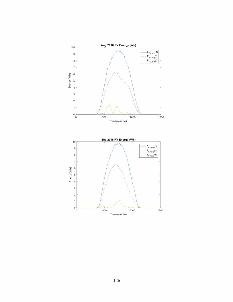
126

127

128

129
APPENDIX C: EQUATIONS OF THE INVERTER POWER LOSSES

130
According to (35), represents the total instantaneous loss (𝑃𝑙𝑜𝑠𝑠𝑡𝑜𝑡𝑎𝑙) as a function of time, there
are three types of losses, namely: inductor losses, conduction losses, and switching losses.
The inductor losses include DC and core losses, 𝑃𝐿𝐷𝐶 and 𝑃𝐿𝑐𝑜𝑟𝑒
, respectively, and are given in (45)
and (48).
𝑃𝐿𝐷𝐶(𝑡) = 𝐼𝐿_𝑟𝑚𝑠
2 𝑅𝐿_𝐷𝐶 ( 50 )
𝐼𝐿𝑟𝑚𝑠
2 (𝑡) = 𝑖𝑜2(𝑡) +
∆𝑖𝑝𝑝2
12 ( 51 )
∆𝑖𝑝𝑝(𝑡) =𝑉𝐵𝑈𝑆𝑇𝑠𝑚𝑎sin (𝜔𝑡)(1−𝑚𝑎 sin(𝜔𝑡))
𝐿𝑜 ( 52 )
where,
- 𝑅𝐿_𝐷𝐶: inductor DC resistance.
- ∆𝑖𝑝𝑝: current ripple [79].
- 𝑇𝑠 =1
𝑓𝑠; switching period.
- 𝑓𝑠: switching frequency.
- 𝑚𝑎 =𝑉𝑜_𝑝𝑒𝑎𝑘
𝑉𝐵𝑈𝑆; modulation index [80].
𝑃𝐿_𝑐𝑜𝑟𝑒 = 𝑃𝑣𝑉𝑒 ( 53 )

131
𝑃𝑣 =𝐶𝑚𝑓𝑠
𝑥𝐵𝑦(𝐶𝑡2𝑇2−𝐶𝑡1𝑇+𝐶𝑡)
1000 ( 54 )
where
- 𝑃𝑣: core loss in mW/cm3 as in [81][82].
- 𝑉𝑒: core effective volume [83].
The conduction losses are divided into two different modes. During mode 1, there are Q1, D3, and
Q4 conduction losses, 𝑃𝑄1𝑐𝑜𝑛, 𝑃𝐷3𝑐𝑜𝑛
, and 𝑃𝑄4𝑐𝑜𝑛, respectively, and are given in (50), (51), and
(52). During mode 2, there are D2 and Q4’ conduction losses, 𝑃𝐷2𝑐𝑜𝑛
′ and 𝑃𝑄4𝑐𝑜𝑛, respectively, and
are given in (53) and (54).
𝑃𝑄1𝑐𝑜𝑛(𝑡) =
𝑣𝑜(𝑡)
𝑉𝐵𝑈𝑆𝐼𝐿_𝑟𝑚𝑠
2 𝑅𝑄1_𝐷𝑆𝑜𝑛 ( 55 )
𝑃𝐷3𝑐𝑜𝑛(𝑡) =
𝑣𝑜(𝑡)
𝑉𝐵𝑈𝑆(0.23𝑖𝑜(𝑡) + 0.021𝐼𝐿𝑟𝑚𝑠
2 ) ( 56 )
𝑃𝑄4𝑐𝑜𝑛(𝑡) = 𝑃𝑄1𝑐𝑜𝑛
(𝑡) ( 57 )
𝑃𝐷2𝑐𝑜𝑛
′ (𝑡) = (1 −𝑣𝑜(𝑡)
𝑉𝐵𝑈𝑆) 𝐼𝐿_𝑟𝑚𝑠𝑉𝐷2_𝑓 ( 58 )
𝑃𝑄4𝑐𝑜𝑛
′ (𝑡) = (1 −𝑣𝑜(𝑡)
𝑉𝐵𝑈𝑆) 𝐼𝐿𝑟𝑚𝑠
2 𝑅𝑄4𝐷𝑆𝑜𝑛 ( 59 )

132
where,
- 𝑃𝐷3_𝑐𝑜𝑛 is according to [84].
- 𝑅𝑄1_𝐷𝑆𝑜𝑛 = 𝑅𝑄4_𝐷𝑆𝑜𝑛; drain to source on resistance [85].
- 𝑉𝐷2_𝑓: forward voltage as in [86].
The switching losses are based on the MOSFETs [87], Q1 and Q4, which are 𝑃𝑄1𝑠𝑤 and 𝑃𝑄4𝑠𝑤
,
respectively, and given in (55) and (56).
𝑃𝑄1𝑠𝑤(𝑡) = 0.5𝑉𝐵𝑈𝑆𝑖𝑜(𝑡)𝑓𝑠(𝑡𝑄1_𝐿𝐻 + 𝑡𝑄1_𝐻𝐿) ( 60 )
𝑃𝑄4𝑠𝑤(𝑡) = 0.5𝑉𝐵𝑈𝑆𝑖𝑜(𝑡)𝑓(𝑡𝑄4_𝐿𝐻 + 𝑡𝑄4_𝐻𝐿) ( 61 )
where,
- 𝑡𝑄1_𝐿𝐻/𝑡𝑄4_𝐿𝐻: pull-up switching time.
- 𝑡𝑄1_𝐻𝐿/𝑡𝑄4_𝐻𝐿: pull-down switching time.

133
LIST OF REFERENCES
[1] NREL, “Geospatial Data Science; Solar Maps,” National Renewable Energy Laboratory
(NREL). [Online]. Available: https://www.nrel.gov/gis/solar.html.
[2] “PV Intermittency Data,” Florida Solar Energy Center, University of Central Florida.
[Online]. Available: http://www.fsec.ucf.edu/en/.
[3] W. Jewell and R. Ramakumar, “The Effects of Moving Clouds on Electric Utilities with
Dispersed Photovoltaic Generation,” IEEE Trans. Energy Convers., vol. EC-2, no. 4, pp.
570–576, 1987.
[4] E. C. Kern and E. M. Gulachenski, “Cloud Effects on Distributed Photovoltaic Generation:
Slow Transients at the Gardner, Massachusetts Photovoltaic Experiment,” IEEE Trans.
Energy Convers., vol. 4, no. 2, pp. 184–190, 1989.
[5] A. Woyte, V. Van Thong, R. Belmans, and J. Nijs, “Voltage fluctuations on distribution
level introduced by photovoltaic systems,” IEEE Trans. Energy Convers., vol. 21, no. 1, pp.
202–209, 2006.
[6] D. L. Garrett and S. M. Jeter, “A Photovoltaic Voltage Regulation Impact Investigation
Technique: Part I - Model Development,” IEEE Trans. Energy Convers., vol. 4, no. 1, pp.
47–53, 1989.
[7] S. A. Zabalawi, G. Mandic, and A. Nasiri, “Utilizing Energy Storage with PV for

134
Residential and Commercial Use,” in 2008 34th Annual Conference of IEEE Industrial
Electronics (IECON), Orlando, FL, 2008, pp. 1045–1050.
[8] C. Trueblood et al., “PV Measures Up for Fleet Duty: Data From A Tennessee Plant Are
Used to Illustrate Metrics That Characterize Plant Performance,” IEEE Power Energy Mag.,
vol. 11, no. 2, pp. 33–44, 2013.
[9] M. J. E. Alam, K. M. Muttaqi, and D. Sutanto, “Mitigation of Rapid Voltage Variations
Caused by Passing Clouds in Distribution Networks with Solar PV Using Energy Storage,”
in 8th International Conference on Electrical and Computer Engineering: Advancing
Technology for a Better Tomorrow, ICECE 2014, 2014, no. 1, pp. 305–308.
[10] J. Jolmson, B. Schenkman, A. Ellis, J. Quiroz, and C. Lenox, “Initial Operating Experience
of the 1.2-MW La Ola Photovoltaic System,” in 2012 IEEE 38th Photovoltaic Specialists
Conference (PVSC) PART 2, 2012, pp. 1–6.
[11] NREL, “1-Second Global Horizontal Irradiance, Oahu, Hawaii.” [Online]. Available:
https://midcdmz.nrel.gov/oahu_archive/.
[12] S. Abdollahy, A. Mammoli, F. Cheng, A. Ellis, and J. Johnson, “Distributed Compensation
of A Large Intermittent Energy Resource in A Distribution Feeder,” in 2013 IEEE PES
Innovative Smart Grid Technologies Conference, ISGT 2013, 2013, pp. 1–6.
[13] D. Sayeef, Saad; Heslop, Simon; Cornforth, David; Moore, Tim; Percy, Steven; Ward, John;

135
Berry, Adam; Rowe, “Solar intermittency: Australia’s clean energy challenge.
Characterising the effect of high penetration solar intermittency on Australian electricity
networks,” CSIRO, Newcastle, 2012.
[14] H. Sugihara, K. Yokoyama, O. Saeki, K. Tsuji, and T. Funaki, “Economic and Efficient
Voltage Management Using Customer-Owned Energy Storage Systems in A Distribution
Network with High Penetration of Photovoltaic Systems,” IEEE Trans. Power Syst., vol.
28, no. 1, pp. 102–111, 2013.
[15] L. Bird, M. Milligan, D. Lew, L. Bird, M. Milligan, and D. Lew, “Integrating Variable
Renewable Energy : Challenges and Solutions Integrating Variable Renewable Energy :
Challenges and Solutions,” National Renewable Energy Laboratory (NREL), 2013.
[16] L. Chang, W. Zhang, S. Xu, and K. Spence, “Review on Distributed Energy Storage
Systems for Utility Applications,” CPSS Trans. POWER Electron. Appl., vol. 2, no. 4, pp.
267–276, 2017.
[17] H. Chen, T. Ngoc, W. Yang, C. Tan, and Y. Li, “Progress in electrical energy storage
system : A critical review,” Prog. Nat. Sci., vol. 19, no. 3, pp. 291–312, 2009.
[18] and A. S. D. O. M. Toledo, D. O. Filho, “Distributed photovoltaic generation and energy
storage systems: A review,” Renew. Sustain. Energy Rev., vol. 14, no. 1, pp. 506–511, 2010.
[19] S. Vazquez, S. M. Lukic, E. Galvan, L. G. Franquelo, and J. M. Carrasco, “Energy Storage

136
Systems for Transport and Grid Applications,” IEEE Trans. Ind. Electron., vol. 57, no. 12,
pp. 3881–3895, 2010.
[20] H. Zhao, Q. Wu, S. Hu, H. Xu, and C. N. Rasmussen, “Review of energy storage system
for wind power integration support,” Appl. Energy, vol. 137, no. 1, pp. 545–553, 2015.
[21] M. Yilmaz and P. T. Krein, “Review of Battery Charger Topologies , Charging Power
Levels , and Infrastructure for Plug-In Electric and Hybrid Vehicles,” IEEE Trans. Power
Electron., vol. 28, no. 5, pp. 2151–2169, 2013.
[22] W. Choi et al., “Reviews on Grid-Connected Inverter , Utility-Scaled Battery Energy
Storage System , and Vehicle-to-Grid Application – Challenges and Opportunities,” in 2017
IEEE Transportation Electrification Conference and Expo (ITEC), 2017, pp. 203–210.
[23] X. Luo, J. Wang, M. Dooner, and J. Clarke, “Overview of current development in electrical
energy storage technologies and the application potential in power system operation,” Appl.
Energy, vol. 137, no. 1, pp. 511–536, 2015.
[24] D. O. Akinyele and R. K. Rayudu, “Review of energy storage technologies for sustainable
power networks,” Sustain. Energy Technol. Assessments, vol. 8, no. 12, pp. 74–91, 2014.
[25] E. Barbour, I. G. Wilson, J. Radeliffe, Y. Ding, and Y. Li, “A review of pumped hydro
energy storage development in significant international electricity markets,” Renew.
Sustain. Energy Rev., vol. 61, no. 8, pp. 421–432, 2016.
137
[26] S. Briola, P. D. Marco, R. Gabbrielli, and J. Riccardi, “A novel mathematical model for the
performance assessment of diabatic compressed air energy storage systems including the
turbomachinery characteristic curves,” Appl. Energy, vol. 178, no. 9, pp. 758–772, 2016.
[27] S. F. Tie and C. W. Tan, “A review of energy sources and energy management system in
electric vehicles,” Renew. Sustain. Energy Rev., vol. 20, no. 4, pp. 82–102, 2013.
[28] M. J. E. Alam, K. M. Muttaqi, and D. Sutanto, “Mitigation of Rooftop Solar PV Impacts
and Evening Peak Support by Managing Available Capacity of Distributed Energy Storage
Systems,” IEEE Trans. Power Syst., vol. 28, no. 4, pp. 3874–3884, 2013.
[29] M. Bortolini, M. Gamberi, and A. Graziani, “Technical and Economic Design of
Photovoltaic and Battery Energy Storage System,” Energy Convers. Manag., vol. 86, pp.
81–92, 2014.
[30] X. Han, T. Ji, Z. Zhao, and H. Zhang, “Economic Evaluation of Batteries Planning in Energy
Storage Power Stations for Load Shifting,” Renew. Energy, vol. 78, pp. 643–647, 2015.
[31] Y. Zhang, A. Lundblad, P. E. Campana, and J. Yan, “Employing Battery Storage to Increase
Photovoltaic Self-sufficiency in a Residential Building of Sweden,” Energy Procedia, vol.
88, pp. 455–461, 2016.
[32] V. Fthenakis, J. E. Mason, and K. Zweibel, “The technical , geographical , and economic
feasibility for solar energy to supply the energy needs of the US,” Energy Policy, vol. 37,
138
pp. 387–399, 2009.
[33] F. Cucchiella, I. D. Adamo, and M. Gastaldi, “Photovoltaic Energy Systems with Battery
Storage for Residential Areas : An Economic Analysis International Panel on Climate
Change,” J. Clean. Prod., vol. 131, pp. 460–474, 2016.
[34] A. A. Solomon, D. Faiman, and G. Meron, “Appropriate Storage for High-Penetration Grid-
Connected Photovoltaic Plants,” Energy Policy, vol. 40, no. 1, pp. 335–344, 2012.
[35] D. Hart and A. Sarkissian, “Deployment of Grid-Scale Batteries in the United States,” 2016.
[36] T. D. Hund, S. Gonzalez, and K. Barrett, “Grid-Tied PV System Energy Smoothing,” in
2010 35th IEEE Photovoltaic Specialists Conference, 2010, pp. 002762–002766.
[37] J. Traube et al., “Mitigation of Solar Irradiance Intermittency in Photovoltaic Power
Systems with Integrated Electric-Vehicle Charging Functionality,” IEEE Trans. Power
Electron., vol. 28, no. 6, pp. 3058–3067, 2013.
[38] S. Rahman and K. S. S. Tam, “A Feasibility Study of Photovoltaic Fuel Cell Hybrid Energy
System,” IEEE Trans. Energy Convers., vol. 3, no. 1, pp. 50–55, 1988.
[39] K. S. Tam, P. Kumar, and M. Foreman, “Enhancing the Utilization of Photovoltaic Power
Generation by Superconductive Magnetic Energy Storage,” IEEE Trans. Energy Convers.,
vol. 4, no. 3, pp. 314–321, 1989.

139
[40] N. Kakimoto, H. Satoh, S. Takayama, and K. Nakamura, “Ramp-rate control of
photovoltaic generator with electric double-layer capacitor,” IEEE Trans. Energy Convers.,
vol. 24, no. 2, pp. 465–473, 2009.
[41] T. Monai, I. Takano, H. Nishikawa, and Y. Sawada, “A Collaborative Operation Method
Between New Energy-Type Dispersed Power Supply and EDLC,” IEEE Trans. Energy
Convers., vol. 19, no. 3, pp. 590–598, 2004.
[42] X. Li, D. Hui, and X. Lai, “Battery Energy Storage Station (BESS)-Based Smoothing
Control of Photovoltaic (PV) and Wind Power Generation Fluctuations,” IEEE Trans.
Sustain. Energy, vol. 4, no. 2, pp. 464–473, 2013.
[43] M. J. E. Alam, S. Member, K. M. Muttaqi, S. Member, D. Sutanto, and S. Member, “A
Novel Approach for Ramp-Rate Control of Solar PV Using Energy Storage to Mitigate
Output Fluctuations Caused by Cloud Passing,” IEEE Trans. Energy Convers., vol. 29, no.
2, pp. 507–518, 2014.
[44] S. Abdelrazek and S. Kamalasadan, “A Weather-Based Optimal Storage Management
Algorithm for PV Capacity Firming,” IEEE Trans. Ind. Appl., vol. 52, no. 6, pp. 5175–5184,
2016.
[45] S. A. S. Kamalasadan, “Integrated PV Capacity Firming and Energy Time Shift Battery
Energy Storage Management Using Energy Oriented Optimization,” IEEE Trans. Ind.
Appl., vol. PP, no. 99, p. 1, 2016.

140
[46] S. G. Tesfahunegn, Ø. Ulleberg, P. J. S. Vie, and T. M. Undeland, “Energy Procedia PV
Fluctuation Balancing Using Hydrogen Storage ― a Smoothing Method for Integration of
PV Generation into the Utility Grid,” Energy Procedia, vol. 12, no. 1876, pp. 1015–1022,
2011.
[47] G. Buticchi, D. Barater, S. Member, E. Lorenzani, C. Concari, and G. Franceschini, “A
Nine-Level Grid-Connected Converter Topology for Single-Phase Transformerless PV
Systems,” IEEE Trans. Ind. Electron., vol. 61, no. 8, pp. 3951–3960, 2014.
[48] M. Chithra and S. G. B. Dasan, “Analysis of Cascaded H Bridge Multilevel Inverters with
Photovoltaic Arrays,” in 2011 International Conference on Emerging Trends in Electrical
and Computer Technology, 2011, pp. 442–447.
[49] D. Sun, B. Ge, W. Liang, H. Abu-rub, and S. Member, “An Energy Stored Quasi-Z-Source
Cascade Multilevel Inverter-Based Photovoltaic,” IEEE Trans. Ind. Electron., vol. 62, no.
9, pp. 5458–5467, 2015.
[50] G. R. Walker and P. C. Sernia, “Cascaded DC – DC Converter Connection of Photovoltaic
Modules,” IEEE Trans. Power Electron., vol. 19, no. 4, pp. 1130–1139, 2004.
[51] Y. Zhou, L. Liu, and H. Li, “A High-Performance Photovoltaic Module-Integrated
Converter ( MIC ) Based on Cascaded Quasi-Z-Source,” IEEE Trans. Power Electron., vol.
28, no. 6, pp. 2727–2738, 2013.

141
[52] W. Jiang and B. Fahimi, “Multi-port Power Electric Interface for renewable energy
sources,” Conf. Proc. - IEEE Appl. Power Electron. Conf. Expo. - APEC, pp. 347–352,
2009.
[53] M. McDonough, “Integration of Inductively Coupled Power Transfer and Hybrid Energy
Storage System: A Multiport Power Electronics Interface for Battery-Powered Electric
Vehicles,” IEEE Trans. Power Electron., vol. 30, no. 11, pp. 6423–6433, 2015.
[54] Z. Qian, O. Abdel-Rahman, H. Hu, and I. Batarseh, “An Integrated Three-Port Inverter for
Stand-Alone PV Applications,” 2010 IEEE Energy Convers. Congr. Expo. ECCE 2010 -
Proc., pp. 1471–1478, 2010.
[55] M. Amirabadi, H. A. Toliyat, and W. C. Alexander, “A Multiport AC Link PV Inverter with
Reduced Size and Weight for Stand-Alone Application,” IEEE Trans. Ind. Appl., vol. 49,
no. 5, pp. 2217–2228, 2013.
[56] H. Hu, S. Harb, N. H. Kutkut, Z. J. Shen, and I. Batarseh, “A Single-Stage Microinverter
Without Using Eletrolytic Capacitors,” IEEE Trans. Power Electron., vol. 28, no. 6, pp.
2677–2687, 2013.
[57] T. Shimizu, K. Wada, and N. Nakamura, “A Flyback-Type Single Phase Utility Interactive
Inverter with Low-Frequency Ripple Current Reduction on the DC Input for an AC
Photovoltaic Module System,” 2002 IEEE 33rd Annu. IEEE Power Electron. Spec. Conf.
Proc. (Cat. No.02CH37289), vol. 3, no. 5, pp. 1483–1488, 2002.

142
[58] J. Zeng, W. Qiao, C. Wei, and L. Qu, “A Soft-Switched Three-Port Single-Stage Inverter
for Photovoltaic-Battery Systems,” 2015 IEEE Energy Convers. Congr. Expo. ECCE 2015,
pp. 4568–4573, 2015.
[59] S. B. Kjær, Design and Control of an Inverter for Photovoltaic Applications. Institut for
Energiteknik, Aalborg Universitet, 2005.
[60] “PV Intermittency Data,” Florida Solar Energy Center, University of Central Florida. .
[61] S. B. Kjaer, J. K. Pedersen, and F. Blaabjerg, “A Review of Single-Phase Grid-Connected
Inverters for Photovoltaic Modules,” IEEE Trans. Ind. Appl., vol. 41, no. 5, pp. 1292–1306,
2005.
[62] Q. Li and P. Wolfs, “A Review of the Single Phase Photovoltaic Module Integrated
Converter Topologies with Three Different DC Link Configurations,” IEEE Trans. Power
Electron., vol. 23, no. 3, pp. 1320–1333, 2008.
[63] Y. Chen, S. Member, Y. Liu, S. Hung, and C. Cheng, “Multi-Input Inverter for Grid-
Connected Hybrid PV / Wind Power System,” IEEE Trans. Power Electron., vol. 22, no. 3,
pp. 1070–1077, 2007.
[64] N. Vázquez, J. Villegas-saucillo, C. Hernández, E. Rodríguez, and J. Arau, “Two-Stage
Uninterruptible Power Supply With High Power Factor,” IEEE Trans. Ind. Appl., vol. 55,
no. 8, pp. 2954–2962, 2008.
143
[65] K. Thiyagarajah, V. T. Ranganathan, and B. S. Ramakrishna Iyengar, “A High Switching
Frequency IGBT PWM Rectifier/Inverter System for AC Motor Drives Operating from
Single Phase Supply,” IEEE Trans. Power Electron., vol. 6, no. 4, pp. 576–584, 1991.
[66] S. Vaez-Zadeh and S. R. Harooni, “Decoupling Vector Control of Single Phase Induction
Motor Drives,” IEEE 36th Conf. Power Electron. Spec. 2005., no. 1, pp. 733–738, 2005.
[67] B. Singh, K. Al-Haddad, and A. Chandra, “A Review of Active Filters for Power Quality
Improvement,” IEEE Trans. Ind. Electron., vol. 46, no. 5, pp. 960–971, 1999.
[68] IEEE, IEEE Recommended Practice for Utility Interface of Photovoltaic (PV) Systems, vol.
2000. 2000.
[69] IEEE Std 1547-2008 (R2008), “IEEE Standard for Interconnecting Distributed Resources
with Electric Power Systems Amendment,” IEEE Stand., vol. 2014, pp. 1–16, 2008.
[70] M. Bhardwaj, “Voltage Source Inverter Reference Design,” Texas Instruments
Incorporated, 2017. [Online]. Available: http://www.ti.com/lit/ug/tiduay6c/tiduay6c.pdf.
[71] N. Mohan, T. M. Undeland, and W. P. Robbins, Power Electronics: Converters,
Applications and Design, 1995. John Wiley & Sons, 1997.
[72] H. Mao, X. Yang, Z. Chen, and Z. Wang, “A Hysteresis Current Controller for Single-Phase
Three-Level Voltage Source Inverters,” IEEE Trans. Power Electron., vol. 27, no. 7, pp.
3330–3339, 2012.

144
[73] X. Mao, R. Ayyanar, and H. K. Krishnamurthy, “Optimal Variable Switching Frequency
Scheme for Reducing Switching Loss in Single-Phase Inverters Based on Time-Domain
Ripple Analysis,” IEEE Trans. Power Electron., vol. 24, no. 4, pp. 991–1001, 2009.
[74] L. Wei and R. A. Lukazewski, “Pulse Width Modulation (PWM) Rectifier with Variable
Switching Frequency,” US Pat. no. US007190143B2, 2007.
[75] A. A. Hussein, A. A. Fardoun, and S. S. Stephen, “An Ultrafast Maximum Power Point
Tracking Technique for Optimal Battery Charging,” IEEE Trans. Sustain. Energy, vol. 8,
no. 3, pp. 1321–1329, 2017.
[76] A. A. Hussein, A. A. Fardoun, and S. S. Stephen, “An Online Frequency Tracking
Algorithm Using Terminal Voltage Spectroscopy for Battery Optimal Charging,” IEEE
Trans. Sustain. Energy, vol. 7, no. 1, pp. 32–40, 2016.
[77] J. A. Abu-Qahouq, W. Al-Hoor, W. Mikhael, L. Huang, and I. Batarseh, “Analysis and
Design of An Adaptive-Step-Size Digital Controller for Switching Frequency Autotuning,”
IEEE Trans. Circuits Syst. I Regul. Pap., vol. 56, no. 12, pp. 2749–2759, 2009.
[78] Microchip Technology Inc., “3-Phase Energy Meter Reference Design,” 2009. [Online].
Available: http://ww1.microchip.com/downloads/en/DeviceDoc/51723a.pdf.
[79] M. Bhardwaj, “TI Designs: TIDM-HV-1PH-DCAC; Voltage Source Inverter Design
Guide,” Texas Instruments Incorporated, 2017. [Online]. Available:

145
http://www.ti.com/tool/TIDM-HV-1PH-DCAC.
[80] N. Mohan and T. M. Undeland, Power Electronics: Converters, Applications, and Design
3rd Edition, 3rd ed. John Wiley & Sons, 2007.
[81] Ferroxcube, “FXC Power Loss Coefficients,” FERROXCUBE A YAGEO COMPANY.
[Online]. Available: https://www.ferroxcube.com/.
[82] Ferroxcube, “Data sheet 3C81 Material specification,” FERROXCUBE A YAGEO
COMPANY, 2008. [Online]. Available: http://ferroxcube.home.pl/prod/assets/u672714.pdf.
[83] Ferroxcube, “FERROXCUBE P42/29, datasheet,” FERROXCUBE A YAGEO COMPANY,
2008. [Online]. Available: http://ferroxcube.home.pl/prod/assets/p4229.pdf.
[84] STMicroelectronics, “STPS8L30 Low drop power Schottky rectifier, Datasheet -
production data,” STMicroelectronics, 2016. [Online]. Available:
http://www.st.com/en/diodes-and-rectifiers/stps8l30.html.
[85] Fairchild Semiconductor Corporation, “FDB28N30 N-Channel MOSFET,” Fairchild
Semiconductor Corporation, 2007. [Online]. Available: 8 www.fairchildsemi.com.
[86] I. Cree, “C3D06060G Silicon Carbide Schottky Diode Z-Rec® Rectifier,” Cree, Inc., 2016.
[Online]. Available: www.cree.com/power.
[87] Fairchild Semiconductor Corporation, “AN-6005 Synchronous buck MOSFET loss

146
calculations with Excel model,” Fairchild Semiconductor Corporation, 2014. [Online].
Available: www.fairchildsemi.com.