design and operation of a portable quadrupole mass spectrometer for the undergraduate

Design and Operation of a Portable QuadrupoleMass Spectrometer for the Undergraduate CurriculumMichael Henchman and Colin SteelDepartment of Chemistry, Brandeis University, Waltham, MA 02254

Mass spectrometry is one of the most powerful techniquesused by the modern chemist (see Box). It continues to beactively developed. Early mass spectrometers (I, 2) analyzedsimple gases; today’s mass spectrometer (3, 4) characterizesbiological macromolecules. Given the need to familiarize ourchemistry students with modern laboratory practice, the massspectrometer should become part of the undergraduate labo-ratory curriculum. Here we describe the construction of asimple, rugged, and inexpensive portable instrument that ef-fectively requires no maintenance and no special training toconstruct and operate; and we outline a series of straightfor-ward student experiments suitable for it-beginning withatomic weight determination, scheduled for the first week ofthe General Chemistry course.

Students are excited by the experience of running massspectra. (Applications, for example, extend [as seen below]to chemical bonding and the chemistry of the interstellarmedium.) It allows students to “see” in the laboratory phenom-ena that seem abstract if only experienced in the classroom.

Three reasons are often given for not introducing themass spectrometer into undergraduate labs: (i) it is toocomplicated an instrument for students to operate, (ii) it istoo demanding to maintain for faculty who are not massspectrometrists, and (iii) in the case of a quadrupole instru-ment, it is a “black box experiment” since neither faculty norstudent really understands how a quadrupole works. Thepresent paper answers the first two objections. The companionpaper provides an important answer to the last, presenting astraightforward computer simulation of the working of a massfilter. The accounts in the literature are generally quite math-ematical, so that it is hard for the student to visualize what ishappening. In fact, the operation of a quadrupole massspectrometer is an application of simple principles in electro-statics and Newtonian mechanics. The computer simulation canbe run by undergraduates at all levels, while the theoreticalunderpinnings can be understood by more advanced students.

The outline of the paper is as follows. We first discussthe design and operation of the spectrometer, including thechoice of mass analyzer, the construction of the instrument,and its performance. The next section describes some experi-ments that we have developed for the mass spectrometer. Fi-nally, the companion paper (5) describes the computer simu-lation of the working of a quadrupole mass filter.

Design and Operation

General ConsiderationsTo be part of the laboratory curriculum, the mass spec-

trometer has to be readily usable by freshmen. For studentsto learn how to run a mass spectrum in a matter of minutes,the working and the operation of the instrument have to beself-evident. This is achieved by careful design in which thephysical layout of the various components “reads” like a flowdiagram. In this way, the function of each component, stop-

Applications of *he Mass SpecframsterMeasurement of atomic weightsMeasurement of molecular weightsChemical and structural analysisAssay of stable isotopesArchaeometryEnergetic measurements: ionization potentials,

electron affinities, bond energiesKinetic monitoringOn-line monitoring of industrial processesEnvironmental monitoringMedical diagnosis via breath analysis

cock, dial, etc., is readily apparent. Just by looking at the in-strument, the student must be able to see what to do. This ishelped by keeping the number of adjustable knobs, buttons,etc., to an absolute minimum. Our final choice of a com-mercial quadrupole mass spectrometer, designed for processengineers without knowledge of mass spectrometry, met theseneeds admirably.

The instrument had to be rugged, insensitive to possibleabuse-for example, from turning a wrong knob. It could notrequire extended “conditioning”, such as baking and pump-ing, before it was usable. It had to be highly portable andmobile, allowing it to be moved readily within a laboratoryand from laboratory to laboratory on different floors. Tofacilitate its use in different labs and classrooms, we imposedthe design constraint of providing electricity but not water.We arbitrarily required it to deliver a mass spectrum within10 minutes of being switched on. (It can actually deliver onein less than 3 minutes!)

Because this was to be a teaching instrument for students,we required the data to be displayed, essentially instanta-neously, as mass spectra and in tabular form on a monitor,with the capability of printing hard copy of both for subse-quent analysis by the students.

These design criteria specified a small device mountedon a substantial four-wheel cart and pumped by a turbo-molecular pump, to eliminate the need for water cooling.

The Choice of Mass AndyzerFor the mass spectrometer itself-ion source, mass

analyzer, detector, and data processor-we considered thecommercial options available. We wished to minimize a“black-box” approach. With this in mind, our initial approachto the selection of a suitable mass analyzer focused on thefamiliar magnetic-sector instrument. Students understandhow the magnetic sector works: the context of classical elec-trostatics and Newtonian mechanics is familiar. (A stream ofions is a current, a magnetic field exerts a force on a current,and the deflection depends upon the mass of the ion.)

The operation of a magnetic-sector instrument may be clearbut, in practice, this clarity is achieved at a price. Physicallylarge, with a large vacuum envelope bent to allow deflection,the magnetic sector requires a large and heavy magnet, aug-

mented withhigh voltage :is not simple

In contr:and requiressingle flange,can accommcof such quacinexpensive scommercial s1cations to bedesigned for ctherefore are vdevices provicdata in a variclaboratory neemass spectrun

Comproncommercial inand cannot rezAppearance PIsource and thesubstantial moappearance p01

Figure 1. The quacbe compared withis on the left. Thethe center. The eltThe rotary pumps

thermocoupleww3e

Figure 2. Schematic

1042 Journal of Chemical Education l Vol. 75 No. 8 August 1998 l JChemEd.chem.wisc.edu

mented with a power supply for the electromagnet, and ahigh voltage supply-a combination for which rapid scanningis not simple.

In contrast, the quadrupole is compact, without magnets,and requires a relatively simple power supply. Affixed to asingle flange, it can be attached to any vacuum system thatcan accommodate the flange. Because of the extensive useof such quadrupoles in monitoring industrial processes,inexpensive systems are available commercially and thesecommercial systems may be used directly for the basic appli-cations to be investigated here. Such process monitors aredesigned for operators without mass spectrometric skills andtherefore are well suited to undergraduate laboratories. Thesedevices provide rapid acquisition, display, and recording ofdata in a variety of forms; and again this feature fulfills thelaboratory need for rapid scanning and for the display of themass spectrum on a monitor.

Compromises have to be made. The mass range of thesecommercial instruments is low. They handle volatile samplesand cannot readily be adapted to admit nonvolatile samples.Appearance potentials cannot be measured. Both the ionsource and the circuitry are optimized for chemical analysis;substantial modifications would be required to adapt it forappearance potential measurements.

Figure 1. The quadrupole mass spectrometer on its cart. This shouldbe compared with the schematic in Fig. 2. The sample inlet systemis on the left. The quadrupole and the turbomolecular pump are inthe center. The electronics, printer, and monitor are on the right.The rotary pumps are on the lower shelf.

tirotarypump

I Figure 2. Schematic of the portable quadrupole mass spectrometer.

The vacuum line for introducing samples is made from0.25” o.d. stainless steel tubing (connected with Cajon weld-fitting elbows, tees, and crosses) and high-vacuum stainlesssteel valves (Nupro SS 4BK-TW). The valves, which are fittedwith replaceable bellows, are screwed to a backing plate andact as standoffs and supports for the vacuum line. The samplingvacuum line is pumped (bottom left) by a second Edwardsrotary pump. (Direct drive rotary pumps were selected. Theywere fitted with Edwards Oil Mist Filters EMF-3 and sup-ported on an anti-vibration mounting on the lower shelf of

JChemEd.chem.wisc.edu l Vol. 75 No. 8 August 1998 l Journal of Chemical Education 1 0 4 3

Our choice of the Dycor quadrupole mass spectrometer,Model Dycor M200 now made by Ametek (6)) was influencedby the experience of other colleagues with this equipment intheir research laboratories, both at Brandeis and elsewhere.The unit consists of quadrupole assembly, power supply, andelectrometer. A Faraday-cup detector was chosen over anelectron multiplier because of (i) easier operation, (ii) noexpensive multipliers to replace, (iii) cost, and (iv) sensitivitynot being a design criterion. The mass range of l-200 amupermits the range of experiments planned. Ametek actuallymakes a commercial unit that is mobile, mounted on a cart.However this model does not offer enough flexibility in thehandling of gaseous samples for our needs. Moreover our owndesign simplifies the operation of the instrument, suiting itfor student use.

Construction

The mass spectrometer, shown in a photograph (Fig. 1)and schematically in a flow diagram (Fig. 2), is designed tobe “read” from left to right. Gas is admitted into the vacuumline on the left and bleeds through a leak into the high-vacuum region. Gas molecules approaching the quadrupolecan be ionized and the motion of these ions through the qua-drupole is determined by the quadrupole field. For selectedfield conditions, ions of a particular mass-to-charge ratiotraverse the quadrupole and strike the detector, while all otherions are defocused. Ion currents are amplified and passed tothe monitor for visual display. Students may follow the flowfrom left to right:

gas 3 ions + mass filter -+ ion current + data display

This horizontal display, illustrating the working of the massspectrometer, is mounted on a long, heavy-duty, flat-top cart(Arrow Star Discount, #AFM 2933, L 30”, W 15”, H 24”)with the flat table reinforced underneath with girders.

The quadrupole is pumped by a turbomolecular pump(Varian V-60), mounted at a height of 15 cm above the table,so that the pump controller may fit underneath, and backedby a rotary oil pump (Edwards E2M- 1). The mouth of thepump (3” o.d.) is attached through a reduction flange to ahigh-vacuum Tee (T, 1.5” o.d.) and this, to the right, providesthe mounting flange for the quadrupole. (Further supportfor the quadrupol e comes from a yoke attached to the tableof the cart.) The left flange of the T is attached to a high-vacuum cross (+) mounted in the horizontal plane. The frontflange of the + is blank (for possible future connection to agas chromatograph). Attached to the rear flange, where it isshielded from possible damage, is an ionization gauge (1 O-*-1 O-* torr, operated by Granville-Phillips Vacuum Gauge Con-troller, model 270). The flange to the left provides the con-nection (Swagelok with metal ferrules) to the vacuum linefor sample introduction.

77 78 79 80 81 a2 a3 a4 a5 a6 a7

Mass-to-Charge Ratio

Figure 3. An analog spectrum of krypton.

the cart.) At top left, a thermocouple gauge ( 10m3-1 torr, alsooperated by the Vacuum Gauge Controller) measures thepressure. Two vacuum couplings (l/4 Cajon Ultra-Torr withViton O-rings) provide connections for reservoirs, tube con-nections from gas cylinders, glass vials for liquids and sep-turns for syringe injection of vapor or liquids.

The pressure differential between the sample reservoir(- 10-l torr) and the analyzing region (< 1 Oe5 torr) is providedby either of two leaks. In all analytical applications, the gasflow is controlled by a Granville Phillips variable leak (GP203) . The alternative fixed pinhole leak (supplied by Ametek)is used only for effusion experiments. This leak consists of astainless steel washer supporting a stainless steel foil that hasbeen spot-welded to it. Suitable holes (10 pm, 50 pm, etc.)are punched through the foil with a laser. The fixed leak isinserted into a Cajon O-ring face-seal fitting in the uppersampling line. The original fitting had an O-ring groove onthe screw side and a smooth face on the nut side (which buttsagainst the O-ring). The smooth face was machined with agroove to accommodate a second O-ring. The short bellowssection in the upper line allows for movement of the couplingwhen the leak is changed. This assembly allowed for readyinsertion of a fixed leak between the O-rings and subsequentremoval without any damage to the leak.

Dials and data displays are mounted at heights to allowconvenient reading when standing. The vacuum gauge con-troller is mounted 60 cm above the surface of the table. TheAmetek monitor is mounted on a small table which is 50 cmabove the surface of the main table. Below the monitor andabove the power supply is mounted a printer, which gives apermanent record of the monitor display.

Cost

The major items were the Ametek quadrupole with itsattendant electronics and monitor ($11 ,OOO), the turbo-molecular pump ($5,500), the vacuum electronics ($3,000),and hardware for the vacuum system ($4,000). Machine shoptime added another $3,000. The instrument has now oper-ated for three years with no breakdowns.

Operation and Pedormance

Pushing the turbo start button brings the turbo pumpup to full speed (70K rpm) in +9O seconds and the pressuredown to - 1 Oe5 torr in a further minute. Within three min-utes of switching on, the machine is able co record a massspectrum. Over a period of an hour, the system pumps down

c3H8


Figure 4. An analog spectrum of carbon dioxide and a bar graphdisplay of propane. The former shows a detectable water impurityatm/e= 17, 18.

to the 1 O-’ torr range. Because we have worked with permanentgases and nothing stickier than aliphatic alcohols, residualbackground has not been a problem. While we purchasedfrom Ametek a heater jacket for the analyzer, we have yet touse it. Likewise, while we envisaged the need to use traps up-stream of the two rotary oil pumps, the need has not arisenso we have yet to fit these.

Although approximately 40 control settings are displayedand may be changed using the menu shown on the monitor,the machine is remarkably stable and reproducible; generallyonly the filament has ro be switched on to obtain a massspectrum. Then with analog display of the mass spectrum,the vertical scale sensitivity is adjusted to bring the mostabundant ion in the spectrum to almost full scale.

The mass range is from 1 to 200 amu, with essentiallyunit mass resolution. (To set the position of the mass scalewe routinely use the peak at: mass 18 due to HZ0 in the back-ground.) The scan range can be readily adjusted to scan onlya small part of that range. For example, the mass spectrumof krypton is shown in Figure 3 for the range 77-87 and thefigure shows the separation possible between mass 82, 83,and 84. (In this spectrum recorded under “standard” condi-tions, no effort was made to maximize the resolution. Theseisotopes also make convenient calibration mass markers.)

Spectra can be presented in different modes. The analogdisplay shown for krypton in Figure 3 and for CO2 in Figure 4is certainly the most useful. In the bar-graph display (propane,Fig. 4), ion intensities are recorded as a stick graph at inte-gral mass numbers, with all information about peak shapessuppressed. A time-display mode displays graphically theintensities of five ions as a function of time-an option withobvious use in kinetic applications. For each of these, theintensities may be displayed on linear or logarithmic scales.Finally, the data may be displayed numerically in a tabularmode for 12 preselected ions. All CRT displays may be sentto a printer to obtain permanent hard copy. The instrumentmay also be operated using a personal computer to set thecontrol settings and to collect, store, and display spectra.

Sample AdmissionOur original design equipped the vacuum line with a

large reservoir for storing samples, but we have never incor-porated this. Instead we use the volume of the vacuum lineitself (+4O mL) as the “reservoir”, admitting the sample to itat a pressure of less than 1 torr. When the variable leak isopened to give a pressure in the quadrupole region of - 1 Om5


torr and 1short thasign&anway to retfor volatilthrough 2(Any airthe mass

Experim

A se1in the uncAt BrandfreshmanchemistryFor the jsupervisicduring a 1working afor two 1the instruto perforr4 below.

ExperimcAtomic \

Gemcussion 0ment leacexperimelrequires siby a stoic1of copperforcefully,one needsatomic w(in that wasured in nlaboratoridemonstrseen to beco isotopi

A s mfrom a letand the mtified: therable peakperceptibl

The atomabundantfractional ;weight is cfractional

We s<close to, aof 83.80, Ithe atomi

torr and the mass spectrum is run, the scan time is sufficientlyshort that the pressure drop in the sampling system is notsignificant. This is therefore the quickest and most economicalway to record a mass spectrum. The same result can be obtainedfor volatile liquids by injecting from a syringe -0.5 & of liquidthrough a rubber septum directly into the sample vacuum line.(Any air contamination is, of course, directly measurable inthe mass spectrum and, in general, is negligible.)

Experiments

A selection of experiments using the mass spectrometerin the undergraduate laboratory curriculum is now described.At Brandeis, these are introduced from the beginning of thefreshman year. Examples are included for the advanced generalchemistry laboratory and the physical chemistry laboratory.For the former, 30 students working in pairs under thesupervision of a qualified teaching assistant can record spectraduring a 4-hour laboratory period. For the latter, 2 students,working as a team, have exclusive use of the mass spectrometerfor two laboratory periods--to familiarize themselves withthe instrument, to calibrate and determine the resolution, andto perform the two experiments described under experiment4 below.

Experiment 7. isotopes and the Measurement ofAtomic Weights-Krypton

General chemistry courses traditionally begin with a dis-cussion of atoms, with atomic weights and their measure-ment leading to the development of stoichiometry. A typicalexperiment co illustrate this, in the accompanying lab course,requires students to “determine” the atomic weight of copperby a stoichiometric measurement-for example, the percentageof copper in copper oxide. Leonard Nash (7) has arguedforcefully, the “method” is both indirect and incomplete (sinceone needs also to know the formula for copper oxide and theatomic weight of oxygen). Atomic weights are not measuredin that way-so why teach it? Atomic weights should be mea-sured in teaching laboratories as they are measured in researchlaboratories, by mass spectrometry. The mass spectrometerdemonstrates the existence of isotopes: the atomic weight isseen to be the average mass of the isotopes, weighted accordingto isotopic abundance.

A small sample of krypton (Matheson, Research Purity)from a lecture bottle is admitted into the mass spectrometerand the mass spectrum is scanned (Fig. 3). Six peaks are iden-tified: the largest at mass 84, the next at mass 86, compa-rable peaks at 82 and 83, a small peak at 80, and a peak barelyperceptible at 78. These identify six isotopes for krypton:

I

Table 1. The Atomic Weight of KryptonExperimental Results“ Literature Valuesb (8)

Mass Ion Percent Isotopic Percentslumber Current Abundance Mass Abundance

(A,) (41 (100 tJ (amu) (100 ()

7 8 0.35 0 .36 77 .920 0 .35

8 0 2 .24 2.31 79 .916 2.25

82 11.39 11.76 81.913 11.6

83 1 1.76 12.14 82 .914 1 1.5

a4 55.21 56 .98 83 .912 57 .0

86 15.94 16.45 85.91 1 17.3

OExperimental at. wt using mass numbers = C(f,A,) = 83.86. Refinedat.wt using isotopic masses 1 C(f, M,) = 83.77

bliterature at. wt = C([M,) = 83.77.

tabular mode of the mass spectrometer. A representative dataset of (relative) ion currents ri is given in Table 1, from whichfractional abundances5 are derived. To compute the atomicweight, values are needed for the masses of the six isotopesMi. From the mass spectrum in Figure 3, we can evaluatethese no more accurately than to the nearest integral value.So we use for the masses M, the corresponding mass num-bers Ai (the total number of protons 2 and neutrons N inthe nuclide) :

Atomic weight = c(Jf;‘J = c(AAJ

Our value for the atomic weight of krypton, derived fromthe experimental fractional abundances A and the integrdl massnumbers A;, is 83.86. This experimental number is extremelyreproducible (to better than + O.Ol), indicating high preci-sion. The difference from the literature value 83.80 reveals asystematic error of -0.1%. An obvious correction is to replacethe integral mass numbers (Ai) by the literature isotopicmasses (AJi). Recalculation using these masses (8) reduces theatomic weight by +O.l%, to 83.77.

It is important for the student, who is just beginning todevelop an intuitive sense for precision, accuracy and error,to think about the precision of this atomic weight measure-ment. Because the isotopic masses, Mi, are so similar, theatomic weight is not sensitively dependent on the fractionalabundances,L. For illustration, in Figure 3, the peaks at mass83 and 84 are not resolved and the ion current measured atmass 83 must include some contribution from the muchlarger current due to mass 84. If, for example, we assumethat contribution to be lo%, the corrected atomic weightchanges only from 83.77 to 83.78. That is, a 10% change infs3 results in only a 0.01% change in the atomic weight. Theconclusion is that, even though in Figure 3 the peak shapesare poor and not completely resolved, the atomic weightshould still be reported as 83.77 rather than 83.8.

Possible ExtensionsMultip& Charged Ions. To measure the atomic weight of

krypton, students record the mass spectrum in the limitedmass range of the krypton isotopes 77-87. They are alsoencouraged co check if there are any other peaks in the massspectrum. They discover another series of peaks around mass40, of low intensity and with one peak at a half-integral mass.Because the intensity distribution of the “mass 40” peaksmirrors that of the “mass 80” peaks, students are forced toassociate these “mass 40” peaks with krypton, identifying

The atomic weight is simply computed from the fractionalabundances of the isotopes, L. The ion currents 1; give thefractional abundance of each isotopeA as A= 1ilC1+ The atomicweight is the mass of the isotopes, weighted according to theirfractional abundances,

Atomic weight = C(A Mi) = C(1, / Cl,> Mi

We see directly from Figure 3 that the atomic weight isclose to, and slightly less than, 84-consistent with the valueof 83.80, listed for the atomic weight of krypton. We measurethe atomic weight from the data by recording it using the

JChemEd.chem.wisc.edu l Vol. 75 No. 8 August 1998 l Journal of Chemical Education 1045

. .- . . ‘. .

. .

them ultimately as Kr2+. This leads to a discussion of firstand second ionization energies (14.0 and 24.6 eV, respec-tively) and the energy available from the ionizing electrons.It also makes the important point that the horizontal variablein a mass spectrum is not mass but mass-to-charge ratio.

Nuclear Systematz’cs. Five of the krypton isotopes reportedin Figure 3,

have an even number of both protons and neutrons, whereasonly one, $Kr, has an odd number of neutrons. Nuclei withan even number of neutrons and an even number of protonsare particularly stable. Such observations have led to a “shellmodel” for the nucleus having similarities between the packingof electrons in electronic energy levels and the packing ofnucleons in nuclear energy levels: paired particles, such aselectrons or neutrons or protons, have a lower energy andare therefore stabilized (9-12).

Experiment 2. Hydrogen by Electrolysis -the lntersteku- Medium

By measuring the amount of hydrogen liberated in theBy measuring the amount of hydrogen liberated in theelectrolysis of a dilute solution of sulfuric acid and assumingelectrolysis of a dilute solution of sulfuric acid and assuminga value for the electronic charge, the student can determinea value for the electronic charge, the student can determineAvogadro’s number. It is a simple matterAvogadro’s number. It is a simple matter to use the mass spec-to use the mass spec-crometer to check that the gas liberatedtrometer to check that the gas liberated is indeed hydrogen.is indeed hydrogen.The analysis reveals other features that increase the pedagogicalThe analysis reveals other features that increase the pedagogicalvalue of the experiment.value of the experiment.

Gases are simple to handle and introduce into theGases are simple to handle and introduce into themass spectrometer. During the electrolysis, the hydrogen ismass spectrometer. During the electrolysis, the hydrogen iscollected in an inverted buret. Wearing rubber gloves, thecollected in an inverted buret. Wearing rubber gloves, thestudent caps the open end of the buret with a rubber septumstudent caps the open end of the buret with a rubber septumbelow the surface of the sulfuric acid solution. The cappedbelow the surface of the sulfuric acid solution. The cappedburet is removed from the solution and wiped. Holding theburet is removed from the solution and wiped. Holding theburet with the septum at the top, a sampl^e of gas is drawnburet with the septum at the top, a sample of gas is drawnthroughthrough the septum into a gas-tight syringe. This gas isthe septum into a gas-tight syringe. This gas isinjected directly into theinjected directly into the mass spectrometer sampling linemass spectrometer sampling linethrough its own septum. In this way, the gas sample is trans-through its own septum. In this way, the gas sample is trans-ferred-uncontaminated with air or liquidferred uncontaminated with air or liquid water.water.

The mass spectrum of the hydrogenThe mass spectrum of the hydrogen sample is shown insample is shown inFigure 4. When the adjustable leak is opened to give a pres-Figure 4. When the adjustable leak is-opened to give a pres-sure of 2 X 10e6 torr insure of 2 x 10e6 torr in the quadrupole, the mass spectrum,the quadrupole, the mass spectrum,as expected, consists ofas expected, consists of a major peak at mass 2 (H2+) and aa major peak at mass 2 (H2+) and aminor one at mass 1 (H’), which identify the gas as hydrogen.minor one at mass 1 (H’), which Identify the gas as hydrogen.A smallA small peak is also present at mass 3. At a higher pressure,peak is also present at mass 3. At a higher pressure,2 x 10-52 x 10m5 torr, this peak is disproportionately larger showing ittorr, this peak is disproportionately larger showing it- - . -to be not an impurity but to result from chemical reaction into be not an impurity but to result from chemical reaction-inthe mass spectrometer. Its identity follows directly from repeatingthe mass spectrometer. Its identity follows directly from repeatingthe experiment with deuterium. The species in question isthe experiment with deuterium. The species in question isHi and it is formed as follows:Hi and it is formed as follows:

H; + H, + H3+ + HH; + H, + H3+ + H (1)(1)

Hydrogen molecules are ionized in the mass spectrometer toHydrogen molecules are ionized in the mass spectrometer toform Hi.form Hi. At low pressures these flow into the quadrupoleAt low pressures these flow into the quadrupoleand are analyzed as such. At higher pressures there is a finiteand are analyzed as such. At higher pressures there is a finitechance that the H; will collide with a H, molecule on itschance that the H; will collide with a H, molecule on itsjourney to the quadrupole. If so, it is converted to H; byjourney to the quadrupole. If so, it is converted to H; byreaction 1 above. Any H; that makes H; via reaction 1 willreaction 1 above. Any H; that makes H3+ via reaction 1 willnot be recorded in the mass spectrum as Hi but as H3+.not be recorded in &e mass spectrum as-H; but as H3+.

why is this of interest? Overwhelmingly the majorwhy is this of interest? Overwhelmingly the major ele-ele-ment in the universe is hydrogen. Between the stars,ment in the universe is hydrogen. Between the stars, it isit is

present as hydrogen gas. Cosmic rays ionize the hydrogen,which is converted into H3+ in the interstellar medium byreaction 1. Thus H; is a major component of the interstellarmedium and it is detected there spectroscopically (13). Inthe experiment the mass spectrometer ion source partiallysimulates the conditions of the interstellar medium. The H;ion was first observed by J. J. Thomson, the discoverer of theelectron, using a parabola spectrograph (I$, 15) (which was theforerunner of the modern mass spectrograph and mass spec-trometer developed, respectively, by Aston in England andDempster in the USA [2, 31).

The interest in H; in a general chemistry course derivesfrom its structure and bonding because it violates every simplerule. It is triangular (16). It is exceedingly strongly bound;the dissociation to (H,’ + H) is endothermic by 597 kJ/moland to (H’ + H2) is endothermic by 420 kJ/mol (17). Threeatoms are bound by two electrons-not by traditional bondswhere one electron pair binds two atoms, but by multicenteror delocalized bonds (18). Thus H3+ is the simplest speciesexhibiting delocalized bonding, the bonding so important inorganic chemistry.

Experiment 3. identification of Unknowns

Unquestionably, the most important application of massspectrometry in the chemical laboratory is co identify unknowns.Faced with an unknown, the research chemist’s first action isto examine IR and NMR spectra and then a mass spectrum.In giving students laboratory training in chemistry, we shouldprovide them with this same experience as early as possible.

We encourage the students in the general chemistrylaboratory co use the mass spectrometer for routine analysis, eventhough its mass range only extends to 200 and it can onlyhandle volatile samples. For example, in one experiment stu-dents measure the vapor density of substances with boiling pointsless than 80 “C (principally as an exercise in applying the gaslaws). As part of their experiment, they check the molecu-lar weight, which they derive from the vapor density, againstthe mass spectrum for their unknown. In another experi-ment, they use t-butanol as the solvent co measure freez-ing point depression. Again the experiment yields a value forthe molecular weight of the solute; and for volatile solutes suchas ethanol, the molecular weight and indeed the identity of thesolute can once again be identified independently from a massspectrum.

As a supplementary exercise in these labs, the studentsrun mass spectra of molecular gases and volatile liquids toacquire experience in taking and interpreting mass spectra.For pedagogical reasons, we first give students a pair of substanceswith the same molecular weight and ask them to identify thesubstances from the cracking patterns. The pair carbon dioxideand propane, shown in Figure 5, is a simple example. Inteaching the interpretation of mass spectra, it is helpful coemphasize the underlying “common-sense” physical chemistry:

a. The bombarding electron ionizes the molecule andgives it enough energy so that the molecule ion canfurther decompose by breaking bonds. Typically in amass spectrometer, these bombarding electrons are ac-celerated through a 70 voltage potential. Their energy(70 eV) is -5 times the energy needed to ionize a mol-ecule (< 15 eV) and the excess energy is several timeslarger than chemical bond energies (-5 eV). Massspectra therefore consist of many fragment ions.


b. Forion!CC3c31und

c . w hfragrulestabrathtionlargc-trathenei

In teasubstancesthese elemand 160; ;the moleclCO, and (it is straigl-elements P

Inter1puzzles. Itenjoy it anAn excelleltematicallyThis topic

ExperimerChemistry

The qstudents irin the cornstanding ofis then useanalysis ofonly to farbut also tovacuum telexemplifies

Effusillearned whmean speecroot of thefor an effusall that is rlthe leak betand a mansampling 10 . 1 t o r r a rcondition 1hole diamccapacitancescale signalthat is onlyany good d;using a PC

It canthat I) = P,latter equat

b. For the simple molecules that we consider, fragmentions are formed by simply breaking bonds, either singly(C3Hs+ + C,H,+ + H) or sequential ly (C,H,’ +C,Hb’ + H). All the fragment ions in Figure 5 can beunderstood in this way.

c. When a bond is broken, the positive charge goes to thefragment with the lower ionization energy (Stevenson’srule). These products are thermodynamically the morestable. Thus we observe the reaction C,Hs’ + C,H,+ + Hrather than C3H8+ 3 C,H, + H’ because the ioniza-tion energy of the hydrogen atom (13.6 eV) is muchlarger than that of the propyl radical (~9 eV). Again,C-C rupture m C,Hs’ produces C,HS’ (m/e = 29),rather than CH,’ (m/e =15) because the ionizationenergy of ethyl is less than that for methyl.

In teaching this subject, we simplify it by consideringsubstances that contain only H, C, N, and 0. For each ofthese elements there is only one major isotope: ‘H, “C, 14N,and 160; and for compounds formed from these elements,the molecular peak will be a single peak (e.g., m/e = 44 forCO2 and C,H,). With experience of these simpler systems,it is straightforward for students to consider mass spectra forelements with several isotopes.

Interpreting mass spectra is like solving crosswordpuzzles. It is intellectually challenging and it is fun. Studentsenjoy it and we always include one example on every exam.An excellent book is available that develops the subject sys-tematically and provides many examples and problems (17).This topic is also included in most organic texts (20).

Experiment 4. The Mass Spectrometer in the Physica/Chemistry Laboratory

The quadrupole mass spectrometer is also used by ourstudents in the physical chemistry laboratory. As describedin the companion paper (3, they first get a thorough under-standing of the operation of a quadrupole filter. The apparatusis then used in an effusion experiment and for quantitativeanalysis of a gaseous mixture. These experiments serve notonly to familiarize the student with the mass spectrometerbut also to afford an opportunity for learning about modernvacuum techniques, data collection, and data analysis asexemplified by the effusion experiment.

Efision Experiment. The student confirms what waslearned when studying molecular motion, namely, that themean speed of a molecule is inversely dependent on the squareroot of the molecular mass. Traditionally the apparatus usedfor an effusion experiment is rather complex (21). In our caseall that is required is the use of the fixed pinhole (50 pm) asthe leak between the sampling line and the high-vacuum side,and a manometer to follow the decrease in pressure in thesampling line as the gas effuses through the pinhole. At0.1 torr a mean free path is typically about 500 pm, so thecondition than the mean free path should exceed the pin-hole diameter is easily met. We have successfully used acapacitance manometer (MKS Baratron), which gives a full-scale signal of 10 V for a lOO-torr pressure change and a noisethat is only about 0.02 mV. The “pressures” can be read usingany good digital meter or (better) can be converted and storedusing a PC equipped with an A/D board.

It can be shown (22) for a gas with molecular mass mthat P = P,,exp(-t/z), where 7 = (27cmlk7)1’2V/&+ In thelatter equation, Vis the volume of the reservoir, which in this

case is the sampling line, and Ahole is the area of the pinhole.This means that for two gases with different masses (ml andm2), the ratio of the slopes of plots of the logarithm of pressureversus time should equal (m,lmJ”2. The data for kryptonand nitrogen are shown in Figure 6. Helium and nitrogenform another good pair for this experiment. A smaller leak(10 p) and a larger initial pressure could also be used, butthe experiment then becomes needlessly long.

In the experiment the student learns about vacuumpumps (the rotary oil pump, the turbomolecular pump,which is now replacing the diffusion pump), vacuum gauges(capacitance, thermocouple, ionization), and high-vacuumvalves and couplings. Since the output from the capacitance

0 1 2 3 4 5 6 7 1 2 3 4 5 6 7I I i IH,I

2 x 10e6 torr

42 x 10m6 torr

I I I I I I

2 x 1 Oe5 tori

0 1 2 3 4 5 6 7 1 2 3 4 5 6 7


Figure 5. Spectra for hydrogen (H 2 and deuterium (D2) using differ-)ent pressures in the ion source region. Notice the increased sizes ofthe peaks at mass 3 (Hs+) and mass 6 (Ds+) at the higher pressures.

(MW,jMW,2)“2 = 1.73

torr

I I I I I

0 50 100 150 200 250

Time / s

Figure 6. Decrease in pressure as a function of time for kryptonand nitrogen as they effuse from the sample reservoir. Nitrogeneffuses more rapidly because of its smaller mass.

JChemEd.chem.wisc.edu l Vol. 75 No. 8 August 1998 0 Journal of Chemical Education 1047

manometer is captured using an A/D board and the data arestored and analyzed using a spreadsheet, the experiment alsoacts as a good lesson in digital techniques.

Quantitative Analysis of Mixtures. In this experiment thestudent learns that a mixture can be analyzed without sepa-ration into its constituents. One-half-microliter samples ofhexane (A), 2,3-dimethylbutane (diisopropyl) (B), and a mix-ture of A and B are injected through a rubber septum intothe sampling line (volume -50 mL), where they are com-pletely vaporized. Typical mass spectra are shown in Figure7. The aim is to determine the mole fractions of A and B (xAand xg) in the mixture.

For mass mj,

hi& = hi,j+) + hi,jy (2)

where himi, and hi,* are the heights of the peaks for mass KZ~in the mixture and in pure A, and I)A,mix and PA are the pres-sures of A in the mixture and in pure A (4). Similar defini-tions apply for hi,B and r),. In this case, since we are dealingwith isomers and the densities of A and B are so similar, in-jection of equal volumes corresponds to injection of equalnumbers of moles SO that PA = r), = (PA,mix + .Z’B,mix). Thusthe quantities ~*,,,lP* and ~~,,i~/~~ should equal the molefractions of A and B in the mixture. In principle, only twoequations are required to solve for the two unknowns (xA andx~). However, since there are significant peaks at 15 masses,there are 15 equations like eq 2, so this is an example of anoverdetermined problem. The best values for the two un-knowns are found using a linear regression routine such ascan be found in the statistical packages of commercial spread-sheets. The data shown in Figure 7 yielded XA = 0.57 f 0.02,XB = 0.53 f 0.02. Now, ideally (xA+ xg) = 1. The 10% errorin measuring the mole fractions represents the difficulty ofusing a 0.5~uL syringe to introduce reproducible volumes ofliquid into the vacuum system.

Comment

Two reviewers questioned whether an inexpensivecommercial GC/MS would be a better investment than thepresent instrument. The point to be emphasized is that thetwo are not comparable alternatives. The present instrumentis a robust, portable, teaching device, with a layout designedto be comprehensible to undergraduates and to be used byundergraduates. In contrast, a commercial GC/MS is notdesigned for use by undergraduates. Ideally students shouldbe exposed to both.

Because the present instrument is simple, our programof experiments is also rather simple. Even though we havepreviously developed undergraduate experiments for thephysical chemistry laboratory on appearance potentials (23)and ion-molecule reactions, we have always used researchequipment for that purpose. To modify the present equipmentfor these experiments requires instrumental skills availableonly to specialists. More important, it would destroy the basicsimplicity of the instrument and hence its pedagogicalstrengths. For potential users seeking to purchase our instru-ment assembled and ready to use, we note that one commercialmanufacturer of mass spectrometers is considering supplyingthese. Enquiries may be directed to henchman Fbrandeis. edu.

I I I I , I

n h Hexane /

10 20 30 40 50 60 70 80


Figure 7. Mass spectra of hexane, 2,3-dimethylbutane (diisopropyl),and a mixture of the two. Peaks at masses 15, 26-29,39,41-43,55-58, 69, and 71 were used to analyze the mixture by linear regression.

Acknowledgments

The instrument described in this paper was constructedusing funds supplied by Brandeis University in conjunctionwith a matching grant, DUE 925 1004-ILI, from the NationalScience Foundation. We dedicate this paper to the memoryof our friend and colleague Arthur Larson, for 35 years thesupervisor of the Brandeis University Machine Shop. Theconstruction of the mass spectrometer was one of the lastprojects that he was able to complete.

Literature Cited1. Beynon, J. H. Mass Spectrometry and Its Applications to Organic Chem-

istry; Elsevier: Amsterdam, 1960.2. Kiser, R. W. Introduction to Mass Spectrometry and Its Applications;

Prentice-Hall: Englewood Cliffs, NJ, 1965.3. Beynon, J. H. In The New Encyclopedia Britannica, 15th ed.; Encyclo-

pedia Britannica Inc.: Chicago, 1992; Vol. 13, pp 573-578.4. Skoog, D. A.; Leary J. L. Principles of Instrumental Analysis, 5th ed.;

Harcourt Brace: Orlando, FL, 1997. Strobel, H. A.; Heineman, W. R.Chemical Instrumentation: A Systematic Approach, 3rd ed.; Wiley-InterScience: New York, 1989. Watson, J. Introduction to Mass Spec-trometry, 3rd ed.; Lippincott-Raven: New York, 1997.

5. Steel, C; Henchman, MJ. Chem. Educ. 1998, 75, 1049-1055.6. Ametek, Process & Analytical Instruments Division, 150 Freeport Rd.,

Pittsburgh, PA 15238.7. Nash, L. K. Stoicbiometry; Addison-Wesley: Reading, MA, 1966; Chap-

ter 1.8. Handbook of Chemistry and Physics, 75th ed.; Lide, E. R., Ed.; CRC

Press: Boca Raton, FL, 1994; Section 11.9. Friedlander, G.; Kennedy, J. W.; Macias, E. S.; Miller, J. M. Nuclear

and Radiochemistry, 3rd ed.; Wiley-Interscience: New York, 198 1; pp41-48.

10. Harvey, B. G. Nuclear Chemistty; Prentice-Hall: Englewood Cliffs, NJ,1965; Chapter 2.

11. Mahan, B. M.; Myers, R. J. University Chemistry, 4th ed.; Benjamin/Cummings: Menlo Park, CA, 1987; pp 953-956.

12. Segal, B. G. Chemistry, Experiment and Theo y; Wiley: New York, 1989;p 842.

13. Geballe, T. R.; Oka, T. Nature 1996,384, 334.14. Thomson, J. J. Philos. Mag. 1912,24, 209.15. Glasstone, S. G. Textbook of Physical Chemistry, 2nd ed.; Macmillan:

London, 1953; pp 139-151.


16. McN;A., EC

17. Lias, .!Malla

18. RoberYork,

19 . McLaUnive

UndothrorCohn St4Departme

A s mwith greatlum at Br:many advment andever, froma quadrurclassic stuto explainfew of theare mathepicture th(field. Wequadrupo!jectories,We can cland we cacan underact uponwe develoldrupole w

Y

zx= - l -

Figure 1. TIshows the cthe instrumeZ axis to thediameter ofradiofreque

16. McNab, I. R. In Advances in Chemical Physics; Prigogine, I.; Rice, S.A., Eds.; Wiley: New York, 1995; Vol 89, pp l-87.

17. Lias, S. G.; Bartmess, J. E.; Leibman, J. F.; Holmes, J. L.; Levin, R. D.;Mallard, W. G.;J Pbys. C&m. Rej Data 1988, I7(Suppl. l), 621.

18. Roberts, J. D. Notes on Molecular Orbital Calculations; Benjamin: NewYork, 1962; pp 118-120.

19. McLafferty, F. W.; Turecek, F. Interpretation of Mass Spectra, 4th.ed.;University Science Books: Sausalito, CA; 1993.

20. Williams, D. H.; Fleming, I. Spectroscopic Metbods in Organic Cbemis-try, 5th ed.; McGraw Hill: New York, 1995; Chapter 4.

21. Shoemaker, D. I’.; Garland, C. W.; Steinfeld, J. I.; Nibler, J. W. Experi-ments in Physical Chemistry, 4th ed.; McGraw-Hill: New York, 1982;pp 119-124.

22. Atkins, I? W. Physical Chemistry, 5th ed.; Freeman: New York, 1994; p820.

23. Dorain, I? B. J Cbem. Educ. 1979,56 622.

Understanding the Quadrupole Mass Filterthrough Computer SimulationColin Steel and Michael HenchmanDepartment of Chemistry, Brandeis University, Waltham, MA 02254

A small portable mass spectrometer has been employedwith great success in our undergraduate laboratory curricu-lum at Brandeis (1). The quadrupole mass spectrometer showsmany advantages over the traditional magnetic-sector instru-ment and this is reflected in its popularity. It suffers, how-ever, from one disadvantage. It is difficult to understand howa quadrupole mass spectrometer works. Beginning with theclassic studies of Paul (L?), many reviews have been writtento explain the operation of the quadrupole and we cite only afew of them here (3-8). With some exceptions these accountsare mathematical and hard to follow. They do not help us topicture the motion of the ions in the complicated quadrupolefield. We show here how the trajectories of the ions in thequadrupole can be very simply traced. By following these tra-jectories, we can understand how the quadrupole “works”.We can change the parameters that control the quadrupoleand we can see how this change affects the trajectories. Wecan understand these changes by analyzing the forces thatact upon the ions-forces that vary with time. In this waywe develop a pictorial understanding of the working of a qua-drupole which is not evident from the mathematics.

LJ + u,-j u,-u - -rods

s

30

g u - u ,-rods

-u 4,0 0.5 1.0

Number of Cycles

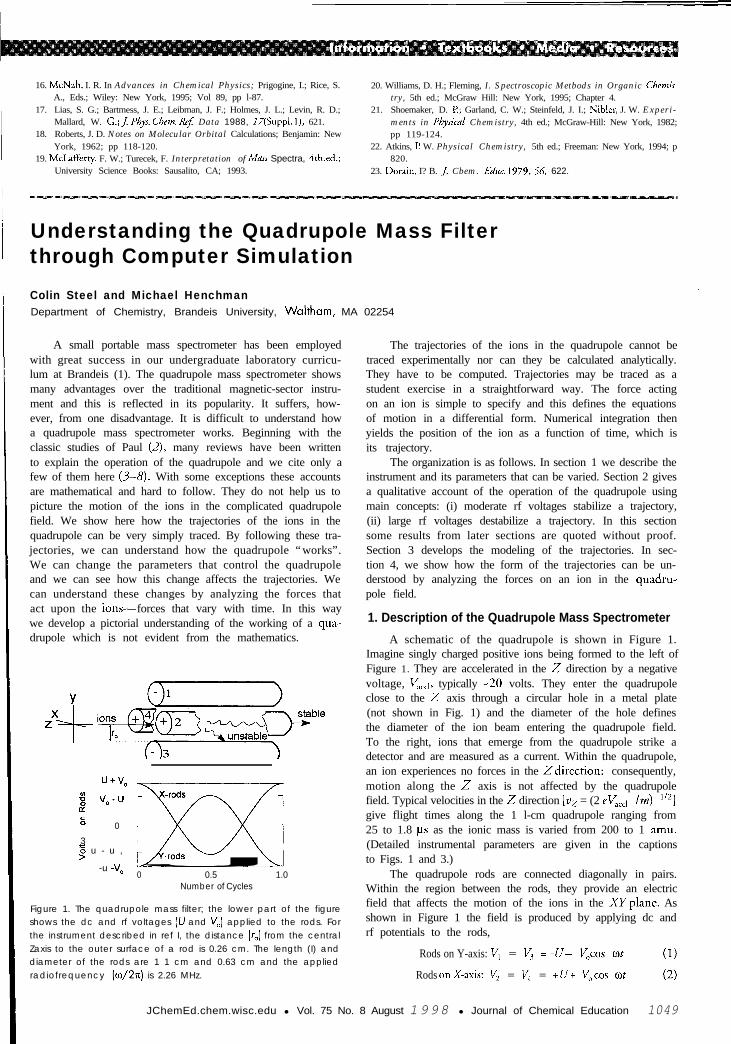
Figure 1. The quadrupole mass filter; the lower part of the figureshows the dc and rf voltages (U and V,) applied to the rods. Forthe instrument described in ref I, the distance (r-J from the centralZaxis to the outer surface of a rod is 0.26 cm. The length (I) anddiameter of the rods are 1 1 cm and 0.63 cm and the appliedradiofrequency (o/274 is 2.26 MHz.

The trajectories of the ions in the quadrupole cannot betraced experimentally nor can they be calculated analytically.They have to be computed. Trajectories may be traced as astudent exercise in a straightforward way. The force actingon an ion is simple to specify and this defines the equationsof motion in a differential form. Numerical integration thenyields the position of the ion as a function of time, which isits trajectory.

The organization is as follows. In section 1 we describe theinstrument and its parameters that can be varied. Section 2 givesa qualitative account of the operation of the quadrupole usingmain concepts: (i) moderate rf voltages stabilize a trajectory,(ii) large rf voltages destabilize a trajectory. In this sectionsome results from later sections are quoted without proof.Section 3 develops the modeling of the trajectories. In sec-tion 4, we show how the form of the trajectories can be un-derstood by analyzing the forces on an ion in the quadru-pole field.

1. Description of the Quadrupole Mass Spectrometer

A schematic of the quadrupole is shown in Figure 1.Imagine singly charged positive ions being formed to the left ofFigure 1. They are accelerated in the 2 direction by a negativevoltage, L&l, typically -20 volts. They enter the quadrupoleclose to the 2 axis through a circular hole in a metal plate(not shown in Fig. 1) and the diameter of the hole definesthe diameter of the ion beam entering the quadrupole field.To the right, ions that emerge from the quadrupole strike adetector and are measured as a current. Within the quadrupole,an ion experiences no forces in the Zdirection: consequently,motion along the 2 axis is not affected by the quadrupolefield. Typical velocities in the 2 direction [vz = (2 eV,,,1 lm) 1'2]give flight times along the 1 l-cm quadrupole ranging from25 to 1.8 I.LS as the ionic mass is varied from 200 to 1 amu.(Detailed instrumental parameters are given in the captionsto Figs. 1 and 3.)

The quadrupole rods are connected diagonally in pairs.Within the region between the rods, they provide an electricfield that affects the motion of the ions in the XYplane. Asshown in Figure 1 the field is produced by applying dc andrf potentials to the rods,

Rods on Y-axis: V, = V3 =-U- V,cos cotRods onX-axis: V2 = V, = +U+ V,cos cot

(1)(2)


where U is the dc potential and V, is the amplitude of the rfpotential, applied at a fixed frequency o/271: in the MHzrange. With a flight time of 25 ps, an ion experiences about50 rf cycles while traversing the quadrupole.

2. The Operation of the Quadrupole Mass SpectrometerThe working of a quadrupole mass spectrometer is com-

plicated and our aim here is to bring the reader to a simpleunderstanding. In section 2.1 we consider ions of a single massm entering a quadrupole and we ask which voltages, U andV,, let the ions be transmitted and which let them be deflected.We represent our findings on a plot of Uagainst V,, which isknown as a stability didgrdm (Fig. 2). Unfortunately such astability diagram only applies to ions of a particular mass.

In section 2.2 we develop the generalized stability didgram(Fig. 4)-much more useful because it applies to all masses.The generalized diagram has two important applications. Itreveals how the quadrupole can filter ions according to theirmass-to-charge ratio (2.2.1) and it reveals how the quadru-pole mass spectrometer can produce a mass spectrum (2.2.2).

In this section, we shall also examine the trajectories ofions in the quadrupole, obtained as described in section 3.The outcome of these trajectories-whether an ion is trans-mitted or deflected-enables us to draw the stability diagram.The detailed waveform of the trajectories (what the trajecto-ries of the ions actually look like for different settings of Uand V,) reveals how the quadrupole works.

2.7. Ions of a Single Mass: the Stability DiagramWe start with the simplest possible case, a quadrupole

with the radio frequency (0) fixed and ions of only one mass(m). Only two controls can be varied, the dc voltage (U) andthe rf amplitude (V,). There ore we ask: For what values offU and V, will the quadrupole transmit the ions, allowing themto strike the detector and be recorded as a current? For whatvalues will the ions be deflected, strike the rods, and be lost?To answer these questions, we could perform a large numberof experiments, varying U and V, and viewing the outcome(transmission or deflection). Our results would then be mostsimply expressed on a plot of U versus V, (Fig. 2). Eachexperiment would be represented by a single point on thisplot and in each case we would record the outcome. Ourexperiments would show that all ions with Uand V, valueslying within the “triangle” in Figure 2 are transmitted; thoselying outside the triangle are deflected to one of the rods.

Consider the points C and D in Figure 3. These pointslie within the stability triangle; their trajectories must be stable,and the ions must be transmitted. Figure 3 shows that the Xand Y trajectories are all stable, as they should be. To “read”these trajectories, recall that the quadrupole does not act onthe ion in the Zdirection but only in the XYplane; and motion

Figure 2 is called a stability diapam. For ions to be trans-mitted through the quadrupole, their trajectories must bestable. When ions are deflected to a rod, their trajectories areunstable. The region within the stability diagram in which alltrajectories are stable is roughly shaped like a triangle and maybe called the “stability triangle”. To understand the stabilitydiagram we must examine the shapes of the trajectories inthe various regions of the diagram. We obtain these trajectoriesby procedures developed in section 3. At this stage we cannotderive them but we can quote them and use them to under-stand the working of the quadrupole.

apex of stability region&

80

gP 70

. 80

= 50E!ka 4o2 30

x yil XandYstable \

Owl I I I I I\ I100 300

RF amplitude V, /5f&s700

Figure 2. The stability diagram for a particular ionic mass in termsof the applied dc voltage (u) and rf amplitude (V,). Xand Y direc-tions are defined in Figure 1 and are used throughout the text.

X-Axis Y-Axis

UKey:

Figure 3. X and Y trajectories for the points A, B, C, D, E in Figure2. Constant U (= 33 volts) and various V, (0, 305, 310, 585, 590volts). x0 = y0 = 0.07 cm, r, = 0.26 cm, L = 1 1 cm, m = 199 amu,o-) = 14.2 x 1 O6 rad/s. V,,,, = 20 V; time of flight through quadru-pole = 25 ps.

in the XYplane is traced most simply by two trajectories, onealong the Xaxis and one along the Y: In each of the 10 trajec-

We can now label the various regions of the stability

tory diagrams the upper and lower boundaries correspond torod surfaces. Since the velocity in the 2 direction is constant,

diagram as unstable or stable (Fig. 2). Trajectories are stable

the horizontal axis in each diagram represents both the length

within the stability triangle, requiring both the X and Y

of a rod and the time for an ion to traverse the filter.

trajectories to be stable (Fig. 3, C and D). Outside thestability triangle, trajectories are unstable. This could resultfrom instability of either the X trajectory or the Y trajectory.


Once agOutside 1unstableComplenof V,, theby Figure

FinalAt lower 1outside (1unstableity bounctrajectory+ E) andthe Xstat

Weaof the staroughly 1have a p(negative (jectories I(and ultilvoltages?understarinvoke tw

a. Lo

b. H i

Therod switclfirst attraceffects shein sectionthe ion to

The Ilarge osciand the iultimatelysection 4

Usin;of the stalC-+D+simple to ;

Pointwith the rexactly orwill repeldirection.[Xl). Rodpositive icrod is close[Y]). Notthe stabili

We nbut still 1~motion isthe YmolB, it has bflight timtrajectoryat C, just 5boundary.voltage nc

Once again, the trajectory calculations provide the answer.Outside the triangle, at lower values of V,, the Ytrajectory isunstable and the X is stable, as shown by Figure 3, A and B.Complementing this, outside the triangle, at higher valuesof Vo, the Xtrajectory is unstable and the Ystable, as shownby Figure 3, insert E.

Finally, we can label the boundaries of the stability triangle.At lower values of V,, moving inside the stability triangle fromoutside (Fig. 3, B 3 C), the Ytrajectory changes from beingunstable to stable and so the boundary is called the Ystabil-ity boundary. Likewise, for higher values of V,, it is the Xtrajectory which changes from stable to unstable (Fig. 3, D+ E) and the upper boundary of the stability triangle is calledthe Xstability boundary.

We ask the following general questions about the shapeof the stability diagram. Why is the stability region shapedroughly like a triangle? Why does the Y stability boundaryhave a positive slope and the X stability boundary a steepnegative one? Why are the Xtrajectories stable and the Ytra-jectories unstable at low rf voltages? Why do X trajectories(and ultimately Y trajectories) become unstable at high rfvoltages? Answers to these questions come from a qualitativeunderstanding of the stability diagram. To proceed, we mustinvoke two results developed in section 4:

a. Low rf voltages stabilize the trajectory; andb. High rf voltages destabilize the trajectory.

The first seems counterintuitive. As the rf voltage on arod switches from negative to positive, a positive ion will befirst attracted, then repelled. Intuition suggests that these twoeffects should cancel but actually they don’t. As we shall seein section 4 and from Figure 5, the overall effect is to drivethe ion towards the central Zaxis and stabilize the trajectory.

The second is simpler to grasp. Large rf voltages inducelarge oscillations in the motion of the ion about the 2 axisand the increasing amplitude in the motion causes the ionultimately to strike a rod. Again an analysis is given later insection 4 and displayed in Figure 6.

Using these two concepts, we now explore the featuresof the stability diagram by moving along the line A + B +C + D + E in Figures 2 and 3 (where Uis fixed). Point A issimple to analyze and we use a and b (above) to analyze the rest.

Point A represents the situation of an ion in a dc fieldwith the rf switched off. In general the ion will not be locatedexactly on the 2 axis. Rods 2 and 4, at a positive dc voltage,will repel the positive ion, causing it to oscillate in the Xdirection. X motion is therefore stable (Fig. 3, trajectory A[Xl). Rods 1 and 3, at a negative dc voltage, will attract thepositive ion, which will move toward and strike whicheverrod is closer. Ymotion is therefore unstable (Fig. 3, trajectory A[Y]). Note that the Xstability and Yinstability are shown inthe stability diagram (Fig. 2).

We now move A + B + C. The rf voltage is increasingbut still low, so that its action is stabilizing (a). At A, the Xmotion is stable; moving to C, it becomes more so. At A,the Y motion is unstable with the briefest of flight times; atB, it has been stabilized a little, still unstable but with a longerflight time; and at C, the stabilizing rf field has made thetrajectory stable. At B, the Ymotion is still just unstable andat C, just stable, with the switchover occurring at the Ystabilityboundary. The larger the initial dc voltage, the larger the rfvoltage needed to offset it. For that reason, the Y stability

boundary has a positive slope. Traces of the Xand Ytrajectoriesfor A, B, and C validate this description (Fig. 3).

We now move C + D + E. The rf voltage is still in-creasing but is now large, so that its action is destabilizing(6). At C, both Xand Y motions are stable: ultimately bothmust become unstable. The Xmotion becomes unstable at alower voltage (Fig. 3, trajectories E [X] and E[Y]). Again,traces of the X and Y trajectories for C, D, and E validatethis description (Fig. 3). The switchover from Xstable to Xunstable occurs at the Xstability boundary, which has a steepnegative slope (Fig. 2). In section 4 we shall find that in thecase of Xmotion, the dc potential (U) reinforces the large rfpotential (V,) in driving the ion towards the Xrods; hence asU increases the value of V, required to obtain X instabilitydecreases, resulting in a negative slope for the X stabilityboundary. The steepness of the slope is associated with thefact that the value at which the Xmotion becomes unstabledepends mainly on the large rf voltage (V,) and, to first approxi-mation, is independent of the relatively modest dc voltage.

The stability diagram describes the working of thequadrupole for ions of a single mass. We now generalize thedescription for ions of all masses in terms of the generalizedstability diagram. This involves only resealing the axes; theshape of the diagram remains unchanged.

2.2. Ions of A// Masses: the Generalized StabilityDiagram

For ions of a single mass, the stability diagram describesthe range of quadrupole settings, U and V,, which cause theion to be deflected or transmitted. For each different mass,there is a different stability diagram. We need one diagramthat will work for all masses. Theory (derived in section 3.1)tells us to replace the variables Uand V, by new variables aand 4, which we can think of as U/m and VJm. There areother terms in a and 4 (eqs 3 and 4) but they can be ignoredbecause they are constant.

When we make an a versus 4 plot, we obtain the gener-alized stability diagram (Fig. 4), which applies to all masses(strictly, all mass-to-charge ratios). Its universal applicability

A 6 CX- Axis

Y-axis -

m = 2020 . 2 5 r

..~.m= 199

J /

m= 197

I I I I

0.4 0 .6 0 .8 1 .oq = 4eVJmr,*0*

Figure 4. Generalized stability diagram in terms of the dimension-less parameters a and q. The three inset diagrams show X and Ytrajectories for m = 202, 199, and 197 amu in the regions exhib-iting (A) Y instability, (6) no instability, and (C) X instability. For allinsets lJ = 82 volts and V, = 497 volts, V,,,, = 20 volts, r, = 0.26cm,x,=y,=O.l cm,l=ll cm,o=14.2x106rad/s.

JChemEd.chem.wisc.edu Vol. 75 No. 8 August 1998 Journal of Chemical Education 1051

is shown by the location of the apex, which is always at the(a, 4) point (0.237, 0.706). Again the X stability boundaryalways terminates at the (a, 4) point (0, 0.91). Using thegeneralized stability diagram it is easy to show how the quadru-pole works as a mass-to-charge ratio filter and how it candeliver a mass spectrum.

2.2.1. The Quadrupole as a Mass Filter

Again we restrict discussion to singly charged ions. Fora quadrupole to function as a mass filter with unit mass reso-lution, it must be able to separate mass m from mass (m - 1)and lower masses, and from mass (m + 1) and higher masses.That is, we have to be able to tune the quadrupole so thatmass m lies within the stability triangle, whereas all othermasses, (m - 1) and lower and (m + 1) and higher, do not.How can we do this? We could tune mass m to the tip of theapex of the generalized stability diagram (Fig. 4) because mostof the surrounding points lie outside the stability diagram.In principle, that is a good idea; in practice it isn’t, becauserandom voltage fluctuations in U and V, would move themass m in and out of the stability triangle. In practice we tuneit not to the apex (a = 0.237; q = 0.706) but slightly below,say to point B in Figure 4 (a = 0.233; q = 0.706), wherenoise will not kick the ion of mass m out of the triangle.

With the quadrupole tuning mass m to the point B (Fig.4), we now check on masses (m - 1) and (m + 1). If they lieoutside the stability triangle, the quadrupole can act as a massfilter. If they lie inside, mass m will not be selected frommasses (m- 1) and (m + 1).

We start by calculating the quadrupole voltages neededto focus the mass m on the point B. We call these values Uand V,. By using the equations that define a and q (section3) and substituting the values of a and q that define the pointB, we can evaluate Uand V,,

a = 8eUlmr ‘a2 = 0.2330 (3)q = 4 e VJm ro2 o2 = 0.706 (4)

We now ask, with the quadrupole tuned at voltages Uand V,, where the (singly charged) masses (m - 1) and (m +1) will appear on the stability diagram.

Let’s start with mass (m - 1). We want to locate its posi-tion on Figure 4 (i.e., its a and q values). These are given byeqs 5 and 6:

a = 8 eU/(m - l)ro202 (5)q = 4 eV,/(m - 1) ro202 (6)

Notice that the a and q values for mass (m - 1) are both largerby the same factor, m/(m - l), than those for mass m at pointB. Since the ratio (a/q) is fixed (by the tuning of m to B), mass(m - 1) will be located on the straight line drawn throughthe origin and passing through B.. . somewhere in the vicinityof point C. The corresponding values for mass (m + 1) willbe smaller, placing it on the same straight line but now belowB . . . somewhere in the vicinity of point A. The straight lineon which these masses lie is called the scan line. Clearly, forgiven values of Uand V, all masses lie on the same scan line.

To investigate if a particular quadrupole can function asa mass filter in a particular case, we must establish whetherpoints A and C lie inside or outside the stability triangle. Insection 3 we use the trajectories shown in Figure 4 to estab-lish the resolution that can be achieved.

2.2.2. Running a Mass Spectrum on the QuadrupoleThe above discussion tells us that to maximize resolu-

tion, each mass must progressively be brought to point B inFigure 4. When any particular mass is being measured, allthe other masses will be strung out along the scan line, theheaviest closest to and the lightest furthest from the origin.To run a mass spectrum, we move all the masses progres-sively through point B. This is done by starting at a low valuefor U and V, and progressively increasing both while keep-ing the ratio U/V, constant at ‘/,(0.233/0.706) throughout.

3. Computer Modeling

In this section we show how the performance of the quadru-pole may be analyzed under any conditions by examiningthe trajectories of the ions, which are readily obtained bycomputer simulation. The first step is to derive the equationsgoverning the motion of the ions. Although these equationsmay be found in other references (2-5, Z S), they are repeatedhere for convenience and completeness.

3.7. Theoretical BackgroundThe dc and rf voltages determine the potential in the

X-Y plane in the charge-free region between the rods andthe potential (V) there must satisfy the two-dimensionalLaplace equation (7, 10) d2%‘/Jg + a22//Jy = 0. The simplestequation satisfying this differential equation is, V(x,y) =(x2 - y”) *K where K is some constant determined by theboundary conditions. The internal surfaces of the rods markthe edge of the charge-free region and fix the boundary con-ditions on the X and Y axes so that

v((-r,,O) = z/(r,,O) = (U+ V, cos ot)and

V (0, -r,) = (I/ (0, r,) = -(U + V, cos ot)

so that K = (U + V, cos ot)/ro2. Thus,

V (x,y) = (2 -y’)( U + V, cos ot)/ro2 (7)We see from eq 7 that an equipotential curve within thequadrupole, that is, V(x,y) = const, has the form of a rectan-gular hyperbola. Indeed, early quadrupoles were constructedusing rods having hyperbolic surfaces (2, 6). But in practicethis was found to be unnecessary, and rods circular in cross-section, which are much more easily fabricated, are now used.

The force in the Xdirection on an ion, charge e, at (x,r>is F’ = -e 3%’ /ax, with a similar formula for the force FJ in theY direction. These equations for F, and P? in conjunctionwith Newton’s second law (force = mass . acceleration) andeq 7 immediately yield

F, = m *d 2xldt2 = -2e( U + V, cos 03 t) xlro2 (8)FY = m*d2y/dt2 = 2e( U + V, cos wt)y/r,= (9)

Notice that, since there are no cross terms, the motions in the Xand Y directions are independent. This justifies displayingion trajectories as independent X and Y paths in Figures 3 and4. Equations 8 and 9 are second-order differential equations.Generally they are recast (4) into dimensionless form by usingthe substitutions

ql = otl2 (10)a = 8eU/r,2m02 (3’)q = 4eV,/r,2m02 (4’)


in which c$

The paran-again that I

to-charge rFinal11

a2v/ax= + (for the quasimilar the1

3.2. Trajef

To gerferential ecto providepossible: irintegrationfirst recastand ZJ = dy/

d

6

Numestarts at angenerates atimes. Theset (xi, yi, t,tions abouassume thapole off axyo, t,> to (usuch that iestimated su,dt; dyO =are given twhich wasthe numerica factor ofupper limiiion througvalue of vz

Usingprogram tatrajectoriesexperiment

This aa quadrupc

1. For 1thatthe IwellmuI:is theI’me 1estlywheldropnewtorieis incao.70

in which case they become

d2x/d+2 = -(a + 2q cos 2@)x 03’)d2yldQ2 = (a + 2q cos 241)~ (9’)

The parametric dependence of a and q on m/e emphasizesagain that the quadrupole sorts ions according to their mass-to-charge ratio.

Finally, the equivalent three-dimensional Laplace equationa2v l&G + a2’11 /a~? + a22/ /&? = 0 is the fundamental equationfor the quadrupole storage ion trap (2, 5, 7) and an essentiallysimilar theory applies to these devices.

3.2. Trajectory GenerationTo generate ion trajectories, we have to integrate the dif-

ferential equations of motion (8 and 9). Direct integrationto provide analytical solutions for the ion trajectories is notpossible: instead, they are derived very easily by numericalintegration, using a few lines of computer code. To do so wefirst recast eqs 8 and 9 in first-order form, defining u = dxldtand v = dyldt as the velocities in the Xand Ydirections:

duldt = -2e( U+ V, cos at) xlmro2 = f (t,x) (11)dvldt = 2e(U + V, cos ot)ylmro2 = g(t,y) (12)

Numerical integration by the Euler method (II, 12)starts at an initial state (uO, uO, x0, yO, to). A time interval d tgenerates a new state (ul, ul, x1, yl, tl). This is repeated ntimes. The trajectory of the ion is then represented by theset (xi, yj, tj), where i = 0, 1, . . ., n. We have to make assump-tions about the initial conditions. At time zero (to = 0) weassume that u, = v, = 0 and that the ion enters the quadru-pole off axis at the point (x0, y,J. In passing from (z+,, vO, x0,yo, to> to (u,, q, x1, yl, tJ, changes duo, duo, dq,, dy,, 4, occursuch that u1 = u, + du,, etc. The incremental changes areestimated as follows: du, = f (to, x,)dt; dv, = g(t,, yJdt; dxo =u,dt; dye = v,dt; dto = dt. Better estimates of these incrementsare given by the 4th-order Runge-Kutta method (II, 12),which was employed throughout this study in implementingthe numerical integration. The time interval (dt) was typicallya factor of 30 less than the period (2nlco) of the rf field. Theupper limit of integration is given by the flight time of theion through the quadrupole, which is determined from thevalue of vz and L.

Using a 486 PC and uncompiled QuickBasic, such aprogram takes less than two seconds to run and display thetrajectories on the monitor, so a student can quickly changeexperimental parameters and view the results.

This allows for ready experimentation to examine howa quadrupole “works”:

1. For the conditions shown in Figure 4 the mass rangethat gets through the filter is about 199 + 2.25, so thatthe resolution is mlbm = 19912.25 = 88. This agreeswell with the value obtained from the empirical for-mula (5) m/Am = 0.357/(0.237 - CJ,,,,~), where aO.706is the value of a at the point of intersection of the scanline with q = 0.706. Lowering a/q (or UI V,) even mod-estly can result in a serious loss of resolution. Thus,when a/q is lowered by 10% to 0.30 the resolutiondrops to = 12. By changing Uand V, so as to tune in anew mass to point B (Fig. 4) and tracing new trajec-tories, the student can show that the resolution m/Amis independent of m and depends only on the value ofa0.706.

2. In Figure 3 we showed how for a given mass and atconstant dc potential (U) the points on the Y and Xstability boundaries could be obtained by systemati-cally increasing V, and looking at the values of V, atwhich the changes from Yunstable to Ystable and fromXstable to Xunstable occur. By varying Uand repeatingthis procedure the stability diagram may be mapped.

3. Other factors that can influence the resolving power of aquadrupole (5), such as o), the initial values x,,y,,, the rodlength L, and the rod separation (2 r,) are quite subtleand require a more detailed analysis, accounting forthe fact that not all ions will start with U, = v, = 0.

4. Detailed Description of the Trajectories

In this section, a closer examination of the forces on anion and the resulting trajectories elucidates and clarifies themain concepts used in section 2: (i) moderate rf voltages arestabilizing, and (ii) large rf voltages are destabilizing.

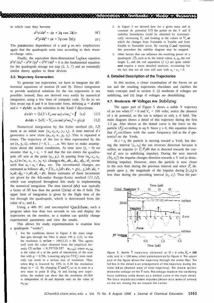
4.7. Moderate RF Vohuges Are SkddizingThe upper part of Figure 5 shows a stable Y trajectory

of an ion when U = 0 and V, = 100 volts; notice the absenceof a dc potential, so the ion is subject to only a rf field. Themain diagram shows a detail of this trajectory during the first1.5 ps. Also shown as the dotted curve is the force on theparticle (FJ according to eq 9. Since y > 0, this equation showsthat F oscillates with the same frequency (0) as the rf po-tentia r’on the Yrods.

At t = t, the particle is moving toward a Yrod, but dur-ing the interval [tl, t2] the ion reverses direction because itsuffers an impulse (= QFJ,dt) that is directed towards the cen-tral 2 axis (a stabilizing impulse). During the next interval( [t2, t3]) the impulse changes direction towards a Y rod (a desta-bilizing impulse). However, since the particle is now closerto the axis than during the previous interval and since Fy de-pends upon y, the magnitude of the impulse during [t2,t3] isless than during the preceding interval [tl , t2]. Thus the par-

Time (ps)Total Traiectory 5 10 15 20

Detail rod face

Z axis

“.,. Force: . . .‘._,

:I I rod faceI

/‘-.RFVoltaae .r.\I.-’

- - - 1.1 L-d./0 0.5 1.0

Time (ps)1.5

Figure 5. Stable Y trajectory obtained at U = 0 volts, V, = 100volts, and m = 199 amu; other parameters as for Figure 4. The upperpart of the figure shows the trajectory through the entire filter. Thefull line in the detail is an enlargement of this trajectory during theinitial 1.5 ps (shaded area of total trajectory). The lowest sectionshows the voltage on the Y rods. This voltage results in the oscillatingforce (arbitrary units) shown as a dotted curve in the main detail.The force imparts successive impulses (shown as a series of arrows)on the ion, driving the ion toward the center.


Time (~1s)

/ I I / rod faceIRF Voltaqe

II.>.& 1 cycle -.I

‘\.-.I.I ‘\.-/ 1 1

2.6 2.8 3.0 3.2Time (ps)

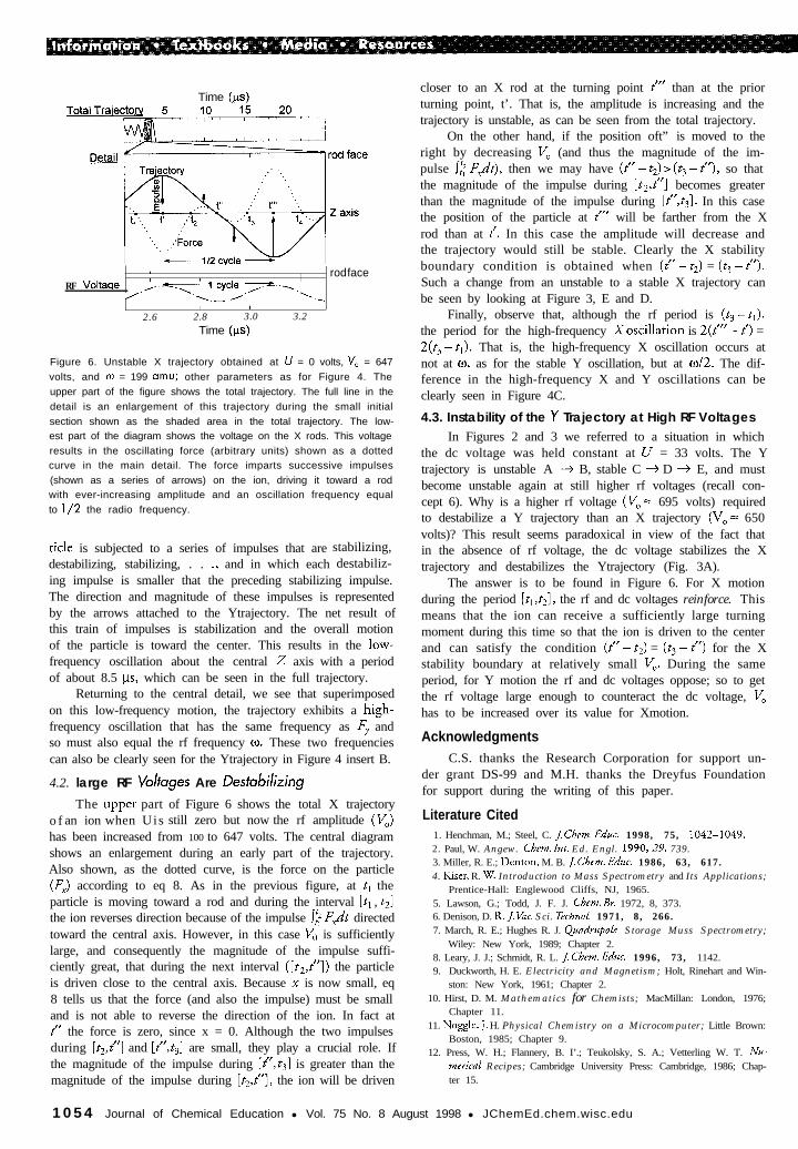
Figure 6. Unstable X trajectory obtained at U = 0 volts, V, = 647volts, and m = 199 amu; other parameters as for Figure 4. Theupper part of the figure shows the total trajectory. The full line in thedetail is an enlargement of this trajectory during the small initialsection shown as the shaded area in the total trajectory. The low-est part of the diagram shows the voltage on the X rods. This voltageresults in the oscillating force (arbitrary units) shown as a dottedcurve in the main detail. The force imparts successive impulses(shown as a series of arrows) on the ion, driving it toward a rodwith ever-increasing amplitude and an oscillation frequency equalto l/2 the radio frequency.

title is subjected to a series of impulses that are stabilizing,destabilizing, stabilizing, . . ., and in which each destabiliz-ing impulse is smaller that the preceding stabilizing impulse.The direction and magnitude of these impulses is representedby the arrows attached to the Ytrajectory. The net result ofthis train of impulses is stabilization and the overall motionof the particle is toward the center. This results in the low-frequency oscillation about the central 2 axis with a periodof about 8.5 ps, which can be seen in the full trajectory.

Returning to the central detail, we see that superimposedon this low-frequency motion, the trajectory exhibits a high-frequency oscillation that has the same frequency as Fy andso must also equal the rf frequency ci). These two frequenciescan also be clearly seen for the Ytrajectory in Figure 4 insert B.

4.2. large RF Vohages Are Destcddizing

o fThe upper part of Figure 6 shows the total X trajectory

an ion when Uis still zero but now the rf amplitude (V,)has been increased from 100 to 647 volts. The central diagramshows an enlargement during an early part of the trajectory.Also shown, as the dotted curve, is the force on the particle(F,) according to eq 8. As in the previous figure, at tl theparticle is moving toward a rod and during the interval [t, , tJthe ion reverses direction because of the impulse 1: F,dt directedtoward the central axis. However, in this case V, is sufficientlylarge, and consequently the magnitude of the impulse suffi-ciently great, that during the next interval ([tJ’]) the particleis driven close to the central axis. Because x is now small, eq8 tells us that the force (and also the impulse) must be smalland is not able to reverse the direction of the ion. In fact att” the force is zero, since x = 0. Although the two impulsesduring [t2,tl’] and [tl’,tJ are small, they play a crucial role. Ifthe magnitude of the impulse during [fl,tg] is greater than themagnitude of the impulse during [t.,t”], the ion will be driven

closer to an X rod at the turning point t”’ than at the priorturning point, t’. That is, the amplitude is increasing and thetrajectory is unstable, as can be seen from the total trajectory.

On the other hand, if the position oft” is moved to theright by decreasing V, (and thus the magnitude of the im-pulse J; F,dt), then we may have (t” - tZ) > (t3 - t”), so thatthe magnitude of the impulse during [t+“] becomes greaterthan the magnitude of the impulse during [P’,tJ. In this casethe position of the particle at t”’ will be farther from the Xrod than at t’. In this case the amplitude will decrease andthe trajectory would still be stable. Clearly the X stabilityboundary condition is obtained when (t” - tz) = (t3 - t”).Such a change from an unstable to a stable X trajectory canbe seen by looking at Figure 3, E and D.

Finally, observe that, although the rf period is (t3 - ti),the period for the high-frequency Xoscillation is 2(t”’ - t’) =2(t3 - ti). That is, the high-frequency X oscillation occurs atnot at ci), as for the stable Y oscillation, but at CO/~. The dif-ference in the high-frequency X and Y oscillations can beclearly seen in Figure 4C.

4.3. Instability of the Y Trajectory at High RF VoltagesIn Figures 2 and 3 we referred to a situation in which

the dc voltage was held constant at U = 33 volts. The Ytrajectory is unstable A 3 B, stable C + D 3 E, and mustbecome unstable again at still higher rf voltages (recall con-cept 6). Why is a higher rf voltage (V, = 695 volts) requiredto destabilize a Y trajectory than an X trajectory (V, = 650volts)? This result seems paradoxical in view of the fact thatin the absence of rf voltage, the dc voltage stabilizes the Xtrajectory and destabilizes the Ytrajectory (Fig. 3A).

The answer is to be found in Figure 6. For X motionduring the period [ti,tJ, the rf and dc voltages reinforce. Thismeans that the ion can receive a sufficiently large turningmoment during this time so that the ion is driven to the centerand can satisfy the condition (t” - tZ) = (t3 - t”) for the Xstability boundary at relatively small V,. During the sameperiod, for Y motion the rf and dc voltages oppose; so to getthe rf voltage large enough to counteract the dc voltage, V,has to be increased over its value for Xmotion.

AcknowledgmentsC.S. thanks the Research Corporation for support un-

der grant DS-99 and M.H. thanks the Dreyfus Foundationfor support during the writing of this paper.

Literature Cited1. Henchman, M.; Steel, C. J Chem. Educ. 1998, 75, 1042-1049.2. Paul, W. Angew. Chem. ht. Ed. Engl. 1990,29, 739.3. Miller, R. E.; Denton, M. B. J Cbem. Educ. 1986, 63, 617.4. Kiser, R. W. Introduction to Mass Spectrometry and Its Applications;

Prentice-Hall: Englewood Cliffs, NJ, 1965.5. Lawson, G.; Todd, J. F. J. Chem. Br. 1972, 8, 373.6. Denison, D. R.j. Vat. Sci. Technol. 1971, 8, 266.7. March, R. E.; Hughes R. J. Quadrupole Storage Muss Spectrometry;

Wiley: New York, 1989; Chapter 2.8. Leary, J. J.; Schmidt, R. L. J Gem. Educ. 1996, 73, 1142.9. Duckworth, H. E. Electricity and Magnetism; Holt, Rinehart and Win-

ston: New York, 1961; Chapter 2.10. Hirst, D. M. Mathematics for Chemists; MacMillan: London, 1976;

Chapter 11.11. No&e, J. H. Physical Chemistry on a Microcomputer; Little Brown:

Boston, 1985; Chapter 9.12. Press, W. H.; Flannery, B. I’.; Teukolsky, S. A.; Vetterling W. T. Nu-

merical Recipes; Cambridge University Press: Cambridge, 1986; Chap-ter 15.


Techn

Abstra

Lois M. BDepartmen

This isistry, a cornthe basic tgraduate UIBrowne anUniversity (a unique siThe set is csteps of batvisually inn

Part 2videotape tsegments d,

. reflu:

. using

. simp

. reduc

. using

Part 1,viously (3).

In Teclthe basic m;ment is pretants introdlying fundais detailed 1

design and operation of a portable quadrupole mass spectrometer for the undergraduate

Documents