design and optimization of membrane-type acoustic

University of Nebraska - LincolnDigitalCommons@University of Nebraska - LincolnArchitectural Engineering -- Dissertations andStudent Research Architectural Engineering

5-2016

Design and Optimization of Membrane-TypeAcoustic MetamaterialsMatthew G. BlevinsUniversity of Nebraska-Lincoln, [email protected]

Follow this and additional works at: http://digitalcommons.unl.edu/archengdiss

Part of the Acoustics, Dynamics, and Controls Commons, and the Architectural EngineeringCommons

This Article is brought to you for free and open access by the Architectural Engineering at DigitalCommons@University of Nebraska - Lincoln. It hasbeen accepted for inclusion in Architectural Engineering -- Dissertations and Student Research by an authorized administrator ofDigitalCommons@University of Nebraska - Lincoln.

Blevins, Matthew G., "Design and Optimization of Membrane-Type Acoustic Metamaterials" (2016). Architectural Engineering --Dissertations and Student Research. 38.http://digitalcommons.unl.edu/archengdiss/38

http://digitalcommons.unl.edu?utm_source=digitalcommons.unl.edu%2Farchengdiss%2F38&utm_medium=PDF&utm_campaign=PDFCoverPages

http://digitalcommons.unl.edu/archengdiss?utm_source=digitalcommons.unl.edu%2Farchengdiss%2F38&utm_medium=PDF&utm_campaign=PDFCoverPages


http://digitalcommons.unl.edu/architectengineer?utm_source=digitalcommons.unl.edu%2Farchengdiss%2F38&utm_medium=PDF&utm_campaign=PDFCoverPages


http://network.bepress.com/hgg/discipline/294?utm_source=digitalcommons.unl.edu%2Farchengdiss%2F38&utm_medium=PDF&utm_campaign=PDFCoverPages



http://digitalcommons.unl.edu/archengdiss/38?utm_source=digitalcommons.unl.edu%2Farchengdiss%2F38&utm_medium=PDF&utm_campaign=PDFCoverPages

DESIGN AND OPTIMIZATION OF MEMBRANE-TYPE

ACOUSTIC METAMATERIALS

by

Matthew Grant Blevins

A DISSERTATION

Presented to the Faculty of

The Graduate College at the University of Nebraska

In Partial Fulfillment of Requirements

For the Degree of Doctor of Philosophy

Major: Architectural Engineering

Under the Supervision of Professor Lily M. Wang

Lincoln, Nebraska

May, 2016

DESIGN AND OPTIMIZATION OF MEMBRANE-TYPE

ACOUSTIC METAMATERIALS

Matthew Grant Blevins, Ph.D.

University of Nebraska, 2016

Advisor: Lily M. Wang

One of the most common problems in noise control is the

attenuation of low frequency noise. Typical solutions require barriers

with high density and/or thickness. Membrane-type acoustic

metamaterials are a novel type of engineered material capable of high

low-frequency transmission loss despite their small thickness and light

weight. These materials are ideally suited to applications with strict

size and weight limitations such as aircraft, automobiles, and

buildings. The transmission loss profile can be manipulated by

changing the micro-level substructure, stacking multiple unit cells, or

by creating multi-celled arrays. To date, analysis has focused

primarily on experimental studies in plane-wave tubes and numerical

modeling using finite element methods. These methods are inefficient

when used for applications that require iterative changes to the

structure of the material. To facilitate design and optimization of

membrane-type acoustic metamaterials, computationally efficient

dynamic models based on the impedance-mobility approach are

proposed. Models of a single unit cell in a waveguide and in a baffle, a

double layer of unit cells in a waveguide, and an array of unit cells in

a baffle are studied. The accuracy of the models and the validity of

assumptions used are verified using a finite element method. The

remarkable computational efficiency of the impedance-mobility models

compared to finite element methods enables implementation in design

tools based on a graphical user interface and in optimization schemes.

Genetic algorithms are used to optimize the unit cell design for a

variety of noise reduction goals, including maximizing transmission

loss for broadband, narrow-band, and tonal noise sources. The tools

for design and optimization created in this work will enable rapid

implementation of membrane-type acoustic metamaterials to solve

real-world noise control problems.

iv

Copyright 2016, Matthew G. Blevins

v

Acknowledgments

I would like to acknowledge several people without whom this research would not be

possible. First, I would like to thank Dr. Siu-Kit Lau for his idea of applying the

impedance-mobility approach to membrane-type acoustic metamaterials which

formed the basis of this research. His kindness as a person and diligence as a

researcher have greatly influenced my approach to learning. I would also like to

thank Dr. Lily Wang for advising me throughout my graduate career. Her

encouragement and support have been tremendously important to me. I would like

to thank Dr. Christos Argyropoulos and Dr. Christina Naify for their assistance

with finite element modeling. Thanks to Dr. Douglas Keefe and Caleb Sieck for

their conversations and pointed questions about my research. I would like to thank

the remaining members of my supervisory committee: Dr. Mahboub Baccouch, Dr.

Yaoqing Yang, and Dr. Erica Ryherd for their support and valuable feedback. I

would like to thank members of the Nebraska Acoustics Group for their friendship

and support throughout my career at UNL. Special thanks go to Christopher

Ainley, Andrew Hathaway, Ellen Peng, Hyun Hong, Joonhee Lee, and Laura Brill.

Lastly, I would like to thank my family; my parents, William and Jane Blevins, my

brother, William, and his wife, Sara, for their love, support, and encouragement.

Table of Contents

List of Figures x

List of Tables xix

1 Introduction and Literature Review 1

1.1 Motivation . . . . . . . . . . . . . . . . . . . . . . . . . . . . . . . . . 2

1.2 Research Objectives . . . . . . . . . . . . . . . . . . . . . . . . . . . . 6

1.3 Background . . . . . . . . . . . . . . . . . . . . . . . . . . . . . . . . 7

1.3.1 Metamaterials . . . . . . . . . . . . . . . . . . . . . . . . . . . 8

1.3.2 Impedance-Mobility Modeling . . . . . . . . . . . . . . . . . . 18

1.3.3 Genetic Algorithms . . . . . . . . . . . . . . . . . . . . . . . . 22

1.4 Dissertation Structure . . . . . . . . . . . . . . . . . . . . . . . . . . 29

2 Impedance-Mobility Modeling 31

2.1 Unit Cell . . . . . . . . . . . . . . . . . . . . . . . . . . . . . . . . . . 32

2.1.1 Baffled Transmission Loss . . . . . . . . . . . . . . . . . . . . 36

2.1.2 Membrane Stiffness . . . . . . . . . . . . . . . . . . . . . . . . 37

2.2 Cell Array . . . . . . . . . . . . . . . . . . . . . . . . . . . . . . . . . 39

2.2.1 2 x 1 Array . . . . . . . . . . . . . . . . . . . . . . . . . . . . 43

2.2.2 Negligible Coupling Model . . . . . . . . . . . . . . . . . . . . 45

2.3 Two Layers . . . . . . . . . . . . . . . . . . . . . . . . . . . . . . . . 46

2.4 Derived Quantities . . . . . . . . . . . . . . . . . . . . . . . . . . . . 51

2.4.1 Effective Dynamic Mass . . . . . . . . . . . . . . . . . . . . . 52

2.4.2 Reflection and Absorption Coefficients . . . . . . . . . . . . . 52

2.4.3 Panel Kinetic Energy . . . . . . . . . . . . . . . . . . . . . . . 53

2.4.4 Cavity Potential Energy . . . . . . . . . . . . . . . . . . . . . 54

2.5 Concluding Remarks . . . . . . . . . . . . . . . . . . . . . . . . . . . 54

3 Finite Element Verification 56

3.1 Verification of Accuracy . . . . . . . . . . . . . . . . . . . . . . . . . 57

3.1.1 Unit Cell in a Waveguide . . . . . . . . . . . . . . . . . . . . . 57

3.1.2 Unit Cell in a Baffle . . . . . . . . . . . . . . . . . . . . . . . 60

3.1.3 2×1 Array in a Baffle . . . . . . . . . . . . . . . . . . . . . . . 62

3.1.4 2×2 Array in a Baffle . . . . . . . . . . . . . . . . . . . . . . . 63

3.1.5 Double Layer in a Waveguide . . . . . . . . . . . . . . . . . . 65

3.2 Validation of Assumptions . . . . . . . . . . . . . . . . . . . . . . . . 66

3.2.1 Attached Mass Bending Stiffness . . . . . . . . . . . . . . . . 67

3.2.2 Attached Mass Rotary Inertia . . . . . . . . . . . . . . . . . . 70

3.2.3 Coupling Between Unit cells in an Array . . . . . . . . . . . . 73

3.3 Generalization to Other Unit Cell Geometries . . . . . . . . . . . . . 74

3.3.1 Circular Unit cell . . . . . . . . . . . . . . . . . . . . . . . . . 75

3.3.2 Hexagonal Unit Cell . . . . . . . . . . . . . . . . . . . . . . . 78

3.3.3 Triangular Unit Cell . . . . . . . . . . . . . . . . . . . . . . . 80

3.3.4 Remarks on Generalization to Other Unit Cell Geometries . . 83

3.4 Computational Efficiency . . . . . . . . . . . . . . . . . . . . . . . . . 84


4 Optimization Using Genetic Algorithms 89

4.1 Design Variables . . . . . . . . . . . . . . . . . . . . . . . . . . . . . 90

4.2 The Population . . . . . . . . . . . . . . . . . . . . . . . . . . . . . . 92

4.3 Fitness Functions . . . . . . . . . . . . . . . . . . . . . . . . . . . . . 93

4.3.1 Broadband . . . . . . . . . . . . . . . . . . . . . . . . . . . . 94

4.3.2 Narrow Band . . . . . . . . . . . . . . . . . . . . . . . . . . . 95

4.3.3 Discrete Frequency . . . . . . . . . . . . . . . . . . . . . . . . 97

4.3.4 Multiple Discrete Frequencies . . . . . . . . . . . . . . . . . . 98

4.3.5 Mass Law . . . . . . . . . . . . . . . . . . . . . . . . . . . . . 99

4.4 Selection, Crossover, and Mutation . . . . . . . . . . . . . . . . . . . 101

4.5 Convergence . . . . . . . . . . . . . . . . . . . . . . . . . . . . . . . . 103


5 Results 106

5.1 Impedance-Mobility Model . . . . . . . . . . . . . . . . . . . . . . . . 107

5.1.1 Single Unit Cell . . . . . . . . . . . . . . . . . . . . . . . . . . 107

5.1.2 Stacked Unit Cells . . . . . . . . . . . . . . . . . . . . . . . . 118

5.1.3 Multi-Cell Arrays . . . . . . . . . . . . . . . . . . . . . . . . . 123

5.1.4 Mass Law . . . . . . . . . . . . . . . . . . . . . . . . . . . . . 127

5.1.5 Derived Quantities . . . . . . . . . . . . . . . . . . . . . . . . 128

5.2 Genetic Algorithm Optimization . . . . . . . . . . . . . . . . . . . . . 134

5.2.1 Broadband . . . . . . . . . . . . . . . . . . . . . . . . . . . . 135

5.2.2 Octave Band . . . . . . . . . . . . . . . . . . . . . . . . . . . 138

5.2.3 Discrete Frequency . . . . . . . . . . . . . . . . . . . . . . . . 141

5.2.4 Multiple Discrete Frequencies . . . . . . . . . . . . . . . . . . 143


6 Conclusion and Recommendations for Future Work 148

6.1 Conclusion . . . . . . . . . . . . . . . . . . . . . . . . . . . . . . . . . 148

6.2 Recommendations for Future Work . . . . . . . . . . . . . . . . . . . 151

Bibliography 163

A Modes and Modal Radiation Efficiencies 164

B Tables 172

C Genetic Algorithm Optimal Results Tables 177

D Figures 184

E Application of Boundary Conditions 187

x

List of Figures

1.1 Schematic of 1-D metamaterial . . . . . . . . . . . . . . . . . . . . . 11

1.2 Cross-section of “Sonic Crystal” locally resonant acoustic metamaterial 12

1.3 Schematic of rectangular unit cell . . . . . . . . . . . . . . . . . . . . 14

1.4 Schematic of circular unit cell . . . . . . . . . . . . . . . . . . . . . . 14

1.5 Flowchart of a basic genetic algorithm . . . . . . . . . . . . . . . . . 24

1.6 Example of single point crossover and mutation . . . . . . . . . . . . 27

2.1 Schematic of rectangular unit cell . . . . . . . . . . . . . . . . . . . . 32

2.2 3x4 array of unit cells in a rigid baffle . . . . . . . . . . . . . . . . . . 39

2.3 Cross-section of two stacked unit cells . . . . . . . . . . . . . . . . . . 47

3.1 Unit cell in a waveguide FEM model A.) geometry, B.) mesh, and C.)

closeup of swept mesh . . . . . . . . . . . . . . . . . . . . . . . . . . 58

3.2 FEM verification of a single unit cell in a waveguide. Impedance-

mobility (solid), FEM (dashed) . . . . . . . . . . . . . . . . . . . . . 59

3.3 Baffled unit cell FEM model A.) geometry, and B.) mesh. . . . . . . . 61

xi

3.4 FEM verification of a single unit cell in a baffle. Impedance-mobility

(solid), FEM (dashed) . . . . . . . . . . . . . . . . . . . . . . . . . . 61

3.5 FEM geometry of baffled multi-cell arrays A.) 2×1 B.) 2×2 . . . . . . 62

3.6 FEM verification of a 2×1 array in a baffle. Impedance-mobility (solid),

FEM (dashed) . . . . . . . . . . . . . . . . . . . . . . . . . . . . . . . 63

3.7 FEM verification of a 2×1 array in a baffle. Impedance-mobility with

negligible coupling assumption (solid), FEM (dashed) . . . . . . . . . 64

3.8 FEM verification of a 2×2 array in a baffle using negligible coupling

model. Impedance-mobility (solid), FEM (dashed) . . . . . . . . . . . 64

3.9 Double layer in a waveguide FEM A.) geometry and B.) mesh. . . . . 65

3.10 FEM verification of a double unit cell in a waveguide. Impedance-


3.11 Cross-sections of A.) a 3D unit cell, B.) a simplified 3D unit cell and,

C.) an idealized 2D shell unit cell for use in FEM studies on the effect

of bending stiffness . . . . . . . . . . . . . . . . . . . . . . . . . . . . 68

3.12 FEM verification of a simplified 3D unit cell in a waveguide. Impedance-


3.13 FEM shell model verification of a single unit cell in a waveguide.

Impedance-mobility (solid), FEM (dashed) . . . . . . . . . . . . . . . 70

3.14 Comparison of impedance-mobility (solid) and FEM (dashed) trans-

mission loss of a unit cell with an eccentric mass location . . . . . . . 71

3.15 Example of rotary inertia of the attached mass at 460 Hz from FEM

model . . . . . . . . . . . . . . . . . . . . . . . . . . . . . . . . . . . 72

xii

3.16 Comparison of impedance-mobility (solid) and FEM (dashed) trans-

mission loss of a unit cell with a reduced thickness eccentrically placed

attached mass . . . . . . . . . . . . . . . . . . . . . . . . . . . . . . . 73

3.17 Example of rotary inertia of the attached mass at 790 Hz . . . . . . . 73

3.18 Surface pressure of a 2×1 array of unit cells in a baffle . . . . . . . . 74

3.19 Displacement of a 2×1 array of unit cells in a baffle . . . . . . . . . . 75

3.20 Comparison of TL from impedance-mobility model of a square unit cell

(solid) and FEM of a 3D circular unit cell (dashed) and 2D circular

unit cell (dotted) . . . . . . . . . . . . . . . . . . . . . . . . . . . . . 76

3.21 Geometry of 2D axial-symmetric FEM model . . . . . . . . . . . . . 77

3.22 Comparison of TL from impedance-mobility of a square unit cell (solid)

and FEM model of a circular unit cell (dashed) with an eccentric mass

location . . . . . . . . . . . . . . . . . . . . . . . . . . . . . . . . . . 78

3.23 Deflection of circular unit cell at 410 Hz . . . . . . . . . . . . . . . . 78


and FEM model of a hexagonal unit cell (dashed) . . . . . . . . . . . 79


and FEM model of a hexagonal unit cell (dashed) with an eccentric

mass location . . . . . . . . . . . . . . . . . . . . . . . . . . . . . . . 80

3.26 Deflection of hexagonal unit cell at 420 Hz . . . . . . . . . . . . . . . 81


and FEM model of a triangular unit cell (dashed) . . . . . . . . . . . 82

xiii


and FEM model of a triangular unit cell (dashed) with an eccentric

mass location . . . . . . . . . . . . . . . . . . . . . . . . . . . . . . . 82

3.29 Deflection of triangular unit cell at 460 Hz . . . . . . . . . . . . . . . 83

3.30 Comparison of TLs for different shaped unit cells using FEM . . . . . 84

3.31 Graphical user interface for single and double layer unit cells in a waveg-

uide . . . . . . . . . . . . . . . . . . . . . . . . . . . . . . . . . . . . 86

4.1 Chromosome representation . . . . . . . . . . . . . . . . . . . . . . . 92

4.2 Example of predominately broadband sound pressure level spectrum

of HVAC equipment . . . . . . . . . . . . . . . . . . . . . . . . . . . 95

4.3 Example sound pressure level spectrum of HVAC equipment with high

level in the 250 Hz octave band, which is delineated by the dotted lines 96

4.4 Third octave band sound pressure level of water-cooled screw chiller . 97

4.5 Example of a noise source spectrum containing a prominent tone . . . 98

4.6 Example of a noise source spectrum containing multiple tones . . . . 99

4.7 Example of component weights for a fitness function . . . . . . . . . . 100

4.8 Example of GA convergence. Generation maximum (red solid), average

(dotted), and minimum (blue solid) fitness score. . . . . . . . . . . . 104

5.1 TL of unit cell with baseline parameters given in Table B.1 . . . . . . 107

5.2 Comparison of TL of unit cell in a waveguide (solid) and a baffle (dashed)108

5.3 Comparison of TL of unit cell in a baffle for normally incident (solid)

and obliquely incident (dashed) excitation . . . . . . . . . . . . . . . 110

xiv

5.4 TL of unit cell with varied tension . . . . . . . . . . . . . . . . . . . . 111

5.5 TL of the unit cell with varied membrane density . . . . . . . . . . . 112

5.6 Comparison of TL for both tension and stiffness (solid), tension only

(dashed), and stiffness only (dotted) . . . . . . . . . . . . . . . . . . 113

5.7 TL of unit cell with varied membrane stiffness . . . . . . . . . . . . . 113

5.8 TL of unit cell with varied density of attached mass . . . . . . . . . . 114

5.9 Mass locations . . . . . . . . . . . . . . . . . . . . . . . . . . . . . . . 115

5.10 TL of unit cell with varied mass location . . . . . . . . . . . . . . . . 116

5.11 TL of unit cell with varied mass location . . . . . . . . . . . . . . . . 117

5.12 Mass sizes . . . . . . . . . . . . . . . . . . . . . . . . . . . . . . . . . 117

5.13 TL of unit cell with varied mass size . . . . . . . . . . . . . . . . . . 118

5.14 TL of unit cell with varied aspect ratio r = Lx/Ly . . . . . . . . . . . 119

5.15 TL of a single unit cell in a waveguide (solid), and a double layer of

identical unit cells with 8 mm stacking distance (dashed) . . . . . . . 119

5.16 Cross-section of double layer unit cell deflection at 270 Hz . . . . . . 120

5.17 TL of double layer with varied stacking distance . . . . . . . . . . . . 121

5.18 TL of double layer with different unit cell configurations. Baseline con-

figuration (blue solid), alternate configuration (red solid), both config-

urations stacked with 5 mm spacing (dashed) . . . . . . . . . . . . . 122

5.19 TL of double layer with different stacking order. Baseline then alter-

nate configuration (solid), alternate then baseline configuration (dashed)122

5.20 TL of a baffled unit cell (solid), and an elementary radiator with equiv-

alent average velocity (dashed) . . . . . . . . . . . . . . . . . . . . . . 123

xv

5.21 High frequency discrepancy between baffled unit cell (solid) and ele-

mentary radiator with equivalent average velocity (dashed) . . . . . . 124

5.22 Transmission loss of baffled multi-cellular arrays . . . . . . . . . . . . 125

5.23 Transmission loss of baffled multi-cellular arrays (solid), and a single

unit cell in a waveguide (dashed) . . . . . . . . . . . . . . . . . . . . 126

5.24 Transmission loss of baffled multi-cellular arrays with different unit

cells. Baseline (blue solid), Alternate (red solid), combined (dashed) . 127

5.25 Transmission loss of single unit cell in a waveguide (solid) compared to

the mass law for a limp panel of equivalent density (dashed) . . . . . 128

5.26 TL (solid, left axis) and effective dynamic mass (dashed, right axis) of

a single unit cell in a waveguide . . . . . . . . . . . . . . . . . . . . . 129

5.27 TL (solid, left axis) and effective dynamic mass (dashed, right axis) of

a double layer of unit cells in a waveguide . . . . . . . . . . . . . . . 130

5.28 Sound power transmission (solid), reflection (dashed), and absorption

(dotted) coefficients for a single unit cell in a waveguide . . . . . . . . 131

5.29 Sound power transmission (solid), reflection (dashed), and absorption

(dotted) coefficients for a double layer of unit cells in a waveguide . . 132

5.30 Transmission loss (solid) and kinetic energy (dashed) of the baseline

configuration unit cell in a waveguide . . . . . . . . . . . . . . . . . . 133

5.31 Kinetic energy of a double layer of baseline configuration unit cells.

Panel A (solid), panel B (dashed) . . . . . . . . . . . . . . . . . . . . 133

5.32 Transmission loss (solid) and cavity potential energy (dashed) of a

double layer of baseline configuration unit cells . . . . . . . . . . . . . 134

xvi

5.33 TL curve for unit cell optimized for maximum broadband TL using a

continuous GA . . . . . . . . . . . . . . . . . . . . . . . . . . . . . . 136

5.34 Diagram showing unit cell size and mass location of unit cell optimized

for maximum broadband TL using a continuous GA . . . . . . . . . . 136

5.35 TL curve for unit cell optimized for maximum broadband TL above

the mass law using a continuous GA . . . . . . . . . . . . . . . . . . 137

5.36 TL curve for unit cell optimized for maximum broadband TL using a

discrete GA . . . . . . . . . . . . . . . . . . . . . . . . . . . . . . . . 138

5.37 TL curve for unit cell optimized for maximum TL in the 250 Hz octave

band using a continuous GA . . . . . . . . . . . . . . . . . . . . . . . 139


for maximum TL in the 250 Hz octave band using a continuous GA . 139

5.39 TL curve for unit cell optimized for maximum TL above the mass law

in the 250 Hz octave band using a continuous GA . . . . . . . . . . . 140

5.40 TL curve for unit cell optimized for maximum TL in the 250 Hz octave

band using a discrete GA . . . . . . . . . . . . . . . . . . . . . . . . . 141

5.41 TL curve for unit cell optimized for maximum TL at 613 Hz using a

continuous GA . . . . . . . . . . . . . . . . . . . . . . . . . . . . . . 142


for maximum TL at 613 Hz using a continuous GA . . . . . . . . . . 142


at 613 Hz using a continuous GA . . . . . . . . . . . . . . . . . . . . 143

xvii

5.44 TL curve for unit cell optimized for maximum TL at 613 Hz using a

discrete GA . . . . . . . . . . . . . . . . . . . . . . . . . . . . . . . . 144

5.45 TL curve for unit cell optimized for maximum TL for multiple weighted

components using a continuous GA . . . . . . . . . . . . . . . . . . . 144


for maximum TL for multiple weighted components using a continuous

GA . . . . . . . . . . . . . . . . . . . . . . . . . . . . . . . . . . . . . 145


for multiple weighted components using a continuous GA . . . . . . . 146

5.48 TL curve for unit cell optimized for maximum TL for multiple weighted

components using a discrete GA . . . . . . . . . . . . . . . . . . . . . 146

6.1 Cross-section of a membrane-type acoustic metamaterial absorber . . 152

A.1 Normal modes of an Lx × Ly membrane in k-space . . . . . . . . . . 168

A.2 Resonance frequencies of acoustic and structural modes included in

finite summations . . . . . . . . . . . . . . . . . . . . . . . . . . . . . 169

A.3 Radiation efficiencies of included modes vs frequency . . . . . . . . . 171

D.1 Displacement profiles for first resonance, TL peak, and second reso-

nance frequencies . . . . . . . . . . . . . . . . . . . . . . . . . . . . . 184

D.2 TL of unit cell optimized for maximum TL in the 250 Hz octave band

using a continuous GA . . . . . . . . . . . . . . . . . . . . . . . . . . 185

xviii

D.3 TL of unit cell optimized for maximum TL above the mass law in the

250 Hz octave band . . . . . . . . . . . . . . . . . . . . . . . . . . . . 185

D.4 TL of unit cell optimized for maximum TL in the 250 Hz octave band

using a discrete GA . . . . . . . . . . . . . . . . . . . . . . . . . . . . 186

xix

List of Tables

4.1 Design variable ranges . . . . . . . . . . . . . . . . . . . . . . . . . . 91

B.1 Baseline configuration parameter values . . . . . . . . . . . . . . . . . 172

B.2 Alternate configuration parameter values . . . . . . . . . . . . . . . . 173

B.3 Design variable ranges . . . . . . . . . . . . . . . . . . . . . . . . . . 173

B.4 Selected membrane material properties . . . . . . . . . . . . . . . . . 174

B.5 Selected mass material properties . . . . . . . . . . . . . . . . . . . . 174

B.6 Available mass sizes . . . . . . . . . . . . . . . . . . . . . . . . . . . . 174

B.7 Thicknesses available for selected membrane materials . . . . . . . . . 175

B.8 Finite element model details . . . . . . . . . . . . . . . . . . . . . . . 176

C.1 Optimal parameter values for maximum broadband TL using a contin-

uous GA . . . . . . . . . . . . . . . . . . . . . . . . . . . . . . . . . . 177

C.2 Optimal parameter values for maximum broadband TL above the mass

law using a continuous GA . . . . . . . . . . . . . . . . . . . . . . . . 178

C.3 Optimal parameter values for maximum broadband TL using a discrete

GA . . . . . . . . . . . . . . . . . . . . . . . . . . . . . . . . . . . . . 178

xx

C.4 Optimal parameter values for maximum TL in the 250 Hz octave band

using a continuous GA . . . . . . . . . . . . . . . . . . . . . . . . . . 179

C.5 Optimal parameter values for maximum TL above the mass law in the

250 Hz octave band using a continuous GA . . . . . . . . . . . . . . . 179

C.6 Optimal parameter values for maximum TL in the 250 Hz octave band

using a discrete GA . . . . . . . . . . . . . . . . . . . . . . . . . . . . 180

C.7 Optimal parameter values for maximum TL at 613 Hz using a contin-

uous GA . . . . . . . . . . . . . . . . . . . . . . . . . . . . . . . . . . 180

C.8 Optimal parameter values for maximum TL above the mass law at 613

Hz using a continuous GA . . . . . . . . . . . . . . . . . . . . . . . . 181

C.9 Optimal parameter values for maximum TL at 613 Hz using a discrete

GA . . . . . . . . . . . . . . . . . . . . . . . . . . . . . . . . . . . . . 181

C.10 Optimal parameter values for maximum TL for multiple weighted com-

ponents using a continuous GA . . . . . . . . . . . . . . . . . . . . . 182

C.11 Optimal parameter values for maximum TL above the mass law for

multiple weighted components using a continuous GA . . . . . . . . . 182

C.12 Optimal parameter values for maximum TL for multiple weighted com-

ponents using a discrete GA . . . . . . . . . . . . . . . . . . . . . . . 183

1

Chapter 1

Introduction and Literature Review

Membrane-type acoustic metamaterials present a novel solution to one of the

most difficult problems in acoustical engineering: controlling low-frequency noise.

The benefits of small thickness and light weight make these new materials very

desirable for use in buildings and transit vehicles. Previous investigation has shown

that these materials are capable of remarkable transmission loss, far above the mass

law, at low frequencies. Even though these materials show much promise, little

attention has been given to design and optimization for application to noise control

problems. Additionally, all possible configurations of these materials have not been

fully explored. Analysis has not been extended to higher frequencies or non

normally-incident excitation. Only rectangular and circular frames have been

considered. Also, absorption due to membrane damping has been neglected. The

research presented in this dissertation seeks to bridge those gaps by creating efficient

numerical models and tools for design and optimization of membrane-type

metamaterial assemblies.

2

This chapter begins with an in-depth look at the motivating factors for

designing new materials to control low-frequency noise. Current methods of passive

and active low-frequency noise control are discussed, noting their shortcomings. The

research objectives of the project to address the problem are enumerated. Previous

works on acoustic metamaterials, the proposed modeling method, and the proposed

optimization scheme are reviewed. The chapter ends with a description of the

structure of the rest of this dissertation.

1.1 Motivation

Control of airborne noise into buildings, aircraft, and automobiles is conventionally

accomplished through techniques combining insulation and absorption of incident

sound waves. Controlling low frequency noise is especially challenging because of

long wavelengths, necessitating massive barriers or thick layers of absorptive

material. Traffic noise from highways near residential areas is typically controlled by

erecting heavy masonry walls with surface densities often greater than 20 kg/m2

[Bies & Hansen 2009]. Noise control treatment in aircraft often consists of one or

more layers of porous material such as fiberglass with density approximately 10

kg/m3 covered with heavy limp material and impervious trim [Wilby 1996]. For a

planar, nonporous, homogeneous, flexible partition with thickness much less than a

wavelength of incident sound, the sound transmission loss is given by the mass law

3

[Kinsler et al. 2000]. For normally incident sound, the mass law is given by

TLm = 10 log10

[1 +

(ωρs

2ρ0c0

)2], (1.1)

where ω is the angular frequency in rad/s, ρs is the surface density of the panel in

kg/m2, ρ0 is the density of air in kg/m3, and c0 is the speed of sound in air in m/s.

This equation gives the practical limitation that increasing the transmission loss of a

panel at a particular frequency by 6 dB requires a doubling of surface density.

Absorption of sound by porous materials such as fiberglass and foams is also

commonly employed in conjunction with insulative treatments. Absorption is most

effective when it encompasses at least one-quarter of a wavelength of the lowest

frequency of interest from a reflective surface. This ensures that at some point in the

absorptive material the particle velocity is a maximum, increasing the effectiveness

of converting vibration to heat via friction [Everest 2001]. Frequencies less than 500

Hz require absorptive treatments with a total thickness of at least six inches (∼ 15

cm) for maximum effectiveness, which is impractical in many situations.

Current passive noise control strategies in buildings implement layers of

conventional insulating or absorbing materials such as drywall, masonry,

mass-loaded vinyl, and fiberglass. Size and weight restrictions, however, limit the

effectiveness of these materials at low frequencies. To be effective at low frequencies,

double panels must have a mass-air-mass resonance frequency well below that of

incident sound, requiring a large separation [Long 2006]. These solutions may be

feasible to control noise in buildings or outdoors, but are ill-suited to applications

4

where low weight and small size are critical.

Helicopters and other propeller or rotor driven aircraft are capable of

producing high sound pressure levels (> 100 dB re 20 µPa) at low frequencies

(< 500 Hz) corresponding to the rotor blade passage frequency and its harmonics

and the gearbox rotation frequencies [James 2005]. In the aerospace and automotive

industries, however, added weight and thickness of wall panels decrease fuel

efficiency and usable cabin volume thereby increasing costs to manufacturers and

consumers alike.

Wind turbines can produce significant low frequency and infrasonic noise at

building facades, which becomes a limiting factor for placement of wind farms

[Møller & Pedersen 2011]. Inside buildings, heating ventilation and air-conditioning

(HVAC) equipment is a major source of noise and complaints from occupants

[ASHRAE 2011; Ryherd & Wang 2008]. In each of the above scenarios, current

passive noise control techniques are ineffective.

Active control is another popular technique to reduce low frequency tonal noise

in aircraft and buildings. This technique uses one or more secondary acoustic

and/or structural vibration sources to produce sound waves that combine

destructively with those of the primary noise source, resulting in cancellation of the

noise. The output of the secondary source(s) is actively controlled via one or more

error sensors and signal processing to minimize an acoustic quantity, typically

squared pressure, energy density, or acoustic potential energy, at the sensor [Lau &

Tang 2001]. Active control works well in rooms where the sound field is dominated

by modes. Since the locations of nodes and anti-nodes in rooms are predictable, the

5

error sensors can be efficiently placed to produce good results. Active control can

also be useful for communication in high background noise environments by

incorporating secondary sources and sensors into headsets, such as those worn by

pilots and crew members in aircraft [Elliott 1999; Shaw & Thiessen 1962].

Active control, however, has several practical limitations in implementation.

The sound field can be reduced dramatically by active noise control near the sensor

locations, but elsewhere the noise can actually be increased. The global effectiveness

of active reduction of noise increases with the number of error sensors and control

sources [Elliott & Nelson 1993]. However, increasing the number of error sensors and

control sources increases the amount of necessary infrastructure such as

electromechanical transducers, support framework, and wiring, thereby increasing

the weight and potential for electrical problems. Active control in headsets may

work well when the number of passengers is small, such as in helicopters, but

becomes limiting when many headsets are required, along with supporting

infrastructure.

In addition to being difficult to control through conventional techniques, low

frequency tonal noise in aircraft is also perceived as more annoying than noise due

to only boundary layer excitation [Leatherwood 1987]. More & Davies [2010] showed

that tonalness of aircraft flyover noise was correlated with annoyance ratings,

meaning that stimuli with more prominent low frequency tones were considered

more annoying. More generally, Ryherd & Wang [2008] showed that increasing tonal

prominence increases the perception of tonality, loudness, annoyance, and

distraction, for tones of 120Hz, 235Hz, and 595Hz in a simulated office environment.

6

Leventhall [2004] reviewed studies on low frequency noise, and pointed out that

annoyance of low frequencies increases rapidly with level. He also noted the difficulty

of adequately quantifying the annoyance due to low frequency noise and tones.

Control of low frequency noise presents many physical and practical challenges.

With traditional passive control methods, the physical necessity of large thicknesses

and high mass densities limits the effectiveness at low frequencies where size and

weight are critical design parameters. With active control the increased effectiveness

at low frequencies is counteracted by the added equipment with several moving

parts and power requirements. A method of low frequency control that combines

the simplicity of passive materials and the effectiveness of active control is needed.

Moreover, a method of designing such materials and optimizing them for rapid

application in noise control problems is critical.

1.2 Research Objectives

The objective of the research presented in this dissertation is to formulate

computationally efficient dynamic models of a novel type of engineered materials

called membrane-type acoustic metamaterials and demonstrate their viability for

use in design and optimization of noise-mitigating structures via genetic algorithms.

An impedance-mobility technique is used to model the response of membrane-type

acoustic metamaterials. The model is validated numerically using finite element

models. A genetic algorithm is used to find optimal configurations to meet specific

design criteria such as maximum broadband TL, specified frequency of peak TL,

7

and maximum bandwidth in the stop-band. The objective can be broken into three

tasks:

1. Develop impedance-mobility models of membrane-type acoustic metamaterials

(a) for a single unit cell,

(b) for an array of cells,

(c) for layers of unit cells.

2. Implement genetic algorithms to optimize membrane-type acoustic

metamaterial structures for noise control applications.

3. Validate the designs numerically using finite element models.

The goal of this research is to introduce novel computational tools for rapid

development and implementation of membrane-type acoustic metamaterials to solve

engineering noise control problems. These tools, in the hands of competent noise

control engineers, will enable the application of thin light-weight low-frequency noise

control solutions to real-world problems.

1.3 Background

This section describes the concept of metamaterials from its origin in optics and

electromagnetism to applications in acoustics. Impedance-mobility modeling is then

introduced beginning with its foundation in circuit analysis and mechanical

vibration to its use in modeling structural-acoustic coupled systems. The basic

8

premise of impedance-mobility modeling is described, and its advantages over other

commonly used methods are discussed. Modeshape functions for plates and

membranes carrying one or more added masses are examined. Optimization schemes

are reviewed with special focus on genetic algorithms and their implementation in

engineering problem solving.

1.3.1 Metamaterials

Metamaterials are novel engineered materials in optics, electromagnetism, and

acoustics that derive their macro-level properties from their micro-level structure.

These materials often exhibit unique properties that are counter-intuitive. Examples

include lenses that refract light in the “wrong” direction, lenses that produce images

at distances smaller than a wavelength [Pendry 2000], materials that allow sound to

propagate in only one direction [Li et al. 2011], and, the case studied in this

dissertation, materials that block low frequency sound despite small mass and

thickness [Yang et al. 2008]. Potential applications of metamaterials in optics and

electromagnetism include artificial magnetism for use in magnetic resonance imaging

(MRI) [Freire et al. 2010; Smith et al. 2004], antennas for cellular telephones and

communications devices [Das 2009; Wang et al. 2007], and optical focusing up to

one-sixth of a wavelength [Fang et al. 2005]. In acoustics, metamaterials can be

applied to noise control [e.g. Naify et al. 2010; Yang et al. 2010; Ho et al. 2003],

sonic and ultrasonic focusing [Climente et al. 2010; Guenneau et al. 2007; Fang

et al. 2006], acoustic cloaking [Cheng et al. 2008; Pendry & Li 2008; Chen & Chan

9

2007], and many more areas [Craster & Guenneau 2012].

The concept of metamaterials was first introduced in the field of optics when

Veselago [1968] proposed materials with negative electric permittivity and magnetic

permeability to manipulate electromagnetic waves. For a monochromatic wave in an

isotropic substance, the dispersion relation and square of the index of refraction are

given by

k2 =ω2

c2n2, (1.2)

n2 = εµ, (1.3)

where ω is the frequency, c is the speed of light, ε is the electric permittivity and µ

is the magnetic permeability. It can be seen from Equations (1.2) and (1.3) that a

simultaneous change of sign for ε and µ will not affect the dispersion relation, and

therefore the wave will propagate. The changes of sign, however, give rise to many

other unusual characteristics that can be exploited in scientific applications.

Pendry et al. [1996] investigated the concept of a negative electric permittivity

by considering an effective medium in which a periodic cellular structure can be

thought to behave as a homogeneous medium in the long-wavelength limit. This is a

key concept that arises often in the study of both electromagnetic and acoustic

metamaterials. Pendry [2000] later applied Veselago’s proposal to the realization of

a “superlens” capable of focusing light onto an area smaller than a square

wavelength using a silver lens with parallel sides. This could potentially enable

perfect imaging at optical and microwave frequencies.

10

1.3.1.1 Acoustic Metamaterials

As the volume of work related to electromagnetic metamaterials increased,

researchers became interested in applying the theoretical understanding to acoustic

waves. Li & Chan [2004] investigated a theoretical acoustic analogue to Veselago’s

double-negative electromagnetic metamaterial that demonstrates both negative

effective bulk modulus and density in a narrow frequency band. The analogue is

made possible by considering the acoustic refractive index given by

n2 =ρ

κ, (1.4)

where ρ is the mass density and κ is the bulk modulus, and comparing it to

Equation (1.3). It is evident that a simultaneous change of sign of both mass density

and bulk modulus ensures wave propagation. Since negative density and bulk

modulus do not appear in nature, Chan et al. [2006] suggested materials with locally

resonant building blocks to achieve these properties in certain frequency bands, such

as Li & Chan’s material which consisted of soft rubber spheres suspended in water.

More generally, they showed that negative density and bulk modulus are possible in

a one-dimensional structure consisting of springs separating masses with internal

resonating structures. A schematic of this type of structure is shown in Figure 1.1.

A negative density may seem counterintuitive, but it is important to note that in

acoustics density is a dynamic quantity; i.e. it changes over time. Sheng et al. [2007]

provided a rigorous derivation of dynamic mass density and showed that it is not

necessarily equivalent to volume averaged mass density in the long wavelength limit.

11

· · · · · ·m mk K

M

Figure 1.1: Schematic of 1-D metamaterial

The dynamic density of a medium needed for calculating wave speed, for instance,

can be quite different from the volume-averaged density. Moreover, they showed

that near resonance the dynamic mass density can become negative. A medium

with negative bulk modulus and mass density expands upon compression and moves

to the left when being pushed to the right. This is apparent in the Poynting vector

for a propagating plane wave given by

S =|p|2k2ωρ

. (1.5)

When the mass density, ρ, is negative, the energy flux S and the wave vector k

point in opposite directions [Chan et al. 2006]. Li & Chan [2004] showed that

double negativity results when the volumetric dilation of a sphere is out of phase

with the pressure field, and the motion of the center of mass of the sphere is out of

phase with incident directional pressure field.

Among the first to experimentally realize acoustic metamaterials were Liu

et al. [2000]. They fabricated what they called “sonic crystals” based on a cellular

structure of hard high-density spheres coated with elastically soft material

suspended in a rigid epoxy matrix. The structure demonstrated a near-total

reflection of incident energy in a narrow frequency band. Wester et al. [2009]

12

constructed a similar material and compared its experimental transmission loss

performance to a 1-D mass-spring-damper model, showing good agreement. Many

authors have gone on to study the various acoustic properties based on the same

cellular structure [e.g Ding & Zhao 2011; Zhao et al. 2007; Li et al. 2006]. A

cross-section of one layer of this metamaterial is shown in Figure 1.2. Multiple

layers and different packing structures are, of course, possible.

Unit cell

Rigid mass

Elastic coating

Rigid matrix

Figure 1.2: Cross-section of “Sonic Crystal” locally resonant acoustic metama-terial

Zhao et al. [2006] considered not only the transmission of sound through

acoustic metamaterials, but also the absorption of sound by viscous damping. Using

the multiple scattering approach, they found that increasing the viscosity of the

elastic coating decreases the sound transmission loss at the peak due to the decrease

in the resonant amplitude. The authors also noted that as viscosity increases,

absorption becomes the dominant mode of transmission loss.

A defining feature of acoustic metamaterials, which is evident in Figures 1.1

and 1.2, is the periodic arrangement of sub-wavelength elements. Although not

13

strictly necessary for negative bulk modulus and/or mass density [Sheng et al. 2007;

Chan et al. 2006], periodicity makes conditions favorable for homogenization theory

to be applied to obtain effective quantities (e.g. bulk modulus and mass density)

that can be used in treating an array of elements as a single contiguous structure.

These effective quantities can be positive, as in the case of conventional materials,

or negative within a certain frequency range, as with acoustic metamaterials.

1.3.1.2 Membrane-Type Acoustic Metamaterials

Membrane-type acoustic metamaterials arose as a two-dimensional counterpart to

sonic crystals, with a unit cell consisting of a thin elastic membrane carrying an

attached mass weakly tensioned over a rigid grid. The unit cells are typically

rectangular or circular in shape; see Figures 1.3 and 1.4. These types of

metamaterials, also a class of locally resonant sonic (or acoustic) materials, were

first explored in detail theoretically and experimentally by Yang et al. [2008]. They

found that in a frequency range between two modal resonances, the dynamic mass

of the unit cell becomes negative. This is physically explained by an out-of-phase

relationship between the incident sound and the vibration of the membrane

resulting in zero surface-averaged displacement and near-total reflection, creating a

transmission loss peak. In a separate study, Yang et al. [2010] demonstrated that by

using multiple masses per unit cell and stacking multiple panels with different

effective frequency ranges, broadband attenuation greater than 40 dB can be

achieved.

Naify et al. [2010] investigated a circular unit cell of a membrane-type acoustic

14

Lx

Ly

(x0, y0)

lx

ly

Figure 1.3: Schematic of rectangularunit cell

d

a

R

Figure 1.4: Schematic of circular unitcell

metamaterial experimentally as well as numerically using a finite element method

(FEM). It was shown that increasing the mass of the attached mass increases the

magnitude of the TL peak while decreasing its frequency. Increasing the mass

decreases the first resonance frequency while negligibly affecting the second

resonance frequency. Increasing the tension on the membrane increases the

magnitude of the first resonance, the peak TL frequency, and the second resonance.

It was noted that the effect of increasing mass is similar to that of a simple

harmonic oscillator for the first resonance frequency, indicating that the resonance

of the first mode is dominated by the membrane tension rather than the membrane

stiffness. By measuring the membrane displacement, the authors also showed

directly that the TL peak occurs at a frequency between the first two resonances

where the superposition of the modeshapes creates nearly zero volume displacement.

At this frequency the membrane behaves as a rigid wall, resulting in nearly total

sound reflection.

15

Naify et al. [2011b] investigated the scale-up of membrane-type acoustic

metamaterials by arranging multiple unit cells into an array using finite element

analysis and transmission loss measurements in a plane-wave tube. They showed

that varying the mass distribution among the unit cells results in multiple

mass-dominated resonances and TL peaks. The second resonance frequency is

unaffected by the change in mass because the membrane resonance occurs when the

mass is nearly motionless. An increase in resonance frequencies and TL peak

frequency also occurs due to pressure coupling between adjacent cells causing a

higher effective stiffness experienced by the incident wave. A decrease in the TL

peak bandwidth is observed with decreasing frame compliance, which is a potential

limiting factor for scale-up to multi-celled arrays.

Naify et al. [2012] then applied their work to scaling of multiple layers of

membrane-type acoustic metamaterials. Transmission loss of two identical unit cells

stacked in series was measured in a plane-wave tube and modeled numerically using

FEM. It was shown that the TL increases by ∼ 10dB across a broad range of

frequencies, and even higher at the TL peak, with the addition of a second layer.

Unit cells carrying different masses were also tested, and shown to exhibit a similar

increase in overall TL while also introducing an additional TL peak corresponding

to the second unit cell. A third resonance is also introduced corresponding to the

spacing between the two cells. A configuration of two stacked four-cell arrays was

also tested, and shown to exhibit many of the same properties and trends as its

single-celled counterparts. The number of TL peaks corresponds to the number of

different mass/cell combinations, with frequencies dependent on the mass

16

magnitude. The authors found negligible effect of stacking order or distance

between panels on TL performance below the membrane resonance. This agrees

with the observation by Yang et al. [2008] that the evanescent waves exhibit a very

short decay length, meaning that the incident wave has little effect on the far field

at the TL peak frequency. The stacked metamaterials then behave independently

and the added effect of the double panel structure is noted. The effect of the mass

size was also investigated using a single cell. It was shown that increasing the mass

radius, thereby decreasing the effective membrane radius, increases the membrane

resonance frequencies while having little impact on the TL peak magnitude.

Zhang et al. [2012] used a modal superposition method to calculate the

transmission loss of a square membrane carrying a square mass. The modal

superposition method employed is an analytical method with accuracy only limited

by the number of modes that are considered in the calculation. Their results agree

with the results of the finite element method employed by Naify et al. [2011b]. They

also analyzed the effect of mass magnitude, membrane density, and tension. Their

results agreed with previous research, showing that varying the mass only affected

the first resonance, varying the membrane density only affected the second

resonance, and varying the tension shifted the frequencies of the TL peak and all

resonances. The location of the mass was also studied by varying the mass along

one axis and a diagonal. They showed that the first resonance decreases in

frequency and the TL peak frequency decreases and then increases as the mass

moves away from the center of the cell.

Chen et al. [2014a] used an analytical coupled vibroacoustic model to examine

17

the effects of micro-structure properties on the acoustic performance of

membrane-type acoustic metamaterials. Their model used a circular unit cell, and

represented one or more rigid finite masses with point forces at collocation points

along the interface between the membrane and mass with an inner continuity

condition at each point. This method allows the rigid-body motion and rotational

inertia of the mass to be taken into account. The results obtained with the

analytical method agree well with those from a FEM model. Their results for a

mass located at the center of the membrane agree with the previous results [Zhang

et al. 2012; Naify et al. 2011b]. For an eccentric mass, it was found that a third

resonance is introduced corresponding to the rotational effects of the finite mass.

Likewise, a second transmission dip is found between the second and third

resonances. They found that as eccentricity increases, the first and second TL peak

frequencies increase, while the third peak decreases. The authors also investigated

the effect of two semicircular masses on the unit cell’s acoustic performance. They

found that the first mode corresponds to in-phase translational and rotational

motion of the masses. The second mode is mainly caused by rotational motion of

the masses. The third mode is due to strong motion of the membrane between the

two masses. This arrangement results in three resonance peaks in the transmission

curve. The first and second resonance peaks increase with increasing distance

between attached masses, while the third peak decreases as the distance increases.

Attempts have been made at broadening the TL peak by varying the

micro-structure parameters of the unit cell. Naify et al. [2011a] experimentally and

numerically studied the effects of using coaxial ring masses as opposed to a single

18

central mass. They found that, depending on the configuration, coaxial ring masses

result in broadening of the TL peak or the introduction of multiple TL peaks.

Zhang et al. [2013] investigated the performance of membrane-type metamaterials

with different masses in adjacent unit cells, similar to work by Naify et al. [2012].

They found the same broadening of the TL peak and introduction of multiple peaks

and resonances.

The research discussed above describes the effects of adjusting micro-structure

parameters of unit cells and larger assemblies of membrane-type metamaterials on

transmission loss. Little attention, however, is given to determining optimal

parameters for desired performance. In order to fully utilize these recent advances in

low frequency noise control, efficient computational models for design and

optimization are necessary.

1.3.2 Impedance-Mobility Modeling

Impedance-mobility modeling is an analytical approach often used to describe

electro-mechanical or mechanical-acoustic coupled systems. It has roots in analysis

of electrical circuits such as those in early communication devices like the telegraph

and telephone and was later adapted for use in vibrating mechanical and acoustical

systems [Gardonio & Brennan 2002]. The analysis of purely structural or purely

acoustical systems is carried out by writing the analogous electrical circuit, solving

the electrical problem using electric network theory, and reworking the problem into

structural or acoustical terms [Fahy & Walker 2004]. Kim & Brennan [1999]

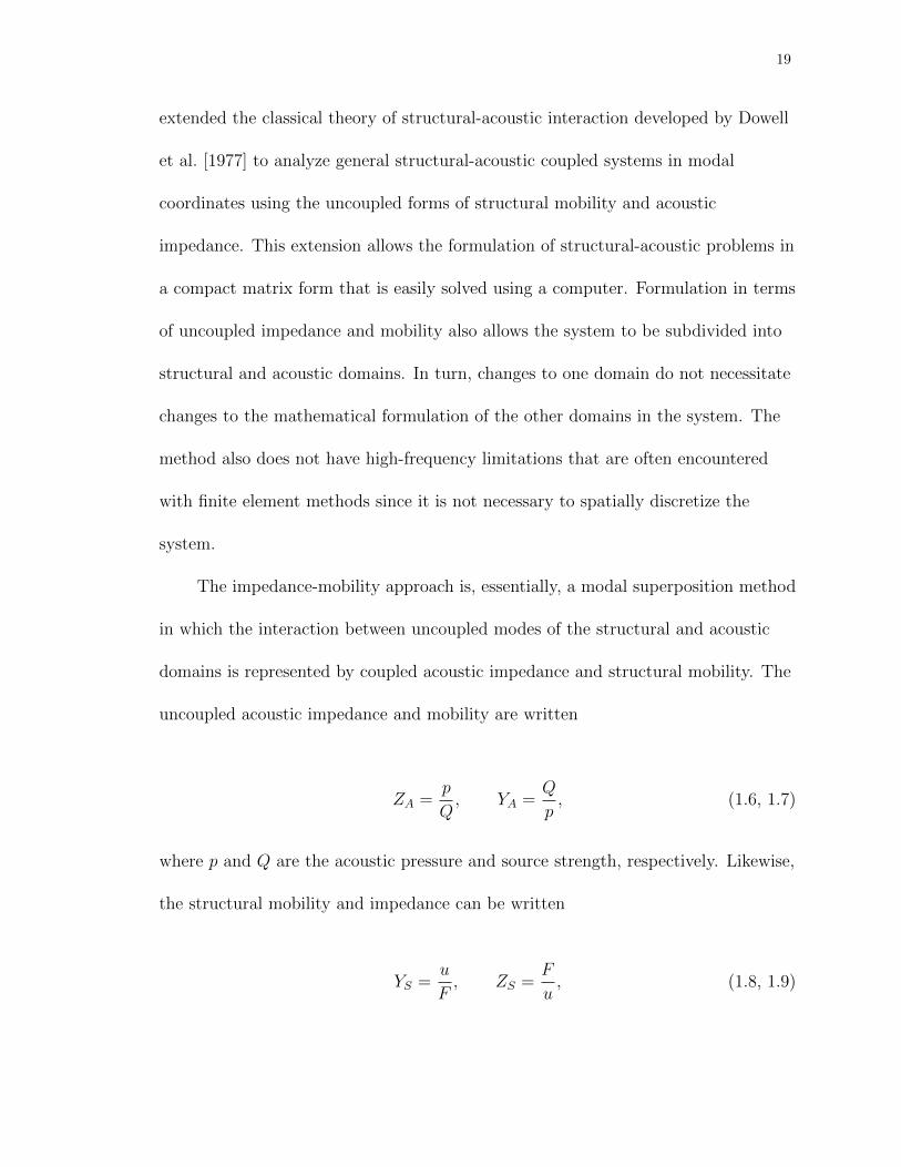
19

extended the classical theory of structural-acoustic interaction developed by Dowell

et al. [1977] to analyze general structural-acoustic coupled systems in modal

coordinates using the uncoupled forms of structural mobility and acoustic

impedance. This extension allows the formulation of structural-acoustic problems in

a compact matrix form that is easily solved using a computer. Formulation in terms

of uncoupled impedance and mobility also allows the system to be subdivided into

structural and acoustic domains. In turn, changes to one domain do not necessitate

changes to the mathematical formulation of the other domains in the system. The

method also does not have high-frequency limitations that are often encountered

with finite element methods since it is not necessary to spatially discretize the

system.

The impedance-mobility approach is, essentially, a modal superposition method

in which the interaction between uncoupled modes of the structural and acoustic

domains is represented by coupled acoustic impedance and structural mobility. The

uncoupled acoustic impedance and mobility are written

ZA =p

Q, YA =

Q

p, (1.6, 1.7)

where p and Q are the acoustic pressure and source strength, respectively. Likewise,

the structural mobility and impedance can be written

YS =u

F, ZS =

F

u, (1.8, 1.9)

20

where u and F are the resulting velocity and applied force, respectively. An analysis

of the dimensions of Equations (1.6)-(1.9) reveals a mismatch, with the units of ZS

being [Ns/m] and those of ZA being [Ns/m5]. This suggests a need for a coupling

factor to analyze structural-acoustic coupled systems. Kim & Brennan [1999]

introduced the terms of coupled acoustic impedance and coupled structural mobility,

ZCA =FAu, YCS = −QS

p, (1.10, 1.11)

where the new terms FA and QS are the acoustic reaction force, and the structural

source strength, respectively.

In the general modal superposition scheme, the field variables (displacement,

pressure, velocity, etc.) are written as the summation of the products of mode shape

functions and modal amplitudes. For the cases of pressure and velocity, the

equations are

p(x, ω) =N∑

n=1

ψn(x)an(ω) = ΨTa, (1.12)

and

u(y, ω) =M∑

m=1

φm(y)bm(ω) = ΨTb, (1.13)

respectively, where x and y are the acoustic and structural coordinates, ω is

frequency, ψn and φm are acoustic and structural mode shape functions, and an and

bm are the modal amplitudes. In matrix form Ψ and a are the N length arrays of

uncoupled acoustic modeshapes and modal acoustic pressure amplitudes. Φ and b

are the M length arrays of uncoupled structural mode shapes and modal structural

21

vibration amplitudes.

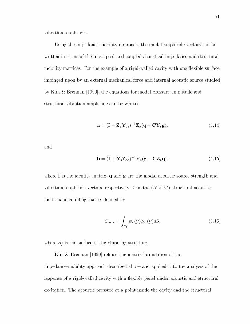
Using the impedance-mobility approach, the modal amplitude vectors can be

written in terms of the uncoupled and coupled acoustical impedance and structural

mobility matrices. For the example of a rigid-walled cavity with one flexible surface

impinged upon by an external mechanical force and internal acoustic source studied

by Kim & Brennan [1999], the equations for modal pressure amplitude and

structural vibration amplitude can be written

a = (I + ZaYcs)−1Za(q + CYsg), (1.14)

and

b = (I + YsZca)−1Ys(g −CZaq), (1.15)

where I is the identity matrix, q and g are the modal acoustic source strength and

vibration amplitude vectors, respectively. C is the (N ×M) structural-acoustic

modeshape coupling matrix defined by

Cm,n =

∫

Sf

ψn(y)φm(y)dS, (1.16)

where Sf is the surface of the vibrating structure.

Kim & Brennan [1999] refined the matrix formulation of the

impedance-mobility approach described above and applied it to the analysis of the

response of a rigid-walled cavity with a flexible panel under acoustic and structural

excitation. The acoustic pressure at a point inside the cavity and the structural

22

vibration velocity on the flexible panel were predicted, and showed good agreement

with experimental results. Lau & Tang [2001] used the impedance-mobility

approach to study the active control of a sound field in a rectangular enclosure.

They highlighted the flexibility of the impedance-mobility approach to analyze

structural-acoustic coupled systems.

Ouisse et al. [2005] developed a method based on impedance and mobility

concepts called the patch transfer function (PTF) approach which discretizes the

coupling surface between sub-domains into elementary surfaces, rather than nodes

which are commonly used in finite element methods. This method has been used to

study transmission loss of double panels [Chazot & Guyader 2007], the structural

and acoustic velocities of micro-perforated panels [Maxit et al. 2012], positioning of

absorbing material [Totaro & Guyader 2012], and more.

The research in this dissertation implements the impedance-mobility approach

to study membrane-type acoustic metamaterials due to its inherent computational

efficiency and flexibility. Optimization requires many iterations to converge on a

solution, and inefficient modeling methods become prohibitively time-consuming.

The flexibility of the impedance-mobility approach also allows the analysis to be

extended to include other structural or acoustic systems.

1.3.3 Genetic Algorithms

Optimization is the process of iteratively improving upon a solution to a given

problem by using information gained from previous trials until the most suitable

23

solution is found, subject to pre-defined criteria. There are many types of algorithms

for optimization, each with its own inherent advantages and disadvantages.

Evolutionary algorithms (EAs) have become popular in recent decades due to their

ability to converge on globally optimal solutions as opposed to converging on locally

optimal solutions or failing to converge entirely, which are common problems with

mathematical optimization. EAs are also convenient when dealing with problems

with many variables and non-linear objective functions [Elbeltagi et al. 2005]. In

addition EAs usually do not require derivatives, unlike gradient-based methods, and

therefore can be applied to non-differentiable functions.

Several types of EAs exist today that draw influence from the natural world.

Genetic algorithms (GAs) are based on the process of Darwinian evolution through

natural selection, crossover, and mutation [Holland 1975]. Memetic algorithms

(MAs) are similar to GAs and incorporate the ability for individuals, or “memes”, to

gain experience or learn [Merz & Freisleben 1997]. Particle swarm optimization

(PSO) is inspired by the social behavior of migrating birds in which each bird tries

to find the best position in the flock [Kennedy 1997]. Ant colony optimization

(ACO) draws from the social behavior of ants finding the shortest distance between

a food source and their nest by tracking pheromone trails [Dorigo et al. 1996].

Due to their inherent ability to handle large numbers of input parameters of

various types, GAs are chosen to optimize unit cells of membrane-type acoustic

metamaterials. GAs are also well-known for converging on globally optimal

solutions, so they are well-suited to design applications.

Genetic algorithms are numerical optimization methods inspired by the

24

processes of biological evolution and natural selection, in which the most fit

individuals survive to pass on their genetic information to the next generation

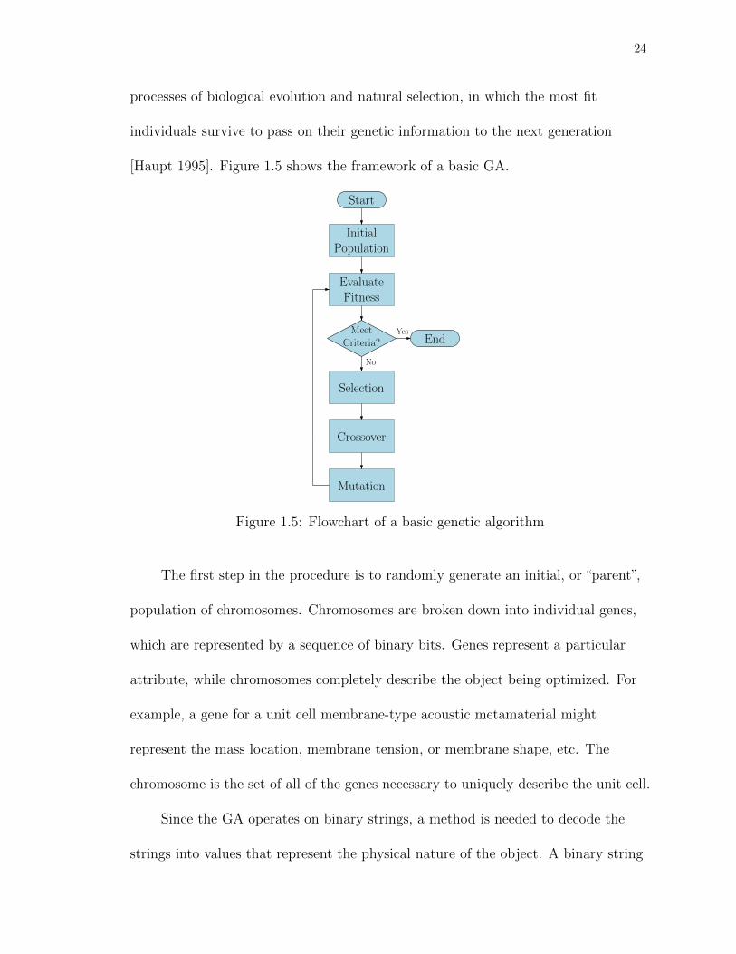
[Haupt 1995]. Figure 1.5 shows the framework of a basic GA.

InitialPopulation

EvaluateFitness

Crossover

Mutation

MeetCriteria?

No

Yes

Selection

End

Start

Figure 1.5: Flowchart of a basic genetic algorithm

The first step in the procedure is to randomly generate an initial, or “parent”,

population of chromosomes. Chromosomes are broken down into individual genes,

which are represented by a sequence of binary bits. Genes represent a particular

attribute, while chromosomes completely describe the object being optimized. For

example, a gene for a unit cell membrane-type acoustic metamaterial might

represent the mass location, membrane tension, or membrane shape, etc. The

chromosome is the set of all of the genes necessary to uniquely describe the unit cell.

Since the GA operates on binary strings, a method is needed to decode the

strings into values that represent the physical nature of the object. A binary string

25

of B bits can be converted to an integer via

Int =B∑

i=1

Bin(B − i+ 1) · 2i−1, (1.17)

where Bin is the binary string and its argument is the bit location ranging from 1

to B. Once an integer value, Int, is obtained, the result can be scaled to fit the

range of values that the parameter, x, can take by specifying a minimum and

maximum value, xmin and xmax respectively, and applying the equation

x = xmin +xmax − xmin

2B − 1Int. (1.18)

The next step of the GA is to evaluate the fitness, sometimes termed “cost”, of

each parent. To do this a fitness or cost function that represents the goals of the

optimization procedure is necessary. For example, a fitness function that optimizes

broadband transmission loss might be written

Fi =

∫ ωmax

ωmin

TL(ω)dω (1.19)

where Fi is the fitness score from the ith parent where i = 1 . . . N , and ωmin and

ωmax are the lower and upper bounds of the frequency range of interest. Another

fitness function that optimizes TL at 500 Hz, for example, might be written

Fi = TL(500Hz). (1.20)

26

It is important to note that as the fitness increases, so does the value of the fitness

function.

Each parent is then sorted according to its fitness score. At this point if the

population meets a specified stopping criterion, the GA is finished and the most fit

parent is the optimal solution. Typically, though, the process is not stopped until

convergence is reached, where the fitness scores for each parent in the population are

very close or identical.

If the stopping criterion is not met, the parents undergo the process of

selection, wherein the most fit survive to pass on their genetic information. This step

allows for some creativity on the part of the programmer in deciding which parents

survive. A typical scheme is to keep the most fit half of the parent population. In

this scheme each set of parents creates two new offspring, therefore the total

population size remains constant. It is helpful in this scheme if the population size

is divisible by four. Another scheme, known as proportional crossover, uses the

fitness score to assign a probability of survival Si to each parent, such as

Si =Fi∑Nj=1 Fj

(1.21)

Goldberg & Deb 1991. This, of course, necessitates that the fitness scores be

positive values. This scheme introduces some randomness, where even less fit

parents have some chance of producing offspring.

The next step in the GA is to create the next generation through the process of

crossover. Two parents are chosen according to some scheme. One common

27

selection method is to choose the most and least fit surviving parents, then the

second- most and second-least fit, etc. This ensures some degree of genetic diversity.

Another method is to choose the most and second-most fit, the third and fourth

most fit, etc. This is yet another parameter that gives the programmer some degree

of control over the convergence of the algorithm. After selection of the parents,

crossover occurs to create the next generation. The most commonly employed

crossover scheme is single-point crossover, where a point in the chromosome is

chosen to break and swap the bits to the right [Mitchell 1998]. This results in a new

chromosome with some number of bits from each parent. In Figure 1.6 a crossover

point of three is used to create the new chromosome. Notice that the first three bits

of the first parent, in red, and the remaining seven from the second, in blue, are

chosen to create the new chromosome. Multi-point crossover is another technique

where multiple crossover points are chosen and the bits between two points are

swapped between parents [De Jong & Spears 1992]. Multi-point crossover is most

effective when the number of bits per chromosome is high.

101001010110110101111001010111

CrossoverPoint

1011000111

Mutation

Figure 1.6: Example of single point crossover and mutation

Mutation introduces some degree of randomness to the GA to help ensure

genetic diversity and convergence on a globally optimal solution. In mutation a

random bit in a chromosome is altered, from zero to one or vice versa, according to

some rate defined by the programmer. A higher mutation rate generally means more

28

genetic diversity in later stages of the algorithm, leading to a more thorough

sampling of the search space. The process of mutation is shown in Figure 1.6 where

the sixth bit of the chromosome is changed from a one to a zero, shown in green.

GAs have many lucrative benefits over non-evolutionary optimization

techniques, such as direct search and gradient-based methods. Direct search relies

solely upon the objective function and its constraints, requiring many function

evaluations resulting in slow convergence. Gradient-based methods are not efficient

when applied to non-differentiable or discontinuous problems. Both methods tend to

be inefficient when handling discrete variables, and converge on local rather than

global optimums [Deb 1999]. These limitations are overcome by GAs.

GAs are well matched to optimize unit cells of metamaterials due to their unit

cell substructure, and have recently gained the attention of metamaterials

researchers. Li et al. [2012] applied GAs to design unit cells for gradient refractive

index (GRIN) lenses by optimizing the refractive index and impedance mismatch.

Since a relatively inefficient finite element method was used, the genetic algorithm

took approximately one week to converge upon an optimal solution. Silva et al.

[2014] used GAs to control the radiation patterns of phased-array radar systems.

They implemented maximum-minimum crossover, meaning that the most fit and

least fit solutions were mated through crossover to produce the next generation.

This ensures high genetic diversity and promotes convergence on a globally optimal

solution. Jiang et al. [2011] implemented a GA to design infrared

zero-index-metamaterials consisting of a dielectric layer sandwiched between two

metallic screens by optimizing impedance and refractive index. Meng et al. [2012]

29

optimized the underwater sound absorption of locally resonant acoustic

metamaterials based on the sonic crystal structure.

This dissertation addresses the problem of designing optimal unit cell

configurations of membrane-type acoustic metamaterials to attenuate airborne

sound. The response of a unit cell is modeled using a computationally efficient

impedance-mobility approach, and optimized using a genetic algorithm.

1.4 Dissertation Structure

To address the limitations caused by computationally inefficient models on design

and optimization applications, impedance-mobility modeling of membrane-type

acoustic metamaterials is described in Chapter 2. The model is first formulated for

a single unit cell, and then extended to multiple layers, arrays, and layers of arrays.

The modeshape of a membrane carrying a concentrated mass is rigorously

investigated to determine any potential limitations.

Chapter 3 verifies the accuracy of the impedance-mobility models using a finite

element method. The assumptions in the model are also investigated and validated

using the same method. The generalization of rectangular unit cell shapes to unit

cells of other geometries is explored.

The application of genetic algorithms to optimize the transmission loss

characteristics of membrane-type metamaterial structures is discussed in Chapter 4.

The formulation of fitness functions to meet specific design criteria is discussed in

detail.

30

Chapter 5 presents the results of the impedance-mobility models with

parameters optimized using genetic algorithms. Case studies of specific noise control

criteria and structures optimized to meet those criteria are presented.

Chapter 6 discusses the work done, its contributions to the field, and concludes

with recommendations for future work.

31

Chapter 2

Impedance-Mobility Modeling

This chapter describes the formulation of efficient dynamic models for

membrane-type acoustic metamaterials using the impedance-mobility approach.

Models for a single unit cell, unit cells arrayed in parallel, and unit cells stacked in

series are presented here. Quantities derived from the impedance-mobility approach

that are useful for design and optimization are also discussed.

A single unit cell of a membrane-type acoustic metamaterial consists of a

tensioned membrane carrying an attached mass supported by a rigid grid as seen in

Figure 2.1. To model the transmission loss (TL) of a unit cell of a membrane-type

acoustic metamaterial, the dynamic response of a membrane carrying an attached

mass must be analyzed with consideration given to coupling of the surrounding

fluid. The model can then be extended to examine the response of many unit cells

arrayed in parallel, stacked in series, or both. This chapter begins with the

formulation of a dynamic model for a single unit cell in a waveguide and expands

the analysis to larger systems.

32

Lx

Ly

(x0, y0)

lx

ly

Figure 2.1: Schematic of rectangular unit cell

2.1 Unit Cell

The equation of motion for a membrane carrying an attached mass can be written

as

ρs∂2w

∂t2+ ρmassh(x, y, x0, y0, lx, ly)

∂2w

∂t2− T∇2w = 2pince

jωt − 2ρ0c0∂w

∂t, (2.1)

where w is the transverse deflection of the membrane, ρs and T are the surface

density and applied tension of the membrane, respectively, and ρmass is the surface

density of the attached mass [Kopmaz & Telli 2002]. The amplitude of the incident

plane wave is pinc. The characteristic impedance of the fluid medium is given by

ρ0c0, and angular frequency is given by ω. A combination of four Heaviside unit-step

33

functions, denoted H , is used to characterize the finite attached mass as follows

h(x, y, x0, y0, lx, ly) = [H (x− x0)−H (x− x0 − lx)]

· [H (y − y0)−H (y − y0 − ly)] .(2.2)

This function takes a value of 1 on the surface of the attached mass and 0 elsewhere

on the membrane.

The formulation in Equation (2.1) assumes that the attached mass does not

impede bending in the membrane, and that its rotational inertia is negligible. These

assumptions are validated using finite element models in Chapter 3. A further

assumption is that the membrane is limp and that its stiffness does not contribute

significantly to the restoring force relative to the applied tension. The effect of

membrane stiffness is explored in Section 2.1.2.

The transverse deflection of the membrane can be written using mode

superposition as

w(x, y, t) =M∑

m=1

φm(x, y)qm(t), (2.3)

where φm(x, y) is the mode function which satisfies the boundary conditions, and

qm(t) is the time-dependent modal amplitude qm(t) = qmejωt. Substituting

Equation (2.3) into Equation (2.1), multiplying by an orthogonal mode function

φn(x, y) and integrating over the surface of the membrane, the following equation is

obtained

−ω2Mmqm − ω2

N∑

n=1

Qm,nqn +Kmqm = 2pincHm − jωDmqm. (2.4)

34

Equation (2.4) can be written in matrix-vector form as

−ω2 {[M ] + [Q]} q + jω {D} q + [K] q = 2pincH . (2.5)

The elements of the diagonal modal mass matrix, M , are given by

Mm = ρs

∫ Lx

0

∫ Ly

0

φm

N∑

n=1

φndydx. (2.6)

The elements of the matrix Q corresponding to the attached mass are given by

Qm,n = ρmass

∫ x0+lx

x0

∫ y0+ly

y0

φmφndydx. (2.7)

The damping due to air loading is given by D with elements

Dm = 2ρ0c0

∫ Lx

0

∫ Ly

0

φm

N∑

n=1

φndydx (2.8)

The stiffness matrix K is the diagonal matrix of elements given by

Km = −T∫ Lx

0

∫ Ly

0

φm∇2

N∑

n=1

φndydx. (2.9)

The modal volume displacement vector, H , is given by

Hm =

∫ Lx

0

∫ Ly

0

φmdydx. (2.10)

35

The modal mobility matrix can be derived from Equation (2.5) as

Y =jω

−ω2 {[M ] + [Q]}+ jω[D] + [K], (2.11)

and the modal vibration velocity amplitude is given by

V = Y gp, (2.12)

where gp is the generalized modal force vector due to the incident plane wave given

by

gp,m = 2

∫ Lx

0

∫ Ly

0

pincφmdydx. (2.13)

For frequencies in the plane wave regime of the waveguide, the sound pressure

transmission coefficient can be written

tp =

∣∣∣∣ρ0c0 〈v〉pinc

∣∣∣∣ , (2.14)

where 〈v〉 is the average velocity of the vibrating structure on the receiving side, and

pinc is the incident pressure amplitude [Chen et al. 2014a; Zhang et al. 2012]. The

displacement of a vibrating structure can be written in terms of normal modes as

v(x, y) =M∑

m=1

φm(x, y)Vm = ΦTV , (2.15)

where Φ is the column vector of area-normalized structural modeshapes, φm. The

36

average velocity can then be written

〈v〉 =1

LxLy

∫ Lx

0

∫ Ly

0

v(x, y)dydx =1

LxLyHTV . (2.16)

The transmission coefficient is then written

tp =

∣∣∣∣ρ0c0H

TV

LxLypinc

∣∣∣∣ , (2.17)

where superscript T denotes vector transpose. The transmission loss can then be

written

TL = −20 log10(tp). (2.18)

2.1.1 Baffled Transmission Loss

The transmitted sound power of a single unit cell in an infinitely extended rigid

baffle can be calculated using the power transfer matrix based on modal radiation

efficiencies [Fahy & Gardonio 2007; Snyder & Tanaka 1995]. The power transfer

matrix, [A], for modes α = (pα, qα) and β = (pβ, qβ) is given by

Aαβ =ρ0c0LxLy

64

(1 + (−1)pα+pβ

) (1 + (−1)qα+qβ

){pαqαpβqβ

σα +pβqβpαqα

σβ

}, (2.19)

where σα and σβ are the radiation efficiencies of modes α and β, respectively, given

by Wallace [1972] and in Appendix A. The total radiated sound power is given by

Πrad = V H [A]V . (2.20)

37

The sound power of the normally-incident plane wave is given by

Πinc =|pinc|2LxLy

2ρ0c0

. (2.21)

The transmission loss is then

TL = −10 log10

(Πrad

Πinc

). (2.22)

2.1.2 Membrane Stiffness

In the study of vibrating panels it is often assumed that the panel behaves either as

a membrane or a plate [Kinsler et al. 2000]. The distinction is in the restoring force

in the equation of motion. A membrane’s restoring force is due to an applied

tension, whereas the restoring force of a plate is due to its flexural rigidity. This

assumption also holds for the modeling of membrane-type acoustic metamaterials.

In most analytical models, a membrane model is used [Langfeldt et al. 2015; Tian

et al. 2014; Zhang et al. 2012], while some use a plate model [Lu et al. 2016; Li et al.

2014]. Chen et al. published two papers on the subject, one with a membrane model

[Chen et al. 2014a], and one with a plate model [Chen et al. 2014b].

The fact is, however, that the vibratory motion of any real structure is

influenced by both its flexural rigidity and any applied tension [Leissa 1969]. In the

present research, both are considered. This section and A.1.3 discuss the addition of

bending stiffness to a membrane model. Since the degree to which the tension and

stiffness affect the TL of the unit cell varies with configuration, in some cases it may

38

be appropriate to neglect one or the other.

An underlying assumption in the equation of motion given by Equation (2.1) is

that the bending stiffness of the membrane is negligible compared to the applied

tension. There may exist, however, certain design scenarios in which stiffer materials

are more suitable. This section outlines the adaptation of the single unit cell

impedance-mobility model to include the effects of membrane bending stiffness.

Generally, the equation of motion for a membrane or thin plate with both

in-plane tension and bending stiffness can be written [Leissa 1969]:

D∇4w − T∇2w = −ρs∂2w

∂t2, (2.23)

where D is the flexural rigidity of the membrane given by

D =Eh3

12(1− ν2), (2.24)

which is dependent upon the Young’s Modulus, E, Poisson’s Ratio, ν, and

thickness, h, of the membrane.

Incorporating the additional stiffness term into Equation (2.1) and following

the same derivation as above, Equation (2.5) becomes:

−ω2 {[M ] + [Q]} q + jω {D} q + [K] q + [E] q = 2pincH , (2.25)

where E is the diagonal stiffness matrix due to the flexural rigidity of the membrane

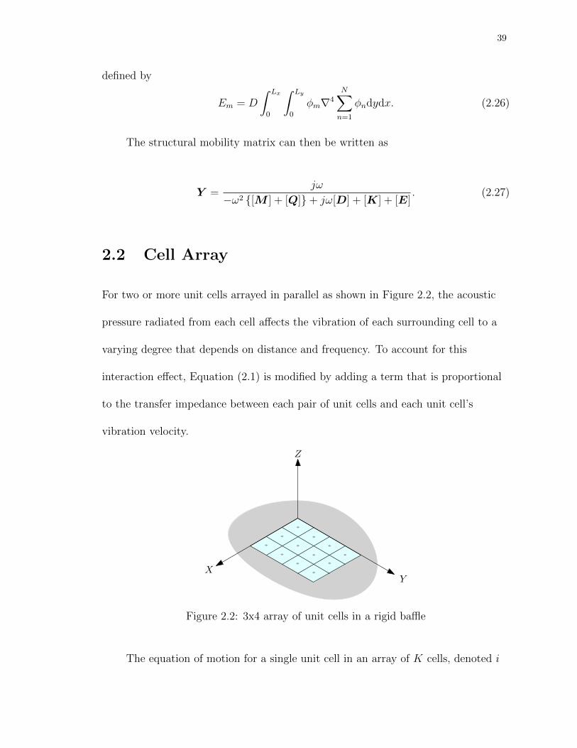
39

defined by

Em = D

∫ Lx

0

∫ Ly

0

φm∇4

N∑

n=1

φndydx. (2.26)

The structural mobility matrix can then be written as

Y =jω

−ω2 {[M ] + [Q]}+ jω[D] + [K] + [E]. (2.27)

2.2 Cell Array

For two or more unit cells arrayed in parallel as shown in Figure 2.2, the acoustic

pressure radiated from each cell affects the vibration of each surrounding cell to a

varying degree that depends on distance and frequency. To account for this

interaction effect, Equation (2.1) is modified by adding a term that is proportional

to the transfer impedance between each pair of unit cells and each unit cell’s

vibration velocity.

Z

YX

Figure 2.2: 3x4 array of unit cells in a rigid baffle

The equation of motion for a single unit cell in an array of K cells, denoted i

40

where i = 1, 2...K, with general external pressures, pext,i due to arbitrary sources is

written as

ρs∂2wi∂t2

+ ρmassh(x, y, x0, y0, lx, ly)∂2wi∂t2− T∇2wi = 2pince

jωt + 2pext,iejωt. (2.28)

pext,i can be written as a sum of contributions from each unit cell in the array

as

pext,i =K∑

j=1

pij. (2.29)

The pressure on any individual unit cell due to the vibration of adjacent unit

cells can be approximated by assuming that the array behaves as a set of elementary

piston-like radiators. This approximation is valid when the characteristic dimension,

a, of the unit cell is much less than the acoustic and flexural wavelength,

a =√LxLy � λ. From Rayleigh’s integral the pressure at one unit cell due to the

vibration velocity of another can be related through self- and mutual- radiation

impedances (see Appendix B of Chazot & Guyader 2007). The radiation impedance

is defined as the ratio of pressure at unit cell i due to the average vibration velocity

at unit cell j, given by

Zij =pi〈V 〉j

(2.30)

Zij =

ρ0c[1− e−jka] if i = j

jωρ0LxLy2π

e−jkdij

dijif i 6= j

(2.31)

where dij is the distance between centers of unit cells i and j. Equation (2.29) can

41

be rewritten as

pext,i =K∑

j=1

Zij〈V 〉j = jωK∑

j=1

Zij〈w〉j, (2.32)

where 〈w〉j is the spatially averaged displacement of cell j calculated by

〈w〉j =1

LxLy

∫ Lx

0

∫ Ly

0

wjdydx. (2.33)

The average displacement can be rewritten using the mode superposition in

Equation (2.3) and the definition of modal displacement given by Equation (2.10) as

〈w〉j =1

LxLy

M∑

m=1

Hmqm,jejωt =

1

LxLyHT qje

jωt. (2.34)

Substituting Equations (2.34), (2.32) and (2.3) into Equation (2.28) and, without

loss of generality, omitting the ejωt convention gives

− ω2ρs

M∑

m=1

φmqm,i − ω2ρmasshM∑

m=1

φmqm,i − T∇2

M∑

m=1

φmqm,i

= 2pinc +2jω

LxLy

K∑

j=1

ZijHT qj . (2.35)

Multiplying Equation (2.35) by φn, integrating over surface of cell i and using

orthogonality properties gives

− ω2Mm,iqm,i − ω2

N∑

n=1

Qm,n,iqn,i +Km,iqm,i

= 2pincHm +2jω

LxLyHm

K∑

j=1

ZijHT qj . (2.36)

42

In matrix-vector form, Equation (2.36) is

−ω2 {[Mi] + [Qi]} qi + [Ki] qi = 2pincH +2jω

LxLyHT [q] ZiH , (2.37)

where the bracketed [q] is the matrix formed by modal amplitude vectors for each of

K cells

[q] = bq1, q2, . . . , qKc, (2.38)

and {Zi} is the vector of transfer impedances

{Zi} = bZi,1, Zi,2, . . . , Zi,KcT . (2.39)

To solve for the modal amplitude vector qi, the components of [q] and {Zi}

corresponding to the ith cell are separated, leaving

[q′i] = bq1, . . . , qi−1, qi+1, . . . , qKc, (2.40)

and

{Z′i} = bZi,1, . . . , Zi,i−1, Zi,i+1, . . . , Zi,KcT . (2.41)

The elements of {Z′i} are given by Equation (2.31) for i 6= j.

43

Equation (2.37) then becomes

− ω2 {[Mi] + [Qi]} qi + [Ki] qi

= 2pincH +2jω

LxLyZi,iH

THqi +2jω

LxLyHT [q′i] {Z′i}H . (2.42)

Solving for qi gives

qi =2pincH + 2jω

LxLyHT [q′i] {Z′i}H

−ω2 {[Mi] + [Qi]}+ [Ki]− 2jωLxLy

Zi,iHTH. (2.43)

2.2.1 2 x 1 Array

Note that the vibration amplitude vector for each unit cell is a function of the

vibration amplitude vectors for all other unit cells in the array. This necessitates

solving a system of K equations and K unknown vectors, which can be difficult. In

this section the transmission loss of an array consisting of K = 2 unit cells is derived

to illustrate the process of expanding the analysis to multi-celled arrays.

The modal vibration amplitude vectors for unit cell 1 and 2 are written using

Equation (2.43)

q1 =2pincH + 2jω

LxLyZ12H

T q2H

−ω2 {[M1] + [Q1]}+ [K1]− 2jωLxLy

Z11HTH, (2.44)

and

q2 =2pincH + 2jω

LxLyZ21H

T q1H

−ω2 {[M2] + [Q2]}+ [K2]− 2jωLxLy

Z22HTH, (2.45)

44

respectively. Note that in the second term in the numerator of each equation

[q′1] = q2 and [q′2] = q1, respectively, and that {Z′1} and {Z′2} become scalar values

Z12 and Z21.

For convenience in notation, the matrix that corresponds to the equation of

motion of the ith unit cell can be defined as

[Σi] = −ω2 {[Mi] + [Qi]}+ [Ki]−2jω

LxLyZiiH

TH . (2.46)

Substituting Equation (2.45) into (2.44) and using (2.46), the fully coupled

modal vibration amplitude vectors are written

q1 =2pincH + 2jω

LxLy2pincZ12H

T [Σ2]−1 HH

[Σ1] + 4ω2

(LxLy)2Z12Z21HT [Σ2]−1 HHHT

, (2.47)

and

q2 =2pincH + 2jω

LxLy2pincZ21H

T [Σ1]−1 HH

[Σ2] + 4ω2

(LxLy)2Z21Z12HT [Σ1]−1 HHHT

. (2.48)

The total sound power radiated from the array is calculated by considering

each unit cell as a piston radiator in an infinite rigid baffle, with velocity equal to its

average value across the unit cell. The average velocity is calculated by

〈V 〉j = jω〈w〉j, (2.49)

where 〈w〉j is given by dropping the ejωt from Equation (2.34). The total radiated

45

sound power is then given by

Πrad = V He [R]Ve, (2.50)

where Ve is the vector of elementary velocities given by

Ve =

〈V 〉1

〈V 〉2

, (2.51)

and [R] is the radiation resistance matrix [Fahy & Gardonio 2007] defined for K = 2

elements by

[R] =ω2ρ0A

2e

4πc

1 sin kd12kd12

sin kd21kd21

1

, (2.52)

where dij is the distance between unit cells i and j. The transmission loss can then

be calculated using the incident sound power,

Πinc =|pinc|2S2ρ0c0

, (2.53)

where S is the total area of the array, Equations (2.50), and (2.22).

2.2.2 Negligible Coupling Model

As illustrated in the previous section, expanding the analysis to a large number of

unit cells in an array can be challenging. To obtain an estimate of the total TL of

46

an array consisting of an arbitrary number of elements, while sacrificing some

accuracy, the effect of mutual coupling can be neglected. The assumption of

negligible coupling between unit cells allows the vibration velocity of each unit cell

to be calculated independently and combined to find the total sound power radiated

by the array. The velocity of an elementary radiator, Ve,i, of the ith unit cell is the

average velocity over the surface given by

Ve,i =1

LxLyHTYigp. (2.54)

The elementary velocities can be combined, as in the previous section, for K unit

cells in an array by using the radiation resistance matrix

[R] =ω2ρ0A

2e

4πc

1 sin kR12

kR12· · · sin kR1K

kR1K

sin kR21

kR211 sin kR2K

kR2K

.... . .

...

sin kRK1

kRK1

sin kRK2

kRK2· · · 1

. (2.55)

The total radiated sound power is then calculated using Equation (2.50).

2.3 Two Layers

Consider the cross section of a rigid walled cavity of dimension (Lx ×Ly ×Lz) set in

a waveguide with two simply supported membrane-type acoustic metamaterial unit

cells located at z = 0 and z = Lz, shown in Figure 2.3. The vibratory response of

47

Pi

Pr

Pt

Lx

Lz

A B

MA MB

Figure 2.3: Cross-section of two stacked unit cells

each unit cell is affected not only by the incident pressure, but by the pressure in

the cavity as well. This creates a coupled system of governing equations that must

be solved simultaneously to obtain the steady-state response.

The responses of the panels and cavity can be written as a summation of

normal modes. The cavity pressure p and panel velocities vi, where i is either A or

B, are written as

p(x, y, z, t) =N∑

n=1

ψn(x, y, z)Pn(t), (2.56)

vi(x, y, t) =M∑

m=1

φm(x, y)Vi,m(t), (2.57)

where ψn and φm are the normalized acoustic and structural modes given by

ψn(x, y, z) =√e1e2e3 cos

(n1πx

Lx

)cos

(n2πy

Ly

)cos

(n3πz

Lz

), (2.58)

48

where ei = 1 for ni = 0 and ei = 2 if ni > 0, and

φm(x, y) = 2 sin

(m1πx

Lx

)sin

(m2πy

Ly

). (2.59)

The governing equations for the coupled acoustic cavity pressure P , panel A velocity

VA, and panel B velocity VB are given in modal terms by [Jin et al. 2009]

Pn + 2ξnωnPn + ω2nPn =

ρ0c20

jωV

M∑

m=1

CAm,nVAm −

ρ0c20

jωV

M∑

m=1

CBm,nVBm, (2.60)

VAm + 2ξAmωAmVAm + ω2AmVAm =

jω

MAm

(gpm −

N∑

n=1

CAm,nPn

), (2.61)

and

VBm + 2ξBmωBmVBm + ω2BmVBm =

jω

MBm

N∑

n=1

CBm,nPn, (2.62)

respectively. The modal coupling coefficient, Cim,n, of the mth structural mode of the

ith unit cell to the nth acoustic mode of the cavity is given by

Cim,n =

∫ Lx

0

∫ Ly

0

ψn(x, y, zi)φm(x, y)dydx, (2.63)

where zi is the z-coordinate of the ith unit cell, either 0 or Lz.

49

Equations (2.60)-(2.62) can be written in matrix form as

P = Za(CAVA −CBVB), (2.64)

VA = YA(gp −CTAP ), (2.65)

and

VB = YBCTBP , (2.66)

respectively.

Combining the system of three equations and three unknown variables given by

Equations (2.64)-(2.66) and isolating the dependent variables gives

P = (I + ZaCAYACTA + ZaCBYBC

TB)−1ZaCAYAgp, (2.67)

VA =[I + YAC

TA(I + ZaCBYBC

TB)−1ZaCA

]−1YAgp, (2.68)

and

VB =[I + YBC

TB(I + ZaCAYAC

TA)−1ZaCB

]−1YB

·[CT

B(I + ZaCAYACTA)−1ZaCAYAgp

].

(2.69)

The uncoupled acoustic impedance [Kim & Brennan 1999; Dowell et al. 1977] of the

cavity Za is given by

Za =Aρ0c

20

V, (2.70)

50

where A is a diagonal matrix with elements given by

A1 =1

1/Ta + jω, (2.71)

for n = 1 and

An =jω

ω2n − ω2 + j2ζnωnω

, (2.72)

for n 6= 1.

The uncoupled structural mobility for panels A and B, YA and YB respectively,

can be written [Zhang et al. 2012; Fahy & Gardonio 2007]

Yi =jω

−ω2{[Mi] + [Qi]}+ jω[Di] + [Ki], (2.73)

where i denotes either panel A or B.

The sound pressure transmission coefficient can be written

tp =

∣∣∣∣ρ0c0 〈v〉pi

∣∣∣∣ , (2.74)

where 〈v〉 is the average velocity of the vibrating structure on the receiving side, and

pi is the incident pressure amplitude. The velocity of a vibrating structure can be

written in terms of normal modes as

v(x, y) =M∑

m=1

φm(x, y)VB,m = ΦTVB, (2.75)

51

where Φ is the column vector of area-normalized structural modeshapes, φm. The

average velocity can then be written

〈v〉 =1

LxLy

∫ Lx

0

∫ Ly

0

v(x, y)dydx =1

LxLyHTVB. (2.76)

The transmission coefficient is then written

tp =

∣∣∣∣ρ0c0H

TVB

LxLypinc

∣∣∣∣ , (2.77)

2.4 Derived Quantities

The flexibility of the impedance-mobility approach allows the derivation of several

quantities, in addition to TL, that may be useful to noise control engineers. When

discussing metamaterials, the idea of a negative effective dynamic mass often arises.

The reflection and absorption coefficients are important when considering the sound

field on both sides of the barrier. In active control, panel kinetic energy and cavity

potential energy are often used as control variables. The impedance-mobility

approach directly calculates modal displacement, velocity, and cavity pressure

amplitudes. This section delineates the equations necessary to derive useful

quantities from values calculated via the impedance-mobility approach.

52

2.4.1 Effective Dynamic Mass

The effective dynamic mass can be derived from Newton’s second law of motion

F = ma [Naify et al. 2010]. Likewise, the effective dynamic density can be found by

dividing by the surface area of the membrane [Yang et al. 2008]. The average force

due to acoustic excitation acting on the metamaterial unit cell is found using the

generalized modal force vector gp and the modal volume displacement vector H ,

〈F 〉 =HT gp

LxLy. (2.78)

The average out-of-plane acceleration is found using the modal velocity amplitude

vector, V , of the radiating unit cell and is given by

〈az〉 =jωV HH

LxLy, (2.79)

where superscript H denotes Hermitian transpose. Dividing Equation (2.78) by

Equation (2.79) gives the effective dynamic mass

meff =HT gp

jωV HH. (2.80)

2.4.2 Reflection and Absorption Coefficients

The sound pressure reflection coefficient is the ratio of reflected to incident sound

pressure. It is defined as

rp = 1− tp, (2.81)

53

where tp is the sound pressure transmission coefficient defined by Equation (2.17)

for a single unit cell in a waveguide, or Equation (2.77) for a double layer of unit

cells in a waveguide. The sound power transmission and reflection coefficients are

given by TΠ = |tp|2, and RΠ = |rp|2, respectively.

The sound absorption coefficient, α, is the fractional portion of the incident

energy that is not reflected or transmitted. It is calculated from the sound power

transmission and reflection coefficients as

α = 1− TΠ −RΠ. (2.82)

2.4.3 Panel Kinetic Energy

The kinetic energy of a vibrating panel is a useful quantity in active vibration

control. Membrane-type acoustic metamaterials are a prime candidate for active

structural control, since the vibration patterns directly influence the amount of

sound reflection. It is easy to imagine attaching a mechanical actuator to the

attached mass or replacing it with a piezoelectric actuator to actively control the

resonance frequencies. The kinetic energy of a vibrating surface can be written

Ek = ρs

∫ Lx

0

∫ Ly

0

|v(x, y, ω)|2 dydx. (2.83)

Jin et al. [2009] derived the kinetic energy of a panel using the impedance-mobility

approach as

Ek = ρsLxLyVHV . (2.84)

54

2.4.4 Cavity Potential Energy

For a membrane-type acoustic metamaterial configuration consisting of two unit

cells in series with an acoustic cavity between them, it may be useful to consider the

potential energy within the cavity. Once again, the ease of extending a double layer

configuration to actively control sound transmission loss is evident. By placing an

acoustic control source inside the cavity, the excitation of the radiating unit cell can

be minimized, reducing the amount of sound transmitted through the barrier. The

impedance-mobility approach greatly simplifies this extension.

The acoustic potential energy inside a rectangular cavity is defined as

Ep =1

4ρ0c20

∫ Lx

0

∫ Ly

0

∫ Lz

0

|p(x, y, z, ω)|2 dzdydx. (2.85)

Jin et al. [2009] derived the cavity potential energy using the impedance-mobility

approach in terms of the cavity modal pressure amplitude, P , as

Ep =V

4ρ0c20

PHP . (2.86)

2.5 Concluding Remarks

This chapter presents the formulation of impedance-mobility models of

membrane-type acoustic metamaterials in various configurations. The models of

single unit cells in a waveguide and in a baffle are extended to larger systems

comprised of multiple unit cells, either stacked in series in a waveguide, or arrayed

55

in parallel in a baffle. A fully-coupled formulation for a 2×1 array in a baffle is

presented, as well as a model with a negligible coupling assumption for an arbitrary

number of unit cells. Useful quantities are derived from the impedance-mobility

models, including effective dynamic mass, reflection and absorption coefficients,

panel kinetic energy, and cavity potential energy.

Implementing the impedance-mobility models presented in this chapter and

expanded upon in Appendices A and E results in computationally efficient dynamic

models of membrane-type acoustic metamaterials. These models are useful for

creating design tools, and optimization using iterative schemes. The verification of

these models is presented in Chapter 3.

56

Chapter 3

Finite Element Verification

This chapter presents the verification of the accuracy and the validation of

assumptions of the impedance-mobility models formulated in Chapter 2 using a

finite element method (FEM) [Zienkiewicz et al. 1977]. The assumptions that the

bending stiffness and rotary inertia of the attached mass are negligible are tested.

The generalization of the impedance-mobility model for rectangular membranes and

masses to systems of other shapes is also explored using FEM and presented in this

chapter. Circular, hexagonal, and triangular unit cell configurations are compared

to results of the impedance-mobility model which assumes a square unit cell of equal

area.

The acoustics module of the commercial FEM software package COMSOL

Multiphysics version 4.3 is used in this research. Unless otherwise noted, tetrahedral

elements are used with a quadratic shape function and a non-linear solver

[COMSOL Multiphysics 2012]. The impedance-mobility models are implemented

using custom scripts in MathWorks MATLAB 2015a. All FEM computations were

57

performed on a Windows server with two Intel Xeon E5-2670 2.6 GHz processors

and 16 gigabytes of RAM.

3.1 Verification of Accuracy

This section verifies the accuracy of the impedance-mobility approach by comparing

transmission loss results to those obtained using FEM models. FEM has been used

in previous studies of membrane-type acoustic metamaterials (see, for example,

Chen et al. 2014a; Naify et al. 2012; Yang et al. 2008) and compared against

experimental results, with good agreement. Naify et al. 2012 reported less than 10

percent difference between FEM and measured transmission loss (TL).

The TL curves of a single unit cell in a waveguide and a baffle, multi-cellular

arrays in baffles, and a double layer of unit cells in waveguide are verified using

FEM.

3.1.1 Unit Cell in a Waveguide

The FEM model used to verify the accuracy of the impedance-mobility model of a

single unit cell set in a rectangular waveguide is a three-dimensional

acoustic-structure interaction model. This model is the most realistic configuration,

using a finite thickness membrane and mass. Three boxes are used to represent the

membrane, mass, and waveguide geometry as shown in Figure 3.1 (A). In the

frequency range of interest from 100 Hz to 4000 Hz, only plane wave modes

propagate in the waveguide due to its small width and height compared to a

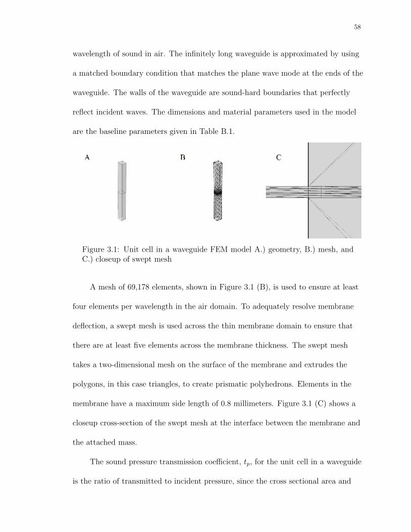
58

wavelength of sound in air. The infinitely long waveguide is approximated by using

a matched boundary condition that matches the plane wave mode at the ends of the

waveguide. The walls of the waveguide are sound-hard boundaries that perfectly

reflect incident waves. The dimensions and material parameters used in the model

are the baseline parameters given in Table B.1.

Figure 3.1: Unit cell in a waveguide FEM model A.) geometry, B.) mesh, andC.) closeup of swept mesh

A mesh of 69,178 elements, shown in Figure 3.1 (B), is used to ensure at least

four elements per wavelength in the air domain. To adequately resolve membrane

deflection, a swept mesh is used across the thin membrane domain to ensure that

there are at least five elements across the membrane thickness. The swept mesh

takes a two-dimensional mesh on the surface of the membrane and extrudes the

polygons, in this case triangles, to create prismatic polyhedrons. Elements in the

membrane have a maximum side length of 0.8 millimeters. Figure 3.1 (C) shows a

closeup cross-section of the swept mesh at the interface between the membrane and

the attached mass.

The sound pressure transmission coefficient, tp, for the unit cell in a waveguide

is the ratio of transmitted to incident pressure, since the cross sectional area and

59

fluid impedance are the same on both sides. The transmitted and incident pressures

are found by integrating over the end and beginning of the waveguide, respectively.

The TL is given by −20 log10 (tp).

Figure 3.2 shows the results of the impedance-mobility model (solid) and FEM

(dashed). In general, there is good agreement between the two methods. The TL

peak at 360 Hz and two resonance frequencies at 230 Hz and 3760 Hz, respectively,

are accurately captured with the impedance-mobility model within 2%. The

magnitude of the TL is also in good agreement with the FEM model, with a notable

exception near the TL peak and resonance frequencies where a lack of damping in

the FEM model is evident. This result is consistent with the difference between

FEM and TL measured in a plane wave tube by Naify et al. [2011b]. The

impedance-mobility model of a unit cell in waveguide accurately predicts TL for the

baseline configuration.

Frequency [Hz]100 500 1000 2000 3000 4000

Tra

nsm

issi

on L

oss

[dB

]

0

10

20

30

40

50

60

70

80

90

100Unit Cell in Waveguide FEM Verification

Impedance-MobilityFinite Element

Figure 3.2: FEM verification of a single unit cell in a waveguide. Impedance-mobility (solid), FEM (dashed)

60

3.1.2 Unit Cell in a Baffle

A second FEM model is used to verify the accuracy of the impedance-mobility

model of a single unit cell set in a rigid baffle. Due to computational limitations, a

two-dimensional shell model is used for the rigid baffle, membrane, and mass. This

reduces the three-dimensional solid structures to two-dimensional surfaces, and

equivalent parameters are automatically computed. The appropriateness of using a

two-dimensional shell to represent a three-dimensional structure is analyzed for the

simple case of a single unit cell in a waveguide in Section 3.2.1.

A rectangular waveguide is used on the incident side of the unit cell to limit

the excitation to normally incident plane waves. This ensures that there are no

spurious reflections of the plane wave off of the baffle or the air domain boundary.

On the transmitted side, a hemispherical air domain is used with a spherical

radiation boundary condition. This approximates sound radiating from the unit cell

to infinity with no reflections. The model geometry is shown in Figure 3.3 (A).

A two-dimensional mesh is used on the surface of the unit cell and baffle and

converted to match the tetrahedral mesh in the air domain, which is shown in

Figure 3.3 (B). A total of 68,939 mesh elements is used to maintain at least four

elements per wavelength at 4000 Hz.

Figure 3.4 shows a comparison of the results of the TL modeled in FEM and

using the impedance-mobility approach. The results are in good agreement,

accurately capturing the first and second resonance frequencies at 226 Hz and 3552

Hz, respectively, within 3%. There is a small discrepancy in the magnitude of the

61

Figure 3.3: Baffled unit cell FEM model A.) geometry, and B.) mesh.

Frequency [Hz]100 500 1000 2000 4000

Tra

nsm

issi

on L

oss

[dB

]

0

10

20

30

40

50

60

70

80

90

100Unit Cell in a Baffle FEM Verification


Figure 3.4: FEM verification of a single unit cell in a baffle. Impedance-mobility(solid), FEM (dashed)

first resonance and TL peak that is explained by a lack of damping in the FEM

model.

62

3.1.3 2×1 Array in a Baffle

To extend the model introduced in the previous section to analyze a system

consisting of an array of unit cells in a baffle, a second unit cell is placed adjacent to

the first sharing a common boundary in the FEM model as shown in Figure 3.5 (A).

The meshes in the air domain and membranes are identical to those used for the

single unit cell in a baffle. A total of 100,331 elements is used.

Figure 3.5: FEM geometry of baffled multi-cell arrays A.) 2×1 B.) 2×2

Figure 3.6 compares the TL from the impedance-mobility model with mutual

coupling between the two unit cells against FEM results. The impedance-mobility

model accurately predicts the TL of the 2×1 array below the second resonance

frequency, with less than 2% relative error in the TL peak at 350 Hz. However,

there is a discrepancy of about 9% at the second resonance at 3520 Hz where the

wavelength of sound in air is on the order of the dimensions of the array.

Due to the complexity of formulating an impedance-mobility model that

63

Frequency [Hz]100 500 1000 2000 4000

Tra

nsm

issi

on L

oss

[dB

]

0

10

20

30

40

50

60

70

80

90

1002x1 Array in a Baffle FEM Verification


Figure 3.6: FEM verification of a 2×1 array in a baffle. Impedance-mobility(solid), FEM (dashed)

incorporates mutual coupling between an arbitrary number of unit cells, it is also

desirable to verify the accuracy of the negligible coupling model formulated in

Section 2.2.2. Figure 3.7 shows the results of the impedance-mobility model with

negligible coupling compared to FEM. There is very good agreement between the

models with less than 2% relative error for each of the first and second resonances

and TL peak frequency at 230 Hz, 350 Hz, and 3530 Hz, respectively. This indicates

that mutual coupling of vibratory motion between unit cells does not significantly

contribute to the radiated sound power.

3.1.4 2×2 Array in a Baffle

Similarly, the model can be expanded to study a 2×2 array of unit cells in a baffle

using the geometry shown in Figure 3.5 (B). Comparing the negligible coupling

impedance-mobility model to the FEM results in Figure 3.8 again shows excellent

64

Frequency [Hz]100 500 1000 2000 4000

Tra

nsm

issi

on L

oss

[dB

]

0

10

20

30

40

50

60

70

80

90



Figure 3.7: FEM verification of a 2×1 array in a baffle. Impedance-mobilitywith negligible coupling assumption (solid), FEM (dashed)

agreement below the second resonance frequency.

Frequency [Hz]100 500 1000 2000 4000

Tra

nsm

issi

on L

oss

[dB

]

0

10

20

30

40

50

60

70

80

90



Figure 3.8: FEM verification of a 2×2 array in a baffle using negligible couplingmodel. Impedance-mobility (solid), FEM (dashed)

The results indicate that the negligible coupling impedance-mobility model

maintains accuracy while increasing the number of unit cells in the array. There is

less than 2% difference in the TL peak and resonance frequencies at 350 Hz, 230 Hz,

65

and 3520 Hz, respectively. The vastly simpler derivation of the negligible coupling

impedance-mobility model allows expansion to multi-cellular arrays to be explored

further in Chapter 5.

3.1.5 Double Layer in a Waveguide

A configuration of two unit cells stacked in series in a waveguide is modeled by

introducing a second unit cell to the FEM model described in Section 3.1.1 as shown

in Figure 3.9 (A). The second unit cell is placed 8 millimeters above the first so that

each unit cell has enough space to freely vibrate. For computational efficiency an

acoustic-shell interaction model is used that approximates the membranes as

two-dimensional surfaces. The mesh consists of 60,892 elements and is shown in

Figure 3.9 (B).

Figure 3.9: Double layer in a waveguide FEM A.) geometry and B.) mesh.

The results in Figure 3.10 show very good agreement of the TL predicted with

66

Frequency [Hz]100 500 1000 2000 4000

Tra

nsm

issi

on L

oss

[dB

]

0

10

20

30

40

50

60

70

80

90

100Double Layer in Waveguide FEM Verification


Figure 3.10: FEM verification of a double unit cell in a waveguide. Impedance-mobility (solid), FEM (dashed)

FEM and the impedance-mobility approach. The absolute value of the difference in

TL away from the resonances and TL peak is generally less than 1 dB. The

uncertainty of the resonance and TL peak frequencies is less than 3% as shown on

the plot, but cannot be adequately explored due to the low sampling frequency of

the FEM model.

3.2 Validation of Assumptions

Three important assumptions that are made in the impedance-mobility models

derived in Chapter 2 are tested in this section. The first assumption is that the

attached mass does not prohibit bending of the membrane segment on which it lies.

The second assumption is that the rotary inertia of the attached mass does not

affect the vibration of the membrane. Effectively, the impedance-mobility model

assumes a uniformly thick membrane with discontinuous surface density. These

67

assumptions are tested using FEM models that manipulate the geometry of the unit

cells to match the constraints of the impedance-mobility models. The third

assumption is that in an array of multiple unit cells, the mutual pressure between

unit cells acts evenly across the surface of each unit cell, and the unit cell behaves as

a piston-like radiator. This is tested by examining the surface pressure on the array,

and the deflection of the unit cells. The degree to which each of the assumptions is

valid is investigated.

3.2.1 Attached Mass Bending Stiffness

It is obvious that a material used for the attached mass is likely to have a much

higher bending stiffness than that of the membrane since denser materials are also

likely to be stiffer. An assumption made in the impedance mobility model is that the

difference in stiffnesses will have a negligible impact on the unit cell vibration and

transmission loss. In fact, a discontinuity in bending stiffness would be a violation of

the fundamental assumption in Equation (2.3). This is evident in Equation (2.26)

where the flexural rigidity, D, which is a measure of bending stiffness, is multiplied

by the square of the divergence of the gradient of the membrane deflection.

The bending stiffness of the attached mass is proportional to the cube of the

mass thickness, as seen in Equation (2.24). It is evident that the flexural rigidity of

the mass depicted in Figure 3.11 (A), will be higher than that depicted in

Figure 3.11 (B) or (C) due its increased thickness. To investigate the effects of mass

bending stiffness, a FEM model with simplified geometry consisting of an attached

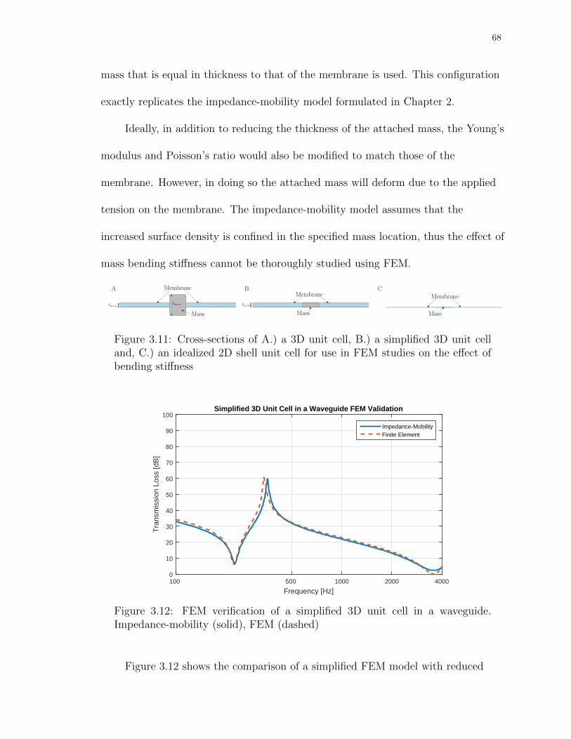
68

mass that is equal in thickness to that of the membrane is used. This configuration

exactly replicates the impedance-mobility model formulated in Chapter 2.

Ideally, in addition to reducing the thickness of the attached mass, the Young’s

modulus and Poisson’s ratio would also be modified to match those of the

membrane. However, in doing so the attached mass will deform due to the applied

tension on the membrane. The impedance-mobility model assumes that the

increased surface density is confined in the specified mass location, thus the effect of

mass bending stiffness cannot be thoroughly studied using FEM.

tmemtmass

Membrane

Mass

A

tmem

Membrane

Mass

BMembrane

Mass

C

Figure 3.11: Cross-sections of A.) a 3D unit cell, B.) a simplified 3D unit celland, C.) an idealized 2D shell unit cell for use in FEM studies on the effect ofbending stiffness

Frequency [Hz]100 500 1000 2000 4000

Tra

nsm

issi

on L

oss

[dB

]

0

10

20

30

40

50

60

70

80

90

100Simplified 3D Unit Cell in a Waveguide FEM Validation


Figure 3.12: FEM verification of a simplified 3D unit cell in a waveguide.Impedance-mobility (solid), FEM (dashed)

Figure 3.12 shows the comparison of a simplified FEM model with reduced

69

thickness of the attached mass, as shown in Figure 3.11 (B), to the

impedance-mobility model. There is good agreement between the two models with

less than 1% relative error at the resonances at 220 Hz and 3570 Hz and less than

5% error at the TL peak frequency 340 Hz. By comparing Figure 3.2 to Figure 3.12,

it is evident that as the assumptions in the FEM model are manipulated to match

those in the impedance-mobility model the level of agreement increases. By again

referring to Figure 3.2, it is clear that while the bending stiffness of the attached

mass (and its thickness) does affect the TL of the unit cell to a small degree, the

impedance-mobility model is still accurate despite the assumption that the effects

are completely negligible.

Additionally, the thickness of the unit cell can be neglected entirely in the

geometry of the FEM model (see Figure 3.11 (C)). By treating the unit cell as a

two-dimensional shell, the appropriateness of neglecting the thickness of the

membrane and attached mass in the impedance-mobility model can be further

validated.

For the shell model, a triangular mesh was used on the surface of the

membrane and attached mass and converted to match the tetrahedral elements in

the air domain. This resulted in 49,506 elements and 96,093 degrees of freedom.

Figure 3.13 shows the results of the shell FEM model compared to the

impedance-mobility approach. The TL results are nearly identical, with only minor

discrepancies of 3 dB in magnitude and 4% relative error at the second resonance at

3690 Hz and less than 5 dB in magnitude and less than 1% at the TL peak

frequency of 350 Hz.

70

Frequency [Hz]100 500 1000 2000 3000 4000

Tra

nsm

issi

on L

oss

[dB

]

0

10

20

30

40

50

60

70

80

90

100Unit Cell in a Waveguide Shell Model FEM Validation


Figure 3.13: FEM shell model verification of a single unit cell in a waveguide.Impedance-mobility (solid), FEM (dashed)

By comparing the TL from FEM models with varying attached mass

thicknesses, the assumption made in the impedance-mobility model that the

bending stiffness of the attached mass is negligible is tested. In general, the

impedance-mobility model accurately predicts TL for unit cells with non-negligible

attached mass stiffness.

3.2.2 Attached Mass Rotary Inertia

For attached masses that are relatively thin, the assumption that the rotary inertia

of the mass is negligible may be appropriate. However as mass size increases,

especially in the z direction, the impedance-mobility model may lose accuracy in

prediction. To study the influence of attached mass rotary inertia, a FEM model is

used where the thickness of the attached mass is varied, while maintaining the same

mass magnitude. Additionally, the location of the mass is varied to increase any

71

potential effects of attached mass rotation. Since the unit cell is excited by a

normally-incident plane wave, only symmetric modes are excited. This will result in

purely translational motion in the axial direction of a centrally-located attached

mass. An eccentric mass location produces the desired rotational motion that will

allow the effects of rotational inertia to be investigated, and the assumption in the

impedance-mobility model to be validated.

Frequency [Hz]100 500 1000 2000 4000

Tra

nsm

issi

on L

oss

[dB

]

0

10

20

30

40

50

60

70

80

90

100Transmission Loss of Unit Cell with Eccentric Mass Location


Figure 3.14: Comparison of impedance-mobility (solid) and FEM (dashed)transmission loss of a unit cell with an eccentric mass location

Figure 3.14 shows the results of the FEM model with an eccentrically placed

mass, the baseline configuration with x0 = 6 mm as defined in Figure 2.1, compared

to the impedance-mobility approach. At an eccentric location, the mass will

undergo non-uniform displacement across its area, resulting in out-of-plane mass

rotation. The effect of the rotary inertia of the attached mass is seen particularly at

460 Hz, where there is an additional TL peak. At this frequency, the mass

undergoes maximum rotation, as shown in Figure 3.15. The energy required to

72

rotate the attached mass is not radiated downstream of the unit cell, and thus a

peak in the TL curve appears.

Figure 3.15: Example of rotary inertia of the attached mass at 460 Hz fromFEM model

With the exception of the additional TL peak, the impedance-mobility model

performs well compared to FEM. The relative error is less than 6% at the resonance

at 3120 Hz, and less than 1% at the TL peak at 350 Hz. There is also some

discrepancy in the TL at the high end of the frequency range of less than 15 dB

near 4000 Hz.

Since the impedance-mobility model treats the attached mass as a

discontinuity in the surface density of the unit cell, the effects of attached mass

rotation are not adequately captured. This will lead to under-prediction of the TL

at the frequencies that excite rotation of the attached mass.

By decreasing the thickness of the attached mass, the effect of rotary inertia

can be studied further. A FEM model with eccentric mass location and thickness

equal to that of the membrane is used. The results shown in Figure 3.16 indicate

that the frequency at which the mass rotation produces a TL peak increases, while

decreasing the magnitude of the peak. The deflection of the unit cell at the TL peak

frequency is shown in Figure 3.17. The resonance occurs when the mass rotates on

73

its major axis in the plane and the membrane remains stationary.

Frequency [Hz]100 500 1000 2000 4000

Tra

nsm

issi

on L

oss

[dB

]

0

10

20

30

40

50

60

70

80

90

100Transmission Loss of Unit Cell with Eccentric Mass Location


Figure 3.16: Comparison of impedance-mobility (solid) and FEM (dashed)transmission loss of a unit cell with a reduced thickness eccentrically placedattached mass

Figure 3.17: Example of rotary inertia of the attached mass at 790 Hz

3.2.3 Coupling Between Unit cells in an Array

In Chapter 2 the formulation of an impedance-mobility model for an array of unit

cells in a baffle assumes that the pressure on one unit cell due to another is uniform

over its area. This assumption, however, does not hold for values of ka that are not

much less than unity (i.e. at high frequencies or large unit cell dimensions).

74

Figure 3.18 shows the pressure on the surface of two adjacent unit cells in a rigid

baffle at 3500 Hz. The pressure distribution on the unit cells is not uniform, with

higher pressure toward the center of the array. This causes asymmetric vibration of

the unit cells as shown in Figure 3.19.

Figure 3.18: Surface pressure of a 2×1 array of unit cells in a baffle

This result agrees with Naify et al. [2011b], who pointed out that pressure

coupling of adjacent unit cells causes an increase in the effective stiffness of the

membranes. As a result, the second resonance frequency increases. This suggests

that the impedance-mobility model of multi-cell arrays is only accurate below

approximately 2000 Hz.

3.3 Generalization to Other Unit Cell Geometries

The impedance-mobility formulation described in Chapter 2 is valid for unit cells

with rectangular geometry. It may arise, in some situations, that it is advantageous

to fabricate noise barriers of membrane-type acoustic metamaterials that do not

75

Figure 3.19: Displacement of a 2×1 array of unit cells in a baffle

have rectangular unit cells. For instance, drilling circular holes into a rigid matrix

may be more efficient than cutting squares. This section presents the comparison of

the transmission loss of membrane-type acoustic metamaterials with circular,

hexagonal, and triangular unit cell shapes using FEM. This comparison sheds light

on the degree to which the impedance-mobility models can be used to design

systems of varying unit cell shapes.

3.3.1 Circular Unit cell

A FEM model consisting of a cylindrical waveguide with a circular unit cell is used

to test the ability of the impedance-mobility to predict the TL of a circular, rather

than rectangular, unit cell. A three-dimensional acoustic-shell interaction model is

used, which approximates the unit cell as a two-dimensional surface.

By setting the radius of the circular unit cell such that the areas of both unit

cells are equal, rmem =√LxLy/π, the TL of a circular unit cell can reasonably be

approximated using the impedance-mobility approach. A comparison of TLs

obtained by FEM and the impedance-mobility approach is shown in Figure 3.20.

76

Frequency [Hz]100 500 1000 2000 4000

Tra

nsm

issi

on L

oss

[dB

]

0

10

20

30

40

50

60

70

80

90

100Circular Unit Cell FEM and Square Impedance-Mobility Generalization

Impedance-Mobility (square)Finite Element (3D Circle)Finite Element (2D Circle)

Figure 3.20: Comparison of TL from impedance-mobility model of a square unitcell (solid) and FEM of a 3D circular unit cell (dashed) and 2D circular unitcell (dotted)

There is a less than 8% relative error in the frequency at the TL peak at 330 Hz,

and approximately 3% error in the resonances at 220 Hz and 3450 Hz.

While using models that fully account for three-dimensional geometry is most

accurate, modeling structures with axial symmetry, such as a circular membrane

carrying a centrally-located cylindrical mass, is most efficiently accomplished in

FEM using a two-dimensional axial-symmetric model. This type of model takes a

2D geometry and revolves the solution about an axis of symmetry. Figure 3.21

shows the 2D geometry used.

The results in Figure 3.20 show good agreement between the square

impedance-mobility model (solid line) and 2D axial-symmetric FEM model of a

circular unit cell of equal area (dotted line). There is less than 2% error at the TL

peak frequency of 350 Hz, and less than 1% error at the two resonances at 220 Hz

and 3540 Hz. Since the FEM model used is axi-symmetric, the attached mass is

77

Figure 3.21: Geometry of 2D axial-symmetric FEM model

constrained to be centrally located and can only move along the axis, without

rotation. This results in greater agreement when compared against the

impedance-mobility model because of its implicit assumption that no mass rotation

occurs.

As shown in Section 3.2.2, an eccentric mass location can reduce the accuracy

of the impedance-mobility models due to rotary inertia of the attached mass. The

appropriateness of generalizing the impedance-mobility model of a rectangular unit

cell to a circular unit cell is also affected by mass location. To study this effect, the

two models are compared with the attached mass located a distance ly from the

center of the unit cell.

Like with the rectangular unit cell, an eccentric mass location on a circular

unit cell produces an additional resonance and TL peak. This is seen at 410 Hz in

Figure 3.22. The corresponding vibration pattern is shown in Figure 3.23. The

resonance occurs when the attached mass rotates out-of-plane centered between the

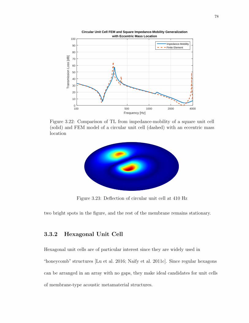
78

Frequency [Hz]100 500 1000 2000 4000

Tra

nsm

issi

on L

oss

[dB

]

0

10

20

30

40

50

60

70

80

90

100

Circular Unit Cell FEM and Square Impedance-Mobility Generalizationwith Eccentric Mass Location


Figure 3.22: Comparison of TL from impedance-mobility of a square unit cell(solid) and FEM model of a circular unit cell (dashed) with an eccentric masslocation

Figure 3.23: Deflection of circular unit cell at 410 Hz

two bright spots in the figure, and the rest of the membrane remains stationary.

3.3.2 Hexagonal Unit Cell

Hexagonal unit cells are of particular interest since they are widely used in

“honeycomb” structures [Lu et al. 2016; Naify et al. 2011c]. Since regular hexagons

can be arranged in an array with no gaps, they make ideal candidates for unit cells

of membrane-type acoustic metamaterial structures.

79

To model the waveguide, a hexagonal prism is created by extruding a hexagon

into three-dimensions. A two-dimensional shell structure models the membrane and

attached mass. To maintain an equal unit cell surface area in comparing the

hexagon to a square, the hexagon side length is calculated as

a =

√2LxLy

3√

3. (3.1)

Frequency [Hz]100 500 1000 2000 4000

Tra

nsm

issi

on L

oss

[dB

]

0

10

20

30

40

50

60

70

80

90

100Hexagonal Unit Cell FEM and Square Impedance-Mobility Generalization

Impedance-Mobility (square)Finite Element (hexagon)

Figure 3.24: Comparison of TL from impedance-mobility of a square unit cell(solid) and FEM model of a hexagonal unit cell (dashed)

The results of the FEM model of a hexagonal unit cell in a waveguide are

shown in Figure 3.24. There is good agreement between TL obtained using the

impedance-mobility approach for a square unit cell of equal area and with FEM.

There is some discrepancy in the frequencies of the first resonance at 220 Hz and TL

peak at 340 Hz with relative errors of less than 3% and 5%, respectively. The

second resonance at 3510 Hz is more accurately captured with relative error of

approximately 1%.

80

Frequency [Hz]100 500 1000 2000 4000

Tra

nsm

issi

on L

oss

[dB

]

0

10

20

30

40

50

60

70

80

90

100

Hexagonal Unit Cell FEM and Square Impedance-Mobility Generalizationwith Eccentric Mass Location


Figure 3.25: Comparison of TL from impedance-mobility of a square unit cell(solid) and FEM model of a hexagonal unit cell (dashed) with an eccentric masslocation

Figure 3.25 shows the effect of an eccentric mass location on the hexagonal

unit cell, compared to the TL of a square unit cell. The mass is located 3 mm

off-center toward the an edge of the hexagon so that it is affected by the symmetric

vibration modes of the membrane. There is an additional resonance and TL peak at

approximately 420 Hz due to the rotary inertia of the attached mass, as depicted in

Figure 3.26. At this frequency the attached mass rotates independently of the

membrane. The unit cell as a whole does not couple to the surrounding fluid well

since there is no net volume displacement at the 420 Hz resonance.

3.3.3 Triangular Unit Cell

As the number of sides of a regular polygon increases, the shape approaches a circle.

Having established that the impedance-mobility model of a square unit cell

approximates the TL of a circular unit cell, it follows that it will also approximate

81

Figure 3.26: Deflection of hexagonal unit cell at 420 Hz

regular polygons with four or more sides. This is proven in the previous section with

the study of a hexagonal unit cell. To thoroughly investigate the effect of unit cell

shape, decreasing the number of sides to three is also necessary. An equilateral

triangular unit cell is modeled using an acoustic-shell interaction FEM model to

complete the study of unit cell shape and its effect on TL.

The side length of an equilateral triangle necessary to maintain the same area

as the square unit cell is given by

a =

√4LxLy√

3. (3.2)

The model of a waveguide is created by extruding an equilateral triangle into the

z-direction. The same initial and boundary conditions as the previous cases of

rectangular, circular, and hexagonal geometries are used for the triangular

configuration.

The results plotted in Figure 3.27 show moderate agreement between the two

models. The impedance-mobility model underestimates the TL by approximately 3

dB over the frequency range of interest, with the exception of between the first

82

Frequency [Hz]100 500 1000 2000 4000

Tra

nsm

issi

on L

oss

[dB

]

0

10

20

30

40

50

60

70

80

90

100Triangular Unit Cell FEM and Square Impedance-Mobility Generalization


Figure 3.27: Comparison of TL from impedance-mobility of a square unit cell(solid) and FEM model of a triangular unit cell (dashed)

resonance and TL peak. The TL peak at 370 Hz differs by less than 4% between the

models. The first and second resonance frequencies have relative errors of

approximately 6% at 240 Hz and 11% at 4000 Hz, respectively.

Frequency [Hz]100 500 1000 2000 4000

Tra

nsm

issi

on L

oss

[dB

]

0

10

20

30

40

50

60

70

80

90

100

Triangular Unit Cell FEM and Square Impedance-Mobility Generalizationwith Eccentric Mass Location


Figure 3.28: Comparison of TL from impedance-mobility of a square unit cell(solid) and FEM model of a triangular unit cell (dashed) with an eccentric masslocation

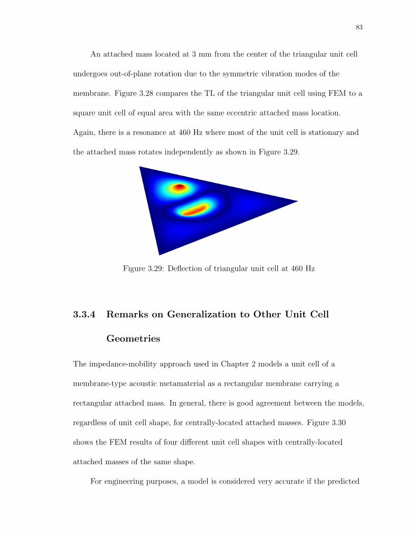
83

An attached mass located at 3 mm from the center of the triangular unit cell

undergoes out-of-plane rotation due to the symmetric vibration modes of the

membrane. Figure 3.28 compares the TL of the triangular unit cell using FEM to a

square unit cell of equal area with the same eccentric attached mass location.

Again, there is a resonance at 460 Hz where most of the unit cell is stationary and

the attached mass rotates independently as shown in Figure 3.29.

Figure 3.29: Deflection of triangular unit cell at 460 Hz

3.3.4 Remarks on Generalization to Other Unit Cell

Geometries

The impedance-mobility approach used in Chapter 2 models a unit cell of a

membrane-type acoustic metamaterial as a rectangular membrane carrying a

rectangular attached mass. In general, there is good agreement between the models,

regardless of unit cell shape, for centrally-located attached masses. Figure 3.30

shows the FEM results of four different unit cell shapes with centrally-located

attached masses of the same shape.

For engineering purposes, a model is considered very accurate if the predicted

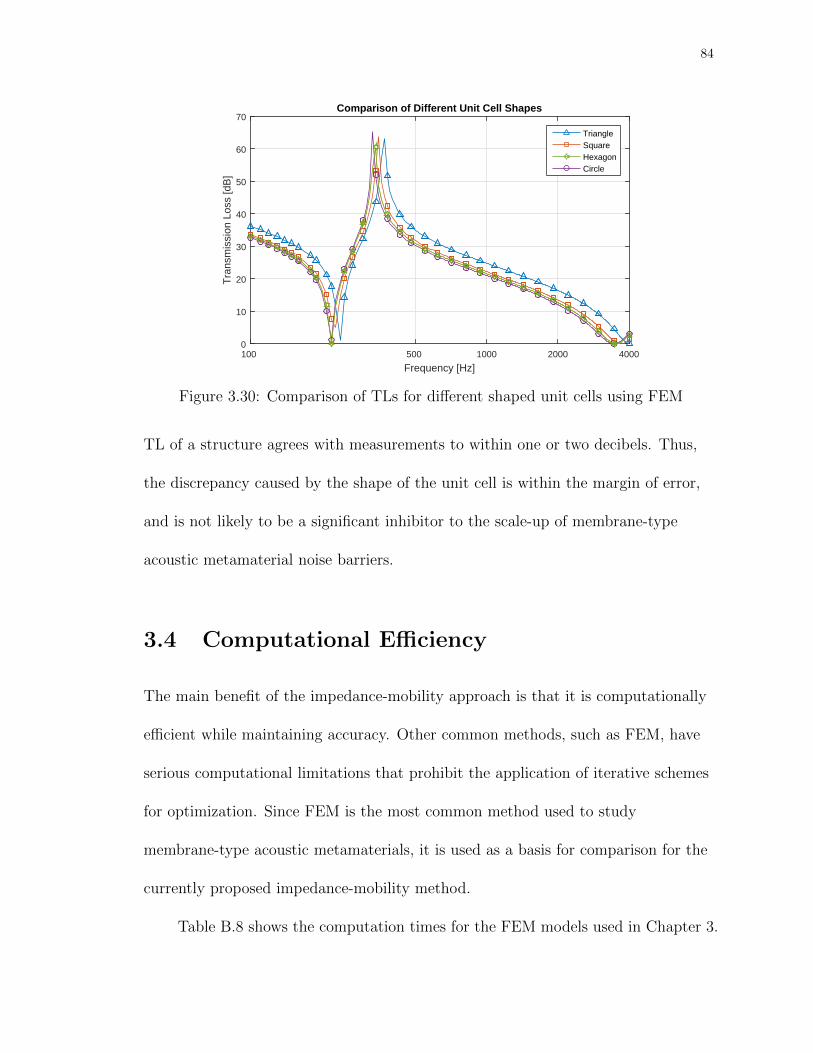
84

Frequency [Hz]100 500 1000 2000 4000

Tra

nsm

issi

on L

oss

[dB

]

0

10

20

30

40

50

60

70Comparison of Different Unit Cell Shapes

TriangleSquareHexagonCircle

Figure 3.30: Comparison of TLs for different shaped unit cells using FEM

TL of a structure agrees with measurements to within one or two decibels. Thus,

the discrepancy caused by the shape of the unit cell is within the margin of error,

and is not likely to be a significant inhibitor to the scale-up of membrane-type

acoustic metamaterial noise barriers.

3.4 Computational Efficiency

The main benefit of the impedance-mobility approach is that it is computationally

efficient while maintaining accuracy. Other common methods, such as FEM, have

serious computational limitations that prohibit the application of iterative schemes

for optimization. Since FEM is the most common method used to study

membrane-type acoustic metamaterials, it is used as a basis for comparison for the

currently proposed impedance-mobility method.

Table B.8 shows the computation times for the FEM models used in Chapter 3.

85

For each model a frequency range of 100 Hz to 4000 Hz is used with a spacing of 10

Hz for a total of 391 frequency points. The fastest run time of 1 minute and 39

seconds is achieved with a 2D axi-symmetric model which only considers a circular

unit cell with a centrally-located cylindrical attached mass. In some cases this

model can accurately estimate of TL of a square unit cell, as shown in Figure 3.20.

The slowest run time of 17 hours and 5 minutes is experienced with the most

realistic model which considers the finite thickness of the membrane and attached

mass in three dimensions.

The computational efficiency of the impedance-mobility approach arises from

its compact matrix formulation, and the opportunistic application of

simply-supported boundary conditions and rectangular geometry. Those choices

enable the integrals formulated in Chapter 2 to be evaluated explicitly and

hard-coded so that no numerical integration is needed within the program.

Appendix E shows the evaluation of the integrals.

The impedance-mobility model running on the same machine as the FEM

models using the same frequency range and spacing executes in less than 0.1

seconds. This corresponds to an increase in speed of nearly 100,000% over the

fastest FEM model.

The exceptional computational efficiency of the impedance-mobility approach

for membrane type acoustic metamaterials enables the use of iterative optimization

schemes such as genetic algorithms. Additionally, the proposed model is well-suited

to implementation in user-friendly tools for design. A graphical user interface

(GUI), is used as a front-end to the impedance-mobility model formulated in

86

Chapter 2 that allows a user to alter the design parameters of a unit cell, and at the

click of a button view its TL response.

Figure 3.31: Graphical user interface for single and double layer unit cells in awaveguide

Figure 3.31 shows the GUI created in MathWorks MATLAB 2014b. The GUI

allows the user to select between a single unit cell and a double layer of unit cells

that are defined independently. In addition to being user-friendly, the GUI is also

portable since it is compiled as an executable file. The file requires MATLAB

Runtime to operate, which is freely available on the MathWorks website

[MathWorks 2016].


This chapter presents the verification of the impedance-mobility models formulated

in Chapter 2, the validation of assumptions made in the models, and generalization

87

of the models of square unit cells to other geometries.

The TL of a single unit cell in a waveguide and a baffle calculated from the

impedance-mobility models is compared to the TL from corresponding FEM

models, with good agreement. The same is done for double layers of unit cells in a

waveguide and 2×1 and 2×2 arrays in a baffle, with the same high degree of

accuracy. A decrease in accuracy is noted at high frequencies for arrays of unit cells.

This corresponds to the breakdown of the assumption that the unit cells behave as

ideal elementary piston-like radiators.

Through manipulation of the FEM models to match the constraints used in the

impedance-mobility approach, the assumptions of negligible bending stiffness and

rotary inertia in the attached mass are tested. The bending stiffness of the attached

mass does not significantly impact the TL of a single unit cell in a waveguide. By

moving the attached mass off-center and varying its thickness, the effect of rotary

inertia is tested. The out-of-plane rotation of the attached mass results in a

resonance and TL peak at a specific frequency corresponding to the thickness of the

attached mass and its location. The impedance-mobility approach accurately

predicts TL away from this additional resonance.

By comparing the TL of a square unit cell to circular, hexagonal, and

triangular unit cells of equivalent area, the degree to which the impedance-mobility

approach can be used to predict the TL of different geometries is studied. The

impedance-mobility model of a square unit cell of a membrane-type acoustic

metamaterial with a centrally-located mass accurately predicts the TL of hexagonal

and circular unit cells. Attached mass eccentricity degrades the predictive accuracy

88

of the model near the resonance corresponding to out-of-plane rotation of the

attached mass. The TL of triangular unit cells is predicted substantially less

accurately than those of hexagonal or circular geometries. However, for

regular-polygonal unit cells with centrally-located attached masses, the

impedance-mobility accurately predicts TL.

In designing membrane-type acoustic metamaterial noise barriers, the shape of

the unit cell can be determined by external factors, such as ease of fabrication. For

regular-polygonal unit cell shapes with centrally-located attached masses, the

impedance-mobility model of a square unit cell with an equivalent area can be used

to accurately predict the TL response.

In addition to being accurate, the impedance-mobility model is also

computationally efficient. This enables optimization using genetic algorithms which

is presented in Chapter 4, and the formulation of tools for design such as the GUI

shown in this chapter.

89

Chapter 4

Optimization Using Genetic Algorithms

Determining the transmission loss (TL) of membrane-type acoustic

metamaterial noise barriers involves many design parameters that are often

inter-connected. In fact, the TL for a single unit cell set in a waveguide formulated

in Chapter 2 is a function of thirteen distinct variables. For a configuration of two

unit cells arrayed in a baffle or layered in series, that number more than doubles.

Additionally, each variable can take any value, which creates an infinite number of

possible unit cell configurations. As discussed in the introductory chapter, an

exhaustive search for an optimal design is not computationally possible, or

practically feasible.

To optimize the performance of a unit cell to meet specific design criteria, a

genetic algorithm (GA) is applied. A GA is a global optimization method that

iteratively improves each set of candidate solutions, or generation, by using

information from past generations. Characteristics of high-performing candidate

solutions are passed on to the next generation. GAs are especially well-suited to

90

problems, such as the one at hand, that contain many variables and/or nonlinear

fitness functions. The flowchart in Figure 1.5 describes the basic GA process.

This chapter explores the implementation of GAs to optimize the TL of

membrane-type acoustic metamaterial unit cells. Each step of the GA is discussed,

focusing on how they are implemented in this research. A variety of noise source

spectra and corresponding fitness functions used to design optimal configurations of

membrane-type acoustic metamaterial unit cells to control them are presented.

Results of a selection of case studies are presented in Chapter 5 to illustrate the

usefulness of GAs for design problems.

4.1 Design Variables

The design variables that determine the unique TL response of the unit cell, and the

fitness of a candidate solution, can either be continuous or discrete. Continuous

variables can take any value inside of a specified range, whereas discrete variables

are chosen from a finite set of possibilities. Genetic algorithms are inherently

well-suited for optimizing fitness functions that include any combination of

continuous or discrete variables. To shed light on the connections between design

variables the GA is performed twice, once with the assumption that all design

variables are continuous, and again assuming that there is a finite set of materials

from which the substructure can be fabricated.

For the specific case of membrane-type acoustic metamaterials, the thirteen

design variables are defined in Table 4.1, and are free to take values in the specified

91

Table 4.1: Design variable ranges

Parameter Symbol Units Minimum MaximumUnit cell width Lx mm 15 35Unit cell height Ly mm 15 35Membrane thickness tmem mm 0.0125 0.1506Membrane density ρmem kg/m3 900 2500Membrane tension T N/m 50 500Membrane elastic modulus E GPa 0.0008 5Membrane Poisson’s ratio ν - 0.3 0.5Mass density ρmass kg/m3 1000 20000Mass thickness tmass mm 1.5 6Mass width ratio lx,r - 0.01 0.25Mass height ratio ly,r - 0.01 0.25Mass x location ratio x0,r - 0.0625 0.5Mass y location ratio y0,r - 0.0625 0.5

ranges. These values are carefully chosen to ensure that randomly generated

configurations are physically viable. For example, the membrane thickness is limited

to a range in which most commercially available materials lie. The membrane

properties are limited to ranges that encompass densities, elastic moduli, and

Poisson’s ratios of materials that are likely to be used (see Table B.4). The applied

tension is limited such that the resultant stress is not likely to cause failure of the

material.

It is probable that a manufacturer may only be able to choose from a finite set

of materials, unit cell sizes, or mass sizes. In this case the discrete form of the GA

or a combination of continuous and discrete can be used to optimally design unit

cell configurations. The possible membrane and mass materials used in this

research, are listed in Tables B.4 and B.5, respectively. Possible mass sizes are given

in Table B.6. Notice that the number of materials and mass sizes in the selected sets

are powers of two, which facilitates the conversion of the binary string to represent a

92

material number or mass size. For numbers that are not powers of two, some other

encoding/decoding scheme is necessary to convert between material identifier and

binary representation.

4.2 The Population

In GAs the set of candidate solutions to the optimization problem is called the

population. The population changes and improves over time with each new

generation. The candidate solutions in a population are represented by binary

strings called chromosomes, which are subdivided into genes as shown in Figure 4.1.

The genes are then decoded into a set of input variables for the fitness function.

The initial population is a randomly generated set of chromosomes.

Chromosome︷︸︸︷1010010︸︷︷︸Gene1

1010110︸︷︷︸Gene2

1011101︸︷︷︸Gene3

. . .

Figure 4.1: Chromosome representation

To assess the performance of a candidate solution, the representative

chromosome must first be decoded into a set of input variables. A binary string of

B bits can be converted to an integer via the equation

Int =B∑

i=1

Bin(B − i+ 1) · 2i−1, (4.1)

where Bin is the binary string corresponding to a gene and its argument is the bit

location ranging from 1 to B. Once an integer value, Int, is obtained, the result can

93

be used directly as a representative for a discrete set of variables, as in the case for

selecting one component over another. Alternatively, the integer can be scaled to fit

the range of values that a parameter, x, can take by specifying a minimum and

maximum value, xmin and xmax respectively, and applying the equation

x = xmin +xmax − xmin

2B − 1Int. (4.2)

In this research seven bits per gene are used to represent the range of possible

values for each design variable. This results in 128 different design variable values in

the specified ranges, which adequately sample the range of possible values for each

parameter. Increasing the number of bits per gene increases the density of variable

values and exploration of the search space, while decreasing computational

efficiency. Design variables that require a more detailed search can use more bits in

the encoding/decoding process resulting in a finer resolution. For the case of

optimizing a single unit cell set in a waveguide, the chromosome representing a

unique solution is (13× 7 =) 91 bits in length.

4.3 Fitness Functions

The fitness score of each candidate solution is a measure of its performance by

which it is ranked against other solutions. The GA attempts to maximize this score.

It is the job of the noise control engineer to create a fitness function that adequately

defines the goal of the noise barrier for a given task.

94

This section describes several types of scenarios that noise control engineers

may encounter, and how GAs can be applied to create treatment using

membrane-type acoustic metamaterials. Developing fitness functions for broadband

noise, noise focused in a single octave band or one-third octave band, discrete

frequency noise, and noise with multiple discrete frequency components is discussed.

This section is not intended to be a panacea for the design of noise control

solutions via GAs, but to serve as a guide to address some common scenarios. Each

unique situation will require careful thought to fully characterize a successful

treatment, and to formulate a metric that quantifies the degree of success. The

fitness functions outlined below for common scenarios may serve as a good starting

point to create fitness functions for specific cases.

4.3.1 Broadband

In many noise control scenarios, the character of the noise source is unknown or is

known to vary greatly in level and/or spectrum. The spectrum of the noise source

may also be broadband in nature, such as the one shown in Figure 4.2. In these

cases, it is often necessary to design a noise barrier that works well over a wide

range of frequencies.

To maximize broadband transmission loss of the unit cell over a finite range,

the average transmission loss over that range, given by Equation (4.3), can be used

as the fitness function. Here Fj is the fitness score of the jth candidate solution, and

95

Frequency [Hz]100 500 1000 2000 4000

Sou

nd P

ress

ure

Leve

l [dB

re

20µ

Pa]

-10

0

10

20

30

40

50

60

70

80

90Example Noise Source Spectrum

Figure 4.2: Example of predominately broadband sound pressure level spectrumof HVAC equipment

ωmax and ωmin are the highest and lowest frequencies of interest, respectively.

Fj =

∫ ωmaxωmin

TL(ω)dω

ωmax − ωmin(4.3)

In this research, the frequency range of interest is 100 Hz to 4000 Hz.

4.3.2 Narrow Band

Similarly, noise sources with a large portion of their energy in a smaller range of

frequencies can be characterized using the fitness function given by Equation 4.3 by

altering the maximum and minimum frequencies of interest. An example of this

type of noise spectrum is shown in Figure 4.3.

A special case of noise characterization in narrow bands that is particularly

interesting to engineers is octave band levels. Some measurement equipment will

only report values in octave or third-octave band levels, thus it is useful to design

96

Frequency [Hz]100 500 1000 2000 4000

Sou

nd P

ress

ure

Leve

l [dB

re

20µ

Pa]

-10

0

10

20

30

40

50

60

70

80


Figure 4.3: Example sound pressure level spectrum of HVAC equipment withhigh level in the 250 Hz octave band, which is delineated by the dotted lines

noise control solutions using the same bands. The frequency limits for octave and

third-octave bands are given in ANSI S1.11 [2004].

In this manner, the TL of a membrane-type acoustic metamaterial unit cell can

be maximized in the octave band that contains the most noise energy. For the

example in Figure 4.3, the octave band centered around 250 Hz contains the most

energy, therefore the upper and lower limits of Equation (4.3) should be set to 355

Hz and 177 Hz, respectively, to maximize TL in that band. These limits are

delineated by the vertical dotted lines in the figure.

In the same manner that fitness scores for octave bands can be obtained,

one-third octave bands can also be used. If a noise source’s spectrum is only known

in one-third octave bands, such as the case shown in Figure 4.4, it is appropriate to

devise an optimization scheme based on the same band structure.

In this scenario, designing a noise barrier to optimally reduce the sound level in

97

Center Frequency [Hz]100 125 160 200 250 315 400 500 630 800 1000 1250 1600 2000 2500 3150 4000

Sou

nd P

ress

ure

Leve

l [dB

re

20 µ

Pa]

0

10

20

30

40

50

60

70

80

90

100Third Octave Band Sound Pressure Level

Figure 4.4: Third octave band sound pressure level of water-cooled screw chiller

the 315 Hz one-third octave band can be accomplished by using Equation (4.3) with

frequency limits of 282 Hz and 355 Hz as a fitness function.

4.3.3 Discrete Frequency

Equipment with rotating or oscillating elements often emit noise primarily at

frequencies determined by the speed of rotation. In this situation, it may be

desirable to design a noise barrier that has its maximum transmission loss at the

problem frequency. For this specific application, the transmission loss can be used

as the fitness score directly. Finding the optimal configuration to attenuate a tone

can be accomplished using the fitness function

Fj = TL(ω0), (4.4)

where ω0 is the frequency of the tone.

98

Figure 4.5 shows an example of noise with a prominent tone at 613 Hz. To

Frequency [Hz]100 500 1000 2000 4000

Sou

nd P

ress

ure

Leve

l [dB

re

20µ

Pa]

-10

0

10

20

30

40

50

60

70

80


Figure 4.5: Example of a noise source spectrum containing a prominent tone

design a membrane-type acoustic metamaterial unit cell with TL peak frequency

coincident with the problematic tone, the fitness function given by Equation (4.4) is

used. In the example shown, the argument ω0 is set to 613 Hz.

4.3.4 Multiple Discrete Frequencies

Similarly, attenuating a noise source comprised of one or more tones can be

accomplished using a fitness function that is a linear combination of the

transmission loss at the frequencies of interest as follows,

Fj =N∑

n=1

anTL(ωn), (4.5)

where TL(ωn) is the transmission loss at the nth frequency of interest and an is its

respective (real and positive) weighting factor. Using this fitness function allows the

99

noise control engineer to assign priority to the most problematic tones, while still

addressing tones that may be less troublesome.

For a noise source that contains multiple discrete frequency tones, such as that

in Figure 4.6, an engineer may want to design a membrane-type acoustic

metamaterial noise barrier that will consider the frequency and relative amplitudes

of the tones in the example.

Frequency [Hz]100 500 1000 2000 4000

Sou

nd P

ress

ure

Leve

l [dB

re

20µ

Pa]

-10

0

10

20

30

40

50

60

70

80


Figure 4.6: Example of a noise source spectrum containing multiple tones

To do this, the fitness function given by Equation (4.5) can be used with

component weights shown in Figure 4.7. The most prominent tones are weighted

more heavily than the others, resulting in a fitness function that prioritizes design

criteria.

4.3.5 Mass Law

In addition to the TL of the unit cell, the total weight may also be an important

design criterion. In the analysis of membrane-type acoustic metamaterial noise

100

Frequency [Hz]100 500 1000 2000 4000

Com

pone

nt W

eigh

t

0

0.2

0.4

0.6

0.8

1

Fitness Function Component Weights

Figure 4.7: Example of component weights for a fitness function

barriers, the mass law is the standard by which performance is often gauged. The

mass law, Equation (1.1), gives the TL of a thin limp panel of infinite extent and

surface density ρs. For every doubling of mass, or surface density, the mass law TL

will increase by approximately 6 dB.

The fitness functions derived in the previous sections can be altered so that the

increase in TL above the mass law is the quantity considered. This will prevent the

GA from simply adding mass to a unit cell to improve its TL. To do this the

transmission loss due to the mass law can be subtracted from the TL of the

membrane-type acoustic metamaterial unit cell, before being used in the fitness

function. Equations (4.3) - (4.5) can be re-written to account for the mass of the

unit cell as

Fj =

∫ ωmaxωmin

TL(ω)− TLm(ω)dω

ωmax − ωmin, (4.6)

101

Fj = TL(ω0)− TLm(ω0), (4.7)

and

Fj =N∑

n=1

an (TL(ωn)− TLm(ωn)) , (4.8)

respectively, where TLm is the mass law transmission loss.

Since fitness-proportionate selection, which is described in the next section,

requires fitness function values to be real and positive, negative values of Fj are

rounded up to zero. This ensures that the probability at which each candidate

solution is selected can be computed. Additionally, it guarantees that candidate

solutions with fitness function values of zero or less will not be selected.

4.4 Selection, Crossover, and Mutation

The heart of the GA is the set of processes that mimic natural selection and

Darwinian evolution. “Survival of the fittest” dictates that attributes of

higher-performing chromosomes will be passed on to future generations due to

selection. The combination of these attributes occurs through the process of

crossover. Mutation introduces genetic diversity into the population by randomly

altering a chromosome. This section details the parameters of each process used in

the design of optimal unit cells of membrane-type acoustic metamaterials.

Selection is the process by which candidate solutions are chosen to pass on

their characteristics to the next generation. In this research a combination of elite

102

selection and fitness-proportionate selection is used. In elite selection, a certain

number of the top-performing candidate solutions are chosen to proceed. This

guarantees that the best-performing candidates in any given generation survive and

pass on their genetic material. In addition to ensuring that superior genes are

passed on, it also ensures that each subsequent generation’s top performing

candidate is at least as fit as the previous generation’s. In fitness-proportionate

selection, chromosomes are selected with a probability based on their fitness scores

given by Equation (1.21).

In this research, the two most fit candidate solutions out of a total of 96 per

generation are chosen via elite selection. To keep the number of candidate solutions

in each generation constant, 94 chromosomes are chosen using fitness-proportionate

selection. It is possible that some, most likely higher-performing, candidate

solutions are chosen multiple times. The 94 selected chromosomes then move on to

swap genetic information via crossover, creating 94 new chromosomes that are

added to the two elite chromosomes to create the new generation.

Crossover is the process by which genetic information from two chromosomes is

combined to create new chromosomes. The most common form, and what is used in

this research, is single-point crossover. In this scheme a random point in the

chromosome is chosen and the bits to the left of that point from one chromosome

and to the right of that point in another, and vice-versa, are combined to make two

new chromosomes. Additionally, maximum-minimum crossover is used which

sequentially pairs the most and least fit chromosomes for crossover. This creates

more genetic diversity by mixing attributes of high-performing candidates with

103

those of low-performing ones.

Mutation randomly introduces additional genetic diversity by changing a

random bit in a gene from a one to a zero or vice versa. The probability at which

mutation occurs is set at µ = 0.1 in this research to introduce more genetic material

into the population. To ensure that each generation improves upon the last or at

least remains the same, the highest performing solution is immune from mutation.

4.5 Convergence

The stopping criteria of the GA determine when an optimal solution has been

reached. Convergence is reached when the best chromosome, and its fitness score,

remains unchanged for many generations. For this research, the GA stops when a

particular candidate solution has the highest fitness score for ten consecutive

generations. Figure 4.8 shows an example of GA convergence. The maximum,

average, and minimum fitness scores in each generation are shown. Notice that the

maximum fitness score increases or remains constant with each subsequent

generation, ensuring convergence. The minimum fitness score, representing the least

fit candidate solution, varies wildly due to the introduction of new genetic material

through mutation. If the GA fails to converge on an optimal solution, the GA is

stopped when the number of generations reaches a predefined limit, set to 200 in

this research so that the algorithm is likely to converge.

The GAs were implemented using custom scripts in MathWorks MATLAB

2015a and computed on a Windows PC with an Intel Core-i5 3.4 GHz processor and

104

Generation Number5 10 15 20 25 30 35 40 45 50 55 60

Fitn

ess

Sco

re [d

B]

0

10

20

30

40

50

60

70GA Convergence

Figure 4.8: Example of GA convergence. Generation maximum (red solid),average (dotted), and minimum (blue solid) fitness score.

16 gigabytes of RAM. In the example shown in Figure 4.8, convergence was reached

in 60 generations, resulting in (60×96=) 5760 evaluations of unit cell TL using the

impedance-mobility approach. The process took 20 minutes and 17 seconds. The

same GA using a FEM model as described in Chapter 3 to evaluate the fitness of

each candidate solution would take 592 days to complete. See Table B.8 for further

information on the efficiency of FEM models. Implementing a GA would not be

feasible without the computationally efficient models developed in Chapter 2.


This chapter presents the application of genetic algorithms to find optimal

configurations of membrane-type acoustic metamaterials. Fitness functions were

developed to maximally attenuate broadband, narrow band, discrete frequency, and

multiple discrete frequency component noise. Each step in the GA is discussed,

105

focusing on how they are implemented in this research. The stopping criteria and

convergence are noted. Chapter 5 presents the results of the GAs applied to the TL

from the impedance-mobility formulation of a unit cell of a membrane-type acoustic

metamaterial in a waveguide using each of the fitness functions described in this

chapter.

106

Chapter 5

Results

This chapter is divided into two sections. The first section presents the results

of studies conducted using the impedance-mobility models formulated in Chapter 2

and verified in Chapter 3. Design variables are manipulated independently to show

their effect on the transmission loss of a unit cell, cell arrays, and double layers of

unit cells. This serves to illustrate the myriad possible configurations and resulting

TL profiles, and informs the necessity of an optimization scheme.

The second section presents the results of genetic algorithm optimization using

the fitness functions developed in Chapter 4. By simultaneously altering each design

parameter and iteratively improving the unit cell configuration, the GA eliminates

the otherwise arduous process of design. The GAs are applied to each scenario three

times, once with each design variable free to take a value within its specified range,

again using a fitness function that accounts for the total weight of the unit cell, and

yet again with a limited selection of materials available. The design variable ranges

are given in Table B.3, and the selected materials are given in Tables B.4 - B.7.

107

5.1 Impedance-Mobility Model

5.1.1 Single Unit Cell

To understand the impact that each design variable has on the transmission loss of

the structure, the impedance-mobility model is used to study its deviation from a

baseline configuration of a single unit cell in a waveguide. The parameter values

used for the baseline configuration are given in Table B.1, and the corresponding

transmission loss is shown in Figure 5.1.

Frequency [Hz]100 500 1000 2000 3000 4000

Tra

nsm

issi

on L

oss

[dB

]

0

10

20

30

40

50

60

70

80

90

100Single Layer Transmission Loss

Figure 5.1: TL of unit cell with baseline parameters given in Table B.1

There are three main parts of the TL curve that will be discussed in this

Chapter, two resonances and a TL peak. The first resonance for the baseline

configuration occurs at 226 Hz corresponding to maximum in-phase vibration of the

membrane and attached mass. The second resonance at 3560 Hz occurs when the

attached mass remains stationary and the membrane vibrates independently. The

TL peak occurs between these two resonances at 356 Hz, where the surface-average

108

displacement is zero, leading to perfect reflection of the incident wave. Figure D.1 in

Appendix D shows the displacement at each of these frequencies.

5.1.1.1 Waveguide vs. Baffle

It is useful from the standpoint of a noise control engineer to examine how sound is

reduced by a membrane-type acoustic metamaterial used as a partition or barrier. A

first step in doing this is considering the TL of a unit cell which radiates its energy

into a hemispherical half-space bounded by a rigid planar baffle. This simulates its

response when set in a wall or other approximately rigid surface much larger than a

unit cell. The TLs of single unit cells set in a waveguide and in a baffle are shown in

Figure 5.2.

Frequency [Hz]100 500 1000 2000 3000 4000

Tra

nsm

issi

on L

oss

[dB

]

0

10

20

30

40

50

60

70

80

90

100Single Unit Cell Waveguide vs Baffled Transmission Loss

WaveguideBaffle

Figure 5.2: Comparison of TL of unit cell in a waveguide (solid) and a baffle(dashed)

The baffled TL is approximately 40 dB greater than that of the waveguide

below the first resonance frequency, and 30 dB higher at the TL peak frequency. As

109

the frequency increases, the TL approaches that of a unit cell in a waveguide.

The higher TL that is seen with an identical unit cell set in a baffle is easily

explained by examining the modal radiation efficiency for a simply supported panel.

Figure A.3 in Appendix A shows that the radiation efficiency for each mode

increases as a function of frequency. This means that at low frequencies, the

vibratory motion of the unit cell does not couple well with the surrounding fluid. In

a waveguide the radiated sound propagates as a plane wave and the unit cell

effectively behaves as a rigid piston, which has unity radiation efficiency, leading to

a maximum transmitted sound power and minimum TL. The TL of a unit cell in a

waveguide can thus be treated as the lower limit of TL obtainable by an ideal

membrane-type acoustic metamaterial unit cell.

5.1.1.2 Angle of Incidence

For a finite plate or membrane in a rigid baffle, the angle of incidence can influence

the transmission loss when the trace wavelength of the incident wave matches that

of the panel. The angle of incidence is explored using Equation (E.12) for the

generalized modal force acting on the unit cell. For a membrane-type acoustic

metamaterial, there is little effect of varying incidence angle due to the small

dimensions of the unit cell since ka� 1, where ka is the dimensionless spatial

frequency parameter. This is shown in Figure 5.3, where there is less than 1 dB of

change between normally and obliquely (α = 78◦, β = 78◦) incident excitation from

2000 Hz to 4000 Hz. Here α and β are the angles from the normal vector of the unit

cell in the x and y directions, respectively. There is practically no difference in TL

110

at lower frequencies.

Frequency [Hz]2000 3000 4000

Tra

nsm

issi

on L

oss

[dB

]

0

5

10

15

20

25

30Single Unit Cell Baffled Transmission Loss

Normally Incidentα = 78°, β = 78°

Figure 5.3: Comparison of TL of unit cell in a baffle for normally incident (solid)and obliquely incident (dashed) excitation

5.1.1.3 Membrane Tension

The resonance frequencies of an unloaded membrane of dimensions (Lx × Ly) are

given by the equation

ωm =

√T

ρs

√(m1π

Lx

)2

+

(m2π

Ly

)2

, (5.1)

where m1 and m2 are the mode numbers in the x and y directions, respectively. It is

evident that the resonance frequencies are proportional to the square root of the

tension, T , and it follows that the TL peak frequency is also proportional to the

square root of the tension. Figure 5.4 shows the effect of increasing the tension

applied to the membrane. The first and second resonances as well as the TL peak

shift toward higher frequencies with increasing tension.

111

Frequency [Hz]100 500 1000 2000 3000 4000

Tra

nsm

issi

on L

oss

[dB

]

0

10

20

30

40

50

60

70

80

90


T = 3 MPaT = 4 MPaT = 5 MPaT = 6 MPa

Figure 5.4: TL of unit cell with varied tension

5.1.1.4 Membrane Surface Density

According to Equation (5.1) the unloaded resonance frequencies of the membrane

are proportional to 1/√ρs. However, the first resonance frequency of the loaded

membrane is negligibly affected by variations in the membrane surface density due

to the presence of the attached mass. At the first resonance, the unit cell behaves

similarly to a simple harmonic oscillator. At the second resonance frequency, the

unit cell is maximally affected by variations in the membrane surface density since

at this resonance the attached mass is stationary and does not affect the unit cell

vibration. These phenomena are observed in Figure 5.5, where increasing the

surface density of the membrane negligibly affects the first resonance and TL peak

frequencies while decreasing the second resonance frequency.

112

Frequency [Hz]100 500 1000 2000 3000 4000

Tra

nsm

issi

on L

oss

[dB

]

0

10

20

30

40

50

60

70

80

90


ρmem

= 900 [kg/m3]

ρmem

= 1200 [kg/m3]

ρmem

= 1500 [kg/m3]

ρmem

= 1800 [kg/m3]

Figure 5.5: TL of the unit cell with varied membrane density

5.1.1.5 Membrane Stiffness

As illustrated in Section 2.1.2, the stiffness of a vibrating membrane is sometimes

neglected in analytical models. To illustrate its importance, the impedance-mobility

model is used to compare the TL of a unit cell in a waveguide with and without

bending stiffness. Figure 5.6 shows the TL of a baseline unit cell with tension and

stiffness (solid), tension only (dashed), and stiffness only (dotted).

It is evident that tension plays a much larger role in the TL of the unit cell.

However, stiffness does affect the TL peak frequency which is the most important

part of the TL profile. In the frequency range near the TL peak, the effective

dynamic mass of the unit cell is negative which can be considered the defining

characteristic of a metamaterial. It is therefore important to consider both tension

and stiffness in models of membrane-type acoustic metamaterials.

It is also necessary to examine the degree to which the membrane stiffness

113

Frequency [Hz]100 500 1000 2000 3000 4000

Tra

nsm

issi

on L

oss

[dB

]

0

10

20

30

40

50

60

70

80

90


Tension and StiffnessTension OnlyStiffness Only

Figure 5.6: Comparison of TL for both tension and stiffness (solid), tension only(dashed), and stiffness only (dotted)

influences the TL of a unit cell. The natural frequencies of an unloaded plate are

proportional to the square root of its stiffness, as shown in Equation (A.5). In the

same manner as applied tension, as the stiffness increases (i.e. the Young’s modulus

of the membrane material increases), so do the resonance and TL peak frequencies.

Frequency [Hz]100 500 1000 2000 3000 4000

Tra

nsm

issi

on L

oss

[dB

]

0

10

20

30

40

50

60

70

80

90

100Effect of Membrane Stiffness on Transmission Loss

Emem

= 0.4 GPa

Emem

= 2.4 GPa

Emem

= 4.4 GPa

Emem

= 6.4 GPa

Figure 5.7: TL of unit cell with varied membrane stiffness

114

The TL is shown in Figure 5.7 with varying degrees of membrane stiffness. As

the stiffness increases, the TL profile shifts toward higher frequencies. Increasing

stiffness also increases the magnitude of TL at the peak frequency.

5.1.1.6 Attached Mass Density

The density of the attached mass, or more accurately its magnitude, affects the first

resonance and TL peak frequency. At the first resonance, the mass and membrane

vibrate in unison, and the attached mass experiences its largest displacement. Near

this frequency, the unit cell behaves approximately as a simple harmonic oscillator,

and the resonance frequency is approximated by√k/m where k is the effective

stiffness, and m is the magnitude of the attached mass. By holding the size of the

attached mass constant, increasing its density increases the overall TL magnitude

and the first resonance frequency of the unit cell decreases.

Frequency [Hz]100 500 1000 2000 3000 4000

Tra

nsm

issi

on L

oss

[dB

]

0

10

20

30

40

50

60

70

80

90


ρmass

= 5000 [kg/m3]

ρmass

= 10000 [kg/m3]

ρmass

= 15000 [kg/m3]

ρmass

= 20000 [kg/m3]

Figure 5.8: TL of unit cell with varied density of attached mass

Figure 5.8 shows the TL for various densities of a centrally-located 3 mm × 3

115

mm × 4.5 mm attached mass. As the mass density increases, the first resonance and

TL peak frequencies decrease proportionally to√ρs. Since there is no deflection of

the attached mass at the second resonance, its frequency does not depend on mass

density.

5.1.1.7 Attached Mass Location

The location of the attached mass determines which membrane modes are

maximally affected and, in turn, the frequencies at which the TL peak and

resonances occur. To study this effect, the location of the mass is systematically

moved on a square membrane according to Figure 5.9. Because of the diagonal

symmetry of the square unit cell, only mass locations in the lower left octant need

to be explored to fully characterize the response with an arbitrary mass location.

123

4

5

x

y

Figure 5.9: Mass locations

Figures 5.10 and 5.11 show the results. As the attached mass is moved farther

from the center of the unit cell in the negative x direction, the first resonance

frequency increases and the TL peak frequency decreases due to asymmetric

116

vibration of the unit cell. Additionally, the maximum TL decreases due to the

smaller unit cell deflection at eccentric locations. At higher frequencies, addtional

resonances occur due to the asymmetric vibration of the unit cell.

Frequency [Hz]100 500 1000 2000 3000 4000

Tra

nsm

issi

on L

oss

[dB

]

0

10

20

30

40

50

60

70

80

90

100Effect of Mass Location on Transmission Loss

Location 1Location 2Location 3

Figure 5.10: TL of unit cell with varied mass location

As the attached mass location moves diagonally from the center of the

membrane, the same phenomena occur. At higher frequencies, more resonances and

TL peaks occur due to doubly-asymmetric vibration of the unit cell.

5.1.1.8 Attached Mass Size

The primary effect of changing the size of the attached mass has relatively little to

do with the mass itself. Increasing the size of the attached mass, as shown in

Figure 5.12, decreases the distance between the outer edge of the membrane and the

mass, which increases the frequency of the first resonance. This is shown in

Figure 5.13. Additionally, increasing the size of the attached mass increases the

effective density of the unit cell as a whole, which decreases the frequency of the

117

Frequency [Hz]100 500 1000 2000 3000 4000

Tra

nsm

issi

on L

oss

[dB

]

0

10

20

30

40

50

60

70

80

90

100Effect of Mass Location on Transmission Loss

Location 1Location 4Location 5

Figure 5.11: TL of unit cell with varied mass location

second resonance. The same phenomenon is seen in Figure 5.5.

1 2 3

Figure 5.12: Mass sizes

5.1.1.9 Unit Cell Aspect Ratio

The shape of the unit cell affects the spacing between the resonance frequencies of

the unloaded membrane. As the aspect ratio r = Lx/Ly increases toward one while

maintaining an equal unit cell area, the first resonance frequency associated with

118

Frequency [Hz]100 500 1000 2000 3000 4000

Tra

nsm

issi

on L

oss

[dB

]

0

10

20

30

40

50

60

70

80

90

100Effect of Mass Size on Transmission Loss

Mass Size 1Mass Size 2Mass Size 3

Figure 5.13: TL of unit cell with varied mass size

m = (1, 1) decreases. This is also true for the loaded case, and can be seen in

Figure 5.14. The second resonance of the loaded membrane occurs when the

attached mass is stationary relative to the membrane. In the unloaded case, this

corresponds to the (2, 1) or (1, 2) modes which in the case of a square, (r = 1), have

identical resonance frequencies. For aspect ratios other than one, however, the

second resonance frequency is determined by the length of the longest side. Because

of this, the second resonance frequency increases with increasing aspect ratio.

The TL peak frequency remains relatively unchanged, since the first and

second resonances are decreasing and increasing, respectively, as the aspect ratio

approaches 1.

5.1.2 Stacked Unit Cells

One method of increasing the overall TL of a membrane-type acoustic metamaterial

noise barrier is to add a second layer separated by an acoustic cavity. Using the

119

Frequency [Hz]100 500 1000 2000 3000 4000

Tra

nsm

issi

on L

oss

[dB

]

0

10

20

30

40

50

60

70

80

90


r = 0.3r = 0.5r = 0.7r = 1.0

Figure 5.14: TL of unit cell with varied aspect ratio r = Lx/Ly

impedance mobility formulation described in Section 2.3, the TL curves of a single

layer and a double layer of identical unit cells with an 8 mm air cavity in a

waveguide are shown in Figure 5.15.

Frequency [Hz]100 500 1000 2000 3000 4000

Tra

nsm

issi

on L

oss

[dB

]

0

10

20

30

40

50

60

70

80

90

100Double Layer Transmission Loss

Double with 8mm spacingMass Law

Figure 5.15: TL of a single unit cell in a waveguide (solid), and a double layerof identical unit cells with 8 mm stacking distance (dashed)

The broadband TL increases by about 10 dB, while the TL near the resonance

120

frequencies remains unchanged. An additional dip in the TL appears just above the

first resonance frequency, where the two unit cells vibrate out of phase as shown

using FEM in Figure 5.16. This corresponds to the half wavelength mass-air-mass

resonance of the effective medium formed by the two unit cells and air cavity.

Figure 5.16: Cross-section of double layer unit cell deflection at 270 Hz

5.1.2.1 Stacking Distance

The stacking distance, Lz, between two unit cells in a double layer configuration

determines the size of the acoustic cavity. This, in turn, affects the acoustic

impedance of the cavity and coupled structural mobilities of each unit cell.

The effect of varying stacking distance on the TL of a double layer of identical

unit cells in a waveguide is shown in Figure 5.17. As the stacking distance increases,

the broadband TL increases by approximately 3 dB per doubling of stacking

distance. The TL near the resonance frequencies remains unchanged.

The additional resonance introduced by the double panel configuration varies

as a function of stacking distance. The additional resonance frequency decreases

toward the first resonance as the stacking distance increases.

121

Frequency [Hz]100 500 1000 2000 3000 4000

Tra

nsm

issi

on L

oss

[dB

]

0

10

20

30

40

50

60

70

80

90

100Effect of Spacing on Double Layer Transmission Loss

Lz = 3 mm

Lz = 5 mm

Lz = 7 mm

Lz = 9 mm

Figure 5.17: TL of double layer with varied stacking distance

5.1.2.2 Different Unit Cells

The TL profile of a double layer can be manipulated by altering one or both of the

unit cells [Naify et al. 2012]. To study the effect of two different unit cells stacked in

series, an alternate configuration is established with the parameter values given in

Table B.2. The TL profiles of the individual unit cells and the double layer system

with 5 mm stacking distance are shown in Figure 5.18. As with the double layer of

identical unit cells, an approximately 10 dB overall increase in TL occurs with the

double layer system of different unit cells. Each unit cell creates a distinct TL peak

and first resonance which combine in the double layer system.

5.1.2.3 Stacking Order

Intuitively, the order in which an incident wave encounters a set of barriers could

impact the attenuation of the wave. The truth, however, is revealed by examining

Equations (2.67) - (2.69) and (2.77). In fact, the transmission coefficient is

122

Frequency [Hz]100 500 1000 2000 3000 4000

Tra

nsm

issi

on L

oss

[dB

]

0

10

20

30

40

50

60

70

80

90

100Transmission Loss of Double Layer with Different Unit Cell Configurations

Baseline ConfigurationAlternate ConfigurationStacked with 5mm spacing

Figure 5.18: TL of double layer with different unit cell configurations. Baselineconfiguration (blue solid), alternate configuration (red solid), both configura-tions stacked with 5 mm spacing (dashed)

mathematically identical regardless of stacking order. This is verified in the plot in

Figure 5.19, where the TL of two different unit cells is shown in both stacking

orders.

Frequency [Hz]100 500 1000 2000 3000 4000

Tra

nsm

issi

on L

oss

[dB

]

0

10

20

30

40

50

60

70

80

90

100Effect of Stacking Order on Transmission Loss

Baseline - AlternateAlternate - Baseline

Figure 5.19: TL of double layer with different stacking order. Baseline thenalternate configuration (solid), alternate then baseline configuration (dashed)

123

5.1.3 Multi-Cell Arrays

To study the TL of multi-cell arrays in a rigid planar baffle, the impedance-mobility

approach with the negligible coupling assumption is used. In Chapter 3 this

assumption was proven to be valid for frequencies below the second unit cell

resonance frequency. Additionally, the expansion from a single unit cell to multi-cell

array involves reducing the vibration of the unit cell to that of an equivalent

elementary radiator. To ensure that this reduction is accurate, the TL of a unit cell

in a baffle calculated using modal radiation efficiencies, and by reduction to an

elementary piston-like radiator is plotted in Figure 5.20.

Frequency [Hz]100 500 1000 2000 3000 4000

Tra

nsm

issi

on L

oss

[dB

]

0

10

20

30

40

50

60

70

80

90

100Comparison of Transmission Loss of a Baffled Unit Cell and Elementary Radiator

Impedance-MobilityElementary Radiator

Figure 5.20: TL of a baffled unit cell (solid), and an elementary radiator withequivalent average velocity (dashed)

The TL curves plotted in Figure 5.20 appear to be identical. However, at high

frequencies it is expected that there will be a reduction in accuracy due to values of

ka increasing toward 1, where ka is the dimensionless spatial frequency parameter.

This phenomenon is seen more clearly in Figure 5.21, though the discrepancy is less

124

than 1 dB at its maximum. This indicates that expansion to a multi-cell array using

equivalent elementary radiators to represent unit cells is valid below the second

resonance frequency.

Frequency [Hz]2500 3000 4000

Tra

nsm

issi

on L

oss

[dB

]

0

5

10

15

20

25Comparison of Transmission Loss of a Baffled Unit Cell and Elementary Radiator

Impedance-MobilityElementary Radiator

Figure 5.21: High frequency discrepancy between baffled unit cell (solid) andelementary radiator with equivalent average velocity (dashed)

5.1.3.1 Number of Unit Cells

As the number of unit cells in an array increases, so does the incident sound power

carried by the plane wave given by Πinc = P 2S/2ρ0c0, where P is the pressure

amplitude, S is the total surface area, and ρ0c0 is the characteristic impedance of

the fluid medium. This, however, does not lead to a change in overall TL by itself

since the velocity of each unit cell is determined by the pressure acting on it, not the

overall incident sound power. The close proximity of adjacent unit cells leads to a

doubling of radiated sound power when the number of unit cells is doubled (examine

Equation (2.55) for insight). This gives rise to an approximately 3 dB decrease in

125

TL with each doubling of total unit cells. Figure 5.22 shows the TL for a unit cell,

2× 1, 2× 2, and 3× 3 arrays in an infinite rigid baffle.

Frequency [Hz]100 500 1000 2000 3000 4000

Tra

nsm

issi

on L

oss

[dB

]

0

10

20

30

40

50

60

70

80

90

100Transmission Loss of Multi-Cellular Arrays

Unit Cell2×1 Array2×2 Array3×3 Array

Figure 5.22: Transmission loss of baffled multi-cellular arrays

For larger numbers of unit cell the reduction in TL decreases asymptotically as

the distance between adjacent unit cells increases. This is shown in Figure 5.23 for

square arrays of 4× 4, 5× 5, 6× 6, and 7× 7 identical unit cells. Note that the

negative TL at high frequencies (> 3000 Hz) is due to violation of the assumption

that the vibration pattern of a unit cell can be approximated by a piston-like

elementary radiator. The TL below approximately 2000 Hz is valid.

Because the TL decreases substantially with increasing number of unit cells,

the TL of a unit cell in a waveguide is used in Section 5.2 to design optimal

membrane-type acoustic metamaterial noise barriers. The TL of a unit cell in a

waveguide is shown (dashed) with the TLs of multi-cell arrays with large numbers of

elements in Figure 5.23. Designing ideal unit cells based on their TL in a waveguide

will give the lower limit of their performance when arrayed in a noise barrier.

126

5.1.3.2 Different Unit Cells

Another proposed method of increasing the overall TL of an array of unit cells is by

using different configurations of unit cells in the same array. Doing so results in a

TL profile that contains multiple dips and peaks corresponding to the number of

different configurations used in the array.

Figure 5.24 shows the TLs of 2× 2 arrays of baseline and an alternate

configuration unit cells in a baffle, and the TL of a 2× 2 array with two baseline

and two alternate configuration unit cells in an alternating arrangement. The TL

curve tends to take the minimum value of the two configurations. Near the TL

peaks the frequencies are shifted due to the presence of the adjacent unit cells which

have different first resonance and TL peak frequencies.

Typically, the TL of composite walls is computed using a spatially-weighted

average of the sound transmission coefficient. The dotted line in Figure 5.24,

Frequency [Hz]100 500 1000 2000 3000 4000

Tra

nsm

issi

on L

oss

[dB

]

0

10

20

30

40

50

60

70

80

90

100Transmission Loss of Multi-Cellular Arrays

4×4 Array5×5 Array6×6 Array7×7 ArrayWaveguide

Figure 5.23: Transmission loss of baffled multi-cellular arrays (solid), and asingle unit cell in a waveguide (dashed)

127

Frequency [Hz]100 500 1000 2000 3000 4000

Tra

nsm

issi

on L

oss

[dB

]

0

10

20

30

40

50

60

70

80

90

1002 x 2 Array Transmission Loss

BaselineAlternateBaseline - AlternateAverage

Figure 5.24: Transmission loss of baffled multi-cellular arrays with different unitcells. Baseline (blue solid), Alternate (red solid), combined (dashed)

however, shows that it would not be accurate in this situation due to coupling of

adjacent unit cells.

5.1.4 Mass Law

Increasing the mass of the attached mass is a good way to improve low-frequency

TL, as shown in Figure 5.8. However, doing so also increases the total weight of the

unit cell which can be undesirable in situations where weight is a critical design

criteria. The TL of the baseline configuration unit cell is plotted along with the

mass law TL of a limp panel of equivalent surface density in Figure 5.25. This shows

the increase in TL that can be gained by using membrane-type acoustic

metamaterial barriers instead of conventional materials. An improvement of more

than 40 dB is seen at the TL peak frequency; however, this improvement is confined

to a narrow band. In applying the genetic algorithms formulated in Chapter 4, the

128

Frequency [Hz]100 500 1000 2000 3000 4000

Tra

nsm

issi

on L

oss

[dB

]

0

10

20

30

40

50

60

70

80

90

100Comparison of Unit Cell Transmission Loss and Mass Law

MetamaterialMass Law

Figure 5.25: Transmission loss of single unit cell in a waveguide (solid) comparedto the mass law for a limp panel of equivalent density (dashed)

mass law TL is used as a basis of comparison for designing optimal unit cells while

maintaining a light overall weight. The mass law is typically used to characterize

the transmission loss of panels above the first panel resonance up to the coincidence

frequency, and is therefore an appropriate basis for comparison above the first

resonance frequency of a membrane-type acoustic metamaterial unit cell.

5.1.5 Derived Quantities

The quantities derived in Section 2.4 give insight into the physical phenomena that

occur when an acoustic wave impinges upon a membrane-type acoustic

metamaterial unit cell. These insights can aid the noise control engineer in

designing effective noise barriers.

129

5.1.5.1 Effective Dynamic Mass

The effective dynamic mass is a quantity that defines the operational range of

acoustic metamaterials. Anomalous spikes in TL occur when the effective dynamic

mass becomes negative, where the membrane average acceleration acts toward the

impinging wave. In this frequency range, the unit cell reflects incident energy nearly

perfectly.

Frequency [Hz]100 500 1000 2000 3000 4000

Tra

nsm

issi

on L

oss

[dB

]

0

20

40

60

80

100Effective Dynamic Mass and Transmission Loss

Effe

ctiv

e D

ynam

ic M

ass

[kg]

-0.1

-0.05

0

0.05

0.1

0.15

Transmission LossEffective Dynamic Mass

Figure 5.26: TL (solid, left axis) and effective dynamic mass (dashed, right axis)of a single unit cell in a waveguide

Figure 5.26 shows the TL and effective dynamic mass of a membrane-type

acoustic metamaterial unit cell in a waveguide calculated using Equation (2.80).

The TL peak frequency corresponds to a discontinuity in the effective dynamic

mass, where it jumps from negative to positive infinity. The resonance frequencies

occur when the effective dynamic mass is zero. As the absolute value of the effective

dynamic mass increases, the TL increases proportionally.

Similarly, a double layer of unit cells has a discontinuity in the effective

130

Frequency [Hz]100 500 1000 2000 3000 4000

Tra

nsm

issi

on L

oss

[dB

]

0

20

40

60

80

100Effective Dynamic Mass and Transmission Loss of a Double Layer

Effe

ctiv

e D

ynam

ic M

ass

[kg]

-0.1

-0.05

0

0.05

0.1

0.15

Transmission LossEffective Dynamic Mass

Figure 5.27: TL (solid, left axis) and effective dynamic mass (dashed, right axis)of a double layer of unit cells in a waveguide

dynamic mass at the TL peak frequency, where it jumps from positive to negative

and then back to positive, as shown in Figure 5.27. The effective dynamic mass also

has a value of zero at an additional frequency just above the first resonance,

corresponding to a dip in TL. Zero effective dynamic mass equates to zero net force

acting on the membrane, resulting in total reflection of the incident wave.

5.1.5.2 Reflection and Absorption Coefficients

The sound power reflection and absorption coefficients are often used to

characterized the influence on the sound field that a material has. For a

membrane-type acoustic metamaterial unit cell in a waveguide, the transmission

coefficient calculated by Equation (2.17) is used in Equations (2.81) and (2.82) to

give the reflection and absorption coefficients, respectively.

Figure 5.28 shows the sound power transmission, reflection, and absorption

131

Frequency [Hz]100 500 1000 2000 3000 4000

Ene

rgy

Coe

ffici

ents

[-]

0

0.1

0.2

0.3

0.4

0.5

0.6

0.7

0.8

0.9

1Transmission, Reflection, and Absorption

TransmissionReflectionAbsorption

Figure 5.28: Sound power transmission (solid), reflection (dashed), and absorp-tion (dotted) coefficients for a single unit cell in a waveguide

coefficients plotted against frequency. At 356 Hz the reflection coefficient goes to

one, while the transmission and absorption coefficients are zero. This corresponds to

perfect reflection of the incident wave and the TL peak seen in the transmission loss

curves. The resonance at 226 Hz corresponds to maximum displacement of the unit

cell leading to peak values of transmission and absorption coefficients of 0.25 and

0.5, respectively. Generally, the absorption coefficient increases with frequency to a

maximum value of 0.5. The transmission and reflection coefficients reach local

maxima and minima, respectively, at the resonance frequencies of 226 Hz and 3557

Hz.

The transmission, reflection, and absorption coefficients can also be calculated

for a double layer of unit cells in a waveguide as shown in Figure 5.29. The results

are similar to those of a single unit cell, with the absorption and transmission

coefficients peaking near the resonance frequencies of 226 Hz, 279 Hz, and 3622 Hz.

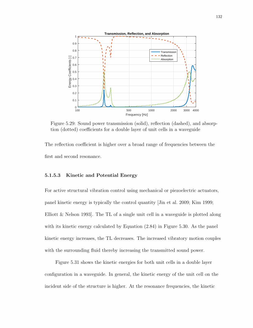
132

Frequency [Hz]100 500 1000 2000 3000 4000

Ene

rgy

Coe

ffici

ents

[-]

0

0.1

0.2

0.3

0.4

0.5

0.6

0.7

0.8

0.9

1Transmission, Reflection, and Absorption

TransmissionReflectionAbsorption

Figure 5.29: Sound power transmission (solid), reflection (dashed), and absorp-tion (dotted) coefficients for a double layer of unit cells in a waveguide

The reflection coefficient is higher over a broad range of frequencies between the

first and second resonance.

5.1.5.3 Kinetic and Potential Energy

For active structural vibration control using mechanical or piezoelectric actuators,

panel kinetic energy is typically the control quantity [Jin et al. 2009; Kim 1999;

Elliott & Nelson 1993]. The TL of a single unit cell in a waveguide is plotted along

with its kinetic energy calculated by Equation (2.84) in Figure 5.30. As the panel

kinetic energy increases, the TL decreases. The increased vibratory motion couples

with the surrounding fluid thereby increasing the transmitted sound power.

Figure 5.31 shows the kinetic energies for both unit cells in a double layer

configuration in a waveguide. In general, the kinetic energy of the unit cell on the

incident side of the structure is higher. At the resonance frequencies, the kinetic

133

Frequency [Hz]100 500 1000 2000 3000 4000

Tra

nsm

issi

on L

oss

[dB

]

0

20

40

60

80

100Unit Cell Transmission Loss and Kinetic Energy

Kin

etic

Ene

rgy

[dB

re

10-9

Jou

les]

-40

-20

0

20

Transmission LossKinetic Energy

Figure 5.30: Transmission loss (solid) and kinetic energy (dashed) of the baselineconfiguration unit cell in a waveguide

energies of both unit cells peak, which leads to a low TL.

Frequency [Hz]100 500 1000 2000 3000 4000

Kin

etic

Ene

rgy

[dB

re

10-9

Jou

les]

-60

-50

-40

-30

-20

-10

0

10Double Layer Unit Cell Kinetic Energy

Unit Cell AUnit Cell B

Figure 5.31: Kinetic energy of a double layer of baseline configuration unit cells.Panel A (solid), panel B (dashed)

The acoustic potential energy in the cavity of a double layer of membrane-type

acoustic metamaterial unit cells can be a useful quantity in active control using

acoustic secondary sources to cancel cavity modes [Jin et al. 2009; Lau & Tang

134

2006; Kim 1999; Elliott & Nelson 1993]. Figure 5.32 shows the TL of a double layer

structure and the cavity potential energy given by Equation (2.86).

Frequency [Hz]100 500 1000 2000 3000 4000

Tra

nsm

issi

on L

oss

[dB

]

0

10

20

30

40

50

60

70

80

90

100Double Layer Transmission Loss and Potential Energy

Cav

ity P

oten

tial E

nerg

y [d

B r

e 10

-12 J

oule

s]

-50

-40

-30

-20

-10

0

10

20

30

40

50

TLE

p

Figure 5.32: Transmission loss (solid) and cavity potential energy (dashed) of adouble layer of baseline configuration unit cells

At the TL peak frequency, the acoustic potential energy is a minimum. The

additional resonance caused by out-of-phase vibration of the two unit cells causes a

peak in potential energy.

5.2 Genetic Algorithm Optimization

By using the computationally efficient dynamic model of a single unit cell in a

waveguide formulated using the impedance-mobility approach described in

Chapter 2, GAs are applied to find optimal unit cell configurations for a variety of

noise control scenarios. Optimal configurations returned from GAs that account for

the total mass of the unit cell are presented. Additionally, the GAs are limited such

that the optimal designs account for available materials for fabrication.

135

In the following sections, optimal unit cell configurations for attenuating

broadband, octave band, discrete frequency, and multiple discrete frequency noise

sources are given. These noise sources correspond to those given in Chapter 4. The

optimal configurations returned from GAs when all variables are continuous in the

ranges given in Table B.3 and when variables take values of selected materials from

Tables B.4 - B.7 are presented. The term “continuous” is used to describe a GA that

optimizes values within their respective specified ranges, while “discrete” is used for

GAs that select predefined values from a finite set.

5.2.1 Broadband

Using the fitness function given by Equation (4.3) in a continuous GA results in an

optimal unit cell configuration for broadband TL from 100 Hz to 4000 Hz that is

defined by the parameter values given in Table C.1. This configuration has an

overall broadband average TL of 39.0 dB as shown in Figure 5.33.

The layout of the optimal unit cell is given in Figure 5.34, where the gray

shaded area is the location of the attached mass, the blue lines indicate the edges of

the unit cell, and the limits of the plot area are the maximum allowed unit cell

dimensions. By examining Figure 5.34 and Table C.1, some key variables are noted.

The GA minimizes the size of the unit cell, which increases the resonance

frequencies. The membrane thickness, Young’s modulus, and Poisson’s ratio are all

maximized which maximizes the flexural rigidity of the membrane. This increases

the resonance frequencies further. The mass density is nearly maximized while the

136

Frequency [Hz]100 500 1000 2000 4000

Tra

nsm

issi

on L

oss

[dB

]

0

10

20

30

40

50

60

70

80

90

100Optimal Unit Cell Transmission Loss

Figure 5.33: TL curve for unit cell optimized for maximum broadband TL usinga continuous GA

tension is held at a moderate value to keep the TL peak within the frequency range

of interest. The optimal mass location is roughly in the center of the unit cell.

X-dimenson [mm]-15 -10 -5 0 5 10 15

Y-d

imen

sion

[mm

]

-15

-10

-5

0

5

10

15

Optimal Unit Cell Layout

Figure 5.34: Diagram showing unit cell size and mass location of unit cell opti-mized for maximum broadband TL using a continuous GA

The total weight of the unit cell is considered in the GA by incorporating the

mass law TL using the fitness function given by Equation (4.6). The optimal TL is

137

shown in Figure 5.35 and the design parameter values are given in Table C.2. The

fitness score of the optimal unit cell for maximum broadband TL above the mass

law is 17.9 dB.

Frequency [Hz]100 500 1000 2000 4000

Tra

nsm

issi

on L

oss

[dB

]

0

10

20

30

40

50

60

70

80

90



Figure 5.35: TL curve for unit cell optimized for maximum broadband TL abovethe mass law using a continuous GA

While the TL curve plotted in Figure 5.35 represents the highest TL obtainable

using the variable ranges in Table B.3, it should be noted that the majority of the

TL curve in the frequency range of interest lies below the first resonance frequency.

In this region the TL is dominated by the stiffness of the unit cell mounting

structure, which is assumed to be ideally fixed, and is therefore an overestimation of

what is feasible in reality [Bies & Hansen 2009].

Figure 5.36 shows the result of the GA optimization scheme operating on a

selection of materials shown in Tables B.4 - B.7. The parameter values are shown in

Table C.3. The size of the unit cell and the location of the attached mass are free to

take any value in the ranges specified in Table B.3. The optimal materials for the

138

Frequency [Hz]100 500 1000 2000 4000

Tra

nsm

issi

on L

oss

[dB

]

0

10

20

30

40

50

60

70

80

90


Figure 5.36: TL curve for unit cell optimized for maximum broadband TL usinga discrete GA

attached mass and membrane are platinum and PVC, respectively. The size of the

unit cell is minimized at 15 mm × 15 mm and the size of the attached mass is

maximized at 6 mm × 6 mm × 6 mm. The attached mass is located in the center of

the unit cell. The thickest membrane available is chosen. The optimal unit cell

configuration has an average TL of 44.8 dB from 100 Hz to 4000 Hz.

5.2.2 Octave Band

For maximum TL in the octave band centered at 250 Hz, a continuous GA with

fitness function given by Equation (4.3) with frequency limits of 177 Hz and 355 Hz

returns the values given in Table C.4. The optimal TL is plotted in Figure 5.37.

The average TL over the 250 Hz octave band is 43.2 dB.

The GA converges on a square unit cell with an attached mass located near the

center as shown in Figure 5.38. The combination of the applied tension and size and

139

Frequency [Hz]100 500 1000 2000 4000

Tra

nsm

issi

on L

oss

[dB

]

0

10

20

30

40

50

60

70

80

90


Figure 5.37: TL curve for unit cell optimized for maximum TL in the 250 Hzoctave band using a continuous GA

density of the attached mass causes the TL peak to fall in the center of the 250 Hz

octave band.

X-dimenson [mm]-15 -10 -5 0 5 10 15

Y-d

imen

sion

[mm

]

-15

-10

-5

0

5

10

15


Figure 5.38: Diagram showing unit cell size and mass location of unit cell opti-mized for maximum TL in the 250 Hz octave band using a continuous GA

A GA with a fitness function that optimizes unit cells for maximum TL above

the mass law in the 250 Hz octave band, given by Equation (4.6) with corresponding

140

limits, generates a set of design parameters that results in a TL of 39.0 dB above

the mass law. The TL curve is shown in Figure 5.39 and the parameter values are

given in Table C.5. Once again, the GA has maximizes the fitness score by

minimizing the mass law TL, rather than maximizing the unit cell TL. The tension

and Young’s modulus are maximized, pushing the first resonance out of the

frequency range of interest.

Frequency [Hz]100 500 1000 2000 4000

Tra

nsm

issi

on L

oss

[dB

]

0

10

20

30

40

50

60

70

80

90



Figure 5.39: TL curve for unit cell optimized for maximum TL above the masslaw in the 250 Hz octave band using a continuous GA

The discrete form of the GA returns the values shown in Table C.6 that

correspond to an average TL of 50.0 dB in the 250 Hz octave band. The TL is

shown in Figure 5.40. The GA chooses polyester and tungsten as the materials for

the membrane and mass, respectively. Additionally, the size of the unit cell is

minimized and the size of the attached mass is maximized.

Figures D.2 - D.4 in Appendix D show the octave band plots for the three

optimal configurations.

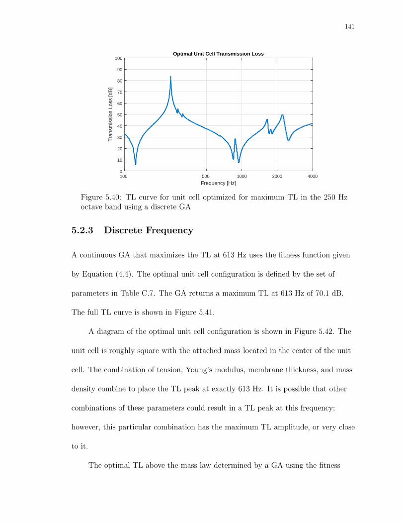
141

Frequency [Hz]100 500 1000 2000 4000

Tra

nsm

issi

on L

oss

[dB

]

0

10

20

30

40

50

60

70

80

90


Figure 5.40: TL curve for unit cell optimized for maximum TL in the 250 Hzoctave band using a discrete GA

5.2.3 Discrete Frequency

A continuous GA that maximizes the TL at 613 Hz uses the fitness function given

by Equation (4.4). The optimal unit cell configuration is defined by the set of

parameters in Table C.7. The GA returns a maximum TL at 613 Hz of 70.1 dB.

The full TL curve is shown in Figure 5.41.

A diagram of the optimal unit cell configuration is shown in Figure 5.42. The

unit cell is roughly square with the attached mass located in the center of the unit

cell. The combination of tension, Young’s modulus, membrane thickness, and mass

density combine to place the TL peak at exactly 613 Hz. It is possible that other

combinations of these parameters could result in a TL peak at this frequency;

however, this particular combination has the maximum TL amplitude, or very close

to it.

The optimal TL above the mass law determined by a GA using the fitness

142

Frequency [Hz]100 500 1000 2000 4000

Tra

nsm

issi

on L

oss

[dB

]

0

10

20

30

40

50

60

70

80

90


Figure 5.41: TL curve for unit cell optimized for maximum TL at 613 Hz usinga continuous GA

X-dimenson [mm]-15 -10 -5 0 5 10 15

Y-d

imen

sion

[mm

]

-15

-10

-5

0

5

10

15


Figure 5.42: Diagram showing unit cell size and mass location of unit cell opti-mized for maximum TL at 613 Hz using a continuous GA

function given by Equation (4.7) is 45.6 dB above the mass law at 613 Hz. The TL

is plotted in Figure 5.43 and the parameter values are given in Table C.8.

Comparing to Figure 5.41, a slight decrease in TL occurs due to the reduction of the

total unit cell weight.

143

Frequency [Hz]100 500 1000 2000 4000

Tra

nsm

issi

on L

oss

[dB

]

0

10

20

30

40

50

60

70

80

90



Figure 5.43: TL curve for unit cell optimized for maximum TL above the masslaw at 613 Hz using a continuous GA

Using a discrete GA to choose from a selection of materials to maximize TL at

613 Hz results in the TL plotted in Figure 5.44 and design variable values given in

Table C.9. The resulting TL at 613 Hz is 76.2 dB. The chosen materials for the

membrane and attached mass are polyester and lead, respectively. The width and

length of the attached mass are maximized. The size of the unit cell, tension on the

membrane, and thickness of the attached mass combine to place the TL peak at 613

Hz.

5.2.4 Multiple Discrete Frequencies

An optimal unit cell configuration to construct a membrane-type acoustic

metamaterial noise barrier to attenuate the sound source presented in Section 4.3.4

is designed using a continuous GA operating on the fitness function given by

Equation (4.5). The results are plotted in Figure 5.45 and given in Table C.10. The

144

Frequency [Hz]100 500 1000 2000 4000

Tra

nsm

issi

on L

oss

[dB

]

0

10

20

30

40

50

60

70

80

90


Figure 5.44: TL curve for unit cell optimized for maximum TL at 613 Hz usinga discrete GA

maximum fitness function value is 109.8 dB, which corresponds to the weighted sum

of TL at 361 Hz, 720 Hz, and 1319 Hz. Their weights are 1, 0.6, and 0.5,

respectively.

Frequency [Hz]100 500 1000 2000 4000

Tra

nsm

issi

on L

oss

[dB

]

0

10

20

30

40

50

60

70

80

90


Figure 5.45: TL curve for unit cell optimized for maximum TL for multipleweighted components using a continuous GA

The optimal unit cell size and shape is shown in Figure 5.46. The resulting

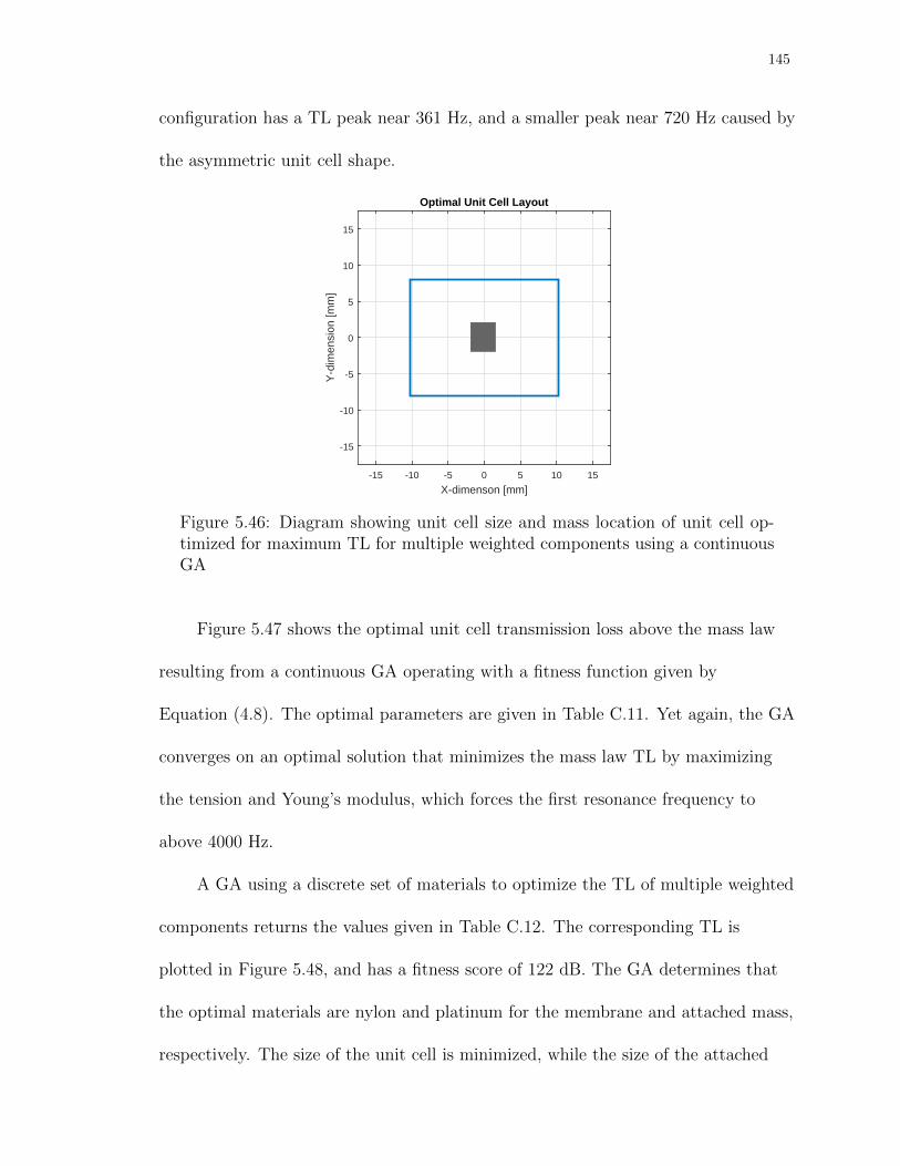
145

configuration has a TL peak near 361 Hz, and a smaller peak near 720 Hz caused by

the asymmetric unit cell shape.

X-dimenson [mm]-15 -10 -5 0 5 10 15

Y-d

imen

sion

[mm

]

-15

-10

-5

0

5

10

15


Figure 5.46: Diagram showing unit cell size and mass location of unit cell op-timized for maximum TL for multiple weighted components using a continuousGA

Figure 5.47 shows the optimal unit cell transmission loss above the mass law

resulting from a continuous GA operating with a fitness function given by

Equation (4.8). The optimal parameters are given in Table C.11. Yet again, the GA

converges on an optimal solution that minimizes the mass law TL by maximizing

the tension and Young’s modulus, which forces the first resonance frequency to

above 4000 Hz.

A GA using a discrete set of materials to optimize the TL of multiple weighted

components returns the values given in Table C.12. The corresponding TL is

plotted in Figure 5.48, and has a fitness score of 122 dB. The GA determines that

the optimal materials are nylon and platinum for the membrane and attached mass,

respectively. The size of the unit cell is minimized, while the size of the attached

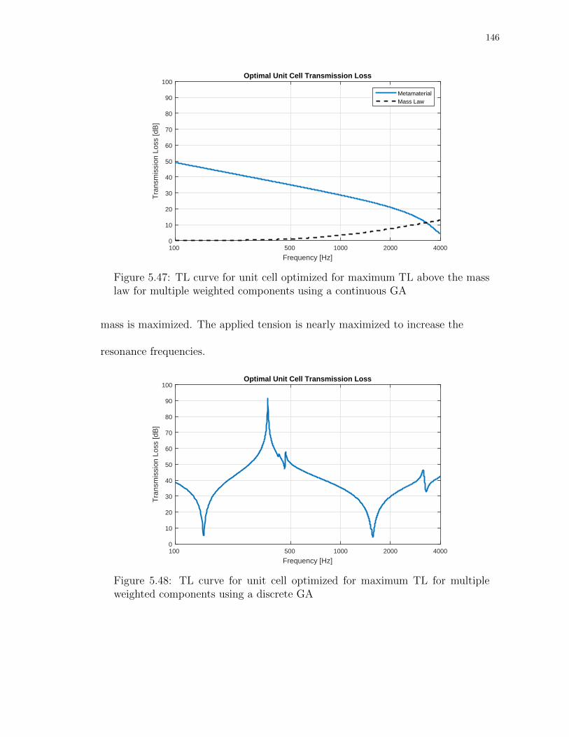
146

Frequency [Hz]100 500 1000 2000 4000

Tra

nsm

issi

on L

oss

[dB

]

0

10

20

30

40

50

60

70

80

90



Figure 5.47: TL curve for unit cell optimized for maximum TL above the masslaw for multiple weighted components using a continuous GA

mass is maximized. The applied tension is nearly maximized to increase the

resonance frequencies.

Frequency [Hz]100 500 1000 2000 4000

Tra

nsm

issi

on L

oss

[dB

]

0

10

20

30

40

50

60

70

80

90


Figure 5.48: TL curve for unit cell optimized for maximum TL for multipleweighted components using a discrete GA

147


The above sections illustrate the necessity and ease of applying an optimization

scheme using genetic algorithms to membrane-type acoustic metamaterials. In

Section 5.1 each design variable is manipulated independently to show the effect on

TL, and to provide context to the problem of designing membrane-type acoustic

metamaterials to achieve a noise reduction goal. The near-infinite number of

possible unit cell configurations makes it practically impossible to design a globally

optimal configuration.

GAs provide a tool for the noise control engineer to begin the design of

membrane-type acoustic metamaterial noise barriers. Section 5.2 highlights ways

that GAs can be used in the design process for a variety of noise reduction goals. By

running a GA that allows the design variables to take any value within a specified

range, inferences can be made based on the results. Critical design parameters can

be identified by noticing which values are maximized or minimized, and which sets

of values work co-dependently to achieve a maximum fitness function value. The

process can be repeated with a more specific design goal that is reflected in the

fitness function. Fitness functions can be altered based on previous results to

account for the new information gained, such as when the GA maximizes the overall

weight of the unit cell to increase TL. Finally, a discrete GA can be used to

determine which out of a set of available materials can be used together to create an

optimal unit cell configuration.

148

Chapter 6

Conclusion and Recommendations for

Future Work

6.1 Conclusion

To solve the problem of low frequency noise in environments with strict size and

weight limitations, noise control engineers propose membrane-type acoustic

metamaterials. Rapid design and optimization, however, cannot occur without

efficient and accurate models. This dissertation presents the formulation of

computationally efficient dynamic models of membrane-type acoustic metamaterials

using the impedance-mobility approach, the verification of their accuracy using a

finite element method, and the application of genetic algorithms to optimize their

structure.

The impedance-mobility approach is used to model membrane-type acoustic

metamaterial unit cells in a waveguide and in a baffle. By expanding the

149

displacement of unit cell as a summation of normal modes and considering the

coupling to the surrounding fluid, the vibratory response is determined. The models

are expanded to larger systems of layers of unit cells in a waveguide by coupling two

unit cells and a separating acoustic cavity. The response of arrays of unit cells in a

baffle is found two ways; by considering the coupled acoustic pressure due to

adjacent unit cells, and by neglecting the coupling entirely. Formulas for

transmission loss, reflection and absorption coefficients, effective mass density, panel

kinetic energy, and cavity potential energy are presented. The flexibility of these

models enable expansion to larger systems comprised of metamaterials, or

conventional materials. This method is also valid for higher frequencies when more

modes are included in the expansion of unit cell displacement and cavity pressure,

with the caveat that internal resonances in the attached mass can cause inaccuracy

with a large number of modes.

The accuracy of TL calculated using the impedance-mobility approach is

verified by comparison to FEM models. In general the models agree very well with

each other, and, by extension through previous work, to experimental results. The

assumptions of the impedance-mobility models are validated, and generalizations to

unit cells of different shapes are made. The results of the analysis in Chapters 3 and

5 indicate that the primary design variables responsible for the TL profile are the

applied tension on the membrane and the magnitude of the attached mass. For unit

cells of equal area, the shape of the unit cell does not significantly impact the TL. In

designing membrane-type acoustic metamaterial noise barriers, the shape of the unit

cell can be determined by external factors, such as ease of fabrication. For

150

regular-polygonal unit cell shapes with centrally-located attached masses, the

impedance-mobility model of a square unit cell with an equivalent area can be used

to accurately predict the TL response.

The process of design is greatly facilitated by optimization schemes capable of

sorting through the myriad possible configurations of unit cells. The GAs presented

in Chapter 4 are used in several ways to serve this purpose. First, the design criteria

are determined and a fitness function to quantify the degree of success is formulated.

Second, the GA is used to identify the key design variables by considering each one

as capable of taking any value in a predefined range. This enables the user to see

which variables are maximized or minimized, and which variables work in tandem to

determine the response of the structure. Third, the fitness function or design

variable ranges are adjusted according to the information gained from the output of

the first GA. Lastly, the GA is implemented such that it chooses from a finite set of

available materials that can be used in fabrication.

The fitness functions and material choices used in this dissertation are intended

as guidelines, and are by no means the only possible choices. The process described

above is a flexible framework that allows noise control engineers to incorporate their

experience into the process. While it is possible to design an adequate noise barrier

using a trial and error method with the GUI implementation of the

impedance-mobility model, a process involving GAs will find an optimal solution.

The work in this dissertation has lead to several novel contributions to the

field. An impedance mobility approach is used to model the transmission loss of a

vibrating structure in a waveguide, and in a baffle. Previous work has only

151

considered the transmission into a cavity from a flexible barrier, not through a

barrier or through a pair of barriers and cavity [Jin et al. 2009; Kim & Brennan

1999]. The response of a unit cell of a membrane-type acoustic metamaterial in a

baffle has not been previously studied. The impedance-mobility model is expanded

to consider multiple unit cells layered in series, and arrayed in a baffle. To date no

other analytical formulation of an array of unit cells has been presented. Genetic

algorithms are used to find the optimal unit cell configurations for various noise

control criteria.

6.2 Recommendations for Future Work

Future work should exploit the flexible formulation of the impedance-mobility

approach, which is ideal for expansion to larger and more complex

structural-acoustic systems. In addition to membrane-type acoustic metamaterials,

other noise control devices can be incorporated in layers. Micro-perforated panels

(MPPs) are an ideal candidate since they can be characterized in a manner that is

similar to the impedance-mobility approach [Bravo et al. 2012]. MPPs can also be

tuned to operate at a higher frequency range than that of membrane-type acoustic

metamaterials resulting in a broadband noise barrier. Other conventional materials

such as mass-loaded vinyl or fiberglass can be combined with membrane-type

acoustic metamaterials to create noise barriers that are effective over a wide

frequency range.

Genetic algorithms can also be used to optimize noise barriers that consist of

152

multiple conventional or metamaterial components. Continuous GAs can be used to

find optimal parameter values to optimize each substructure, and discrete GAs can

be used to pick the best combination of pre-fabricated components.

The impedance-mobility approach can be expanded to model the TL of double

layers of arrayed unit cells. The two layers could consist of multiple sets of unit cells

and cavities, or two arrays with a common cavity.

Another application of membrane-type acoustic metamaterials is absorption of

incident sound. The impedance-mobility models formulated in Chapter 2 are

primarily concerned with sound transmission through a structure, but can easily be

adapted to consider absorption. Ma et al. [2014] proposed a structure with a unit

cell consisting of a membrane carrying an attached mass suspended over a

rigid-walled cavity as shown in Figure 6.1. This structure is capable of perfect

absorption of an incident wave in a specific frequency band.

Pi

Pr

Lx

Lz

MA

Figure 6.1: Cross-section of a membrane-type acoustic metamaterial absorber

Further experimental verification of the models is also required. Small-scale

testing of unit cells in a plane-wave tube can ensure that optimal unit cell

configurations perform as intended. Large-scale measurement of membrane-type

acoustic metamaterial barriers is also needed.

153

Bibliography

ANSI (2004). ANSI S1.11: Specification for Octave, Half-Octave, and Third Octave

Band Filter Sets. Standard S1.11. American National Standards Institute.

ASHRAE (2011). “ASHRAE Handbook: HVAC Applications”. Chap. 48 Noise and

Vibration Control.

D. Bies & C. Hansen (2009). Engineering Noise Control: Theory and Practice.

Taylor & Francis.

T. Bravo, C. Maury, & C. Pinhede (2012). “Sound absorption and transmission

through flexible micro-perforated panels backed by an air layer and a thin plate”.

The Journal of the Acoustical Society of America 131.5, pp. 3853–3863.

C. T. Chan, J. Li, & K. H. Fung (2006). “On extending the concept of double

negativity to acoustic waves”. Journal of Zhejiang University Science A 7.1,

pp. 24–28.

J.-D. Chazot & J.-L. Guyader (2007). “Prediction of transmission loss of double

panels with a patch-mobility method”. The Journal of the Acoustical Society of

America 121.1, pp. 267–278.

154

H. Chen & C. Chan (2007). “Acoustic cloaking in three dimensions using acoustic

metamaterials”. Applied Physics Letters 91.18, p. 183518.

Y. Chen, G. Huang, X. Zhou, G. Hu, & C.-T. Sun (2014a). “Analytical coupled

vibroacoustic modeling of membrane-type acoustic metamaterials: Membrane

model”. The Journal of the Acoustical Society of America 136.3, pp. 969–979.

Y. Chen, G. Huang, X. Zhou, G. Hu, & C.-T. Sun (2014b). “Analytical coupled

vibroacoustic modeling of membrane-type acoustic metamaterials: Plate model”.


Y. Cheng, F. Yang, J. Y. Xu, & X. J. Liu (2008). “A multilayer structured acoustic

cloak with homogeneous isotropic materials”. Applied Physics Letters 92.15,

p. 151913.

A. Climente, D. Torrent, & J. Sanchez-Dehesa (2010). “Sound focusing by gradient

index sonic lenses”. Applied Physics Letters 97.10, p. 104103.

COMSOL Multiphysics (2012). “COMSOL Multiphysics User Guide (Version 4.3 a)”.

R. V. Craster & S. Guenneau (2012). Acoustic Metamaterials: Negative Refraction,

Imaging, Lensing and Cloaking. Vol. 166. Springer.

S. Das (2009). “Metamaterials arrive in cellphones”. IEEE Spectrum.

K. A. De Jong & W. M. Spears (1992). “A formal analysis of the role of multi-point

crossover in genetic algorithms”. Annals of mathematics and Artificial

intelligence 5.1, pp. 1–26.

K. Deb (1999). “An introduction to genetic algorithms”. Sadhana 24.4-5,

pp. 293–315.

155

C.-L. Ding & X.-P. Zhao (2011). “Multi-band and broadband acoustic metamaterial

with resonant structures”. Journal of Physics D: Applied Physics 44.21,

p. 215402.

M. Dorigo, V. Maniezzo, & A. Colorni (1996). “Ant system: optimization by a

colony of cooperating agents”. Systems, Man, and Cybernetics, Part B:

Cybernetics, IEEE Transactions on 26.1, pp. 29–41.

E. Dowell, G. Gorman III, & D. Smith (1977). “Acoustoelasticity: general theory,

acoustic natural modes and forced response to sinusoidal excitation, including

comparisons with experiment”. Journal of Sound and Vibration 52.4,

pp. 519–542.

E. Elbeltagi, T. Hegazy, & D. Grierson (2005). “Comparison among five

evolutionary-based optimization algorithms”. Advanced engineering informatics

19.1, pp. 43–53.

S. J. Elliott (1999). “Down with noise”. IEEE Spectrum 36.6, pp. 54–61.

S. J. Elliott & P. A. Nelson (1993). “Active noise control”. Signal Processing

Magazine, IEEE 10.4, pp. 12–35.

F. A. Everest (2001). The Master Handbook of Acoustics. Vol. 4. McGraw-Hill New

York.

F. J. Fahy & P. Gardonio (2007). Sound and Structural Vibration: Radiation,

Transmission and Response. Academic Press.

F. Fahy & J. Walker (2004). Advanced Applications in Acoustics, Noise and

Vibration. CRC Press.

156

N. Fang, H. Lee, C. Sun, & X. Zhang (2005). “Sub–diffraction-limited optical

imaging with a silver superlens”. Science 308.5721, pp. 534–537.

N. Fang, D. Xi, J. Xu, M. Ambati, W. Srituravanich, C. Sun, & X. Zhang (2006).

“Ultrasonic metamaterials with negative modulus”. Nature Materials 5.6,

pp. 452–456.

M. J. Freire, L. Jelinek, R. Marques, & M. Lapine (2010). “On the applications of

µr=-1 metamaterial lenses for magnetic resonance imaging”. Journal of Magnetic

Resonance 203.1, pp. 81–90.

P. Gardonio & M. Brennan (2002). “On the origins and development of mobility and

impedance methods in structural dynamics”. Journal of Sound and Vibration

249.3, pp. 557–573.

D. E. Goldberg & K. Deb (1991). “A comparative analysis of selection schemes used

in genetic algorithms”. Foundations of Genetic Algorithms.

S. Guenneau, A. Movchan, G. Petursson, & S. A. Ramakrishna (2007). “Acoustic

metamaterials for sound focusing and confinement”. New Journal of Physics

9.11, p. 399.

R. L. Haupt (1995). “An introduction to genetic algorithms for electromagnetics”.

Antennas and Propagation Magazine, IEEE 37.2, pp. 7–15.

K. M. Ho, C. K. Cheng, Z. Yang, X. Zhang, & P. Sheng (2003). “Broadband locally

resonant sonic shields”. Applied Physics Letters 83.26, pp. 5566–5568.

J. H. Holland (1975). Adaptation in Natural and Artificial Systems: An Introductory

Analysis with Applications to Biology, Control, and Artificial Intelligence. U

Michigan Press.

157

S. James (2005). Defining the Cockpit Noise Hazard, Aircrew Hearing Damage Risk

and the Benefits Active Noise Reduction Headsets can Provide. Tech. rep. DTIC

Document.

Z. H. Jiang, J. A. Bossard, X. Wang, & D. H. Werner (2011). “Synthesizing

metamaterials with angularly independent effective medium properties based on

an anisotropic parameter retrieval technique coupled with a genetic algorithm”.

Journal of Applied Physics 109.1, p. 013515.

G. Jin, Z. Liu, & T. Yang (2009). “Active control of sound transmission into an

acoustic cavity surrounded by more than one flexible plate”. Noise Control

Engineering Journal 57.3, pp. 210–220.

J. Kennedy (1997). “The particle swarm: social adaptation of knowledge”.

Evolutionary Computation, 1997., IEEE International Conference on. IEEE,

pp. 303–308.

S. M. Kim (1999). “Active control of sound in structural-aocustic systems”. PhD

Thesis. University of Southampton.

S. M. Kim & M. J. Brennan (1999). “A compact matrix formulation using the

impedance and mobility approach for the analysis of structural-acoustic

systems”. Journal of Sound and Vibration 223.1, pp. 97–113.

L. E. Kinsler, A. R. Frey, A. B. Coppens, & J. V. Sanders (2000). Fundamentals of

Acoustics. 4th ed. Wiley.

O. Kopmaz & S. Telli (2002). “Free vibrations of a rectangular plate carrying a

distributed mass”. Journal of Sound and Vibration 251.1, pp. 39–57.

158

F. Langfeldt, W. Gleine, & O. von Estorff (2015). “Analytical model for

low-frequency transmission loss calculation of membranes loaded with arbitrarily

shaped masses”. Journal of Sound and Vibration 349, pp. 315–329.

S. Lau & S. Tang (2001). “Sound fields in a rectangular enclosure under active

sound transmission control”. The Journal of the Acoustical Society of America

110.2, pp. 925–938.

S. Lau & S. Tang (2006). “Sound attenuation pattern in a rectangular enclosure

under potential-energy based active sound transmission control”. INTER-NOISE

and NOISE-CON Congress and Conference Proceedings. Vol. 2006. 5. Institute

of Noise Control Engineering, pp. 2582–2591.

J. D. Leatherwood (1987). Annoyance Response to Simulated Advanced Turboprop

Aircraft Interior Noise Containing Tonal Beats. Tech. rep. 2689. NASA.

A. W. Leissa (1969). Vibration of Plates. Tech. rep. DTIC Document.

H. Leventhall (2004). “Low frequency noise and annoyance”. Noise & Health 6.23,

pp. 59–72.

D. Li, L. Zigoneanu, B.-I. Popa, & S. A. Cummer (2012). “Design of an acoustic

metamaterial lens using genetic algorithms”. The Journal of the Acoustical

Society of America 132.4, pp. 2823–2833.

J. Li & C. T. Chan (2004). “Double-negative acoustic metamaterial”. Physical

Review E 70.5, p. 055602.

J. Li, Z. Liu, & C. Qiu (2006). “Negative refraction imaging of acoustic waves by a

two-dimensional three-component phononic crystal”. Physical Review B 73.5,

p. 054302.

159

P. Li, S. Yao, X. Zhou, G. Huang, & G. Hu (2014). “Effective medium theory of

thin-plate acoustic metamaterials”. The Journal of the Acoustical Society of

America 135.4, pp. 1844–1852.

X.-F. Li, X. Ni, L. Feng, M.-H. Lu, C. He, & Y.-F. Chen (2011). “Tunable

unidirectional sound propagation through a sonic-crystal-based acoustic diode”.

Physical Review Letters 106.8, p. 084301.

Z. Liu, X. Zhang, Y. Mao, Y. Y. Zhu, Z. Yang, C. T. Chan, & P. Sheng (2000).

“Locally resonant sonic materials”. Science 289.5485, pp. 1734–1736.

M. Long (2006). Architectural Acoustics. Academic Press.

K. Lu, J. H. Wu, D. Guan, N. Gao, & L. Jing (2016). “A lightweight low-frequency

sound insulation membrane-type acoustic metamaterial”. AIP Advances 6.2,

p. 025116.

G. Ma, M. Yang, S. Xiao, Z. Yang, & P. Sheng (2014). “Acoustic metasurface with

hybrid resonances”. Nature Materials 13.9, pp. 873–878.

MathWorks (2016). MathWorks MATLAB Runtime. url:

http://www.mathworks.com/products/compiler/mcr/ (visited on

03/18/2016).

L. Maxit, C. Yang, L. Cheng, & J.-L. Guyader (2012). “Modeling of

micro-perforated panels in a complex vibro-acoustic environment using patch

transfer function approach”. The Journal of the Acoustical Society of America

131.3, pp. 2118–2130.

http://www.mathworks.com/products/compiler/mcr/

160

H. Meng, J. Wen, H. Zhao, & X. Wen (2012). “Optimization of locally resonant

acoustic metamaterials on underwater sound absorption characteristics”. Journal

of Sound and Vibration 331.20, pp. 4406–4416.

P. Merz & B. Freisleben (1997). “A genetic local search approach to the quadratic

assignment problem”. Proceedings of the 7th international conference on genetic

algorithms, pp. 1–1.

M. Mitchell (1998). An Introduction To Genetic Algorithms. MIT Press.

H. Møller & C. S. Pedersen (2011). “Low-frequency noise from large wind turbines”.


S. More & P. Davies (2010). “Human responses to the tonalness of aircraft noise”.

Noise Control Engineering Journal 58.4, pp. 420–440.

C. J. Naify, C. M. Chang, G. McKnight, & S. R. Nutt (2010). “Transmission loss

and dynamic response of membrane-type locally resonant acoustic

metamaterials”. Journal of Applied Physics 108.11, p. 114905.

C. J. Naify, C. M. Chang, G. McKnight, & S. R. Nutt (2011a). “Transmission loss of

membrane-type acoustic metamaterials with coaxial ring masses”. Journal of

Applied Physics 110.12, p. 124903.

C. J. Naify, C. M. Chang, G. McKnight, & S. R. Nutt (2012). “Scaling of

membrane-type locally resonant acoustic metamaterial arrays”. Journal of the

Acoustical Society of America 132.4, pp. 2784–2792.

C. J. Naify, C. M. Chang, G. McKnight, F. Scheulen, & S. Nutt (2011b).

“Membrane-type metamaterials: Transmission loss of multi-celled arrays”.

Journal of Applied Physics 109.10, p. 104902.

161

C. J. Naify, C. Huang, M. Sneddon, & S. Nutt (2011c). “Transmission loss of

honeycomb sandwich structures with attached gas layers”. Applied Acoustics

72.2, pp. 71–77.

M. Ouisse, L. Maxit, C. Cacciolati, & J.-L. Guyader (2005). “Patch transfer

functions as a tool to couple linear acoustic problems”. Journal of vibration and

Acoustics 127.5, pp. 458–466.

J. B. Pendry, A. J. Holden, W. J. Stewart, & I. Youngs (1996). “Extremely low

frequency plasmons in metallic mesostructures”. Physical Review Letters 76.25,

p. 4773.

J. Pendry & J. Li (2008). “An acoustic metafluid: realizing a broadband acoustic

cloak”. New Journal of Physics 10.11, p. 115032.

J. B. Pendry (2000). “Negative refraction makes a perfect lens”. Physical Review

Letters 85.18, p. 3966.

E. E. Ryherd & L. M. Wang (2008). “Implications of human performance and

perception under tonal noise conditions on indoor noise criteria”. The Journal of

the Acoustical Society of America 124.1, pp. 218–226.

E. A. G. Shaw & G. J. Thiessen (1962). “Acoustics of circumaural earphones”. The

Journal of the Acoustical Society of America 34.9A.

P. Sheng, J. Mei, Z. Liu, & W. Wen (2007). “Dynamic mass density and acoustic

metamaterials”. Physica B: Condensed Matter 394.2, pp. 256–261.

L. W. T. Silva, V. F. Barros, & S. G. Silva (2014). “Genetic algorithm with

maximum-minimum crossover (GA-MMC) applied in optimization of radiation

162

pattern control of phased-array radars for rocket tracking systems”. Sensors

14.8, pp. 15113–15141.

D. R. Smith, J. B. Pendry, & M. C. K. Wiltshire (2004). “Metamaterials and

negative refractive index”. Science 305.5685, pp. 788–792.

S. D. Snyder & N. Tanaka (1995). “Calculating total acoustic power output using

modal radiation efficiencies”. The Journal of the Acoustical Society of America

97.3, pp. 1702–1709.

H. Tian, X. Wang, & Y.-h. Zhou (2014). “Theoretical model and analytical

approach for a circular membrane–ring structure of locally resonant acoustic

metamaterial”. Applied Physics A 114.3, pp. 985–990.

N. Totaro & J.-L. Guyader (2012). “Efficient positioning of absorbing material in

complex systems by using the Patch Transfer Function method”. Journal of

Sound and Vibration 331.13, pp. 3130–3143.

V. G. Veselago (1968). “The electrodynamics of substances with simultaneously

negative values of ε and µ”. Physics-Uspekhi 10.4, pp. 509–514.

C. E. Wallace (1972). “Radiation resistance of a rectangular panel”. The Journal of

the Acoustical Society of America 51.3B, pp. 946–952.

R. Wang, B. Yuan, G. Wang, & F. Yi (2007). “Efficient design of directive patch

antennas in mobile communications using metamaterials”. International Journal

of Infrared and Millimeter Waves 28.8, pp. 639–649.

E. C. Wester, X. Bremaud, & B. Smith (2009). “Meta-material sound insulation”.

Building Acoustics 16.1, pp. 21–30.

163

J. F. Wilby (1996). “Aircraft interior noise”. Journal of Sound and Vibration 190.3,

pp. 545–564.

Z. Yang, H. M. Dai, N. H. Chan, G. C. Ma, & P. Sheng (2010). “Acoustic

metamaterial panels for sound attenuation in the 50–1000 Hz regime”. Applied

Physics Letters 96.4, p. 041906.

Z. Yang, J. Mei, M. Yang, N. Chan, & P. Sheng (2008). “Membrane-type acoustic

metamaterial with negative dynamic mass”. Physical Review Letters 101.20,

p. 204301.

Y. Zhang, J. Wen, Y. Xiao, X. Wen, & J. Wang (2012). “Theoretical investigation of

the sound attenuation of membrane-type acoustic metamaterials”. Physics

Letters A 376.17, pp. 1489–1494.

Y. Zhang, J. Wen, H. Zhao, D. Yu, L. Cai, & X. Wen (2013). “Sound insulation

property of membrane-type acoustic metamaterials carrying different masses at

adjacent cells”. Journal of Applied Physics 114.6, p. 063515.

H.-G. Zhao, Y.-Z. Liu, J.-H. Wen, D.-L. Yu, G. Wang, & X.-S. Wen (2006). “Sound

absorption of locally resonant sonic materials”. Chinese Physics Letters 23.8,

p. 2132.

H.-G. Zhao, Y.-Z. Liu, J.-H. Wen, D.-L. Yu, & X.-S. Wen (2007). “Tri-component

phononic crystals for underwater anechoic coatings”. Physics Letters A 367.3,

pp. 224–232.

O. C. Zienkiewicz, R. L. Taylor, O. C. Zienkiewicz, & R. L. Taylor (1977). The

Finite Element Method. Vol. 3. McGraw-Hill London.

164

Appendix A

Modes and Modal Radiation Efficiencies

The impedance-mobility formulation described in Chapter 2 uses a mode

superposition method to describe the vibratory motion of the unit cell. To assist in

understanding this method, this appendix describes the modes of vibration and

natural frequencies of a simply supported membrane with and without bending

stiffness. The modes and natural frequencies of a rigid-walled cavity are explained to

elucidate the impedance-mobility formulation for a double layer of membrane-type

acoustic metamaterial unit cells. The modal radiation efficiencies used to calculate

the sound power radiated by a unit cell in a rigid baffle are also explained here.

165

A.1 Vibration Modes and Natural Frequencies of

a Simply Supported Membrane

A.1.1 Modeshape Function

The equation of motion for a membrane without external forces is

ρs∂2w

∂t2− T∇2w = 0, (A.1)

where w is the out-of-plane deflection, ρs is the surface density, and T is the applied

tension. By applying simply supported boundary conditions for a membrane of

dimensions Lx × Ly

w(0, y) = w(Lx, y) = w(x, 0) = w(x, Ly) = 0,

and using separation of variables, it can be shown that the mode functions are

sinusoids given by

φm(x, y) = 2 sin

(m1πx

Lx

)sin

(m2πy

Ly

), (A.2)

where the structural modes are m = (m1,m2).

166

A.1.2 Natural Frequencies

The wave numbers are restricted to values of kx = m1π/Lx and ky = m2π/Ly, which

restricts the natural frequencies to

ωm =

√T

ρs

√(m1π

Lx

)2

+

(m2π

Ly

)2

, (A.3)

where m = 1, 2, ...M

A.1.3 Membrane Stiffness

Incorporating membrane bending stiffness into Equation (A.1) gives

ρs∂2w

∂t2+D∇4w − T∇2w = 0, (A.4)

with corresponding natural frequencies

ωm =

√T

ρs

√(m1π

Lx

)2

+

(m2π

Ly

)2

+

√D

ρs

[(m1π

Lx

)2

+

(m2π

Ly

)2], (A.5)

where D is the membrane flexural rigidity given by

D =Eh3

12(1− ν2). (A.6)

E, h, and ν are the membrane’s Young’s modulus, thickness, and Poisson’s ratio,

respectively [Leissa 1969]. The modeshapes of a membrane with bending stiffness

are identical to those given by Equation (A.2).

167

A.2 Acoustic Modes and Natural Frequencies of

a Rigid-walled Cavity

For a rectangular cavity of dimensions Lx × Ly × Lz with perfectly rigid walls, the

spatial component of the sound pressure satisfies the Helmholtz equation

∇2ψ + k2ψ = 0. (A.7)

Using separation of variables and applying the rigid walled boundary condition

where the normal component of the particle velocity is zero on the boundaries, it

can be shown that the acoustic modeshapes follow the form

ψn(x, y, z) =√e1e2e3 cos

(n1πx

Lx

)cos

(n2πy

Ly

)cos

(n3πz

Lz

), (A.8)

for acoustic mode n = (n1, n2, n3) where ei = 1 for ni = 0 and ei = 2 if ni > 0 for

i = 1, 2, or 3. The natural frequencies are then given by

ωn = c

√(n1π

Lx

)2

+

(n2π

Ly

)2

+

(n3π

Lz

)2

. (A.9)

A.3 Series Truncation

Expressing membrane vibration amplitudes and cavity pressures in a matrix-vector

form using mode superposition requires that summations be truncated at a finite

number of modes, M and N for structural and acoustic modes, respectively.

168

Figure A.1 shows the normal modes within an arbitrary frequency range, ω, for a

membrane of dimensions Lx × Ly. The modes included in the summation are those

that fall within the specified frequency range, colored in red. For the normal modes

of an acoustic cavity, one can imagine A.1 in three dimensions with the included

modes being the combination of modal coordinates that fall within one octant of an

enclosing sphere.

kx

ky

ω/c

π/Lx

π/Ly

1 2 3 4 5 6 7 8

1

2

3

4

5

6

7

8

Mode (5,3)

Figure A.1: Normal modes of an Lx × Ly membrane in k-space

Conventionally, the natural frequencies of the included modes must span a

range that is two octaves higher than the highest frequency of interest [Bies &

Hansen 2009]. However, in practice for a membrane carrying an attached mass the

number of modes must be kept low to avoid internal resonances [Tian et al. 2014;

Zhang et al. 2012]. In the research presented in this dissertation, the number of

modes was held constant at M = N = 9, corresponding to a little under one octave

above the highest frequency of interest. The modes and their corresponding

169

resonance frequencies for the baseline double panel configuration are shown in

Figure A.2. Note that the cavity resonance frequencies are well outside of the

frequency range of interest from 100 Hz to 4000 Hz with the exception of the

fundamental mode.

Mode Number1 2 3 4 5 6 7 8 9

Res

onan

ce F

requ

ency

[kH

z]

0

5

10

15

20

25Included Modes

CavityUnit Cell AUnit Cell B

Figure A.2: Resonance frequencies of acoustic and structural modes included infinite summations

A.4 Modal Radiation Efficiences

The modal radiation efficiencies needed to compute the power transfer matrix

(Equation (2.19)) are given by Equations (33), (38), and (43) in Snyder & Tanaka

[1995], reproduced below with the notation used in this dissertation. The equations

are separated into even and odd modes giving four separate equations. For a mode

170

α = (m1,m2)

σα =32k2LxLym2

1m22π

5

{1− k2LxLy

12

[(1− 8

m21π

2

)LxLy

+

(1− 8

m22π

2

)LyLx

]}, (A.10)

for odd-odd modes;

σα =8k4L3

xLy3m2

1m22π

5

{1− k2LxLy

20

[(1− 24

m21π

2

)LxLy

+

(1− 8

m22π

2

)LyLx

]}, (A.11)

for even-odd modes;

σα =8k4LxL

3y

3m21m

22π

5

{1− k2LxLy

20

[(1− 8

m21π

2

)LxLy

+

(1− 24

m22π

2

)LyLx

]}, (A.12)

for odd-even modes; and

σα =2k6L3

xL3y

15m21m

22π

5

{1− k2LxLy

14

[(1− 24

m21π

2

)LxLy

+

(1− 24

m22π

2

)LyLx

]}, (A.13)

for odd-odd modes.

Figure A.3 shows the radiation efficiencies as a function of frequency.

171

Frequency [Hz]100 500 1000 2000 3000 4000

Rad

iatio

n E

ffici

ency

, σα

10-14

10-12

10-10

10-8

10-6

10-4

10-2

100Radiation Efficiencies

(1,1)(1,2) (2,1)(2,2)(1,3) (3,1)(2,3) (3,2)(3,3)

Figure A.3: Radiation efficiencies of included modes vs frequency

172

Appendix B

Tables

Table B.1: Baseline configuration parameter values

Parameter Symbol Value UnitsUnit cell width Lx 21 mmUnit cell height Ly 21 mmMembrane thickness tmem 0.0762 mmMembrane density ρmem 1200 kg/m3

Membrane tension T 5 MPaMembrane elastic modulus E 2.4 GPaMembrane Poisson’s ratio ν 0.35 -Mass density ρmass 19000 kg/m3

Mass elastic modulus Emass 170 GPaMass Poisson’s ratio νmass 0.3 -Mass thickness tmass 4.5 mmMass width lx 3 mmMass height ly 3 mmMass x location x0 9 mmMass y location y0 9 mm

173

Table B.2: Alternate configuration parameter values

Parameter Symbol Value UnitsUnit cell width Lx 21 mmUnit cell height Ly 21 mmMembrane thickness tmem 0.0762 mmMembrane density ρmem 1000 kg/m3

Membrane tension T 6 MPaMembrane elastic modulus E 2.4 GPaMembrane Poisson’s ratio ν 0.35 -Mass density ρmass 7000 kg/m3

Mass elastic modulus Emass 390 GPaMass Poisson’s ratio νmass 0.31 -Mass thickness tmass 6 mmMass width lx 3 mmMass height ly 3 mmMass x location x0 6 mmMass y location y0 9 mm

Table B.3: Design variable ranges

Parameter Symbol Units Minimum MaximumUnit cell width Lx mm 15 35Unit cell height Ly mm 15 35Membrane thickness tmem mm 0.0125 0.1506Membrane density ρmem kg/m3 900 2500Membrane tension T N/m 50 500Membrane elastic modulus E GPa 0.0008 5Membrane Poisson’s ratio ν - 0.3 0.5Mass density ρmass kg/m3 1000 20000Mass thickness tmass mm 1.5 6Mass width ratio lx,r - 0.01 0.25Mass height ratio ly,r - 0.01 0.25Mass x location ratio x0,r - 0.0625 0.5Mass y location ratio y0,r - 0.0625 0.5

174

Table B.4: Selected membrane material properties

Number Material Density Young’s Modulus Poisson’s Ratio[kg/m3] [GPa] [-]

0 Polypropylene 900 1.3 0.451 Natural Rubber 980 0.0008 0.482 Neoprene 1100 0.01 0.493 Nylon 1200 2.4 0.354 Polyester 1310 2.3 0.405 PVC 1400 2.8 0.406 PVDF 1760 1.5 0.357 PTFE 2200 0.5 0.46

Table B.5: Selected mass material properties

Number Material Density Young’s Modulus Poisson’s Ratio[kg/m3] [GPa] [-]

0 Magnesium 1740 44.7 0.291 Aluminum 2700 70 0.352 Titanium 4500 116 0.323 Neodymium 7000 390 0.314 Brass 8500 95 0.355 Lead 11,400 13.8 0.446 Tungsten 19,300 360 0.347 Platinum 21,400 168 0.27

Table B.6: Available mass sizes

Number lx [mm] ly [mm] tmass [mm]0 3 3 1.51 3 6 1.52 6 3 1.53 6 6 1.54 3 3 35 3 6 36 6 3 37 6 6 38 3 3 4.59 3 6 4.510 6 3 4.511 6 6 4.512 3 3 613 3 6 614 6 3 615 6 6 6

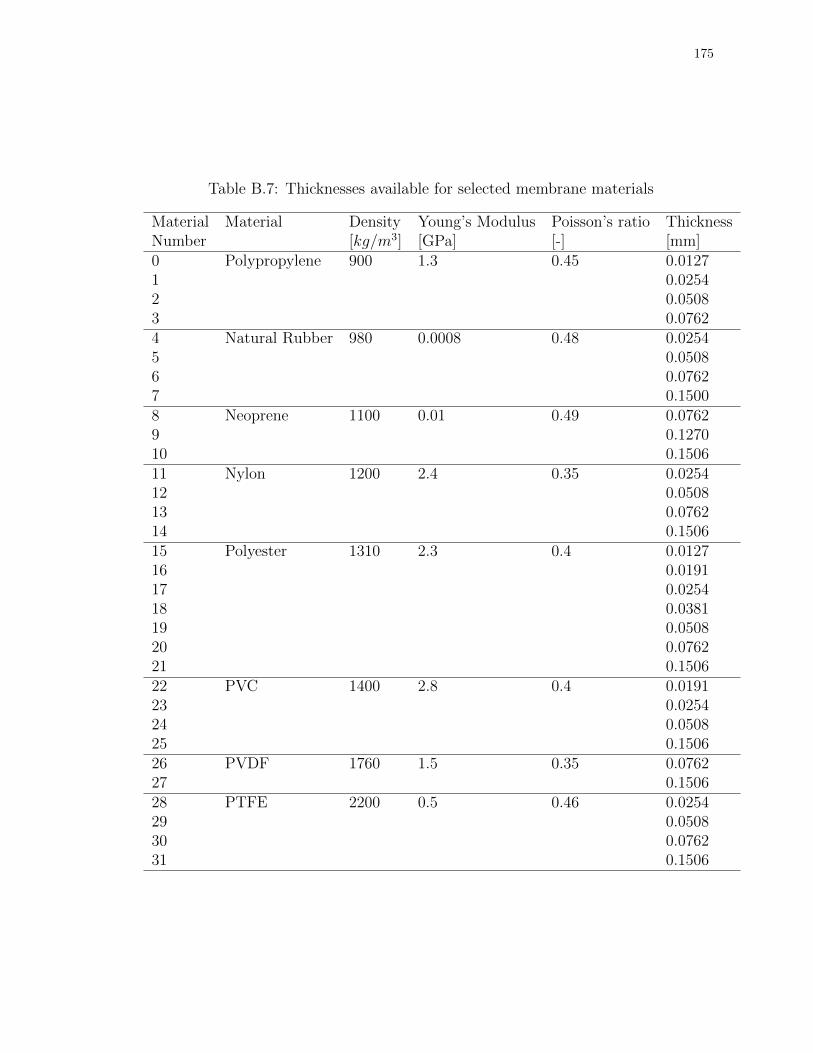
175

Table B.7: Thicknesses available for selected membrane materials

Material Material Density Young’s Modulus Poisson’s ratio ThicknessNumber [kg/m3] [GPa] [-] [mm]0 Polypropylene 900 1.3 0.45 0.01271 0.02542 0.05083 0.07624 Natural Rubber 980 0.0008 0.48 0.02545 0.05086 0.07627 0.15008 Neoprene 1100 0.01 0.49 0.07629 0.127010 0.150611 Nylon 1200 2.4 0.35 0.025412 0.050813 0.076214 0.150615 Polyester 1310 2.3 0.4 0.012716 0.019117 0.025418 0.038119 0.050820 0.076221 0.150622 PVC 1400 2.8 0.4 0.019123 0.025424 0.050825 0.150626 PVDF 1760 1.5 0.35 0.076227 0.150628 PTFE 2200 0.5 0.46 0.025429 0.050830 0.076231 0.1506

176

Table B.8: Finite element model details

Unit Cell Shape Air Domain Model Total Number Degrees Run Timeof Elements of Freedom (df = 10 Hz)

Square Waveguide Solid 69,178 211,922 17 hr 5 minSquare Baffle Shell 68,939 128,490 3 hr 46 min

2x1 Array Squares Baffle Shell 100,331 203,049 7 hr 21 min2x2 Array Squares Baffle Shell 159,240 344,513 13 hr 42 min

Double Square Waveguide Shell 81,558 166,407 4 hr 57 minSquare Simple Mass Waveguide Solid 68,106 207,590 15 hr 44 min

Square Waveguide Shell 49,506 96,093 2 hr 28 minCircle Waveguide Shell 59,776 122,373 3 hr 49 min

Circle Axi-symmetric Waveguide Solid 1051 3844 1 min 39 secHexagon Waveguide Shell 20,350 70,696 2 hr 7 minTriangle Waveguide Shell 27,195 62,628 1 hr 37 min

177

Appendix C

Genetic Algorithm Optimal

Results Tables

Table C.1: Optimal parameter values for maximum broadband TL using a con-tinuous GA

Parameter Symbol Value UnitsUnit cell width Lx 15.16 mmUnit cell height Ly 15.00 mmMembrane thickness tmem 0.1495 mmMembrane density ρmem 1127 kg/m3

Membrane tension T 393.7 N/mMembrane elastic modulus E 4.84 GPaMembrane Poisson’s ratio ν 0.45 -Mass density ρmass 18055 kg/m3

Mass thickness tmass 3.66 mmMass width lx 3.73 mmMass height ly 3.60 mmMass x location x0 5.18 mmMass y location y0 6.41 mm

178

Table C.2: Optimal parameter values for maximum broadband TL above themass law using a continuous GA




Table C.3: Optimal parameter values for maximum broadband TL using a dis-crete GA




179

Table C.4: Optimal parameter values for maximum TL in the 250 Hz octaveband using a continuous GA




Table C.5: Optimal parameter values for maximum TL above the mass law inthe 250 Hz octave band using a continuous GA




180

Table C.6: Optimal parameter values for maximum TL in the 250 Hz octaveband using a discrete GA




Table C.7: Optimal parameter values for maximum TL at 613 Hz using a con-tinuous GA




181

Table C.8: Optimal parameter values for maximum TL above the mass law at613 Hz using a continuous GA




Table C.9: Optimal parameter values for maximum TL at 613 Hz using a dis-crete GA




182

Table C.10: Optimal parameter values for maximum TL for multiple weightedcomponents using a continuous GA




Table C.11: Optimal parameter values for maximum TL above the mass law formultiple weighted components using a continuous GA




183

Table C.12: Optimal parameter values for maximum TL for multiple weightedcomponents using a discrete GA




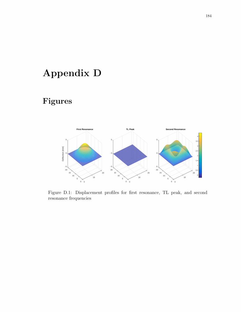
184

Appendix D

Figures

20

10

First Resonance

00

5

10

15

20

-5

0

5

Def

lect

ion

[mm

]

20

10

TL Peak

00

5

10

15

20

-5

0

5

20

10

Second Resonance

00

5

10

15

20

-5

0

5

0

0.5

1

1.5

2

2.5

3

3.5

4

Figure D.1: Displacement profiles for first resonance, TL peak, and secondresonance frequencies

185

Center Frequency [Hz]125 250 500 1000 2000 4000

Tra

nsm

issi

on L

oss

[dB

]

0

10

20

30

40

50

60

70

80

90

100Octave Band Transmission Loss

Figure D.2: TL of unit cell optimized for maximum TL in the 250 Hz octaveband using a continuous GA


Tra

nsm

issi

on L

oss

[dB

]

0

10

20

30

40

50

60

70

80

90



Figure D.3: TL of unit cell optimized for maximum TL above the mass law inthe 250 Hz octave band

186


Tra

nsm

issi

on L

oss

[dB

]

0

10

20

30

40

50

60

70

80

90


Figure D.4: TL of unit cell optimized for maximum TL in the 250 Hz octaveband using a discrete GA

187

Appendix E

Application of Boundary Conditions

For the simply supported case, in which the displacement of the membrane at

the boundaries is fixed at zero and the slope is unconstrained, the integrals derived

in Chapter 2 can easily be solved in a closed form. The closed-form solutions are

particularly amenable to hard-coding which greatly increases computational

efficiency. For that reason, the closed-form solutions to the integrals that form the

structural mobility matrix of the unit cell of a membrane-type acoustic

metamaterial are presented here.

For a simply supported membrane the area-normalized mode function is

written

φm(x, y) = 2 sin

(m1πx

Lx

)sin

(m2πy

Ly

). (E.1)

The terms defined in Chapter 2, Equations 2.6 - 2.10 and 2.26, can be solved

explicitly as follows

Mm = ρsLxLy, (E.2)

188

Qmn =−LxLyρmass

π2(m21 − n2

1)(m22 − n2

2)

{[(m1 + n1) sin

(π(m1 − n1)x0

Lx

)

−(m1 − n1) sin

(π(m1 + n1)x0

Lx

)− (m1 + n1) sin

(π(m1 − n1)(x0 + lx)

Lx

)

+(m1 − n1) sin

(π(m1 + n1)(x0 + lx)

Lx

) ][(m2 + n2) sin

(π(m2 − n2)y0

Ly

)

−(m2 − n2) sin

(π(m2 + n2)y0

Ly

)− (m2 + n2) sin

(π(m2 − n2)(y0 + ly)

Ly

)

+(m2 − n2) sin

(π(m2 + n2)(y0 + ly)

Ly

)]},

(E.3)

for m 6= n;

Qmm = ρmass

(lx −

Lx2m1π

(sin

(2πm1(x0 + lx)

Lx

)− sin

(2πm1x0

Lx

)))

(ly −

Ly2m2π

(sin

(2πm2(y0 + ly)

Ly

)− sin

(2πm2y0

Ly

))),

(E.4)

for m = n;

Km =Tπ2

LxLy

(m2

1L2x +m2

2L2y

), (E.5)

where m1 and m2 are modal indices of the mth structural mode,

Hm =2LxLym1m2π2

((−1)m1 − 1) ((−1)m2 − 1) , (E.6)

Dm = 2ρ0c0LxLy, (E.7)

189

and

Em =Dπ4

L3xL

3y

(m2

1L2y +m2

2L2x

)2. (E.8)

The coupling coefficient for a double layer structure given by Equation (2.63)

can be evaluated explicitly for structural mode m = (m1,m2) and acoustic cavity

mode n = (n1, n2, n3) as

CAm,n =

2√e1e2e3LxLym1m2 (1− (−1)m1+n1) (1− (−1)m2+n2)

π2 (m21 − n2

1) (m22 − n2

2)(E.9)

for unit cell A located at zi = 0, and

CBm,n =

2√e1e2e3LxLym1m2(−1)n3 (1− (−1)m1+n1) (1− (−1)m2+n2)

π2 (m21 − n2

1) (m22 − n2

2)(E.10)

for unit cell B located at zi = Lz. The term√e1e2e3 in the above equations is the

acoustic modeshape normalization factor where ei = 1 for ni = 0 and ei = 2 if

ni > 0. If m1 = n1 and/or m2 = n2, the value of the coupling coefficient is zero.

The generalized modal force due to an incident plane wave from an arbitrary

angle is defined as

gp,m = 2

∫ Lx

0

∫ Ly

0

pinc(x, y)φmdydx, (E.11)

where the pressure distribution takes the form pinc(x, y) = pince−jkxx−jkyy. The

wavenumbers in each direction are kx = k sin(α) cos(β) and ky = k sin(α) sin(β),

where α and β are the angles of incidence with respect to the normal vector of the

unit cell.

190

Applying the simply supported boundary condition to Equation (E.11) results

in

gp,m =4pincm1m2π

2LxLy((−1)m1e−jkxLx − 1

) ((−1)m2e−jkyLy − 1

)

(k2xL

2x −m2

1π2)(k2yL

2y −m2

2π2) (E.12)

For normally-incident plane waves, kx = ky = 0, which gives gp,m = 2pincHm.

design and optimization of membrane-type acoustic

Documents