design guides 3.3.4 - lrfd composite steel beam design
TRANSCRIPT

Design Guides 3.3.4 - LRFD Composite Steel Beam Design
January 2012 Page 3.3.4-1
3.3.4 LRFD Composite Steel Beam Design for Straight Bridges
This design guide focuses on the LRFD design of steel beams made composite with the deck. A
design procedure is presented first with an example given afterward for a two-span bridge. The
procedure will explain determination of moments and capacities for one positive moment region
and one negative moment region of the bridge.
For the purpose of this design guide and as general statement of IDOT policy, bridges with steel
superstructures are designed to behave compositely in both positive and negative moment
regions.
Article 6.10, the starting point for I-section flexural members, outlines the necessary limit state
checks and their respective code references as follows:
1) Cross-Section Proportion Limits (6.10.2)
2) Constructibility (6.10.3)
3) Service Limit State (6.10.4)
4) Fatigue and Fracture Limit State (6.10.5)
5) Strength Limit State (6.10.6)
There are also several slab reinforcement requirements for negative moment regions, which will
be outlined in this design guide. Composite wide flange and plate girder sections also require
the design of diaphragms, stud shear connectors and splices (for typical continuous structures).
Departmental diaphragm details and policies for bridges designed according to the LRFD and
LFD Specifications can be found in Sections 3.3.22 and 3.3.23 of the Bridge Manual. Design
and detailing policies for stud shear connectors for LRFD and LFD are covered in Section 3.3.9
of the Bridge Manual. Design Guide 3.3.9 addresses LRFD only. Splice design for LRFD and
LFD is addressed in Section 3.3.21 of the Bridge Manual. Design Guide 3.3.21 covers LRFD
only.

Design Guides 3.3.4 - LRFD Composite Steel Beam Design
Page 3.3.4-2 January 2012
LRFD Composite Design Procedure, Equations, and Outline
Determine Trial Sections
Three important considerations (among others) for selecting trial beam sections are:
Section depth is normally dictated by the Type, Size, and Location Plan. As section
depth affects roadway clearance, it should not be changed during the design process of a
bridge unless there are extenuating circumstances.
Minimum dimensions for webs and flanges are given in Section 3.3.27 of the Bridge
Manual. These minima are based on fabrication concerns. The cross-section proportion
limits given in 6.10.2 of the LRFD Code should also be referenced when choosing a trial
section.
When choosing between a wider, less thick flange and a narrower, thicker flange, note
that the wider, less thick flange will have a higher lateral moment of inertia and will be
more stable during construction. Also, if the flange thickness does not change by a large
amount, flange bolt strength reduction factors will be reduced. Therefore, it is usually the
better option to use wider, less thick flanges.
Determine Section Properties
Determine Effective Flange Width (4.6.2.6)
The effective flange width (in.) is taken as the tributary width perpendicular to the axis of the
member. For non-flared bridges with equal beam spacings where the overhang width is less
than half the beam spacing, the tributary width is equal to the beam spacing. For the atypical
situation when the overhang is greater than half the beam spacing, the tributary width is
equal to half the beam spacing plus the overhang width. For bridges with typical overhangs
and beam spacings, interior beams will control the design of all beams interior and exterior.
However, bridges with very large overhangs may have controlling exterior beams. Should
the exterior beam control the design of the structure, all interior beams should be detailed to
Design Guides 3.3.4 - LRFD Composite Steel Beam Design
January 2012 Page 3.3.4-3
match the exterior beam. Do not design the exterior beams to be different from the interior
beams, as this will affect future bridge widening projects.
Section Properties
For the calculation of moments, shears, and reactions, section properties for a composite
section transformed by a value of n are used. Transformed sections are used for the
calculation of all moments, shears, and reactions across the entire bridge, including those in
the negative moment region. Do not use a cracked section or a noncomposite section to
calculate moments in the negative moment region. This is advocated by the LRFD Code
(6.10.1.5 and C6.10.1.5). For normal-weight concrete with a minimum 28-day compressive
strength (f’c) between 2.8 ksi and 3.6 ksi, the concrete section is transformed using a modular
ratio of 9 (C6.10.1.1.1b).
Composite section properties for the calculation of member stresses are calculated using a
variety of transformations and sections. Each limit state in the LRFD Code allows for
different simplifications. These simplifications will be explained along with their applicable
limit state later in this design guide.
Section weight is calculated using the full concrete section width. A 0.75 in. concrete fillet is
typically included in the weight of dead load for plate girders (0.5 in. may be used for rolled
sections) but not considered effective when calculating composite section properties.
Typically, the weight of steel in the beam is multiplied by a detail factor between 1.1 and 1.2
to account for the weight of diaphragms, splice plates, and other attachments.
Calculate Moments and Shears
Using the dead loads, live loads, and load and load distribution factors, calculate moments
and shears for the bridge. See Section 3.3.1 of the Bridge Manual for more information.
Moments and shears have different distribution factors and differing load factors based upon
the limit state being checked. This is explained in greater detail later in this design guide.

Design Guides 3.3.4 - LRFD Composite Steel Beam Design
Page 3.3.4-4 January 2012
Distribution Factors (4.6.2.2.2)
Distribution factors should be checked for multi-lane loading in the final condition (gm) and single
lane loading to account for stage construction, if applicable (g1). The skew correction factors for
moment found in Table 4.6.2.2.2e-1 should not be applied. Unless overhangs exceed half the
beam spacing or 3 ft. 8 in., the interior beam distribution should control the beam design and the
exterior beam distribution factor need not be checked. For stage construction with single-lane
loading, exterior beam distribution factors can become quite large and will appear to control the
design of all of the beams for the structure. However, this condition is temporary and design of
the entire structure for it is considered to be excessively conservative by the Department. See
Bridge Manual section 3.3.1 for more details.
Distribution factors for shear and reactions should be adjusted by the skew correction factors
found in Table 4.6.2.2.3c-1. These factors should be applied to the end beam shears and
reactions at abutments or open joints.
The LRFD Code and Bridge Manual Chapter 3.3.1 provide a simplification for the final term in the
distribution factor equations. These simplifications are found in Table 4.6.2.2.1-2, and may be
applied. Note that these simplifications may be very conservative, especially for shallow girders,
and may cause live loads up to 10% higher in some cases. They also may be slightly
nonconservative for deep girders, especially if there is a deep girder on a shorter span. It is not
IDOT policy that these simplifications be used, but they may be used to simplify calculations.
Moment
The distribution factor for moments for a single lane of traffic is calculated as:
g1 = 1.0
3s
g3.04.0
Lt0.12
KLS
0.14S06.0 ⎟
⎟⎠
⎞⎜⎜⎝
⎛⎟⎠⎞
⎜⎝⎛
⎟⎠⎞
⎜⎝⎛+ (Table 4.6.2.2.2b-1)
The distribution factor for multiple-lanes loaded, gm, is calculated as:
gm = 1.0
3s
g2.06.0
Lt0.12
KLS
5.9S075.0 ⎟
⎟⎠
⎞⎜⎜⎝
⎛⎟⎠⎞
⎜⎝⎛
⎟⎠⎞
⎜⎝⎛+ (Table 4.6.2.2.2b-1)
Where:

Design Guides 3.3.4 - LRFD Composite Steel Beam Design
January 2012 Page 3.3.4-5
S = beam spacing (ft.)
L = span length (ft.)
ts = slab thickness (in.)
Kg = longitudinal stiffness parameter, taken as ( )2gAeIn + (4.6.2.2.1-1)
Where:
n = modular ratio = 9 for f’c = 3.5 ksi (C6.10.1.1.1b)
I = moment of inertia of noncomposite beam (in.4). For bridges that contain
changes in section over the length of a span, this will be variable, as will A
and eg (see following). In these cases, Kg should be calculated separately
for each section of the span and a weighted average of Kg should be used
to calculate the final distribution factor for the span.
A = area of noncomposite beam (in.2)
eg = distance between centers of gravity of noncomposite beam and slab (in.)
A simplification factor of 1.02 may be substituted for the final term in these equations, as
shown in Table 4.6.2.2.1-2.
Moment (fatigue loading)
The distribution factor for calculation of moments for fatigue truck loading should be taken as
the single-lane distribution factor with the multiple presence factor removed (C3.6.1.1.2).
g1 (fatigue) = mg1
Shear and Reaction
The distribution factors for shear and reaction are taken as:
g1 = 0.25
S36.0 + for a single lane loaded (Table 4.6.2.2.3a-1)
gm = 0.2
35S
12S2.0 ⎟
⎠⎞
⎜⎝⎛−⎟
⎠⎞
⎜⎝⎛+ for multiple lanes loaded (Table 4.6.2.2.3a-1)

Design Guides 3.3.4 - LRFD Composite Steel Beam Design
Page 3.3.4-6 January 2012
Skew correction = ( )θ⎟⎟⎠
⎞⎜⎜⎝
⎛+ tan
KLt12
2.013.0
g
3s (Table 4.6.2.2.3c-1)
A simplification factor of 0.97 may be substituted for the term using Kg in the skew correction
factor equation. See Table 4.6.2.2.1-2.
Deflection
For deflection calculation, the beams are assumed to deflect equally (2.5.2.6.2). The
corresponding distribution factor for this assumption is then the number of lanes (3.6.1.1.1)
times the multiple presence factor (Table 3.6.1.1.2-1), divided by the number of beams:
g (deflection) = ⎟⎟⎠
⎞⎜⎜⎝
⎛
b
L
NN
m
Check Cross-Section Proportion Limits (6.10.2)
Although wide-flange sections are typically “stocky” or “stout” enough that all cross-section
proportional limits are met, many of the computations in this section are useful in later
aspects of design. Proportional limits typically carry more significance with plate girders and
are indicators of section stability.
Check Web Proportions (6.10.2.1)
Webs without longitudinal stiffeners (wide-flange sections typically do not have longitudinal
stiffeners and plate girders built in Illinois only occasionally have them – See Section 3.3.20
of the Bridge Manual) shall be proportioned such that:
150tD
w≤ (Eq. 6.10.2.1.1-1)
Where:
tw = web thickness (in.)
D = web depth (in.). For wide-flanges, this is the clear distance between top and
bottom flanges (d – 2tf; where: d = section depth (in.) and tf = flange thickness
(in.))

Design Guides 3.3.4 - LRFD Composite Steel Beam Design
January 2012 Page 3.3.4-7
Check Flange Proportions (6.10.2.2)
Compression and tension flanges of the noncomposite section shall meet the following
requirements:
i) 0.12t2
b
f
f ≤ (Eq. 6.10.2.2-1)
ii) 6Dbf ≥ (Eq. 6.10.2.2-2)
iii) wf t1.1t ≥ (Eq. 6.10.2.2-3)
iv) 10II
1.0yt
yc ≤≤ (Eq. 6.10.2.2-4)
Where:
bf = flange width of the steel section (in.)
tf = flange thickness of the steel section (in.)
Iyc = moment of inertia of the compression flange of the steel section about the
vertical axis in the plane of the web (in.4)
Iyt = moment of inertia of the tension flange of the steel section about the vertical
axis in the plane of the web (in.4)
Note: Due to symmetry, Iyc and Iyt are identical for wide-flange sections. Therefore,
requirement iv) is always satisfied for rolled shapes.
Check Constructibility (6.10.3)
Constructibility requirements are necessary to ensure that the main load-carrying members
are adequate to withstand construction loadings. The noncomposite section must support
the wet concrete deck and other live loads during pouring.

Design Guides 3.3.4 - LRFD Composite Steel Beam Design
Page 3.3.4-8 January 2012
Construction loads use Strength I load factors. As there is no future wearing surface during
construction, the load condition simplifies to:
CONST
ISTRENGTHM = γp(DCCONST)+1.75(LL+IM)CONST (Table 3.4.1-1)
Where:
γp = 1.25 for construction loading (3.4.2.1)
DCCONST = dead load of beam, unhardened slab concrete, reinforcement, and
formwork. According to Article 3.2.2.1 of the AASHTO LRFD Bridge
Construction Specifications, the combined weight of unhardened slab
concrete, reinforcement, and formwork shall not be taken as less than
0.160 kcf for normal-weight concrete. The slab and reinforcement are
normally assumed to weigh 0.150 kcf. As such, the formwork is
assumed to add 10 pcf.
LLCONST = live load of construction equipment and workers. The Department
requires that a minimum live load of 20 psf should be considered, as
also stated in Article 3.3.26 of the Bridge Manual. This minimum live
load accounts for the weight of the finishing machine and other live
loads during construction. An impact factor of 1.33 should be applied
to this load.
There are two different sets of provisions in the LRFD Code for the design of noncomposite
sections, one found in 6.10.3 and a second found in Appendix A6. The provisions in
Appendix A6 make use of web plastification factors that allow for increased resistances of
sections, and are encouraged to be used when applicable. This design guide will outline the
use of both sets of equations.
.
Check Discretely Braced Compression Flanges (Chapter 6) (6.10.3.2.1)
IDOT standard diaphragm details serve as points of discrete bracing for the top and bottom
flanges during construction loading. In order for a flange to be considered continuously
braced, it must be either encased in hardened concrete or attached to hardened concrete

Design Guides 3.3.4 - LRFD Composite Steel Beam Design
January 2012 Page 3.3.4-9
using shear connectors (C6.10.1.6). Therefore, neither flange should be considered
continuously braced during construction loading.
There are three checks to ensure that the capacity of the beam is not exceeded by the
loading. The first (Eq. 6.10.3.2.1-1) checks beam yielding by comparing the applied stress to
the yield strength of the beam. The second (Eq. 6.10.3.2.1-2) checks flange buckling by
comparing the applied stress to the lateral-torsional and local flange buckling strengths of the
beam. The final (Eq. 6.10.3.2.1-3) checks web yielding by comparing the applied stress to
the web bend-buckling strength. Note that for non-slender sections (sections meeting the
requirement of Eq. 6.10.6.2.3-1) web bend-buckling is not a concern and Eq. 6.10.3.2.1-3
need not be checked. These equations are as follows:
i) ychflbu FRff φ≤+ (Eq. 6.10.3.2.1-1)
ii) ncflbu Ff31f φ≤+ (Eq. 6.10.3.2.1-2)
iii) fbu ≤ φfFcrw (Eq. 6.10.3.2.1-3)
For Equation (i):
fbu = factored flange stress due to vertical loads (ksi)
= nc
CONSTISTRENGTH
SM
, where Snc is the noncomposite section modulus
fl = lateral flange bending stress (ksi) due to cantilever forming brackets and skew
effects. Note that this term should typically be taken as zero for constructibility
loading. The additional torsion due to cantilever forming brackets is partially
alleviated by the addition of blocking between the first and second exterior
beams during construction, and may be ignored. Constructibility skew effects
due to discontinuous diaphragms and large skews will also be diminished
when General Note 33 is added to the plans. See also Sections 3.3.5 and
3.3.26 of the Bridge Manual.
φf = resistance factor for flexure, equal to 1.00 according to LRFD Article 6.5.4.2
Rh = hybrid factor specified in Article 6.10.1.10.1, equal to 1.0 for non-hybrid
sections (sections with the same grade of steel in the webs and flanges).
Fyc = yield strength of the compression flange (ksi)

Design Guides 3.3.4 - LRFD Composite Steel Beam Design
Page 3.3.4-10 January 2012
For Equation (ii):
fbu, fl, and φf are as above
Fnc = nominal flexural resistance of the flange (ksi), taken as the lesser Fnc(FLB)
(6.10.8.2.2) and Fnc(LTB) (6.10.8.2.3).
Where:
Fnc(FLB) = Flange Local Buckling resistance (ksi), specified in Article 6.10.8.2.2,
defined as follows:
For λf ≤ λpf:
Fnc(FLB) = RbRhFyc (Eq. 6.10.8.2.2-1)
Otherwise:
Fnc(FLB) = ychbpfrf
pff
ych
yr FRRFR
F11
⎥⎥⎦
⎤
⎢⎢⎣
⎡⎟⎟⎠
⎞⎜⎜⎝
⎛
λ−λλ−λ
⎟⎟⎠
⎞⎜⎜⎝
⎛−− (Eq. 6.10.8.2.2-2)
Where:
Fyr = compression flange stress at the onset of nominal yielding within
the cross section, taken as the smaller of 0.7Fyc and Fyw (yield
strength of the web), but not smaller than 0.5Fyc.
λf = slenderness ratio of compression flange
= fc
fc
t2b (Eq. 6.10.8.2.2-3)
λpf = limiting slenderness ratio for a compact flange
= ycFE38.0 (Eq. 6.10.8.2.2-4)
λrf = limiting slenderness ratio for a noncompact flange
= yrFE56.0 (Eq. 6.10.8.2.2-5)

Design Guides 3.3.4 - LRFD Composite Steel Beam Design
January 2012 Page 3.3.4-11
Rb = web load-shedding factor, specified in Article 6.10.1.10.2. Equal to
1.0 when checking constructibility. See LRFD commentary
C6.10.1.10.2.
Fnc(LTB) = Lateral-Torsional Buckling resistance (ksi), specified in 6.10.8.2.3. For
the purposes of calculating Fnc(LTB), variables Lb, Lp, and Lr, are defined
as follows:
Lb = unbraced length (in.)
Lp = limiting unbraced length to achieve nominal flexural resistance under
uniform bending (in.)
= yc
t FEr0.1 (Eq. 6.10.8.2.3-4)
Lr = limiting unbraced length for inelastic buckling behavior under uniform
bending (in.)
= yr
t FErπ (Eq. 6.10.8.2.3-5)
Where:
rt =
⎟⎟⎠
⎞⎜⎜⎝
⎛+
fcfc
wc
fc
tbtD
31112
b (Eq. 6.10.8.2.3-9)
Dc = depth of web in compression in the elastic range, calculated
according to Article D6.3.1.
Fnc(LTB) is then calculated as follows:
For Lb ≤ Lp:
Fnc(LTB) = RbRhFyc (Eq. 6.10.8.2.3-1)
For Lp < Lb ≤ Lr:

Design Guides 3.3.4 - LRFD Composite Steel Beam Design
Page 3.3.4-12 January 2012
Fnc(LTB) = ychbychbpr
pb
ych
yrb FRRFRR
LLLL
FRF
11C ≤⎥⎥⎦
⎤
⎢⎢⎣
⎡⎟⎟⎠
⎞⎜⎜⎝
⎛
−−
⎟⎟⎠
⎞⎜⎜⎝
⎛−−
(Eq. 6.10.8.2.3-2)
For Lb > Lr:
Fnc = Fcr ≤ RbRhFyc (Eq. 6.10.8.2.3-3)
Where:
Fyr = as defined above
Fcr = elastic lateral-torsional buckling stress (ksi)
= 2
t
b
2bb
rL
ERC
⎟⎟⎠
⎞⎜⎜⎝
⎛
π (Eq. 6.10.8.2.3-8)
Where:
Cb = moment gradient modifier, defined as follows:
For 2
mid
ff
> 1, or f2 = 0:
Cb = 1.0 (Eq. 6.10.8.2.3-6)
Otherwise:
Cb = 1.75 – 1.05 ⎟⎟⎠
⎞⎜⎜⎝
⎛
2
1
ff
+ 0.32
2
1
ff⎟⎟⎠
⎞⎜⎜⎝
⎛≤ 2.3 (Eq. 6.10.8.2.3-7)
Where:
fmid = stress due to factored vertical loads at the middle of the
unbraced length of the compression flange (ksi). This is
found using the moment that produces the largest
compression at the point under consideration. If this point
is never in compression, the smallest tension value is used.

Design Guides 3.3.4 - LRFD Composite Steel Beam Design
January 2012 Page 3.3.4-13
fmid is positive for compression values, and negative for
tension values.
f2 = largest compressive stress due to factored vertical loads at
either end of the unbraced length of the compression flange
(ksi). This is found using the moment that produces the
largest compression and taken as positive at the point
under consideration. If the stress is zero or tensile in the
flange under consideration at both ends of the unbraced
length, f2 is taken as zero.
f0 = stress due to factored vertical loads at the brace point
opposite the point corresponding to f2 (ksi), calculated
similarly to f2 except that the value is the largest value in
compression taken as positive or the smallest value in
tension taken as negative if the point under consideration is
never in compression.
f1 = stress at the brace point opposite to the one corresponding
to f2, calculated as the intercept of the most critical assumed
linear stress variation passing through f2 and either fmid or f0,
whichever produces the smallest value of Cb (ksi). f1 may
be determined as follows:
When the variation of the moment along the entire length
between the brace points is concave:
f1 = f0 (Eq. 6.10.8.2.3-10)
Otherwise:
f1 = 2fmid – f2 ≥ f0 (Eq. 6.10.8.2.3-11)
For Equation (iii):
fbu and φf are as above

Design Guides 3.3.4 - LRFD Composite Steel Beam Design
Page 3.3.4-14 January 2012
Fcrw = 2
wtD
Ek9.0
⎟⎟⎠
⎞⎜⎜⎝
⎛ < RhFyc and Fyw / 0.7 (Eq. 6.10.1.9.1-1)
Where:
E = modulus of elasticity of steel (ksi)
D = total depth of web (in.)
tw = web thickness (in.)
Rh = hybrid factor as stated above
Fyc = yield strength of compression flange (ksi)
Fyw = yield strength of web (ksi)
k = 2c
DD
9
⎟⎟⎠
⎞⎜⎜⎝
⎛ where Dc is the depth of web in compression in the elastic range
(in.) (Eq. 6.10.1.9.1-2)
Note that if w
c
tD2
< ycFE7.5 , Eq. (iii) should not be checked. (Eq. 6.10.6.2.3-1)
Check Discretely Braced Tension Flanges (Chapter 6) (6.10.3.2.2)
ythflbu FRff φ≤+ (Eq. 6.10.3.2.2-1)
Where all variables and assumptions are identical to those used for checking the
compression flange.
Check Discretely Braced Compression Flanges (Appendix A6) (A6.1.1)
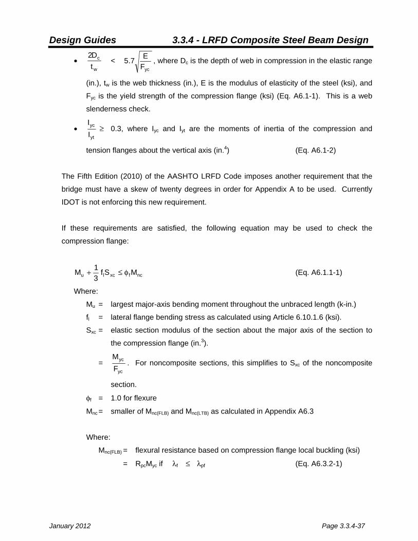
The provisions of Appendix A6 may only be used if the following requirements are satisfied:
• The bridge must be straight or equivalently straight according to the provisions of
(4.6.1.2.4b)
• The specified minimum yield strengths of the flanges and web do not exceed 70.0 ksi

Design Guides 3.3.4 - LRFD Composite Steel Beam Design
January 2012 Page 3.3.4-15
• w
c
tD2
< ycFE7.5 , where Dc is the depth of web in compression in the elastic range
(in.), tw is the web thickness (in.), E is the modulus of elasticity of the steel (ksi), and
Fyc is the yield strength of the compression flange (ksi) (Eq. A6.1-1). This is a web
slenderness check.
• yt
yc
II
≥ 0.3, where Iyc and Iyt are the moments of inertia of the compression and
tension flanges about the vertical axis (in.4) (Eq. A6.1-2)
The Fifth Edition (2010) of the AASHTO LRFD Code imposes another requirement that the
bridge must have a skew of twenty degrees in order for Appendix A to be used. Currently
IDOT is not enforcing this new requirement.
If these requirements are satisfied, the following equation may be used to check the
compression flange:
ncfxclu MSf31M φ≤+ (Eq. A6.1.1-1)
Where:
Mu = largest major-axis bending moment throughout the unbraced length (k-in.)
fl = lateral flange bending stress as calculated using Article 6.10.1.6 (ksi), taken as
zero for constructability loading.
Sxc = elastic section modulus of the section about the major axis of the section to
the compression flange (in.3).
= yc
yc
FM
. For noncomposite sections, this simplifies to Sxc of the noncomposite
section.
φf = 1.0 for flexure
Mnc = smaller of Mnc(FLB) and Mnc(LTB) as calculated in Appendix A6.3
Where:
Mnc(FLB) = flexural resistance based on compression flange local buckling (ksi)
= RpcMyc if λf ≤ λpf (Eq. A6.3.2-1)

Design Guides 3.3.4 - LRFD Composite Steel Beam Design
Page 3.3.4-16 January 2012
= ycpcpfrf
pff
ycpc
xcyr MRMRSF
11⎥⎥⎦
⎤
⎢⎢⎣
⎡⎟⎟⎠
⎞⎜⎜⎝
⎛
λ−λλ−λ
⎟⎟⎠
⎞⎜⎜⎝
⎛−− otherwise
(Eq. A6.3.2-2)
Where:
Fyr = compression flange stress at the onset of nominal yielding within the
cross section, taken as the smaller of 0.7Fyc, RhFytSxt / Sxc and Fyw
(yield strength of the web), but not smaller than 0.5Fyc.
Fyc = yield strength of the compression flange (ksi)
Fyt = yield strength of the tension flange (ksi)
Fyw = yield strength of the web (ksi)
Sxc = elastic section modulus of the section about the major axis of the
section to the compression flange (in.3).
= yc
yc
FM
. For noncomposite sections, this simplifies to Sxc of the
noncomposite section.
Myc = yield moment with respect to the compression flange. For
noncomposite sections, this is taken as SxcFyc. (k-in.)
λf = slenderness ratio of compression flange
= fc
fc
t2b (Eq. A6.3.2-3)
λpf = limiting slenderness ratio for a compact flange
= ycFE38.0 (Eq. A6.3.2-4)
λrf = limiting slenderness ratio for a noncompact flange
= yr
c
FEk
95.0 (Eq. A6.3.2-5)
kc =
wtD4 0.35 ≤ kc ≤ 0.76 for built-up sections (Eq. A6.3.2-6)
= 0.76 for rolled shapes
Rpc = web plastification factor

Design Guides 3.3.4 - LRFD Composite Steel Beam Design
January 2012 Page 3.3.4-17
= yc
p
MM
if w
cp
tD2
≤ λpw(Dcp) (Eq. A6.2.1-1)
= yc
p
)Dc(pwrw
)Dc(pww
p
ych
MM
MMR
11⎥⎥⎦
⎤
⎢⎢⎣
⎡⎟⎟⎠
⎞⎜⎜⎝
⎛
λ−λλ−λ
⎟⎟⎠
⎞⎜⎜⎝
⎛−− ≤
yc
p
MM
otherwise
(Eq. A6.2.2-4)
Where:
Mp = plastic moment determined as specified in Article D6.1 (k-in.)
Myc = FycSxc for noncomposite sections (k-in.)
Dcp = depth of web in compression at the plastic moment as specified in
Article D6.3.2 (k-in.)
λpw(Dcp) = limiting slenderness ratio for a compact web corresponding to
2Dcp / tw
= 2
yh
p
yc
09.0MR
M54.0
FE
⎟⎟⎠
⎞⎜⎜⎝
⎛−
≤ ⎟⎟⎠
⎞⎜⎜⎝
⎛λ
c
cprw D
D (Eq. A6.2.1-2)
λpw(Dc) = limiting slenderness ratio for a compact web corresponding to
2Dc / tw
= ⎟⎟⎠
⎞⎜⎜⎝
⎛λ
cp
c)Dcp(pw D
D≤ rwλ (Eq. A6.2.2-6)
λrw = ycF
E7.5 (Eq. A6.2.1-3)
Mnc(LTB) = flexural resistance based on lateral-torsional buckling (k-in.)
For Lb ≤ Lp:
Mnc(LTB) = RpcMyc (Eq. A6.3.3-1)
For Lp < Lb ≤ Lr:

Design Guides 3.3.4 - LRFD Composite Steel Beam Design
Page 3.3.4-18 January 2012
Mnc(LTB) = ycpcycpcpr
pb
ycpc
xcyrb MRMR
LLLL
MRSF
11C ≤⎥⎥⎦
⎤
⎢⎢⎣
⎡⎟⎟⎠
⎞⎜⎜⎝
⎛
−−
⎟⎟⎠
⎞⎜⎜⎝
⎛−−
(Eq. A6.3.3-2)
For Lb > Lr:
Mnc(LTB) = FcrSxc ≤ RpcMyc (Eq. A6.3.3-3)
Where:
Lb = unbraced length (in.)
Lp = yc
t FEr0.1 (Eq. A6.3.3-4)
Lr = 2
xcyr
xcyrt J
hSE
F76.611
hSJ
FEr95.1 ⎟⎟
⎠
⎞⎜⎜⎝
⎛++ (Eq. A6.3.3-5)
Where:
rt = effective radius of gyration for lateral-torsional buckling (in.)
=
⎟⎟⎠
⎞⎜⎜⎝
⎛+
fcfc
wc
fc
tbtD
31112
b (Eq. A6.3.3-10)
E = modulus of elasticity of steel (ksi)
Fyr = compression flange stress at onset of yielding, as
calculated in Mnc(FLB) calculations (ksi)
J = St. Venant’s torsional constant, taken as the sum of the
moments of inertia of all contributing members about their
major axes at the end of the member, with corrections
= ⎟⎟⎠
⎞⎜⎜⎝
⎛−+⎟⎟
⎠
⎞⎜⎜⎝
⎛−+
ft
ft3ftft
fc
fc3fcfc
3w
bt
63.013tb
bt
63.013tb
3Dt
(Eq. A6.3.3-9)
Sxc = elastic section modulus about the major axis of the section
to the compression flange. For noncomposite beams this is
Sxc of the noncomposite section. (in.3)
h = section depth (in.)
Design Guides 3.3.4 - LRFD Composite Steel Beam Design
January 2012 Page 3.3.4-19
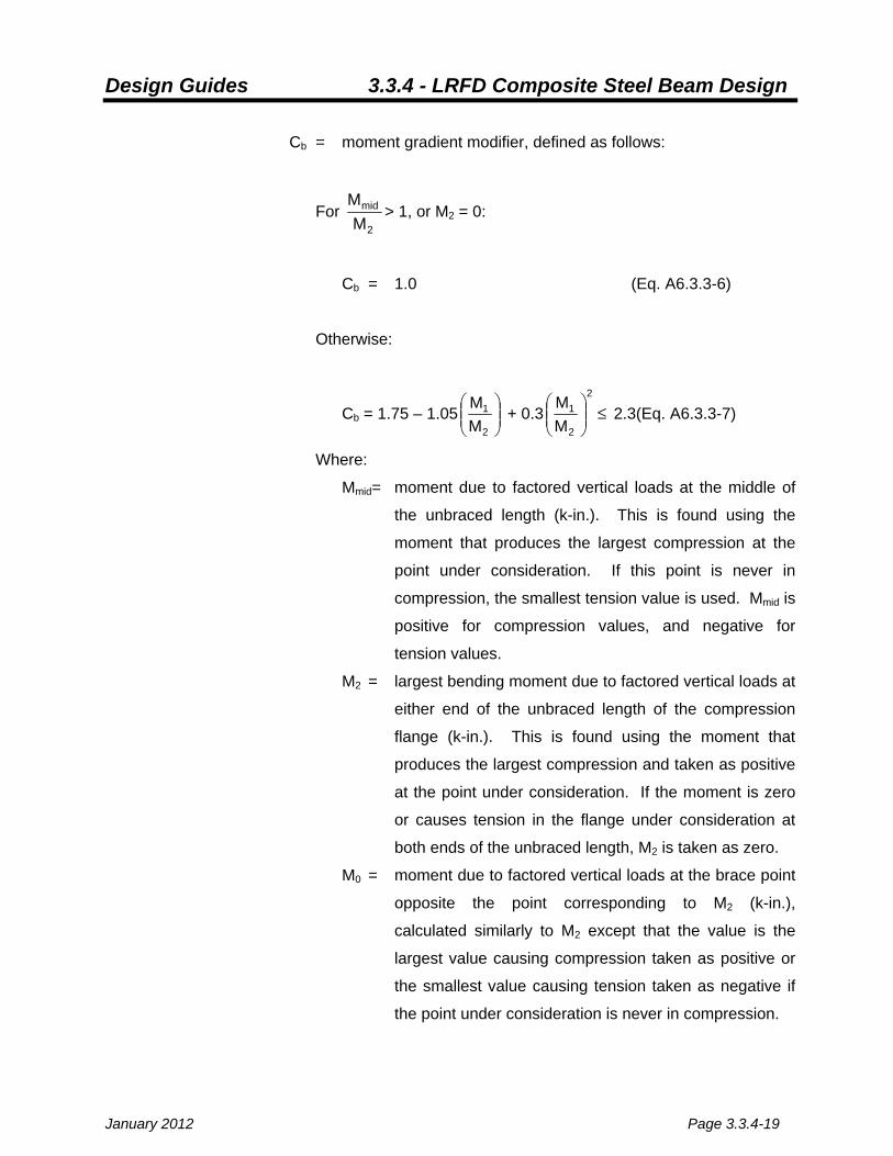
Cb = moment gradient modifier, defined as follows:
For 2
mid
MM
> 1, or M2 = 0:
Cb = 1.0 (Eq. A6.3.3-6)
Otherwise:
Cb = 1.75 – 1.05 ⎟⎟⎠
⎞⎜⎜⎝
⎛
2
1
MM
+ 0.32
2
1
MM
⎟⎟⎠
⎞⎜⎜⎝
⎛≤ 2.3(Eq. A6.3.3-7)
Where:
Mmid= moment due to factored vertical loads at the middle of
the unbraced length (k-in.). This is found using the
moment that produces the largest compression at the
point under consideration. If this point is never in
compression, the smallest tension value is used. Mmid is
positive for compression values, and negative for
tension values.
M2 = largest bending moment due to factored vertical loads at
either end of the unbraced length of the compression
flange (k-in.). This is found using the moment that
produces the largest compression and taken as positive
at the point under consideration. If the moment is zero
or causes tension in the flange under consideration at
both ends of the unbraced length, M2 is taken as zero.
M0 = moment due to factored vertical loads at the brace point
opposite the point corresponding to M2 (k-in.),
calculated similarly to M2 except that the value is the
largest value causing compression taken as positive or
the smallest value causing tension taken as negative if
the point under consideration is never in compression.

Design Guides 3.3.4 - LRFD Composite Steel Beam Design
Page 3.3.4-20 January 2012
M1 = moment at the brace point opposite to the one
corresponding to M2, calculated as the intercept of the
most critical assumed linear moment variation passing
through M2 and either Mmid or M0, whichever produces
the smallest value of Cb (k-in.). M1 may be determined
as follows:
When the variation of the moment along the entire
length between the brace points is concave:
M1 = M0 (Eq. A6.3.3-11)
Otherwise:
M1 = 2Mmid – M2 ≥ M0 (Eq. A6.3.3-12)
Fcr = elastic lateral-torsional buckling stress (ksi)
= 2
t
b
xc2
t
b
2b
rL
hSJ078.01
rL
EC⎟⎟⎠
⎞⎜⎜⎝
⎛+
⎟⎟⎠
⎞⎜⎜⎝
⎛
π (Eq. A6.3.3-8)
Check Discretely Braced Tension Flanges (Appendix A) (A6.4)
The nominal flexural resistance based on tension flange yielding is taken as:
Mnt = RptMyt (Eq. A6.4-1)
Where Rpt and Myt are calculcated similar to Rpc and Myc above.
Additional Constructibility Checks
Articles 6.10.3.2.4, 6.10.3.4, and 6.10.3.5 involve consideration of issues arising from bridges
with pouring sequences, staged construction, loading sequences during construction, etc.
For a particular typical bridge, these articles may or may not apply. The commentaries,

Design Guides 3.3.4 - LRFD Composite Steel Beam Design
January 2012 Page 3.3.4-21
however, provide useful guidance to the engineer. Article 6.10.3.3 examines shear forces in
webs during construction loading. As the final Strength I shears are usually much greater
than construction loading shears, this generally does not control the design.
Check Service Limit State (6.10.4)
The purpose of the service limit state requirements are to prevent excessive deflections
(possibly from yielding or slip in connections) due to severe traffic loading in a real-life
situation. Service II load factors are used for these checks: the actual dead loads are
applied (load factor of 1.00), along with 1.3 times the projected live load plus impact.
IISERVICEM = 1.00(DC1 + DC2)+1.00(DW)+1.30(LL+IM) (Table 3.4.1-1)
For this load case, the following flange requirements shall be met:
The top steel flange of composite sections shall satisfy:
( ) ( )yfhf FR95.0f ≤ (Eq. 6.10.4.2.2-1)
Note that “top steel flange” in this case is referring to the flange adjacent to the deck and
not necessarily the compression flange. This equation does not include the lateral flange
stress term because for flanges attached to decks with studs fl is assumed to be zero.
This equation need not be checked for composite sections in negative flexure if 6.10.8 is
used to calculate the ultimate capacity of the section. It also need not be checked for
noncompact composite sections in positive flexure (C6.10.4.2.2).
The bottom steel flange of composite sections shall satisfy:
( ) ( )yfhl
f FR95.02ff ≤+ (Eq. 6.10.4.2.2-2)
Where:

Design Guides 3.3.4 - LRFD Composite Steel Beam Design
Page 3.3.4-22 January 2012
ff = flange stress due to factored vertical Service II loads (ksi), calculated as
follows:
For positive moment regions:
ff = ( )9n
IMLL
27n
DW2DC
nc
1DC
SM3.1
SMM
SM
=
+
=
+++ (Eq. D6.2.2-1)
For negative moment regions:
Article 6.10.4.2.1 allows for an uncracked section if the stresses in the slab are less
than twice the modulus of rupture of the concrete. Therefore:
ff = ( )
9n
IMLL
27n
DW2DC
nc
1DC
SM3.1
SMM
SM
=
+
=+
++ if fslab< 2fr (Eq. D6.2.2-1)
ff = ( )cr,c
IMLLDW2DC
nc
1DC
SM3.1MM
SM +++
+ if fslab> 2fr (Eq. D6.2.2-1)
Where:
MDC1 = moment due to dead loads on noncomposite section. Typically this
consists of the dead loads due to the steel beam and the weight of the
concrete deck and fillet (k-in.)
MDC2 = moment due to dead loads on composite section. Typically this
consists of the dead loads due to parapets, sidewalks, railings, and
other appurtenances (k-in.)
MDW = moment due to the future wearing surface (k-in.)
MLL+IM = moment due to live load plus impact (k-in.)
Snc = section modulus of noncomposite section about the major axis of
bending to the flange being checked (in.3)
Sn=27 = section modulus of long-term composite section about the major axis
of bending to the flange being checked (deck transposed by a factor of
3n = 27) (in.3)

Design Guides 3.3.4 - LRFD Composite Steel Beam Design
January 2012 Page 3.3.4-23
Sn=9 = section modulus of short-term composite section about the major axis
of bending to the flange being checked (deck transposed by a factor of
n = 9) (in.3)
Sc,cr = section modulus of steel section plus longitudinal deck reinforcement
about the major axis of bending to the flange being checked (cracked
composite section) (in.3)
fslab = stress at top of deck during Service II loading assuming an uncracked
section (ksi). Note that when checking the concrete deck stresses, a
composite section transformed to concrete should be used (as
opposed to a composite section transformed to steel). This is done by
multiplying the section moduli by their respective transformation ratios.
Adding these transformation ratios to stress equations, the deck stress
is found as follows:
= ( )⎟⎟⎠
⎞⎜⎜⎝
⎛+⎟⎟
⎠
⎞⎜⎜⎝
⎛ +
=
+
= 9n
IMLL
27n
DW2DC
SM3.1
n1
SMM
n31
fr = modulus of rupture of concrete (ksi)
= c'f24.0
Again, for straight interior beams with skews less than or equal to 45°, fl can be
assumed to be zero.
Sections in positive flexure with D / tw > 150, and all sections in negative flexure designed
using Appendix A for Strength I design shall also satisfy the following requirement:
fc < Fcrw (Eq. 6.10.4.2.2-4)
Where:
fc = stress in the bottom flange in the negative moment region, calculated as ff
above (ksi)
Fcrw = nominal web bend-buckling resistance
= 2
wtD
Ek9.0
⎟⎟⎠
⎞⎜⎜⎝
⎛ < RhFyc and Fyw / 0.7 (Eq. 6.10.1.9.1-1)

Design Guides 3.3.4 - LRFD Composite Steel Beam Design
Page 3.3.4-24 January 2012
Where:
E = modulus of elasticity of steel (ksi)
D = total depth of web (in.)
tw = web thickness (in.)
Rh = hybrid factor as stated above
Fyc = yield strength of compression flange (ksi)
Fyw = yield strength of web (ksi)
k = 2c
DD
9
⎟⎟⎠
⎞⎜⎜⎝
⎛ (Eq. 6.10.1.9.1-2)
Where:
Dc = depth of web in compression, calculated in accordance with Appendix
D6.3.1.
Equation 6.10.4.2.2-3 is only necessary for sections noncomposite in final loading. As it is
IDOT practice is to provide shear stud connectors along the entire length of bridges, this
equation is not applicable. As stated in Section 3.3.2 of the Bridge Manual, the live load
deflection and span-to-depth ratio provisions of Article 2.5.2.6.2, referenced by Article
6.10.4.1, are only applicable to bridges with pedestrian traffic.
The code provisions in 6.10.4.2.2 reference Appendix B6, which allows for moment
redistribution. This is not allowed by the Department.
Check Fatigue and Fracture Limit State (6.10.5)
Fatigue and fracture limit state requirements are necessary to prevent beams and
connections from failing due to repeated loadings.
For the fatigue load combination, all moments are calculated using the fatigue truck specified
in Article 3.6.1.4. The fatigue truck is similar to the HL-93 truck, but with a constant 30 ft. rear
axle spacing. Lane loading is not applied. The fatigue truck loading uses a different
Dynamic Load Allowance of 15% (Table 3.6.2.1-1).

Design Guides 3.3.4 - LRFD Composite Steel Beam Design
January 2012 Page 3.3.4-25
Note: The fatigue truck loading does not use multiple presence factors. The value of the live
load distribution factor must be divided by 1.2 when finding moments from the fatigue truck
(3.6.1.1.2).
The fatigue and fracture limit state uses the fatigue load combinations found in Table 3.4.1-1:
MFATIGUE I = 1.5(LL+IM+CE) (Table 3.4.1-1)
MFATIGUE II = 0.75(LL+IM+CE) (Table 3.4.1-1)
Whether Fatigue I or Fatigue II limit state is used depends upon the amount of fatigue cycles
the member is expected to experience throughout its lifetime. For smaller amounts of cycles,
Fatigue II, or the finite life limit state, is used. As the amounts of cycles increase, there
comes a point where use of finite life limit state equations becomes excessively conservative,
and use of the Fatigue I, or infinite life limit state, becomes more accurate.
To determine whether Fatigue I or Fatigue II limit state is used, the single-lane average daily
truck traffic (ADTT)SL at 75 years must first be calculated. (ADTT)SL is the amount of truck
traffic in a single lane in one direction, taken as a reduced percentage of the Average Daily
Truck Traffic (ADTT) for multiple lanes of travel in one direction.
(ADTT)75, SL = p × ADTT75 (Eq. 3.6.1.4.2-1)
Where:
p = percentage of truck traffic in a single lane in one direction, taken from Table
3.6.1.4.2-1.
ADTT75 is the amount of truck traffic in one direction of the bridge at 75 years. Type,
Size, and Location reports usually give ADTT in terms of present day and 20 years
into the future. The ADTT at 75 years can be extrapolated from this data by
assuming that the ADTT will grow at the same rate i.e. follow a straight-line
extrapolation using the following formula:
ADTT75 = ( ) ( )DDADTTyears20years57ADTTADTT 0020 ⎟⎟
⎠
⎞⎜⎜⎝
⎛+⎟⎟
⎠
⎞⎜⎜⎝
⎛−

Design Guides 3.3.4 - LRFD Composite Steel Beam Design
Page 3.3.4-26 January 2012
Where:
ADTT20 = ADTT at 20 years in the future, given on TSL
ADTT0 = present-day ADTT, given on TSL
DD = directional distribution, given on TSL
The designer should use the larger number given in the directional distribution. For
example, if the directional distribution of traffic was 70% / 30%, the ADTT for design
should be the total volume times 0.7 in order to design for the beam experiencing the
higher ADTT. If a bridge has a directional distribution of 50% / 50%, the ADTT for
design should be the total volume times 0.5. If a bridge is one-directional, the ADTT
for design is the full value, as the directional distribution is 100% / 0% i.e. one.
When (ADTT)75, SL is calculated, it is compared to the infinite life equivalent found in Table
6.6.1.2.3-2. If the calculated value of (ADTT)75, SL exceeds the value found in this table, then
the infinite life (Fatigue I) limit state is used. If not, the finite life (Fatigue II) limit state is used.
Regardless of limit state, the full section shall satisfy the following equation:
( ) ( )nFf Δ≤Δγ (Eq. 6.6.1.2.2-1)
Where:
γ = Fatigue load factor, specified in Table 3.4.1-1
( )fΔ = Fatigue load combination stress range (ksi)
= 9n
FATIGUEFATIGUE
SMM
=
−+ −
Currently, the effects of lateral flange bending stress need not be considered
in the check of fatigue.
( )nFΔ = nominal fatigue resistance (ksi), found as follows:
For Fatigue I limit state:
( )nFΔ = ( )THFΔ (Eq. 6.6.1.2.5-1)

Design Guides 3.3.4 - LRFD Composite Steel Beam Design
January 2012 Page 3.3.4-27
Where ( )THFΔ is the threshold stress range found in Table 6.6.1.2.3-1 or Table
6.6.1.2.5-3 (ksi)
For Fatigue II limit state:
( )nFΔ = 31
NA⎟⎠⎞
⎜⎝⎛ (Eq. 6.6.1.2.5-2)
Where:
A = constant from Table 6.6.1.2.3-1 or Table 6.6.1.2.5-1 (ksi3). For typical
painted rolled sections and painted plate girders:
• Fatigue category A should be used in positive moment regions
• Fatigue Category C should be used in negative moment regions to
account for the effect of the studs (See Descriptions 1.1 and 8.1 in
Table 6.6.1.2.3-1).
For typical rolled sections and plate girders made of weathering steel:
• Fatigue Category B should be used in positive moment regions
• Fatigue Category C should be used in negative moment regions
(See Descriptions 1.2 and 8.1 in Table 6.6.1.2.3-1).
For plate girders, brace points should also be checked for category C’
(See Description 4.1).
N = ( ) ⎟⎟⎠
⎞⎜⎜⎝
⎛⎟⎠⎞
⎜⎝⎛
⎟⎟⎠
⎞⎜⎜⎝
⎛day
trucks)ADTT(truckcyclesnyears75
yeardays365 SL,5.37
(Eq. 6.6.1.2.5-3)
Where:
n = number of stress cycles per truck passage, taken from
Table 6.6.1.2.5-2
(ADTT)37.5, SL = single lane ADTT at 37.5 years. This is calculated in a
similar fashion as the calculation of (ADTT)75, SL above
except that the multiplier 37.5/20 is used in place of the
multiplier 75/20 when extrapolating.

Design Guides 3.3.4 - LRFD Composite Steel Beam Design
Page 3.3.4-28 January 2012
Additionally, all rolled sections shall satisfy the Temperature Zone 2 Charpy V-notch fracture
toughness requirements of Article 6.6.2. See also Section 3.3.7 of the Bridge Manual.
Interior panels of stiffened webs in negative moment regions shall also satisfy the shear
requirements of 6.10.9.3.3. See 6.10.5.3. This section is similar to that discussed in the
Check Strength Limit State (Shear) portion of this design guide.
Many typical bridges made with rolled steel sections need not satisfy the requirements of
distortion-induced fatigue given in Article 6.6.1.3. This can become a consideration for
bridges with high skews, curved members, etc.
Check Strength Limit State (Moment) (6.10.6)
Strength limit state compares the ultimate shear and moment capacities of the sections to the
factored Strength I loads applied to the bridge. Strength I factors for this limit state are as
follows:
MSTRENGTH I = γp(DC+DW)+1.75(LL+IM+CE)
Where:
γp = For DC: 1.25 max., 0.9 min. (Table 3.4.1-2)
For DW: 1.50 max., 0.65 min..
For single-span bridges, use the maximum values of γp in all locations.
Positive Moment Regions
Composite positive moment regions are checked using Chapter 6 only. Appendix A6 does
not apply to composite positive moment regions.
The strength limit state requirements for compact sections differ from those for
noncompact sections. Compact rolled sections are defined in Article 6.10.6.2.2 as
sections that satisfy the following:
Design Guides 3.3.4 - LRFD Composite Steel Beam Design
January 2012 Page 3.3.4-29
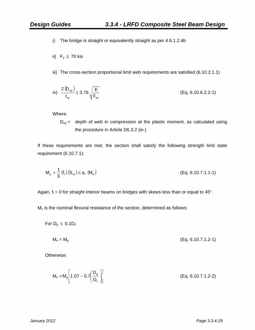
i) The bridge is straight or equivalently straight as per 4.6.1.2.4b
ii) Fy ≤ 70 ksi
iii) The cross-section proportional limit web requirements are satisfied (6.10.2.1.1)
iv) ( )
ycw
cp
FE76.3
tD2
≤ (Eq. 6.10.6.2.2-1)
Where:
Dcp = depth of web in compression at the plastic moment, as calculated using
the procedure in Article D6.3.2 (in.)
If these requirements are met, the section shall satisfy the following strength limit state
requirement (6.10.7.1):
( ) ( ) ( )nfxtlu MSf31M φ≤+ (Eq. 6.10.7.1.1-1)
Again, fl = 0 for straight interior beams on bridges with skews less than or equal to 45°.
Mn is the nominal flexural resistance of the section, determined as follows:
For Dp ≤ 0.1Dt:
Mn = Mp (Eq. 6.10.7.1.2-1)
Otherwise:
Mn =⎥⎥⎦
⎤
⎢⎢⎣
⎡⎟⎟⎠
⎞⎜⎜⎝
⎛−
t
pp D
D7.007.1M (Eq. 6.10.7.1.2-2)

Design Guides 3.3.4 - LRFD Composite Steel Beam Design
Page 3.3.4-30 January 2012
Where:
Dp = distance from the top of the concrete deck to the neutral axis of the
composite section at the plastic moment (in.)
Dt = total depth of the composite section (in.)
Mp = plastic moment capacity (k-in.) of the composite section calculated using
the procedure in Article D6.1
For continuous spans, the following requirement also applies:
Mn ≤ 1.3RhMy (Eq. 6.10.7.1.2-3)
Where:
Rh = hybrid factor, taken as 1.0 for non-hybrid sections (sections with the same
grade of steel in the webs and flanges)
My = controlling yield moment of section (k-in.). In composite positive moment
regions, the controlling yield moment will likely be governed by the bottom
flange.
= 9n,c27n,c
DW2DC
nc
1DCyfDW2DC1DC S
SMM
SM
FM5.1M25.1M25.1 ==
⎟⎟⎠
⎞⎜⎜⎝
⎛ +−−+++
(Eq. D6.2.2-1 and 2)
The purpose of this check is to ensure that the plastic moment capacity does not exceed
the yield strength by too large a margin. If this were to happen, significant changes in
stiffness may occur in the beam during yielding. These changes in stiffness can result in
redistribution of moments, resulting in non-conservative designs in different parts of the
bridge.
If the beam does not meet the compactness criteria listed above, it is noncompact and shall
satisfy the following equations:
fbu ≤ φfFnc (compression flanges) (Eq. 6.10.7.2.1-1)
ntflbu Ff31f φ≤+ (tension flanges) (Eq. 6.10.7.2.1-2)

Design Guides 3.3.4 - LRFD Composite Steel Beam Design
January 2012 Page 3.3.4-31
Where:
fbu = flange stress calculated without consideration of lateral bending stresses (ksi)
φf = 1.0 for flexure
fl = lateral flange bending stress (ksi)
Fnc = RbRhFyc (Eq. 6.10.7.2.2-1)
Fnt = RhFyt (Eq. 6.10.7.2.2-2)
Where:
Rb = web load-shedding factor. In most cases this is assumed to be 1.0
(6.10.1.10.2). However, there are cases involving slender webs (not
satisfying the cross-section proportion limits of 6.10.2.1.1) that also have a
shallow depth of web in compression where Rb need be calculated. In
these cases, the provisions of 6.10.1.10.2 shall be followed. However, this
is not typical in IDOT bridges and will not be outlined in this design guide.
Rh = hybrid factor, taken as 1.0 for non-hybrid sections (sections with the same
grade of steel in the web and flanges)
Fyc = yield strength of compression flange (ksi)
Fyt = yield strength of tension flange (ksi)
Regardless of whether or not the section is compact, it shall satisfy the following ductility
requirement:
Dp ≤ 0.42Dt (Eq. 6.10.7.3-1)
This check is analogous to checking a reinforced concrete beam for c/d < 0.42 (see
C5.7.2.1). The purpose is to prevent the concrete slab eccentricity from becoming too large,
resulting in a section where concrete will crush in order to maintain compatibility with the
yielding steel.
Negative Moment Regions
Composite negative moment regions may be checked using either the provisions of Chapter
6 or, if applicable, the provisions of Appendix A6. Use of provisions of Appendix A6 is
encouraged when applicable. This design guide will outline the use of both sets of equations.

Design Guides 3.3.4 - LRFD Composite Steel Beam Design
Page 3.3.4-32 January 2012
Check Discretely Braced Compression Flanges (Chapter 6) (6.10.8.1.1)
In this check, the applied compression flange stress is checked against the local flange
buckling stress and the lateral-torsional buckling stress. Both of these stresses are based
upon Fy of the compression flange, so a comparison to the yield strength of the compression
flange is inherent in this check and is not a separate check, as it is when checking
constructibility.
ncflbu Ff31f φ≤+ (Eq. 6.10.8.1.1-1)
Where:
fbu = factored flange stress due to vertical loads (ksi)
= 9n,c
IMLL
27n,c
DW2DC
nc
1DC
SM75.1
SM5.1M25.1
SM25.1
=
+
=+
++
fl = lateral flange bending stress (ksi) due to cantilever forming brackets and skew
effects. Note that this term should typically be taken as zero for a majority of
typical bridges if the requirements of Article 503.06 of the IDOT Standard
Specifications are met and the bridge skew is less than or equal to 45°. See
also Sections 3.3.5 and 3.3.26 of the Bridge Manual.
φf = resistance factor for flexure, equal to 1.00 according to LRFD Article 6.5.4.2
Fnc = nominal flexural resistance of the flange (ksi), taken as the lesser Fnc(FLB)
(6.10.8.2.2) and Fnc(LTB) (6.10.8.2.3).
Where:
Fnc(FLB) = Flange Local Buckling resistance (ksi), specified in Article 6.10.8.2.2,
defined as follows:
For λf ≤ λpf:
Fnc(FLB) = RbRhFyc (Eq. 6.10.8.2.2-1)
Otherwise:

Design Guides 3.3.4 - LRFD Composite Steel Beam Design
January 2012 Page 3.3.4-33
Fnc(FLB) = ychbpfrf
pff
ych
yr FRRFR
F11
⎥⎥⎦
⎤
⎢⎢⎣
⎡⎟⎟⎠
⎞⎜⎜⎝
⎛
λ−λλ−λ
⎟⎟⎠
⎞⎜⎜⎝
⎛−− (Eq. 6.10.8.2.2-2)
Where:
Fyc = compression flange stress at the onset of nominal yielding
within the cross section, taken as the smaller of 0.7Fyc and
Fyw (yield strength of the web), but not smaller than 0.5Fyc.
λf = slenderness ratio of compression flange
= fc
fc
t2b (Eq. 6.10.8.2.2-3)
λpf = limiting slenderness ratio for a compact flange
= ycFE38.0 (Eq. 6.10.8.2.2-4)
λrf = limiting slenderness ratio for a noncompact flange
= yrFE56.0 (Eq. 6.10.8.2.2-5)
Rb = web load-shedding factor, specified in Article 6.10.1.10.2,
typically assumed to be 1.0 for cases that meet the cross-
section proportion limits of 6.10.2. See above for further
discussion.
Fnc(LTB) = Lateral-Torsional Buckling Resistance (ksi), specified in Article
6.10.8.2.3. For the purposes of calculating Fnc(LTB), variables Lb, Lp,
and Lr, are defined as follows:
Lb = unbraced length (in.)
Lp = limiting unbraced length to achieve nominal flexural resistance
under uniform bending (in.)
= yc
t FEr0.1 (Eq. 6.10.8.2.3-4)
Lr = limiting unbraced length for inelastic buckling behavior under
uniform bending (in.)

Design Guides 3.3.4 - LRFD Composite Steel Beam Design
Page 3.3.4-34 January 2012
= yr
t FErπ (Eq. 6.10.8.2.3-5)
Where:
rt =
⎟⎟⎠
⎞⎜⎜⎝
⎛+
fcfc
wc
fc
tbtD
31112
b (Eq. 6.10.8.2.3-9)
Dc = depth of web in compression, calculated according to Article
D6.3.1.
Fnc(LTB) is then calculated as follows:
For Lb ≤ Lp:
Fnc(LTB) = RbRhFyc (Eq. 6.10.8.2.3-1)
For Lp < Lb ≤ Lr:
Fnc(LTB) = ychbychbpr
pb
ych
yrb FRRFRR
LLLL
FRF
11C ≤⎥⎥⎦
⎤
⎢⎢⎣
⎡⎟⎟⎠
⎞⎜⎜⎝
⎛
−−
⎟⎟⎠
⎞⎜⎜⎝
⎛−−
(Eq. 6.10.8.2.3-2)
For Lb > Lr:
Fnc = Fcr ≤ RbRhFyc (Eq. 6.10.8.2.3-3)
Where:
Fyr = as defined above
Fcr = elastic lateral-torsional buckling stress (ksi)
= 2
t
b
2bb
rL
ERC
⎟⎟⎠
⎞⎜⎜⎝
⎛
π (Eq. 6.10.8.2.3-8)

Design Guides 3.3.4 - LRFD Composite Steel Beam Design
January 2012 Page 3.3.4-35
Where:
Cb = moment gradient modifier, defined as follows:
For 2
mid
ff
> 1, or f2 = 0:
Cb = 1.0 (Eq. 6.10.8.2.3-6)
Otherwise:
Cb = 1.75 – 1.05 ⎟⎟⎠
⎞⎜⎜⎝
⎛
2
1
ff
+ 0.32
2
1
ff⎟⎟⎠
⎞⎜⎜⎝
⎛≤ 2.3 (Eq. 6.10.8.2.3-7)
Where:
fmid = stress due to factored vertical loads at the middle of
the unbraced length of the compression flange (ksi).
This is found using the moment that produces the
largest compression at the point under
consideration. If this point is never in compression,
the smallest tension value is used. fmid is positive for
compression values, and negative for tension
values.
f2 = largest compressive stress due to factored vertical
loads at either end of the unbraced length of the
compression flange (ksi). This is found using the
moment that produces the largest compression and
taken as positive at the point under consideration. If
the stress is zero or tensile in the flange under
consideration at both ends of the unbraced length, f2
is taken as zero.
f0 = stress due to factored vertical loads at the brace
point opposite the point corresponding to f2 (ksi),
calculated similarly to f2 except that the value is the
largest value in compression taken as positive or the

Design Guides 3.3.4 - LRFD Composite Steel Beam Design
Page 3.3.4-36 January 2012
smallest value in tension taken as negative if the
point under consideration is never in compression.
f1 = stress at the brace point opposite to the one
corresponding to f2, calculated as the intercept of the
most critical assumed linear stress variation passing
through f2 and either fmid or f0, whichever produces
the smallest value of Cb (ksi). f1 may be determined
as follows:
When the variation of the moment along the entire
length between the brace points is concave:
f1 = f0 (Eq. 6.10.8.2.3-10)
Otherwise:
f1 = 2fmid – f2 ≥ f0 (Eq. 6.10.8.2.3-11)
Check Continuously Braced Tension Flanges (Chapter 6) (6.10.8.1.3)
yfhfbu FRf φ≤ (Eq. 6.10.8.1.3-1)
Where all variables and assumptions are identical to those used for checking the
compression flange.
Check Discretely Braced Compression Flanges (Appendix A6) (A6.1.1)
The provisions of Appendix A6 may only be used if the following requirements are satisfied:
• The bridge must be straight or equivalently straight according to the provisions of
(4.6.1.2.4b)
• The specified minimum yield strengths of the flanges and web do not exceed 70.0 ksi
Design Guides 3.3.4 - LRFD Composite Steel Beam Design
January 2012 Page 3.3.4-37
• w
c
tD2
< ycFE7.5 , where Dc is the depth of web in compression in the elastic range
(in.), tw is the web thickness (in.), E is the modulus of elasticity of the steel (ksi), and
Fyc is the yield strength of the compression flange (ksi) (Eq. A6.1-1). This is a web
slenderness check.
• yt
yc
II
≥ 0.3, where Iyc and Iyt are the moments of inertia of the compression and
tension flanges about the vertical axis (in.4) (Eq. A6.1-2)
The Fifth Edition (2010) of the AASHTO LRFD Code imposes another requirement that the
bridge must have a skew of twenty degrees in order for Appendix A to be used. Currently
IDOT is not enforcing this new requirement.
If these requirements are satisfied, the following equation may be used to check the
compression flange:
ncfxclu MSf31M φ≤+ (Eq. A6.1.1-1)
Where:
Mu = largest major-axis bending moment throughout the unbraced length (k-in.)
fl = lateral flange bending stress as calculated using Article 6.10.1.6 (ksi).
Sxc = elastic section modulus of the section about the major axis of the section to
the compression flange (in.3).
= yc
yc
FM
. For noncomposite sections, this simplifies to Sxc of the noncomposite
section.
φf = 1.0 for flexure
Mnc = smaller of Mnc(FLB) and Mnc(LTB) as calculated in Appendix A6.3
Where:
Mnc(FLB) = flexural resistance based on compression flange local buckling (ksi)
= RpcMyc if λf ≤ λpf (Eq. A6.3.2-1)

Design Guides 3.3.4 - LRFD Composite Steel Beam Design
Page 3.3.4-38 January 2012
= ycpcpfrf
pff
ycpc
xcyr MRMRSF
11⎥⎥⎦
⎤
⎢⎢⎣
⎡⎟⎟⎠
⎞⎜⎜⎝
⎛
λ−λλ−λ
⎟⎟⎠
⎞⎜⎜⎝
⎛−− otherwise
(Eq. A6.3.2-2)
Where:
Fyr = compression flange stress at the onset of nominal yielding within the
cross section, taken as the smaller of 0.7Fyc, RhFytSxt / Sxc and Fyw
(yield strength of the web), but not smaller than 0.5Fyc.
Fyc = yield strength of the compression flange (ksi)
Fyt = yield strength of the tension flange (ksi)
Fyw = yield strength of the web (ksi)
Sxt = elastic section modulus of the section about the major axis of the
section to the tension flange (in.3).
= yt
yt
FM
.
Sxc = elastic section modulus of the section about the major axis of the
section to the compression flange (in.3).
= yc
yc
FM
.
Myc = yield moment with respect to the compression flange, calculated in
accordance with Appendix D6.2.
λf = slenderness ratio of compression flange
= fc
fc
t2b (Eq. A6.3.2-3)
λpf = limiting slenderness ratio for a compact flange
= ycFE38.0 (Eq. A6.3.2-4)
λrf = limiting slenderness ratio for a noncompact flange
= yr
c
FEk
95.0 (Eq. A6.3.2-5)
kc =
wtD4 0.35 ≤ kc ≤ 0.76 for built-up sections (Eq. A6.3.2-6)

Design Guides 3.3.4 - LRFD Composite Steel Beam Design
January 2012 Page 3.3.4-39
= 0.76 for rolled shapes
Rpc = web plastification factor
= yc
p
MM
if w
cp
tD2
≤ λpw(Dcp) (Eq. A6.2.1-1)
= yc
p
)Dc(pwrw
)Dc(pww
p
ych
MM
MMR
11⎥⎥⎦
⎤
⎢⎢⎣
⎡⎟⎟⎠
⎞⎜⎜⎝
⎛
λ−λλ−λ
⎟⎟⎠
⎞⎜⎜⎝
⎛−− ≤
yc
p
MM
otherwise
(Eq. A6.2.2-4)
Where:
Mp = plastic moment determined as specified in Article D6.1 (k-in.)
Myc = FycSxc for noncomposite sections (k-in.)
Dcp = depth of web in compression at the plastic moment as specified in
Article D6.3.2 (k-in.)
λpw(Dcp) = limiting slenderness ratio for a compact web corresponding to
2Dcp / tw
= 2
yh
p
yc
09.0MR
M54.0
FE
⎟⎟⎠
⎞⎜⎜⎝
⎛−
≤ ⎟⎟⎠
⎞⎜⎜⎝
⎛λ
c
cprw D
D (Eq. A6.2.1-2)
λpw(Dc) = limiting slenderness ratio for a compact web corresponding to
2Dc / tw
= ⎟⎟⎠
⎞⎜⎜⎝
⎛λ
cp
c)Dcp(pw D
D≤ rwλ (Eq. A6.2.2-6)
λrw = ycF
E7.5 (Eq. A6.2.1-3)
Mnc(LTB) = flexural resistance based on lateral-torsional buckling (k-in.)
For Lb ≤ Lp:
Mnc(LTB) = RpcMyc (Eq. A6.3.3-1)
For Lp < Lb ≤ Lr:

Design Guides 3.3.4 - LRFD Composite Steel Beam Design
Page 3.3.4-40 January 2012
Mnc(LTB) = ycpcycpcpr
pb
ycpc
xcyrb MRMR
LLLL
MRSF
11C ≤⎥⎥⎦
⎤
⎢⎢⎣
⎡⎟⎟⎠
⎞⎜⎜⎝
⎛
−−
⎟⎟⎠
⎞⎜⎜⎝
⎛−−
(Eq. A6.3.3-2)
For Lb > Lr:
Mnc(LTB) = FcrSxc ≤ RpcMyc (Eq. A6.3.3-3)
Where:
Lb = unbraced length (in.)
Lp = yc
t FEr0.1 (Eq. A6.3.3-4)
Lr = 2
xcyr
xcyrt J
hSE
F76.611
hSJ
FEr95.1 ⎟⎟
⎠
⎞⎜⎜⎝
⎛++ (Eq. A6.3.3-5)
Where:
rt = effective radius of gyration for lateral-torsional buckling (in.)
=
⎟⎟⎠
⎞⎜⎜⎝
⎛+
fcfc
wc
fc
tbtD
31112
b (Eq. A6.3.3-10)
E = modulus of elasticity of steel (ksi)
Fyr = compression flange stress at onset of yielding, as
calculated in Mnc(FLB) calculations (ksi)
J = St. Venant’s torsional constant, taken as the sum of the
moments of inertia of all contributing members about their
major axes at the end of the member, with corrections
= ⎟⎟⎠
⎞⎜⎜⎝
⎛−+⎟⎟
⎠
⎞⎜⎜⎝
⎛−+
ft
ft3ftft
fc
fc3fcfc
3w
bt
63.013tb
bt
63.013tb
3Dt
(Eq. A6.3.3-9)
Sxc = elastic section modulus about the major axis of the section
to the compression flange. For noncomposite beams this is
Sxc of the noncomposite section. (in.3)
h = depth between centerlines of flanges (in.)

Design Guides 3.3.4 - LRFD Composite Steel Beam Design
January 2012 Page 3.3.4-41
Cb = moment gradient modifier, defined as follows:
For 2
mid
MM
> 1, or M2 = 0:
Cb = 1.0 (Eq. A6.3.3-6)
Otherwise:
Cb = 1.75 – 1.05 ⎟⎟⎠
⎞⎜⎜⎝
⎛
2
1
MM
+ 0.32
2
1
MM
⎟⎟⎠
⎞⎜⎜⎝
⎛≤ 2.3 (Eq. A6.3.3-7)
Where:
Mmid= moment due to factored vertical loads at the middle of
the unbraced length (k-in.). This is found using the
moment that produces the largest compression at the
point under consideration. If this point is never in
compression, the smallest tension value is used. Mmid is
positive for compression values, and negative for
tension values.
M2 = largest bending moment due to factored vertical loads at
either end of the unbraced length of the compression
flange (k-in.). This is found using the moment that
produces the largest compression and taken as positive
at the point under consideration. If the moment is zero
or causes tension in the flange under consideration at
both ends of the unbraced length, M2 is taken as zero.
M0 = moment due to factored vertical loads at the brace point
opposite the point corresponding to M2 (k-in.),
calculated similarly to M2 except that the value is the
largest value causing compression taken as positive or
the smallest value causing tension taken as negative if
the point under consideration is never in compression.
M1 = moment at the brace point opposite to the one
corresponding to M2, calculated as the intercept of the

Design Guides 3.3.4 - LRFD Composite Steel Beam Design
Page 3.3.4-42 January 2012
most critical assumed linear moment variation passing
through M2 and either Mmid or M0, whichever produces
the smallest value of Cb (k-in.). M1 may be determined
as follows:
When the variation of the moment along the entire
length between the brace points is concave:
M1 = M0 (Eq. A6.3.3-11)
Otherwise:
M1 = 2Mmid – M2 ≥ M0 (Eq. A6.3.3-12)
Fcr = elastic lateral-torsional buckling stress (ksi)
= 2
t
b
xc2
t
b
2b
rL
hSJ078.01
rL
EC⎟⎟⎠
⎞⎜⎜⎝
⎛+
⎟⎟⎠
⎞⎜⎜⎝
⎛
π (Eq. A6.3.3-8)
Check Continuously Braced Tension Flanges (Appendix A) (A6.1.4)
At the strength limit state, the following requirement shall be satisfied:
Mu = φfRptMyt (Eq. A6.1.4-1)
Where all variables are calculated similar to above.
Check Strength Limit State (Shear) (6.10.9)
The web of the steel section is assumed to resist all shear for the composite section. Webs
shall satisfy the following shear requirement:
Vu ≤ φvVn (Eq. 6.10.9.1-1)

Design Guides 3.3.4 - LRFD Composite Steel Beam Design
January 2012 Page 3.3.4-43
Where:
φv = resistance factor for shear, equal to 1.00 (6.5.4.2)
Vu = factored Strength I shear loads (kips)
Vn = nominal shear resistance (kips)
= Vcr = CVp for unstiffened webs and end panels of stiffened webs
(Eq. 6.10.9.2-1)
= ( )
⎥⎥⎥⎥⎥⎥
⎦
⎤
⎢⎢⎢⎢⎢⎢
⎣
⎡
⎟⎟⎠
⎞⎜⎜⎝
⎛+
−+2
o
p
Dd
1
C187.0CV for interior panels of stiffened webs that satisfy
( ) ≤+ ftftfcfc
w
tbtbDt2 2.5 (Eqs. 6.10.9.3.2-1,2)
= ( )
⎥⎥⎥⎥⎥⎥
⎦
⎤
⎢⎢⎢⎢⎢⎢
⎣
⎡
+⎟⎟⎠
⎞⎜⎜⎝
⎛+
−+
Dd
Dd
1
C187.0CVo
2o
p for interior panels of stiffened webs that do not
satisfy the preceding requirement
Where:
C = ratio of shear buckling resistance to shear yield strength
For yww F
Ek12.1tD ≤ :
C = 1.0 (Eq. 6.10.9.3.2-4)
For ywwyw F
Ek40.1tD
FEk12.1 ≤< :
C = ( ) yww FEk
tD12.1 (Eq. 6.10.9.3.2-5)

Design Guides 3.3.4 - LRFD Composite Steel Beam Design
Page 3.3.4-44 January 2012
For yww F
Ek40.1tD > :
C = ( ) ⎟
⎟⎠
⎞⎜⎜⎝
⎛
yw2
w FEk
tD57.1 (Eq. 6.10.9.3.2-6)
Where k = 5 for unstiffened webs and 2o
Dd
55
⎟⎟⎠
⎞⎜⎜⎝
⎛+ for stiffened webs
(Eq. 6.10.9.3.2-7)
Vp = 0.58FywDtw (Eq. 6.10.9.2-2)
Slab Reinforcement Checks:
Slab reinforcement shall be checked for stresses at Fatigue I limit state. If the standard IDOT
longitudinal reinforcement over piers does not meet these requirements, additional capacity shall
be added by increasing the size of the steel section, not by adding reinforcement. Crack control
need not be checked if the provisions of 6.10.1.7 are met. The provisions of 6.10.1.7 require a
longitudinal reinforcement area equal to 1% of the deck cross-sectional area in negative moment
regions; standard IDOT longitudinal reinforcement over piers meets these requirements.
Reinforcement shall extend one development length beyond the point of dead load contraflexure.
Additional shear studs at points of dead load contraflexure are not required.
Check Fatigue I Limit State (5.5.3)
For fatigue considerations, concrete members shall satisfy:
γ(Δf) ≤ (ΔF)TH (Eq. 5.5.3.1-1)
Where:
γ = load factor specified in Table 3.4.1-1 for the Fatigue I load combination

Design Guides 3.3.4 - LRFD Composite Steel Beam Design
January 2012 Page 3.3.4-45
= 1.5
(Δf) = live load stress range due to fatigue truck (ksi)
= cr,c
IFATIGUEIFATIGUE
S
MM −+ −
(ΔF)TH = minf33.024 − (Eq. 5.5.3.2-1)
Where:
fmin = algebraic minimum stress level, tension positive, compression negative (ksi).
The minimum stress shall be taken as that from Service I factored dead loads
(DC2 with the inclusion of DW at the discretion of the designer), combined
with that produced by +IFATIGUEM .
LRFD Composite Design Example: Two-Span Plate Girder
Design Stresses
f’c = 3.5 ksi
fy = 60 ksi (reinforcement)
Fy = Fyw = Fyc = Fyt = 50 ksi (structural steel)
Bridge Data
Span Length: Two spans, symmetric, 98.75 ft. each
Bridge Roadway Width: 40 ft., stage construction, no pedestrian traffic
Slab Thickness ts: 8 in.
Fillet Thickness: Assume 0.75 in. for weight, do not use this area in the calculation
of section properties
Future Wearing Surface: 50 psf
ADTT0: 300 trucks
ADTT20: 600 trucks

Design Guides 3.3.4 - LRFD Composite Steel Beam Design
Page 3.3.4-46 January 2012
DD: Two-Way Traffic (50% / 50%). Assume one lane each direction for
fatigue loading
Number of Girders: 6
Girder Spacing: 7.25 ft., non-flared, all beam spacings equal
Overhang Length: 3.542 ft.
Skew: 20°
Diaphragm Placement:
Span 1 Span 2
Location 1: 3.33 ft. 4.5 ft.
Location 2: 22.96 ft. 15.85 ft.
Location 3: 37.0 ft. 35.42 ft.
Location 4: 51.5 ft. 48.5 ft.
Location 5: 70.67 ft. 61.75 ft.
Location 6: 91.58 ft. 76.78 ft.
Location 7: 97.42 ft. 92.94 ft.
Top of Slab Longitudinal Reinforcement: #5 bars @ 12 in. centers in positive moment
regions, #5 bars @ 12 in. centers and #6 bars @ 12 in. centers in negative moment
regions
Bottom of Slab Longitudinal Reinforcement: 7- #5 bars between each beam
Determine Trial Sections
Try the following flange and web sections for the positive moment region:
D = 42 in.
tw = 0.4375 in.
btf = bbf = 12 in.
tbf = 0.875 in.
ttf = 0.75 in.
Note that the minimum web thickness has been chosen and the minimum flange size has
been chosen for the top flange.

Design Guides 3.3.4 - LRFD Composite Steel Beam Design
January 2012 Page 3.3.4-47
Try the following flange and web sections for the negative moment region:
D = 42 in.
tw = 0.5 in.
bbf = btf = 12 in.
tbf = 2.5 in.
ttf = 2.0 in.
The points of dead load contraflexure has been determined to be approximately 67 ft. into
span one and 31.75 ft. into span two. Section changes will occur at these points.
Determine Section Properties
Simplifying values for terms involving Kg from Table 4.6.2.2.1-2 will be used in lieu of the
exact values. Therefore, Kg will not be calculated.
Positive Moment Region Noncomposite Section Properties:
Calculate cb(nc) and ct(nc):
A (in.2) Yb (in.) A * Yb (in.3)
Top Flange 9.0 43.25 389.25
Web 18.38 21.875 402.06
Bottom Flange 10.5 0.4375 4.59
Total 37.88 795.91
cb(nc) = Yb(nc) = distance from extreme bottom fiber of steel beam to neutral axis (in.)
= ( )∑
∑A
Y*A b = 2
3
.in88.37.in91.795 = 21.01 in.
ct(nc) = distance from extreme top fiber of steel beam to neutral axis (in.)
= h(nc) – Yb(nc)

Design Guides 3.3.4 - LRFD Composite Steel Beam Design
Page 3.3.4-48 January 2012
h(nc) = depth of noncomposite section (in.)
= ttf + D + tbf
= 0.75 in. + 42 in. + 0.875 in.
= 43.625 in.
ct(nc) = 43.625 in. – 21.01 in.
= 22.615 in.
Calculate I(nc):
Io (in.4) A (in.2) d (in.) Io + Ad2 (in.4)
Top Flange 0.42 9.0 22.24 4451.98
Web 2701.13 18.38 0.87 2714.88
Bottom Flange 0.67 10.5 -20.57 4444.56
Total 11611.42
Sb(nc) = )nc(b
)nc(
cI
= .in01.21
.in42.11611 4
= 552.66 in.3
St(nc) = )nc(t
)nc(
cI
= .in615.22.in42.11611 4
= 513.44 in.3
Positive Moment Region Composite Section Properties (n):
The effective flange width is equal to the beam spacing of 87 in. (4.6.2.6.1)
For f’c = 3.5, a value of n = 9 may be used for the modular ratio. (C6.10.1.1.1b)
Transformed Effective Flange Width (n) = 9
.in87 = 9.67 in.
Calculate cb(c,n) and ct(c,n):
A (in.2) Yb (in.) A * Yb (in.3)
Slab 77.36 48.38 3742.68
Top Flange 9.0 43.25 389.25
Web 18.38 21.88 402.15

Design Guides 3.3.4 - LRFD Composite Steel Beam Design
January 2012 Page 3.3.4-49
Bottom Flange 10.5 0.44 4.62
Total 115.24 4538.70
cb(c,n) = Yb(c,n) = distance from extreme bottom fiber of steel beam to composite (n)
neutral axis (in.)
= ( )∑
∑A
Y*A b = 2
3
.in24.115.in70.4538 = 39.38 in.
ctslab(c,n) = distance from extreme top fiber of slab to composite (n) neutral axis (in.)
= h(c) – Yb(c,n)
h(c) = depth of composite section (in.)
= tslab +tfillet + ttf + D + tbf
= 8 in. + 0.75 in. + 0.75 in. + 42 in. + 0.875 in.
= 52.375 in.
ctslab(c,n) = 52.375 in. – 39.38 in.
= 13.00 in.
ctbm(c,n) = distance from extreme top fiber of steel beam to composite (n) neutral axis (in.)
= filletslab)n,c(tslab ttc −−
= .in75.0.in8.in00.13 −−
= 4.25 in.
Calculate I(c,n):
Io (in.4) A (in.2) d (in.) Io + Ad2 (in.4)
Slab 412.59 77.36 9.00 6678.75
Top Flange 0.42 9.0 3.87 135.91
Web 2701.13 18.38 -17.51 8330.00
Bottom Flange 0.67 10.5 -38.94 15922.07
Total 31066.73
Sb(c,n) = )n,c(b
)n,c(
cI
= .in38.39.in73.31066 4
= 788.90 in.3

Design Guides 3.3.4 - LRFD Composite Steel Beam Design
Page 3.3.4-50 January 2012
Stslab(c,n) = )n,c(tslab
)n,c(
cI
= .in00.13
.in73.31066 4
= 2389.75 in.3
Stbm(c,n) = )n,c(tbm
)n,c(
cI
= .in25.4
.in73.31066 4
= 7309.82 in.3
Positive Moment Region Composite Section Properties (3n):
Transformed Effective Flange Width (3n) = ( )93.in87 = 3.22 in.
Calculate cb(c,n) and ct(c,n):
A (in.2) Yb (in.) A * Yb (in.3)
Slab 25.76 48.38 1246.27
Top Flange 9.0 43.25 389.25
Web 18.38 21.88 402.15
Bottom Flange 10.5 0.44 4.62
Total 63.64 2042.29
cb(c,3n) = Yb(c,3n) = distance from extreme bottom fiber of steel beam to composite (3n)
neutral axis (in.)
= ( )∑
∑A
Y*A b = 2
3
.in64.63.in29.2042 = 32.09 in.
ctslab(c,3n) = distance from extreme top fiber of slab to composite (3n) neutral axis (in.)
= h(c) – Yb(c,3n)
= 52.375 in. – 32.09 in.
= 20.29 in.
ctbm(c,n) = distance from extreme top fiber of steel beam to composite (n) neutral axis (in.)
= filletslab)n3,c(tslab ttc −−
= .in75.0.in8.in29.20 −−
= 11.54 in.

Design Guides 3.3.4 - LRFD Composite Steel Beam Design
January 2012 Page 3.3.4-51
Calculate I(c,3n):
Io (in.4) A (in.2) d (in.) Io + Ad2 (in.4)
Slab 137.39 25.76 16.29 6973.17
Top Flange 0.42 9.0 11.17 1123.34
Web 2701.13 18.38 -10.21 4617.14
Bottom Flange 0.67 10.5 -31.65 10518.76
Total 23232.41
Sb(c,3n) = )n3,c(b
)n3,c(
cI
= .in09.32.in41.23232 4
= 723.98 in.3
Stslab(c,3n) = )n3,c(tslab
)n3,c(
cI
= .in29.20.in41.23232 4
= 1145.02 in.3
Stbm(c,3n) = )n3,c(tbm
)n3,c(
cI
= .in54.11.in41.23232 4
= 2013.21 in.3
Negative Moment Region Noncomposite Section Properties:
Calculate cb(nc) and ct(nc):
A (in.2) Yb (in.) A * Yb (in.3)
Top Flange 24.0 45.5 1092.0
Web 21.0 23.5 493.5
Bottom Flange 30.0 1.25 37.5
Total 75.0 1623.0
cb(nc) = Yb(nc) = distance from extreme bottom fiber of steel beam to neutral axis (in.)
= ( )∑
∑A
Y*A b = 2
3
.in0.75.in0.1623 = 21.64 in.
ct(nc) = distance from extreme top fiber of steel beam to neutral axis (in.)
= h(nc) – Yb(nc)
h(nc) = depth of noncomposite section (in.)
= ttf + D + tbf

Design Guides 3.3.4 - LRFD Composite Steel Beam Design
Page 3.3.4-52 January 2012
= 2.0 in. + 42 in. + 2.5 in.
= 46.5 in.
ct(nc) = 46.5 in. – 21.64 in.
= 24.86 in.
Calculate I(nc):
Io (in.4) A (in.2) d (in.) Io + Ad2 (in.4)
Top Flange 8.0 24.0 23.86 13671.19
Web 3087.0 21.0 1.86 3159.65
Bottom Flange 15.63 30.0 -20.39 12488.19
Total 29319.03
Sb(nc) = )nc(b
)nc(
cI
= .in64.21.in03.29319 4
= 1354.85 in.3
St(nc) = )nc(t
)nc(
cI
= .in86.24.in03.29319 4
= 1179.37 in.3
Negative Moment Region Composite Section Properties (n):
The effective flange width is equal to the beam spacing of 87 in. (4.6.2.6.1)
Transformed Effective Flange Width (n) = 9
.in87 = 9.67 in.
Calculate cb(c,n) and ct(c,n):
A (in.2) Yb (in.) A * Yb (in.3)
Slab 77.36 51.25 3964.70
Top Flange 24.0 45.50 1092.0
Web 21.0 23.50 493.5
Bottom Flange 30.0 1.25 37.5
Total 152.36 5587.7

Design Guides 3.3.4 - LRFD Composite Steel Beam Design
January 2012 Page 3.3.4-53
cb(c,n) = Yb(c,n) = distance from extreme bottom fiber of steel beam to composite (n)
neutral axis (in.)
= ( )∑
∑A
Y*A b = 2
3
.in36.152
.in7.5587 = 36.67 in.
ctslab(c,n) = distance from extreme top fiber of slab to composite (n) neutral axis (in.)
= h(c) – Yb(c,n)
h(c) = depth of composite section (in.)
= tslab +tfillet + ttf + D + tbf
= 8 in. + 0.75 in. + 2.0 in. + 42 in. + 2.5 in.
= 55.25 in.
ctslab(c,n) = 55.25 in. – 36.67 in.
= 18.58 in.
ctbm(c,n) = distance from extreme top fiber of steel beam to composite (n) neutral axis (in.)
= filletslab)n,c(tslab ttc −−
= .in75.0.in8.in58.18 −−
= 9.83 in.
Calculate I(c,n):
Io (in.4) A (in.2) d (in.) Io + Ad2 (in.4)
Slab 412.59 77.36 14.58 16857.50
Top Flange 8.0 24.0 8.83 1879.25
Web 3087.0 21.0 -13.17 6729.43
Bottom Flange 15.63 30.0 -35.42 37652.92
Total 63119.10
Sb(c,n) = )n,c(b
)n,c(
cI
= .in67.36.in10.63119 4
= 1721.27 in.3
Stslab(c,n) = )n,c(tslab
)n,c(
cI
= .in58.18
.in10.63119 4
= 3397.15 in.3

Design Guides 3.3.4 - LRFD Composite Steel Beam Design
Page 3.3.4-54 January 2012
Stbm(c,n) = )n,c(tbm
)n,c(
cI
= .in83.9
.in10.63119 4
= 6421.07 in.3
Negative Moment Region Composite Section Properties (3n):
The effective flange width is equal to the beam spacing of 87 in. (4.6.2.6.1)
Transformed Effective Flange Width (n) = ( )93.in87 = 3.22 in.
Calculate cb(c,n) and ct(c,n):
A (in.2) Yb (in.) A * Yb (in.3)
Slab 25.76 51.25 1320.20
Top Flange 24.0 45.5 1092.0
Web 21.0 23.50 493.5
Bottom Flange 30.0 1.25 37.5
Total 100.76 2943.2
cb(c,3n) = Yb(c,n) = distance from extreme bottom fiber of steel beam to composite
(3n) neutral axis (in.)
= ( )∑
∑A
Y*A b = 2
3
.in76.100
.in2.2943 = 29.21 in.
ctslab(c,3n) = distance from extreme top fiber of slab to composite (n) neutral axis (in.)
= h(c) – Yb(c,n)
h(c) = depth of composite section (in.)
= tslab +tfillet + ttf + D + tbf
= 8 in. + 0.75 in. + 2.0 in. + 42 in. + 2.5 in.
= 55.25 in.
ctslab(c,3n) = 55.25 in. – 29.21 in.
= 26.04 in.

Design Guides 3.3.4 - LRFD Composite Steel Beam Design
January 2012 Page 3.3.4-55
ctbm(c,n) = distance from extreme top fiber of steel beam to composite (3n) neutral axis
(in.)
= filletslab)n3,c(tslab ttc −−
= .in75.0.in8.in04.26 −−
= 17.29 in.
Calculate I(c,3n):
Io (in.4) A (in.2) d (in.) Io + Ad2 (in.4)
Slab 137.39 25.76 22.04 12650.6
Top Flange 8.0 24.0 16.29 6376.7
Web 3087.0 21.0 -5.71 3771.7
Bottom Flange 15.63 30.0 -27.96 23468.5
Total 46267.5
Sb(c,3n) = )n3,c(b
)n3,c(
cI
= .in21.29.in5.46267 4
= 1583.96 in.3
Stslab(c,3n) = )n3,c(tslab
)n3,c(
cI
= .in04.26.in5.46267 4
= 1776.8 in.3
Stbm(c,3n) = )n3,c(tbm
)n3,c(
cI
= .in29.17.in5.46267 4
= 2676.0 in.3
Negative Moment Region Composite Section Properties (Cracked Section):
Calculate cb(c,cr) and ct(c,cr):
A (in.2) Yb (in.) A * Yb (in.3)
Top Slab Reinforcement 5.44 51.78 281.68
Bottom Slab Reinforcement 2.17 49.19 106.74
Top Flange 24.0 45.5 1092.0
Web 21.0 23.5 493.5
Bottom Flange 30.0 1.25 37.5
Total 82.61 2011.42
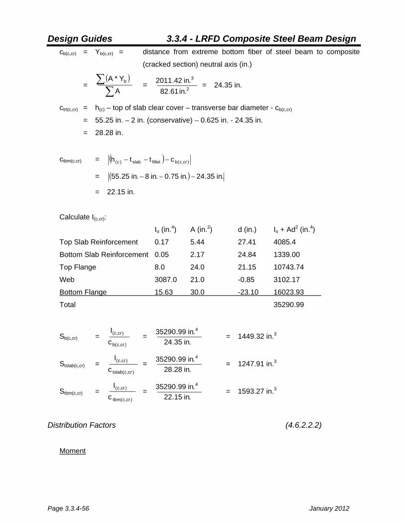
Design Guides 3.3.4 - LRFD Composite Steel Beam Design
Page 3.3.4-56 January 2012
cb(c,cr) = Yb(c,cr) = distance from extreme bottom fiber of steel beam to composite
(cracked section) neutral axis (in.)
= ( )∑
∑A
Y*A b = 2
3
.in61.82.in42.2011 = 24.35 in.
ctrt(c,cr) = h(c) – top of slab clear cover – transverse bar diameter - cb(c,cr)
= 55.25 in. – 2 in. (conservative) – 0.625 in. - 24.35 in.
= 28.28 in.
ctbm(c,cr) = ( ) )cr,c(bfilletslab)c( ctth −−−
= ( ) .in35.24.in75.0.in8.in25.55 −−−
= 22.15 in.
Calculate I(c,cr):
Io (in.4) A (in.2) d (in.) Io + Ad2 (in.4)
Top Slab Reinforcement 0.17 5.44 27.41 4085.4
Bottom Slab Reinforcement 0.05 2.17 24.84 1339.00
Top Flange 8.0 24.0 21.15 10743.74
Web 3087.0 21.0 -0.85 3102.17
Bottom Flange 15.63 30.0 -23.10 16023.93
Total 35290.99
Sb(c,cr) = )cr,c(b
)cr,c(
cI
= .in35.24.in99.35290 4
= 1449.32 in.3
Stslab(c,cr) = )cr,c(tslab
)cr,c(
cI
= .in28.28.in99.35290 4
= 1247.91 in.3
Stbm(c,cr) = )cr,c(tbm
)cr,c(
cI
= .in15.22.in99.35290 4
= 1593.27 in.3
Distribution Factors (4.6.2.2.2)
Moment

Design Guides 3.3.4 - LRFD Composite Steel Beam Design
January 2012 Page 3.3.4-57
g1 = 1.0
3s
g3.04.0
Lt0.12
KLS
0.14S06.0 ⎟
⎟⎠
⎞⎜⎜⎝
⎛⎟⎠⎞
⎜⎝⎛
⎟⎠⎞
⎜⎝⎛+ (Table 4.6.2.2.2b-1)
Where:
S = 7.25 ft.
L = 98.75 ft. 1.0
3s
g
Lt0.12K
⎟⎟⎠
⎞⎜⎜⎝
⎛ = 1.02 (Table 4.6.2.2.1-2)
g1 = ( )02.1.ft75.98
.ft25.70.14
.ft25.706.03.04.0
⎟⎟⎠
⎞⎜⎜⎝
⎛⎟⎠⎞
⎜⎝⎛+
= 0.418
The distribution factor for multiple-lanes loaded, gm, is calculated as:
gm = 1.0
3s
g2.06.0
Lt0.12
KLS
5.9S075.0 ⎟
⎟⎠
⎞⎜⎜⎝
⎛⎟⎠⎞
⎜⎝⎛
⎟⎠⎞
⎜⎝⎛+ (Table 4.6.2.2.2b-1)
= ( )02.1.ft75.98
.ft25.75.9
.ft25.7075.02.06.0
⎟⎟⎠
⎞⎜⎜⎝
⎛⎟⎠⎞
⎜⎝⎛+
= 0.589
The distribution factor for multiple-lanes loaded controls.
Moment (fatigue loading)
g1 (fatigue) = mg1 =
2.1418.0 = 0.348
Shear and Reaction
g1 = 0.25
S36.0 + = 0.25
.ft25.736.0 + (Table 4.6.2.2.3a-1)
= 0.650
gm = 0.2
35S
12S2.0 ⎟
⎠⎞
⎜⎝⎛−⎟
⎠⎞
⎜⎝⎛+ =
0.2
35.ft25.7
12.ft25.72.0 ⎟
⎠⎞
⎜⎝⎛−⎟
⎠⎞
⎜⎝⎛+ (Table 4.6.2.2.3a-1)
= 0.761

Design Guides 3.3.4 - LRFD Composite Steel Beam Design
Page 3.3.4-58 January 2012
The distribution factor for multiple-lanes loaded controls.
Skew correction = ( )θ⎟⎟⎠
⎞⎜⎜⎝
⎛+ tan
KLt0.12
2.013.0
g
3s
= ( ) ( )o20tan97.02.01+
= 1.07
Note that the term 3.0
g
3s
KLt0.12
⎟⎟⎠
⎞⎜⎜⎝
⎛is taken as 0.97. This is found in Table 4.6.2.2.1-2.
Deflection
g (deflection) = ⎟⎟⎠
⎞⎜⎜⎝
⎛
b
L
NN
m = ⎟⎠⎞
⎜⎝⎛
6385.0 = 0.425
Dead Loads
Positive Moment Region
DC1:
Beam:
( )( ) ( )( ) ( )( )[ ] ( )15.1.in144
.ft1.in875.0.in12.in4375.0.in42.in75.0.in12ftk49.0 2
2
3 ⎟⎟⎠
⎞⎜⎜⎝
⎛++⎟
⎠⎞
⎜⎝⎛
= 0.148 k/ft.
Slab: ( ) ( ).ft25.7.ft/.in12
in8.ft/k15.0 3⎟⎟⎠
⎞⎜⎜⎝
⎛ = 0.725 k/ft.
Fillet: ( ) ⎟⎟⎠
⎞⎜⎜⎝
⎛⎟⎟⎠
⎞⎜⎜⎝
⎛.ft/.in12
.in12.ft/.in12.in75.0.ft/k15.0 3 = 0.009 k/ft.
Total: = 0.882 k/ft.
Composite
DC2:
Parapets: ( )( )beams6
parapets2.ft/k45.0 = 0.150 k/ft.

Design Guides 3.3.4 - LRFD Composite Steel Beam Design
January 2012 Page 3.3.4-59
DW:
FWS: ( )( ).ft25.7.ft/k050.0 2 = 0.363 k/ft.
Negative Moment Region
DC1:
Beam: ( )( ) ( )( ) ( )( )[ ] ( )15.1.in144
.ft1.in5.2.in12.in5.0.in42.in0.2.in12ftk49.0 2
2
3 ⎟⎟⎠
⎞⎜⎜⎝
⎛++⎟
⎠⎞
⎜⎝⎛
= 0.293 k/ft.
Slab: ( ) ( ).ft25.7.ft/.in12
in8.ft/k15.0 3⎟⎟⎠
⎞⎜⎜⎝
⎛ = 0.725 k/ft.
Fillet: ( ) ⎟⎟⎠
⎞⎜⎜⎝
⎛⎟⎟⎠
⎞⎜⎜⎝
⎛.ft/.in12
.in12.ft/.in12.in75.0.ft/k15.0 3 = 0.009 k/ft.
Total: = 1.027 k/ft.
Composite
DC2:
Parapets: ( )( )beams6
parapets2.ft/k45.0 = 0.150 k/ft.
DW:
FWS: ( )( ).ft25.7.ft/k050.0 2 = 0.363 k/ft.
Positive Moment Region: Calculate Moments and Shears
Using the bridge and section data shown above, the following moments and shears have
been calculated:
At point 0.375L in span 1 (near the point of maximum positive moment) and 0.625L in span 2,
the unfactored distributed moments are:
MDC1 = 485.3 k-ft.
MDC2 = 86.8 k-ft.
MDW = 209.8 k-ft.

Design Guides 3.3.4 - LRFD Composite Steel Beam Design
Page 3.3.4-60 January 2012
MLL+IM = 1213.9 k-ft.
The maximum unfactored construction loading occurs near point 0.35L in span 1 and 0.65L
in span 2:
CONSTDCM = 517.0 k-ft.
CONSTIMLLM + = 106.1 k-ft.
As per Bridge Manual 3.3.22, a diaphragm (diaphragm location 3) has been placed at the
point of maximum Strength I moment. The maximum construction loading occurs between
this diaphragm and diaphragm that precedes it. The corresponding construction loading
factored moments for the diaphragm locations (brace points) and midpoint for these
diaphragms are:
1POINTBRACE
ISTRENGTHM = 752.4 k-ft., corresponding to diaphragm location 2
MIDPOINTISTRENGTHM = 824.7 k-ft., corresponding to the midpoint of diaphragm locations 2 and
3 2POINTBRACE
ISTRENGTHM = 823.0 k-ft., corresponding to diaphragm location 3
For this bridge, the maximum factored Fatigue loading range occurs near point 0.53L in span
1 and 0.47L in span 2. For simplicity, assume that a diaphragm connection point and shear
stud weldment are present at this location. This is conservative and will allow us to check all
detail categories using one fatigue range, as opposed to calculating multiple fatigue ranges
for different aspects of design.
+IFATIGUEM = 535.5 k-ft. −
IFATIGUEM = -235.2 k-ft.
+IIFATIGUEM = 267.8 k-ft. −
IIFATIGUEM = -117.6 k-ft.
These values contain impact and include γ of 1.5 for Fatigue I and 0.75 for Fatigue II.

Design Guides 3.3.4 - LRFD Composite Steel Beam Design
January 2012 Page 3.3.4-61
The factored, distributed moments for Strength Limit State, Service Limit State, and
Constructibility Limit State are found to be:
MSTRENGTH I = 3154.2 k-ft.
MSERVICE II = 2360.0 k-ft.
CONSTISTRENGTHM = 831.9 k-ft.
The maximum factored shears for the positive moment section have been found to be:
VCONST = 49.9 kips (@ abutment)
VSTRENGTH I = 219.8 kips (@ abutment)
Positive Moment Region: Check Cross-Section Proportion Limits (6.10.2)
Check Web Proportions
150tDw
≤ (Eq. 6.10.2.1.1-1)
wtD =
.in4375.0.in42 = 96 ≤ 150 O.K.
Check Flange Proportions
i) 0.12t2
b
f
f ≤ (Eq. 6.10.2.2-1)
tf
tf
t2b
= .)in75.0(2
.in12 = 8 bf
bf
t2b
= .)in875.0(2
.in12 = 6.86
8 and 6.86 < 12.0 O.K.
ii) 6Dbf ≥ (Eq. 6.10.2.2-1)
bf = 12 in.
6D =
6.in42 = 7 in.
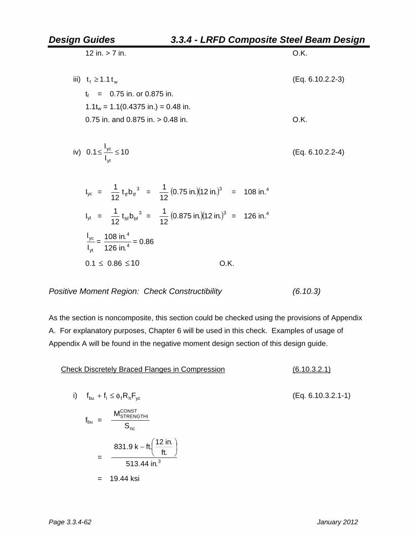
Design Guides 3.3.4 - LRFD Composite Steel Beam Design
Page 3.3.4-62 January 2012
12 in. > 7 in. O.K.
iii) wf t1.1t ≥ (Eq. 6.10.2.2-3)
tf = 0.75 in. or 0.875 in.
1.1tw = 1.1(0.4375 in.) = 0.48 in.
0.75 in. and 0.875 in. > 0.48 in. O.K.
iv) 10II
1.0yt
yc ≤≤ (Eq. 6.10.2.2-4)
Iyc = 3tftfbt
121
= ( )( )3.in12.in75.0
121 = 108 in.4
Iyt = 3bfbfbt
121
= ( )( )3.in12.in875.0
121 = 126 in.4
yt
yc
II
= 4
4
.in126
.in108= 0.86
0.1 ≤ 0.86 10≤ O.K.
Positive Moment Region: Check Constructibility (6.10.3)
As the section is noncomposite, this section could be checked using the provisions of Appendix
A. For explanatory purposes, Chapter 6 will be used in this check. Examples of usage of
Appendix A will be found in the negative moment design section of this design guide.
Check Discretely Braced Flanges in Compression (6.10.3.2.1)
i) ychflbu FRff φ≤+ (Eq. 6.10.3.2.1-1)
fbu = nc
CONSTISTRENGTH
SM
= 3.in44.513
.ft.in12.ftk9.831 ⎟⎠
⎞⎜⎝
⎛−
= 19.44 ksi

Design Guides 3.3.4 - LRFD Composite Steel Beam Design
January 2012 Page 3.3.4-63
fl = assume 0 ksi
φf = 1.00 (6.5.4.2)
Rh = 1.0 (6.10.1.10.1)
Fyc = 50 ksi
fbu + fl = 19.44 ksi < (1.00)(1.0)(50 ksi) = 50 ksi O.K.
ii) ( )ncflbu Ff31f φ≤+ (Eq. 6.10.3.2.1-2)
Fnc is taken as the lesser Fnc(FLB) and Fnc(LTB) (6.10.8.2.1)
Determine Fnc(FLB): (6.10.8.2.2)
λf =fc
fc
t2b
= ( ).in75.02.in0.12 = 8 (Eq. 6.10.8.2.2-3)
λpf =ycFE38.0 =
ksi50ksi2900038.0 = 9.2 (Eq. 6.10.8.2.2-5)
λf ≤ λpf, therefore:
Fnc(FLB) = RbRhFyc (Eq. 6.10.8.2.2-1)
Where:
Rb = 1.0 (Eq. 6.10.1.10.2)
Rh = 1.0 (Eq. 6.10.1.10.1)
Fyc = 50 ksi
Fnc(FLB) = (1.0)(1.0)(50 ksi) = 50 ksi
Determine Fnc(LTB):
Lb = ( ) ⎟⎠
⎞⎜⎝
⎛−.ft
.in12.ft96.22.ft37 = 168.5 in. (6.10.8.2.3)
Lp = yc
t FEr0.1 (Eq. 6.10.8.2.3-4)
Where:

Design Guides 3.3.4 - LRFD Composite Steel Beam Design
Page 3.3.4-64 January 2012
rt =
⎟⎟⎠
⎞⎜⎜⎝
⎛+
fcfc
wc
fc
tbtD
31112
b (Eq. 6.10.8.2.3-9)
Where:
Dc = ct(nc) – ttf
= 22.62 in. – 0.75 in.
= 21.87 in.
rt =
⎟⎟⎠
⎞⎜⎜⎝
⎛+
.)in75.0.)(in0.12(.)in4375.0.)(in87.21(
31112
.in12
= 2.98 in.
Lp = ksi50
ksi29000.)in98.2(0.1 = 71.77 in.
Lr = yr
t FErπ (Eq. 6.10.8.2.3-5)
Where:
Fyr = lesser of Fyw and 0.7Fyc but not less than 0.5Fyc
= 0.7(50 ksi)
= 35 ksi
Lr = ksi35
ksi29000.)in98.2(π
= 269.5 in.
Lp < Lb < Lr, therefore:
Fnc(LTB) = ychbychbpr
pb
ych
yrb FRRFRR
LLLL
FRF
11C ≤⎥⎥⎦
⎤
⎢⎢⎣
⎡⎟⎟⎠
⎞⎜⎜⎝
⎛
−−
⎟⎟⎠
⎞⎜⎜⎝
⎛−−
(Eq. 6.10.8.2.3-2)

Design Guides 3.3.4 - LRFD Composite Steel Beam Design
January 2012 Page 3.3.4-65
Where:
Fyr = 35 ksi
Rh = 1.0
Fyc = 50 ksi
Lb = 168.5 in.
Lp = 71.77 in.
Lr = 269.5 in.
For 2
mid
ff
> 1, or f2 = 0, Cb = 1.0 (Eq. 6.10.8.2.3-6)
As there are no composite loads and no change in section over the braced
length, 2
mid
ff
= 2
mid
MM
. As Mmid is greater than both moments at bracepoints
(824.7 k-ft. vs. 823.0 k-ft. and 752.4 k-ft.), 2
mid
MM
>1 and Cb = 1.0.
Rb = 1.0
Fnc(LTB) = ( ) ( ) ( ) ( ) ( ) ( )ksi500.10.1.in77.71.in5.269.in77.71.in5.168
ksi500.1ksi35110.1 ⎥
⎦
⎤⎢⎣
⎡⎟⎟⎠
⎞⎜⎜⎝
⎛−−
⎟⎟⎠
⎞⎜⎜⎝
⎛−−
= 42.66 ksi
RbRhFyc = (1.0)(1.0)(50 ksi) = 50 ksi
Fnc(LTB) = 42.66 ksi
Fnc = 42.66 ksi
lbu f31f + = )ksi0(
31ksi44.19 + = 19.44 ksi
φfFnc = 1.00(42.66 ksi) = 42.66 ksi
19.44 ksi < 42.66 ksi O.K.

Design Guides 3.3.4 - LRFD Composite Steel Beam Design
Page 3.3.4-66 January 2012
iii) fbu ≤ φfFcrw (Eq. 6.10.3.2.1-3)
Equation 6.10.3.2.1-3 need not be checked for non-slender webs. Check slenderness:
w
c
tD2
< ycFE7.5 (Eq. 6.10.6.2.3-1)
w
c
tD2
= ( ).in4375.0.in87.212 = 99.98
ycFE7.5 =
ksi50ksi290007.5 = 137.27
99.98 < 137.27, the section is not slender and Eq. 6.10.3.2.1-3 need not be checked.
Check Discretely Braced Flanges in Tension (6.10.3.2.2)
ythflbu FRff φ≤+ (Eq. 6.10.3.2.2-1)
fbu = nc
CONSTISTRENGTH
SM
= 3.in66.552
.ft.in12.ftk9.831 ⎟⎠
⎞⎜⎝
⎛− = 18.06 ksi
18.06 ksi + 0 ksi = 18.06 ksi < (1.00)(1.0)(50 ksi) = 50 ksi O.K.
Check Shear (6.10.3.3)
As VCONST = 49.9 k < VSTRENGTH I = 219.8 k, and both loads are applied to the same web
section, construction shear loading will not control the design by inspection.
Positive Moment Region: Check Service Limit State (6.10.4)
Check Permanent Deformations (6.10.4.2)
The top steel flange shall satisfy:
i) ( ) ( )yfhf FR95.0f ≤ (Eq. 6.10.4.2.2-1)

Design Guides 3.3.4 - LRFD Composite Steel Beam Design
January 2012 Page 3.3.4-67
Where:
ff =( )
9n
IMLL
27n
DW2DC
nc
1DC
SM3.1
SMM
SM
=
+
=+
++ (Eq. D6.2.2-1)
Where:
MDC1 = 485.3 k-ft.
MDC2 = 86.8 k-ft.
MDW = 209.8 k-ft.
MLL+IM = 1213.9 k-ft.
Sn=9 = 7309.82 in.3
Sn=27 = 2013.21 in.3
Snc = 513.44 in.3
ff =( ) ( )
333 .in82.7309.ft
.in12.ftk9.12133.1
.in21.2013.ft
.in12.ftk 8.2098.86
.in44.513.ft
.in12.ftk3.485 ⎟⎠⎞
⎜⎝⎛−
+⎟⎠⎞
⎜⎝⎛−+
+⎟⎠⎞
⎜⎝⎛−
= 15.7 ksi < (0.95)(1.0)(50.0 ksi) = 47.5 ksi O.K.
The bottom flange shall satisfy:
ii) ( ) ( )yfhl
f FR95.02ff ≤+ (Eq. 6.10.4.2.2-2)
Where:
fl = 0 ksi for skews less than 45 degrees
ff = ( )
9n
IMLL
27n
DW2DC
nc
1DC
SM3.1
SMM
SM
=
+
=+
++ (Eq. D6.2.2-1)
Where:
MDC1 = 485.3 k-ft.
MDC2 = 86.8 k-ft.
MDW = 209.8 k-ft.
MLL+IM = 1213.9 k-ft.
Sn=9 = 788.90 in.3

Design Guides 3.3.4 - LRFD Composite Steel Beam Design
Page 3.3.4-68 January 2012
Sn=27 = 723.98 in.3
Snc = 552.66 in.3
ff =( ) ( )
333 .in90.788.ft
.in12.ftk9.12133.1
.in98.723.ft
.in12.ftk 8.2098.86
.in66.552.ft
.in12.ftk3.485 ⎟⎠⎞
⎜⎝⎛−
+⎟⎠⎞
⎜⎝⎛−+
+⎟⎠⎞
⎜⎝⎛−
= 39.46 ksi
ff + 2fl = 39.46 ksi + 0 ksi = 39.46 ksi
(0.95)(1.0)(50.0 ksi) = 47.5 ksi > 39.46 ksi O.K.
As this is a composite section in positive flexure and D / tw < 150, Eq. 6.10.4.2.2-4 need
not be checked.
Positive Moment Region: Check Fatigue and Fracture Limit State (6.10.5)
Determine (ADTT)SL and Appropriate Limit State
(ADTT)75, SL = p(ADTT) (Eq. 3.6.1.4.2-1)
Where:
ADTT = ( )5.0day
trucks300years20years57
daytrucks300
daytrucks600 ⎟⎟
⎠
⎞⎜⎜⎝
⎛+⎟⎟
⎠
⎞⎜⎜⎝
⎛⎟⎟⎠
⎞⎜⎜⎝
⎛−
= 713 trucks/day
p = 1.0 for one lane (not counting shoulders) (Table 3.6.1.4.2-1)
(ADTT)SL = 1.0(713 trucks/day) = 713 trucks/day
From Table 6.6.1.2.3-1, use Detail Category A for base metal checks in bottom flange at
maximum fatigue range, use Detail Category C for base metal checks in top flange at
maximum fatigue range, and use Detail Category C’ for base metal checks at brace
points. From Table 6.6.1.2.3-2, the 75-year infinite life equivalent (ADTT)SL is 530
trucks/day for Category A, 1290 trucks/day for Category C, and 745 trucks/day for

Design Guides 3.3.4 - LRFD Composite Steel Beam Design
January 2012 Page 3.3.4-69
Category C’. Therefore, use Fatigue I (infinite life) limit state for Category A checks, and
Fatigue II (finite life) limit state for Category C and C’ checks.
Determine Stress Range and Compare to Allowable Stress Range
( ) ( )nFf Δ≤Δγ (Eq. 6.6.1.2.2-1)
( )fΔγ = 9n
FATIGUEFATIGUE
SMM
=
−+ − + fl
Where:
+IFATIGUEM = 535.5 k-ft. −
IFATIGUEM = -235.2 k-ft.
+IIFATIGUEM = 267.8 k-ft. −
IIFATIGUEM = -117.6 k-ft.
Sn=9 = 788.90 in.3 for outside of bottom flange
= 7309.82 in.3 for outside of top flange
= 806.82 in.3 for inside of bottom flange
γfl = = 0 ksi
( )fΔγ = ( )
3.in90.788.ft
.in12.ftk )2.235(5.535 ⎟⎠⎞
⎜⎝⎛−−−
= 11.72 ksi for outside of bottom flange
( )fΔγ = ( )
3.in82.806.ft
.in12.ftk )6.117(8.267 ⎟⎠⎞
⎜⎝⎛−−−
= 5.73 ksi for inside of bottom flange
( )fΔγ = ( )
3.in82.7309.ft
.in12.ftk )6.117(8.267 ⎟⎠⎞
⎜⎝⎛−−−
= 0.63 ksi for top of top flange
For Fatigue I Limit State:
( )nFΔ = ( )THFΔ (Eq. 6.6.1.2.5-1)

Design Guides 3.3.4 - LRFD Composite Steel Beam Design
Page 3.3.4-70 January 2012
(ΔF)TH = 24.0 ksi for Category A.
( )fΔγ = 11.72 ksi < 24.0 ksi O.K.
For Fatigue II Limit State:
( )nFΔ = 31
NA⎟⎠⎞
⎜⎝⎛ (Eq. 6.6.1.2.5-2)
Where:
A = 44 × 108 ksi for Detail Category C and C’
N = ( ) ⎟⎟⎠
⎞⎜⎜⎝
⎛⎟⎠⎞
⎜⎝⎛
⎟⎟⎠
⎞⎜⎜⎝
⎛day
trucks)ADTT(truckcyclesnyears75
yeardays365 SL,5.37
(Eq. 6.6.1.2.5-3)
n = 1.0 (Table 6.6.1.2.5-2)
(ADTT)37.5, SL = ( )5.0day
trucks300years20years5.37
daytrucks300
daytrucks600 ⎟⎟
⎠
⎞⎜⎜⎝
⎛+⎟⎟
⎠
⎞⎜⎜⎝
⎛⎟⎟⎠
⎞⎜⎜⎝
⎛−
= 431 trucks/day
N = ( ) ⎟⎟⎠
⎞⎜⎜⎝
⎛⎟⎠⎞
⎜⎝⎛
⎟⎟⎠
⎞⎜⎜⎝
⎛daytrucks431
truckcycle1years75
yeardays365
= 11.8 × 10⁶ cycles
( )nFΔ = 31
6
8
cycles108.11cycles1044
⎟⎟⎠
⎞⎜⎜⎝
⎛
×× = 7.20 ksi
( )fΔγ = 5.73 ksi and 0.63 ksi < 7.20 ksi O.K.
Positive Moment Region: Check Strength Limit State (Moment) (6.10.6)
Check Composite Sections in Positive Flexure (6.10.6.2.2)
Check Compactness
i) The bridge is straight or equivalently straight as per 4.6.1.2.4b

Design Guides 3.3.4 - LRFD Composite Steel Beam Design
January 2012 Page 3.3.4-71
ii) Fy = 50 ksi ≤ 70 ksi O.K.
iii) Cross-section proportion limit web requirements are satisfied (see above)
iv) ( )
ycw
cp
FE76.3
tD2
≤ (Eq. 6.10.6.2.2-1)
Find Dp, the depth to the plastic neutral axis from the top of the slab, to determine
Dcp, the depth of the web in compression at the plastic moment capacity.
Per Table D6.1-1:
Prt = force in top reinforcement in fully plastic section (k)
= FyrtArt = 60 ksi(2.25 in.2) = 135 k
Ps = force in slab in fully plastic section (k)
= 0.85f’c(eff. flange width)tslab = 0.85(3.5 ksi)(87 in.)(8 in.) = 2070.6 k
Prb = force in bottom reinforcement in fully plastic section (k)
= FyrbArt = 60 ksi(2.17 in.2) = 130.2 k
Pc = force in top flange in fully plastic section (k)
= Fycbfctfc = (50 ksi)(12 in.)(0.75 in.) = 450 k
Pw = force in web in fully plastic section (k)
= FywDtw = (50 ksi)(42 in.)(0.4375 in.) = 918.75 k
Pt = force in bottom flange in fully plastic section (k)
= Fytbfttft = (50 ksi)(12 in.)(0.875 in.) = 525 kips
The fully plastic force in the steel beam is:
Pt + Pw + Pc = 450 k + 918.75 k + 525.0 k = 1893.75 k
The fully plastic (ultimate) force in the slab is:
rtrbs PPP ++ = 2070.6 k + 130.2 k + 135.0 k = 2335.8 kips
Pt + Pw + Pc < rtrbs PPP ++
∴The plastic neutral axis is in the slab, take Dcp as 0. However, as Dp and Y are useful in later calculations, they should still be calculated.

Design Guides 3.3.4 - LRFD Composite Steel Beam Design
Page 3.3.4-72 January 2012
Check Case III:
rtrbss
rb PPPtc
++⎟⎟⎠
⎞⎜⎜⎝
⎛ =
( ) ( ) k0.135k2.130k6.2070.in8
.in625.05.1.in1.in8 ++⎟⎟⎠
⎞⎜⎜⎝
⎛ −−
= 1834.33 k
Pt + Pw + Pc = 525 k + 918.75 k + 450 k
= 1893.75 k
Pt + Pw + Pc > rtrbss
rb PPPtc
++⎟⎟⎠
⎞⎜⎜⎝
⎛,∴ Y = ⎟⎟
⎠
⎞⎜⎜⎝
⎛ −−++
s
rbrttwcs P
PPPPPt
Y = ( ) ⎟⎟⎠
⎞⎜⎜⎝
⎛ −−++k6.2070
k2.130k135k525k75.918k450.in8
= 6.29 in., measured from top of slab. Therefore Dp = Y = 6.29 in.
( )w
cp
tD2
= ( )
.in4375.002
= 0.0
ycFE76.3 =
ksi50ksi2900076.3 = 90.55
0 < 90.55 O.K.
The section is compact.
Check Flexural Resistance (6.10.7)
( ) ( ) ( )nfxtlu MSf31M φ≤+ (Eq. 6.10.7.1.1-1)
MSTRENGTH I = 1.25(485.3 k-ft.+86.8 k-ft.)+1.5(209.8 k-ft.) + 1.75(1213.9 k-ft.)

Design Guides 3.3.4 - LRFD Composite Steel Beam Design
January 2012 Page 3.3.4-73
= 3154.2 k-ft.
fl = 0 ksi
Sxt = yt
yt
FM
Myt = DW2DC1DC)n3,c(b
DW
)n3,c(b
2DC
)nc(b
1DCyf)n,c(b M75.1M5.1M25.1
SM5.1
SM25.1
SM25.1
FS +++⎟⎟⎠
⎞⎜⎜⎝
⎛−−−
(Eqs. D6.2.2-1,2)
= ( ) ( ) ( ) ( )⎟⎟⎠
⎞⎜⎜⎝
⎛⎟⎟⎠
⎞⎜⎜⎝
⎛ −+−+−⎟⎠⎞
⎜⎝⎛− 333
3
.in98.723.ftk8.2095.1
.in98.723.ftk8.8625.1
.in66.552.ftk3.48525.1
.ft.in12ksi50.in9.788
+ ⎟⎠⎞
⎜⎝⎛
.ft.in12 ( )ft.)-k 1.5(209.8 + ft.)-k 1.25(86.8 + ft.)-k 1.25(485.3
= 35878 k-in.
Sxt = ksi50
.ink35878 −
= 717.6 in.3
For Dp ≤ 0.1Dt, Mn = Mp (Eq. 6.10.7.1.2-1)
Otherwise, Mn =⎥⎥⎦
⎤
⎢⎢⎣
⎡⎟⎟⎠
⎞⎜⎜⎝
⎛−
t
pp D
D7.007.1M (Eq. 6.10.7.1.2-2)
Dp = 6.29 in.
0.1Dt = 0.1(0.875 in. + 42 in. + 0.75 in. + 0.75 in. + 8 in.) = 5.24 in. < 6.29 in.
∴Mn =⎥⎥⎦
⎤
⎢⎢⎣
⎡⎟⎟⎠
⎞⎜⎜⎝
⎛−
t
pp D
D7.007.1M (Eq. 6.10.7.1.2-2)
Where:
As per Table D6.1-1, Mp for Case III is calculated as follows:
Mp = [ ]ttwwccrbrbrtrts
s2
dPdPdPdPdPt2PY
+++++⎟⎟
⎠
⎞
⎜⎜
⎝
⎛
Where:
Y = 6.29 in.
drt = distance from plastic neutral axis to centroid of top reinforcement (in.)

Design Guides 3.3.4 - LRFD Composite Steel Beam Design
Page 3.3.4-74 January 2012
= 6.29 in. – 2.5 in. – 1.5(0.625 in.) = 2.85 in.
drb = distance from plastic neutral axis to centroid of bottom reinforcement
(in.)
= 6.29 in. – (8 in. – 1 in. – 1.5(0.625 in.) = 0.23 in.
dc = distance from plastic neutral axis to centroid of top flange (in.)
= (8 in. – 6.29 in.) + 0.75 + 0.5(0.75 in.) = 2.84 in.
dw = distance from plastic neutral axis to centroid of web (in.)
= (8 in. – 6.29 in.) + 0.75 in. + 0.75 in. + 0.5(42 in.) = 24.21 in.
dt = distance from plastic neutral axis to centroid of tension flange (in.)
= (8 in. – 6.29 in.) + 0.75 in. + 0.75 in. + 42 in. + 0.5(0.875 in.) = 45.65 in.
Mp = .)in8(2
)k6.2070(.)in29.6( 2
+ (135 k)(2.85 in.) + (130.2 k)(0.23 in.) +
(450 k)(2.84 in.) + .)in65.45)(k525(.)in21.24)(k75.918( +
= 53021.97 k-in.
Mn = ( ) ⎥⎦
⎤⎢⎣
⎡⎟⎟⎠
⎞⎜⎜⎝
⎛−−
.in38.52.in29.67.007.1.ink97.53021
= 52276.54 k-in.
φfMn = 1.00(52276.54 k-in.) = 52276.54 k-in.
( ) ( )xtlu Sf31M + = 3154.2 k-ft. ⎟
⎠⎞
⎜⎝⎛
.ft.in12 + ( ) ( )3.in6.717ksi0
31
= 37850.4 k-in. < 52276.54 k-in. O.K.
Check Eq. 6.10.7.1.2-3:
Mn ≤ 1.3RhMy (Eq. 6.10.7.1.2-3)
Where:
Rh = 1.0
My = 35878 k-in.

Design Guides 3.3.4 - LRFD Composite Steel Beam Design
January 2012 Page 3.3.4-75
1.3RhMy = 46641 k-in. < 52276.54 k-in.
Recalculate Mn using 46641 k-in.
Mn = ( ) ⎥⎦
⎤⎢⎣
⎡⎟⎟⎠
⎞⎜⎜⎝
⎛−−
.in38.52.in29.67.007.1.ink46641
= 45985 k-in.
( ) ( )xtlu Sf31M + = 37850.4 k-in. < 45985 k-in. O.K.
Check Ductility Requirement (6.10.7.3)
Dp ≤ 0.42Dt (Eq. 6.10.7.3-1)
Where:
Dp = 6.29 in.
0.42Dt = 0.42(52.38 in.) = 22.0 in.
6.29 in. < 22.0 in. O.K.
Positive Moment Region: Check Strength Limit State (Shear) (6.10.9)
The maximum shear for the positive moment section occurs at the abutments. The end section
of the beam technically could be considered stiffened because the first diaphragm is close
enough to the bearing stiffener to warrant it. However, this is irrelevant because end sections of
stiffened webs and unstiffened webs use the same equations for shear capacity of their
respective webs:
Vu ≤ φvVn (Eq. 6.10.9.1-1)
Where:
φv = 1.00 (6.5.4.2)
Vu = 219.2 kips
Vn = Vcr = CVp (Eq. 6.10.9.2-1)

Design Guides 3.3.4 - LRFD Composite Steel Beam Design
Page 3.3.4-76 January 2012
Where:
wtD
= 96
ywFEk12.1 =
)ksi50()5)(ksi29000(12.1 = 60.3
ywFEk40.1 =
)ksi50()5)(ksi29000(40.1 = 75.4
∴ C = ⎟⎟⎠
⎞⎜⎜⎝
⎛
⎟⎟⎠
⎞⎜⎜⎝
⎛ yw2
w
FEk
tD
57.1 (Eq. 6.10.9.3.2-6)
= ( )( )⎟⎟⎠
⎞⎜⎜⎝
⎛
⎟⎟⎠
⎞⎜⎜⎝
⎛ ksi505ksi29000
.in4375.0.in42
57.12
= 0.49
Vp = 0.58FywDtw (Eq. 6.10.9.2-2)
= 0.58(50 ksi)(42 in.)(0.4375 in.)
= 532.9 k
CVp = 0.49(532.9 k) = 261.1 k
219.2 kips < 261.1 kips O.K.
The proposed positive moment section is adequate.
Negative Moment Region: Calculate Moments and Shears
The regions adjacent to the pier control the negative moment design of the beams. The first
unstiffened web section controls the shear design of the beams.

Design Guides 3.3.4 - LRFD Composite Steel Beam Design
January 2012 Page 3.3.4-77
Since an unstiffened web design is already shown in the positive moment region, in order to
illustrate a stiffened web design the regions closest to the pier will be shown for shear design
even though they do not control the final design of the beam.
At the pier, the unfactored distributed moments are:
MDC1 = -1466.9 k-ft.
MDC2 = -225.6 k-ft.
MDW = -545.2 k-ft.
MLL+IM = -1669.0 k-ft.
The maximum construction loading moments are found at the pier:
CONSTDCM = -1543.5 k-ft.
CONSTIMLLM + = -307.9 k-ft.
The corresponding construction loading factored moments for the diaphragm locations
(brace points) and midpoint for these diaphragms are:
1POINTBRACE
ISTRENGTHM = -2468.2 k-ft., corresponding to the pier
MIDPOINTISTRENGTHM = -2238.8 k-ft., corresponding to the first midpoint in the second span
2POINTBRACEISTRENGTHM = -2017.8 k-ft., corresponding to the first diaphragm in the second span
Note that the last diaphragm section in the first span has a larger unbraced length, but
smaller moments. In a full design this bay would also need to be checked. However, for
brevity, only the pier section will be checked in this design guide.
The moments resulting in the maximum fatigue stress range occur near the point of splice:
+IFATIGUEM = 400.9 k-ft. −
IFATIGUEM = -301.6 k-ft.
+IIFATIGUEM = 200.5 k-ft. −
IIFATIGUEM = -150.8 k-ft.

Design Guides 3.3.4 - LRFD Composite Steel Beam Design
Page 3.3.4-78 January 2012
These values contain impact and include γ of 1.5 for Fatigue I and 0.75 for Fatigue II.
The factored, distributed moments for Strength Limit State, Service Limit State, and
Constructibility Limit State are found to be:
MSTRENGTH I = -5854.1 k-ft.
MSERVICE II = -4407.3 k-ft.
CONSTISTRENGTHM = -2468.2 k-ft.
The factored shears at the pier have been found to be:
VCONST = 103.9 kips (@ pier)
VSTRENGTH I = 300.5 kips (@ pier)
Note, again, that the pier section is being used even though it does not control the shear
design. This is to illustrate a stiffened web design.
Negative Moment Region: Check Cross-Section Proportion Limits (6.10.2)
Check Web Proportions
150tD
w≤ (Eq. 6.10.2.1.1-1)
wtD =
.in5.0.in42 = 84 ≤ 150 O.K.
Check Flange Proportions
i) 0.12t2
b
f
f ≤ (Eq. 6.10.2.2-1)
tf
tf
t2b
= .)in2(2.in12 = 3
bf
bf
t2b
= )5.2(2.in12
= 2.4

Design Guides 3.3.4 - LRFD Composite Steel Beam Design
January 2012 Page 3.3.4-79
3 and 2.4 < 12.0 O.K.
ii) 6Dbf ≥ (Eq. 6.10.2.2-1)
bf = 12 in.
6D =
6.in42 = 7 in.
12 in. > 7 in. O.K.
iii) wf t1.1t ≥ (Eq. 6.10.2.2-3)
tf = 2.0 in. or 2.5 in.
1.1tw = 1.1(0.5 in.) = 0.55 in.
2.0 in. and 2.5 in. > 0.55 in. O.K.
iv) 10II
1.0yt
yc ≤≤ (Eq. 6.10.2.2-4)
Iyc = 3bfbfbt
121
= ( )( )3.in12.in5.2
121 = 360 in.4
Iyt = 3tftfbt
121
= ( )( )3.in12.in0.2
121 = 288 in.4
yt
yc
II
= 4
4
.in288
.in360= 1.25
0.1 ≤ 1.25 10≤ O.K.
Negative Moment Region: Check Constructibility (6.10.3, App. A6)
Check Applicability of Appendix A6 (A6.1.1)
The bridge is straight, Fy for all portions of the girder is 70 ksi or less, and yt
yc
II
> 0.3. The
skew is 20 degrees and there are no curvature effects.

Design Guides 3.3.4 - LRFD Composite Steel Beam Design
Page 3.3.4-80 January 2012
Verify that beam is non-slender. w
c
tD2
< ycFE7.5 :
For noncomposite sections in negative flexure:
Dc = Yb(nc) – tbf = 21.64 in. – 2.5 in. = 19.14 in.
w
c
tD2
= ( ).in5.0
.in14.192 = 76.6
ycFE7.5 =
ksi50ksi290007.5 = 137.3
76.6 < 137.3. Therefore, Appendix A may be used.
Determine Web Plastification Factors (App A6.2)
Check Web Compactness. If w
cp
tD2
≤ λpw(Dcp), the web is compact (Eq. A6.2.1-1).
Dcp = YPNA - tbf
Determine YPNA for noncomposite section:
(50 ksi)(12 in.)(2 in.) + (50 ksi)(0.5 in.)(46.5 in. – YPNA in. – 2 in.) =
(50 ksi)(12 in.)(2.5 in.) + (50 ksi)(0.5 in.)(YPNA in. – 2.5 in.)
YPNA = 17.5 in.
Dcp = 17.5 in. – 2.5 in.
= 15.0 in.
w
cp
tD2
= ( ).in5.0.in0.152 = 60 in.
λpw(Dcp) = 2
yh
p
yc
09.0MR
M54.0
FE
⎟⎟⎠
⎞⎜⎜⎝
⎛−
≤ ⎟⎟⎠
⎞⎜⎜⎝
⎛λ
c
cprw D
D (Eq. A6.2.1-2)
Where:
Rh = 1

Design Guides 3.3.4 - LRFD Composite Steel Beam Design
January 2012 Page 3.3.4-81
Mp = (50 ksi)(12 in.)(2 in.)[42 in. – 15 in. + 0.5(2 in.)] +
(50 ksi)(0.5 in.)(0.5)(42 in. – 15.0 in.)2 +
(50 ksi)(0.5 in.)(0.5)(15.0 in.)2 +
(50 ksi)(12 in.)(2.5 in.)[15.0 in. + 0.5(2.5 in.)]
= 69900 k-in.
My = smaller of Myc and Myt. For noncomposite sections, Myc = FySxc and
Myt = FySxt. By inspection, FySxt is smaller.
= (50 ksi)(1179.37 in.3)
= 58968.50 k-in.
λrw = ycFE7.5 = 137.3, as calculated above.
λpw(Dcp) =
( )( )2
09.0.ink50.589680.1
.ink6990054.0
ksi50ksi29000
⎟⎟⎠
⎞⎜⎜⎝
⎛−
−−
= 79.58
⎟⎟⎠
⎞⎜⎜⎝
⎛λ
c
cprw D
D = ( ) ⎟⎟
⎠
⎞⎜⎜⎝
⎛.in14.19
.in0.153.137 = 107.6 > 79.58, 79.58 controls.
60 < 79.58, therefore Rpc = yc
p
MM
and Rpt = yt
p
MM
Rpc = ( )( )3.in85.1354ksi50.ink69900 − = 1.03 (Eq. A6.2.1-4)
Rpt = ( )( )ksi37.1179ksi50.ink69900 − = 1.19 (Eq. A6.2.1-5)
Check Compression Flange (A6.1.1)
ncfxclu MSf31M φ≤+ (Eq. A6.1.1-1)
Where:
Mu = 2468.2 k-ft.
fl = Assume zero for Constructibility.
Sxc = 1354.85 in.3

Design Guides 3.3.4 - LRFD Composite Steel Beam Design
Page 3.3.4-82 January 2012
φf = 1.00 for flexure (6.5.4.2)
Mnc = smaller of Mnc(FLB) and Mnc(LTB) as calculated in Appendix A6.3
Determine Mnc(FLB):
λf = ( ).in5.22.in12 = 2.4 (Eq. A6.3.2-3)
λpf = ksi50
ksi2900038.0 = 9.15 (Eq. A6.3.2-4)
2.4 < 9.15, ∴Mnc(FLB) = RpcMyc = Mp (Eq. A6.3.2-1)
Mnc(FLB) = 69900 k-in.
Determine Mnc(LTB):
Lb = 54 in. (Eq. A6.3.2-3)
Lp = yc
t FEr0.1 (Eq. A6.3.3-4)
rt =
⎟⎟⎠
⎞⎜⎜⎝
⎛+
fcfc
wc
fc
tbtD
31112
b (Eq. A6.3.3-10)
Dc = Yb - tbf
= 21.64 in. – 2.5 in. = 19.14 in.
rt = ( ) ( )
( ) ( ) ⎟⎟⎠
⎞⎜⎜⎝
⎛+
.in5.2.in12.in5.0.in14.19
31112
.in12
= 3.29 in.
Lp = ( )ksi50
ksi29000.in29.30.1 = 79.23 in.
54 in. < 79.23 in.,
∴Mnc(LTB) = ycpcMR
Where:
Rpc = 1.03 (See FLB computations)
Myc = FySxc = (50 ksi)(1354.85 in.3) = 67742.5 k-in.
Mnc(LTB) = 1.03(67742.5 k-in.)
= 69900 k-in. < 69900 k-in., Mnc(LTB) = Mnc(FLB) = Mp.

Design Guides 3.3.4 - LRFD Composite Steel Beam Design
January 2012 Page 3.3.4-83
Mnc = 69900 k-in.
xclu Sf31M + = ( ) ( )( )3.in9.1354ksi0
31
.ft.in12.ftk2.2468 +⎟⎠
⎞⎜⎝
⎛−
= 29618.4 k-in.
ncfMφ = 1.00(69900 k-in.) = 69900 k-in.
29618.4 k-in. < 69900 k-in. O.K.
Check Tension Flange (A6.4)
Mnt = RptMyt = Mp = 69900 k-in. (Eq. A6.4-1)
29618.4 k-in. < 69900 k-in. O.K.
Check Shear (6.10.3.3)
As VCONST = 103.9 k < VSTRENGTH I = 300.5 k, and the steel web capacity does not change from
construction loading to full Strength I loading, construction shear loading will not control the
web design by inspection.
Negative Moment Region: Check Service Limit State (6.10.4)
Find stresses in slab and compare to 2fr:
ff = ( )
( )( )
( )33 .in15.33979.ft
.in12.ftk0.16693.1
.in0.267627.ft
.in12.ftk 2.5456.225 ⎟⎠⎞
⎜⎝⎛−
+⎟⎠⎞
⎜⎝⎛−+
= 0.98 ksi
2fr = ( ) c'f24.02 = ( ) ( )ksi5.324.02 = 0.90 ksi (6.10.1.7)
0.98 ksi > 0.90 ksi. The deck is assumed to be cracked.
Check Permanent Deformations (6.10.4.2)
i) The top flange shall satisfy ( ) ( )yfhf FR95.0f ≤ (Eq. 6.10.4.2.2-1)

Design Guides 3.3.4 - LRFD Composite Steel Beam Design
Page 3.3.4-84 January 2012
Where:
ff =( )( )33 .in27.1593
.ft.in12.ftk0.16693.1.ftk2.545.ftk6.225
.in37.1179.ft
.in12.ftk9.1466 ⎟⎠⎞
⎜⎝⎛−+−+−
+⎟⎠⎞
⎜⎝⎛−
= 37.07 ksi
Rh = 1.0
Fyf = 50 ksi
0.95RhFyf = 47.5 ksi > 37.07 ksi O.K.
ii) The bottom flange shall satisfy ( ) ( )yfhl
f FR95.02f
f ≤+ (Eq. 6.10.4.2.2-2)
Where:
ff =( )( )33 .in32.1449
.ft.in12.ftk0.16693.1.ftk2.545.ftk6.225
.in85.1354.ft
.in12.ftk9.1466 ⎟⎠⎞
⎜⎝⎛−+−+−
+⎟⎠⎞
⎜⎝⎛−
= 37.33 ksi
Rh = 1.0
Fyf = 50 ksi
fl = 0 ksi for skews less than 45 degrees
2ff l
f + = 2ksi0ksi33.37 + = 37.33 ksi
0.95RhFyf = 47.5 ksi > 37.33 ksi O.K.
Check fc < Fcrw: (Eq. 6.10.4.2.2-4)
Where:
fc = 37.33 ksi
Fcrw = 2
wtD
Ek9.0
⎟⎟⎠
⎞⎜⎜⎝
⎛ < RhFyc and Fyw / 0.7 (Eq. 6.10.1.9.1-1)
Where:

Design Guides 3.3.4 - LRFD Composite Steel Beam Design
January 2012 Page 3.3.4-85
E = 29000 ksi
D = 42 in.
tw = 0.5 in.
Rh = 1.0
Fyc = 50 ksi
Fyw = 50 ksi
k = 2c
DD
9
⎟⎟⎠
⎞⎜⎜⎝
⎛ (Eq. 6.10.1.9.1-2)
Dc = ( ) .in5.2.in5.46ksi33.37ksi07.37
ksi33.37 −⎥⎦
⎤⎢⎣
⎡+
(Eq. D6.3.1-1)
= 20.83 in.
Note that, even if lateral effects were present, they would not be used in
calculating the depth of web in compression. This is because at the location of
the web (centerline of flange) the lateral stresses are neutral.
k = 2
.in42.in83.20
9
⎟⎟⎠
⎞⎜⎜⎝
⎛ = 36.59
Fcrw = ( )( )
2
.in5.0.in42
59.36ksi290009.0
⎟⎟⎠
⎞⎜⎜⎝
⎛ = 135.3 ksi > RhFyc = 50 ksi
37.33 ksi < 1.0(50 ksi) = 50 ksi O.K.
Negative Moment Region: Check Fatigue and Fracture Limit State (6.10.5)
The maximum fatigue range for the negative moment region occurs near the point of splice.
Determine (ADTT)SL and Appropriate Limit State
(ADTT)75, SL = p(ADTT) (Eq. 3.6.1.4.2-1)

Design Guides 3.3.4 - LRFD Composite Steel Beam Design
Page 3.3.4-86 January 2012
Where:
ADTT = ( )5.0day
trucks300years20years57
daytrucks300
daytrucks600 ⎟⎟
⎠
⎞⎜⎜⎝
⎛+⎟⎟
⎠
⎞⎜⎜⎝
⎛⎟⎟⎠
⎞⎜⎜⎝
⎛−
= 713 trucks/day
p = 1.0 for one lane (not counting shoulders) (Table 3.6.1.4.2-1)
(ADTT)SL = 1.0(713 trucks/day) = 713 trucks/day
From Table 6.6.1.2.3-1, use Detail Category C for base metal checks in outside of top
flange at maximum fatigue range, and use Detail Category C’ for base metal checks at
brace points (inside of top flange). Use Detail Category A for base metal checks in
bottom flange at maximum fatigue range. From Table 6.6.1.2.3-2, the 75-year infinite life
equivalent (ADTT)SL 1290 trucks/day for Category C and 745 trucks/day for Category C’.
Therefore, use Fatigue II (finite life) limit state for Category C and C’ checks. The
equivalent (ADTT)SL for Category A is 530 trucks/day. Therefore, use Fatigue I (infinite
life) limit state for Category A.
Lateral flange bending effects are currently not considered for fatigue stress checks.
Determine Stress Range and Compare to Allowable Stress Range
( ) ( )nFf Δ≤Δγ (Eq. 6.6.1.2.2-1)
( )fΔγ = 9n
FATIGUEFATIGUE
SMM
=
−+ −
Where:
+IFATIGUEM = 400.9 k-ft. −
IFATIGUEM = -301.6 k-ft.
+IIFATIGUEM = 200.5 k-ft. −
IIFATIGUEM = -150.8 k-ft.
Sn=9 = 6421.07 in.3 for outside of top flange
= 1847.21 in.3 for inside of bottom flange

Design Guides 3.3.4 - LRFD Composite Steel Beam Design
January 2012 Page 3.3.4-87
= 1721.27 in.3 for outside of bottom flange
For top flange:
( )fΔγ = ( )
3.in19.8061.ft
.in12.ftk )8.150(5.200 ⎟⎠
⎞⎜⎝
⎛−−−
= 0.52 ksi for inside of top flange
For Bottom Flange:
γfl = 0 ksi for both load combinations
( )fΔγ = ( )
3.in21.1847.ft
.in12.ftk )8.150(5.200 ⎟⎠⎞
⎜⎝⎛−−−
= 2.28 ksi for inside of bottom flange
( )fΔγ = ( )
3.in27.1721.ft
.in12.ftk )6.301(9.400 ⎟⎠⎞
⎜⎝⎛−−−
= 4.90 ksi for outside of bottom flange
For Fatigue II Limit State:
( )nFΔ = 31
NA⎟⎠⎞
⎜⎝⎛ (Eq. 6.6.1.2.5-2)
Where:
A = 44 × 108 ksi for Detail Category C and C’
N = ( ) ⎟⎟⎠
⎞⎜⎜⎝
⎛⎟⎠⎞
⎜⎝⎛
⎟⎟⎠
⎞⎜⎜⎝
⎛day
trucks)ADTT(truckcyclesnyears75
yeardays365 SL,5.37
(Eq. 6.6.1.2.5-3)
n = 1.5 (Table 6.6.1.2.5-2)
(ADTT)37.5, SL = ( )5.0day
trucks300years20years5.37
daytrucks300
daytrucks600 ⎟⎟
⎠
⎞⎜⎜⎝
⎛+⎟⎟
⎠
⎞⎜⎜⎝
⎛⎟⎟⎠
⎞⎜⎜⎝
⎛−

Design Guides 3.3.4 - LRFD Composite Steel Beam Design
Page 3.3.4-88 January 2012
= 431 trucks/day
N = ( ) ⎟⎟⎠
⎞⎜⎜⎝
⎛⎟⎠⎞
⎜⎝⎛
⎟⎟⎠
⎞⎜⎜⎝
⎛daytrucks431
truckcycles5.1years75
yeardays365
= 17.6 × 10⁶ cycles
( )nFΔ = 31
6
8
cycles106.17cycles1044
⎟⎟⎠
⎞⎜⎜⎝
⎛
×× = 6.30 ksi
( )fΔγ = 0.52 ksi and 2.28 ksi < 6.30 ksi O.K.
For Fatigue I Limit State:
( )nFΔ = ( )THFΔ (Eq. 6.6.1.2.5-1)
(ΔF)TH = 24.0 ksi for Category A.
( )fΔγ = 4.90 ksi < 24.0 ksi O.K.
Check Special Fatigue Requirement for Webs (6.10.5.3)
Vu ≤ Vcr (Eq. 6.10.5.3-1)
Vu = shear in web due to unfactored permanent load plus factored fatigue load
= 1.0(62.3 k) + 1.0(9.7 k) + 1.0(23.4 k) + 1.5(39.3 k)
= 154.3 k
Vcr = CVp (Eq. 6.10.9.3.3-1)
Where:
wtD
= 84
k = 2
.in42
.in54
55
⎟⎟⎠
⎞⎜⎜⎝
⎛+ = 8.02 (Eq. 6.10.9.3.2-7)
ywFEk12.1 =
)ksi50()02.8)(ksi29000(12.1 = 76.3

Design Guides 3.3.4 - LRFD Composite Steel Beam Design
January 2012 Page 3.3.4-89
ywFEk40.1 =
)ksi50()02.8)(ksi29000(40.1 = 95.5
∴ C = ( )( )ksi50
02.8ksi29000
.in5.0.in42
12.1
⎟⎟⎠
⎞⎜⎜⎝
⎛ (Eq. 6.10.9.3.2-5)
= 0.91
Vp = 0.58FywDtw (Eq. 6.10.9.2-2)
= 0.58(50 ksi)(42 in.)(0.5 in.)
= 609 k
CVp = 0.91(609 k) = 554.2 k
554.2 k > 138.8 k O.K.
Negative Moment Region Check Strength Limit State (Moment) (6.10.6, App. A6)
Check Applicability of Appendix A6 (A6.1.1)
The bridge is straight, Fy for all portions of the girder is 70 ksi or less, and yt
yc
II
> 0.3. The
skew is 20 degrees and there are not significant curvature effects.
Verify that the web is not slender. w
c
tD2
< ycFE7.5 :
Dc = fctc
c tdff
f−⎟⎟
⎠
⎞⎜⎜⎝
⎛+
(Eq. D6.3.1-1)
ft = ( )
3.in37.1179.ft
.in12.ftk9.146625.1 ⎟⎠⎞
⎜⎝⎛−
( ) ( ) ( )( )3.in21.1589
.ft.in12.ftk0.166975.1.ftk2.5455.1.ftk6.22525.1 ⎟⎠⎞
⎜⎝⎛−+−+−
+
= 49.02 ksi

Design Guides 3.3.4 - LRFD Composite Steel Beam Design
Page 3.3.4-90 January 2012
fc = ( )
3.in85.1354.ft
.in12.ftk9.146625.1 ⎟⎠⎞
⎜⎝⎛−
( ) ( ) ( )( )3.in63.1445
.ft.in12.ftk0.166975.1.ftk2.5455.1.ftk6.22525.1 ⎟⎠⎞
⎜⎝⎛−+−+−
+
= 49.61 ksi
d = 46.5 in.
tfc = 2.5 in.
Dc = ( ) .in5.2.in5.46ksi02.49ksi61.49
ksi61.49 −⎟⎟⎠
⎞⎜⎜⎝
⎛+
= 20.89 in.
w
c
tD2
= ( ).in5.0
.in89.202 = 83.6
ycFE7.5 =
ksi50ksi290007.5 = 137.3
83.6 < 137.3. Therefore, the web is not slender and Appendix A may be used.
Determine Web Plastification Factors (App A6.2)
Check Web Compactness. If w
cp
tD2
≤ λpw(Dcp), the web is compact (Eq. A6.2.1-1). Use
Appendix D to determine Dcp, the depth of web in compression of the fully plastic section:
Per Table D6.1-2:
Prt = force in top reinforcement in fully plastic section (k)
= FyrtArt = (60 ksi)(5.44 in.2) = 326.4 k
Prb = force in bottom reinforcement in fully plastic section (k)
= FyrbArt = (60 ksi)(2.17 in.2) = 130.2 k
Pc = force in bottom flange in fully plastic section (k)
= Fycbfctfc = (50 ksi)(12 in.)(2.5 in.) = 1500 k
Pw = force in web in fully plastic section (k)
= FywDtw = (50 ksi)(42 in.)(0.5 in.) = 1050 k

Design Guides 3.3.4 - LRFD Composite Steel Beam Design
January 2012 Page 3.3.4-91
Pt = force in top flange in fully plastic section (k)
= Fytbfttft = (50 ksi)(12 in.)(2 in.) = 1200 k
By inspection, Pc + Pw > rtrbt PPP ++ . Therefore, the plastic neutral axis is in the
web.
Dcp = [ ]cycrsyrswywtytyww
AFAFAFAFFA2
D −++ (D6.3.2-2)
= [ ]crbrtwtw
PPPPPP2D −+++
= ( ) [ ]k1500k2.130k4.326k1050k1200k10502
.in42 −+++
= 24.13 in.
( )w
cp
tD2
= ( )
.in5.0.in13.242
= 96.52
λpw(Dcp) = 2
yh
p
yc
09.0MR
M54.0
FE
⎟⎟⎠
⎞⎜⎜⎝
⎛−
≤ ⎟⎟⎠
⎞⎜⎜⎝
⎛λ
c
cprw D
D (Eq. A6.2.1-2)
Where:
Rh = 1
Mp = ( ) [ ]ccttrbrbrtrt22w dPdPdPdPYDY
D2P
++++⎥⎦⎤
⎢⎣⎡ −+ (Table D6.1-2)
Y = D – Dcp = 42 in. – 24.13 in. = 17.87 in. (Table D6.1-2)
drt = Y + ttf + tfillet + tslab – 2.5 in. – 0.625 in. – 0.5[(0.5)(0.625 in. + 0.75 in.)]
= 17.87 in. + 2 in. + 0.75 in. + 8 in. – 3.47 in. = 25.15 in.
drb = Y + ttf + tfillet + 1 in. + 0.625 in. + (0.5)(0.625 in.)
= 17.87 in. + 2 in. + 0.75 in. + 1.94 in. = 22.56 in.
dt = Y + 0.5ttf
= 17.87 in. + 0.5(2 in.) = 18.87 in.
db = D – Y + 0.5tbf
= 42 in. – 17.87 in. + 0.5(2.5 in.) = 25.38 in.

Design Guides 3.3.4 - LRFD Composite Steel Beam Design
Page 3.3.4-92 January 2012
Mp = ( ) ( ) ( )[ ]22 .in87.17.in42.in87.17.in422k1050 −+
( )( ) ( )( ).in56.22.in2.130.in15.25k4.326 ++
( )( ) ( )( ).in38.25k1500.in87.18k1200 ++
= 83130.19 k-in.
My = 1.25(MDC1 + MDC2) + 1.5MDW + Sc,cr ⎟⎟⎠
⎞⎜⎜⎝
⎛ +−−
cr,c
DW2DC
nc
1DCyf S
M5.1M25.1S
M25.1F
Use smaller of Myc and Myt.
Myc = 1.25(1466.9 k-ft. + 225.6 k-ft.) ⎟⎠
⎞⎜⎝
⎛.ft
.in12 + 1.5(545.2 k-ft.) ⎟
⎠
⎞⎜⎝
⎛.ft
.in12 +
( )
⎜⎜⎜⎜⎜
⎝
⎛⎟⎠⎞
⎜⎝⎛−
− 323
.in82.1354.ft
.in12.ftk9.146625.1
.ink50.in63.1445
( ) ( )
⎟⎟⎟⎟⎟
⎠
⎞⎟⎠⎞
⎜⎝⎛−+⎟
⎠⎞
⎜⎝⎛−
− 3.in63.1445.ft
.in12.ftk2.5455.1.ft
.in12.ftk6.22525.1
= 70807 k-in.
Myt = 1.25(1466.9 k-ft. + 225.6 k-ft.) ⎟⎠
⎞⎜⎝
⎛.ft
.in12 + 1.5(545.2 k-ft.) ⎟
⎠
⎞⎜⎝
⎛.ft
.in12 +
( )
⎜⎜⎜⎜⎜
⎝
⎛⎟⎠⎞
⎜⎝⎛−
− 323
.in37.1179.ft
.in12.ftk9.146625.1
.ink50.in21.1589
( ) ( )
⎟⎟⎟⎟⎟
⎠
⎞⎟⎠⎞
⎜⎝⎛−+⎟
⎠⎞
⎜⎝⎛−
− 3.in21.1589.ft
.in12.ftk2.5455.1.ft
.in12.ftk6.22525.1
= 71814 k-in.
My = 70807 k-in.

Design Guides 3.3.4 - LRFD Composite Steel Beam Design
January 2012 Page 3.3.4-93
λrw = ksi50
ksi290007.5 = 137.3
λpw(Dcp) =
( )( )2
09.0.ink708070.1.ink19.8313054.0
ksi50ksi29000
⎟⎟⎠
⎞⎜⎜⎝
⎛−
−−
= 81.39
⎟⎟⎠
⎞⎜⎜⎝
⎛λ
c
cprw D
D = ( ) ⎟⎟
⎠
⎞⎜⎜⎝
⎛.in89.20.in13.243.137 = 158.59
The controlling value for λpw(Dcp) is 81.39
( )w
cp
tD2
= 96.52 > 81.39, therefore the web is noncompact. The web has already
been calculated as non-slender, therefore Eq. A6.2.2-1 need not be checked (see
Check Applicability of Appendix A6). The web plastification factors therefore are:
Rpc = yc
p
)Dc(pwrw
)Dc(pww
p
ych
MM
MMR
11⎥⎥⎦
⎤
⎢⎢⎣
⎡⎟⎟⎠
⎞⎜⎜⎝
⎛
λ−λλ−λ
⎟⎟⎠
⎞⎜⎜⎝
⎛−− ≤
yc
p
MM
(Eq. A6.2.2-4)
Rpt = yt
p
)Dc(pwrw
)Dc(pww
p
yth
MM
MMR
11⎥⎥⎦
⎤
⎢⎢⎣
⎡⎟⎟⎠
⎞⎜⎜⎝
⎛
λ−λλ−λ
⎟⎟⎠
⎞⎜⎜⎝
⎛−− ≤
yt
p
MM
(Eq. A6.2.2-5)
Where:
λw = w
c
tD2
= 83.6 (Eq. A6.2.2-2)
λrw = ycFE7.5 = 137.3 (Eq. A6.2.2-3)
λpw(Dc) = rwcp
c)Dcp(pw D
D λ≤⎟⎟⎠
⎞⎜⎜⎝
⎛λ (Eq. A6.2.2-6)
= ( ) ⎟⎟⎠
⎞⎜⎜⎝
⎛.in13.24.in89.2039.81 = 70.5
Mp = 83130 k-in.
Myc = 70807 k-in.

Design Guides 3.3.4 - LRFD Composite Steel Beam Design
Page 3.3.4-94 January 2012
Myt = 74003 k-in.
Rh = 1.0
Rpc = ( )( )
( ) .ink70807.ink83130
5.703.1375.706.83
.ink83130.ink708070.111
−−
⎥⎦
⎤⎢⎣
⎡⎟⎟⎠
⎞⎜⎜⎝
⎛−−
⎟⎟⎠
⎞⎜⎜⎝
⎛−
−−−
= 1.14
yc
p
MM
= .ink70807.ink83130
−− = 1.17 > 1.14, 1.14 controls.
Rpt = ( )( )
( ) .ink71814.ink83130
5.703.1375.706.83
.ink83130.ink718140.111
−−
⎥⎦
⎤⎢⎣
⎡⎟⎟⎠
⎞⎜⎜⎝
⎛−−
⎟⎟⎠
⎞⎜⎜⎝
⎛−
−−−
= 1.13
yt
p
MM
= .ink71814.ink83130
−− = 1.16 > 1.13, 1.13 controls.
Check Compression Flange (App. A6.1.1)
ncfxclu MSf31M φ≤+ (Eq. A6.1.1-1)
Where:
Mu = (5854.1 k-ft.) ⎟⎠⎞
⎜⎝⎛
.ft.in12 = 70249 k-in.
fl = 0 ksi for skews less than 45 degrees
Sxc = yc
yc
FM
= ksi50
.ink70807 − = 1416.14 in.3
φf = 1.0 for flexure (6.5.4.2)
Mnc = smaller of Mnc(FLB) and Mnc(LTB) as calculated in Appendix A6.3
Determine Mnc(FLB):
λf = ( ).in5.22.in12 = 2.4 (Eq. A6.3.2-3)
λpf = ksi50
ksi2900038.0 = 9.15 (Eq. A6.3.2-4)
2.4 < 9.15, ∴Mnc(FLB) = RpcMyc = 1.14(70807 k-in.) (Eq. A6.3.2-1)

Design Guides 3.3.4 - LRFD Composite Steel Beam Design
January 2012 Page 3.3.4-95
Mnc(FLB) = 80719 k-in.
Determine Mnc(LTB):
Lb = 54 in. (Eq. A6.3.2-3)
Lp = yc
t FEr0.1 (Eq. A6.3.3-4)
rt =
⎟⎟⎠
⎞⎜⎜⎝
⎛+
fcfc
wc
fc
tbtD
31112
b (Eq. A6.3.3-10)
= ( ) ( )
( ) ( ) ⎟⎟⎠
⎞⎜⎜⎝
⎛+
.in5.2.in12.in5.0.in89.20
31112
.in12
= 3.28 in.
Lp = ( )ksi50
ksi29000.in28.30.1 = 79.0 in.
54 in. < 79.0 in., ∴Mnc(LTB) = RpcMyc = Mnc(FLB) (Eq. A6.3.3-1)
Mnc(LTB) = Mnc(FLB) = 80719 k-in.
Mnc = 80719 k-in.
xclu Sf31M + = ( )( )3.in14.1416ksi0
31.ink70249 +−
= 70249 k-in.
ncfMφ = 1.00(80719 k-in.) = 80719 k-in.
70249 k-in. < 80719 k-in. O.K.
Check Tension Flange (Appendix A) (A6.4)
Mnt = φfRptMyt = 1.00(1.13)(71814 k-in.) = 81150 k-in. (Eq. A6.4-1)
70249 k-in. < 81150 k-in. O.K.
Negative Moment Region: Check Strength Limit State (Shear) (6.10.9)
As stated previously, the controlling shear design occurs at the location of the first stiffener into
the second span. However, the design shown will be that for the web section closest to the pier
so as to illustrate a stiffened web design.

Design Guides 3.3.4 - LRFD Composite Steel Beam Design
Page 3.3.4-96 January 2012
Vu ≤ φvVn (Eq. 6.10.9.1-1)
Where:
φv = 1.00 (6.5.4.2)
Vu = 300.5 kips
Verify that ( ) ≤+ ftftfcfc
w
tbtbDt2 2.5 (Eq. 6.10.9.3.2-1)
( )( )( )( ) ( )( ).in2.in12.in5.2.in12
.in5.0.in422+
= 0.78 < 2.5, therefore
Vn = ( )
⎥⎥⎥⎥⎥⎥
⎦
⎤
⎢⎢⎢⎢⎢⎢
⎣
⎡
⎟⎟⎠
⎞⎜⎜⎝
⎛+
−+2
o
p
Dd
1
C187.0CV
Where:
wtD
= 84
k = 2
.in42
.in54
55
⎟⎟⎠
⎞⎜⎜⎝
⎛+ = 8.02
ywFEk12.1 =
)ksi50()02.8)(ksi29000(12.1 = 76.4
ywFEk40.1 =
)ksi50()02.8)(ksi29000(40.1 = 95.5
∴ C = ( )( )ksi50
02.8ksi29000
.in5.0.in42
12.1
⎟⎟⎠
⎞⎜⎜⎝
⎛ (Eq. 6.10.9.3.2-5)
= 0.91
Vp = 0.58FywDtw (Eq. 6.10.9.3.2-3)

Design Guides 3.3.4 - LRFD Composite Steel Beam Design
January 2012 Page 3.3.4-97
= 0.58(50 ksi)(42 in.)(0.5 in.)
= 609 k
Vn = ( ) ( )
⎥⎥⎥⎥⎥⎥
⎦
⎤
⎢⎢⎢⎢⎢⎢
⎣
⎡
⎟⎟⎠
⎞⎜⎜⎝
⎛+
−+2
.in42
.in541
91.0187.084.0k609 = 583.5 k (Eq. 6.10.9.3.2-2)
299.7 kips < 583.5 kips O.K.
The proposed negative moment section is adequate.
Slab Reinforcement Checks:
The slab reinforcement should be checked for fatigue at the location of the pier. At that location,
the maximum loading is -444.5 k-ft. and the minimum loading is zero. These loads are already
factored for the Fatigue I load case.
Check Fatigue I Limit State (6.10.1.7)
γ(Δf) ≤ (ΔF)TH
Where:
γ = 1.5, already included in calculated Fatigue I moments
γ (Δf) = ( )
3.in73.1244.ft
.in12.ftk0.ftk5.444 ⎟⎠⎞
⎜⎝⎛−−−
= 4.29 ksi
(ΔF)TH = minf33.024 − (Eq. 5.5.3.2-1)
Where:
fmin = 3.in73.1244.ft
.in12.ftk0.ftk2.545.ftk6.225.ftk9.1466 ⎟⎠⎞
⎜⎝⎛−+−+−+−
= 21.57 ksi

Design Guides 3.3.4 - LRFD Composite Steel Beam Design
Page 3.3.4-98 January 2012
(ΔF)TH = ( )ksi57.2133.024 − = 16.88 ksi > 4.29 ksi O.K.