design in the frequency domain nyquist stability criterionmaapc/static/files... · nyquist plot we...

Systems and Control Theory

STADIUS - Center for Dynamical Systems, Signal Processing and Data Analytics

Design in the frequency domainNyquist stability criterion

Lecture 16

1



Lay-out Moving to the frequency domain Nyquist stability criterion: what and why? Stability of the closed loop system Complex function Cauchy’s argument principle Nyquist stability criterion and Nyquist plots The Nyquist criterion in the discrete time case Stability margins Let’s recapitulate

2



Moving to the frequency domain The root locus method dealt with the 𝑠𝑠 and 𝑧𝑧 domain and the

location of the poles and zeros formed the basis of that method

Now we go to the frequency domain: 𝑠𝑠 = 𝑗𝑗𝜔𝜔; which means we will only regard perfect oscillations

This cannot be seen apart from the fact that sines, cosines and exponential signals are eigenfunctions of LTI systems

Perfect oscillations form the natural decomposition of each signal when you are dealing with LTI’s

3



Design criteria As before we need to translate our design criteria into a

language that fits the discussed method For the root-locus method that meant that we had to express

our criteria in positions of poles and zeros Typical design criteria in the frequency domain are: Phase and gain margin: their meaning will be discussed

thoroughly in the section about the Nyquist stability criterion

Bandwidth: this will be discussed when we tackle Bode plots

Zero-frequency magnitude (= DC gain)

4



Design tools We will use two different graphical representations to design

compensators in the frequency domain: First we will introduce the Nyquist stability diagram and

Nyquist plots When we discuss the design of lead, lag and lead-lag

compensators we will use Bode plots (frequency domain design tool)

5



Nyquist stability criterion: what and why? What?

The Nyquist stability criterion is a way of determining the stability of a closed loop linear time-invariant system based on the open loop system

Why is it useful?It is cheap to computeIt allows to determine the phase and gain margins

Do we have what it takes?In order to use it, you need to know the number of right half plane poles of the open loop system; which you usually knowThe calculations simplify significantly for a physically realizable system

6



Nyquist stability criterion: what and why? It was discovered in 1932 in order to have a cheaper method

of determining stability (back then finding the roots of 1 +𝑃𝑃 𝑠𝑠 𝐶𝐶 𝑠𝑠 was a very expensive endeavor)

Now it is still relevant as a design tool

7



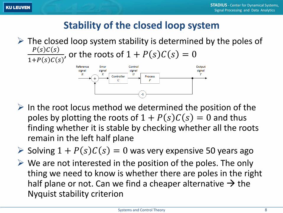
Stability of the closed loop system The closed loop system stability is determined by the poles of

𝑃𝑃 𝑠𝑠 𝐶𝐶 𝑠𝑠1+𝑃𝑃 𝑠𝑠 𝐶𝐶 𝑠𝑠

, or the roots of 1 + 𝑃𝑃 𝑠𝑠 𝐶𝐶 𝑠𝑠 = 0

In the root locus method we determined the position of the poles by plotting the roots of 1 + 𝑃𝑃 𝑠𝑠 𝐶𝐶 𝑠𝑠 = 0 and thus finding whether it is stable by checking whether all the roots remain in the left half plane

Solving 1 + 𝑃𝑃 𝑠𝑠 𝐶𝐶 𝑠𝑠 = 0 was very expensive 50 years ago We are not interested in the position of the poles. The only

thing we need to know is whether there are poles in the right half plane or not. Can we find a cheaper alternative the Nyquist stability criterion

8



Stability of the closed loop system: Nyquist criterion The Nyquist stability criterion avoids determining the roots of

1 + 𝑃𝑃 𝑠𝑠 𝐶𝐶 𝑠𝑠 exactly, it only determines the number of roots in the right half plane

It uses a theorem from complex calculus that finds the difference between the number of poles and the number of zeros within a contour (a closed curve)

We will apply this theorem to 1 + 𝑃𝑃 𝑠𝑠 𝐶𝐶 𝑠𝑠 (which can be seen as a complex function) and the contour will encircle the entire right half plane (= the Nyquist contour)

9



Complex function Before we get to the theorem that allows us to determine 𝑍𝑍 −𝑃𝑃 (the number of zeros – the number of poles within a contour), we have to show what a complex function is

A complex function 𝑓𝑓 𝑠𝑠 = 𝑢𝑢 𝑥𝑥,𝑦𝑦 + 𝑗𝑗 𝑣𝑣 𝑥𝑥,𝑦𝑦 maps the complex number 𝑠𝑠 = 𝑥𝑥 + 𝑗𝑗 𝑦𝑦 onto the complex number 𝑤𝑤 =𝑢𝑢 + 𝑗𝑗 𝑣𝑣

or for a contour:

The function 1 + 𝑃𝑃 𝑠𝑠 𝐶𝐶 𝑠𝑠 can also be regarded as a complex function, so we can use it as a mapping

𝑥𝑥

𝑦𝑦

𝑢𝑢

𝑣𝑣𝑓𝑓 𝑠𝑠

𝑥𝑥

𝑦𝑦

𝑢𝑢

𝑣𝑣𝑓𝑓 𝑠𝑠

10



Cauchy’s argument principle This is the engine behind the Nyquist stability criterion If a contour Γ in the 𝑠𝑠-plane circles 𝑍𝑍 zeros and 𝑃𝑃 poles of 𝑓𝑓 𝑠𝑠 in clock wise (CW) rotation, then the contour Γ′, which is the image of Γ as mapped by 𝑓𝑓 𝑠𝑠 , circles the origin (in the 𝑤𝑤-plane) 𝑍𝑍 − 𝑃𝑃 times in the clock wise (CW) direction

So the only thing we are looking at is the encirclements of the origin, all the other wiggles don’t matter to us

On the next slides we will prove this If you want to know more about this and related topics, we

refer you to the course ‘Complexe functieleer – 1st master WIT’

11



Cauchy’s argument principle

Let’s take a complex function 𝑓𝑓 𝑠𝑠 = 𝑠𝑠−𝑧𝑧1 𝑠𝑠−𝑧𝑧2 𝑠𝑠−𝑧𝑧3 …𝑠𝑠−𝑝𝑝1 𝑠𝑠−𝑝𝑝2 𝑠𝑠−𝑝𝑝3 …

So if we would apply this function to a complex number 𝑐𝑐 then this comes down to multiplying factors 𝑐𝑐 − 𝑧𝑧1 = 𝐴𝐴𝑧𝑧1𝑒𝑒𝑗𝑗𝜃𝜃𝑧𝑧1 and 1

𝑐𝑐−𝑝𝑝1= 1

𝐴𝐴𝑝𝑝1𝑒𝑒−𝑗𝑗𝜃𝜃𝑝𝑝1

So the modulus of 𝑓𝑓 𝑐𝑐 can be easily found by evaluating 𝐴𝐴𝑧𝑧1𝐴𝐴𝑧𝑧2𝐴𝐴𝑧𝑧3…𝐴𝐴𝑝𝑝1𝐴𝐴𝑝𝑝2𝐴𝐴𝑝𝑝3…

; this might help if you want to map a point, but it is

not important for usThe evaluation of the argument of 𝑓𝑓 𝑐𝑐 is what will be interesting; it is also very easy to find: ∠𝑓𝑓 𝑐𝑐 = 𝜃𝜃𝑧𝑧1 + 𝜃𝜃𝑧𝑧2 +𝜃𝜃𝑧𝑧3 + ⋯− 𝜃𝜃𝑝𝑝1 − 𝜃𝜃𝑝𝑝2 − 𝜃𝜃𝑝𝑝3 −⋯

12



Cauchy’s argument principleLet’s first show this graphically:

𝑓𝑓 𝑠𝑠

𝑥𝑥

𝑦𝑦

o

x

x𝜃𝜃𝑝𝑝1

𝜃𝜃𝑧𝑧1

𝜃𝜃𝑝𝑝2

𝐴𝐴𝑝𝑝2

𝐴𝐴𝑝𝑝1

𝐴𝐴𝑧𝑧1𝑢𝑢

𝑣𝑣

𝜃𝜃𝑝𝑝1𝜃𝜃𝑧𝑧1𝜃𝜃𝑝𝑝2

𝐴𝐴𝑝𝑝2

𝐴𝐴𝑝𝑝1

𝐴𝐴𝑧𝑧1𝐴𝐴𝑧𝑧1𝐴𝐴𝑝𝑝1𝐴𝐴𝑝𝑝2

𝜃𝜃𝑧𝑧1 − 𝜃𝜃𝑝𝑝1 − 𝜃𝜃𝑝𝑝2

13



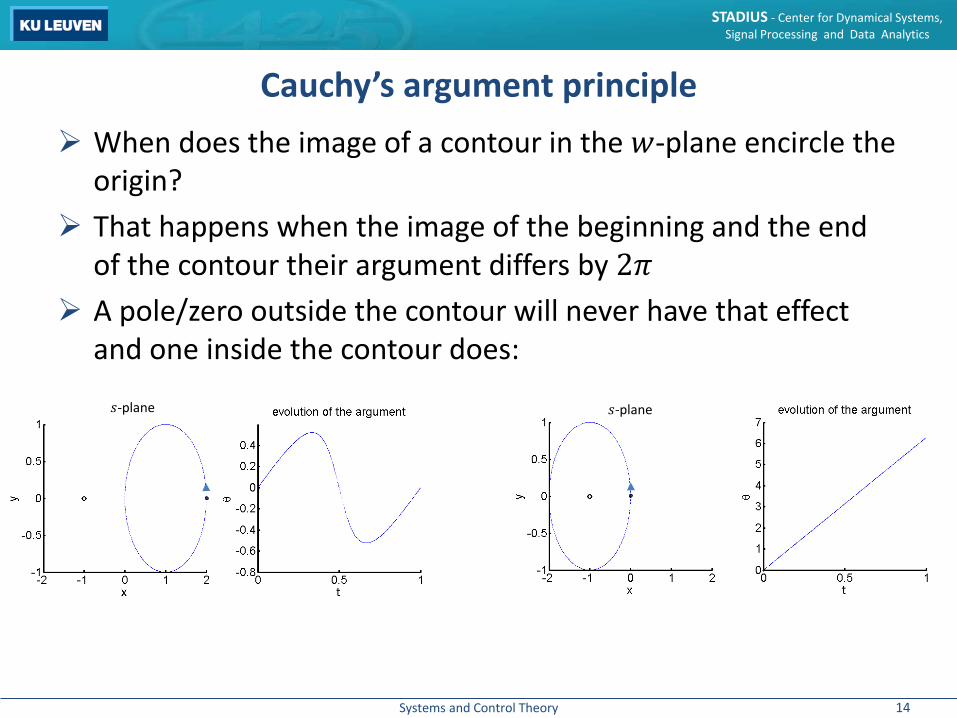
Cauchy’s argument principle When does the image of a contour in the 𝑤𝑤-plane encircle the

origin? That happens when the image of the beginning and the end

of the contour their argument differs by 2𝜋𝜋 A pole/zero outside the contour will never have that effect

and one inside the contour does:

𝑠𝑠-plane 𝑠𝑠-plane

14



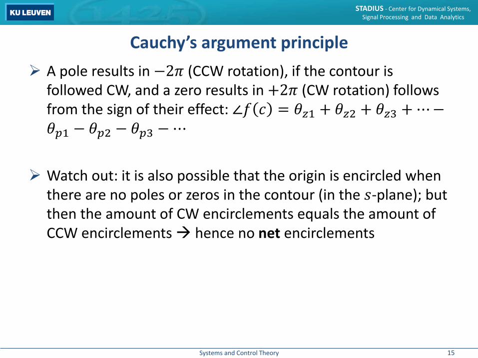
Cauchy’s argument principle A pole results in −2𝜋𝜋 (CCW rotation), if the contour is

followed CW, and a zero results in +2𝜋𝜋 (CW rotation) follows from the sign of their effect: ∠𝑓𝑓 𝑐𝑐 = 𝜃𝜃𝑧𝑧1 + 𝜃𝜃𝑧𝑧2 + 𝜃𝜃𝑧𝑧3 + ⋯−𝜃𝜃𝑝𝑝1 − 𝜃𝜃𝑝𝑝2 − 𝜃𝜃𝑝𝑝3 − ⋯

Watch out: it is also possible that the origin is encircled when there are no poles or zeros in the contour (in the 𝑠𝑠-plane); but then the amount of CW encirclements equals the amount of CCW encirclements hence no net encirclements

15



Cauchy’s argument principle: examplesTwo encircled poles (the x’s): 𝑃𝑃 = 2Four encircled zeros (the o’s): 𝑍𝑍 = 4Hence: 𝑁𝑁 = 𝑍𝑍 − 𝑃𝑃 = 2Indeed, the image of the contour encircles the origin twice in the𝑤𝑤-plane (in the CW direction)

𝑠𝑠-plane

16



Cauchy’s argument principle: examplesTwo encircled poles (the x’s): 𝑃𝑃 = 2One encircled zero (the o’s): 𝑍𝑍 = 1Hence: 𝑁𝑁 = 𝑍𝑍 − 𝑃𝑃 = −1Indeed, the image of the contour encircles the origin once in the𝑤𝑤-plane (in the CCW direction)

𝑠𝑠-plane

17



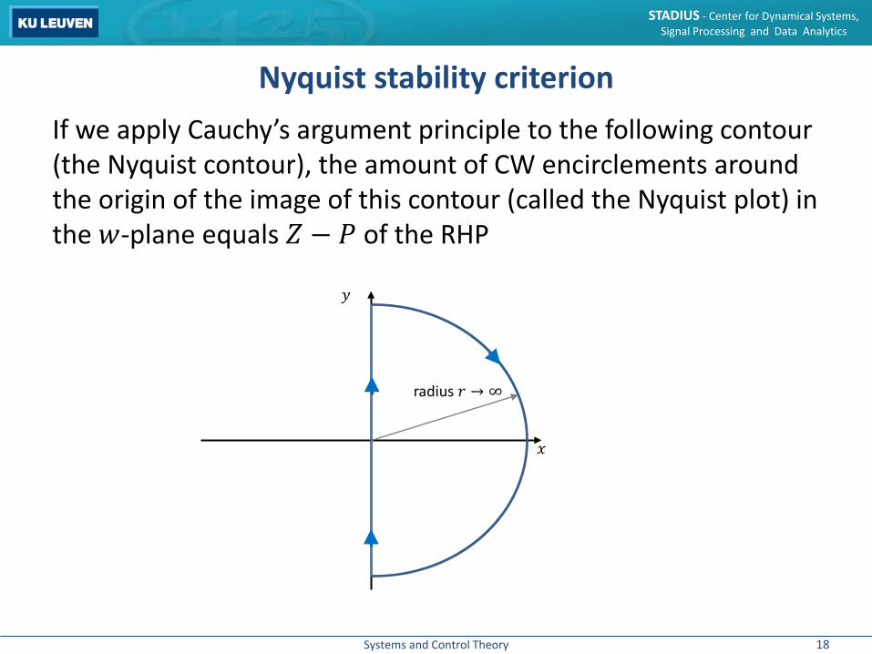
Nyquist stability criterionIf we apply Cauchy’s argument principle to the following contour (the Nyquist contour), the amount of CW encirclements around the origin of the image of this contour (called the Nyquist plot) in the 𝑤𝑤-plane equals 𝑍𝑍 − 𝑃𝑃 of the RHP

𝑥𝑥

radius 𝑟𝑟 → ∞

𝑦𝑦

18



Nyquist stability criterion That way we will find the difference between the number of

poles and zeros of 1 + 𝑃𝑃 𝑠𝑠 𝐶𝐶 𝑠𝑠 in the RHP: 𝑁𝑁 = 𝑍𝑍 − 𝑃𝑃 So if we now know 𝑃𝑃 (the number of poles in the RHP of 1 +𝑃𝑃 𝑠𝑠 𝐶𝐶 𝑠𝑠 ), we can know whether (and how many) zeros of 1 + 𝑃𝑃 𝑠𝑠 𝐶𝐶 𝑠𝑠 are in the RHP

Luckily this last aspect is simple; since the poles of 1 + 𝑃𝑃 𝑠𝑠 𝐶𝐶 𝑠𝑠equal those of 𝑃𝑃 𝑠𝑠 𝐶𝐶 𝑠𝑠 ; hence also the amount of RHP poles is equal (the connection between the zeros is not clear)

So if we assume the number of RHP poles of𝑃𝑃 𝑠𝑠 𝐶𝐶 𝑠𝑠 is known (which we’ll assume), we can know whether the system with unity feedback is stable

19



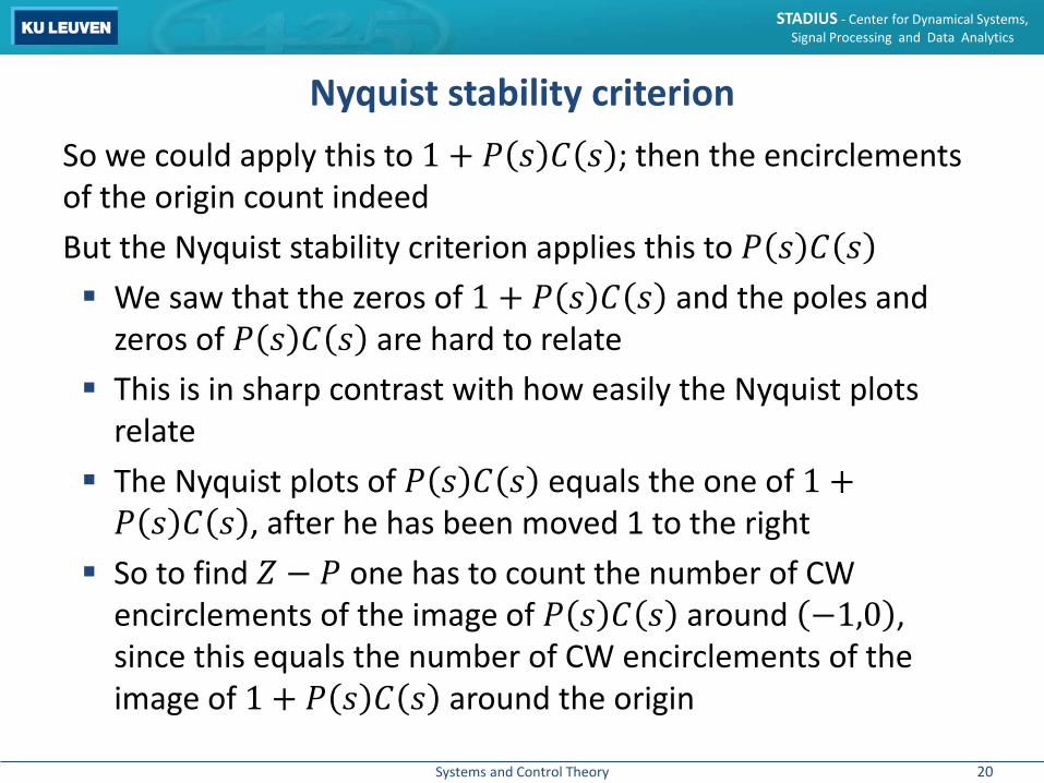
Nyquist stability criterionSo we could apply this to 1 + 𝑃𝑃 𝑠𝑠 𝐶𝐶 𝑠𝑠 ; then the encirclements of the origin count indeedBut the Nyquist stability criterion applies this to 𝑃𝑃 𝑠𝑠 𝐶𝐶 𝑠𝑠 We saw that the zeros of 1 + 𝑃𝑃 𝑠𝑠 𝐶𝐶 𝑠𝑠 and the poles and

zeros of 𝑃𝑃 𝑠𝑠 𝐶𝐶 𝑠𝑠 are hard to relate This is in sharp contrast with how easily the Nyquist plots

relate The Nyquist plots of 𝑃𝑃 𝑠𝑠 𝐶𝐶 𝑠𝑠 equals the one of 1 +𝑃𝑃 𝑠𝑠 𝐶𝐶 𝑠𝑠 , after he has been moved 1 to the right

So to find 𝑍𝑍 − 𝑃𝑃 one has to count the number of CW encirclements of the image of 𝑃𝑃 𝑠𝑠 𝐶𝐶 𝑠𝑠 around −1,0 , since this equals the number of CW encirclements of the image of 1 + 𝑃𝑃 𝑠𝑠 𝐶𝐶 𝑠𝑠 around the origin

20



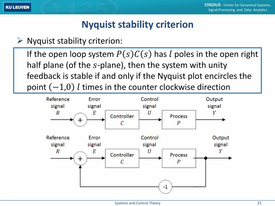
Nyquist stability criterion Nyquist stability criterion:

If the open loop system 𝑃𝑃 𝑠𝑠 𝐶𝐶 𝑠𝑠 has 𝑙𝑙 poles in the open right half plane (of the 𝑠𝑠-plane), then the system with unity feedback is stable if and only if the Nyquist plot encircles the point −1,0 𝑙𝑙 times in the counter clockwise direction

21



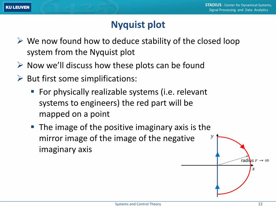
Nyquist plot We now found how to deduce stability of the closed loop

system from the Nyquist plot Now we’ll discuss how these plots can be found But first some simplifications: For physically realizable systems (i.e. relevant

systems to engineers) the red part will be mapped on a point

The image of the positive imaginary axis is themirror image of the image of the negativeimaginary axis

𝑥𝑥radius 𝑟𝑟 → ∞

𝑦𝑦

22



Nyquist plot: physically realizable systems Where does the very convenient property of physically

realizable systems come from? The reason is as follows:

1. Every physically realizable system is causal 2. Every causal system has a transfer function with an order of

the denominator that is larger than or equal to the order of the numerator

3. From this shape of the transfer function we can easily show that the red part maps onto a point


𝑦𝑦

23



Nyquist plot: physically realizable systems1. Every physically realizable system is causal

This is logical: you cannot build a system that knows the future

2. Every causal system has a transfer function with an order of the denominator that is larger than or equal to the order of the numerator

This can be easily understood in the discrete time case:𝑎𝑎0𝑦𝑦𝑛𝑛 + 𝑎𝑎1𝑦𝑦𝑛𝑛−1 + 𝑎𝑎2𝑦𝑦𝑛𝑛−2 + ⋯ = 𝑏𝑏0𝑢𝑢𝑛𝑛 +

𝑏𝑏1𝑢𝑢𝑛𝑛−1 + 𝑏𝑏2𝑢𝑢𝑛𝑛−2 + ⋯

𝐻𝐻 𝑧𝑧 = 𝑏𝑏0+𝑏𝑏1𝑧𝑧−1+𝑏𝑏2𝑧𝑧−2+⋯𝑎𝑎0+𝑎𝑎1𝑧𝑧−1+𝑎𝑎2𝑧𝑧−2+⋯

24



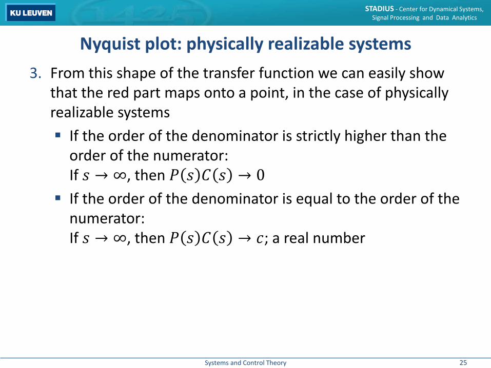
Nyquist plot: physically realizable systems3. From this shape of the transfer function we can easily show

that the red part maps onto a point, in the case of physically realizable systems If the order of the denominator is strictly higher than the

order of the numerator:If 𝑠𝑠 → ∞, then 𝑃𝑃 𝑠𝑠 𝐶𝐶 𝑠𝑠 → 0

If the order of the denominator is equal to the order of the numerator:If 𝑠𝑠 → ∞, then 𝑃𝑃 𝑠𝑠 𝐶𝐶 𝑠𝑠 → 𝑐𝑐; a real number

25



Nyquist plot; symmetry The symmetry follows directly from the way 𝑓𝑓 𝑐𝑐 can be

evaluated (see previously) Since the position of 𝑓𝑓 𝑐𝑐 only depends on the location of the

poles and zeros, and those poles and zeros only occur symmetrically round the real axis; the Nyquist plot will be symmetrical round the real axis

26



Nyquist plot So we will only have to study the positive (or the negative)

imaginary axis! The circular part maps onto one point, which is the same

as where 𝑗𝑗𝜔𝜔 maps onto The other half of the imaginary axis will give the mirror

image of the studied half

𝑥𝑥

𝑦𝑦


𝑦𝑦

27



Nyquist plot Extracting the number of times −1,0 is circled now isn’t that

difficult anymore; You search for the image of 𝑗𝑗𝑗+

You search for the image of 𝑗𝑗∞ Then you search for the positive real 𝑦𝑦 for which 𝑓𝑓 𝑗𝑗𝑦𝑦 ’s

imaginary part changes sign This information allows you to determine if you encircle

−1,0 Let’s show this with a simple example; but of course you can

use software to do this! (e.g. nyquist in Matlab)

28



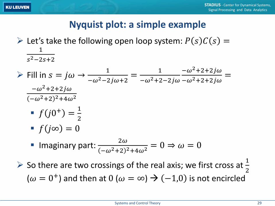
Nyquist plot: a simple example Let’s take the following open loop system: 𝑃𝑃 𝑠𝑠 𝐶𝐶 𝑠𝑠 =

1𝑠𝑠2−2𝑠𝑠+2

Fill in 𝑠𝑠 = 𝑗𝑗𝜔𝜔 → 1−𝜔𝜔2−2𝑗𝑗𝜔𝜔+2

= 1−𝜔𝜔2+2−2𝑗𝑗𝜔𝜔

−𝜔𝜔2+2+2𝑗𝑗𝜔𝜔−𝜔𝜔2+2+2𝑗𝑗𝜔𝜔

=−𝜔𝜔2+2+2𝑗𝑗𝜔𝜔−𝜔𝜔2+2 2+4𝜔𝜔2

𝑓𝑓 𝑗𝑗𝑗+ = 12

𝑓𝑓 𝑗𝑗∞ = 0

Imaginary part: 2𝜔𝜔−𝜔𝜔2+2 2+4𝜔𝜔2 = 0 ⇒ 𝜔𝜔 = 0

So there are two crossings of the real axis; we first cross at 12

(𝜔𝜔 = 0+) and then at 0 (𝜔𝜔 = ∞) −1,0 is not encircled

29



Nyquist plot: a simple example

Remember our open loop system: 𝑃𝑃 𝑠𝑠 𝐶𝐶 𝑠𝑠 = 1𝑠𝑠2−2𝑠𝑠+2

𝑍𝑍 and 𝑃𝑃 are the number of zeros and poles of 1 + 𝑃𝑃 𝑠𝑠 𝐶𝐶 𝑠𝑠 The poles of 𝑃𝑃 𝑠𝑠 𝐶𝐶 𝑠𝑠 and 1 + 𝑃𝑃 𝑠𝑠 𝐶𝐶 𝑠𝑠 are the same

𝑃𝑃 = 2 in our simple example Since −1,0 is not encircled: Z − 𝑃𝑃 = 0; hence there are 2

zeros in the right half plane Remember that the zeros of 1 + 𝑃𝑃 𝑠𝑠 𝐶𝐶 𝑠𝑠 are the poles of

the closed loop system and thus, the unity feedback controller is unstable

30



Nyquist plot: poles on the imaginary axis There is one more thing to Nyquist plots: how to deal with

poles on the imaginary axis Why are they a problem? Take for instance the case with one pair

of imaginary poles at 𝑗𝑗𝑐𝑐 and −𝑗𝑗𝑐𝑐 When coming close to 𝑗𝑗𝑐𝑐 the argument

will remain 0 and the gain will increase to infinity

At 𝑗𝑗𝑐𝑐 itself the gain will be infinite, but the argument isundetermined, hence we cannot map this point

𝑥𝑥

𝑦𝑦

x

x

31



Nyquist plot: poles on the imaginary axis How to solve this? Instead of going through the poles, we will evade them by

an infinitesimally small amount That way we do not have the problem of an

undetermined mapping at the pole Since we avoid them by an infinitesimally

small amount we also know we will not wrongly avoid a pole that lies in the right half plane

Now the Nyquist plot will go to infinity as x is approached, then the argument will change from 0 to 𝜋𝜋 as the semi-circle is traversed and then the Nyquist plot will return from infinity

s

𝑥𝑥

𝑦𝑦

x

x

radius 𝜖𝜖 → 0

32



The Nyquist criterion in the discrete time case The Cauchy argument principle still applies, since 𝑃𝑃 𝑧𝑧 𝐶𝐶 𝑧𝑧

also has the shape of a rational polynomial The contour now will have to encircle the entire complex

plane except for the unity circle

𝑥𝑥

𝑦𝑦

1

1 radius 𝑟𝑟 → ∞

33



The Nyquist criterion in the discrete time case This is not a contour however, but this can be solved with the

following trick:

With the two horizontal pieces both infinitely close to the real axis, that way they are identical but with opposite signs, so they will cancel each other

𝑥𝑥

𝑦𝑦

radius 𝑟𝑟 → ∞1

1

34



Margins The Nyquist plot allows us to determine ‘how stable’ the

system will be We know that the stability changes when 1 + 𝑃𝑃 𝑠𝑠 𝐶𝐶 𝑠𝑠 has

an imaginary zero (then the system is marginally stable) Can we see such a zero in the Nyquist plot of 𝑃𝑃 𝑠𝑠 𝐶𝐶 𝑠𝑠 ? Of course; the Nyquist plot is the image of the imaginary axis,

so if there is a zero on the imaginary axis, the Nyquist plot of 1 + 𝑃𝑃 𝑠𝑠 𝐶𝐶 𝑠𝑠 would go through 0 and the Nyquist plot of 𝑃𝑃 𝑠𝑠 𝐶𝐶 𝑠𝑠 will go through −1

Hence the system is marginally stable if the Nyquist plot goes through −1

35



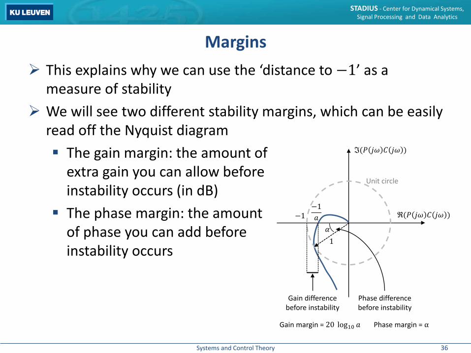
Margins This explains why we can use the ‘distance to −1’ as a

measure of stability We will see two different stability margins, which can be easily

read off the Nyquist diagram The gain margin: the amount of

extra gain you can allow before instability occurs (in dB)

The phase margin: the amount of phase you can add before instability occurs

−1−1𝑎𝑎

Gain difference before instability

𝛼𝛼1

Phase difference before instability

ℑ(𝑃𝑃 𝑗𝑗𝜔𝜔 𝐶𝐶 𝑗𝑗𝜔𝜔 )

ℜ(𝑃𝑃 𝑗𝑗𝜔𝜔 𝐶𝐶 𝑗𝑗𝜔𝜔 )

Unit circle

Gain margin = 20 log10 𝑎𝑎 Phase margin = α

36



Margins: gain margin The gain margin is the amount of extra gain allowed before

the system becomes unstable Or: how much larger the gain has to be, before the system

becomes unstable The gain margin is multiplicative, so it is the factor with which

you have to multiply the gain so the Nyquist plot goes through − 1 in the 𝑤𝑤-plane

It will be expressed in dB; take 𝐾𝐾 a certain factor, then this can be expressed in dB as follows: 20 ⋅ log10 𝐾𝐾 dB

37



Margins: gain margin Let’s look at this the following way:

The stability margin of 𝑃𝑃 𝑠𝑠 with unity feedback is the 𝐾𝐾 for which the system above is marginally stable

𝐾𝐾 𝑃𝑃 𝑠𝑠+𝑅𝑅 𝑠𝑠

-1

𝐸𝐸 𝑠𝑠 𝑈𝑈 𝑠𝑠 𝑌𝑌 𝑠𝑠

38



Margins: gain margin So 𝐾𝐾𝑃𝑃 𝑠𝑠 should equal −1 for an imaginary 𝑠𝑠 = 𝑗𝑗𝜔𝜔 This requires ∠ 𝐾𝐾𝑃𝑃 𝑗𝑗𝜔𝜔 = ∠𝑃𝑃 𝑗𝑗𝜔𝜔 to equal −180°; this 𝜔𝜔𝜋𝜋

is called the gain crossover frequency (GCF) 𝐾𝐾 then has to be set such that 𝐾𝐾𝑃𝑃 𝑗𝑗𝜔𝜔𝜋𝜋 = 1 So now you should be able to understand that a large gain can

lead to instability; and that this risk only exists when there exists a 𝜔𝜔𝜋𝜋 for which ∠𝑃𝑃 𝑗𝑗𝜔𝜔 = −180°

We will illustrate this with a few examples

39



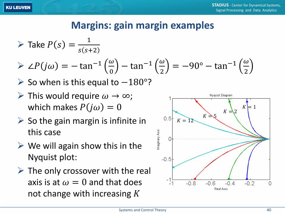
Margins: gain margin examples

Take 𝑃𝑃 𝑠𝑠 = 1𝑠𝑠 𝑠𝑠+2

∠𝑃𝑃 𝑗𝑗𝜔𝜔 = − tan−1 𝜔𝜔0− tan−1 𝜔𝜔

2= −90° − tan−1 𝜔𝜔

2 So when is this equal to −180°? This would require 𝜔𝜔 → ∞;

which makes 𝑃𝑃 𝑗𝑗𝜔𝜔 = 0 So the gain margin is infinite in

this case We will again show this in the

Nyquist plot: The only crossover with the real

axis is at 𝜔𝜔 = 0 and that does not change with increasing 𝐾𝐾

𝐾𝐾 = 1𝐾𝐾 = 2

𝐾𝐾 = 5𝐾𝐾 = 12

40



Margins: phase margin The phase margin is how much you can rotate the Nyquist

diagram before −1 is crossed This can be interpreted as multiplying 𝑃𝑃 𝑠𝑠 with 𝑒𝑒𝑗𝑗𝜃𝜃 until −1

is crossed So 𝑃𝑃 𝑠𝑠 𝑒𝑒𝑗𝑗𝜃𝜃 = −1 for an imaginary 𝑠𝑠 = 𝑗𝑗𝜔𝜔 This requires 𝑃𝑃 𝑗𝑗𝜔𝜔 𝑒𝑒𝑗𝑗𝜃𝜃 = 𝑃𝑃 𝑗𝑗𝜔𝜔 to equal 1; this 𝜔𝜔0 is

called the phase crossover frequency (PCF) 𝜃𝜃 then has to be set such that ∠ 𝑃𝑃 𝑠𝑠 𝑒𝑒𝑗𝑗𝜃𝜃 = ∠𝑃𝑃 𝑠𝑠 + 𝜃𝜃 =− 180°

The gain margin is defined as positive, but that doesn’t matter, because of the symmetry with respect to the real axis: If a rotation of 𝜃𝜃 degrees results in a crossing of −1, then a

rotation of −𝜃𝜃 does the same

41



Margins: phase margin

Let’s take 𝑃𝑃 𝑠𝑠 = 1𝑠𝑠 𝑠𝑠+2

again

When is 𝑃𝑃 𝑗𝑗𝜔𝜔 = 1?1𝜔𝜔⋅ 1

𝜔𝜔2+4= 1, hence 𝜔𝜔4 + 4𝜔𝜔2 = 1, or 𝜔𝜔 = 5 − 2 = 0.486

Find 𝜃𝜃 such that ∠ 𝑃𝑃 𝑗𝑗𝜔𝜔 𝑒𝑒𝑗𝑗𝜃𝜃 = −180°

𝜃𝜃 = −180° + tan−1 𝜔𝜔0

+ tan−1 𝜔𝜔2

= −76.34°

The phase margin is 76.34°

42



Margins: phase margin We’ll show this graphically with the Nyquist plot again:

76.34°

43



Margins: what should the margins be? Gain margin: If it is too small the real system might be unstable, since

several practical factors increase instability Increasing the gain margin, makes the system slower So we have to take the gain margin large enough to be

safe, but not too large It should definitely be larger than 3 dB A value larger than 15 dB makes for a quite conservative

design normally

! A large gain margin does not provide certainty that the ! system will be stable; on the other hand, if the gain margin is ! very low, you can be fairly certain of instability

44



Margins: what should the margins be? Phase margin: This is more subtle than the gain margin If it is too small instability might again occur due to

practicalities If it is too small we get large overshoots and large

oscillations that fade away very slowly; which is not something we associate with a good form of stability

Sometimes a good value is 60°, but it is highly case dependent

! Again, a good margin does not offer certainty about the stability; whereas a bad phase margin (very large or very small) does give certainty about instability

45



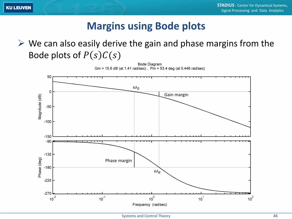
Margins using Bode plots We can also easily derive the gain and phase margins from the

Bode plots of 𝑃𝑃 𝑠𝑠 𝐶𝐶(𝑠𝑠)

Gain margin

Phase margin

𝜔𝜔0

𝜔𝜔𝜋𝜋

46



Margins: design example We’ll design a simple proportional controller for the system 𝑃𝑃 𝑠𝑠 = 1−𝑠𝑠

1+𝑠𝑠 2

What will 𝐾𝐾 have to be in order to have a phase margin of 45°?

𝐾𝐾 𝑃𝑃 𝑠𝑠+𝑅𝑅 𝑠𝑠

-1

𝐸𝐸 𝑠𝑠 𝑈𝑈 𝑠𝑠 𝑌𝑌 𝑠𝑠

47



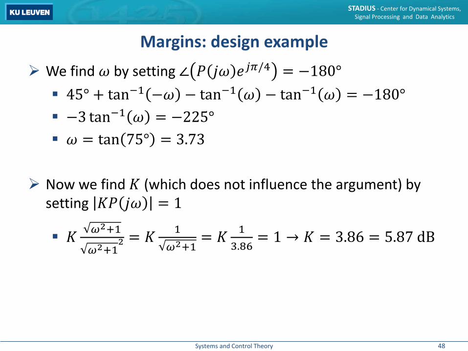
Margins: design example We find 𝜔𝜔 by setting ∠ 𝑃𝑃 𝑗𝑗𝜔𝜔 𝑒𝑒𝑗𝑗𝜋𝜋/4 = −180° 45° + tan−1 −𝜔𝜔 − tan−1 𝜔𝜔 − tan−1 𝜔𝜔 = −180° −3 tan−1 𝜔𝜔 = −225° 𝜔𝜔 = tan 75° = 3.73

Now we find 𝐾𝐾 (which does not influence the argument) by setting 𝐾𝐾𝑃𝑃 𝑗𝑗𝜔𝜔 = 1

𝐾𝐾 𝜔𝜔2+1

𝜔𝜔2+12 = 𝐾𝐾 1

𝜔𝜔2+1= 𝐾𝐾 1

3.86= 1 → 𝐾𝐾 = 3.86 = 5.87 dB

48



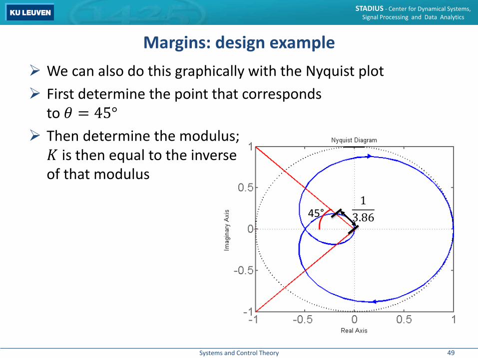
Margins: design example We can also do this graphically with the Nyquist plot First determine the point that corresponds

to 𝜃𝜃 = 45° Then determine the modulus;𝐾𝐾 is then equal to the inverseof that modulus

45°1

3.86

49



Let’s recapitulate The Nyquist stability criterion came to existence as a cheap

alternative to determine stability of a closed loop system with unity feedback

It also allows to see the phase margin and the gain margin; which are a measure of how stable the system actually is

It’s relevance today is as a design tool, as shown in the final example

In the next section we will discuss new kinds of classical control components

Bode plots make up a similar tool, yet the Nyquist stability criterion is (slightly) more generally applicable

50



Interesting links About the Nyquist argument principle: https://www.youtube.com/watch?v=sof3meN96MA&inde

x=3&list=PLEJyHgf7y0ie3nwSzMDVzAdxf4dK9m89a https://www.youtube.com/watch?v=tsgOstfoNhk

About margins: https://www.youtube.com/watch?v=Hw_hrxsX4_M https://www.youtube.com/watch?v=BTNZ8SRs7Y8 https://www.youtube.com/watch?v=V1mfy7VhJNQ

51

https://www.youtube.com/watch?v=sof3meN96MA&index=3&list=PLEJyHgf7y0ie3nwSzMDVzAdxf4dK9m89a

https://www.youtube.com/watch?v=tsgOstfoNhk

https://www.youtube.com/watch?v=Hw_hrxsX4_M

https://www.youtube.com/watch?v=BTNZ8SRs7Y8

https://www.youtube.com/watch?v=V1mfy7VhJNQ

design in the frequency domain nyquist stability criterionmaapc/static/files... · nyquist plot we...

Documents