design of digital filters

Chapter 8

Design of Digital Filters

Contents

Overview . . . . . . . . . . . . . . . . . . . . . . . . . . . . . . . . . . . . . . . . . . . . . . . . . . . . . . . . 8.2General Considerations . . . . . . . . . . . . . . . . . . . . . . . . . . . . . . . . . . . . . . . . . . . . . . . . . 8.2Design of FIR Filters . . . . . . . . . . . . . . . . . . . . . . . . . . . . . . . . . . . . . . . . . . . . . . . . . . 8.4Design of linear-phase FIR filters using windows . . . . . . . . . . . . . . . . . . . . . . . . . . . . . . . . . . . . 8.7Time-delay in desired response . . . . . . . . . . . . . . . . . . . . . . . . . . . . . . . . . . . . . . . . . . . . . 8.9Sidelobes . . . . . . . . . . . . . . . . . . . . . . . . . . . . . . . . . . . . . . . . . . . . . . . . . . . . . . . . 8.10Hilbert transform (90◦ phase shift) . . . . . . . . . . . . . . . . . . . . . . . . . . . . . . . . . . . . . . . . . . . 8.12Design of FIR filters by frequency sampling . . . . . . . . . . . . . . . . . . . . . . . . . . . . . . . . . . . . . . 8.12“Optimum” equiripple linear-phase FIR filters . . . . . . . . . . . . . . . . . . . . . . . . . . . . . . . . . . . . . 8.14Comparison of FIR methods . . . . . . . . . . . . . . . . . . . . . . . . . . . . . . . . . . . . . . . . . . . . . . . 8.17Design of IIR Filters from Analog Filters . . . . . . . . . . . . . . . . . . . . . . . . . . . . . . . . . . . . . . . . 8.18IIR filter design by bilinear transformation . . . . . . . . . . . . . . . . . . . . . . . . . . . . . . . . . . . . . . . 8.19Frequency Transformations . . . . . . . . . . . . . . . . . . . . . . . . . . . . . . . . . . . . . . . . . . . . . . . 8.24Design of Digital Filters Based on Least-Squares Method . . . . . . . . . . . . . . . . . . . . . . . . . . . . . . . 8.24Summary . . . . . . . . . . . . . . . . . . . . . . . . . . . . . . . . . . . . . . . . . . . . . . . . . . . . . . . . 8.24

8.1

8.2 c© J. Fessler, May 27, 2004, 13:18 (student version)

So far our treatment of DSP has focused primarily on the analysis of discrete-time systems. Now we finally have the analyticaltools to begin to design discrete-time systems. All LTI systems can be thought of as filters, so, at least for LTI systems, to “design”a system means to design a digital filter.

(The design of nonlinear or time-varying systems is generally more complicated, and often more case specific.)

Goal: given desired• magnitude response |Hd(ω) |• phase response ∠Hd(ω)• tolerance specifications (how far from ideal?),

we want to choose the filter parameters N , M , {ak}, {bk} such that the system function

H(z) =

∑Mk=0 bkz−1

∑Nk=0 akz−1

= g

∏

i(z − zi)∏

j(z − pj),

where a0 = 1, yields a frequency response H(ω) ≈ Hd(ω).

Rational H(z), so LTI system described by a constant-coefficient difference equation, so can be implemented with finite # of adds,multiplies, and delays.

In other words, filter design means choosing the number and locations of the zeros and poles, or equivalently the number andvalues of the filter coefficients, and thus H(z), h[n], H(ω).

Overview• N = 0, FIR or all-zero. linear passband phase.• N > 0, IIR. lower sidelobes for same number of coefficients.

8.1General Considerations• Ideally would like N and M or N + M to be as small as possible for minimal computation / storage.• Causal (for now)• Poles inside unit circle for stability

8.1.1 Causality

We will focus on designing causal digital filters, since those can be implemented in real time. Noncausal filter design (e.g., foroff-line applications) is much easier and many of the same principles apply anyway.

An LTI system is causal iff• input/output relationship: y[n] depends only on current and past input signal values.• impulse response: h[n] = 0 for n < 0• system function: number of finite zeros ≤ number of finite poles• frequency response: What can we say about H(ω)?

Fact: if h[n] is causal, then• Paley-Wiener Theorem: H(ω) cannot be exactly zero over any band of frequencies. (Except in the trivial case where h[n] = 0.)• Furthermore, |H(ω)| cannot be flat (constant) over any finite band.• HR(ω) and HI(ω) are Hilbert transform pairs. Therefore they are not independent. Hence magnitude and phase response are

interdependent.

Thus those ideal filters with finite bands of zero response cannot be implemented with a causal filter.

Instead, we must design filters that approximate the desired frequency response Hd(ω).

c© J. Fessler, May 27, 2004, 13:18 (student version) 8.3

8.1.2 Characteristics of practical frequency-selective filters

No perfectly flat regions

Fact: since causal filters cannot have a band of frequencies with zero response, nor can they have any band of frequencies overwhich the frequency response is a constant.

Proof by contradiction. Suppose H(ω) = c for ω1 ≤ ω ≤ ω2, with corresponding impulse response h[n]. Now define a new filterg[n] = h[n]−c δ[n]. Then certainly g[n] is also causal. But G(ω) = H(ω)−c = 0 for ω1 ≤ ω ≤ ω2, which is impossible if g[n]is causal. �

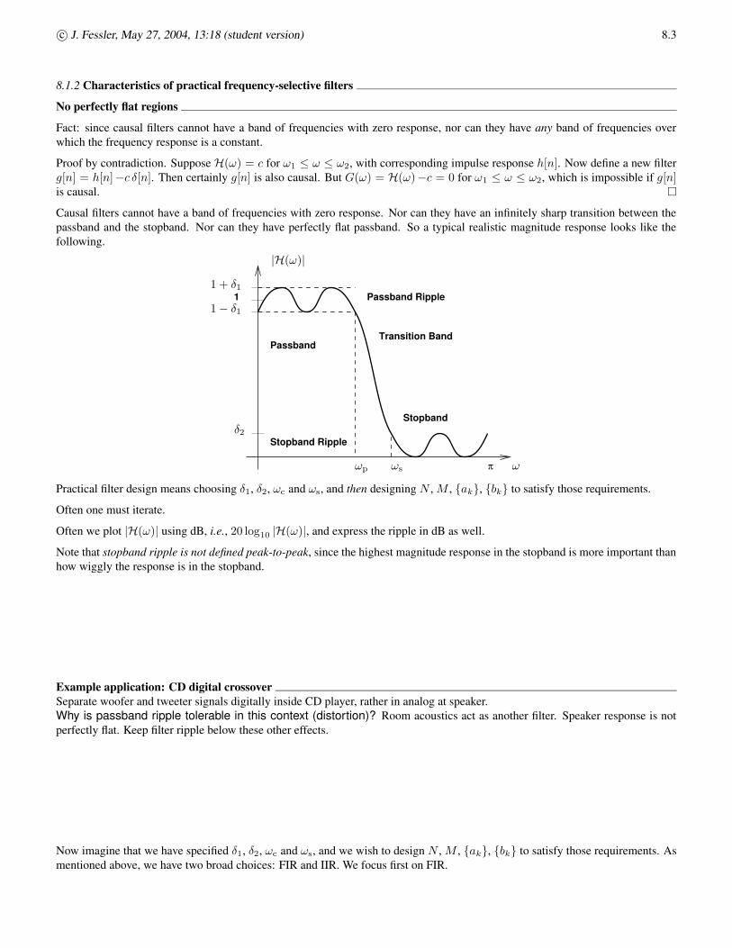
Causal filters cannot have a band of frequencies with zero response. Nor can they have an infinitely sharp transition between thepassband and the stopband. Nor can they have perfectly flat passband. So a typical realistic magnitude response looks like thefollowing.

π

Stopband Ripple

Passband

Stopband

1

Transition Band

Passband Ripple

PSfrag replacements

1 + δ1

1 − δ1

ωp ωs

δ2

ω

|H(ω)|

Practical filter design means choosing δ1, δ2, ωc and ωs, and then designing N , M , {ak}, {bk} to satisfy those requirements.

Often one must iterate.

Often we plot |H(ω)| using dB, i.e., 20 log10 |H(ω)|, and express the ripple in dB as well.

Note that stopband ripple is not defined peak-to-peak, since the highest magnitude response in the stopband is more important thanhow wiggly the response is in the stopband.

Example application: CD digital crossoverSeparate woofer and tweeter signals digitally inside CD player, rather in analog at speaker.Why is passband ripple tolerable in this context (distortion)? Room acoustics act as another filter. Speaker response is notperfectly flat. Keep filter ripple below these other effects.

Now imagine that we have specified δ1, δ2, ωc and ωs, and we wish to design N , M , {ak}, {bk} to satisfy those requirements. Asmentioned above, we have two broad choices: FIR and IIR. We focus first on FIR.


8.2Design of FIR Filters

An FIR filter of length M is an LTI system with the following difference equation1:

y[n] =

M−1∑

k=0

bk x[n − k] .

Note that the book changes the role of M here. Earlier, when discussing rational system functions, M was the number of zeros.Now M is the number of “nonzero” elements of h[n], which corresponds to at most M − 1 zeros. (More precisely, we assumebM−1 6= 0 and b0 6= 0, but some of the coefficients in between could be zero.)

The problem: given δ1, δ2, ωc, and ωs, we wish to choose M and {bk}M−1k=0 to achieve that goal.

We focus on linear-phase FIR filters, because if linear phase is not needed, then IIR is probably preferable anyway.

We focus on lowpass filters, since transformations can be made to form highpass, bandpass from lowpass, as discussed previously.

Impulse response

Clearly for an FIR filter

h[n] =

{

bn, n = 0, . . . ,M − 10, otherwise.

So rather than writing everything in terms of bk’s, we write it directly in terms of the impulse response h[n].

In fact, for FIR filter design we usually design h[n] directly, rather than starting from a pole-zero plot.(An exception would be notch filters.)

8.2.1 Symmetric and antisymmetric FIR filters

I focus on the symmetric case.

System function:

H(z) =

M−1∑

n=0

h[n] z−n.

How do we make a filter have linear phase?We previously answered this in the pole-zero domain. Now we examine it in the time domain.

An FIR filter has linear phase if h[n] = h[M − 1 − n], n = 0, 1, . . . ,M − 1.

Example. For M = 5: h[n] = {b0, b1, b2, b1, b0} .

Such an FIR filter is called symmetric. Caution: this is not “even symmetry” though in the sense we discussed previously.

This is related, but not exactly the same as circular symmetry.

Example. For M = 3 and h[n] ={

1/2, 1, 1/2}

. Does this filter have linear phase? Is it lowpass or highpass?

H(ω) =1

2+ e−ω +

1

2e−2ω = e−ω

[

1

2eω + 1 +

1

2e−ω

]

= e−ω (1 + cosω),

so since 1 + cosω ≥ 0, ∠H(ω) = −ω, which is linear phase.

So it works for this particular example, but why does the symmetry condition ensure linear phase in general?

1Caution. At this point the book switches from∑

M

k=0to

∑

M−1

k=0apparently. This inconsistent with MATLAB, so there are “M − 1” factors that appear

frequently in the MATLAB calls. I think that MATLAB is consistent and the book makes an undesirable switch of convention here.


Symmetric real FIR filters, h[n] = h[M − 1 − n], n = 0, . . . , M − 1, are linear phase.

Proof. Suppose M is even:

H(z) =M−1∑

n=0

h[n] z−n

=

M/2−1∑

n=0

h[n] z−n +M−1∑

n=M/2

h[n] z−n (split sum)

=

M/2−1∑

n=0

h[n] z−n +

M/2−1∑

n′=0

h[M − 1 − n′] z−(M−1−n′) (n′ = M − 1 − n)

=

M/2−1∑

n=0

h[n] z−n +

M/2−1∑

n=0

h[n] z−(M−1−n) (symmetry of h[n])

=

M/2−1∑

n=0

h[n][

z−n + z−(M−1−n)]

(combine)

= z−(M−1)/2

M/2−1∑

n=0

h[n][

z(M−1)/2−n + z−((M−1)/2−n)]

(split phase).

Thus the frequency response is

H(ω) = H(z)∣

∣

∣

z=eω

= e−ω(M−1)/2

M/2−1∑

n=0

h[n][

eω((M−1)/2−n) + e−ω((M−1)/2−n)]

= 2 e−ω(M−1)/2

M/2−1∑

n=0

h[n] cos

[

ω

(

M − 1

2− n

)]

= e−ω(M−1)/2 Hr(ω)

Hr(ω) = 2

M/2−1∑

n=0

h[n] cos

[

ω

(

M − 1

2− n

)]

. (Real since h[n] is real.)

Phase response:

∠H(ω) =

{

−ωM−12 , Hr(ω) > 0

−ωM−12 + π, Hr(ω) < 0.

The case for M odd is similar, and leads to the same phase response but with a slightly different Hr(ω).


In fact, the odd M case is even easier by noting that h[n + (M − 1)/2] is an even function, so its DTFT is real, so the DTFT ofh[n] is e−ω(M−1)/2 times a real function. This proof does not work for M even since then (M − 1)/2 is not an integer so wecannot use the shift property.

What about pole-zero plot? (We want to be able to recognize FIR linear-phase filters from pole-zero plot.)

From above, H(z) = z−(M−1)/2∑M/2−1

n=0 h[n][

z(M−1)/2−n + z−((M−1)/2−n)]

soH

(

z−1)

= z(M−1)/2∑M/2−1

n=0 h[n][

z−(M−1)/2−n + z((M−1)/2−n)]

= zM−1 H(z) . Thus

H(z) = z−(M−1) H(

z−1)

.

So if q is a zero of H(z), then 1/q is also a zero of H(z). Furthermore, in the usual case where h[n] is real, if q is a zero of H(z),then so is q∗.

Example. Here are two pole-zero plots of such linear-phase filters.

Re(z)

Im(z)

2

r 1r

Re(z)

Im(z)

4

What is difference between this and all-pass filter? It was poles and zeros in reciprocal relationships for all-pass filter.

Now we know conditions for FIR filters to be linear phase. How do we design one?

Delays

In continuous time, the delay property of the Laplace transform is

xa(t − τ)L↔ e−sτ Xa(s) .

How do we build a circuit that delays a signal? Since e−sτ is not a rational function, so it cannot be implemented exactly usingRLC circuits. So even though a time delay system is an LTI system, we cannot build it using RLC components!

We can make an approximation, e.g.,

e−sτ ≈ 1 − sτ +1

2s2τ2

which is rational in s, so we can design such an RLC circuit.

Or, we can use more mechanical approaches to delay like a tape loop. Picture . write, read, erase head. delay ∝ 1 / tape velocity.

Another approach is to rely on signal propagation time down a long wire, and tap into the wire at various places for various delays.

What about in discrete time? We just need a digital latch or buffer (flip flops) to hold the bits representing a digital signal valueuntil the next time point.


8.2.2Design of linear-phase FIR filters using windows

Perhaps the simplest approach to FIR filter design is to take the ideal impulse response hd[n] and truncate it, which meansmultiplying it by a rectangular window, or more generally, to multiply hd[n] by some other window function, where

hd[n] =1

2π

∫ π

−π

Hd(ω) eωn dω .

Typically hd[n] will be noncausal or at least non-FIR.

Example. As shown previously, if Hd(ω) =

{

1, |ω| ≤ ωc,0, otherwise,

= rect(

ω2ωc

)

then hd[n] =ωc

πsinc

(ωc

πn)

.

We can create an FIR filter by windowing the ideal response:

h[n] = w[n] hd[n] =

{

hd[n] w[n], n = 0, . . . ,M − 10, otherwise,

where the window function w[n] is nonzero only for n = 0, . . . ,M − 1.

What is the effect on the frequency response?

W(ω) =

M−1∑

n=0

w[n] e−ωn

and by time-domain multiplication property of DTFT, aka the windowing theorem:

H(ω) = W(ω) ©2π Hd(ω) =1

2π

∫ π

−π

Hd(λ)W(ω − λ) dλ, (8-1)

where ©2π denotes 2π-periodic convolution.

In words, the ideal frequency response Hd(ω) is smeared out by the frequency response W(ω) of the window function.

What would the frequency response of the “ideal” window be? W(ω) = “2π δ(ω) ” =∑∞

k=−∞ 2π δ(ω − 2πk), a Diracimpulse. Such a “window” would cause no smearing of the ideal frequency response.

However, the corresponding “window” function would be w[n] = 1, which is noncausal and non-FIR.

So in practice we must make tradeoffs.

Example. rectangular window. w[n] =

{

1, n = 0, . . . , 20, otherwise,

with Hd(ω) = e−ω 2 rect(

ωπ

)

, i.e., ωc = π/2.

So by the shift property of the DTFT: hd[n] = sinc(

12 (n − 1

)

) and h[n] ={

sinc(

12

)

, 1, sinc(

12

)

}

where sinc(

12

)

= 2/π ≈ 0.64.

So the resulting frequency response is H(ω) = e−ω[

1 + 4π cos(ω)

]

. Picture

This is only a 3-tap design. Let us generalize next.


Example. rectangular window.

w[n] =

{

1, n = 0, . . . ,M − 10, otherwise,

W(ω) =

M−1∑

n=0

e−ωn = · · · = e−ω(M−1)/2 Wr(ω), where Wr(ω) =

sin(ωM/2)

sin(ω/2), ω 6= 0

M, ω = 0.

In this case the ideal frequency response is smeared out by a sinc-like function, because Wr(ω) ≈ M sinc(

M ω2π

)

.

The function sin(ωM/2)M sin(ω/2) is available in MATLAB as the diric function: the Dirichlet or periodic sinc function.

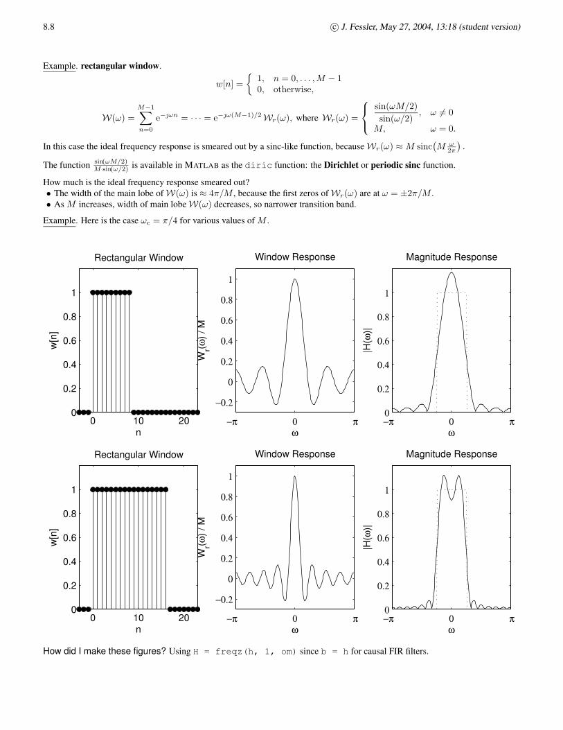
How much is the ideal frequency response smeared out?• The width of the main lobe of W(ω) is ≈ 4π/M , because the first zeros of Wr(ω) are at ω = ±2π/M .• As M increases, width of main lobe W(ω) decreases, so narrower transition band.

Example. Here is the case ωc = π/4 for various values of M .

0 10 200

0.2

0.4

0.6

0.8

1

n

w[n

]

Rectangular Window

−π 0 π

−0.2

0

0.2

0.4

0.6

0.8

1

ω

Wr(ω

) / M

Window Response

−π 0 π0

0.2

0.4

0.6

0.8

1

ω

|H(ω

)|

Magnitude Response

0 10 200

0.2

0.4

0.6

0.8

1

n

w[n

]

Rectangular Window

−π 0 π

−0.2

0

0.2

0.4

0.6

0.8

1

ω

Wr(ω

) / M

Window Response

−π 0 π0

0.2

0.4

0.6

0.8

1

ω

|H(ω

)|

Magnitude Response

How did I make these figures? Using H = freqz(h, 1, om) since b = h for causal FIR filters.


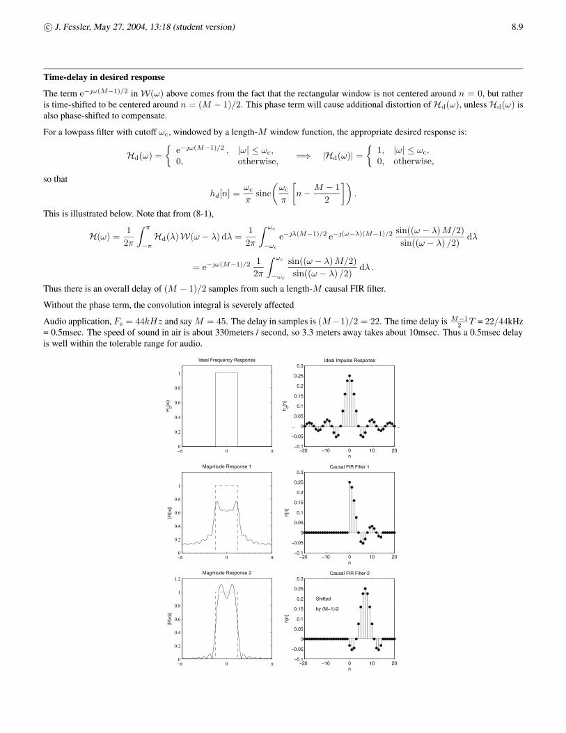
Time-delay in desired response

The term e−ω(M−1)/2 in W(ω) above comes from the fact that the rectangular window is not centered around n = 0, but ratheris time-shifted to be centered around n = (M − 1)/2. This phase term will cause additional distortion of Hd(ω), unless Hd(ω) isalso phase-shifted to compensate.

For a lowpass filter with cutoff ωc, windowed by a length-M window function, the appropriate desired response is:

Hd(ω) =

{

e−ω(M−1)/2 , |ω| ≤ ωc,0, otherwise,

=⇒ |Hd(ω)| =

{

1, |ω| ≤ ωc,0, otherwise,

so that

hd[n] =ωc

πsinc

(

ωc

π

[

n −M − 1

2

])

.

This is illustrated below. Note that from (8-1),

H(ω) =1

2π

∫ π

−π

Hd(λ)W(ω − λ) dλ =1

2π

∫ ωc

−ωc

e−λ(M−1)/2 e−(ω−λ)(M−1)/2 sin((ω − λ)M/2)

sin((ω − λ) /2)dλ

= e−ω(M−1)/2 1

2π

∫ ωc

−ωc

sin((ω − λ) M/2)

sin((ω − λ) /2)dλ .

Thus there is an overall delay of (M − 1)/2 samples from such a length-M causal FIR filter.

Without the phase term, the convolution integral is severely affected

Audio application, Fs = 44kHz and say M = 45. The delay in samples is (M−1)/2 = 22. The time delay is M−12 T = 22/44kHz

= 0.5msec. The speed of sound in air is about 330meters / second, so 3.3 meters away takes about 10msec. Thus a 0.5msec delayis well within the tolerable range for audio.

−π 0 π0

0.2

0.4

0.6

0.8

1

Ideal Frequency Response

Hd(ω

)

−20 −10 0 10 20−0.1

−0.05

0

0.05

0.1

0.15

0.2

0.25

0.3

n

h d[n]

Ideal Impulse Response

......

−20 −10 0 10 20−0.1

−0.05

0

0.05

0.1

0.15

0.2

0.25

0.3

n

h[n]

Causal FIR Filter 1

−π 0 π0

0.2

0.4

0.6

0.8

1

Magnitude Response 1

|H(ω

)|

−20 −10 0 10 20−0.1

−0.05

0

0.05

0.1

0.15

0.2

0.25

0.3

n

h[n]

Causal FIR Filter 2

Shifted

by (M−1)/2

−π 0 π0

0.2

0.4

0.6

0.8

1

1.2

|H(ω

)|

Magnitude Response 2


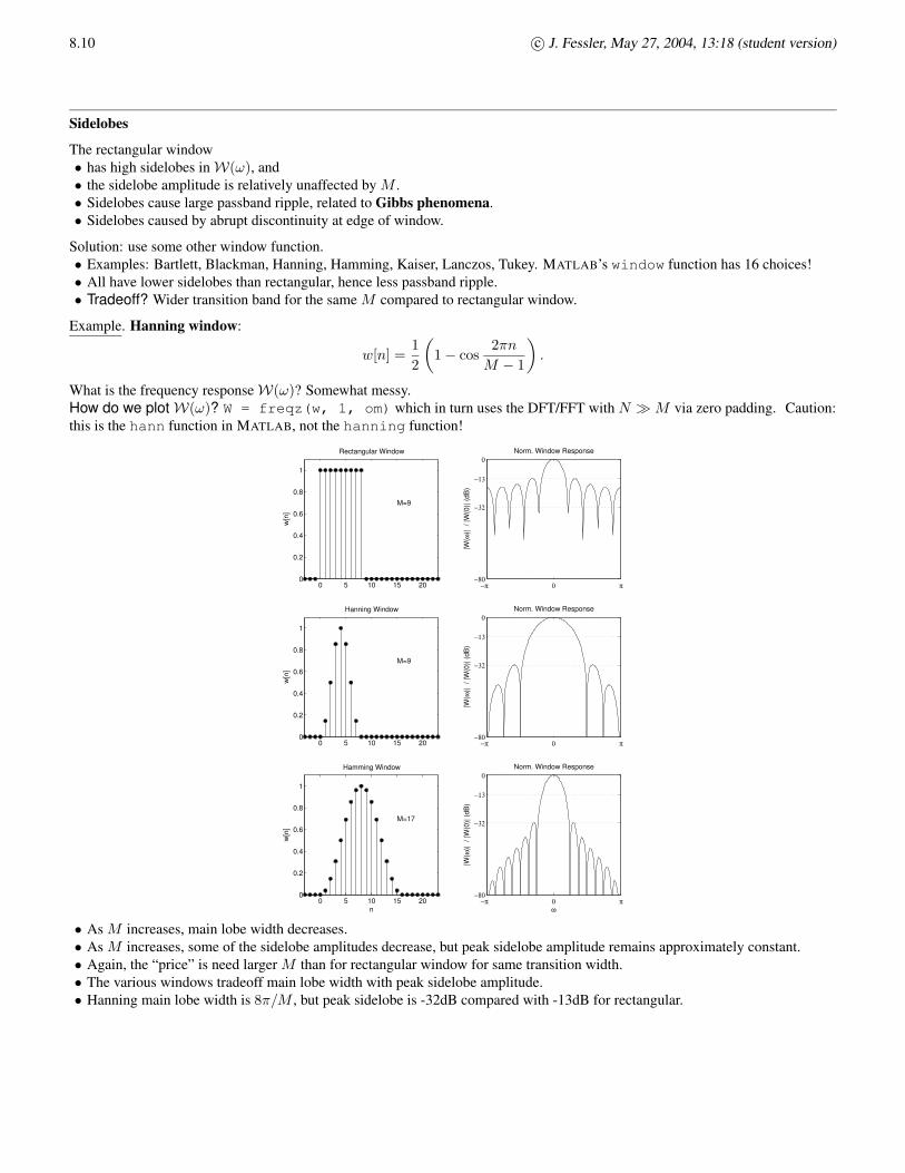
Sidelobes

The rectangular window• has high sidelobes in W(ω), and• the sidelobe amplitude is relatively unaffected by M .• Sidelobes cause large passband ripple, related to Gibbs phenomena.• Sidelobes caused by abrupt discontinuity at edge of window.

Solution: use some other window function.• Examples: Bartlett, Blackman, Hanning, Hamming, Kaiser, Lanczos, Tukey. MATLAB’s window function has 16 choices!• All have lower sidelobes than rectangular, hence less passband ripple.• Tradeoff? Wider transition band for the same M compared to rectangular window.

Example. Hanning window:

w[n] =1

2

(

1 − cos2πn

M − 1

)

.

What is the frequency response W(ω)? Somewhat messy.How do we plot W(ω)? W = freqz(w, 1, om) which in turn uses the DFT/FFT with N � M via zero padding. Caution:this is the hann function in MATLAB, not the hanning function!

0 5 10 15 200

0.2

0.4

0.6

0.8

1

w[n

]

Rectangular Window

M=9

−π 0 π−80

−32

−13

0|W

(ω)|

/ |W

(0)|

(dB

)

Norm. Window Response

0 5 10 15 200

0.2

0.4

0.6

0.8

1

w[n

]

Hanning Window

M=9

−π 0 π−80

−32

−13

0

|W(ω

)| /

|W(0

)| (d

B)


0 5 10 15 200

0.2

0.4

0.6

0.8

1

n

w[n

]

Hamming Window

M=17

−π 0 π−80

−32

−13

0

|W(ω

)| /

|W(0

)| (d

B)


ω

• As M increases, main lobe width decreases.• As M increases, some of the sidelobe amplitudes decrease, but peak sidelobe amplitude remains approximately constant.• Again, the “price” is need larger M than for rectangular window for same transition width.• The various windows tradeoff main lobe width with peak sidelobe amplitude.• Hanning main lobe width is 8π/M , but peak sidelobe is -32dB compared with -13dB for rectangular.


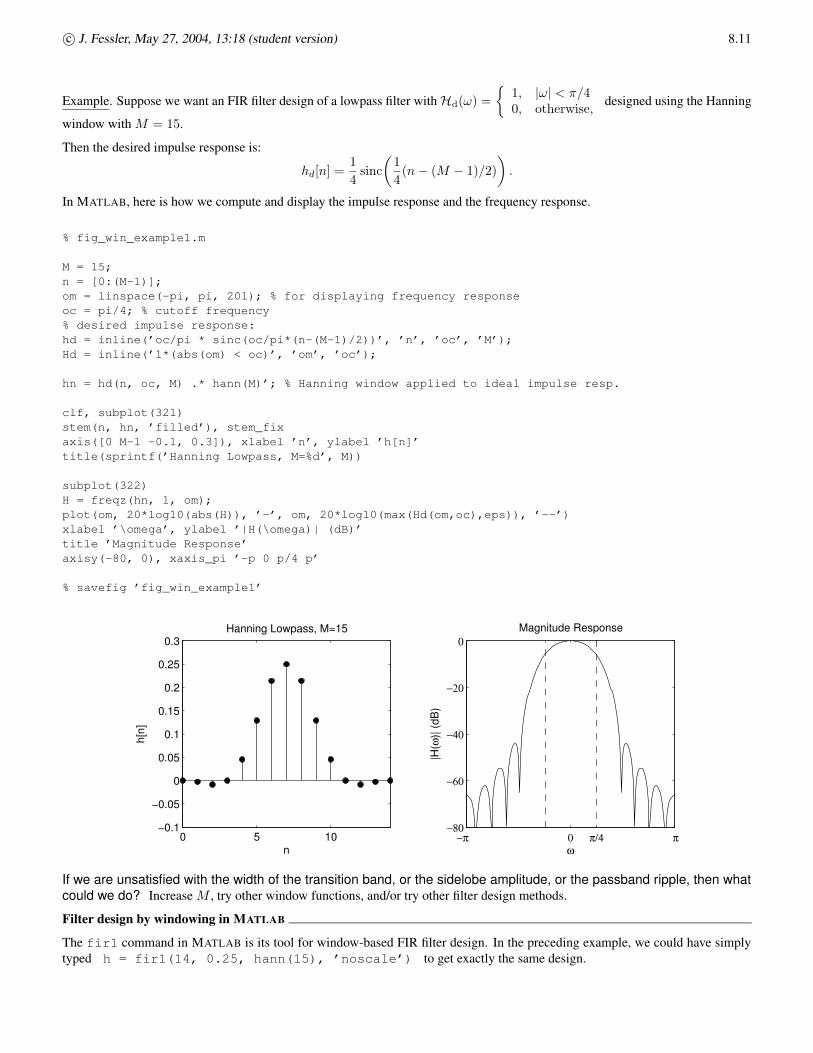
Example. Suppose we want an FIR filter design of a lowpass filter with Hd(ω) =

{

1, |ω| < π/40, otherwise,

designed using the Hanning

window with M = 15.

Then the desired impulse response is:

hd[n] =1

4sinc

(

1

4(n − (M − 1)/2)

)

.

In MATLAB, here is how we compute and display the impulse response and the frequency response.

% fig_win_example1.m

M = 15;n = [0:(M-1)];om = linspace(-pi, pi, 201); % for displaying frequency responseoc = pi/4; % cutoff frequency% desired impulse response:hd = inline(’oc/pi * sinc(oc/pi*(n-(M-1)/2))’, ’n’, ’oc’, ’M’);Hd = inline(’1*(abs(om) < oc)’, ’om’, ’oc’);

hn = hd(n, oc, M) .* hann(M)’; % Hanning window applied to ideal impulse resp.

clf, subplot(321)stem(n, hn, ’filled’), stem_fixaxis([0 M-1 -0.1, 0.3]), xlabel ’n’, ylabel ’h[n]’title(sprintf(’Hanning Lowpass, M=%d’, M))

subplot(322)H = freqz(hn, 1, om);plot(om, 20*log10(abs(H)), ’-’, om, 20*log10(max(Hd(om,oc),eps)), ’--’)xlabel ’\omega’, ylabel ’|H(\omega)| (dB)’title ’Magnitude Response’axisy(-80, 0), xaxis_pi ’-p 0 p/4 p’

% savefig ’fig_win_example1’

0 5 10−0.1

−0.05

0

0.05

0.1

0.15

0.2

0.25

0.3

n

h[n]

Hanning Lowpass, M=15

−π 0 π/4 π−80

−60

−40

−20

0

ω

|H(ω

)| (d

B)

Magnitude Response

If we are unsatisfied with the width of the transition band, or the sidelobe amplitude, or the passband ripple, then whatcould we do? Increase M , try other window functions, and/or try other filter design methods.

Filter design by windowing in MATLAB

The fir1 command in MATLAB is its tool for window-based FIR filter design. In the preceding example, we could have simplytyped h = fir1(14, 0.25, hann(15), ’noscale’) to get exactly the same design.


Example. Digital phaser or flange.

Time varying pole locations in cascade of 1st and 2nd-order allpass filters, Sum output of allpass cascade with original signal,creating time-varying notches.

8.2.5 FIR differentiator

Hd(ω) = ω

skim

8.2.6Hilbert transform (90◦ phase shift)

Hd(ω) = − sgn(ω)skip

8.2.3Design of FIR filters by frequency sampling

For the frequency sampling method of FIR filter design, to design a M -point FIR filter we specify the desired frequency responseat a set of equally-spaced frequency locations:

Hd(ω)∣

∣

∣

ω= 2πM k

, k = 0, . . . ,M − 1.

In other words, we provide equally spaced samples over [0, 2π). Picture

Recall from the DTFT formula that if hd[n] is nonzero only for n = 0, . . . ,M − 1, then

Hd(ω) =M−1∑

n=0

hd[n] e−ωn .

Thus, at the given frequency locations, we have

Hd

(

2π

Mk

)

=

M−1∑

n=0

hd[n] e− 2πM kn , k = 0, . . . ,M − 1.

This is the formula for the M -point DFT discussed in Ch. 5 (and in EECS 206).So we can determine hd[n] from

{

Hd

(

2πM k

)}M−1

k=0by using the inverse DFT formula (or h = ifft(H) in MATLAB):

hd[n] =1

M

M−1∑

k=0

Hd

(

2π

Mk

)

e 2πM kn .

This will be the impulse response of the FIR filter as designed by the frequency sampling method.• If we want hd[n] to be real, then Hd(ω) must be Hermitian symmetric, i.e., H∗

d(ω) = Hd(−ω) = Hd(2π − ω) . So if wespecify Hd

(

2πM k

)

to be some value, we know that H∗d

(

2πM k

)

= Hd

(

2π − 2πM k

)

= Hd

(

2πM (M − k)

)

, so Hd

(

2πM (M − k)

)

isalso specified.

• Thus, software such as MATLAB’s fir2 command only requires Hd(ω) only on the interval [0, π].• If hd[n] is to be real, then it also follows that Hd(π) = Hd

(

2πM

M2

)

must be real valued when M is even.• If you choose Hd(ω) to be linear phase, then the designed h[n] will be linear phase.

But you are not required to choose Hd(ω) to be linear phase!• The book discusses many further details, but the above big picture is sufficient for this class.


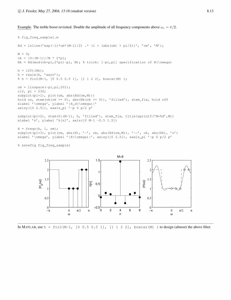
Example. The treble boost revisited. Double the amplitude of all frequency components above ωc = π/2.

% fig_freq_sample1.m

Hd = inline(’exp(-1i*om*(M-1)/2) .* (1 + (abs(om) > pi/2))’, ’om’, ’M’);

M = 9;ok = [0:(M-1)]/M * 2*pi;Hk = Hd(mod(ok+pi,2*pi)-pi, M); % trick: [-pi,pi] specification of H(\omega)

h = ifft(Hk);h = reale(h, ’warn’);% h = fir2(M-1, [0 0.5 0.5 1], [1 1 2 2], boxcar(M) );

om = linspace(-pi,pi,201);clf, pl = 230;subplot(pl+1), plot(om, abs(Hd(om,M)))hold on, stem(ok(ok >= 0), abs(Hk(ok >= 0)), ’filled’), stem_fix, hold offxlabel ’\omega’, ylabel ’|H_d(\omega)|’axisy([0 2.5]), xaxis_pi ’-p 0 p/2 p’

subplot(pl+2), stem(0:(M-1), h, ’filled’), stem_fix, title(sprintf(’M=%d’,M))xlabel ’n’, ylabel ’h[n]’, axis([0 M-1 -0.5 1.5])

H = freqz(h, 1, om);subplot(pl+3), plot(om, abs(H), ’-’, om, abs(Hd(om,M)), ’--’, ok, abs(Hk), ’o’)xlabel ’\omega’, ylabel ’|H(\omega)|’, axisy([0 2.5]), xaxis_pi ’-p 0 p/2 p’

% savefig fig_freq_sample1

−π 0 π/2 π0

0.5

1

1.5

2

2.5

ω

|Hd(ω

)|

0 2 4 6 8−0.5

0

0.5

1

1.5

n

h[n]

M=9

−π 0 π/2 π0

0.5

1

1.5

2

2.5

ω

|H(ω

)|

In MATLAB, use h = fir2(M-1, [0 0.5 0.5 1], [1 1 2 2], boxcar(M) ) to design (almost) the above filter.


8.2.4“Optimum” equiripple linear-phase FIR filters

The window method has a minor disadvantage, that it is difficult to precisely specify ωp and ωs, since these two result from thesmearing. All we really specify is ωc, the cutoff.

An “ideal” linear-phase design procedure would be as follows.

Specify ωp, ωs, δ1, δ2, and run an algorithm that returns the minimum M that achieves that design goal, as well as theimpulse response h[n], n = 0, . . . ,M − 1, where, for linear phase, h[n] = h[M − 1 − n] .

To my knowledge, there is no such procedure that is guaranteed to do this perfectly. However, we can come close using thefollowing iterative procedure.• Choose M , and find the linear-phase h[n] whose frequency response is as “close” to Hd(ω) as possible.• If it is not close enough, then increase M and repeat.

How can we measure “closeness” of two frequency response functions? Pictures of Hd(ω) and H(ω).Possible options include the following.• 1

2π

∫ π

−π|Hd(ω)−H(ω)| dω, average absolute error

• 12π

∫ π

−π|Hd(ω)−H(ω)|

2dω, average squared error

• 12π

∫ π


2W(ω) dω, average weighted squared error

•[

12π

∫ π


pW(ω) dω

]1/p

, weighted Lp error, p ≥ 1

• maxω |Hd(ω)−H(ω)|, maximum error (p = ∞)• maxω |W(Hd(ω)−H(ω))|, maximum weighted error (p = ∞)

In this section, we focus on the last choice, the maximum weighted error between the desired response and the actual frequencyresponse of an FIR filter. We want to find the FIR filter that minimizes this error.How to find this? Not by brute force search or trial and error, but by analysis!

If W(ω) ≥ 0 then

E(ω)4= |W(Hd(ω)−H(ω))| = W(ω) |Hd(ω)−H(ω)| .

Consider the case of a lowpass filter. Note that

Hd(ω) =

{

e−ω(M−1)/2 , |ω| ≤ ωc,0, |ω| > ωc

= e−ω(M−1)/2 Hdr(ω) where Hdr(ω) =

{

1, |ω| ≤ ωc,0, |ω| > ωc.

Also recall that for M even and h[n] linear phase and symmetric,

H(ω) = e−ω(M−1)/2 Hr(ω), where Hr(ω) =

M/2−1∑

n=0

h[n] 2 cos

(

ω

(

M − 1

2− n

))

.

So Hr(ω) is the sum of M/2 cosines.

The error can be simplified as follows:

E(ω) = W(ω) |Hd(ω)−H(ω)|

= W(ω)∣

∣

∣e−ω(M−1)/2 Hdr(ω)− e−ω(M−1)/2 Hr(ω)

∣

∣

∣

= W(ω) |Hdr(ω)−Hr(ω)| .

Thus we only need to consider the “real” parts of the desired vs actual frequency response.


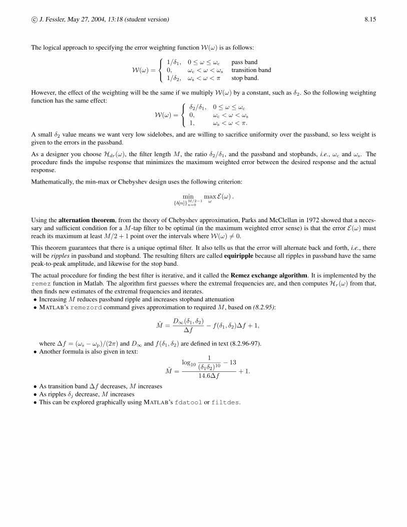
The logical approach to specifying the error weighting function W(ω) is as follows:

W(ω) =

1/δ1, 0 ≤ ω ≤ ωc pass band0, ωc < ω < ωs transition band1/δ2, ωs < ω < π stop band.

However, the effect of the weighting will be the same if we multiply W(ω) by a constant, such as δ2. So the following weightingfunction has the same effect:

W(ω) =

δ2/δ1, 0 ≤ ω ≤ ωc

0, ωc < ω < ωs

1, ωs < ω < π.

A small δ2 value means we want very low sidelobes, and are willing to sacrifice uniformity over the passband, so less weight isgiven to the errors in the passband.

As a designer you choose Hdr(ω), the filter length M , the ratio δ2/δ1, and the passband and stopbands, i.e., ωc and ωs. Theprocedure finds the impulse response that minimizes the maximum weighted error between the desired response and the actualresponse.

Mathematically, the min-max or Chebyshev design uses the following criterion:

min{h[n]}

M/2−1

n=0

maxω

E(ω) .

Using the alternation theorem, from the theory of Chebyshev approximation, Parks and McClellan in 1972 showed that a neces-sary and sufficient condition for a M -tap filter to be optimal (in the maximum weighted error sense) is that the error E(ω) mustreach its maximum at least M/2 + 1 point over the intervals where W(ω) 6= 0.

This theorem guarantees that there is a unique optimal filter. It also tells us that the error will alternate back and forth, i.e., therewill be ripples in passband and stopband. The resulting filters are called equiripple because all ripples in passband have the samepeak-to-peak amplitude, and likewise for the stop band.

The actual procedure for finding the best filter is iterative, and it called the Remez exchange algorithm. It is implemented by theremez function in Matlab. The algorithm first guesses where the extremal frequencies are, and then computes Hr(ω) from that,then finds new estimates of the extremal frequencies and iterates.• Increasing M reduces passband ripple and increases stopband attenuation• MATLAB’s remezord command gives approximation to required M , based on (8.2.95):

M̂ =D∞(δ1, δ2)

∆f− f(δ1, δ2)∆f + 1,

where ∆f = (ωs − ωp)/(2π) and D∞ and f(δ1, δ2) are defined in text (8.2.96-97).• Another formula is also given in text:

M̂ =

log10

1

(δ1δ2)10− 13

14.6∆f+ 1.

• As transition band ∆f decreases, M increases• As ripples δj decrease, M increases• This can be explored graphically using MATLAB’s fdatool or filtdes.


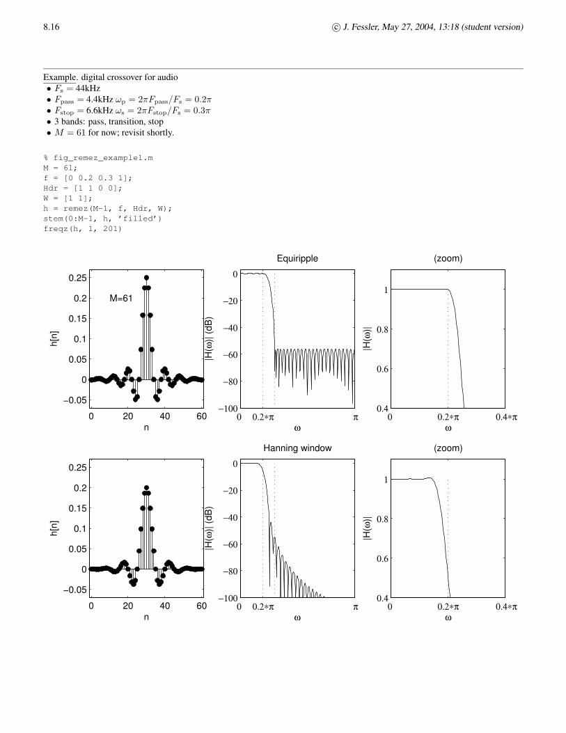
Example. digital crossover for audio• Fs = 44kHz• Fpass = 4.4kHz ωp = 2πFpass/Fs = 0.2π• Fstop = 6.6kHz ωs = 2πFstop/Fs = 0.3π• 3 bands: pass, transition, stop• M = 61 for now; revisit shortly.

% fig_remez_example1.mM = 61;f = [0 0.2 0.3 1];Hdr = [1 1 0 0];W = [1 1];h = remez(M-1, f, Hdr, W);stem(0:M-1, h, ’filled’)freqz(h, 1, 201)

0 20 40 60

−0.05

0

0.05

0.1

0.15

0.2

0.25

n

h[n]

M=61

0 0.2∗π π−100

−80

−60

−40

−20

0

ω

|H(ω

)| (d

B)

Equiripple

0 0.2∗π 0.4∗π0.4

0.6

0.8

1

ω

|H(ω

)|

(zoom)

0 20 40 60

−0.05

0

0.05

0.1

0.15

0.2

0.25

n

h[n]

0 0.2∗π π−100

−80

−60

−40

−20

0

ω

|H(ω

)| (d

B)

Hanning window

0 0.2∗π 0.4∗π0.4

0.6

0.8

1

ω

|H(ω

)|

(zoom)


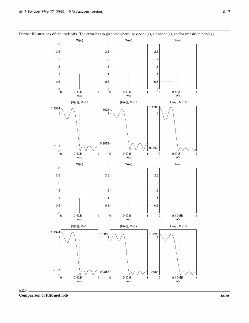
Further illustrations of the tradeoffs. The error has to go somewhere: passband(s), stopband(s), and/or transition band(s).

0 0.40.5 10

0.5

1

1.5

2

2.5

3

ω/π

W(ω)

0 0.40.5 10

0.137

1

1.1374

ω/π

|H(ω)|, M=13

0 0.40.5 10

0.5

1

1.5

2

2.5

3

ω/π

W(ω)

0 0.40.5 10

0.2053

11.1026

ω/π

|H(ω)|, M=13

0 0.40.5 10

0.5

1

1.5

2

2.5

3

ω/π

W(ω)

0 0.40.5 10

0.0859

1

1.1708

ω/π

|H(ω)|, M=13

0 0.40.5 10

0.5

1

1.5

2

2.5

3

ω/π

W(ω)

0 0.40.5 10

0.137

1

1.1374

ω/π

|H(ω)|, M=13

0 0.40.5 10

0.5

1

1.5

2

2.5

3

ω/π

W(ω)

0 0.40.5 10

0.0857

11.0858

ω/π

|H(ω)|, M=17

0 0.4 0.55 10

0.5

1

1.5

2

2.5

3

ω/π

W(ω)

0 0.4 0.55 10

0.084

11.0838

ω/π

|H(ω)|, M=13

8.2.7Comparison of FIR methods skim


8.3Design of IIR Filters from Analog Filters

Why IIR? With IIR designs we can get the same approximation accuracy (of the magnitude response) as FIR but with a lower orderfilter. The tradeoff is nonlinear phase.

Analog filter design is a mature field. There are well known methods for selecting RLC combinations to approximate some desiredfrequency response Hd(F ).

Generally, the more (passive) components used, the closer one can approximate Hd(F ), (to within component tolerances).

Essentially all analog filters are IIR, since the solutions to linear differential equations involve infinite-duration terms of the formtm eλt u(t).

One way to design IIR digital filters is to piggyback on this wealth of design experience for analog filters.

What do analog filters look like?

Any RLC network is describe by a linear constant coefficient differential equation of the form

N∑

k=0

αkdk

dtkya(t) =

M∑

k=0

βkdk

dtkxa(t)

with corresponding system function (Laplace transform of the impulse response)

Ha(s) =

∑Mk=0 βksk

∑Nk=0 αksk

.

Each combination of N,M, {αk} , {βk} corresponds to some arrangement of RLCs. Those implementation details are unimportantto us here.

The frequency response of a general analog filter is

Ha(F ) = Ha(s)∣

∣

∣

s=2πF.

Overview• Design N,M, {αk} , {βk} using existing methods.• Map from s plane to z-plane somehow to get ak’s and bk’s, i.e., a rational system function corresponding to a discrete-time

linear constant coefficient difference equation.

Can we achieve linear phase with an IIR filter? We should be able to use our analysis tools to answer this.

Recall that linear phase implies thatH(z) = z−N H

(

z−1)

,

so if z is a pole of the system function H(z), then z−1 is also a pole. So any finite poles (i.e., other than 0 or ∞) would lead toinstability.

There are no causal stable IIR filters with linear phase.

Thus we design for the magnitude response, and see what phase response we get.

8.3.1 IIR by approximation of derivatives skim

s =1 − z−1

T

8.3.2 IIR by impulse invariance skimh[n] = ha(nT )

z = esT


8.3.3IIR filter design by bilinear transformation

Suppose we have used existing analog filter design methods to design an IIR analog filter with system function

Ha(s) =

∑Mk=0 βksk

∑Nk=0 αksk

.

For a sampling period Ts, we now make the bilinear transformation

s =2

Ts

1 − z−1

1 + z−1.

This transformation can be motivated by the trapezoidal formula for numerical integration. See text for the derivation.

Define the discrete-time system function

H(z) = Ha(s)∣

∣

∣

s=2

Ts

1 − z−1

1 + z−1

.

This transformation yields a rational system function, i.e., a ratio of polynomials in z.

This H(z) is a system function whose frequency response is related to the frequency response of the analog IIR filter.

Example. Consider a 1st-order analog filter with a single pole at s = −α Picture where α > 0, with system function

Ha(s) =1

α + s.

How would you build this? Using the following RL “voltage divider,” where Vout(s) = RR+sLVin(s) =⇒ Ha(s) = R/L

R/L+s .

+

−

i(t)

vin(t)

L

R vout(t)

Applying the bilinear transformation to the above (Laplace domain) system function yields:

H(z) = Ha(s)∣

∣

∣

s=2

Ts

1 − z−1

1 + z−1

=1

α +2

Ts

1 − z−1

1 + z−1

=1 + z−1

α(1 + z−1) +2

Ts(1 − z−1)

=1 + z−1

(α + 2/Ts) + (α − 2/Ts)z−1

=1

α + 2/Ts

1 + z−1

1 −2/Ts − α

2/Ts + αz−1

=1

α + 2/Ts

1 + z−1

1 − pz−1=

1

α + 2/Ts

[

−1

p+

1 + 1/p

1 − pz−1

]

,

where p =2 − αTs

2 + αTs∈ (−1, 1). What is h[n]? h[n] = 1

α+2/Ts

(

− 1p δ[n] +(1 + 1/p)pn u[n]

)

.

Re(z)

Im(z)

p

Where did zero at z = −1 come from?


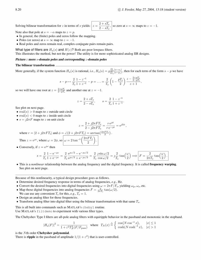
Solving bilinear transformation for z in terms of s yields: z =2 + sTs

2 − sTs, so zero at s = ∞ maps to z = −1.

Note also that pole at s = −α maps to z = p.• In general, the (finite) poles and zeros follow the mapping.• Poles (or zeros) at s = ∞ map to z = −1.• Real poles and zeros remain real, complex-conjugate pairs remain pairs.

What type of filters are Ha(s) and H(z)? Both are poor lowpass filters.This illustrates the method, but not the power! The utility is for more sophisticated analog IIR designs.

Picture : more s-domain poles and corresponding z-domain poles

The bilinear transformation

More generally, if the system function Ha(s) is rational, i.e., Ha(s) = g∏

i(s−si)∏

j(s−pj), then for each term of the form s − p we have

s − p 7→2

Ts

1 − z−1

1 + z−1− p = . . . =

2

Ts

(

1 −pTs

2

)

z − 2+pTs

2−pTs

z + 1,

so we will have one root at z = 2+pTs

2−pTs

and another one at z = −1.

z =2 + sTs

2 − sTs, s =

2

Ts

1 − z−1

1 + z−1.

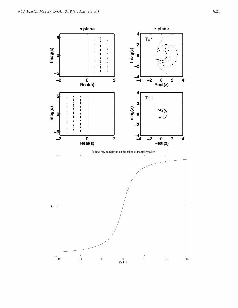
See plot on next page.• real(s) > 0 maps to z outside unit circle• real(s) < 0 maps to z inside unit circle• s = 2πF maps to z on unit circle

z =2 + 2πFTs

2 − 2πFTs=

r eφ

r e−φ= e2φ ,

where r = |2 + 2πFTs| and φ = ∠(2 + 2πFTs) = arctan(

2πFTs

2

)

.

Thus z = eω , where ω = 2φ, so ω = 2 tan−1

(

2πFTs

2

)

.

• Conversely, if z = eω then

s =2

Ts

1 − e−ω

1 + e−ω=

2

Ts

eω/2 − e−ω/2

eω/2 + e−ω/2=

2

Ts

sin ω/2

cosω/2=

2

Tstan

(ω

2

)

=⇒ F =2

2πTstan

(ω

2

)

.

• This is a nonlinear relationship between the analog frequency and the digital frequency. It is called frequency warping.See plot on next page.

Because of this nonlinearity, a typical design procedure goes as follows.• Determine desired frequency response in terms of analog frequencies, e.g., Hz.• Convert the desired frequencies into digital frequencies using ω = 2πF/Fs, yielding ωp, ωs, etc.• Map those digital frequencies into analog frequencies F = 2

2πTs

tan(ω/2).We can use any convenient Ts for this, e.g., Ts = 1.

• Design an analog filter for those frequencies.• Transform analog filter into digital filter using the bilinear transformation with that same Ts.

This is all built into commands such as MATLAB’s cheby1 routine.Use MATLAB’s filtdemo to experiment with various filter types.

The Chebyshev Type I filters are all-pole analog filters with equiripple behavior in the passband and monotonic in the stopband.

|Ha(F )|2

=1

1 + ε2T 2N (F/Fpass)

where TN (x)4=

{

cos(

N cos−1 x)

, |x| ≤ 1

cosh(N cosh−1 x), |x| > 1

is the N th order Chebyshev polynomial.There is ripple in the passband of amplitude 1/(1 + ε2) that is user-controlled.


−2 0 2

−5

0

5

Real(s)

Imag

(s)

s plane

−4 −2 0 2 4−4

−2

0

2

4

Real(z)

Imag

(z)

T=1

z plane

−2 0 2

−5

0

5

Real(s)

Imag

(s)

−4 −2 0 2 4−4

−2

0

2

4

Real(z)

Imag

(z)

T=1

−15 −10 −5 0 5 10 15−π

0

π

2π F T

ω

Frequency relationships for bilinear transformation


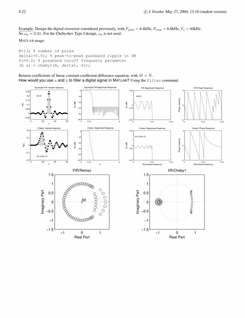
Example. Design the digital crossover considered previously, with Fpass = 4.4kHz, Fstop = 6.6kHz, Fs = 44kHz.So ωp = 0.2π. For the Chebyshev Type I design, ωp is not used.

MATLAB usage:

N=13; % number of polesdelta1=0.01; % peak-to-peak passband ripple in dBfc=0.2; % passband cutoff frequency parameter[b a] = cheby1(N, delta1, fc);

Returns coefficients of linear constant coefficient difference equation, with M = N .How would you use a and b to filter a digital signal in MATLAB? Using the filter command.

0 20 40 60

−0.05

0

0.05

0.1

0.15

0.2

0.25

n

h[n]

Equiripple FIR impulse response

M=61

0 0.2π π−100

−80

−60

−40

−20

0

|H| (

dB)

Equiripple FIR Magnitude Response

0 20 40 60−0.2

−0.1

0

0.1

0.2

n

h[n]

Cheby1 impulse response

N=13 M=13

0 0.2π π−100

−80

−60

−40

−20

0

ω

|H| (

dB)

Cheby1 Magnitude Response

0 0.2π 0.4π−0.05

−0.010

0.05FIR Magnitude Response

|H| (

dB)

M=61

0 0.2π 0.4π−0.05

−0.010

0.05Cheby1 Magnitude Response

Normalized frequency

|H| (

dB)

N=13 M=13

0 0.2π 0.4π−π

0

π

Pha

se (r

adia

ns)

FIR Phase Response

0 0.2π 0.4π−π

0

π

Normalized frequency

Pha

se (r

adia

ns)

Cheby1 Phase Response

−1 0 1−1.5

−1

−0.5

0

0.5

1

1.5

60

Real Part

Imag

inar

y P

art

FIR/Remez

−1 0 1−1.5

−1

−0.5

0

0.5

1

1.5

Real Part

Imag

inar

y P

art

IIR/Cheby1


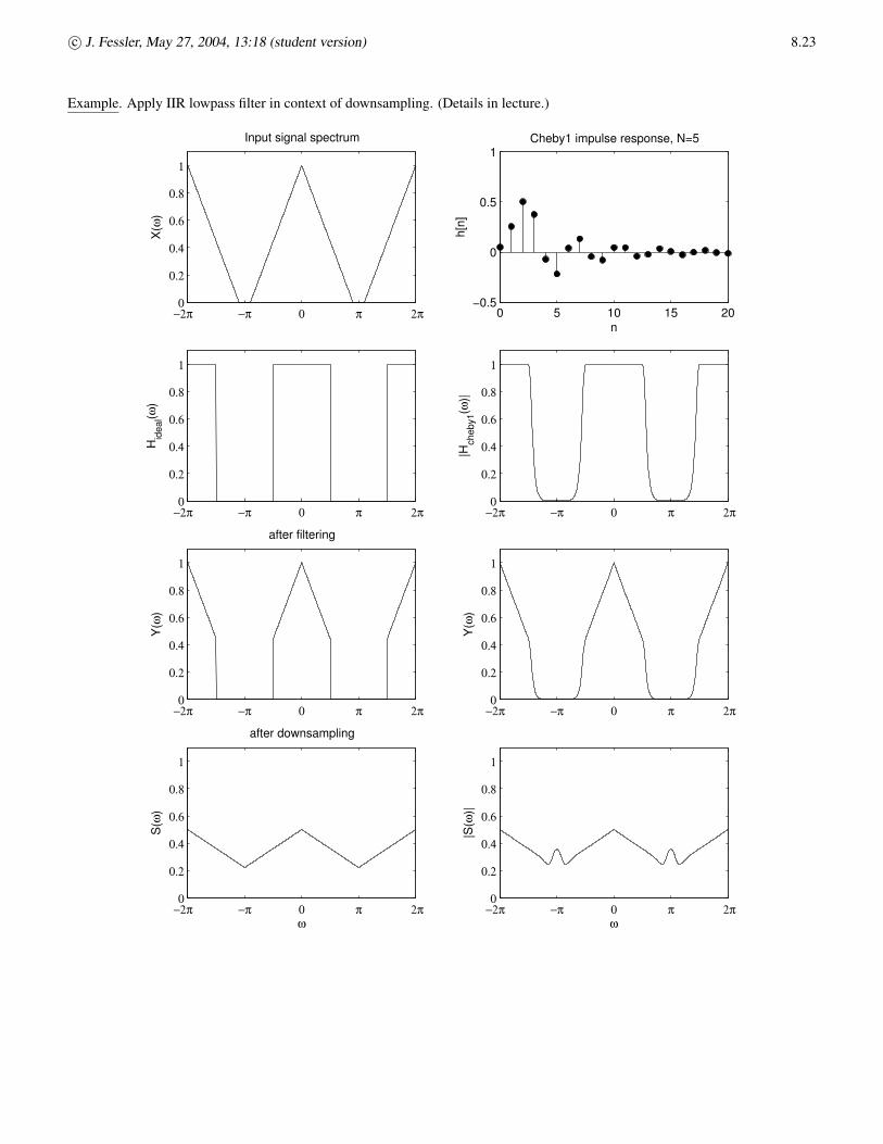
Example. Apply IIR lowpass filter in context of downsampling. (Details in lecture.)

−2π −π 0 π 2π0

0.2

0.4

0.6

0.8

1

Input signal spectrumX

(ω)

−2π −π 0 π 2π0

0.2

0.4

0.6

0.8

1

Hid

eal(ω

)

−2π −π 0 π 2π0

0.2

0.4

0.6

0.8

1

after filtering

Y(ω

)

−2π −π 0 π 2π0

0.2

0.4

0.6

0.8

1

after downsampling

ω

S(ω

)

0 5 10 15 20−0.5

0

0.5

1

n

h[n]

Cheby1 impulse response, N=5

−2π −π 0 π 2π0

0.2

0.4

0.6

0.8

1

|Hch

eby1

(ω)|

−2π −π 0 π 2π0

0.2

0.4

0.6

0.8

1

Y(ω

)

−2π −π 0 π 2π0

0.2

0.4

0.6

0.8

1

ω

|S(ω

)|


8.4Frequency Transformations

skim

Convert lowpass to highpass, bandpass, etc.

8.5Design of Digital Filters Based on Least-Squares Method

skim

8.6Summary• FIR can provide exactly linear phase• IIR can provide similar magnitude response with fewer coefficients, or lower sidelobes for same number of coefficients• FIR designs by windowed sinc or frequency sampling are simple• FIR equiripple designs allow better control of frequency breakpoints and of passband and stopband ripple.

it is more complicated to implement, but that was solved 30 years ago...• IIR can be designed by mapping analog filter to digital. The bilinear transformation is particularly flexible, but frequency

warping must be taken into account.• more coefficients: closer to desired response• wider transition band: less ripple in passband, more stopband attenuation

Summary of tradeoffs

FIR• + linear phase if symmetric: h[n] = h[N − 1 − n], n = 0, . . . , N − 1• + easy to design (especially windowed FIR)

IIR• - never exactly linear phase• + comparable (or even better!) magnitude response as FIR but with lower order (using poles and zeros)

Windowed FIR

Larger M (vs smaller M )• + |H(ω)| better approximation to Hd(ω)• + Sharper transition band• + some sidelobes have reduced amplitude• - peak sidelobe in stopband relatively unaffected• - more computation (or more hardware)• - longer delay

Nonrectangular windows (vs rectangular window)• + lower sidelobe amplitude• + less passband ripple• - wider transition band

design of digital filters

Documents