design of smart composite materials using topology...
TRANSCRIPT

Smart Mater. Struct.8 (1999) 365–379. Printed in the UK PII: S0964-1726(99)02176-X
Design of smart composite materialsusing topology optimization
O Sigmund † and S Torquato ‡
† Department of Solid Mechanics, Technical University of Denmark, DK-2800 Lyngby,Denmark‡ Department of Civil Engineering and Operations Research and Princeton MaterialsInstitute, Princeton University, Princeton, NJ 08544, USA
Received 2 December 1997, in final form 2 November 1998
Abstract. The topology optimization method is used to find the distribution of materialphases that extremizes an objective function (e.g., thermal expansion coefficient, piezoelectriccoefficients etc) subject to constraints, such as elastic symmetry and volume fractions of theconstituent phases, within a periodic base cell. The effective properties of the materialstructures are found using a numerical homogenization method based on a finite-elementdiscretization of the base cell. The optimization problem is solved using sequential linearprogramming. We review the topology optimization procedure as a tool for smart materialsdesign and discuss in detail two recent applications of it to design composites with extremethermal expansion coefficients and piezocomposites with optimal hydrophone characteristics.
1. Introduction
Smart material systems often consist of mixtures of severaldifferent passive and active materials. Mixing the constituentmaterials in the right way makes it possible to make new smartcomposites with properties beyond those of the individualconstituents. Whereas the modeling of composite materialsconsisting of various passive and active materials has beenstudied in detail in numerous research papers, only a fewpapers have considered the systematic design or synthesis ofsmart materials.
A promising new method for the systematic design ofsmart materials is thetopology optimization method. Thetopology optimization method was founded a decade ago byBendsøe and Kikuchi [1] and was originally intended for thedesign of mechanical structures. Since then, the method hasreached a level of maturity where it is being applied to manyindustrial problems. In academia it is being used not onlyto solve structural problems but also in smart and passivematerial design, mechanism design, microelectromechanicalsystems (MEMS) design and many other design problems.In the following we will introduce the topology optimizationin further detail, review its applications and discuss itsapplicability to smart materials design.
The basic form of a topology optimization problem canbe defined as follows:distribute a given amount of material ina design domain such that an objective function is extremized.A typical example would be the design of a load-bearingstructure for maximum stiffness (or minimum compliance)where the weight should be kept under a certain limit. Findingthe optimal topology corresponds to finding the optimalconnectedness, shape and number of holes in the structuresuch that the objective function is extremized.
The topology optimization problem is initialized bydiscretizing the design domain by a large number of elements.Allowing each element to be either solid or void, one canimagine that a ‘bit-map’ of the structure can be obtained byturning on or off the individual elements or pixels. This 0/1problem is ill posed since a refinement of the mesh results ina solution with finer details [2]. In fact, it can be shown thatoptimal structures (at least for compliance optimization) willconsist of regions with infinitely fine microstructure (e.g. [3]and references therein). In order to encompass composites,i.e. structures with fine microstructure, [1] introduced amicroscale through the use of the so-calledhomogenizationapproach to topology optimization. For an overview of thehomogenization approach to topology optimization and itsmathematical background, the reader is referred to [4] andreferences therein. Recently the method has been applied tothree-dimensional problems (e.g. [5, 6, 7]) and for multiplematerial problems [8]. A disadvantage of the homogenizationapproach is that it often produces structures with large ‘grey’regions consisting of perforated material. This problem canbe overcome by introducing a penalization of intermediatedensities.
An alternative to the homogenization approach is theSIMP (simple isotropic material with penalization [9])approach (see also [10, 11]). Using the SIMP approachthe stiffness tensor of an intermediate density material isCijkl(ρ) = C0
ijklρp, whereC0
ijkl is the stiffness tensor ofsolid material andp is the penalization factor which ensuresthat the continuous design variables are forced towards ablack and white (0/1) solution. The influence of the penaltyparameter can be explained as follows. By specifying a valueof p higher than one, the local stiffness forρ < 1 is lowered,thus making it ‘uneconomical’ to have intermediate densitiesin the optimal design. Even though the SIMP formulation is
0964-1726/99/030365+15$19.50 © 1999 IOP Publishing Ltd 365
O Sigmund and S Torquato
ill posed (mesh dependent), it is popular because it is easy toimplement in commercial finite element codes and becausethe simple model allows for consideration of more advancedproblems than the compliance optimization problem. A wayof achieving well posedness of the SIMP problem is byrestricting the design space by introducing a constraint on thedensity variation of the microstructure. This can be done byintroducing a perimeter constraint [12, 13, 14, 15, 16], a localgradient constraint [17] or a (heuristic) filtering approach[18, 19].
In recent work, the SIMP approach to topologyoptimization has been applied to three-dimensional problems(e.g. [20, 21]), non-linear elasticity [22], plasticity [23, 24],stress constraints [25, 26], controlled structures [27] and inMEMS design [28, 29, 19]. It should be emphasized herethat the references we have listed here by no means give anexhaustive listing of the numerous interesting applicationsof the topology optimization method which have appearedduring recent years. For more references the reader is referredto the conference literature and to [4].
An application of the topology optimization methodof special importance to smart materials design is thedesign of materials with extreme elastic properties. In thisclass of topology optimization problems, the design domainis the base cell of a periodic material and the objectivefunction is to extremize some function of the effectiveproperties. The design of material structures with extremeelastic properties is considered in [30, 18, 31, 32, 24], withextremethermoelasticproperties and three material phasesin [18, 33, 34] and applications to design ofpiezoelectriccomposites are found for two-dimensional problems in [35]and for three dimensions in [21].
In this paper, we will review the topology optimizationmethod applied to smart composite material design based onreferences [33, 34, 21].
The topology optimization procedure described hereessentially follows the steps of conventional topologyoptimization procedures based on the SIMP approach. Thedesign problem is initialized by defining a design domain (thebase cell) discretized by a number of finite elements. Theoptimization procedure then consists in solving a sequenceof finite-element problems followed by changes in densityand/or material type of each of the finite elements, dependenton the local strain energies. For simple complianceoptimization, this corresponds to adding material where thestrain energy density is high and removing material wherethe strain energy density is low.
At each step of the topology optimization procedure, wehave to determine the effective properties of the microstruc-ture. There exist several methods to determine these prop-erties. However, because the topology optimization methodis based on finite-element discretizations, and because thefinite-element method allows easy derivation and evaluationof the sensitivities of the effective properties with respectto design changes, we have chosen to use a finite-elementbased numerical homogenization procedure as developed in[36, 37].
We can use the topology procedure to design compositematerials with extreme elastic, thermal or piezoelectricproperties. In the case of elastic properties, for example, one
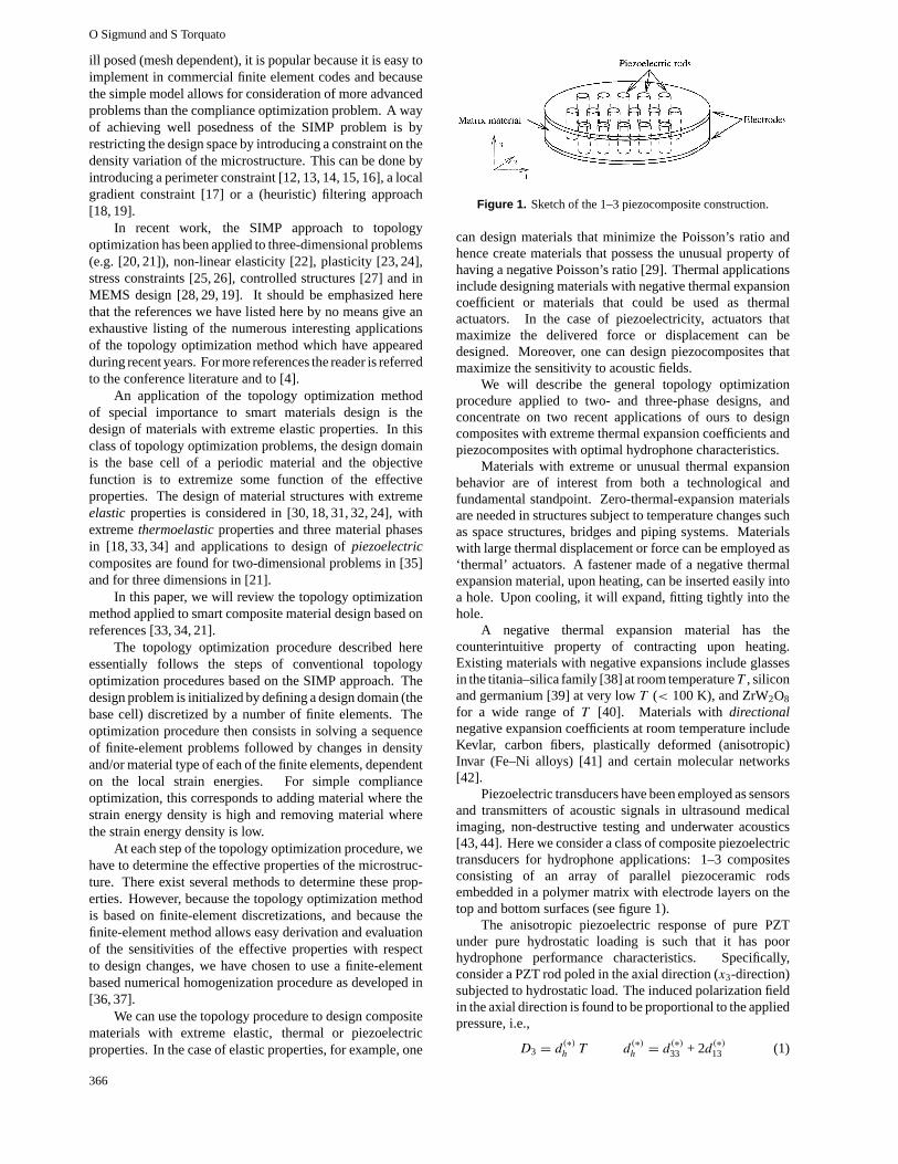
Figure 1. Sketch of the 1–3 piezocomposite construction.
can design materials that minimize the Poisson’s ratio andhence create materials that possess the unusual property ofhaving a negative Poisson’s ratio [29]. Thermal applicationsinclude designing materials with negative thermal expansioncoefficient or materials that could be used as thermalactuators. In the case of piezoelectricity, actuators thatmaximize the delivered force or displacement can bedesigned. Moreover, one can design piezocomposites thatmaximize the sensitivity to acoustic fields.
We will describe the general topology optimizationprocedure applied to two- and three-phase designs, andconcentrate on two recent applications of ours to designcomposites with extreme thermal expansion coefficients andpiezocomposites with optimal hydrophone characteristics.
Materials with extreme or unusual thermal expansionbehavior are of interest from both a technological andfundamental standpoint. Zero-thermal-expansion materialsare needed in structures subject to temperature changes suchas space structures, bridges and piping systems. Materialswith large thermal displacement or force can be employed as‘thermal’ actuators. A fastener made of a negative thermalexpansion material, upon heating, can be inserted easily intoa hole. Upon cooling, it will expand, fitting tightly into thehole.
A negative thermal expansion material has thecounterintuitive property of contracting upon heating.Existing materials with negative expansions include glassesin the titania–silica family [38] at room temperatureT , siliconand germanium [39] at very lowT (< 100 K), and ZrW2O8
for a wide range ofT [40]. Materials with directionalnegative expansion coefficients at room temperature includeKevlar, carbon fibers, plastically deformed (anisotropic)Invar (Fe–Ni alloys) [41] and certain molecular networks[42].
Piezoelectric transducers have been employed as sensorsand transmitters of acoustic signals in ultrasound medicalimaging, non-destructive testing and underwater acoustics[43, 44]. Here we consider a class of composite piezoelectrictransducers for hydrophone applications: 1–3 compositesconsisting of an array of parallel piezoceramic rodsembedded in a polymer matrix with electrode layers on thetop and bottom surfaces (see figure 1).
The anisotropic piezoelectric response of pure PZTunder pure hydrostatic loading is such that it has poorhydrophone performance characteristics. Specifically,consider a PZT rod poled in the axial direction (x3-direction)subjected to hydrostatic load. The induced polarization fieldin the axial direction is found to be proportional to the appliedpressure, i.e.,
D3 = d(∗)h T d(∗)h = d(∗)33 + 2d(∗)13 (1)
366

Topology optimization
whereD3 is the dielectric displacement in thex3-direction,T is the amplitude of the applied pressure,d(∗)h is thehydrostatic coupling coefficient andd(∗)33 and d
(∗)13 are
the longitudinal and transverse piezoelectric coefficientscharacterizing the dielectric response for axial and lateralcompression, respectively. Unfortunately,d(∗)33 and d(∗)13have opposite signs, thus resulting in a relatively smallhydrostatic coupling factord(∗)h . For instance, PZT5A hasd(∗)33 = 374 pC N−1 andd(∗)13 = −171 pC N−1. Therefore,d(∗)h = 32 pC N−1 which is small compared tod(∗)33 . As
we will see, a polymer/piezoceramic composite can have asensitivity that is orders of magnitude greater than a purepiezoceramic device. Using a piezo/polymer composite, thefactor of 2 on the transverse piezoelectric coefficientd
(∗)13
in equation (1) can be lowered, or even change sign, if weuse a soft matrix material or a matrix material with negativePoisson’s ratio (e.g. Smith [44]), thereby ensuring a muchhigher hydrostatic charge coefficient.
The remainder of the paper is organized in the followingway. In section 2 we describe the topology optimizationprocedure for two and three phases and its application todesign of material structures with extremal effective behavior.The sequential linear programming method used to solve thetopology optimization problem is described in section 2.2 andnumerical implementation issues are discussed in section 2.3.Section 3 summarizes our work on the design of compositeswith extreme thermal expansion coefficients. Section 4reviews our work on the optimal design of matrix materialsfor 1–3 piezocomposites. Finally, in section 5 we makeconcluding remarks.
2. Procedures for two- or three-phase topologyoptimization
We assume perfect bonding between the material phases andthat the behavior of materials can be described by the lineargeneralized Hooke law given as
σij = Cijklεkl − Cijklαkl1T − CijkldmklEm= Cijklεkl − βij1T − eijmEm (2)
whereCijkl , σij , εkl , αkl , βij , dijm andeijm are the elasticity,stress, strain, thermal strain, thermal stress, piezoelectricstrain and piezoelectric stress tensors, respectively, and1T
is the temperature change andEm is the electric field. Werefer toαkl as the ‘thermal strain tensor’ (the resulting strainof a material which is allowed to expand freely and whichis subjected to increase in temperature of one unit) and toβij as the ‘thermal stress tensor’ (the stress in a materialwhich is not allowed to expand and which is subjected toincrease in temperature of one unit). Equivalent definitionscan be made for the piezoelectric strain and stress tensorsdijmandeijm. For the two- or three-phase composite of interest,the constitutive equation (2) is valid on a local scale (withsuperscripts (0), (1) and (2) appended to the properties, e.g.C(m)ijkl , α
(m)ij , β(m)ij , d(m)ijm ande(m)ijm) and the macroscopic scale
(with superscript (*) appended to the properties). In the lattercase, the stresses and strains are averages over local stresses
and strains, respectively, i.e.
σ ij = C(∗)ijklεkl − C(∗)ijklα(∗)kl 1T − C(∗)ijkld(∗)mklEm= C(∗)ijklεkl − β(∗)ij 1T − e(∗)ijmEm (3)
where the overbar denotes the volume average. The effectivethermoelastic and piezoelectric properties,C
(∗)ijkl , α
(∗)kl , β(∗)ij ,
d(∗)mkl and e(∗)ijm of the composite are computed using a
numerical homogenization method as described in Sigmundand Torquato [33].
The general goal is to optimize components orcombinations of components of the effective tensors bydistributing, in a clever way, given amounts of one ortwo material phases and void within the design domainrepresenting a base cell of a periodic material. In otherwords, we want to design microstructural topologies that giveus some desirable overall thermoelastic properties. As willbe seen later, materials with extreme thermal expansion orpiezoelectric properties tend to have low overall stiffness.Thus, for practical applications, one must bound the effectivestiffness or bulk moduli from below. It should also bepossible to specify elastic symmetries such as orthotropy,square symmetry or isotropy of the resulting materials.
An optimization problem including these features can bewritten as
minimize : some effective propertyvariables : distribution of one or two material phases and
void in the base cellsubject to : constraints on volume fractions
: orthotropy, square symmetry or isotropyconstraints
: lower bound constraints on stiffness: bounds on design variables. (4)
2.1. Formulation of the optimization problem
This subsection discusses the individual parts of theoptimization problem defined in equation (4). We generallyconsiderd-dimensional composites (withd = 2 or 3)that are comprised of two or three phases. In sections 3and 4 we specialize to thermoelasticity and piezoelectricity,respectively.
2.1.1. Objective function. The objective function can beany combination of the effective coefficients given in (3).For example, suppose we wanted to minimize the isotropicthermal expansion for a two-dimensional composite, i.e. thesum of the thermal strain coefficients in the horizontal andthe vertical directions. In this case, the objective functionwill be f (α(∗)ij ) = α
(∗)11 + α(∗)22 , where subscripts 11 and 22
define horizontal and vertical directions, respectively.
2.1.2. Design variables and mixture assumption. Phase1 material has the stiffness tensorC(1)ijkl , thermal strain
coefficient tensorα(1)ij and piezoelectric strain coefficient
tensord(1)ijk . Similarly, phase 2 material has the stiffness tensor
C(2)ijkl , thermal strain coefficient tensorα(2)ij and piezoelectric
strain coefficient tensord(2)ijk . The stiffness tensor of the
367

O Sigmund and S Torquato
Figure 2. Design domain and discretization for a three-phase,two-dimensional topology optimization problem. Each squarerepresents one finite element which can consist of either phase 1 or2 material or void.
Figure 3. Design domain and discretization for a two-phase,three-dimensional topology optimization problem. Each squarerepresents one finite element which can consist of either phase 1material or void.
‘void’ phase is taken as a small numberxmin timesC(1)ijkl ,respectively, wherexmin = 10−4, for reasons which will beexplained later.
The material type, that is, material phase 1, phase 2 orvoid, can vary from finite element to finite element as seenin figure 2 for the three-phase, two-dimensional problemor figure 3 for the two-phase, three-dimensional problem.With a fine finite-element discretization, this allows us todefine complicated composite topologies within the designdomain. Having discretized the design domain (the periodicbase cell) withN finite elements, the design problem consistsin assigning either phase 1, 2 or void to each element suchthat the objective function is minimized.
Even for a small number of elements, this integer-type optimization problem becomes a huge combinatorialproblem which is impossible to solve. For a small designproblem withN = 100, the number of different distributionsof the three material phases would be astronomical (3100 =5× 1047). As each function evaluation requires a full finiteelement analysis, it is hopeless to solve the optimizationproblem using random search methods such as geneticalgorithms or simulated annealing methods, which use alarge number of function evaluations and do not make useof sensitivity information. Following the idea of standardtopology optimization procedures, the problem is therefore
relaxed by allowing the material at a given point to be amixture of the three phases. This makes it possible to findsensitivities with respect to design changes, which in turnallows us to use mathematical programming methods to solvethe optimization problem. At the end of the optimizationprocedure however, we hope to have a design where eachelement is either void, phase 1 or phase 2 material.
Using a simple artificial mixture assumption, thelocal stiffness and thermal strain coefficient tensors inelemente can be written as a function of the two designvariablesxe1 andxe2
Ceijkl(xe1, x
e2) = (xe1)η
[(1− xe2)C(1)ijkl + xe2C
(2)ijkl
](5)
αeij (xe2) = (1− xe2)α(1)ij + xe2α
(2)ij (6)
deijk(xe2) = (1− xe2)d(1)ijk + xe2d
(2)ijk (7)
whereη is a penalization factor discussed later. The variablexe1 ∈ [xmin, 1] can be seen as a local density variable withxe1 = xmin meaning that the given element is ‘void’ andxe1 = 1 meaning that the given element is solid material. Thevariablexe2 ∈ [0, 1] is a ‘mixture coefficient’ withxe2 = 0meaning that the given element is pure phase 1 material andxe2 = 1 meaning that it is pure phase 2 material. The localthermal strain tensorαeij (x
e2) is not dependent on the density
variablexe1. This can be explained by the fact that once wehave chosen the local material mixture (i.e. the value ofxe2),the thermal strain coefficient does not change with density.
It should be emphasized that the local materialassumptions equations (6) only are valid for the designvariables taking the extreme values. Nevertheless, duringthe design process we allow intermediate values meaningthat we are working with artificial materials. This violationis not critical as long as we end up with a discrete design asdiscussed in the introduction.
Experience shows that the penalty parameterη should begiven values ranging from 3 to 10 depending on the designproblem. The influence of the penalty parameter can beexplained as follows: Let us assume thatxe2 = 0 in elemente.The local stiffness tensor dependence ofxe1 (equation (5)) canthen be written asCeijkl(x
e1) = (xe1)
ηC(1)(ijkl). By specifying
a value ofη higher than one, the local stiffness for fixedxe1 < 1 is lowered, thus making it ‘uneconomical’ to haveintermediate densities in the optimal design.
2.1.3. Constraints on volume fractions. Having definedthe design variablesx1 andx2 above, and assuming that thedesign domain has been discretized byN finite elements ofvolumeY e, the volume fractions of the three phases can becalculated as the sums
c(1) = 1
Y
N∑e=1
xe1(1− xe2)Y e
c(2) = 1
Y
N∑e=1
xe1xe2Y
e
c(0) = 1− c(1) − c(2)
(8)
whereY is the volume of the base cell. For a specific designproblem, we might want to constrain the volume fractions of
368

Topology optimization
the phases. This can be done by defining two volume fractionconstraints as
c(1)min 6 c(1) 6 c(1)max c
(2)min 6 c(2) 6 c(2)max (9)
wherec(1)min, c(2)min, c
(1)max andc(2)max are lower and upper bounds
on the volume fractions of material 1 and 2, respectively. Bysetting the lower bound constraint equal to the upper boundconstraint, it is possible to fix the volume fractions of theindividual phases.
2.1.4. Isotropy or square symmetry constraints. Forthe purpose of designing materials with either orthotropic,square symmetric or isotropic elastic parameters, suchconstraints must be implemented in the optimizationproblem. Orthotropy of the materials can be obtained simplyby specifying at least one geometrical symmetry axis in thebase cell.
To illustrate this point, we consider for simplicityorthotropy in two dimensions with the understanding thatsimilar statements can be made for three-dimensionalcomposites. Assuming that a material structure isorthotropic, the condition for square symmetry of theelasticity tensor is thatC(∗)1111−C(∗)2222= 0, and the conditionsfor isotropy of the elasticity tensor under the plane stressassumption are thatC(∗)1111−C(∗)2222= 0 and(C(∗)1111+C(∗)2222)−2(C(∗)1122 + 2C(∗)1212) = 0. Such conditions are difficultto implement as equality constraints in an optimizationproblem because the starting guess might be infeasible (i.e.anisotropic). Therefore, it is chosen to implement theconstraints as a penalty function added to the cost function.The penalty function is defined as the squared error inobtaining either square symmetry, elastic or thermal isotropy,times the penalization factorsr1, r2 andr3, respectively. Itshould be noted here that three 60 degree symmetry lines ofa microstructure is a sufficient but not a necessary conditionfor isotropy. Indeed, this paper shows examples of isotropicmaterial structures with only one line of symmetry. Theerrors in obtaining square symmetry or isotropy, respectively,can be written as
errorsq = (C(∗)1111− C(∗)2222)
2
(C(∗)1111+C(∗)2222)
2
erroriso =[(C
(∗)1111+C(∗)2222)− 2(C(∗)1122 + 2C(∗)1212)
]2
(C(∗)1111+C(∗)2222)
2+ errorsq .
(10)Expressions similar to errorsq and erroriso are also knownin the literature of composite materials (e.g. [45]) as thepractical composite parametersU2 andU3. The error forthermal isotropy is denoted by errortherm.
2.1.5. Lower bound constraints on effective stiffness.Low stiffness is generally undesirable and therefore we willgenerally introduce a lower bound constraint on the Young’smoduli E(∗)i in the ith direction or on the bulk modulusk(∗) of the material. Such constraints can be written asgi(min) 6 gi(C(∗)ijkl). For example, in the case of 2D isotropicmaterials, we can impose a lower bound constraint on thebulk modulus (k(∗)min 6 k(∗) = ((C(∗)1111+C(∗)2222)/2 +C(∗)1122)/2).
2.1.6. Lower bound constraints on design variables. Forcomputational reasons (singularity of the stiffness matrix inthe finite element formulation), the lower bound on designvariablexe1 is set toxmin, not zero (xmin = 10−4). Numericalexperiments show that the ‘void’ regions have practicallyno structural significance and can be regarded as real voidregions. The bounds on the design variables can thus bewritten as 0< xmin 6 xe1 6 1 and 06 xe2 6 1.
2.1.7. The final optimization problem. An optimizationproblem including the above mentioned features can now bewritten as
minimize :8(x1, x2) = f (α(∗)ij , β(∗)ij ) + r1 errorsqr+ r2 erroriso + r3 errortherm
subject to :gi(min) 6 gi(C(∗)ijkl) i = 1, . . . ,M
: c(1)min 6 c(1) 6 c(1)max: c(2)min 6 c(2) 6 c(2)max: 0< xmin 6 x1 6 1
: 06 x2 6 1 (11)
wherex1 andx2 are theN -vectors containing the designvariables, the three penalty parametersri can be set to zeroor non-zero values, depending on the desired symmetry type,andM is the number of constraints.
2.2. Sequential linear programming method
Topology optimization problems in the literature oftenconsist in the optimization of a simple energy functional(e.g. compliance or eigenfrequencies) with a single constrainton material resource, and these problems can therefore besolved very efficiently using optimality criterion methods.In this paper, however, we are considering several differentobjective functions and multiple constraints which cannot be written in energy forms and therefore it will becumbersome if not impossible to formulate the optimizationproblem as an optimality criterion problem. Instead we willuse a mathematical programming method called sequentiallinear programming (SLP), which consists in the sequentialsolving of an approximate linear subproblem, obtained bywriting linear Taylor series expansions for the objective andconstraint functions. The SLP method was successfully usedin optimization of truss structures [46] and was evaluated asa robust, efficient and easy to use optimization algorithm ina review paper [47].
Using the sequential linear programming method, theoptimization problem equation (11) is solved iteratively. Ineach iteration step, the optimization problem is linearizedaround the current design point{x1,x2} using the first partof a Taylor series expansion and the vector of optimaldesign changes{1x1,1x2} is found by solving the linearprogramming problem
minimize :8 +
{∂8
∂x1,∂8
∂x2
}T{1x1,1x2}
subject to :gi(min) − gi 6{∂g
∂x1,∂g
∂x2
}T{1x1,1x2}
i = 1, . . . ,M
369

O Sigmund and S Torquato
Figure 4. Flowchart of the design algorithm.
: c(1)min − c(1) 6{∂c(1)
∂x1,∂c(1)
∂x2
}T{1x1,1x2}
6 c(1)max − c(1)
: c2min − c(2) 6{∂c(2)
∂x1,∂c(2)
∂x2
}T{1x1,1x2}
6 c2max − c(2): {1x1L,1x2L} 6 {1x1,1x2} 6 {1x1U ,1x2U }
(12)
where1x1L, 1x2L, 1x1U and1x2U are move-limits onthe design variables. The move-limits are adjusted for theabsolute limits given in equations (11).
The applied move-limit strategy is important for thestable convergence of the algorithm. Here we use the simplerule that the move-limit for a specific design variable isincreased by a factor of 1.4 if the change in the design variablehas the same sign for two subsequent steps. Similarly themove-limit is decreased by a factor of 0.6 if the change in thedesign variable has opposite signs for two subsequent steps.
2.3. Numerical implementation issues
This subsection describes the numerical implementation ofthe three-phase topology optimization problem includingthe finite-element discretization and procedures, the linearprogramming package DSPLP [48] from the SLATEClibrary, control of move-limits and a flowchart of theprocedure.
A flowchart of the design algorithm is shown in figure 4.The individual steps of the design procedure are described inthe following.
2.3.1. Initialization. First, we initialize the designproblem by selecting the objective function, specifying a
lower bound on the stiffness, selecting isotropy type andsymmetry lines. For the 2D case, we choose the designdomain discretization, using 900 or 3600 four-node lineardisplacement finite elements, corresponding to 30 by 30 or60 by 60 element discretizations, depending on accuracydemands and available computing time. To save computertime, a design problem can first be solved on a 30 by 30element mesh. When a solution has been reached, each of theelements is divided into four and the procedure is continueduntil convergence. For the 3D case, we use 16 by 16 by 16(= 4096), 8-node trilinear elements.
2.3.2. Starting guess. The starting distribution of densitiesand material types (i.e. starting values of the design variablevectorsx1 andx2) is up to the user. Having absolutely no ideaof what the solution will look like, a random distribution ofdensities and material types is chosen as the starting guess. Ifthe user has an idea of what the solution will look like or he hasan old solution to a similar problem, a considerable amountof computing time is saved by using this (old) topology as astarting guess.
2.3.3. Homogenization step. The equilibrium equationsfor the homogenization problem derived in Sigmund andTorquato [33] are solved using the finite-element methodapplied to calculation of effective material properties in[36, 37].
2.3.4. Sensitivity analysis. The sensitivity analysisnecessary to solve the linear programming problem inequation (12) is derived in Sigmund and Torquato [33]. Thecomputation of the sensitivities is fast because they canbe found from the strain fields already computed by thehomogenization procedure.
2.3.5. Linear programming problem. The linearprogramming problem eqution (12) is solved using a linearprogramming solver DSPLP [48] from the SLATEC library.As the optimization is non-sparse, the DSPLP routine isinvoked with an option for no sparsity. Nevertheless, theroutine has proven faster and demands less storage spacethan other LP-algorithm tests. Recent investigations haveshown that other mathematical programming methods maybe more efficient in solving topology optimization problems(e.g. [14]).
2.3.6. Convergence. The iterative design procedure isrepeated until the change in each design variable from stepto step is lower than 10−4 (by experience).
2.3.7. Problems related to topology optimization.Applying the topology optimization method to differentdesign problems, one often encounters regions of alternatingsolid and void elements, referred to as checkerboards, inthe ‘optimal solutions’. These regions appear due to badnumerical modeling and must be avoided. Furthermore, thereis a strong mesh-dependency meaning that topologicallydifferent solutions appear when the mesh is changed orrefined. The mesh-dependency is due to non-existence or
370

Topology optimization
non-uniqueness of solutions. For further explanations ofthe checkerboard and mesh-dependency problems, the readeris referred to a recent review paper [49]. To avoid thecheckerboard and mesh-dependency problems we here usethe ‘mesh-independency scheme’ suggested in [18, 19] (seealso [49]).
2.3.8. Local minima. The topology optimization problemis very prone to converge to local minima. However,introducing the mesh-independency scheme [18, 19] makesit possible to prevent this problem to a certain extent. Solvinga cell design problem is typically done as follows. Firstwe solve the optimization problem with a low value ofthe low-pass filter parameter, i.e., we do not allow rapidvariation in the element densities. This results in a designwith large areas of intermediate densities but it also preventsthe design converging to a local minimum (binary design).Gradually, we increase the low-pass filter parameter, inturn letting the design problem converge. In that way,we gradually arrive at a solution which is entirely binaryand which is, hopefully, a global optimum. To make surethat the actually obtained microstructures are indeed globaloptima, the same optimization problem is always solvedusing differing starting guesses, move-limit strategies andchoices of low-pass filter parameter and penalty parameterη. However, topologically different solutions with similarvalues of the objective function have been found when solvingspecific design problems. Solutions which are ‘shifted’(translated half a base cell dimension) of other solutionshave also been encountered. The fact that the effectiveproperties of the design examples are close to theoreticalbounds supports our belief that we are finding the optimaltopologies with the proposed design procedure.
2.3.9. Computing time. For the 2D problems, onedesign iteration typically takes three seconds (30 by 30element discretization) or 20 seconds (60 by 60 elementdiscretization) on an Indigo 2 work station. To arrive at anoptimal solution, depending on starting guess, a couple ofthousand iterations may be needed. For 3D problems eachiteration may take 2 minutes (for a 16 by 16 by 16 elementdiscretization).
3. Thermoelastic properties
In this section, we review in some detail our work on theuse of topology optimization to design three-phase, two-dimensional composites with extremal thermal expansionbehavior [33, 34].
3.1. Rigorous bounds
Rigorous bounds on the effective coefficients of three-phase,isotropic composites serve to benchmark the designalgorithm. Here, for simplicity, we assume that theconstituent phases are isotropic which implies that they canbe described by their Young’s moduliE(0), E(1) andE(2),their Poisson’s ratiosν(0), ν(1) and ν(2) and their thermalstrain coefficientsα(0), α(1) andα(2). It is also assumed that
Figure 5. Bounds for three-phase design example. The circleswith letters a–d denote the computed values for themicrostructures of the four design examples.
the composite is macroscopicically isotropic. The bulk andshear moduli of the phases are then
k(i) = E(i)
2(1− ν(i)) µ(i) = E(i)
2(1 + ν(i))i = 0, 1, 2.
(13)
Bounds on the effective thermal strain coefficientα(L) 6α(∗) 6 α(U) of three-phase, isotropic composites were foundin [50, 51]. A bounded domain of possible effective bulkmoduli and thermal strain coefficients for a specific choiceof constituent phases is shown in figure 5. We found thatthe proposed design method did not yield pairs (k(∗),α(∗))that were close to the 26-year-old Schapery–Rosen–Hashinbounds [51]. There were two possible explanations forthis discrepancy: either the design method could not findthe optimal solutions, or the bounds themselves could beimproved upon. Indeed, the latter explanation turned out to betrue. Inspired by the above mentioned discrepancy Gibianskyand Torquato [52] recently found improved bounds, whichare also shown in figure 5. As will be seen in the subsequentsection, the solutions obtained by the design procedure arevery close to the new bounds.
Examination of the thermoelastic bounds in figure 5reveals that extreme values (e.g. negative values) of thermalstrain coefficients only are possible for low bulk moduli. Ifwe simply tried to minimize/maximize the thermal strainα(∗),we would end up with a very weak material. Therefore, thereis a tradeoff between extremizing thermal strain coefficientson the one hand and ending up with a stiff material on theother.
3.2. Design examples
In this section, we will first discuss design examples withmixtures of hypothetical materials. These examples are usedto benchmark the design algorithm for three-phase design.We will also study other design examples that utilize realmaterials as constituent phases.
371

O Sigmund and S Torquato
Figure 6. Design example (b): optimal microstructures for minimization of effective thermal strain coefficient corresponding to the circle bin figure 5. The white regions denote void (phase 0), the filled regions consist of low-expansion material (phase 1) and the cross-hatchedregions consist of high-expansion material (phase 2).
3.2.1. Plotting results. During the iterative procedure,a Postscript plot of the topology is generated every teniterations. The plot shows the current density and materialdistribution in the base cell, thus allowing the user to followthe evolution of the microstructure and interact if necessary.The plots in the following sections show the optimal densityand material type distributions for the different designproblems. If an element is predominantly material phasetwo (i.e., xe2 > 0.5), the element is illustrated by a crosswith grey scale denoting the densityxe1; white means void(xe1 = xmin) and black means solid (xe1 = 1). If the element ispredominantly material phase one (i.e.,xe2 < 0.5), it is shownas a filled rectangle with grey values interpreted as before.For all examples, we both show the resulting topologiesrepresented by a single base cell (the design domain) andas a repeated microstructure consisting of 3 by 3 base cells.
3.3. Hypothetical designs
The Gibiansky–Torquato three-phase bounds are used tobenchmark the design algorithm for three-phase design. Thematerial data for the two phases are chosen asE(1)/E(2) = 1,ν(1) = ν(2) = 0.3, α(2)/α(1) = 10, and the volume fractionsare prescribed to bec(1) = c(2) = 0.25 (i.e.c(0) = 0.5). Notethat the volume fractionsci are held fixed for this hypotheticalcomposite, to allow for comparison with the bounds and foreasy interpretation of the results.
Four three-phase design examples, constrained to beelastically isotropic, are considered as follows:
(a) Minimization of theisotropic thermal strain coefficientα(∗)/α(1) with a lower bound constraint on the effectivebulk modulus given as 10% of the theoretically attainablebulk modulus, i.e.k(∗)/k(1) = 0.0258. Horizontalgeometric symmetry is specified.
(b) Same as design example (a) but with horizontal, verticaland diagonal (geometric) symmetry.
(c) Maximization of bulk modulusk(∗)/k(1) for fixed zerothermal expansionα(∗)/α(1) = 0. Horizontal geometricsymmetry is specified.
(d) Maximization of isotropic thermal stress coefficientβ(∗)/β(1) with horizontal, vertical and diagonalgeometric symmetry.
The Schapery–Rosen–Hashin and Gibiansky–Torquatotheoretical bounds are shown figure 5. In examples (a) and
(b), the lower bound on the possible thermal strain coefficientis −5.567 6 α(∗)/α(1). In example (c), the upper boundon possible bulk modulus for zero thermal expansion isk(∗)/k(1) 6 0.0692. The upper bound on the thermal stresscoefficient in design example (d) isβ(∗)/β(1) 6 3.15 (fork(∗)/k(1) = 0.237).
The effective properties for examples (a)–(d) are shownin table 1 and plotted as small circles in figure 5. Studying thegraph in figure 5, we see that the obtained effective values arefar away from the original Schapery–Rosen–Hashin bounds.This discrepancy inspired Gibiansky and Torquato to try toimprove the bounds and indeed improvement was possibleas seen in figure 5. The effective values of the examples(a)–(d) are still somewhat away from the improved bounds.This can be explained by the fact that the new bounds byGibiansky and Torquato have not been proven to be optimal.Furthermore, it is our experience that a finer finite-elementmesh makes it possible to get closer to the bounds. In example(a), the minimum thermal strain coefficient obtained for a30 by 30 mesh isα(∗) = −3.59 andα(∗) = −4.17 for the60 by 60 element discretization shown in figure 6. Due tocomputer time limitations, it has not been possible to try outfiner discretizations.
The resulting topology for design example (b) is shownin figures 6. The actual mechanisms behind the extremethermal expansion coefficients of the material structurescan be difficult to understand. To visualize one of themechanisms, the (exaggerated) displacement, due to anincrease in temperature of the microstructure in figure 6(bottom), is shown in figure 7. Studying figure 7, wenote that there appears to be contact between parts of themicrostructure. This contact is only due to the magnificationof the displacements used in the illustration. The simplelinear modeling used here can not take such problems intoaccount. Nevertheless, it would be interesting to extend theanalysis to include non-linear behavior including contact,which would open up a whole new world of interesting designpossibilities. We will leave these extensions to future studies.
When allowing low bulk moduli (as in example (b)),the main mechanism behind the extreme (negative) thermalexpansion is thereentrant cell structurehaving bimaterialcomponents which bend and cause large deformation whenheated. The bimaterial interfaces of design example (b) bendand make the cell contract, similar to the behavior of negativePoisson’s ratio materials [53]. The topological results for
372

Topology optimization
Table 1. Thermoelastic parameters for optimal three-phase microstructures composed of hypothetical materials compared with the bounds.
Objective k(∗)/k(1) α(∗)/α(1) β(∗)/β(1)
Example constraint (bound) ν(∗) (bound) (bound)
(a) Min. α(∗)/α(1) 0.0258 0.039 −4.17k(∗)/k(1) > 0.0258 (−5.567)
(b) Min. α(∗)/α(1) 0.0258 0.51 −4.02k(∗)/k(1) > 0.0258 (−5.567)
(c) Max. k(∗)/k(1) 0.692 0.54 0α(∗)/α(1) 6 0.0 (0.0814)
(d) Max. β(∗)/β(1) 0.243 0.51 3.01(3.15)
Figure 7. Thermal displacement of the negative thermalexpansion microstructure in figure 6 (bottom).
the designs (a), (c) and (d) are quite different from (b).The interested reader is referred to works of Sigmund andTorquato [33, 34] to see these differences.
3.4. Mixtures of real materials
For the design of new materials with extreme thermalexpansion coefficients, the two base materials should be ofequal stiffness but widely differing thermal strain coefficients.Two materials fulfilling this requirement are isotropic Invar(Fe–36% Ni) and nickel as discussed in the introduction.For the next design examples, the volume fractions of thematerial phases are unconstrained. This will allow for awider range of minimum and maximum values, in contrastto the hypothetical examples (a)–(d) in which the volumefractions were fixed.
The material properties of Invar and nickel can be foundin [54]. The Young’s moduli are 150 GPa and 200 GPa,respectively, Poisson’s ratios are 0.31 for both and the thermalexpansion coefficients are 0.8µm mK−1 and 13.4µm mK−1,respectively.
(e) Minimization of theisotropic thermal stress coefficientβ(∗). Horizontal geometric symmetry is specified.
(f) Minimization of thevertical thermal stress coefficientβ(∗)22 . Horizontal and vertical symmetry is specified.
(g) Minimization of the vertical thermal stressE(∗)2 α(∗)22 .
Horizontal and vertical symmetry is specified.
(h) Maximization of theverticalstrain(α∗)22 with constrainton vertical Young’s modulusE(∗)2 > 5 GPa. Horizontaland vertical symmetry is specified.
The resulting topologies are shown in figures 8, 9 and10, and their effective properties are shown in table 2.
To overcome the positive thermal expansion of othersurrounding materials, we seek to maximize thecontractionforce, i.e., minimize the isotropic thermal stress coefficientas in example (e). The obtainedisotropiccontraction stressof example (e) isβ(∗) = −77.6 GPa. By relaxing theisotropy requirement and allowing orthotropic materials thedirectionalcontraction stress can be increased. In example (f)we minimize the value ofβ(∗)22 and obtain the effective valueβ(∗)22 = −210 GPa. Minimizing the value ofβ(∗)22 gives us a
composite which forfixed boundarieshas high contractionforce (remember that the thermal stress coefficientβ(∗) is thestress in a material constrained at the boundaries). If we wantto maximize the contraction force for a material with freeboundaries, we should minimize the product(E∗2)(α
∗)22 asdone in example (h). The ‘free boundary’ stress of example(f) is (E∗2)(α
∗)22 = −14 GPa, whereas the ‘free boundary’stress of example (g) is(E∗2)(α
∗)22 = −138 GPa.If we want to maximizethe expansion stress of the
composite, the best choice would be to take solid nickelmaterial both for the isotropic and the directional cases.
The isotropic negative thermal expansion materials inexamples (a), (b) and (e) all have positive Poisson’s ratios(0.04, 0.52 and 0.055, respectively),showing that thereis no mechanistic relationship between negative thermalexpansion and negative Poisson’s ratio.
In example (h) we see again that allowing orthotropy canlead to highdirectionalexpansion coefficients. The verticalcoefficient(α∗)22 of example (h) is 2.6 times higher than forsolid nickel, but at the cost of a low vertical Young’s modulus(2.5% of solid nickel).
4. Piezocomposite design
In this section, we review our work on the use of topologyoptimization to design three-dimensional, anisotropic porouscomposites with negative Poisson’s ratios (in certaindirections) for use as the matrix phase in 1–3 piezocomposites[21]. A schematic of the piezocomposite is shown in figure 1.Thus, we seek the optimal design of the matrix shown in thisfigure.
The use of piezocomposites in hydrophone design hasbeen studied in several papers. Hydrophones composed
373

O Sigmund and S Torquato
Figure 8. Example (e): optimal microstructure for minimization of the isotropic thermal stress coefficientβ(∗). The white regions denotevoid (phase 0), the filled regions consist of Invar (phase 1) and the cross-hatched regions consist of nickel (phase 2).
Figure 9. Examples (f) (top) and (g) (bottom): optimal microstructures for minimization of thermal stress coefficientβ(∗)22 (top) and
minimization of vertical contraction stressE(∗)2 α
(∗)22 . The white regions denote void (phase 0), the filled regions consist of Invar (phase 1) and
the cross-hatched regions consist of nickel (phase 2).
Figure 10. Example (h): optimal microstructure for maximization of thermal strain in the vertical directionα(∗)22 . The white regions denote
void (phase 0), the filled regions consist of Invar (phase 1) and the cross-hatched regions consist of nickel (phase 2).
of piezoelectric rods in solid polymer matrices have beentested experimentally in [55, 43, 56]. Using simple modelsin which the elastic and electric fields were taken tobe uniform in the different phases, Haun and Newnham[57], Chan and Unsworth [58] and Smith [44] qualitativelyexplained the enhancement due to the Poisson ratio
effect. A more sophisticated analysis has recently been
given by Avellaneda and Swart [59] using the so-called
differential-effective-medium approximation. They found
the effective performance factors: the hydrostatic charge
coefficient d∗h , the hydrostatic voltage coefficientg∗h and
374
Topology optimization
Table 2. Thermoelastic parameters for optimal microstructures made of Invar (phase 1) and nickel (phase 2).
α(∗) E(∗) β(∗)
(α(∗)11 /α(∗)22 ) (E(∗)
1 /E(∗)2 ) ν(∗) (β(∗)11 /β
(∗)22 )
Example Objective (µm mK−1) (GPa) (ν(∗)12 /ν
(∗)21 ) (kPa K−1) c(1)/c(2)
Invar 0.8 150 0.31 174 1/0Nickel (Max. β(∗)) 13.4 200 0.31 3884 0/1
(e) Figure 8 Min.β(∗) −4.97 14.8 0.055 −77.6 0.60/0.28(f) Figure 9 Min.β(∗)22 9.98/−1.59 9.19/8.75−0.80/−0.76 258/−210 0.49/0.38(g) Figure 9 Min.E(∗)
2 α(∗)22 5.42/−4.68 69.9/29.5 0.059/0.025 372/−129 0.60/0.30
(h) Figure 10 Max.α(∗)22 23.4/35.0 1.09/5.00−0.14/−0.62 2.01/174 0.38/0.46
the electromechanical coupling factork∗h as functions ofthe effective moduli of the composite and simple structuralparameters. In [59], it is assumed that the matrix material isisotropic.
Recently, Gibiansky and Torquato [60] found theoreticalbounds for hydrophone design using the elastic propertiesof the matrix material as design variables. In contrast toAvellaneda and Swart [59], they allowed the matrix materialto be transversely isotropic. However, they did not considerfinding the actual matrix microstructure corresponding to theoptimal elastic properties. In very recent work [21], wetook the first steps towards closing this gap by designingthe optimal microstructural matrix topology simultaneouslywith the optimization of the hydrophone performance.
Less research has been devoted to the design of three-dimensional microstructures. Three-dimensional optimalrigidity materials can be made as microstructures with severallength scales and the design of trusslike microstructures withextreme elastic properties as described in Sigmund [31].However, neither of these methods give practically realizablemicrostructures.
Sigmundet al [21] have designed practically realizablethree-dimensional microstructures using the topologyoptimization method. They did so in the context of findingmatrices that optimize the performance characteristics of1–3 piezocomposites. They considered fixed topology ofthe rods (vertical rods) and assumed them to be PZT. Themicrostructural topology of the matrix material and thevolume fraction of piezoelectric rods were taken to be thedesign variables. Using the topology optimization method,they found the optimal matrix topology using the analyticalformulas for the effective piezoelectric moduli developedby Avellaneda and Swart [59]. In contrast to this two-stepprocedure, Silvaet al [35] have used a direct optimizationapproach for the case of two-dimensional piezocomposites,but with a fixed rod topology as we assumed.
4.1. Design examples
Sigmundet al [21] considered designing optimal matrices(using a specific polymer material) for four differentpiezocomposites. Here we discuss only two of these designs:piezocomposites with maximumd(∗)h and maximum(k(∗)h )
2.The base cell is discretized with 16 by 16 by 16 (= 4096)cubic finite elements. By variable linking due to symmetry,the number of design variables (element densities) can bedecreased to 4096/8= 512.
4.1.1. Properties of the piezoceramic and polymer. Theceramic rods and the polymer (that will make up the solidmaterial in the designed porous matrix) are specified. Theactual properties of the PZT-ceramic rods are taken as
C(i) =[ 120 75 75
75 120 7575 75 111
]× 109 Pa
e(i)13 = −5.4 C m−2
e(i)33 = 15.8 C m−2
εT (i)33 = 827ε0
(14)
whereεT (i)33 is the free body axial dielectric constant. TheYoung’s modulus and the Poisson’s ratio of the amorphouspolymer are taken to be 2.5× 10⁹ Pa and 0.37, respectively.Therefore, the polymer stiffness tensor is given by
C(p) =[ 4.4 2.6 2.6
2.6 4.4 2.62.6 2.6 4.4
]× 109 Pa
e(p)
13 = e(p)33 = 0
εT (p)
33 = 3.5ε0.
(15)
The value of the dielectric constant in vacuum is
ε0 = 1
4π
10−9
8.987 55
C2
N m2 . (16)
The minimum value of the in-plane bulk modulus of thematrix material is chosen as 3% of solid polymer i.e.Kmin =0.11 × 10⁹ Pa and the minimum volume fraction of thepiezoceramic isfmin = 0.01.
4.1.2. Optimization. Our objective is to design the bestmatrix material (consisting of voids distributed throughoutpolymer) in order to maximize hydrophone performanceindices. The effective hydrostatic charge coefficientd
(∗)h is
defined as
d(∗)h (f,x) = d(∗)33 (f,x) + 2d(∗)13 (f,x) (17)
where we explicitly include the dependence on the elementdensitiesx of the discretized base cell (modeling the matrixmaterial) and the volume fraction of piezoelectric rodsfembedded in the matrix. The effective non-dimensionalelectromechanical coupling factor(
k(∗)h
)2(f,x) = (d
(∗)h (f,x))2
εT (∗)33 (f,x)s
(∗)h (f,x)
(18)
375

O Sigmund and S Torquato
Table 3. Effective values for pure piezoceramic, optimal piezocomposite with solid matrix and optimal piezocomposite withtopology-designed matrix.
d(∗)13 d
(∗)33 d
(∗)h d
(∗)h g
(∗)h s
(∗)h
Ex. Objective f (pC N−1) (pC N−1) (pC N−1) p (Pa)−1 (k(∗)h )
2 n (Pa)−1
Pure ceramic1.0 −171 374 32 0.068 0.0061 0.011
Solid matrix with rodsMax. d(∗)h 0.211 −125 318 68 1.50 0.0065 0.22Max. (k(∗)h )
2 0.041 −67 167 41 3.87 0.0135 0.29Optimal matrix with rods
a Max. d(∗)h 0.042 75 346 497 399 0.049 7.9b Max. (k(∗)h )
2 0.010 −4 356 348 685 0.292 2.3
where εT (∗)33 (f,x) is the effective free body axial
dielectric constant ands(∗)h (f,x) is the effective dilatationalcompliance. We choose to work with the squaredelectromechanical coupling factor since this has a physicalmeaning of electrical energy output divided by mechanicalenergy input.
Using the analysis of Avellaneda and Swart [59], wecan re-express all of the above effective relations explicitlyin terms of the effective transverse bulk modulus of thecomposite [21]. Following Gibiansky and Torquato [52],the effective transverse bulk modulus is taken to be equalto the lower Hashin–Shtrikman bound, implying that thepiezoelectric rods should be ordered in a hexagonal array toensure optimality of the composite. Thus, first we computethe effective properties of the matrix composite material(polymer and voids) and then we calculate the effectiveperformance indices of the piezocomposite (composed of thepiezoceramic rods and matrix composite material) via theaforementioned analytical expressions.
Given the piezoelectric performance coefficients interms of the matrix microstructural design variablesx(the element densities) and the volume fraction of thepiezoelectric rodsf , we consider two design examples:
(a) maximization ofd(∗)h ;
(b) maximization of(k(∗)h )2.
More specifically, we study the following optimizationproblems:
maximize :|d(∗)h | or (k(∗)h )2
variables : volume fractionf and element densitiesx
subject to : transversal isotropy of the matrix material
and : lower bound constraint on bulk modulus of
the matrixK(m)
and : lower bound constraint on the volume
fraction of piezorodsf. (19)
The design procedure consists of the following steps:
(1) take a (porous) matrix material, described by a cubicbase cell, discretized by finite elements;
(2) find the effective matrix stiffness properties as afunction of the element densitiesx using the numericalhomogenization method and finite-element analysis;
Figure 11. Example a: optimal microstructure (one unit cell) formaximization of the piezoelectric charge coefficientd
(∗)h .
(3) find the effective piezocomposite properties as functionsof the element densitiesx and the volume fraction ofpiezoelectric rodsf using the aforementioned analyticalformulas;
(4) find the hydrophone performance coefficients using theformulas given in [21];
(5) find optimalf by performing golden sectioning loopover steps 3, 4 and 5 until convergence;
(6) perform sensitivity analysis (with respect to densitychange of each finite element);
(7) change matrix topology (element densities) using linearprogramming;
(8) go to step 2 (repeat until convergence).
The resulting microstructure topologies are shown infigures 11 and 13, and the resulting hydrophone propertiesare shown in table 3. In what follows, we will discussthe individual examples and the mechanisms behind theenhanced properties.
4.1.3. Example a: maximization ofd(∗)h . The resulting
optimal microstructure for maximization of the hydrostaticcharge coefficientd(∗)h is seen in figure 11.
376
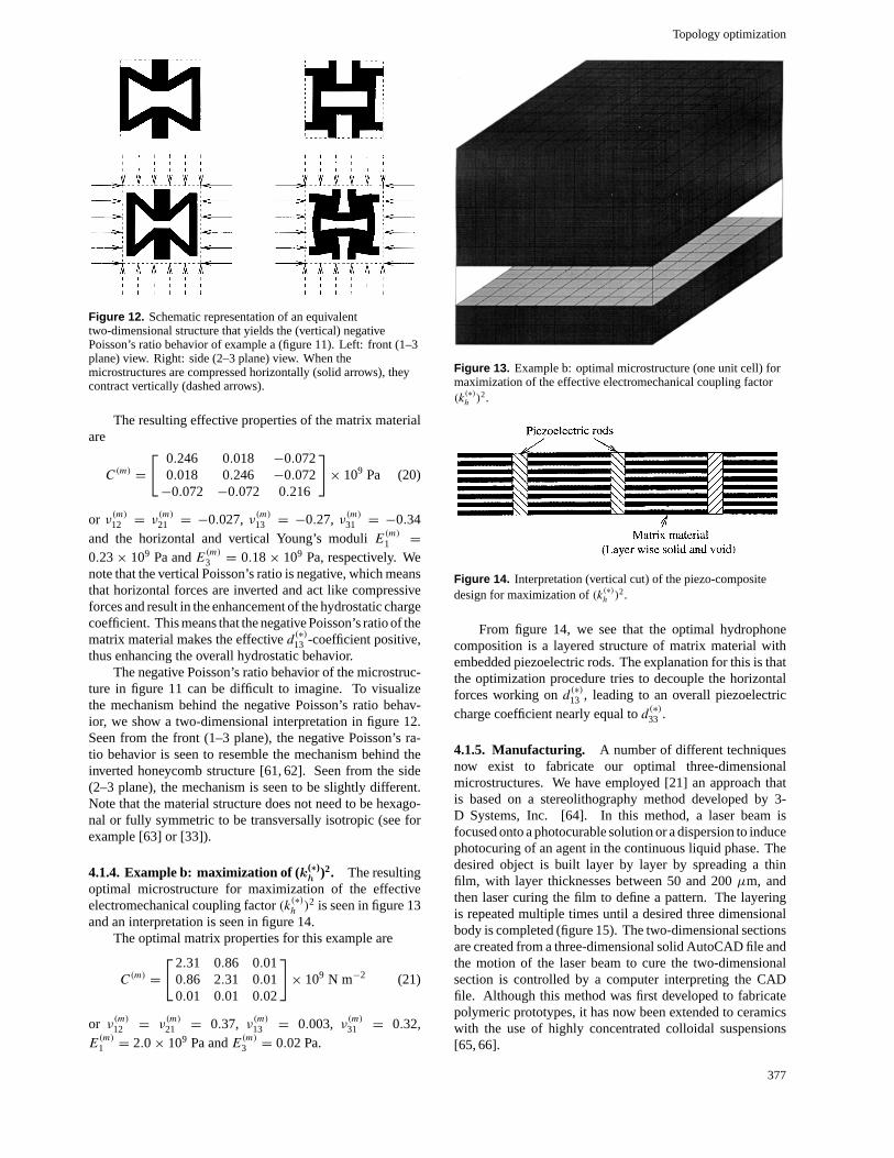
Topology optimization
Figure 12. Schematic representation of an equivalenttwo-dimensional structure that yields the (vertical) negativePoisson’s ratio behavior of example a (figure 11). Left: front (1–3plane) view. Right: side (2–3 plane) view. When themicrostructures are compressed horizontally (solid arrows), theycontract vertically (dashed arrows).
The resulting effective properties of the matrix materialare
C(m) =[ 0.246 0.018 −0.072
0.018 0.246 −0.072−0.072 −0.072 0.216
]× 109 Pa (20)
or ν(m)12 = ν(m)21 = −0.027, ν(m)13 = −0.27, ν(m)31 = −0.34
and the horizontal and vertical Young’s moduliE(m)1 =0.23× 10⁹ Pa andE(m)3 = 0.18× 10⁹ Pa, respectively. Wenote that the vertical Poisson’s ratio is negative, which meansthat horizontal forces are inverted and act like compressiveforces and result in the enhancement of the hydrostatic chargecoefficient. This means that the negative Poisson’s ratio of thematrix material makes the effectived(∗)13 -coefficient positive,thus enhancing the overall hydrostatic behavior.
The negative Poisson’s ratio behavior of the microstruc-ture in figure 11 can be difficult to imagine. To visualizethe mechanism behind the negative Poisson’s ratio behav-ior, we show a two-dimensional interpretation in figure 12.Seen from the front (1–3 plane), the negative Poisson’s ra-tio behavior is seen to resemble the mechanism behind theinverted honeycomb structure [61, 62]. Seen from the side(2–3 plane), the mechanism is seen to be slightly different.Note that the material structure does not need to be hexago-nal or fully symmetric to be transversally isotropic (see forexample [63] or [33]).
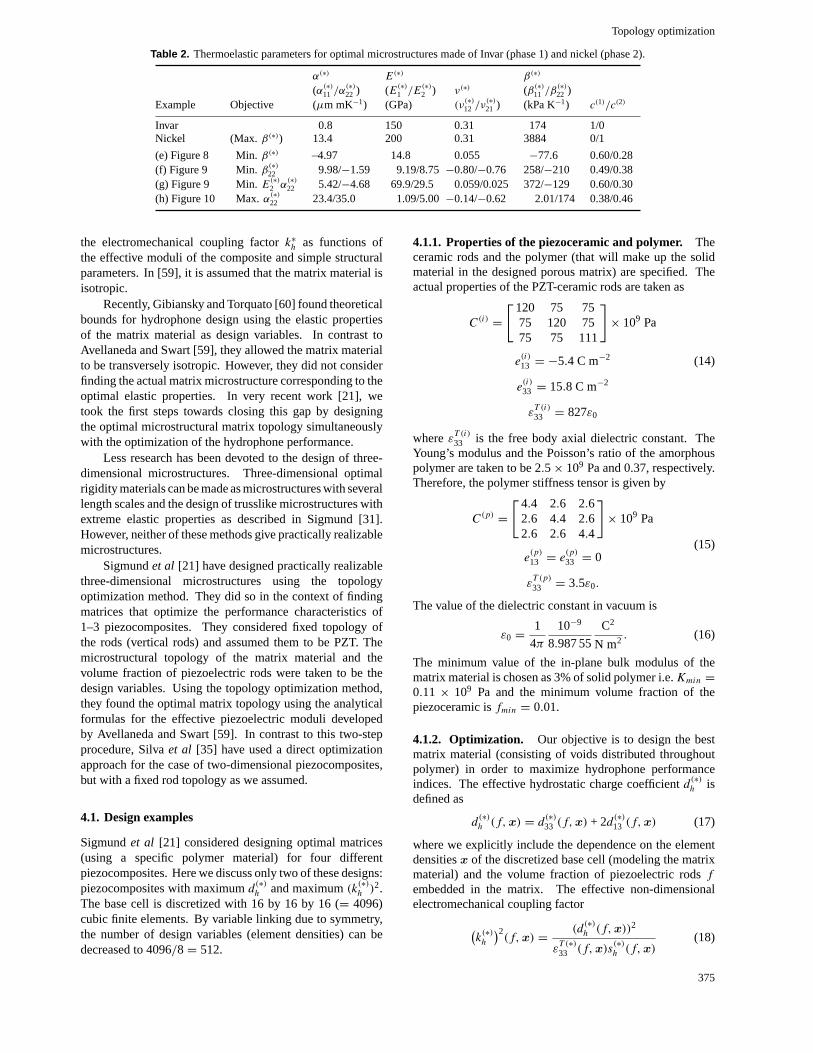
4.1.4. Example b: maximization of (k(∗)h )2. The resulting
optimal microstructure for maximization of the effectiveelectromechanical coupling factor(k(∗)h )
2 is seen in figure 13and an interpretation is seen in figure 14.
The optimal matrix properties for this example are
C(m) =[ 2.31 0.86 0.01
0.86 2.31 0.010.01 0.01 0.02
]× 109 N m−2 (21)
or ν(m)12 = ν(m)21 = 0.37, ν(m)13 = 0.003, ν(m)31 = 0.32,
E(m)1 = 2.0× 10⁹ Pa andE(m)3 = 0.02 Pa.
Figure 13. Example b: optimal microstructure (one unit cell) formaximization of the effective electromechanical coupling factor(k(∗)h )
2.
Figure 14. Interpretation (vertical cut) of the piezo-compositedesign for maximization of(k(∗)h )
2.
From figure 14, we see that the optimal hydrophonecomposition is a layered structure of matrix material withembedded piezoelectric rods. The explanation for this is thatthe optimization procedure tries to decouple the horizontalforces working ond(∗)13 , leading to an overall piezoelectriccharge coefficient nearly equal tod(∗)33 .
4.1.5. Manufacturing. A number of different techniquesnow exist to fabricate our optimal three-dimensionalmicrostructures. We have employed [21] an approach thatis based on a stereolithography method developed by 3-D Systems, Inc. [64]. In this method, a laser beam isfocused onto a photocurable solution or a dispersion to inducephotocuring of an agent in the continuous liquid phase. Thedesired object is built layer by layer by spreading a thinfilm, with layer thicknesses between 50 and 200µm, andthen laser curing the film to define a pattern. The layeringis repeated multiple times until a desired three dimensionalbody is completed (figure 15). The two-dimensional sectionsare created from a three-dimensional solid AutoCAD file andthe motion of the laser beam to cure the two-dimensionalsection is controlled by a computer interpreting the CADfile. Although this method was first developed to fabricatepolymeric prototypes, it has now been extended to ceramicswith the use of highly concentrated colloidal suspensions[65, 66].
377
O Sigmund and S Torquato
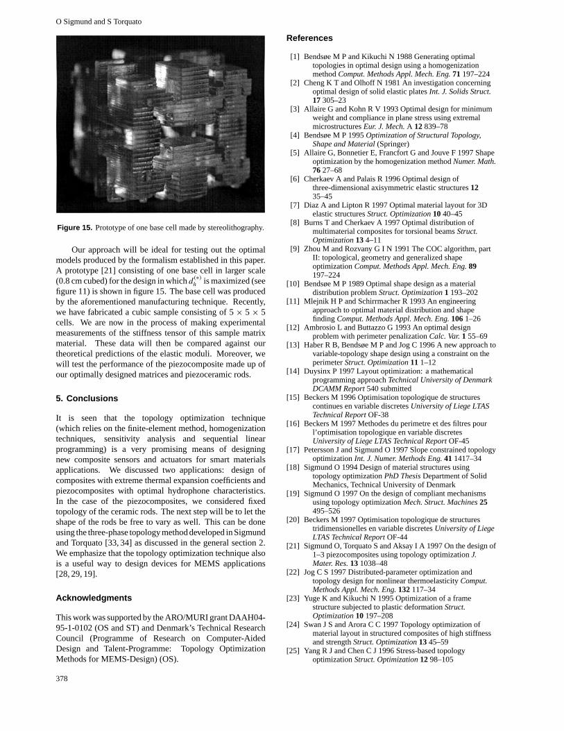
Figure 15. Prototype of one base cell made by stereolithography.
Our approach will be ideal for testing out the optimalmodels produced by the formalism established in this paper.A prototype [21] consisting of one base cell in larger scale(0.8 cm cubed) for the design in whichd(∗)h is maximized (seefigure 11) is shown in figure 15. The base cell was producedby the aforementioned manufacturing technique. Recently,we have fabricated a cubic sample consisting of 5× 5× 5cells. We are now in the process of making experimentalmeasurements of the stiffness tensor of this sample matrixmaterial. These data will then be compared against ourtheoretical predictions of the elastic moduli. Moreover, wewill test the performance of the piezocomposite made up ofour optimally designed matrices and piezoceramic rods.
5. Conclusions
It is seen that the topology optimization technique(which relies on the finite-element method, homogenizationtechniques, sensitivity analysis and sequential linearprogramming) is a very promising means of designingnew composite sensors and actuators for smart materialsapplications. We discussed two applications: design ofcomposites with extreme thermal expansion coefficients andpiezocomposites with optimal hydrophone characteristics.In the case of the piezocomposites, we considered fixedtopology of the ceramic rods. The next step will be to let theshape of the rods be free to vary as well. This can be doneusing the three-phase topology method developed in Sigmundand Torquato [33, 34] as discussed in the general section 2.We emphasize that the topology optimization technique alsois a useful way to design devices for MEMS applications[28, 29, 19].
Acknowledgments
This work was supported by the ARO/MURI grant DAAH04-95-1-0102 (OS and ST) and Denmark’s Technical ResearchCouncil (Programme of Research on Computer-AidedDesign and Talent-Programme: Topology OptimizationMethods for MEMS-Design) (OS).
References
[1] Bendsøe M P and Kikuchi N 1988 Generating optimaltopologies in optimal design using a homogenizationmethodComput. Methods Appl. Mech. Eng.71197–224
[2] Cheng K T and Olhoff N 1981 An investigation concerningoptimal design of solid elastic platesInt. J. Solids Struct.17305–23
[3] Allaire G and Kohn R V 1993 Optimal design for minimumweight and compliance in plane stress using extremalmicrostructuresEur. J. Mech.A 12839–78
[4] Bendsøe M P 1995Optimization of Structural Topology,Shape and Material(Springer)
[5] Allaire G, Bonnetier E, Francfort G and Jouve F 1997 Shapeoptimization by the homogenization methodNumer. Math.7627–68
[6] Cherkaev A and Palais R 1996 Optimal design ofthree-dimensional axisymmetric elastic structures1235–45
[7] Diaz A and Lipton R 1997 Optimal material layout for 3Delastic structuresStruct. Optimization1040–45
[8] Burns T and Cherkaev A 1997 Optimal distribution ofmultimaterial composites for torsional beamsStruct.Optimization134–11
[9] Zhou M and Rozvany G I N 1991 The COC algorithm, partII: topological, geometry and generalized shapeoptimizationComput. Methods Appl. Mech. Eng.89197–224
[10] Bendsøe M P 1989 Optimal shape design as a materialdistribution problemStruct. Optimization1 193–202
[11] Mlejnik H P and Schirrmacher R 1993 An engineeringapproach to optimal material distribution and shapefindingComput. Methods Appl. Mech. Eng.1061–26
[12] Ambrosio L and Buttazzo G 1993 An optimal designproblem with perimeter penalizationCalc. Var.1 55–69
[13] Haber R B, Bendsøe M P and Jog C 1996 A new approach tovariable-topology shape design using a constraint on theperimeterStruct. Optimization111–12
[14] Duysinx P 1997 Layout optimization: a mathematicalprogramming approachTechnical University of DenmarkDCAMM Report540 submitted
[15] Beckers M 1996 Optimisation topologique de structurescontinues en variable discretesUniversity of Liege LTASTechnical ReportOF-38
[16] Beckers M 1997 Methodes du perimetre et des filtres pourl’optimisation topologique en variable discretesUniversity of Liege LTAS Technical ReportOF-45
[17] Petersson J and Sigmund O 1997 Slope constrained topologyoptimizationInt. J. Numer. Methods Eng.411417–34
[18] Sigmund O 1994 Design of material structures usingtopology optimizationPhD ThesisDepartment of SolidMechanics, Technical University of Denmark
[19] Sigmund O 1997 On the design of compliant mechanismsusing topology optimizationMech. Struct. Machines25495–526
[20] Beckers M 1997 Optimisation topologique de structurestridimensionelles en variable discretesUniversity of LiegeLTAS Technical ReportOF-44
[21] Sigmund O, Torquato S and Aksay I A 1997 On the design of1–3 piezocomposites using topology optimizationJ.Mater. Res.131038–48
[22] Jog C S 1997 Distributed-parameter optimization andtopology design for nonlinear thermoelasticityComput.Methods Appl. Mech. Eng.132117–34
[23] Yuge K and Kikuchi N 1995 Optimization of a framestructure subjected to plastic deformationStruct.Optimization10197–208
[24] Swan J S and Arora C C 1997 Topology optimization ofmaterial layout in structured composites of high stiffnessand strengthStruct. Optimization1345–59
[25] Yang R J and Chen C J 1996 Stress-based topologyoptimizationStruct. Optimization1298–105
378

Topology optimization
[26] Duysinx P and Bendsøe M P 1998 Topology optimization ofcontinuum structures with local stress constraintsInt. J.Numer. Meth. Eng.431453–78
[27] Ou J S and Kikuchi N 1996 Integrated optimal structural andvibration control designStruct. Optimization12209–16
[28] Ananthasuresh G K, Kota S and Gianchandani Y 1994 Amethodical approach to the design of compliantmicromechanicsSolid-State Sensor and ActuatorWorkshoppp 189–92
[29] Larsen U D, Sigmund O and Bouwstra S 1997 Design andfabrication of compliant mechanisms and materialstructures with negative Poisson’s ratioJ.Microelectromech. Syst.6 99–106
[30] Sigmund O 1994 Materials with prescribed constitutiveparameters: an inverse homogenization problemInt. J.Solids Struct.312313–29
[31] Sigmund O 1995 Tailoring materials with prescribed elasticpropertiesMech. Mater.20351–68
[32] Sigmund O 1997 A new class of extremal compositessubmitted
[33] Sigmund O and Torquato S 1997 Design of materials withextreme thermal expansion using a three-phase topologyoptimization methodJ. Mech. Phys. Solids451037–67
[34] Sigmund O and Torquato S 1996 Composites with extremalthermal expansion coefficientsAppl. Phys. Lett.693203–5
[35] Silva E C N, Fonseca J S O andKikuchi N 1997 Optimaldesign of piezoelectric microstructuresComput. Mech.19397–410
[36] Bourgat J F 1997 Numerical experiments of thehomogenization method for operators with periodiccoefficientsLecture Notes in Mathematics(Berlin:Springer) pp 330–56
[37] Guedes J M and Kikuchi N 1991 Preprocessing andpostprocessing for materials based on the homogenizationmethod with adaptive finite element methodsComput.Methods Appl. Mech. Eng.83143–98
[38] Schultz P C and Smyth K T 1970 Ultra-low-expansionglasses and their structure in SiO2–TiO2 systemAmorphous Materials(New York: Wiley) ch 44,pp 453–62
[39] Kagaya H-M and Soma T 1993 Compression effect onspecific heat and thermal expansion of Si and GeSolidState Commun.85617–21
[40] Mary T A, Evans J S O, Vogt T andSleight W 1996 Negativethermal expansion from 0.3 to 1050 kelvin in ZrW2O8
Science27290–2[41] Hausch G, Bacher R and Hartmann J 1989 Influence of
thermomechanical treatment on the expansion behavior ofInvar and SuperinvarPhysicaB 16122–4
[42] Baughman R H and Galvao D S 1993 Crystalline networkswith unusual predicted mechanical and thermal propertiesNature365735–7
[43] Newnham R E and Ruchau G R 1991 Smart electro ceramicsJ. Am. Ceram. Soc.74463–80
[44] Smith W A 1991 Optimizing electromechanical coupling inpiezo composites using polymers with negative Poisson’sratioProc. IEEE Ultrasonics Symp.(Piscataway, NJ:IEEE)
[45] Christensen R M 1979Mechanics of Composite Materials(New York: Wiley)
[46] Pedersen P 1970 On the minimum mass layout of trussesSymp. on Structural Optimization (AGARD Conf. Proc.
36)pp 189–92[47] Schittkowski K 1994 Numerical comparison of non-linear
programming algorithms for structural optimizationStruct. Optimization7 1–19
[48] Hanson R J and Hiebert K L 1981 A sparse linearprogramming subprogramSandia National LaboratoriesTechnical ReportSAND81-0297
[49] Sigmund O and Petersson J 1998 Numerical instabilities intopology optimization dealing with checkerboards, meshdependencies and local minimaStruct. Optimization1668–75
[50] Schapery R A 1968 Thermal expansion coefficients ofcomposite materials based on energy principlesJ.Composite Mater.2 380–404
[51] Rosen B W and Hashin Z 1970 Effective thermal expansionand specific heat of composite materialsInt. J. Eng. Sci.8157–73
[52] Gibiansky L V and Torquato S 1997 Thermal expansion ofisotropic multi-phase composites and polycrystalsJ.Mech. Phys. Solidsat press
[53] Lakes R 1987 Foam structures with negative Poisson’s ratioScience2351038
[54] ASM 1993Properties and Selection (ASM Handbook 2)(Materials Information Society)
[55] Klicker K A, Biggers J V and Newnham R E 1991Composites of PZT and epoxy for hydrostatic transducerapplicationsJ. Am. Ceram. Soc.645
[56] Ting R Y, Shaulov A A and Smith W A 1992 Evaluation ofthe properties of 1–3 piezocomposites of a new leadtitanate in epoxy resinFerroelectrics13269–77
[57] Newnham R E 1986 Composite electroceramicsFerroelectrics681–32
[58] Chan H L W andUnsworth J 1989 Simple model forpiezoelectric ceramic/polymer in ultrasonic applicationsIEEE Trans. Ultrason. Ferroelectr. Freq. Control36434–41
[59] Avellaneda M and Swart P J 1995 Calculating theperformance of 1–3 piezocomposites for hydrophoneapplications: an effective medium approachCourantInstitute of Mathematics Working Paper
[60] Gibiansky L V and Torquato S 1997 Optimal design of 1–3composite piezoelectricsStruct. Optimization1323–8
[61] Almgren R F 1985 An isotropic three-dimensional structurewith Poisson’s ratio= −1 J. Elasticity12839–78
[62] Kolpakov A G 1985 Determination of the averagecharacteristics of elastic frameworksPMM J. Appl. Math.Mech. USSR49739–45
[63] Sigmund O 1996 Design and manufacturing of materialmicrostructures and micromechanismsProc. 3rd Int.Conf. on Intelligent Material, ICIM96 (Lyon, 1996), SPIEvol 2779, ed P Gobin (Bellingham, WA: SPIE) pp 856–66
[64] Jacobs P 1992Rapid Prototyping andManufacturing—Fundamentals of Stereolithography(Dearborn, MI: SME)
[65] Griffith M L and Halloran J W 1996 Freeform fabrication ofceramics via stereolithographyJ. Am. Ceram. Soc.792601–8
[66] Garg R, Prud’homme R K, Aksay I A, Liu F and Alfano R R1997 Optical transmission in highly-concentrateddispersions submitted
[67] Garg R 1997 Manufacturing of 3-d microstructures usingstereolithography in preparation
379