design sensitivity analysis and optimization tool...

Pergamon

Computing Systems in Engineering, Vol. 6, No. 2, pp. 151 175, 1995 Copyright © 1995 Elsevier Science Ltd

0956-0521(95)00006-2 Printed in Great Britain. All rights reserved 0965-0521/95 $9.50 + 0.00

DESIGN SENSITIVITY ANALYSIS AND OPTIMIZATION TOOL (DSO) FOR SHAPE DESIGN APPLICATIONS

KUANG-HuA CHANG, KYUNG K. CHOI, CHUNG-SHIN TSAI, CHIN-JUNG CHEN, BRIAN S. CHOI a n d XIAOMING YU

Center for Computer-Aided Design and Department of Mechanical Engineering, College of Engineering, The University of Iowa, Iowa City, IA 52242, U.S.A.

Abstract--The Design Sensitivity Analysis and Optimization (DSO) tool, developed initially for sizing design application, has been extended to support shape design applications of structural components. The new capabilities including shape design parameterization, error analysis and mesh adaptation, design velocity field computation, shape design sensitivity analysis, and interactive design steps, are discussed. These capabilities are integrated on the top of the DSO framework that includes databases, user interface, foundation class and remote module. The DSO allows the design engineer to easily create geometric, design, and analysis models; define performance measures; perform design sensitivity analysis (DSA); and carry out a four-step interactive design process that includes visual display of design sensitivity, what-if study, trade-off analysis, and interactive design optimization. Additionally, a 3-D tracked vehicle clevis is presented in this paper to demonstrate the new capabilities.

I. INTRODUCTION

Domain shape design problems in which the structural geometry is to be determined have attracted the attention of both academic and industrial researchers during the past two decades. The reason for this interest is that traditional sizing design variables have proven less effective than shape design variables for many applications.l'2 A typical example is that of a stress concentration at the boundary of a hole in a panel. Shape design is more effective for reducing stress concentration than sizing design since the former changes the geometrical shape of the hole instead of increasing or decreasing the thickness of the panel.

However, shape design optimization requires expertise in a number of areas, including CAD modelling, design parameterization, finite element analysis (FEA), finite element error analysis and mesh adaptation, design sensitivity analysis (DSA), and optimization (OPT). Accumu-lating adequate knowledge and appropriate tools together to perform shape design optimization is no small undertaking and requires a high degree of expertise. The objective of the Design Sensitivity Analysis and Optimization (DSO) tool 3 development is to provide design engineers with a convenient graphics-based design environment that integrates modeling and analysis tools to perform design optimization in an efficient and systematic way. The initial development that supports sizing design applications has generated a software foundation that allows extension for shape design applications. New capabilities include shape design parameterization, finite element error analysis and mesh adaptation, shape design velocity field computation, shape design sensitivity analysis, and

extension of the four-step design process 4 for shape design applications.

The rest of the paper is organized as follows. In Sec. 2, a brief description of the DSO is given. The three design stages that form the skeleton of the DSO are described in Secs 3 to 5. In these sections, only new capabilities for shape design applications are described. For a complete description of the DSO, the reader is referred to Ref. 3. A 3-D tracked vehicle clevis is presented in Sec. 6 to demonstrate DSO capabilities. The conclusions are given in Sec. 7.

2. DESIGN SENSITIVITY ANALYSIS AND OPTIMIZATION (DSO) TOOL

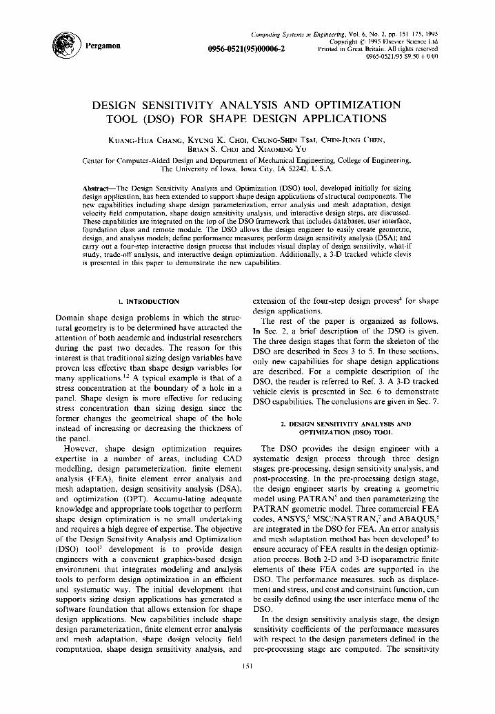
The DSO provides the design engineer with a systematic design process through three design stages: pre-processing, design sensitivity analysis, and post-processing. In the pre-processing design stage, the design engineer starts by creating a geometric model using PATRAN 5 and then parameterizing the PATRAN geometric model. Three commercial FEA codes, ANSYS, 6 MSC/NASTRAN, 7 and ABAQUS, 8 are integrated in the DSO for FEA. An error analysis and mesh adaptation method has been developed 9 to ensure accuracy of FEA results in the design optimization process. Both 2-D and 3-D isoparametric finite elements of these FEA codes are supported in the DSO. The performance measures, such as displacement and stress, and cost and constraint function, can be easily defined using the user interface menu of the DSO.

In the design sensitivity analysis stage, the design sensitivity coefficients of the performance measures with respect to the design parameters defined in the pre-processing stage are computed. The sensitivity

151

152 KUANG*HUA CHANG et al.

i f Generate Geometric ~ . ~ Define Design

and Rnite Element Parameters Models

PATRAN DSO

Perform Finite Element Error Analysis and Mesh

Adapta, on (Shape Applications Only)

DSO ANSYS/NASTRAN/ABAQUS

PATRAN DSO

Fig. 1. Pre-processing design stage.

Perform Finite Element~ Analysis I

ANSYS/NASTRAN//--" ]

,oos J1

Define Structural Performance Measures,

Cost and Constraint Func~ons

computation in the DSO uses the continuum DSA method, ]° which is more efficient, accurate, and general than the finite difference method.H Moreover, the sensitivity coefficients are computed outside the FEA codes using only post-processing data from the FEA codes. The sensitivity computation in the DSO has been integrated and automated so that the computation is launched and necessary data are transferred and accessed without the design engineer's interaction. As a result, in the DSO, the design engineer simply clicks on a menu button to compute design sensitivity coefficients.

In the post-processing design stage, to improve the structural performance or to achieve an optimum design, a four-step design process----design sensitivity display, what-if study, trade-off determination, and interactive optimization--can be used. The HARWELL subroutine library ~: and Design Optimization Tool (DOT) ]3 are used in the DSO to solve trade-off quadratic programming sub- problems and support interactive design optimization, respectively.

The three design stages form the foundation of the DSO. The design process and modeling and analysis tools have been integrated using a graphical menu- driven user interface developed using OSF MotiP 4 in the X Window '5 environment. Using the menu-driven user interface, design processes can be carried out using menu button instead of manually preparing and transferring data files, or analyzing results in an ad hoc way. The DSO is developed using a software framework, including the user interface, remote module, foundation class, and database. 3

3. PRE-PROCESSING DESIGN STAGE

The main objective of the pre-processing design stage is to formulate a design problem by defining a design model, including geometry and finite element modeling; design parameterizati0n; finite element analysis; finite element error analysis and mesh adaptation; and performance measure, cost, and constraint definition. Figure 1 illustrates the process.

3.1. Shape design parameterization The shape design parameterization method

developed in this study deals with geometric features. A geometric feature is a subset of the geometric boundaries of a structural component. For example, a fillet or a circular hole is a geometric feature that has certain characteristics associated with it and is likely to be chosen as the design boundary. A geometric feature with design parameters defined is a parameterized geometric feature. A parameterized geometric feature is treated as a single entity in the shape design process.

Geometric representation of entities in PATRAN. The design parameterization method developed in this study uses the basic PATRAN capability. In PATRAN all geometric entities are represented using parametric cubic (PC) lines, patches (surfaces), and hyperpatches (solids). A planar parametric cubic line is represented as 5

p(r) = a3 r3 + a2r 2 + a i r + ao

= [r 3 r 2 r II a2

4×2

=RA, re[0,1] (1)

where p ( r ) = [Px,Py], r is the parametric direction of the line with domain [0, 1], and a~ = [a~x, aiy], i = 0 to 3, are the algebraic coefficients of the curve.

From Eq. (1), it is obvious that any component of the parametric cubic line can change the sign of its slope at most twice, and can have only one inflection point. Consequently, parametric cubic (PC) entities such as PC lines and PC patches minimize the possibility of oscillatory boundaries in the design process. 2 However, certain geometric features with pre-defined shapes or sophisticated geometry, such as a circular hole, cannot be represented by a single cubic geometric entity. To minimize modeling errors, it is necessary to model such a boundary by breaking

Design Sensitivity Analysis and Optimization Tool

( a ) ( b )

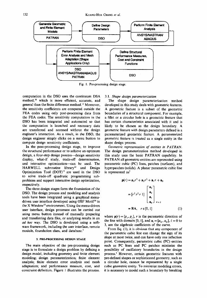
Fig. 2. Pre-defined geometric features.

I dp3

153

it into small pieces. In the design process, these pieces must be "glued" together as one geometric feature by linking design parameters appropriately. For shape design, planar parametric cubic lines and the spatial parametric bicubic patches are utilized to represent design boundaries of 2-D and 3-D structural components, respectively.

Three-step shape design parameterization method. A three-step shape design parameterization method has been developed, t6 The first step is to create a geometric feature by grouping a number of inter- connected geometric entities and defining the type of the geometric feature. The second step is to define design parameters for each geometric feature. Geometric features that are frequently used in the construction of structural components can be put in a library of predefined geometric features. The design engineer can parameterize these features by simply selecting the associated predefined shape design parameters from the user interface menu. For example, a circular hole and the tapered slot shown in Fig. 2 can be defined as predefined geometric features and put in the library. On the other hand, geometric features that are not included in the library must be defined as user-defined features. To generate a para-

meterized user-defined geometric feature, the desgin engineer can use the design parameter definition within the geometric entities and link design parameters across the entities. The third step is to link design parameters across parameterized geometric features, if necessary.

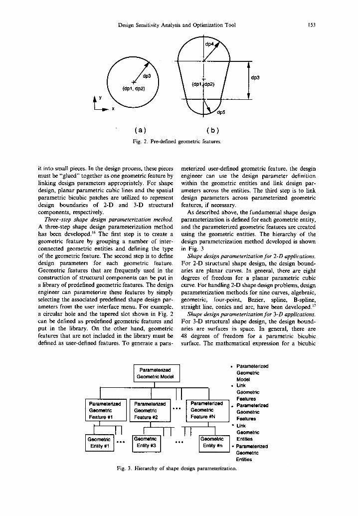
As described above, the fundamental shape design parameterization is defined for each geometric entity, and the parameterized geometric features are created using the geometric entities. The hierarchy of the design parameterization method developed is shown in Fig. 3

Shape design parameterization for 2-D applications. For 2-D structural shape design, the design boundaries are planar curves. In general, there are eight degrees of freedom for a planar parametric cubic curve. For handling 2-D shape design problems, design parameterization methods for nine curves, algebraic, geometric, four-point, Bezier, spline, B-spline, straight line, conics and arc, have been developed/7

Shape design parameterization for 3-D applications. For 3-D structural shape design, the design boundaries are surfaces in space. In general, there are 48 degrees of freedom for a parametric bicubic surface. The mathematical expression for a bicubic

I I Parameterized

Geometric Feature #1

[I I I Geometric

Entty#1 I °°°

I Parameterized I Geometric Model

I

I II Parameterized • Geometric "" Feature #2

I i II

Geometric I • ° . . Entity #3 I

I Parameterized I ° Geometric Feature #N

I ° II I

[G~metric I Entity#n I • I

• Parameterized Geometric Model

• Link Geometric Features Parameterized Geometric Features Unk Geometric Entities Parameterized Geometric Entities

Fig. 3. Hierarchy of shape design parameterization.

154

parametric surface is

KUANG-HUA CHANG et al.

3 p ( r , s ) = ~ aljrls j

U= 0

= [r 3 r 2 r 1]

a33 a32 a31

a23 a22 a21 a~3 a~2 aH

a03 a02 a01

= R A S T, (r ,s)6[0,1] × [0,1]

a3o 820 /

a,0/ a00 A 4x4×3 L 1 J 4 x l

(2)

where p(r, s) = [Px,Py,Pz], ao = [aox, aoy, aoz] is the algebraic coefficient of the surface, and r and s are the parametric directions of the geometric entity.

To support 3-D shape design applications, design parameterization methods for algebraic, geometric, 16-point, Bezier, plane surface, cylindrical surface, ruled surface, and surface of revolution have been developedJ 7 A geometric surface is taken a s an example to explain how a 3-D solid can be parameterized.

Similar to a geometric curve, a geometric surface is represented by the positions, tangent vectors, and twist vectors at the four corner points of the surface, as shown in Fig. 4. To parameterize the geometric surface, all 48 geometric coefficients in the B matrix can be defined as shape design parameters, i.e.

B =

Poo Pol Poo ~ Pol w

Plo Pn Plo ~ P f f

Poo ~ pol ~ Poo ~ Pol uw

pjo ~ pn u plo ~ pll ~w 4 × 4 x 3

(3)

To aid the design engineer to easily parameterize the geometric curve, a design parameterization menu shown in Fig. 5 is implemented.

Automatic design parameter linking. The automatic linking capability provided in the DSO ensures C°-continuity of the design boundary in the design process. The DSO automatically searches all boundary grid points, identifies boundary lines or surfaces, and determines proper ways of linking the

conjunction grid point to ensure C°-continuity. To ensure a Cl-continuous design boundary, the design engineer needs to use the manual linking capabilities that are similar to those of sizing design applications)

3.2. Finite element analysis

Isoparametric finite elements, a 2-D 8-node and a 3-D 20-node, are supported in the DSO for 2-D and 3-D shape design applications, respectively. Since the basic theories for these elements in the three FEA codes, ANSYS, MSC-NASTRAN, and ABAQUS, are the same, one sensitivity analysis code can support these elements in the three FEA codes. The DSO finite element types for shape design applications and their corresponding types in the analysis codes are listed in Table 1.

3.3. Finite element error analys& and mesh adaptation

One of the most difficult tasks in shape design optimization is to maintain the accuracy of FEA results during the design process. In analysis of a 3-D structural component with a complicate geometric shape, a refined finite element mesh is necessary to accurately capture stress concentration. Thus, the dimension of finite element models tends to be very large for 3-D structural components. Furthermore, the finite element mesh is continuously changing since the geometry of the design model is changing during the design process? '2 Maintaining accuracy of finite

~ rve 2

.z,:,2.-r" A Z \ Y ,';w °°.Y Ourve 4 \ i'/N Y

¢,o

Fig. 4. Geometric surface.

Design Sensitivity Analysis and Optimization Tool 155

Fig. 5. Design parameterization menu.

element analysis is difficult since finite element meshes may become distorted due to shape change.

Finite element error analysis and mesh adaptation procedures are used in the DSO to ensure accuracy of the analysis model. The Simple Error Estimator developed by Zienkiewicz 18'~9 is used for finite element error analysis. An interactive mesh adaptation algorithm that uses error information as a criterion for element size adjustment has been developed. 9 PATRAN's meshing capabilities are utilized to provide interactive mesh refinement capability.

To perform mesh adaptation, a preliminary finite element model with coarse mesh is generated first using PATRAN. The mesh is then refined according to the specified mesh refinement criterion. The mesh refinement criterion 6 adopted in the DSO requires that the following inequalities be satisfied at all elements of the refined model,

qi~< 4, i = 1, number of elements (4)

where qi is the percentage error of the ith element in the energy norm.

Since the error estimate is computed for each element, it can be displayed over the structural domain using color contours to identify regions with large error. The ratio between element percentage

error qi and refinement criterion f/ determines elements that need further refinement, and the amount of refinement. High stress concentration areas are of critical concern for design engineers. To ensure adequate accuracy of FEA stress results, a refined mesh must be used at critical regions. To what extent the mesh should be refined is difficult to determine in advance. Large errors may occur in areas with low stress. Only regions of high stress concentration and large error accumulation need to be refined. In the DSO, both stress and error contour plots are displayed in a PATRAN window, to help the design engineer in refining the mesh.

4. DESIGN SENSITIVITY ANALYSIS STAGE

In shape DSA, shape of the structural domain is treated as the design parameter. The relationship between shape variations of a continuous domain and the resulting variations in structural performance measures can be described using the material derivative of continuum mechanics. ~° Using the material derivative, the concept of design velocity field is introduced to describe movements of material points resulting from a change in the shape of the structural boundary.l°

Table 1. Finite element types in the DSO for shape applications

Finite MSC/ elements DSO ANS Y S NASTRAN ABAQUS

2-D Solid EL2D STIF82 CQUAD8 S8R 3-D Solid EL3D STIF95 CHEXA C3D20R

156 KUANG-HUA CHANG et al.

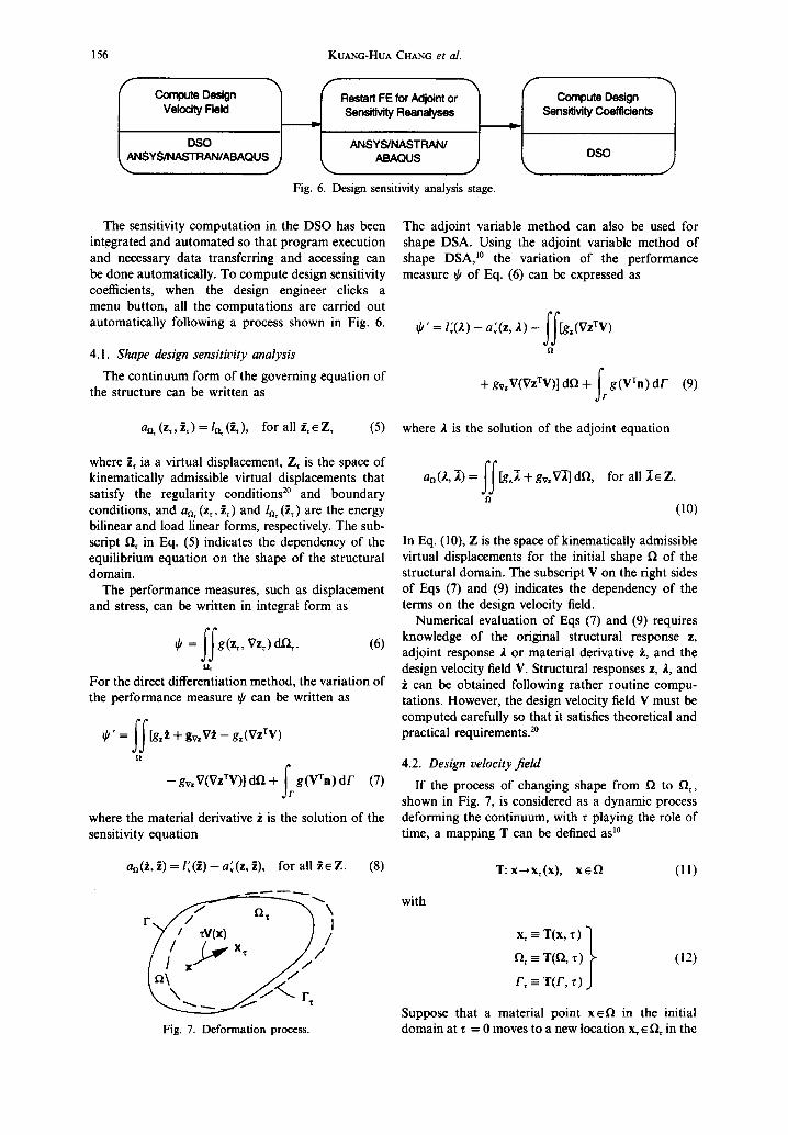
Compute Design ~'~ Velocity Reid /

| I Restart FE for Adjoint or '~ Sensitivity Reanalyses -I ) ANSYS/NASTRAN/

ABAQUS

Fig. 6. Design sensitivity analysis stage.

Compute Design 1 Sensitivity Coefficients

L~ DSO

The sensitivity computation in the DSO has been integrated and automated so that program execution and necessary data transferring and accessing can be done automatically. To compute design sensitivity coefficients, when the design engineer clicks a menu button, all the computations are carried out automatically following a process shown in Fig. 6.

4.1. Shape design sensitivity analysis The continuum form of the governing equation of

the structure can be written as

The adjoint variable method can also be used for shape DSA. Using the adjoint variable method of shape DSA, ~° the variation of the performance measure ~b of Eq. (6) can be expressed as

~0' = I ; 0 . ) - a ; ( z , ~.) - ~f[g,(VzrV) f l

+gwV(VzXV)]d~ + I g(VXn)dr (9) jr

an, (z,, i , ) = lo~ (i,), for all i , e Z, (5) where/t is the solution of the adjoint equation

where ~ ia a virtual displacement, Z, is the space of kinematically admissible virtual displacements that satisfy the regularity conditions 2° and boundary conditions, and an, (z,, ~.,) and ln, (~,) are the energy bilinear and load linear forms, respectively. The subscript D~ in Eq. (5) indicates the dependency of the equilibrium equation on the shape of the structural domain.

The performance measures, such as displacement and stress, can be written in integral form as

~b = I I g ( z , , Vz,) dfl,. (6)

f ir

For the direct differentiation method, the variation of the performance measure ~b can be written as

~k' = II[g=~ + gv=Vi - g,(VzTV)

f l

-- gv=V(VzTV)] dfl + t g(VTn) d r (7) Jr

where the material derivative ~, is the solution of the sensitivity equation

an(2, ~) = ff[gz~+gv, V~] dll, for all ~[~Z. fl

(10)

In Eq. (10), Z is the space of kinematically admissible virtual displacements for the initial shape f~ of the structural domain. The subscript V on the right sides of Eqs (7) and (9) indicates the dependency of the terms on the design velocity field.

Numerical evaluation of Eqs (7) and (9) requires knowledge of the original structural response z, adjoint response ). or material derivative ~, and the design velocity field V. Structural responses z, 2, and

can be obtained following rather routine computations. However, the design velocity field V must be computed carefully so that it satisfies theoretical and practical requirements, s°

4.2. Design velocity field If the process of changing shape from fl to f~,,

shown in Fig. 7, is considered as a dynamic process deforming the continuum, with z playing the role of time, a mapping T can be defined as l°

an(i,~.)=l'([)--a~(z,~), for all ~.eZ. (8)

\ r l

/ /

Fig. 7. Deformation process.

T: x---}x,(x), x~Q (II)

with

x' = T ( x ' Q t ~, = T(I'I, z) F, = T(F, z)

(12)

Suppose that a material point x ef~ in the initial domain at T = 0 moves to a new location x, e fl, in the

Design Sensitivity Analysis and Optimization Tool

perturbed domain. The design velocity field V can be defined as

dx~ dT(x,z) aT(x,-r) V(x~, z) - d'c dz ~gz (13)

In the neighborhood of initial time z = 0, assuming a regularity hypothesis and ignoring higher-order terms, T can be approximated by

T(x, r) = T(x, 0) + z aT(x, 0) & + O(~:)

,~ x + zV(x, 0) (14)

where x = T(x, 0) and V(x) = V(x, 0).

4.3. Numerical implementation for velocity fieM computation

In the DSO, both the boundary displacement 2L22 and isoparametric mapping methods 23 are implemented. In the boundary displacement method, the boundary velocity field is computed first using the isoparametric mapping method. The domain velocity field is then computed by solving an auxiliary structure that is represented by an elliptic differential equation. In the isoparametric mapping method, both the boundary and domain velocity fields can be computed simultaneously using matrix multiplication very efficiently.

Velocity fieM computation using the boundary displacement method. Computation of the boundary velocity field for the discretized finite element model is directly related to the design parameterization that is defined for the geometric model. As discussed previously, the most primitive design parameters are defined on the geometric entities. In order to parameterize the geometric features, design parameter linking must be carried out across geometric entities. Consequently, the boundary velocity field must be computed for all the geometric entities on which the associated shape design parameters, either independent or dependent, are defined.

The boundary velocity field is computed using the isoparametric mapping method, as shown in Eqs (15a) and (15b) for 2-D and 3-D structural components, respectively,

Vl x 2 = [ r3 r2 r 1]

6a3

6a2 L ,~a, | 6aoJ 4x2

= R 6 A , re[0,1] (15a)

Vl x 3 = [ r3 r2 r 1]

6a33 6a32 6a31 6a3o 1 6a23 c~a22 6a2, 6a2o| c~al3 c~al2 ~ali ~ajo / 6a03 6a02 6aol 6aoo_l 4x4x3

157

Boundary Velocity Field

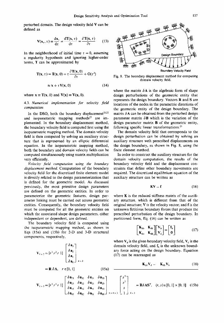
Fig. 8. The boundary displacement method for computing domain velocity field.

where the matrix 6A is the algebraic form of shape design perturbations of the geometric entity that represents the design boundary. Vectors R and S are locations of the nodes in the parametric directions of the geometric entity of the design boundary. The matrix 6 A can be obtained from the perturbed design parameter matrix 6B which is the variation of the design parameter matrix B of the geometric entity, following specific linear transformations. 23

The domain velocity field that corresponds to the design perturbation can be obtained by solving an auxiliary structure with prescribed displacements on the design boundary, as shown in Fig. 8, using the finite element method.

In order to construct the auxiliary structure for the domain velocity computation, the results of the boundary velocity field and the displacement constraints that define other boundary movements are required. The discretized equilibrium equation of the auxiliary structure can be written as

K V = f (16)

where K is the reduced stiffness matrix of the auxiliary structure, which is different from that of the original structure; V is the velocity vector; and f is the unknown fictitious boundary forces that produce the prescribed perturbation of the design boundary. In partitioned form, Eq. (16) can be written as

,qFvq= ,~ ,~JLVJ [~] (17)

where V b is the given boundary velocity field, V d is the domain velocity field, and fb is the unknown boundary force acting on the design boundary. Equation (17) can be rearranged as

Kdd Vd = -- Kdb Vb (18)

S 2 = R6 AS T,

4×1

(r, s)e[0, 11 x [0, 1] (15b)

158 KUANG-HUA CHANG e l a l .

which defines a linear relation between the boundary and domain velocity fields. The same finite element code used for analysis can be used to compute the displacement field of the auxiliary structure, i.e. the domain velocity field, which naturally satisfies the regularity and linearity requirements.

An important characteristic of the elasticity problem (elliptic partial differential equation), is that the solution trajectory tends to maintain orthogonality. As a result, the updated mesh that is obtained from the velocity field tends to maintain orthogonality.

Velocity field computation using the isoparametric mapping method. In PATRAN, the patches are represented by Eq. (2) and hyperpatches are represented by

3 4 p(r,s, t ) = ~ a~krisJtk= ~ avkr n is4 Jt 4 k

id, k = 0 i,),k - I

= r 3SAijl TT + r2SAij2 T T + rSAij 3 T T + SAij 4 T T,

(r,s,t)~[O, 1]×[O, 1]x[O, 1] (19)

where R = [r 3 r 2 r l ] , S = [s 3 S 2 S 1], T = [t 3 t 2 t 1], and matrices A0k=[a~k] are the algebraic coefficient matrices of the hyperpatch. The velocity fields, there- fore, can be obtained from variations of the above equations, i.e. Eq. (15b) for 2-D applications, and

V = 6p(r, s, t) = r3S~AijlTT + r2S3Aij2 TT

+ rS6Aij3 TT + S6Aij4 TT (20)

for 3-D applications, where 6A~k are the perturbed algebraic coefficient matrices of the hyperpatch.

Matrices 6A~,, ~ = 1, 4 can be obtained from the design perturbation matrices 6B~ by

6A~ = MaiM 6BiM T (21)

where A, = [ a j , M~ is a single specific element of the matrix M, and the geometric coefficient matrices 6Bl, 6B2, 3B3, and 6B4, are the design perturbation matrices of the geometric hyperpatch. 5 Design perturbation matrices fib i can be obtained from perturbation of the geometric coefficient matrices Bi following design parameterization. Geometric coefficients in a geometric hyperpatch are defined in Ref. 5.

Note that the isoparametric mapping method is extremely efficient compared to the boundary displacement method. However, velocity field obtained using the mapping method will not generate finite element mesh as regular as the one obtained from boundary displacement method 23 which may be problematic for some applications.

4.4. Numerical implementation for shape design sensitivity computation

Numerical evaluation of Eqs (7) and (9) requires knowledge of the original structural response z, adjoint response 2 or material derivative z, and the design velocity field V. The design velocity field V can be computed using the methods described above. The solution z of Eq. (6) is obtained by structural FEA in the pre-processing design stage. The solution 2 of the adjoint equation, Eq. (10), or solution i of the sensitivity equation, Eq. (8), can be obtained by restarting the FEA code that was used to solve Eq. (5) with additional loading vectors that are defined by the right side of Eqs (8) or (11). Notice that Eq. (10) has to be solved for each displacement or stress performance measure that has a corresponding adjoint load. On the other hand, for the direct differentiation method, Eq. (8) must be solved for NL × NDV times, where NL and NDV are numbers of loads and design parameters, respectively. No adjoint structural or sensitivity analysis is necessary for compliance, natural frequency, buckling load, volume, and mass performance measures.

Depending on which finite element code was utilized to analyze the original structure, an appropriate analysis input data file is generated to restart that FEA for the additional adjoint or fictitious load cases. To restart the analysis, the files from the original analysis that contain the decomposed stiffness matrix are utilized again.

After adjoint or sensitivity structural reanalysis, the finite element interface program of the DSO is executed to get adjoint or sensitivity responses, £ or z, from the databases of the analysis codes. Then, the DSO performs Gauss integration to compute sensitivity coefficients, using Eqs (7) or (9).

5. POST-PROCESSING DESIGN STAGE

One of the most difficult tasks in shape design applications is the development of an interactive design process that provides effective visualization of design sensitivity information and supports auto- mation of the shape design process. An integrated and automated design environment must be developed to minimize difficulty in handling tedious routine operations, such as control of execution of programs and data manipulation. This shape design environment must also provide tools for easy interpretation of design results.

The post-processing design stage in the DSO is a four-step interactive design process, which includes design sensitivity display, what-if study, trade-off determination, and design optimization. 3'4 This interactive design environment, shown in Fig. 9, allows the design engineer to improve designs, using the design sensitivity coefficients. The first three design steps help the design engineer understand the sturctural behavior of the current design and suggest how the design engineer can achieve better designs.


Prepare Data Files to Display

Sensitivity Information

DSO l - - - - - . - - IP

Try out Alternative Designs/What-if

Study

DSO ANSYS/NASTRAN/

ABAQUS

# Determine

Design Trade-offs

DSO

Interactive Design Mode

Fig. 9. Post-processing design stage,

Ii erform Design " Optimization

DSO DOT

NSYS/NASTRAN/ ABAQUS ~"

Batch Design Mode

The last design step launches a commerical optimization code. The post-processing stage in the DSO provides sufficient design information and design suggestions for the design engineer to make appropriate design decisions.

The design engineer can use the four-step design process in various ways, depending on the engineer's goal. For instance, if the design engineer is looking for an improved design, the design engineer can go through the first three design steps to understand structural design trends of the current design and then change the design based on the design engineer's understanding of structural behavior or suggestions made by the DSO. Once changes are made through a what-if study, the DSO automatically updates the design model, analyzes it, computes its design sensitivity coefficients, and gets ready for the next design iteration. This is the so-called interactive design mode, and will be illustrated further using the clevis example.

Instead of using the interactive mode, the design engineer can also ask the design optimization module of the DSO to perform a certain number of design iterations in batch mode. After several design iterations, the design engineer can return to the first three design steps to display the design sensitivity coefficients and perform several what-if or trade-off studies, before deciding the next design direction. When an optimum design is obtained using the optimization algorithm, the design engineer might again go through design sensitivity display, what-if, or trade-off design steps to get a thorough understanding of the structural behavior of the optimum design or to provide tolerance information for the manufacturer. 3

5.1. Design sensitivity display

The design sensitivity matrix contains valuable information for the design engineer to understand structural behavior and make appropriate design changes. To evaluate design sensitivity coefficients by reading the numerical values is, however, difficult and impractical for general design applications. For this reason, the sensitivity display capability in the DSO not only displays the full design sensitivity coefficients in the spreadsheet 3 but also plots the sensitivity

coefficients of a performance measure in the steepest descent direction using a PATRAN contour plot and/or a bar chart.

5.2. What -if study

The what-if study provides the design engineer with a first-order prediction of the structural performance measures by Taylor series expansion about the current design,

O;+~b~ i (22) ~ ~b b + 6bj

where q/ is the ith performance measure, (a~bi/Obj) is the design sensitivity coefficient of the ith performance measure with respect to the j th design parameter, and 6bi is the design perturbation of the ith design parameter. The what-if study gives a quick first-order approximation of structural performance measures at the perturbed design, without going through a new FEA.

The DSO supports three types of perturbations: perturbation that the design engineer provides, perturbation in the steepest descent direction of a performance measure with a given step size, and perturbation in the direction found by a trade-off determination, with a specific step size. The design engineer can easily and conveniently interact with the DSO through the user interface menu to perform what-if studies.

The what-if study results and the current performance measures can be displayed in a spreadsheet, and in PATRAN color plots or bar charts. These displays allow the design engineer to instantly identify the predicted structural responses of the perturbed design. Once the design engineer finds a satisfactory design after trying out different design alternatives in an approximation sense, the design engineer can ask the DSO to update the design model following the computation process described in Fig. 10. Note that it requires only a menu button click to launch the computation shown in Fig, 10. The design engineer can use the what-if study and design model update capabilities to perform a number of design iterations interactively.


~ ~ ~ Perform Finite~'NI ~initeElement~ ~ (~UpdatePerformanc~e I ~.fame.,,e~ I I .Element Static and [ I Error Analysis I J ~ NO I Measures, cost andl I ~"--~,~.%. I

I ~ ~ l e l ~ ~ a e d p ; t . ~ n ~ Constraint Funetions~ C~:~c:~n~s J

41, R e p e a t e d A i I Fi i Pe r fo rm i

\ oso 1 , I . . . . . . . . . . . . . . . . . . . . . . . . . . . . . . . . . . . . . . . . . . . . . . . . . . . . . . . . . . . .

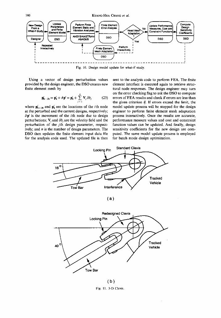
Fig. 10. Design model update for what-if study.

Using a vector of design perturbation values provided by the design engineer, the DSO creates new finite element mesh by

p~+ab= ~ + 6p'=lg,+ ~ Vjrbj (23) i = 1

where i~+~b and 1~ are the locations of the ith node at the perturbed and the current designs, respectively; 6p i is the movement of the ith node due to design perturbations; Vj and 6bj are the velocity field and the perturbation of the jth design parameter, respectively; and n is the number of design parameters. The DSO then updates the finite element input data file for the analysis code used. The updated file is then

sent to the analysis code to perform FEA. The finite element interface is executed again to retrieve structural node responses. The design engineer may turn on the error checking flag to ask the DSO to compute errors of FEA results and check if errors are less than the given criterion r 7. If errors exceed the limit, the model update process will be stopped for the design engineer to perform finite element mesh adaptation process interactively. Once the results are accurate, performance measure values and cost and constraint function values can be updated. And finally, design sensitivity coefficients for the new design are computed. The same model update process is employed for batch mode design optimization.

Standard Clevis

Vehicle

(a)

Redesigned Clevis , Locking~Pin ~ .

, ° j / Vehicle

(b) Fig. 11. 3-D Clevis.


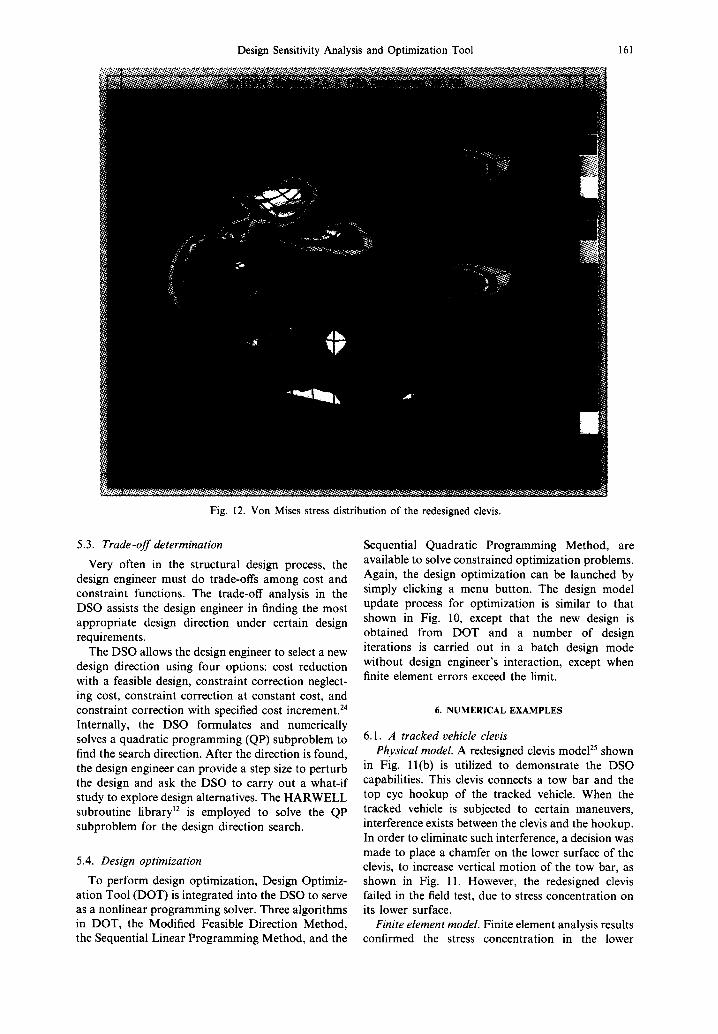
Fig. 12. Von Mises stress distribution of the redesigned clevis.

5.3. Trade-off determination

Very often in the structural design process, the design engineer must do trade-offs among cost and constraint functions. The trade-off analysis in the DSO assists the design engineer in finding the most appropriate design direction under certain design requirements.

The DSO allows the design engineer to select a new design direction using four options: cost reduction with a feasible design, constraint correction neglect- ing cost, constraint correction at constant cost, and constraint correction with specified cost increment. 24 Internally, the DSO formulates and numerically solves a quadratic programming (QP) subproblem to find the search direction. After the direction is found, the design engineer can provide a step size to perturb the design and ask the DSO to carry out a what-if study to explore design alternatives. The HARWELL subroutine library ~2 is employed to solve the QP subproblem for the design direction search.

5.4. Design optimization

To perform design optimization, Design Optimiz- ation Tool (DOT) is integrated into the DSO to serve as a nonlinear programming solver. Three algorithms in DOT, the Modified Feasible Direction Method, the Sequential Linear Programming Method, and the

Sequential Quadratic Programming Method, are available to solve constrained optimization problems. Again, the design optimization can be launched by simply clicking a menu button. The design model update process for optimization is similar to that shown in Fig. lO, except that the new design is obtained from DOT and a number of design iterations is carried out in a batch design mode without design engineer's interaction, except when finite element errors exceed the limit.

6. NUMERICAL EXAMPLES

6.1. A tracked vehicle clevis Physical model. A redesigned clevis model 25 shown

in Fig. l l(b) is utilized to demonstrate the DSO capabilities. This clevis connects a tow bar and the top eye hookup of the tracked vehicle. When the tracked vehicle is subjected to certain maneuvers, interference exists between the clevis and the hookup. In order to eliminate such interference, a decision was made to place a chamfer on the lower surface of the clevis, to increase vertical motion of the tow bar, as shown in Fig. 1 1. However, the redesigned clevis failed in the field test, due to stress concentration on its lower surface.

Finite element model. Finite element analysis results confirmed the stress concentration in the lower

Element 818 772 268

KUANG-HUA CHANG et al. 162

Fig. 13. Finite element model and boundary conditions.

surface, as shown in Fig. 12, under boundary conditions applied at the four half pins, as shown in Fig. 13. Note that the high stresses found in four half pins are artificial due to applications of boundary conditions. The material used is SAE 1045 with properties Young's modulus E = 10.5 x 106psi, Poisson's ratio v =0.3, and yielding stress 185 ksi. The finite element model has 928 20-node isoparametric elements (ANSYS STIF95) and 5369 nodes, with 16,000 degrees of freedom.

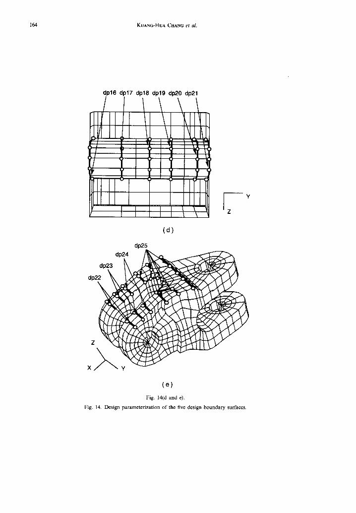
Design model definition. The objective of designing the redesigned clevis is to reduce the stress values below 75% of the material yield stress by altering the five boundary surfaces, without significantly increasing its weight. The five design boundary surfaces are front, rear, front slot, rear slot, and bottom, as shown in Fig. 14.

The geometric patch format was chosen to parameterize the five design boundary surfaces. For the front surface, Y-coordinates of the seventeen grid points are linked as five independent shape design parameters, as illustrated in Fig. 14(a). For the front surface, C°-continuity is retained by the design parameter linking at the grids of interpatch boundaries. Moreover, CJ-continuity is retained since the tangent vectors and twist vectors are invariant. For the rear surface, Y-coordinates are allowed to vary. For the two slots, X-coordinates are allowed to vary. For the bottom surface, Z-coordinates of the grid points are defined as shape design parameters. As a consequence, 25 independent design parameters are defined for the five surfaces to parameterize the clevis.

The volume and maximum von Mises stresses at integration points of each finite element, excluding

elements in the half pins with artificially high stresses, are defined as the performance measures. There are 668 stress and 1 volume performance measures defined. The maximum stresses are found at elements 772 and 818, as shown in Figs 12 and 13. The volume measure is chosen as cost function, with value 89.71 in 3 at initial design. These 668 stress measures are defined as constraints with an upper bound of 138.75 ksi (0.75 x Cry). The five finite elements with high stresses shown in Figs 12 and 13 are listed in Table 2, together with their stress values at the initial design.

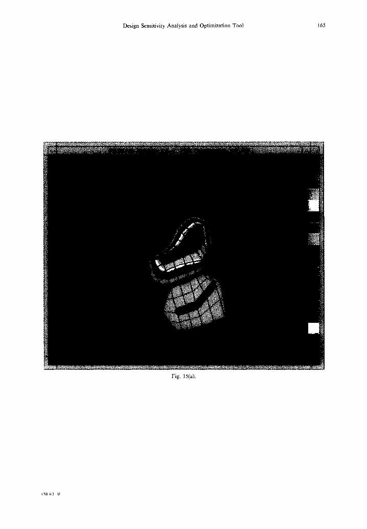
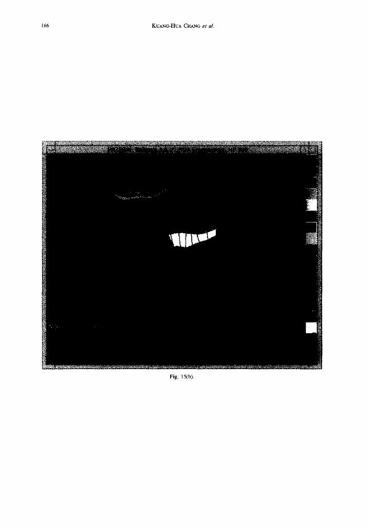
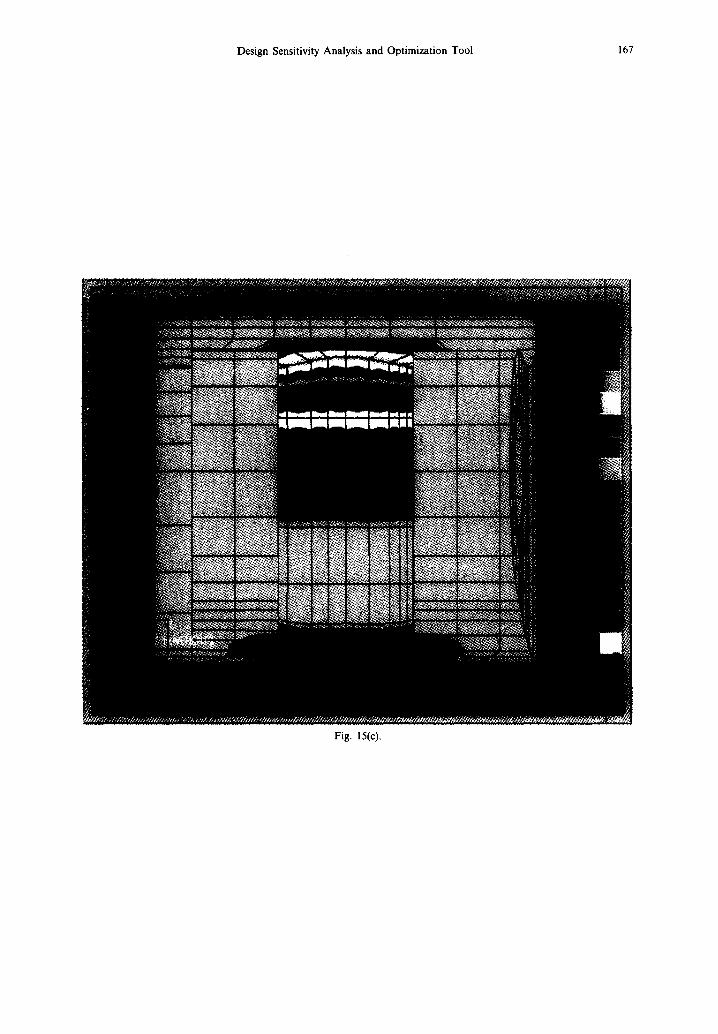
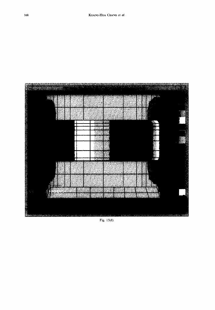
Design sensitivity analysis and results display. The design velocity field and sensitivity coefficients are computed using the boundary displacement method and the direct differentiation method, respectively. Design sensitivity coefficients of stress at element 772 is displayed using color plots. Figure 15(a) shows that, on the front surface, moving design parameter dpl a unit magnitude in the negative Y-direction to make the front side thicker decreases the stress in element 772 by 6078 psi. Design parameter dp2 similarly decreases the stress, but by a lesser amount. The other design parameters are not influential. Figure 15(b) shows that, on the rear surface, perturbing design parameter dp6 a unit magnitude in the positive Y-direction causes the rear surface to be thicker decreasing the stress concentration by 5208 psi. The other design parameters defined on the rear surface similarly decrease the stress, but by a lesser amount. Figure 15(c) shows that design parameter dpl4 has the most influence on the stress performance. Perturbing design parameter dpl4 a unit magnitude in the X-direction makes the upper front slot thicker decreases the stress concentration 19,581 psi. Design parameter dpl5 has the opposite behavior, i.e. moving in the negative X-direction will reduce the stress at element 772. For the rear slot surface, moving the design parameter dpl9 a unit magnitude in the negative X-direction decreases the stress concentration 13,524psi, as shown in Fig. 15(d). The other design parameters defined on the rear slot surface similarly decrease the stress, but by a lesser amount.

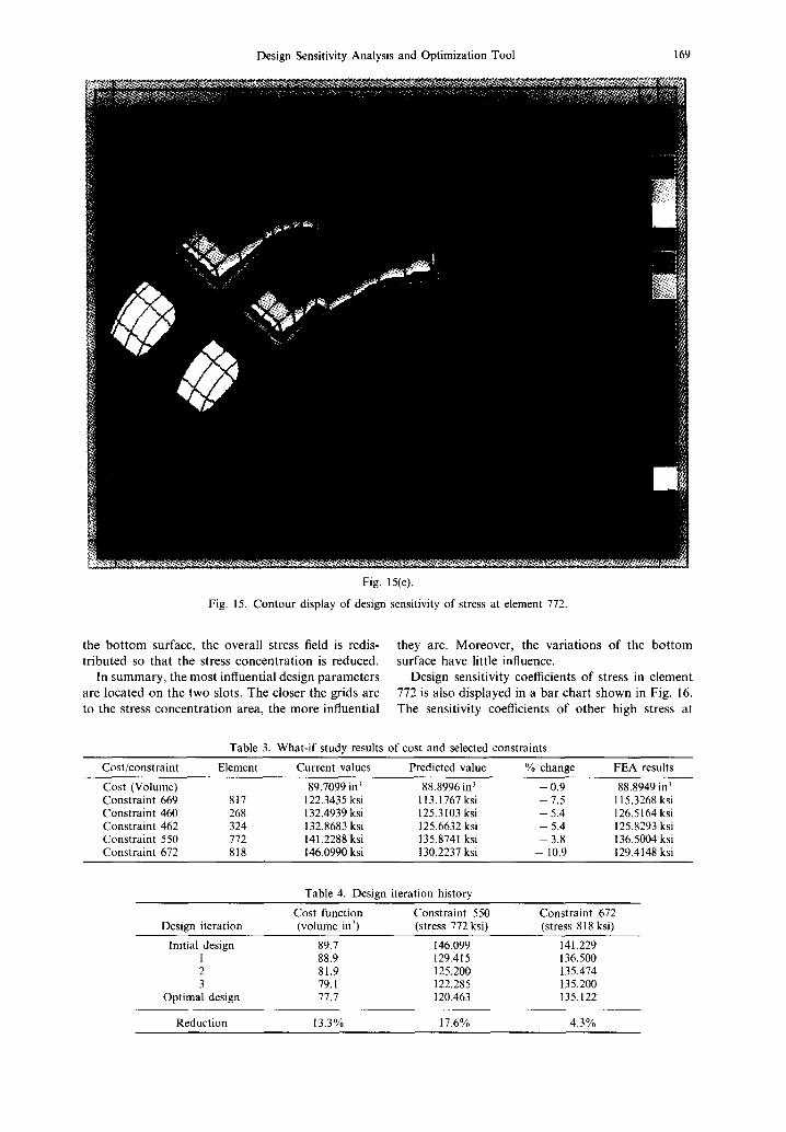
Among the five geometric features, the design perturbations on the bottom surface have the least influence on the stress concentration, as shown in Fig. 15(e). However, the interesting observation is that, instead of adding material to the top surface, moving the grids inward reduces the stress concentration. This is because by cutting out the material on

Table 2. Cost and (selected) constraint function definitions

Cost/constraint Element Current values Upper bound Status

Cost (Volume) 89.7099 in 3 Constraint 669 817 122.3435 ksi 138.75 ksi inactive Constraint 460 268 132.4939 ksi 138.75 ksi inactive Constraint 462 324 132.8683 ksi 138.75 ksi inactive Constraint 550 772 141.2288 ksi 138.75 ksi violated Constraint 672 818 146.0990 ksi 138.75 ksi violated


dpl \ ~ dp2

dp3 ~ ~ ~ ~ dp4

dp6

X ~ dp8 dp9

~ dplO

(b)

J --'L• dpl 5 dp 14

J.L 1 I I 1 II1 I I i1-1111 ~ dp13

' ~ , dpl 1

Y

Z

( c ) Fig. 14(a-c).


II II

dp16 dp17 dp18 dp19 dp20 dp21

l I ¥

I I

I I • I J! I

I Y l ' l I ! Y l y I Y Y

l rrl I I / Z

Y

(d)

dp25 dp24 ~

dp2

(e)

Fig. 14(d and e).

Fig. 14. Design parameterization of the five design boundary surfaces.


Fig. 15(a).

CSk 6,2--D


Fig. 15(b).


Fig. 15(c).

168 KUANG-HUA CHANG e t al.

Fig. 15(d).


Fig. 15(e).

Fig. 15. Contour display of design sensitivity of stress at element 772.

the b o t t o m surface, the overal l s tress field is redis- t r ibu ted so tha t the stress c o n c e n t r a t i o n is reduced.

In s u m m a r y , the m o s t influential des ign p a r a m e t e r s are loca ted on the two slots. The c loser the gr ids are to the stress c o n c e n t r a t i o n area, the m o r e influential

they are. M o r e o v e r , the va r i a t ions o f the b o t t o m surface have little influence.

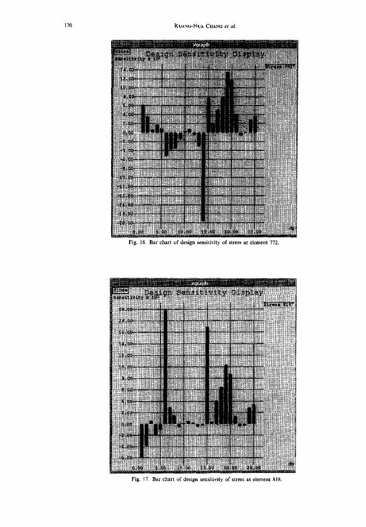
Des ign sensit ivi ty coefficients o f s tress in e l ement 772 is also d i sp layed in a bar cha r t s h o w n in Fig. 16. The sensit ivi ty coefficients o f o t h e r h igh stress at

Table 3. What-if study results of cost and selected constraints

Cost/constraint Element Current values Predicted value % change FEA results

Cost (Volume) 89.7099 in 3 88.8996 in 3 - 0.9 88.8949 in 3 Constraint 669 817 122.3435 ksi 113.1767 ksi - 7.5 115.3268 ksi Constraint 460 268 132.4939 ksi 125.3103 ksi - 5.4 126.5164 ksi Constraint 462 324 132.8683 ksi 125.6632 ksi - 5.4 125.8293 ksi Constraint 550 772 141.2288 ksi 135.8741 ksi - 3.8 136.5004 ksi Constraint 672 818 146.0990 ksi 130.2237 ksi - 10.9 129.4148 ksi

Table 4. Design iteration history

Cost function Constraint 550 Constraint 672 Design iteration (volume in 3) (stress 772 ksi) (stress 818 ksi)

Initial design 89.7 146.099 141.229 1 88.9 129.415 136.500 2 81.9 125.200 135.474 3 79. I 122.285 135.200

Optimal design 77.7 120.463 135.122

Reduction 13.3% 17.6% 4.3%

170 KUANG-HUA CHANG e t al.

® ® ® ®~, ~ @

Fig. 16. Bar chart of design sensitivity of stress at element 772.

Smit~ l l i l ~ m t i ~ l IWi lllWiWim lIIml

NNN @ @ ~ ~ N N N ~ N N N N I N N ~_ N N N N ~ ~ N N N I N

Fig. 17. Bar chart o f design sensitivity of stress at element 818.


t~

o6

172 KUANG-HUA CHANG et al,

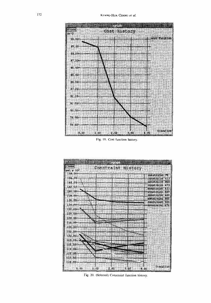
Fig. 19. Cost function history.

Fig. 20. (Selected) Constraint function history.


Dp15 moved Dp14 moved backward

Rear surface forward became thinner

C Material removed from the bottom surface

(a)

ZIz~y ~ ~ / became thinner Material added to the rear slot

(b)

II I I I

Material added to the . . . _ . . _ . . - ~ - ' ~ C Z ~ ~ rear s l o t ~

I Material removed from bottom surface

(c)

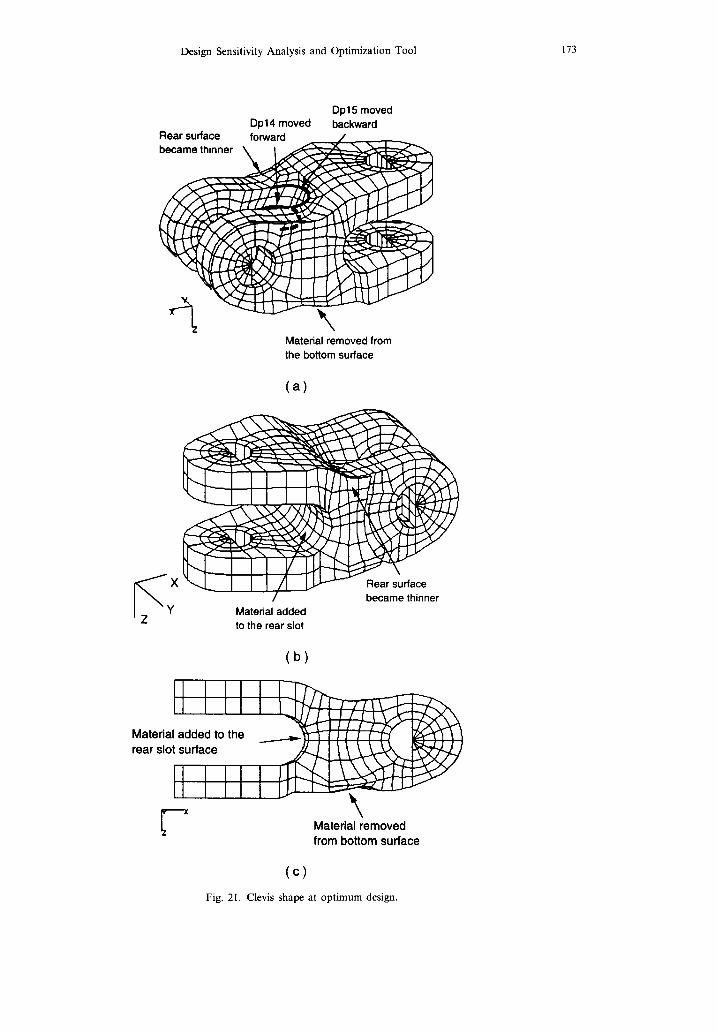
Fig. 21. Clevis shape at optimum design.


".~4 7%.

i

J Fig. 22. Stress contour of clevis at optimum design.

element 818 are displayed in a bar chart shown in Fig. 17. It is found that the steepest descent directions of the two stress constraints are in conflict, e.g., dp6.

Design trade-off and what-if study. Since the design directions for the two high stresses are in conflict, a trade-off study is performed to search for a best design direction using the second option, constraint correction. The design direction is found and a what-if study is performed using the direction and a step size 0.5 in as design perturbation.

Based on the design perturbation, new cost and constraint function values are predicted by DSO using Eq. (22). The results show that stress measures are improved and cost function is reduced by 0.9%, as listed in Table 3. The what-if results shown in the bar chart of Fig. 18 tell that stress in the entire structure is distributed more evenly due to the design change. Note that stress contour of the new design predicted by the DSO can be shown together with the new finite element model using the what-if results display capabilities of the DSO.

Design optimization. Four design iterations are carried out using the interactive design mode, i.e. trade-off and what-if. The design history is summarized in Table 4, and history of cost and selected constraint functions are shown in polygraphs of Figs 19 and 20.

The shape of the clevis at the optimum design is displayed in Fig. 21. As shown in the figures, the rear surface tends to get thinner and the bottom surface tends to move up, which suggest a symmetric design. The front slot tends to become an "S" shape (see from X - Z plane along the positive Y-direction). And no significant changes are found in the front surface and rear slot. The stress contour shown in Fig. 22 tells that the stress concentration at elements 772 and 818 has been relieved and stress near the bottom is increased. However, the increments are not critical. The overall stress distribution over the clevis is more even.

7. CONCLUSIONS

The Design Sensitivity Analysis and Optimization (DSO) tool extended for shape design applications has been presented and demonstrated through examples as a convenient and effective tool to support shape design optimization. The major achievement of the research is integration of geometric modeling, geometric-based shape design parameterization, FEA, error analysis and mesh adaptation, DSA, interactive design method, and optimization using a systematic shape design process to develop a practical and useful tool for shape design applications. One of


the difficulties encountered in the research is that finite element mesh distorts easily due to structural shape changes. The distortion causes inaccurate F E A results or even cast-off by the F E A tool. Currently, the p -FEA method 26 is being investigated to overcome this problem. Another important study involves connecting the shape DSA and optimization to a C A D tool; currently p r o / E N G I N E E R 27 is being investigated. The major challenges involved are the development of a CAD-based design parameterization method and a proper velocity field computat ion method 2° using existing C A D and F E A tools.

Acknowledgements--Research supported by NSF-Army- NASA Industry/University Cooperative Research Center for Simulation and Design Optimization of Mechanical Systems.

REFERENCES

1. R. T. Haftka and R. V. Grandhi, "Structural shape optimization--a survey," Computer Methods in Applied Mechanics and Engineering 57, 91-106 (1986).

2. Y. Ding "Shape optimization of structures--a literature survey," Computers and Structures 24(6), 985-1004 (1986).

3. K. H. Chang, K. K. Choi and J. H. Perng, "Design sensitivity analysis and optimization tool for sizing design applications," Fourth AIAA/AIR Force/NASA/ OAI Symposium on Multidisciplinary Analysis and Optimization, Paper No. 92-4789, Cleveland, Ohio, 21-23 September 1992.

4. J. L. T. Santos and K. K. Choi, "Integrated computational considerations for large scale structural design sensitivity analysis and optimization," GAMM Conference on Discretization Methods and Structural Optimization, University of Siegen, FRG, October 1988.

5. PDA Engineering, Patran Plus User's Manuals. Vols. I and II, Software Products Division, 1560 Brookhollow Drive, Santa Ana, CA, 1987.

6. G. J. DeSalvo and J. A. Swanson, Ansys Engineering Analysis System, User's Manual, Vols I and II, Swanson Analysis Systems, Inc., P.O. Box 65, Houston, PA 15342-0065, 1989.

7. MSC/NASTRAN, MSC/NASTRAN User's Manual, Vols I and II, The MacNeal-Schwendler Co., 815 Colorado Boulevard, Los Angeles, CA 90041, 1988.

8. ABAQUS, ABAQUS User's Manual, The Hibbit, Karlsson & Sorensen, Inc., 100 Medway Street, Providence, RI 02906-4402, 1990.

9. K. H. Chang and K. K. Choi, "An error analysis and mesh adaptation method for shape design of elastic

solids," Computers and Structures 44(6), 1275-1289 (1992).

10. E. J. Haug, K. K. Choi and V. Komkov, Design Sensitivity Analysis of Structural Systems, Academic Press, New York, 1986.

1 h R. T. Haftka and H. M. Adelman, "Recent develop- ments in structural sensitivity analysis," Structural Optimization 57, 137-151 (1990).

12. AEA Industrial Technology, Harwell Laboratory, Oxfordshire, OXll OR.A, U.K.

13. G. N. Vanderplaats and S. R. Hansen, DOT User's Manuel, VMA Engineering, 5960 Mandarin Avenue, Suite F, Goleta, CA 93117, 1990.

14. Open Software Foundation, OSF/Motif Programmer's Guide, Prentice Hall, Englewood Cliffs, NJ 07632, 1988.

15. X Window, X Window System User's Guide, O'Reilly & Associates, CA 95472, 1989.

16. K. K. Choi and K. H. Chang, "Shape design sensitivity analysis and what-if workstation for elastic solids," AIAA 32nd SDM Conference, Paper No. 91-1206, April 1991.

17. K. K. Choi and K. H. Chang, "Shape design sensitivity analysis and optimization of elastic solids," Structural Optimization: Status & Promise: AIAA "Progress in Astronautics and Aeronautics" series (edited by Manohar P. Kamat), 1993.

18. O. C. Zienkiewicz and J. Z. Zhu, "A simple error estimator and adaptive procedure for practical engineering analysis," International Journal for Numerical Methods in Engineering 24, 337-357 (1987).

19. E. Rank and O. C. Zienkiewicz, "A simple error estimator in the finite element method," Communica- tions in Applied Numerical Methods 3, 243-249 (1987).

20. K. K. Choi and K. H. Chang, "A study on velocity field computation for shape design optimization," Journal of Finite Elements in Analysis and Design 15, 317-341 (1994).

21. T. M. Yao and K. K. Choi, "3-D shape optimal design and automatic finite element regridding," International Journal for Numerical Methods in Engineering 28, 369-384 (1989).

22. K. K. Choi and T. M. Yao, "3-D shape modeling and automatic regridding in shape design sensitivity analysis," Sensitivity Analysis in Engineering, NASA Conference Publication 2457, pp. 329-345, 1987.

23. K. H. Chang and K. K. Choi, "A geometry based shape design parameterization method for elastic solids," Methods of Structures and Machines 20, 215-252 (1992).

24. J. S. Arora, Introduction to Optimal Design, McGraw- Hill, New York 1989.

25. S. Peterson and T. A. Stone, "Finite element analysis of M88 tow bar clevis," TACOM Report, 15 May 1987.

26. B. A. Szabo and I. Babuska, Finite Element Analysis, John Wiley, New York 1991.

27. Parametric Technology Corporation. Pro~ENGINEER User's Guide, Release 9.0, Parametric Technology Corporation, Waltham, MA, 1993.

design sensitivity analysis and optimization tool...

Documents