DESIGNING A VISUAL FRONT END IN AUDIO-VISUAL AUTOMATIC SPEECH

RECOGNITION SYSTEM

A Thesis

presented to

the Faculty of California Polytechnic State University,

San Luis Obispo

In Partial Fulfillment

of the Requirements for the Degree

Master of Science in Electrical Engineering

by

Junda Dong

June 2015

ii

© 2015

Junda Dong

ALL RIGHTS RESERVED

iii

COMMITTEE MEMBERSHIP

TITLE: Designing a Visual Front End in Audio-Visual Automatic Speech

Recognition System

AUTHOR: Junda Dong

DATE SUBMITTED: June 2015

COMMITTEE CHAIR: Dr. Xiaozheng (Jane) Zhang, PhD

Professor of Electrical Engineering,

Graduate Coordinator

COMMITTEE MEMBER: Dr. Xiao-Hua (Helen) Yu, PhD

Professor of Electrical Engineering,

COMMITTEE MEMBER: Dr. Wayne Pilkington, PhD

Associate Professor of Electrical Engineering,

iv

ABSTRACT

Designing a Visual Front End in Audio-Visual Automatic Speech Recognition System

Junda Dong

Audio-visual automatic speech recognition (AVASR) is a speech recognition technique

integrating audio and video signals as input. Traditional audio-only speech recognition system

only uses acoustic information from an audio source. However the recognition performance

degrades significantly in acoustically noisy environments. It has been shown that visual

information also can be used to identify speech. To improve the speech recognition performance,

audio-visual automatic speech recognition has been studied. In this paper, we focus on the design

of the visual front end of an AVASR system, which mainly consists of face detection and lip

localization. The front end is built upon the AVICAR database that was recorded in moving

vehicles. Therefore, diverse lighting conditions and poor quality of imagery are the problems we

must overcome.

We first propose the use of the Viola-Jones face detection algorithm that can process

images rapidly with high detection accuracy. When the algorithm is applied to the AVICAR

database, we reach an accuracy of 89% face detection rate. By separately detecting and

integrating the detection results from all different color channels, we further improve the

detection accuracy to 95%. To reliably localize the lips, three algorithms are studied and

compared: the Gabor filter algorithm, the lip enhancement algorithm, and the modified Viola-

Jones algorithm for lip features. Finally, to increase detection rate, a modified Viola-Jones

algorithm and lip enhancement algorithms are cascaded based on the results of three lip

localization methods. Overall, the front end achieves an accuracy of 90% for lip localization.

v

ACKNOWLEDGMENTS

I would like to express my sincere gratitude to my advisor Dr. Xiaozheng (Jane) Zhang,

for her full support, guidance, understanding and encouragement throughout my thesis. Without

her help, my thesis work would not have been to be finished. In addition, I express my

appreciation to Dr. Wayne Pilkington, Dr. Xiao-Hua (Helen) Yu for having served on my

committee and for their suggestions.

Thanks also go to all the faculty of the Electrical Engineering Department at Cal Poly for

expanding my knowledge and improving my abilities. Special thanks go to my friends and

classmates who helped me throughout my whole academic study.

Finally, I would like to thank my parents and uncle's family for their unconditional love

and support during the last two years. I would not have been able to complete this thesis without

their continuous encouragement.

vi

TABLE OF CONTENTS

Page

LIST OF TABLES ..................................................................................................................... viii

LIST OF FIGURES ...................................................................................................................... ix

CHAPTER

1. INTRODUCTION .................................................................................................................... 1

1.1 Background ......................................................................................................................... 1

1.2 Previous Work in this Area ................................................................................................. 4

1.3 Thesis Organization ............................................................................................................ 6

2. FACE DETECTION ................................................................................................................. 7

2.1 Features ............................................................................................................................... 8

2.2 Integral Image ..................................................................................................................... 9

2.3 Learning Classification Functions .................................................................................... 11

2.4 The Attentional Cascade ................................................................................................... 16

2.5 Viola-Jones Algorithm Implementation ........................................................................... 21

3. LIP LOCALIZATION ............................................................................................................ 27

3.1 Gabor Filter ....................................................................................................................... 27

3.1.1 Gabor Filter and Its Properties ................................................................................... 28

3.1.2 Gabor Filter Set .......................................................................................................... 30

3.1.3 Gabor Filtering Algorithm ......................................................................................... 33

3.2 Lip Features Extraction ..................................................................................................... 36

3.3 Lip Gradient Algorithm .................................................................................................... 39

vii

3.3.1 Color-based Gradient .................................................................................................. 39

3.4 Modified Viola-Jones Algorithm for Lip Localization ...................................................... 43

3.5 Final Lip Localization Algorithm ..................................................................................... 45

4. CONCLUSION AND FUTURE WORK ................................................................................ 48

4.1 Front End Performance ...................................................................................................... 48

4.2 Front End Limitations and Future Work ............................................................................ 50

REFERENCES ............................................................................................................................ 52

APPENDICES

A: Matlab Algorithms Code ..................................................................................................... 54

viii

LIST OF TABLES

Table Page

2.1: Results of Viola-Jones face detection ................................................................................... 23

2.2: Results of Viola-Jones face detection in different color spaces ........................................... 26

3.1: Average training set lip measurements ................................................................................. 31

3.2: Results of Gabor filter algorithm for lip localization ........................................................... 38

3.3: Results of lip gradient algorithm for lip localization ............................................................ 43

3.4: Results of modified Viola-Jones algorithm for lip localization ............................................ 45

3.5: Results of cascade algorithm for lip localization .................................................................. 46

4.1: Algorithms performance summary ....................................................................................... 48

4.2: Front end performance summary .......................................................................................... 49

ix

LIST OF FIGURE

Figure Page

1.1: Main processing blocks of an audio-visual automatic speech recognition ............................. 2

1.2: Statistical shape model for ASM ............................................................................................ 4

2.1: Haar-like features .................................................................................................................... 8

2.2: Integral image ......................................................................................................................... 9

2.3: Rectangle feature computation ............................................................................................ 10

2.4: ROC (Receiver Operating Characteristic) curve for the 200-feature classifier .................... 15

2.5: First and second features selected by Adaboost algorithm ................................................... 16

2.6: Schematic depiction of the detection cascade .................................................................. 17

2.7: ROC curve comparing a 200-feature classifier with a ten 20-feature classifier ................... 21

2.8: Unqualified face examples .................................................................................................... 22

2.9: True positive face examples ................................................................................................. 23

2.10: False positive face examples ............................................................................................... 24

2.11: False negative faces examples ............................................................................................ 24

2.12: Positive image and negative image example ...................................................................... 25

2.13: Newly detected face in grayscale (a) and red channel (b) .................................................. 26

3.1: Gabor filter impulse response (real component) ................................................................... 29

3.2: Lip measurement diagram .................................................................................................... 31

3.3: 12-component Gabor filter set .............................................................................................. 33

3.4: Gabor filtering processing block diagram ............................................................................ 34

3.5: Total Gabor filter responses (a) Original RGB images (b) Total Gabor responses (c) Mean

-removed total responses .............................................................................................................. 35

x

3.6: Original image and thresholded image ................................................................................. 36

3.7: (a) Blobs after restrictions and (b) Blobs after closing ......................................................... 38

3.8: (a) True positive, (b) false positive and (c) false negative examples for Gabor filter

algorithm ..................................................................................................................................... 38

3.9: Depict of higher and lower lip contour with pseudo hue and luminance ............................. 40

3.10: (a) Original image, (b) Vertical gradient of and (c) Vertical gradient

.................................................................................................................................... 41

3.11: (a) Thresholded upper lip image, (b) Thresholded lower lip image ................................... 42

3.12: (a) True positive, (b) false positive and (c) false negative examples for lip gradient

algorithm ..................................................................................................................................... 43

3.13: Possible lip bounding boxes examples ............................................................................... 44

3.14: (a) True positive, (b) false positive and (c) false negative examples for Viola-Jones lip

localization algorithm ..................................................................................................................45

3.15: Lip gradient improved examples ........................................................................................ 46

3.16: Cascade lip detection algorithm block diagram .................................................................. 47

1

CHAPTER 1

INTRODUCTION

1.1 Background

Automatic speech recognition (ASR) is a popular research field that can be defined as the

translation of spoken words into text. Automatic speech recognition has made significant

progress in recent years and has been widely used in practical applications like computers,

mobile phones, and tablets with speech recognition function. However, conventional automatic

speech recognition techniques are sensitive to noise. For example if the electronic devices are

used in crowded environments, the recognition is unreliable. To improve recognition

performance in noisy environments, visual speech cues can be used to enhance speech

recognition. Visual speech cues are provided by tracking the lip movement of a speaking person

as they form different speech sounds. It is a very valuable source of speech information that is

not affected by acoustic noise. Researchers widely accept that a key to robust automatic speech

recognition in real world situations is the use of a combination of audio and visual information

[1].

Human speech perception is bimodal in nature. Humans combine auditory and visual

information in deciding what has been spoken, especially in noisy environments [2]. The visual

information's benefit to speech intelligibility in noise has been quantified as far back as in Sumby

and Pollack (1954). They demonstrated that the face of a speaker enhanced the identification of

audio speech in noise. Furthermore, bimodal fusion of audio and visual stimuli in perceiving

speech has been demonstrated by McGurk and MacDonald (1976). For example, when the

2

spoken sound /pa/ is superimposed on the video of a person uttering /ba/, most people perceive

the speaker as uttering the sound /da/. The content spoken by humans can be perceived better by

both audio and visual information.

There are several reasons why visual information benefits automatic speech recognition.

First, it helps recognition systems localize the audio source. Second, it also provides speech

segmental information to supplements the audio speech. Third, it contains complementary

information about the source of articulation. The visibility of articulators, such as the tongue,

teeth and lips, can disambiguate close pronunciations. For example, unvoiced constants /p/ and

/k/, voiced consonant pairs /b/ and /d/, and the nasals /m/ and /n/ are confusable in acoustics as

they are similar in sound. Therefore there has been significant interest in combining audio and

visual information to improve automatic speech recognition.

Figure 1.1: Main processing blocks of an audio-visual automatic speech recognition

Automatic recognition of audio-visual speech introduces new and challenging tasks. The

block-diagram of Figure 1.1 demonstrates the main process of an audio-visual automatic speech

recognition system. In addition to the traditional audio front-end where useful audio features are

extracted, visual features that are informative to speech must be extracted from video of the

speaker’s face. This requires robust face detection, as well as localization and tracking of the

3

speaker’s lips, followed by visual feature extraction. In contrast to audio-only system, there are

now two streams of features available for recognition, one from each modality. The combination

of the audio and visual streams should ensure that the resulting system performance is better than

the best of the two single modalities. Both issues, namely the visual front end design and audio-

visual fusion, constitute difficult problems, and they have generated significant research work by

the scientific community.

As shown in Figure 1.1, audio-visual ASR systems differ from the traditional ASR

system in three main aspects: the visual front end design, the audio-visual integration strategy

and the speech recognition method used. The visual front end of AVASR is composed of two

highly researched parts: face detection, lip localization and tracking. While face detection is

more extensively researched, being able to locate and track the face and lips within any image

frame in any environment poses a challenging task. For this reason, the focus of this thesis is

robust face detection and lip localization based on still images from the AVICAR database. The

AVICAR database was recorded in an automotive environment with different driving speeds by

University of Illinois researchers [22]. There were four cameras on the dash board and seven

microphones on the sun visor. The videos were recorded at 35 mph with windows up or down, or

55 mph with the windows up or down. Generally, the in-car environment can be considered as a

worst-case scenario for ASR. Background noise and mechanical vibrations from traveling

vehicles severely decrease operational signal-to-noise ratios for audio processing. Therefore

incorporating visual speech in this case has the potential to significantly increase the

performance for ASR.

4

1.2 Previous Work in This Area

The visual features used for automatic speech recognition can broadly be divided into

three categories, appearance-based features, shape-based features and joint appearance and shape

features.

In appearance-based feature approach, the image part typically containing the speaker’s

face/lip region is considered as informative for face/lip detection. These regions are the region of

interest. Such regions can be a rectangle containing the mouth, the lower face or the entire face,

according to the detection target. The appearance-based features are typically extracted from the

region of interest (ROI) using image transforms, such as transformation to different color space

components, where pixel values of typical faces/lips are used. Some frequently used transforms

include Principal Component Analysis, Discrete Cosine, Wavelet Transforms and Linear

Discriminant Analysis. The Viola-Jones algorithm is also considered an appearance-based

algorithm where the features used are Haar wavelet in gray scale intensities sequences.

Figure 1.2: Statistical shape model for ASM

In contrast to appearance based features, shape based feature extraction assumes that

most visual speech information is contained in the shape (contour) of the speaker’s face/ lip [2].

Two types of features are within this category: Geometric features, and shape model-based

features. Geometric features are a number of high level features that are extracted from the

faces/lip contour, such as the contour height, width, perimeter, face feature position as well as

5

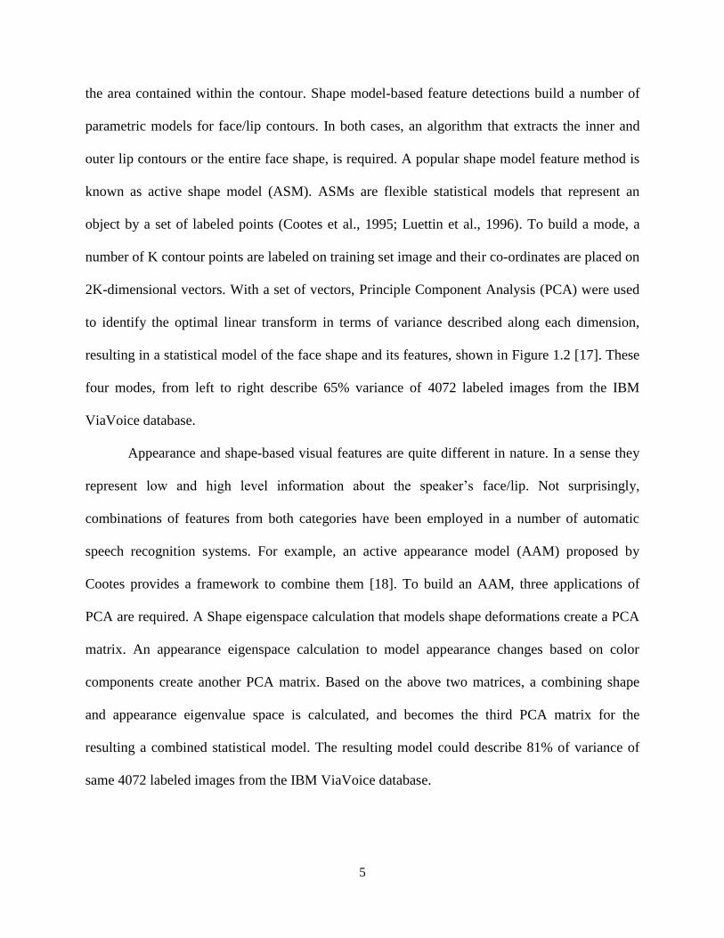
the area contained within the contour. Shape model-based feature detections build a number of

parametric models for face/lip contours. In both cases, an algorithm that extracts the inner and

outer lip contours or the entire face shape, is required. A popular shape model feature method is

known as active shape model (ASM). ASMs are flexible statistical models that represent an

object by a set of labeled points (Cootes et al., 1995; Luettin et al., 1996). To build a mode, a

number of K contour points are labeled on training set image and their co-ordinates are placed on

2K-dimensional vectors. With a set of vectors, Principle Component Analysis (PCA) were used

to identify the optimal linear transform in terms of variance described along each dimension,

resulting in a statistical model of the face shape and its features, shown in Figure 1.2 [17]. These

four modes, from left to right describe 65% variance of 4072 labeled images from the IBM

ViaVoice database.

Appearance and shape-based visual features are quite different in nature. In a sense they

represent low and high level information about the speaker’s face/lip. Not surprisingly,

combinations of features from both categories have been employed in a number of automatic

speech recognition systems. For example, an active appearance model (AAM) proposed by

Cootes provides a framework to combine them [18]. To build an AAM, three applications of

PCA are required. A Shape eigenspace calculation that models shape deformations create a PCA

matrix. An appearance eigenspace calculation to model appearance changes based on color

components create another PCA matrix. Based on the above two matrices, a combining shape

and appearance eigenvalue space is calculated, and becomes the third PCA matrix for the

resulting a combined statistical model. The resulting model could describe 81% of variance of

same 4072 labeled images from the IBM ViaVoice database.

6

The front end system in this paper benefits from previous work by Robert Hursig [15]

and Benefsh Husain [16]. Robert Hursig proposed a shifted HSV color space as the feature space

for face detection and lip localization. Then, the face candidate localization and face model joint

histogram estimation were implemented on sHSV color space to define a face model and

candidate distribution. According to the face model and the candidate distribution, the

Bhattacharyya coefficient was utilized to detect faces. Following the face detection, a Gabor

filter-based lip localization algorithm was developed. For Benefsh Husain's front end, she

implemented a face detection algorithm by cascading Viola-Jones, template matching and Bayes

classifier algorithm. Her lip localization method is the lip enhancement method for hybrid

gradient which was developed as a lip segmentation technique.

1.3 Thesis Organization

This thesis will develop the front end design which contains robust face detection and lip

localization. Chapter 2 will detail the Viola-Jones algorithm and apply it to the AVICAR

database where the RGB color images were captured in the moving vehicles. This chapter will

also include experimental results of using the Viola-Jones algorithm on different color spaces of

same training images. Chapter 3 discusses three different lip localization algorithms: Gabor filter,

color-based algorithm and the modified Viola-Jones algorithm for lip localization, respectively.

Once again testing based on the AVICAR database will be used to justify the effectiveness of the

algorithms developed. Based on results of above three algorithms, the final lip localization

algorithm is built by cascading the modified Viola-Jones and the lip gradient algorithm. Chapter

4 summarizes the front end overall performance for both the face detection and lip localization. It

will discuss the limitation of the algorithms as well as possible future work.

7

CHAPTER 2

FACE DETECTION

As it was briefly mentioned in the introduction, face detection is the first step in the

visual front-end design. In general, robust face detection is quite difficult, especially in a car

environment where face poses, lighting condition and background are changing all the time when

the vehicle is moving. This problem has attracted significant interest in the field of computer

vision. Many face detection methods have been developed, such as color segmentation, Bayes

classifier, template matching, motion information, etc. Some other methods use statistical

modeling techniques, like principal component analysis, active shape model, active appearance

model, linear discriminant analysis, etc. In this work, a popular face detection technique, the

Viola-Jones algorithm, is used to detect faces. The Viola-Jones face detection algorithm is

capable of processing images extremely rapidly while achieving high detection rates [5]. It has

three key contributions, compared with other techniques. The first is the introduction of a new

image representation called the ''Integral Image'' which allows the features to be computed

quickly. The second is a simple and efficient classifier which is built by selecting a small number

of important rectangle features from a large set of rectangle features using the Adaboost learning

algorithm. The third is a method for combining successively more complex classifiers in a

cascade structure which dramatically increases the speed of the detector. We will describe these

in details in subsequent sections.

8

2.1 Features

The processes we use to classify images are based on the value of simple features. There

are many reasons for using features values rather than the raw pixel values directly. One reason

is that features can contain important facial information which is difficult to represent using a

small quantity of pixels. Another critical reason is that a feature-based system operates much

faster than a pixel-based system. To be more specific, we use three kinds of simple features, edge

features, line features and diagonal line features, as shown in Figure 2.1 below. The value of a

two-rectangle feature in (a) and (c), called the edge feature, is the difference between the sum of

the pixel values contained within two rectangular regions. The regions of these rectangles have

the same size and shape and are horizontally or vertically adjacent. In (b) and (d), a three-

rectangle feature called the line feature computes the pixel sum within two outside rectangles and

subtracts it from the sum of pixels in the middle rectangle. The last feature shown in (e), a four-

rectangular feature defined as the diagonal line feature computes the difference between pixel

sums in diagonal pairs of rectangles. If the resolution of the face image is 24×24, the exhaustive

set of rectangle features is very large, more than 160000. There are 43200, 27600, 43200, 27600

and 20736 features of category (a), (b), (c), (d), (e) respectively; hence 162,336 features in all.

(a) (b) (c) (d) (e)

Figure 2.1: Haar-like features

9

2.2 Integral Image

Rectangle features can be computed very rapidly using an intermediate representation for

the image which we call the integral image [3]. The integral image located at x, y which contains

the sum of the pixels above and to the left of x, y, is computed as:

(2.1)

where is the integral image and is the original image, shown in Figure 2.2 below.

Figure 2.2: Integral image

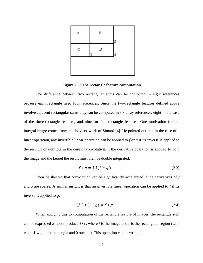
Using the integral image any rectangular sum can be computed in four array references,

shown in Figure 2.3 below. Specifically, using the notation in the below figure 2.3, all the

coordinates below are at the corner of the bottom right rectangles D, then having

, the sum within rectangle D

spanned by A, B, C and D is

(2.2)

Where I(A), I(B), I(C) and I(D) is the integral image of A, B, C and D, respectively.

10

Figure 2.3: The rectangle feature computation

The difference between two rectangular sums can be computed in eight references

because each rectangle need four references. Since the two-rectangle features defined above

involve adjacent rectangular sums they can be computed in six array references, eight in the case

of the three-rectangle features, and nine for four-rectangle features. One motivation for the

integral image comes from the 'boxlets' work of Simard [4]. He pointed out that in the case of a

linear operation, any invertible linear operation can be applied to f or g if its inverse is applied to

the result. For example in the case of convolution, if the derivative operation is applied to both

the image and the kernel the result must then be double integrated:

(2.3)

Then he showed that convolution can be significantly accelerated if the derivatives of f

and g are sparse. A similar insight is that an invertible linear operation can be applied to f if its

inverse is applied to g:

(2.4)

When applying this to computation of the rectangle feature of images, the rectangle sum

can be expressed as a dot product, , where i is the image and r is the rectangular region (with

value 1 within the rectangle and 0 outside). This operation can be written:

11

(2.5)

The integral image is in the double integral of the image (first along rows and then along

columns). The second derivative of rectangle (first in row and then in column) is four delta value

at the corner of the rectangle. Evaluation of the second dot product is accomplished with four

array accesses.

After computation of rectangle features, we generate a very large and varied set of

features. Typically, the number of the features is more than enough to represent the image. This

result set provides features of arbitrary aspect ratio and finely sampled locations. Basically, it

appears as though the set of rectangle features provide a rich image representation which

supports effective learning. The extreme computational efficiency of rectangle features help

compensation for their limitation.

2.3 Learning Classification Functions

After we have a feature set, positive and negative training data, there are several machine

learning approaches which can be used to classify the images. Sung and Poggio use a mixture of

Gaussian model [19], Rowley uses a small set of sample image features and a neural network

[20]. More recently Roth has tried a new and unusual image representation and have used the

Winnow learning procedure [21].

Recall that we have 160,000 rectangle features associated with the sub-window of each

training image, a number much larger than the image pixel number. Even though each feature

can be calculated efficiently, the whole feature set computation is prohibitively expensive. In

Viola and Jones algorithm, according to the experiments, they proposed that a very small number

of features can be combined to form an effective classifier [5]. The main challenge is to find

these small number of features. Then they used a variant of the AdaBoost algorithm both to

12

select the features and to train the classifier. In its original form, the AdaBoost learning

algorithm is used to boost the classifications that combine some weak classifiers to form a strong

one. The combination algorithm is called a weak learner. For example, the perceptron learning

algorithm searches over the set of possible perceptrons and return the perceptron with the lowest

classification error. The learner is called weak because the best classification function still can't

classify the train data well. Usually for a given problem the best perceptron will only classify the

data correctly 51% of the time. In order to enhance the weak learner, it is called upon to solve a

sequence of learning problems. After the first round of classification, the data are re-weighted in

order to emphasize those which were in correctly classified by the previous weak classifier. The

final strong classifier takes the form of a perceptron, a weighted combination of weaker

classifiers followed by a threshold. The guarantee provided by the AdaBoost Algorithm is strong.

Freund and Schapire have proved that the training error of the strong classifier approaches zero

exponentially in the first several rounds [6]. The key insight is that the boost performance is

related the margin of examples, and that Adaboost achieves large margins rapidly.

The original AdaBoost procedure can be considered as a greedy feature selection process.

The general problem of boosting is that the combination of a large set of classification function

need to find a weighted majority vote. For examples, when combining classifiers, a good

classification function needs a large weight to strongly influence the classification result, while

poor functions only need small weights. AdaBoost is an aggressive mechanism for selecting a

small set of good classifiers which nevertheless have significant variety. One practical method

for solving this problem is to restrict the weak learner to the set of classification function each of

which depend on a single feature. The weak learning function is designed to select the single

rectangle feature which best separates the positive and negative examples. For each feature, the

13

weak classifier determines the optimal threshold classification, such that the minimum number of

examples are misclassified. A weak classifier, h(x, f, p, θ), thus consist of a 24×24 sub-window x

of an image, a feature f, a threshold θ and a polarity p indicating the direction of the inequality:

(2.6)

The weak classifier that we use can be viewed as single node decision trees. Such

structures have been called decision stumps in the machine learning paper [6]. To find weak

classifiers, we use decision stump by exhaustive search algorithm below:

Decision Stumps by Exhaustive Search

Input: n training example arranged in ascending order of feature , probabilistic

weights .

Output: the weak classifier threshold t, toggle p, error E and margin M.

Initialization: .

Assume that the number of positive example is l, the number of negative example is m.

Sum up the weights of the positive examples (resp. negative example), whose f-th feature is bigger than the

present threshold:

.

Sum up the weights of the positive examples (resp. negative example), whose f-th feature is smaller than the

present threshold:

.

Set weighted error: +

+

, .

for i=1...n

if , else,

if and , , and .

if ,

. else,

.

if , jump to next iteration.

if , . else,

.

14

In practice, no single feature can accomplish the classification task with low error.

Features which are selected early yield error rates between 0.1 and 0.3 [5]. As the iteration

continues, the task becomes harder. The features selected in the last rounds yield error rates

between 0.4 and 0.5. Here is the AdaBoost algorithm:

The boosting algorithm for learning a query online. T hypotheses are constructed each using a single feature. The

final hypothesis is a weighted linear combination of the T hypotheses where the weights are inversely proportional

to the training errors.

Given example images where where for negative and positive example

respectively.

Initialize weight

for =0,1 respectively, where m and l are number of negative examples, positive

examples respectively.

For t = 1, ..., T:

1. Normalize the weights,

2. Select the best weak classifier with respect to the weight error

3. Define where and are the minimizer of .

4. Update the weights:

Where if example is classified correctly, otherwise, and

.

The final strong classifier is:

Where

15

For the Adaboost learning, Viola and Jones demonstrated some simple results, shown in

the Figure 2.4 below, that a classifier constructed from 200 features would yield [5]. Given a

detection rate of 95%, the classifier yielded a false positive rate of 1 in 14084 on the dataset.

Figure 2.4: ROC (Receiver Operating Characteristic) curve for the 200 feature classifier

For the task of detection, the initial rectangle feature selected by AdaBoost are

meaningful and easily interpreted. The first feature, shown in Figure 2.5 below seems to focus on

the region of eyes where is often darker than nose and cheeks. This feature is quite large,

compared with the sub-window and should be insensitive to size and location of the face. The

second feature is about eye and bridge of nose because eyes should be darker. In summary, the

200 feature classifier provides evidence that a boosted classifier constructed from rectangle

features is an effective technique for face detection.

16

Figure 2.5: First and second features selected by Adaboost algorithm

2.4 The Attentional Cascade

This section describes an algorithm for building a cascade of classifiers which increases

detection performance while reducing computational time. The key reason is that smaller

classifiers can be used in cascade which reject many negative sub-windows while detecting

almost all positive instances. The smaller classifiers are combined by Adaboost algorithm using

less number of weak classifers. Simple classifiers can reject the majority of sub-windows before

more complex classifiers are used to achieve low false positive rates.

The classifiers trained by AdaBoost construct different cascade stages. Starting with a

two-feature classifier, a face detector can obtain low false negatives by setting classifier

threshold. A lower threshold yields higher detection rate and higher false positive rates. Based on

training set, two-feature classifier can detect 100% of face with about 50% false positive rate.

The detection performance of two-feature classifier is far from expectation as a face detection

system. Nevertheless executing some operations with the classifier could reduce the number of

sub-windows:

Evaluate the rectangle feature (requires between 6 and 9 array reference per feature).

Compute the weak classifier for each feature (requires one threshold operation per feature).

Combine the weak classifiers (requires one multiply per feature, an addition and a threshold).

The overall form of the detection process is like a degenerate decision tree, what we call a

''cascade''. As shown in Figure 2.6, a positive result from first classifier triggers the evaluation of

17

a second classifier which has been adjusted to achieve very high detection rates. A positive result

from the second classifier triggers a third one, and so on. A negative outcome at any point would

lead to the rejection of the sub-window. In this structure, the cascade would reject a majority of

sub-windows for any single image. As such, it attempts to reject as many negatives as possible at

early stage. While a positive classifier will trigger the evaluation of every classifier in the

cascade, this is an exceedingly rare. Much like a decision tree, subsequent classifiers are trained

using those examples which pass through all the previous stages. As a result, the second

classifier faces a more difficult task than the first. The more difficult examples faced by deeper

classifiers push the entire receiver operating characteristic (ROC) curve downward. At a given

detection rate, deeper classifiers have correspondingly higher false positive rates.

Figure 2.6: Schematic depiction of the detection cascade

The cascade design structure is driven by higher detection performance. The number of

cascade stages and size of each stage must be sufficient to achieve high detection performance

and low computation. Given a trained cascade of classifier, the false positive rate of each stage is

(2.7)

18

where F is the false positive rate of the cascade classifier, K is the number of classifiers and fi is

the false positive rate of the i-th classifier. . Similarly, The detection rate is

(2.8)

The goal for overall false positive and detection rate, target rates can be achieved for each

classifier in the cascade. For example, a detection rate of 0.9 can be achieved by a 10 stage

classifier if each stage has a detection rate 0.99 ( ). While this detection rate is too

high, it is much easier by the fact that each stage can have a false positive rate of about 30%

( ).

When scanning real images, the cascade will process all the sub-windows until it is

decided that the window is negative, or the window succeeds in each classifier which is labeled

positive. As the simple calculation above, the key measure of each classifier is positive rate, the

proportion of windows which are positive, containing a face. The expected number of features

which are evaluated is:

(2.9)

where N is the expected number of features evaluated, K is the number of classifiers, pi is the

positive rate of the i-th classifier, are the number of features in the i-th classifier.

The overall training process involves two types of tradeoffs. In most cases classifiers with more

features will achieve higher detection rates and lower false positive rates. At the same time

classifiers with more features need more time to compute. Basically, the number of classifier

stages, the number of features of each stage and the threshold of each stage have impact on the

cascade design. Given a target F and D, an optimization framework are traded off in order to

minimize the expected number of features N.

19

In practice the framework of this cascade structure is simple to be built. The user chooses

the maximum false positive rate for and the minimum detection rate for . Each layer of the

cascade is trained by AdaBoost with the number of feature used being increased until the target

detection and false positive rates are met. The rates are determined by testing the current detector

on a positive set. If the overall target false positive rate is not met then another layer is added to

the cascade. The negative set for training subsequent layer is obtained by collecting all false

positive results from the negative examples in the current stage. The more precise algorithm is

below:

The Training Algorithm for building a cascade detector

1. User selects value for f, the maximum acceptable false positive rate per layer and d, the minimum acceptable

detection rate per layer.

2. User selects target overall false positive rate, .

3. P = set of positive examples, N = set of negative examples, = number of features in the i-th classifier.

5.

6. While

-

-

- While

*

* Use P and N to train a classifier with features using AdaBoost.

* Evaluate current cascaded classifier on validation set to determine and .

* Decrease threshold for the i-th classifier until the current cascaded classifier has a detection rate of at least

(this also affect )

- If then evaluate the current cascaded detector on the set of non-face and put any false detections

into the negative set N.

20

In order to explore the cascade approach, two simple detectors were trained by Viola and

Jones: a 200-feature classifier and a cascade ten 20-feature classifiers [5]. The first stage

classifier in the cascade was trained using 5000 faces and 10000 non-face images. The second

stage classifier was trained on same 5000 faces and 5000 false positives of the first classifier.

During the cascade detector training process, the subsequent stage is always trained using the

false positive examples from the previous stage.

The 200-feature classifier was trained on all the same examples as the cascade classifier.

Note that without reference to the cascade classifier, it is difficult to choose good non-face

examples to train the classifier. We can use all possible non-face sub-windows from non-face

examples, but it will make training time impractically long. The cascade classifier is trained

effectively by reducing the non-face training examples. It discards easy examples and focuses on

the hard ones. Figure 2.7 below shows the ROC curves of the two classifiers. The results are

slightly different. However the 200-feature classifier is 10 times slower than the cascade one.

Therefore we choose to use the cascade classifier.

21

Figure 2.7: ROC curve comparing a 200-feature classifier with a ten 20-feature classifier

2.5 Viola-Jones Algorithm Implementation

To implement the Viola-Jones algorithm, Matlab computer vision system toolbox is used.

The built-in function can be used detect face or face features such as mouth, nose, eyes and

upper body. To build the function, the Matlab toolbox uses the trained classifier which was

exported as xml file from OpenCV. The trained cascade consists of 22 stages which were trained

by adaboost algorithm using 5000 positive and 3000 negative examples [7]. The function takes

the following parameters: ClassificationModel, MinSize, MaxSize, ScaleFactor, MergeTheshold.

ClassificationModel is to set a cascade classifier model which could be defined as frontal face,

upper body, eye pair, single eye, mouth or nose model. MinSize and MaxSize are set based on

the object size. For mutiscale object detection, one can choose a suitable scale factor by

ScaleFactor. MergeTheshold is to define detection threshold by the detection targets number.

22

The bounding boxes around the same target object will be merged into one bounding box. To use

the built-in function, one first set up cascade object detector using vision.CascadeObjectDetector

function and define its parameters. Second, use the step function with input image and the

cascade object detector one created to return the bounding boxes.

Figure 2.8: Unqualified face examples

When face detection is applied to AVICAR database, we sampled 707 test images by

random time interval from different videos in the database. The videos we used have recorded 12

different people in vehicles. There are several cases we can't detect faces, shown in Figure 2.8

above. It has been found that when the faces are incomplete/obscured and tilted/rotated too much,

the faces cannot be detected. In Viola and Jones paper [5], it suggests that the face detector can

detect faces that are tilted up to about 15 degrees and rotate about 45 degrees. Therefore, we

choose to discard 86 images that meet the above criteria. Based on the remaining 621 AVICAR

23

test images, the MinSize is set to 100 and MergeThreshold in the function is 4 because there are

four faces in one test image.

Table 2.1: Results of Viola-Jones face detection

Face detection technique True positive rate False positive rate False negative rate

Viola-Jones 557/621=89.69% 13/621=1.45% 51/621=9.18%

As seen in Table 2.1, when face detection is applied to the 621 images, 89% face

detection accuracy is achieved. Examples of true positive results, false positive and false

negative results are contained within Figure 2.9, Figure 2.10 and Figure 2.11, respectively. When

a bounding box contains most of the face with all the face features, it is classified as a true

positive image. If the face features are incomplete or missed in the bounding boxes, it is a false

positive example.

Figure 2.9: True positive face examples

24

Figure 2.10: False positive face example

Figure 2.11: False negative faces examples

25

To improve the face detection based on the Viola Jones algorithm, two methods were

explored. One method is to train a new cascade classifier using the AVICAR database. 450

positive images which are sampled from the AVICAR database and 450 negative images from

the Caltech computer vision database are used as the training set. However, the results of the

cascade classifier is much worse than the built-in classifier which used 5000 positive and 3000

negative faces. The result of the self trained cascade yields a 15.42% true positive rate and 0.08%

false positive rate. We believe that the number of training images we input is not enough for the

classifier to differentiate the face sub-windows and non-face sub-windows.

Figure 2.12: Positive image and negative image example

Another improvement method we explored is to implement the algorithm on different

color component of the same images such as red, green, blue or HSV images and its component

layers. While the original Viola-Jones used gray scale images which converted from RGB

images to perform face detection, addition color spaces are investigated to examine their

effectiveness in face detection. Table 2.2 below shows the results using different color

components. It is found that the red layer has the best performance which has 91.47% true

positive detection rate, outperforming the original Viola Jones results. The table does not include

results with hue and saturation components, because only 20 faces out of 621 images were

26

detected. Figure 2.13 shows the newly detected face example detected using the red layer while

original Viola Jones method failed. The pixel values in grayscale and red images are slightly

different which may cause the cascade structure to classify that the red layer image contains a

face.

(a) (b)

Figure 2.13: Newly detected face in grayscale (a) and red channel (b)

The results of using the green, blue and values components are close to that used in the

original Viola Jones method. From the result face images of above useful color spaces, each

layer detected some face images that the other layers couldn't detect. To increase the detection

accuracy, the newly detected results from different color spaces has been added to the RGB

images results.

Table 2.2: Results of Viola-Jones face detection in different color spaces

Color space True positive rate False positive rate False negative rate

Red 568/621=91.47% 12/621=1.93% 41/621=6.60%

Green 543/621=87.43% 15/621=2.42% 63/621=10.14%

Blue 545/621=87.76% 11/621=1.77% 65/621=10.47%

Value 556/621=89.53% 13/621=2.09% 52/621=8.37%

All color space 587/621=94.52% 16/621=2.58% 18/621=2.90%

27

CHAPTER 3

LIP LOCALIZATION

The next goal of this thesis is to locate lip regions for subsequent audio-video speech

recognition. In this chapter, we develop and implement a lip detection algorithm based on face

images yielded by the face detection in the previous chapter. While accuracy is the main goal of

the algorithm development, emphasis is also placed on speed and memory used since the

AVASR needs to run in real time.

We will discuss three different lip detection algorithms in the following sections. In

section 3.1 we develop Gabor filter to perform the lip localization. In section 3.2 we discuss

different lip enhancement techniques and develop our lip localization algorithm based on color

gradient. In section 3.3 we implementation modified Viola-Jones algorithm to detect lips and

perform operations to isolate the lips. Lastly, in section 3.4 we propose a new method that

combined modified Viola-Jones and lip gradient algorithm for improving performance.

3.1 Gabor Filter

A Gabor filter-based feature space is promoted to detect lips within an image based on

shape. The filtered image will be shown to differentiate facial features effectively, including eyes,

nose, lips and contour of face and help to bound the lip region within a face-classified image.

The following sections will explore the Gabor filter, its properties and its implementation to the

lip localization algorithm.

28

3.1.1 Gabor Filter and Its properties

This section will provide an overview of the Gabor filter and its properties toward facial

feature extraction. The Gabor filter is a linear filter whose impulse response is defined as a

sinusoidal function multiplied by a Gaussian function. The Gabor filter is more effective in

representing natural objects than the impulse or difference of Gaussian (DOG) [9].The Gabor

filter can be defined over any number of dimensions but the 2D-Gabor filter will be the focus of

this work. While the exact definition of the Gabor filter varies, this work’s treatment of the

function is defined via several parameters. These parameters define the size, shape, frequency,

and orientation of the Gabor filter among other characteristics. These parameters and their

descriptions are listed below:

: Width of the Gabor filter mask (pixels)

: Height of the Gabor filter mask (pixels)

Ø : Phase of the sinusoid carrier (radians)

: Digital frequency of the sinusoid (cycles/pixel)

: Sinusoid rotation angle (radians)

: Along-Wave Gaussian envelope normalized scale factor

: Wave-orthogonal Gaussian envelope normalized scale factor

Note the spatial frequency of the filter is listed in polar coordinates as opposed to Cartesian x-

and y-axis frequency components. Given these parameters, one definition of the two-dimensional

complex Gabor filter in the discrete, spatial domain is given by

(3.1)

29

where G is the -by- Gabor filter and is the spatial location within the filter

synonymous with , row and column indexing, respectively. Sharing this definition of the

Gabor filter, the Gabor Filter Toolbox from Kamarainen et al. was used to generate all Gabor

filters within the Matlab environment [8]. Figure 3.1 contains an example Gabor filter with the

stated parameters as visualized in three-dimensions and as a surface and in its two-dimensional

environment. Note that this figure displays only the real component of the filter, which is

complex in nature. Also note that the peak response of the filter is at the mask’s center,

and the counter-clockwise rotation of the two dimensional sinusoid by radians.

Figure 3.1: Gabor filter impulse response (real component)

for

In addition to its sparse representation of natural images, the Gabor filter has several

other attractive properties. Kamaraninen et al. notes that a Gabor filter is invariant to

illumination, rotation, scale, and translation [10]. In an unconstrained environment these Gabor

filter properties make the filter an ideal candidate for detecting facial features.

30

3.1.2 Gabor Filter Set

Besides its definition and invariance properties, the Gabor filter is localized in both the

spatial and frequency domains, making it an attractive form for wavelet analysis. However,

creation of bi-orthogonal Gabor wavelets is time consuming and computationally expensive. In

practice, filter banks consisting of various Gabor filter configurations are constructed, yielding

what is called a “Gabor-space.” It has been posited that this Gabor-space is similar to the

processes which takes place in human’s visual cortex, allowing for rapid recognition of complex

patterns in the visual environment.

Hence, the feature extraction process used in this work will also deploy the use of

multiple Gabor filters to represent facial features of interest. Several studies have successfully

utilized Gabor filter sets of varying parameters to locate facial features. Kim et al. proposed a

'eye model bunch' composed of a total of 40 Gabor filters and classified each pixel’s 40-element

filter response as an eye via complex distance metrics [11]. While being successful, this method

was restricted to vertically oriented faces, requiring a vast training set, and elevated memory

demands and processing time. In fact, a majority of Gabor filter set studies restrict the

application to controlled facial imagery, utilizing rotation and scale dependent comparison

measures and designs [10]. When implementing Gabor filter in AVICAR database, the

measurements of upper lip and lower lip thicknesses and orientation need to be recorded. To

reduce scale dependency, lip measurements were recorded as ratio of the upper lip and lower lip

thickness, and , to the height of facial bounding box, . Lip orientations, , were

measured as the absolute rotation of the mouth axis from horizontal. Refer to Figure 3.2 for a

diagram of these parameters. Across the face training set, the average measurement results are in

31

Table 3.1. With these data, we can create the Gabor filter set to represent the lip region

accurately.

Figure 3.2: Lip measurement diagram

Table 3.1: Average training set lip measurements

Measurement Average Value

Upper Lip Thickness Ratio

0.136

Lower Lip Thickness Ratio

0.065

Lip Orientation ( ) 11.25

In the development of the Gabor filter set, several key simplifications were made to

reduce complexity and variability. First, the size of the Gabor filter was kept square such that the

column x and row y were identical. Moreover, the normalized Gaussian envelop scale factors,

and , were kept unity-valued. Lastly, the sinusoid phase offset, , was fixed at zero. Using the

data from Table 3.1, the remaining key parameters of the Gabor filter set were selected.

Referencing the defining Equation below, the final 12-component Gabor filter set, G, is thus

defined as,

(3.2)

32

Where G is defined in Equation 3.2 and n, t and f are the set indices of the Gabor filter size,

sinusoid angle and digital frequency sets, respectively. It means that the Gabor filter set G is a set

of Gabor filters for every combination of n ,t and f. The orientation angle were selected

because the sinusoid orientation was vertically oriented ( ) and ( ) away

from the vertical. The two frequency value , were chosen such that the half period of the

sinusoid was approximately equal to the average upper and lower lip thickness ratio in Table 3.1

The larger filter size, , was selected for the lip contours. The second filter size, ,

was experimentally selected such that the finer detail of the lip, like the lip corners, were

represented clearer. In addition, the Gabor filter's size, , -by- , was chosen such

that over 80% of the total energy within the filter mask for any value of and . Figure 3.3

displays a sample Gabor filter set for a face region of height . Note the positive and

negative values of the filter which have been mapped to grayscale values.

33

Figure 3.3: 12-component Gabor filter set

3.1.3 Gabor Filtering Algorithm

With the Gabor filter set for lip region, the proper color feature space must be chosen

after the face images have been processed. From Hursig et al, the mean values for lip and

surrounding regions differed by 0.04 within the shifted hue space, 0.05 within the saturation

space and 0.1 within the illumination space [12]. The skin and lip hues are similar in magnitude

Also he mentioned that the hue and saturation values are a function of the illumination value.

Therefore, the value components in shifted HSV space, as the feature space for Gabor filter,

could provide sufficient contrast between lip region and the surrounding face.

34

Figure 3.4: Gabor filtering processing block diagram

As a simple, rotationally invariant lip localization space is required, the multidimensional

Gabor filter set space was reduced to a single dimension. Figure 3.4 contains a block diagram of

the entire Gabor filtering process including this space reduction procedure. First, 12 Gabor filter

responses are generated by performing two-dimensional convolution of the face image value

component V independently with each Gabor filter. Next, all 12 Gabor filter responses are

summarized element by element such that the pixel value at any location within the face is the

sum of each Gabor responses, also called Gabor jets. For the purposes of the block diagram, the

total Gabor response are referred as , which size is , the row and column of the face

image.

Due to the positive and negative valued modes of the Gabor filters, the total response

need to be normalized to the range [0,1] and remapped to stress the maximal and minimal Gabor

jet values. The normalization and remapping procedure is defined below as

(3.3)

35

Let the final normalized and remapped Gabor filter response be defined as , which has

size . An illumination-invariant design demands detection of absolute changes in

achromatic intensity, both from high to low and low to high illumination. Referring to Figure 3.5,

the cross section of lip from chin to the region above lip, the eyebrow and its surrounding region

and the below nose part involves many illumination changes. The light condition also cause such

oscillatory change in the Gabor filter responses.

(a) (b) (c)

Figure 3.5: Total Gabor filter responses

(a) Original RGB images (b) Total Gabor responses (c) Mean-removed total responses

36

As shown above, Figure 3.5 contains sample Gabor filter responses ranging from the total

Gabor responses, , in (a) to the mean-removed responses in (c). Note the contrast facial

features have against the face’s background. Smooth skin surfaces, such as the cheeks, provide

minimal response while the mouth opening, lips, nostrils, eyes, and eyebrows provide much

elevated responses. This phenomenon can be attributed to the spatial transitions in illumination

(both positive and negative) around these features. Also note that the near-vertical edges of the

face provide low responses while the near-horizontal edges, such as the chin region, provide

more noticeable responses. With these positive feature qualities, the final Gabor filter response

will now be used as the preferred feature space for lip localization.

3.2 Lip Features Extraction

As the mean-removed total responses are yielded, the face features, such as eyes, noses

and mouths, usually have strong responses than the other parts. The next step is to isolate the lip

contour from the rest of face by threshold. After testing on the training data which has been

normalized and mean-removed, we consider that the top 85% pixel values at lower half images

contains the lip features we want to extract. The example result image is shown in Figure 3.6

below.

Figure 3.6: Original image and thresholded image

37

Once the thresholded images are obtained, the next step is that we need to find the

bounding box for the lips, and distinguish them from other face features. After testing and

tradeoff based on our face images, we define the following restrictions to detect lip blobs:

a) Orientation: Assuming the lips are horizontal or slightly inclined, we limits the lip orientation

degrees. This help in eliminating any vertically blobs.

b) Blob Area: It is tested through the data that lip area is approximately 3% of the entire face.

Hence, we apply a large area limit and a small area limit to eliminate blob area error.

c) Height to width: This rule is based on general lip shape, the bounding box width is longer then

the height.

d) Geometry position: Based on the fact that the faces are frontal and upright, the mouth position

should be within reasonable range. So the blobs can only exist in the lower half of the image and

in addition, the blobs should be higher than 1/8 of the image from the bottom. The edge of any

blob at lower half image should not contact the image edge. In order to form a entire lip by

combining lip blobs together, we close the blobs by disk. As shown in Figure 3.7, after the

restriction process and morphological operation, the largest blobs is the lip features.

38

(a) (b)

Figure 3.7: (a) Blobs after restrictions and (b) Blobs after closing

(a) (b) (c)

Figure 3.8: (a) True positive, (b) False positive and (c) False negative examples for Gabor

filter algorithm

Table 3.2: Results of Gabor filter algorithm for lip localization

Lip localization technique True positive rate False positive rate False negative rate

Gabor Filter 417/587=71.04% 141/587=24.02% 29/587=4.92%

39

The Gabor filter algorithm gave an accuracy of about 71% in the 587-image test set. Sample

images of true positive, false positive and false negative are contained in Figure 3.8 (a), (b) and

(c), respectively. Most of the failures are due to bad Gabor filter responses that lead to the failure

of the blob analysis. For example, the false positive occurs when the lip blob is connected with

the nose, such as in the top (b) of Figure 3.8; the false positive is yielded when the lip blob is

incomplete, such as in the bottom (b); the false negative happens when the lip blob area is too

small, such as in the (c).

3.3 Lip Gradient Algorithm

Next we explore the usefulness of the gradient information in differentiating between lip

contour and the other facial features. The principle of the gradient algorithm is to detect the

illumination changes between the lips and the skin. For example, if the light source comes from

above, the upper part of the lip is bright whereas the region below is relatively dark. If the light

condition is opposite, the lower lip is bright, the upper region is dark. Therefore if the

illumination changes between the lips and the skin are enhanced, the lip contours can be easily

extracted. In the following, several methods are discussed that provide strong gradient between

the lips and the skin.

3.3.1 Color-Based Gradient

There exist several color gradient spaces for lip contour extraction. Stillittano and Caplier

have used two color gradients for the upper and lower lip contours [13]. The gradient

highlights the upper boundary and highlights lower part. The equations are given by

(3.4)

Where I is the luminance, R and G are red component, green component respectively.

40

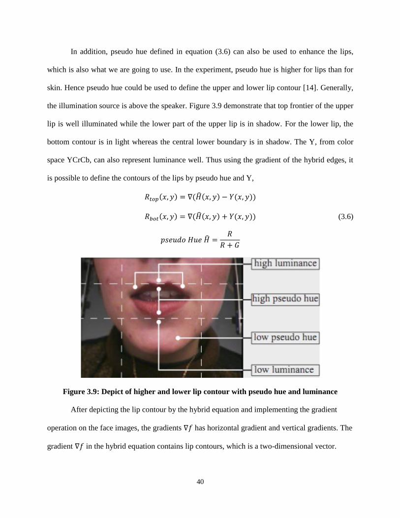
In addition, pseudo hue defined in equation (3.6) can also be used to enhance the lips,

which is also what we are going to use. In the experiment, pseudo hue is higher for lips than for

skin. Hence pseudo hue could be used to define the upper and lower lip contour [14]. Generally,

the illumination source is above the speaker. Figure 3.9 demonstrate that top frontier of the upper

lip is well illuminated while the lower part of the upper lip is in shadow. For the lower lip, the

bottom contour is in light whereas the central lower boundary is in shadow. The Y, from color

space YCrCb, can also represent luminance well. Thus using the gradient of the hybrid edges, it

is possible to define the contours of the lips by pseudo hue and Y,

(3.6)

Figure 3.9: Depict of higher and lower lip contour with pseudo hue and luminance

After depicting the lip contour by the hybrid equation and implementing the gradient

operation on the face images, the gradients has horizontal gradient and vertical gradients. The

gradient in the hybrid equation contains lip contours, which is a two-dimensional vector.

41

(a) (b) (c)

Figure 3.10: (a) Original image, (b) Vertical gradient of and (c) Vertical gradient

of

As shown in Figure 3.10 above, the vertical gradient of the equation highlighted the lips

and other face features in comparison to the rest part of the image. Then, we use thresholds to

convert the gradient image to binary image for classification. After testing the face images in our

database, the pixel values in and are selected to be between -0.25 and 0.37. After using

imtool function in Matlab for mouth region value and testing on the train data, the threshold is

set as below:

(3.7)

42

(a) (b)

Figure 3.11: (a) Thresholded upper lip image, (b) Thresholded lower lip image

Images in Figure 3.11 are obtained by thresholding the image in Figure 3.10. They

contain the upper and lower lip information. After two binary images are merged, we need to

separate out the lip blobs from the other parts of the faces. The images are similar wittoh the

thresholded mean-removed total responses in Gabor filter section. Therefore, the method we

used to separate lip regions and non-lip regions is the same as the blobs analysis in lip feature

extraction in Section 3.1.3.

According to Table 3.3, 75.47% true positive accuracy is achieved when lip gradient

algorithm is applied to 587 test image. It performs better than the Gabor filter algorithm and its

true positive, false positive and false negative examples have been shown in Figure 3.13(a), (b)

and (c), respectively. As with Gabor filter algorithm, errors typically occur where there is little

contrast between the lip pixels and the surrounding pixels when the face is not well lit. Because

the top half lip gradient value is usually larger, only the top half lip is in the bounding such as the

top (b) in Figure 3.13.

43

()

(a) (b) (c)

Figure 3.12: (a) True positive, (b) false positive and (c) false negative examples for lip

gradient algorithm

Table 3.3: Results of lip gradient algorithm for lip localization

Lip localization technique True positive rate False positive rate False negative rate

Lip gradient 443/587=75.47% 135/587=23.00% 9/587=1.53%

3.4 Modified Viola-Jones Algorithm for Lip Localization

Viola-Jones algorithm can be implemented not only for face detection but also for lip

detection. The cascade classifier was trained using the same Viola-Jones face detection training

algorithms which were described in Chapter 2. The difference is that the lip images and the non-

lip images are used as training data. The cascade classifier for mouth has already been trained in

Matlab computer vision toolbox. The implementation of Viola-Jones for lip localization is

similar as face detection. The difference is to set Mouth in ClassificationModel, with no size or

merge threshold limitation.

44

Figure 3.13: Possible lip bounding boxes examples

As shown in Figure 3.14, the built-in function returns the possible bounding boxes which

usually contain eyes, noses, lips and other features that are similar to the mouth region. Therefore

some restrictions are needed to filter out non-lips. The restrictions used here is easier than the

restrictions in section 3.2. Based on lip geometrical information in the test images, the correct lip

bounding boxes should meet the following condition: the bounding box should be located at the

lower half of the image; left edges of bounding boxes are in the left half of image; the bounding

box is the lowest one in all possible boxes. The size of the bounding boxes is from 3% to 15% of

the whole image.

Table 3.4 shows that within 587 detected face images, the proposed lip localization

method succeeded in 92.67% of all detected faces. The results are shown in Figure 3.16(a), (b),

(c) for true positive, false positive and false negative examples, respectively. In most of the false

positive examples, nose was frequently included in the lip region. False negative results occur

when the faces/lips are rotated or when the lighting condition are non ideal.

45

(a) (b) (c)

Figure 3.14: (a) True positive, (b) false positive and (c) false negative examples for Viola-

Jones lip localization algorithm

Table 3.4: Results of modified Viola-Jones algorithm for lip localization

Lip localization technique True positive rate False positive rate False negative rate

Modified Viola-Jones 544/587=92.67% 8/587=1.36% 35/587=5.96%

3.5 Final Lip Localization Algorithm

As demonstrated by the lip localization results in the previous sections, the Viola-Jones

algorithm outperforms other techniques, but some false negative results still remains. Although

the lip enhancement algorithm does not perform as well as the Viola-Jones algorithm and its

processing speed is slow, it is capable of detecting the lips that Viola-Jones misses. Hence, we

combine the two algorithm by first using Viola-Jones algorithm to detect the lips on the face

images. If no lip is found, the lip gradient technique will then be applied to find the lips.

46

Table 3.5 below shows that the final lip localization algorithm is able to improve the

accuracy from 92.67% to 95.4%. The examples that lip gradient algorithm improved are shown

in Figure 3.17. Figure 3.18 demonstrates the flow chart of the final lip localization algorithm.

Figure 3.15: Lip gradient improved examples

Table 3.5: Results of cascade algorithm for lip localization

Lip localization technique True positive rate False positive rate False negative rate

Cascade Algorithm 560/587=95.40% 22/587=3.40% 5/587=1.19%

47

Figure 3.16: Cascade lip detection algorithm block diagram

48

CHAPTER 4

CONCLUSION AND FUTURE WORK

4.1 Front End Performance

The visual front end for AVASR system is built by face detection followed by lip

localization. In face detection, the original Viola-Jones implementation achieved 89.69% true

positive detection rate on RGB color images. With experiments on different color spaces and the

combined algorithm, the detection accuracy has been improved to 95.01%. In lip localization,

three different algorithms have been implemented and compared. Finally, a cascade lip

localization algorithm is built by applying a modified Viola-Jones algorithm followed by lip

gradient algorithm and achieved a total accuracy of 95.4%. Combined with the face detection

results, the overall system is able to accurately locate lips in 90.18% of the images.

As can be seen in Table 4.1, face detection and lip localization algorithm are evaluated

for both the runtime and detection rates. Comparing to the Viola-Jones lip localization algorithm,

Gabor filter and lip gradient algorithm have lower detection rates with 70.68% and 75.08%,

respectively. Also their false positive rates exceeded 20%, whereas a modified Viola-Jones

implementation remains only a 1.86% error rate.

Table 4.1: Algorithms performance summary

Algorithm Runtime* True positive

rate

False positive

rate

False negative

rate

Viola-Jones face detection 0.053 s 94.52% 2.58% 2.90%

Gabor filter 0.163 s 71.04% 24.02% 4.92%

Lip gradient 0.412 s 75.47% 23.00% 1.53%

Viola-Jones lip localization 0.076 s 92.67% 1.36% 5.96%

*per input image as preformed on a Windows 8, 64-bit, core i7 with 4GB RAM

49

The overall front end performance and its comparison to the two previously developed

systems are summarized in Table 4.2. Note that face detection and lip localization results are

based on 621 images within the AVICAR database throughout this thesis. As seen in previous

sections, face detection accuracy is 94.52% which is 587 out of 621 images; cascade lip

localization algorithm achieves 95.4% detection rate, 560 out of 587. We first use Viola-Jones

algorithm for lip localization, then implement lip gradient algorithm on the false negative results

to enhance the detection rate. Relative to previous thesis work, the overall detection rate, 90.18%,

is better than the front end built by Benafsh which has an overall accuracy of 82.21% [16] and

also exceeds the lip localization rate of 75.6%, achieved by Husig [15].

Table 4.2: Front end performance summary

Front End Total runtime Overall Accuracy

Robert Hursig front end 1.760 s 75.6%

Benafsh Husain front end / * 82.32%

Final front end 0.231 s 90.18%

* The total runtime of Benafsh Husain front end was not reported in the paper

The total front end processing time in Matlab environment are shown in Table 4.2. The

processing time has also been improved from Hursig's 1.76s to 0.231s per frame. The runtime of

the system built by Benafsh was not clarified in the paper. Based on her front end algorithms as

described in Chapter 1, the runtime should be longer than the front end in this paper. The use of

the Viola-Jones algorithm reduces the time needed for face detection. After the cascade classifier

is trained, Matlab only needs to compute larger quantity of Haar-like features and pass through

the cascade structure. The process to train the cascade classifier is the only time consuming task

but it is trained only once. After the training process is complete, the cascade classifier can be

used on any images for object detection. In Hursig's and Benafsh's front ends, the time

consuming process such as Gabor filtering and gradient evaluation need to be performed for each

and every frame.

50

4.2 Front End Limitations and Future Work

Based on the performance of face detection within the AVICAR database, Viola-Jones

face detection is suitable for well aligned faces as described in chapter 2. The rotation and tilt of

the face will cause the detection to be unreliable. We also notice that the occluded or incomplete

faces will not be detected. For example, if the eyes are obstructed or part of the face is blocked,

the face detection will usually fail. Moreover, harsh backlighting may cause failures. For

example, when the faces are dark while the background is relatively light, the algorithm can't

reliably detect the faces. The improvement in the future for Viola-Jones algorithm is to add more

rectangle features. Besides the five traditional Haar-like features, we can rotate the original

features by 45 degrees; the rectangles in the features could also be of different sizes. Another

improvement method is to train a more complete cascade classifier. When training a cascade

structure, we could add more positive images with rotated or tilted faces to the training data.

From the lip localization results, Gabor filter and lip gradient technique don't perform

well due to several reasons. The image quality and lighting condition are the main reasons for

lower detection accuracy. If the lighting is too dark, Gabor filtering doesn't have strong

responses and the lip gradient algorithm does not have strong illumination changes, leading to

small responses in lip regions. If the face is only partially lit, the detection will fail. In harsh

imaging conditions, the resulting bounding boxes would typically contain both nose and lip or

sometimes only nose. Threshold value is yet another problem. In work by Husain, several

parameters such as the threshold for upper and bottom lip gradient are employed to be 0.028 and

0.03. The threshold for Gabor filter algorithm in this work is chosen according to the top 15%

value. These parameters need to be tuned based on lip localization results and are not suitable for

all test images. One has to tradeoff some test images to achieve higher detection rate. In the blob

51

analysis, the similar problem comes again. The restrictions in the blob analysis could discard

most of the non-lip blobs, but not all of them. The nose parts usually remain after the blob

analysis and then cause the false positive detection because it's located just above the mouth and

it has a strong filtered response or gradient value. It is difficult to set restrictions which only keep

lip blobs. Based on evaluation of 587 test images, Gabor filter and lip gradient algorithm

achieves 70% and 75% accuracy, respectively. Based on above two algorithm performance,

neither of them have either good filtered responses or strong gradients. Gabor filter algorithm is

based on filter shape and color space; lip gradient algorithm is based on color space. For

AVICAR database, the condition for lip localization is very difficult, there are too many

unconstrained factors. The Gabor filter bank and color space of this work is impossible to adapt

to variations in all face images.

In future work, the visual front end can be built based on the videos in the AVICAR

database by exploiting temporal information. With accurately detected lips, audio-visual fusion

and speech recognition can then be developed to achieve AVASR.

52

REFERENCES

[1] R. Goecke, "Audio-Video Automatic Speech Recognition: An Example of Improved

Performance through Multimodal Sensor Input," NICTA-HCSNet Multimodal User

Ineraction Workshop, Sydney, Australia, 2005.

[2] G. Potamianos, J. Luettin, I. Matthews, "Audio-Visual Automatic Speech Recognition:

An Overview," Issues in Visual and Audio-Visual Speech Processing, MIT Press, Ch 10,

2004.

[3] F. Crow, "Summed-area Tables for Texture Mapping," Proceedings of SIGGRAPH,

1984, pp. 207-212.

[4] P.Y. Saimard, L. Bottou, P. Haffner, Y. LeCun, "Boxlets: A Fast Convolution Algorithm

for Signal Processing and Neural Networks," Advances in Neural Information

Processing System, vol. 11, pp.571-577.

[5] P.Viola, M. Jones, "Robust Real-Time Face Detection," International Journal of

Computer Vision 57(2), 2004, pp.137-154

[6] Y. Freund, R.E. Schapire, "A Decision Theoretic Generalization of On-line Learning and

An Application to Boosting," Computational Learning Theory: Eurocoly 95, 1995,

pp.23-37.

[7] R. Lienhart, A. Kuranov, V. Pisarevsky, "Empirical Analysis of Detection Cascades of

Boosted Classifiers for Rapid Object Detection," Proceedings of the 25th DAGM

symposium on Pattern Recognition, Magdeburg, Germany, 2003.

[8] J. Kamarainen, V.kyrki, The Gabor Feature in Signal and Image Processing Toolbox,

March 3, 2003.

[9] R. Navarro, A Tebernero, G. Cristobal, "Image Representation with Gabor Wavelets and

Its Applications," Advances in Imaging and electron Physics, Orlando, Academic Press

Inc.

[10] J. Kamarainen, V.kyrki, "Invariance Properties of Gabor Filter-Based Features-Overview

and Applications," IEEE Transaction on Image Processing, vol.15, no. 5, May 2006, pp.

1088-1099.

53

[11] S. Kim, S. Chung, S. Jung, D. Oh, J. Kim, S. Cho, "Multi-Scale Gabor Feature Based

Localization," Proceeding of World Academic of Science, Engineering and Technology,

vol. 21, January 2007, pp. 483-487.

[12] B. Crow, H.A. Montoya, X. Zhang, "Finding Lips in Unconstrained Imagery for

Improved Automatic Speech Recognition", Proceedings of the 9th International

Conference on Visual Information System, Shanghai, China June, 2008

[13] S. Stillittano, A. Caplier, "Inner lip segmentation by combining active contours and

parametric models," Proceeding of the 3rd International Conference on Computer

Vision Theory and Applications, Madeira, Portugal, Junuary, 2008

[14] N. Eveno, A. Caplier, P.Y. Coulon, "A parametric model for realistic lip segmentation,"

Control, Automation, Robotics and Visions, vol. 3, December 2002, pp. 1426-1431

[15] R. Hursig, "Robust unconstrained face detection and lip localization Algorithm Using

Gabor Filters," Master's Thesis, California Polytechnic State University, 2009

[16] B. Husain, "Face Detection and lip localization," Master's Thesis, California Polytechnic

State University, 2011

[17] T.F. Cootes, C.J. Cooper, J. Graham, "Active Shape Models-Their Training and

Application," Computer Vision and Image Understanding, 61(1):38-59, 1995

[18] T.F. Cootes, G.J Taylor, "Active Appearance models," Proceeding of European

Conference on Computer Vision, Freiburg, Germant, 1998, pp484-498.

[19] K. Sung, T. Poggio, "Example-based Learning for View-based Face Detection," IEEE

Patt. Anal. Mach. Intell, 20:39-51, 1998

[20] H. Rowley, S. Baluja, T. Kanade, "Neural Network-based Face Detection," IEEE Patt.

Anal. Mach. Intell, 20:22-38, 1998

[21] D. Roth, M. Yang, N. Ahuja, "A Snowbased Face Detector," Neural Information

Processing 12, 2000

[22] AVICAR Project: Audio-Visual Speech Recognition in a car, 2003-2004, Available

Online: http://www.isle.illinois.edu/sst/AVICAR/

54

APPENDICES

A: MATLAB Algorithms Code

1: Viola-Jones Face Detection function face_number = facedetect(directory) %----------------------------------------------------------------------------

-------- % %Purpose: This function is used to detect face using Viola-Jones object

detection %Input: The directory where the original JEPG image are stored % for example: 'c:\results' %Output: The face number detected % The face images in \faces % The runtime %Author: Junda Dong %Date: Junuary, 2015 %----------------------------------------------------------------------------

--------

dir_name = char(directory); file = dir ( strcat(dir_name, '\*.jpeg')); mkdir('results\faces') face_number = 0; none = 0; file = dir('results\*.jpeg'); tic for n = 1:length(file) filename = strcat('results\',num2str(n),'.JPEG'); I = imread(filename); HSV_I = rgb2hsv(I); facedetector = vision.CascadeObjectDetector('FrontalFaceCART'); facedetector.MinSize = [100, 100]; facedetector.MergeThreshold = 4; fboxes = step(facedetector, I); n_f = size(fboxes,1); boxsize(1,1)= size(fboxes,1); if size(fboxes,1)==0 none = none + 1; end if n_f < 4 Rfboxes = step(facedetector, I(:,:,1)); boxsize(2,1)= size(Rfboxes,1); Gfboxes = step(facedetector, I(:,:,2)); boxsize(5,1)= size(Gfboxes,1); Bfboxes = step(facedetector, I(:,:,3)); boxsize(4,1)= size(Bfboxes,1); release(facedetector); Vfboxes = step(facedetector, HSV_I(:,:,3)); boxsize(3,1)= size(Vfboxes,1); index = find(boxsize == max(boxsize)); switch index(1)

55

case 1 fboxes = fboxes; case 2 fboxes = Rfboxes; case 3 fboxes = Vfboxes; case 4 fboxes = Bfboxes; case 5 fboxes = Gfboxes; end end IFaces = insertObjectAnnotation(I, 'rectangle', fboxes, 'face'); for m = 1:size(fboxes,1) face_name =

strcat('results\faces\',num2str(n),'_',num2str(m),'.JPEG'); face =

I(fboxes(m,2):fboxes(m,2)+fboxes(m,3),fboxes(m,1):fboxes(m,1)+fboxes(m,3),:); imwrite(face, face_name); face_number = face_number+1; end % figure, % imshow(IFaces), % title('Detected faces'); end toc

2: Gabor Filter Lip Detection

%---------------------------------------------------------------------------- % %PURPOSE: This function apply the Gabor Filter to the image, then threshold % total Gabor filter response and extract lip feature by Blob

analysis. %INPUT: RGB face images %OUTPUT: Cropped lip Images %AUTHOR: Junda Dong %DATE: February, 2015 %---------------------------------------------------------------------------

clc; clear all; close all;

tic file = dir('results\faces\*.jpeg'); for n = 1 :length(file

face = imread(['results\faces\' file(n).name]); Image = file(n).name;

% Color Space R = face(:,:,1); G = face(:,:,2); YCRCB = rgb2ycbcr(face); Y = double(YCRCB(:,:,1));

56

pH = double(R)./(double(R)+double(G)); pH(isnan(pH))=0; Ynorm = Y./ max(max(Y)); outimg = pH - double(Ynorm); HSV3 = rgb2hsv(face);

% Gabor Filter Bunch Parameters M=size(HSV3,1); N=size(HSV3,2); sf = 4; theta=[3*pi/8, pi/2, 5*pi/8]; N_gf=floor(sf*M*[1,2]/32); fund=[1 2]; gamma = 1; eta = 1; resp_tot3 = zeros(M,N);

%Perform Filtering Over Each Theta,Frequency Combination for t=1:length(theta) for f=1:length(fund) for k=1:length(N_gf) freq = sf*fund(f)/N_gf(k); g = gfcreatefilter2(freq,theta(t),gamma,eta,N_gf(k)); resp = imfilter(HSV3(:,:,3),g,'corr', 'same'); resp_tot = resp_tot+resp; end end end

%Normalize (Valid) Total Response [Mp, Np] = size(resp_tot); range = [min(min(resp_tot)),max(max(resp_tot))]; resp_tot=(resp_tot-range(1))/(range(2)-range(1)); resp_tot=abs(resp_tot); resp_avg = sum(sum(resp_tot))/(Mp*Np); resp_mr = resp_tot.*(resp_tot>resp_avg);

% Lip Features Extract I = imhist(resp_mr(M/2:M,1:M)); I1 = sort(I,'descend'); for j = 1:256 if sum(I1(1:j,1)) < 0.87 * sum(I) a = j; end end thre = (find(I==I1(a,1))-1)/255; bw = im2bw(resp_mr, thre(1,:)); se = strel('line',1,90); bw1 = imopen(bw,se); bwout = restrMask(bw1); se = strel('disk',2); closeBW = imclose(bwout,se); L = bwlabel(closeBW); s = regionprops(L, 'all'); bdbox = cat(1, s.BoundingBox); imarea = cat(1,s.Area);

57

maxarea = find(imarea == max(imarea)); filename_lip = strcat('results\gabor1\lip_', num2str(n),'.JPEG'); if (~isempty(bdbox)) crop = imcrop(face,bdbox(maxarea,:)); imwrite(crop,filename_lip); else imwrite(face,strcat('results\gabor1\fail_', num2str(n),'.JPEG')); end

figure, imshow(face); rectangle('Position',bdbox(maxarea,:),'EdgeColor','b'); end toc

3: Gabor Filter Toolbox function g = gfcreatefilter2(f0,theta,gamma,eta,n,varargin) % GFCREATEFILTER2 Create normalized 2-D Gabor filter in the spatial domain. % % G = GFCREATEFILTER2(F0,THETA,GAMMA,ETA,N,...) creates a % two-dimensional normalized Gabor filter G with frequency F0, % orientation THETA, normalized width GAMMA along the wave, % normalized width ETA orthogonal to the wave, and size N. % If N is a scalar, G will have equal number of rows and % columns. Also a two element vector N=[NX NY] can be used to % specify the size. % % G = GFCREATEFILTER2(...,'PF',PF) determines that at least % P percent of the Gaussian envelope of the filter must be % included in the filter in frequency domain. For default, % PF=0.998. % % G = GFCREATEFILTER2(...,'PT',PT) determines that at least % P percent of the Gaussian envelope of the filter must be % included in the filter in spatial domain. For default, % PT=0.998. % % Examples % % See also GFCREATEFILTERF2, GFCHECKFILTER2, GFCREATEFILTERF. % % References: % [1] Kamarainen, J.-K., Kyrki, V., Kalviainen, H., Gabor % Features for Invariant Object Recognition, Research % report 79, Department of Information Technology, % Lappeenranta University of Technology % % Author(s): % Joni Kamarainen <Joni.Kamarainen@lut.fi> % Ville Kyrki <Ville.Kyrki@lut.fi> % % Copyright: % % The Gabor Features in Signal and Image Processing Toolbox is % Copyright (C) 2000 by Joni Kamarainen and Ville Kyrki.

58

% % % $Name: V_0_4 $ $Revision: 1.9 $ $Date: 2003/03/03 10:51:17 $ %

pt=0.998; % corresponds approximately to (1-1/512) pf=0.998; if mod(length(varargin),2)>0, error('Each parameter must be given a value.'); end; currentarg=1; while length(varargin)>currentarg, [param,value]=deal(varargin{currentarg:currentarg+1});

switch lower(param) case 'pt' pt=value; otherwise error(['Unknown parameter ''' param '''.']); end; currentarg=currentarg+2; end;

alpha=f0/gamma; beta=f0/eta; if length(n)>1, nx=n(1); ny=n(2); else nx=n; ny=n; end;

% Parittomalla pituudella indeksit -(n-1)/2:(n-1)/2 % Parillisella -(n/2):(n/2-1) % Esim. 9 -> -4:4, 8 -> -4:3 if mod(nx,2)>0, tx=-((nx-1)/2):(nx-1)/2; else tx=-(nx/2):(nx/2-1); end; if mod(ny,2)>0, ty=-((ny-1)/2):(ny-1)/2; else ty=-(ny/2):(ny/2-1); end; [X,Y]=meshgrid(tx,ty); g=abs(alpha*beta)/pi*exp(-alpha^2*(X*cos(theta)+Y*sin(theta)).^2-... beta^2*(-X*sin(theta)+Y*cos(theta)).^2 +... j*2*pi*f0*(X*cos(theta)+Y*sin(theta)));

4: Blob Analysis

function outMask = restrMask(bw) %----------------------------------------------------------------------

59

% %PURPOSE: This program apply the constraints to choose lips blob area %INPUT: The thresholded image containing lip blobs %OUTPUT: The binary image with lip area %AUTHOR: Junda Dong %DATE: February, 2015 %----------------------------------------------------------------------

L = bwlabel(bw); s = regionprops(L, 'all'); bdbox = cat(1, s.BoundingBox); orent = cat(1, s.Orientation); imarea = cat(1, s.Area); orthl = -30; orthr = 30; Siz = size(bw); outLipsMaskd = zeros(Siz); TotArea = double(Siz(1)*Siz(2)); for k=1:1:size(bdbox,1) bwcrop = imcrop(bw,bdbox(k,:)); bwcropMir = fliplr(bwcrop); overlap = bwcrop & bwcropMir; if (orent(k)>= orthl) && (orent(k)<= orthr) && ... (imarea(k)/TotArea < 0.03) && (bdbox(k,4)< bdbox(k,3)) &&... (imarea(k)/TotArea > 0.002) && (bdbox(k,2)> Siz(1)*1/2) &&... (bdbox(k,2)< (Siz(1)-Siz(1)/8)) && (bdbox(k,1)<Siz(2)*1/2) for a = round(bdbox(k,1)):1:(round(bdbox(k,1))+bdbox(k,3)) for b = round(bdbox(k,2)):1:(round(bdbox(k,2))+bdbox(k,4)) if (b <= Siz(1))&& (a <= Siz(2)) outLipsMaskd(b,a) = bw(b,a); end end end end end outMask = (outLipsMaskd > 0); end

5: Lip Gradient %---------------------------------------------------------------------- % %PURPOSE: This program extract the lip features using lip gradients %INPUT: The face JPEG images %OUTPUT: The cropped lip images %AUTHOR: Junda Dong %DATE: February, 2015 %---------------------------------------------------------------------- clc; clear all; close all;

tic file = dir('results\faces\*.jpeg'); for n = 1: length(file) face = imread(['results\faces\' file(n).name]);

60

Totarea = size(face,1)*size(face,2); Image = file(n).name; [result1, gXt, gYt] = gradHnL(face); [result2, gXb, gYb]= gradHnLlow(face);

%Threshold top and bottom vertical grdient gradtht = im2bw(gYt,0.028); gradthb = im2bw(gYb,0.03); gradth = gradtht|gradthb; se = strel('line',1,90); bw = imopen(gradtht,se); bw1 = imopen(gradthb,se); outLipsMaskdb = restrMask(bw1); outLipsMaskdt = restrMask(bw); outLipsMaskd = outLipsMaskdb | outLipsMaskdt; se = strel('disk',2); closeBW = imclose(outLipsMaskd,se); L = bwlabel(closeBW); s = regionprops(L, 'all'); bdbox = cat(1, s.BoundingBox); imarea = cat(1,s.Area); maxarea = find(imarea == max(imarea)); filename_lip = strcat('results\gradient1\lip_', num2str(n),'.JPEG'); if (~isempty(bdbox)) crop = imcrop(face,bdbox(maxarea,:)); imwrite(crop,filename_lip); delete (strcat('results\gradient1\fail_', num2str(n),'.JPEG')); else imwrite(face, strcat('results\gradient1\fail_',num2str(n),'.JPEG')); continue end end toc

function [outimg, gX, gY] = gradHnL(inimg) %---------------------------------------------------------------------- %PURPOSE: This program creates the gradient after the algorithm % emphasizing upper lips %INPUT: RGB Image %OUTPUT: The gradient after the algorithm emphasizing upper lips %AUTHOR: Benafsh Husain, Cal Poly San Luis Obispo %DATE: August 1, 2011 %----------------------------------------------------------------------

R = inimg(:,:,1); G = inimg(:,:,2); YCRCB = rgb2ycbcr(inimg); Y = double(YCRCB(:,:,1)); pH = double(R)./(double(R)+double(G)); pH(isnan(pH))=0; Ynorm = Y./ max(max(Y)); outimg = pH - double(Ynorm); [gX, gY] = gradient(outimg); end

61

function [outimg, gX, gY]= gradHnLlow(inimg) %---------------------------------------------------------------------- %PURPOSE: This program creates the gradient after the algorithm % emphasizing lower lips %INPUT: RGB Image %OUTPUT: The gradient after the algorithm emphasizing lower lips %AUTHOR: Benafsh Husain, Cal Poly San Luis Obispo %DATE: August 1, 2011 %----------------------------------------------------------------------

R = inimg(:,:,1); G = inimg(:,:,2); YCRCB = rgb2ycbcr(inimg); Y = double(YCRCB(:,:,1)); pH = double(R)./(double(R)+double(G)); pH(isnan(pH))=0; Ynorm = Y./ max(max(Y)); outimg = pH + double(Ynorm); [gX, gY] = gradient(outimg); end

5: Viola-Jones Lip Localization function lip_number = lipdetect(directory) %---------------------------------------------------------------------------- % %Purpose: This function is used to localize lips using Viola-Jones object

detection %Input: The directory where the face JEPG images are stored % for example: 'c:\results' %Output: The lip number detected % The lip images in \lips % The runtime %Author: Junda Dong %Date: Feburary, 2015 %----------------------------------------------------------------------------

dir_name = char(directory); file = dir ( strcat(dir_name, '\*.jpeg')); mkdir('results\lips') none = 0; face_number = 0;

tic file = dir('results\faces\*.jpeg'); for n = 1:length(file) face = imread(['results\faces\' file(n).name]); lipdetector = vision.CascadeObjectDetector('Mouth'); lboxes = step(lipdetector, face); Ilips = insertObjectAnnotation(face, 'rectangle', lboxes, 'facefeature'); Totarea = size(face,1)*size(face,2); length = 0; mid = 100;

%Set constrains for lip bounding box for m = 1:size(lboxes,1)

62

if (lboxes(m,2) > size(face,1)*(1/2)) && lboxes(m,1) < size(face,2)/2

&& lboxes(m,2)+lboxes(m,4) > length &&... (lboxes(m,3)*lboxes(m,4))/Totarea < 0.15 &&

(lboxes(m,3)*lboxes(m,4))/Totarea > 0.04 length = lboxes(m,2)+lboxes(m,4); b = m; end end filename_lip = strcat('results\viola-jones1\lip_', num2str(n),'.JPEG'); if (~isempty(lboxes)&& b~=0) crop = imcrop(face,lboxes(b,:)); imwrite(crop,filename_lip); delete (strcat('results\viola-jones1\fail_', num2str(n),'.JPEG')); else imwrite(face,strcat('results\viola-jones1\fail_',num2str(n),'.JPEG')); continue end

figure, imshow(Ilips), title('Detected lips'); figure, imshow(face) rectangle('Position',lboxes(b,:),'EdgeColor','b'); b = 0; end toc