designing an equalizer structure using gradient descent...

DESIGNING AN EQUALIZER STRUCTURE USING

GRADIENT DESCENT ALGORITHMS

A THESIS SUBMITTED IN PARTIAL FULFILLMENT OF THE REQUIREMENTS FOR

THE DEGREE OF

Master of Technology

In

Electronics System and Communication

By

B. PAVAN KUMAR

Department of Electrical Engineering

National Institute of Technology

Rourkela

2007

DESIGNING AN EQUALIZER STRUCTURE USING

GRADIENT DESCENT ALGORITHMS

A THESIS SUBMITTED IN PARTIAL FULFILLMENT OF THE REQUIREMENTS FOR

THE DEGREE OF

Master of Technology

In

Electronics System and Communication

By

B. PAVAN KUMAR

Under the Guidance of

Prof. J. K. Satapathy

Department of Electrical Engineering


Rourkela

2007


Rourkela

CERTIFICATE

This is to certify that the thesis entitled, “Designing An Equalizer Structure Using Gradient

Descent Algorithms” submitted by Mr. B. Pavan Kumar in partial fulfillment of the

requirements for the award of MASTER of Technology Degree in Electrical Engineering with

specialization in “Electronics System and Communication” at the National Institute of

Technology, Rourkela (Deemed University) is an authentic work carried out by him/her under

my/our supervision and guidance.

To the best of my/our knowledge, the matter embodied in the thesis has not been submitted to

any other University/ Institute for the award of any degree or diploma.

Date: Prof. J. K. Satapathy

Dept.of Electrical Engg.


Rourkela - 769008

DEDICATED TO MY PARENTS AND FRIENDS

ACKNOWLEDGEMENT

I express my sincere gratitude and appreciation to many people who helped keep me on

track toward the completion of my thesis. Firstly, I owe the biggest thanks to my supervisor,

Prof. J. K. Satapathy, whose advice, patience, and care boosted my morale.

I am very much thankful to our HOD, Prof. P. K. Nanda, for providing us with best

facilities in the department and his timely suggestions. I also thank all the teaching and non-

teaching staff for their cooperation to the students.

My special thanks to Mrs. K. R. Subhashini and Mr. T. Vamsi Krishna for helping me in

understanding the thesis in the beginning days and providing me good company in the lab. I also

thank all my friends, without whose support my life might have been miserable here.

I wish to express my gratitude to my parents, whose love and encouragement have

supported me throughout my education.

B. Pavan Kumar

Roll No: 20502005

i

CONTENTS

Abstract ii

List of Figures iii

1. Introduction 1

1.1 Background 2

1.2 Motivation 7

1.3 Thesis Contribution 8

1.4 Thesis Layout 9

2. Equalization using Neural Networks 10

2.1 Introduction 11

2.2 Neural Network Equalizer 14

2.3 Decision Feedback Equalization 17

3. Performance of Equalizer under the influence of parameter

variations. 22

3.1 Effect of additional noise level 23

3.2 Effect of Equalizer order 26

3.3 Effect of Feedback order 27

3.4 Effect of decision delay 28

4. RLS based BP Algorithm 31

4.1 Introduction to RLS 32

4.2 Neural Network training using RLS 34

5. Results and Discussion 47

6.1 RLS based BP Algorithm 48

6. Conclusion 57

References 59

ii

ABSTRACT

In recent years, a growing field of research in “Adaptive Systems” has resulted in a

variety of adaptive automatons whose characteristics in limited ways resemble certain

behaviors of living systems and biological adaptive processes. The essential and principal

property of the adaptive systems is its time-varying, self-adjusting performance by using a

process called “learning” from its environment. A channel equalizer is a very good example

of an adaptive system, which has been considered in this work to assess its performance with

reference to various novel learning algorithms developed.

The two main threats for the digital communication systems are Inter-symbol

Interference (ISI) and the presence of noise in the channels which are both time varying. So,

for rapidly varying channel characteristics, the equalizer too need to be adaptive. In order to

combat with such problems various adaptive equalizers have been proposed. Particularly,

when the decision boundary is highly nonlinear, the classical equalizers (so called linear

ones) do not perform satisfactorily.

The use of Artificial Neural Networks (ANNs) provides the required nonlinear

decision boundary. The Back Propagation (BP) algorithm revolutionized the use of ANNs in

diverse fields of science and engineering. The main problem with this algorithm is its slow

rate of convergence. But the high speed digital communication systems, in the presence of

rapidly fading channels, demand for faster training. To overcome this problem a faster

method of training the neural network using RLS algorithm is proposed in this thesis work.

But both the BP and RLS based BP algorithms belong to the family of Gradient-based

algorithms, which have the inherent problem of getting trapped in local minima. Since

obtaining a global solution is the main criterion for any adaptive system, an efficient search

technique is highly desirable. Tabu Search serves this purpose.

iii

LIST OF FIGURES

1.1 Schematic of Digital communication system 3

1.2 Adaptive Equalizer 4

1.3 Classification of adaptive equalizers 5

1.4. Channel State Diagram for an Ideal Channel 6

2.1 Channel State diagram for )(1 zH 13

2.2 Channel State diagram for )(2 zH 13

2.3 Neural Network Equalizer 14

2.4 Hyperbolic Tangent Function with varying slopes 15

2.5 BER comparison for FIR filter and Neural Network equalizer for )(2 zH 17

2.6 Channel state diagram for overlapping channel H3(z) 18

2.7 Decision Feedback Neural Network Equalizer 19

2.8 BER comparison for )(3 zH with feedback and without feedback 20

2.9. BER Comparison for )(4 zH with DF and without DF 21

3.1 Channel State Diagram for )(5 zH at SNR=5dB 24




3.5 BER comparison for )(6 zH with varying m 26

3.6 BER performance comparison for varying feedback order for )(3 zH 27

3.7 Channel state diagram for )(7 zH with 0=d and dBSNR 20= 28




3.11 BER performance comparison for varying decision delays for )(7 zH 30

6.1 Convergence plots for BP and RLS algorithms 49

6.2 SNR Vs BER plots for RLS and BP when trained for 150 iterations 49

6.3 SNR Vs BER for BP trained with 2000 iterations and RLS

trained for 2000 iterations 50

iv

6.4 SNR Vs BER for Tabu based weight adaptation and BP

algorithms for same structure 51

6.5 SNR Vs BER for Tabu based Weight adaptation

and BP algorithm for different structures. 51

6.6 SNR Vs BER plot for Algorithm-1and BP algorithm. 53

6.7 SNR Vs BER plot for Algorithm-2 and BP algorithm 53

6.8 SNR Vs BER plot for Algorithm-2 for varied slope ranges 54

6.9 SNR Vs BER plots for various Tabu based algorithms 54

6.10 SNR Vs BER for Tabu based algorithms and BP algorithm

for 2-tap channel 55

6.11 SNR Vs BER comparison for Tabu based Algorithms

and BP Algorithm for a 3-tap channel 56

6.12 SNR Vs BER comparison for Tabu based Algorithms

and BP Algorithm for a 4-tap channel 56

INTRODUCTION

Background

Motivation

Thesis Contribution

Thesis Layout

2

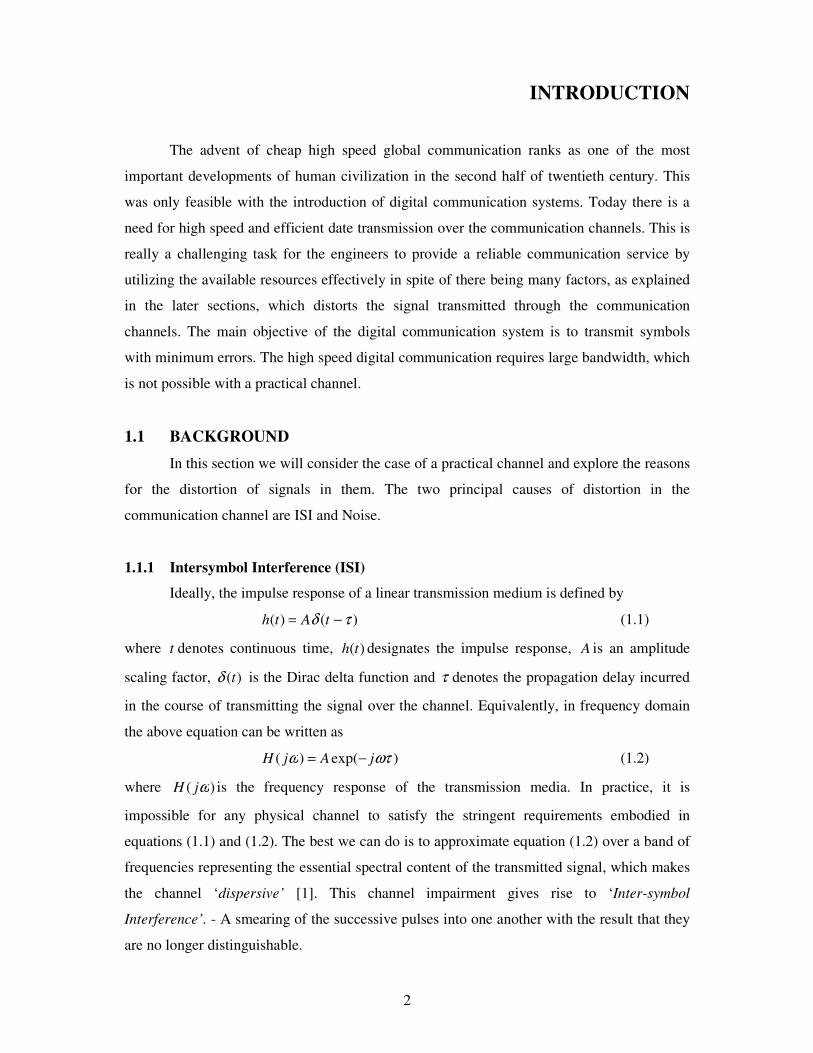
INTRODUCTION

The advent of cheap high speed global communication ranks as one of the most

important developments of human civilization in the second half of twentieth century. This

was only feasible with the introduction of digital communication systems. Today there is a

need for high speed and efficient date transmission over the communication channels. This is

really a challenging task for the engineers to provide a reliable communication service by

utilizing the available resources effectively in spite of there being many factors, as explained

in the later sections, which distorts the signal transmitted through the communication

channels. The main objective of the digital communication system is to transmit symbols

with minimum errors. The high speed digital communication requires large bandwidth, which

is not possible with a practical channel.

1.1 BACKGROUND

In this section we will consider the case of a practical channel and explore the reasons

for the distortion of signals in them. The two principal causes of distortion in the

communication channel are ISI and Noise.

1.1.1 Intersymbol Interference (ISI)

Ideally, the impulse response of a linear transmission medium is defined by

)()( τδ −= tAth (1.1)

where t denotes continuous time, )(th designates the impulse response, A is an amplitude

scaling factor, )(tδ is the Dirac delta function and τ denotes the propagation delay incurred

in the course of transmitting the signal over the channel. Equivalently, in frequency domain

the above equation can be written as

)exp()( ωτω jAjH −= (1.2)

where )( ωjH is the frequency response of the transmission media. In practice, it is

impossible for any physical channel to satisfy the stringent requirements embodied in

equations (1.1) and (1.2). The best we can do is to approximate equation (1.2) over a band of

frequencies representing the essential spectral content of the transmitted signal, which makes

the channel ‘dispersive’ [1]. This channel impairment gives rise to ‘Inter-symbol

Interference’. - A smearing of the successive pulses into one another with the result that they

are no longer distinguishable.

3

1.1.2 Noise

Some form of noise is always present at the output of every communication channel.

The noise can be internal to the system, as in case of thermal noise generated by the amplifier

at the front end of the receiver or external to the system, due to interfering signal originated

from other sources.

The net result of the two impairments is that the signal received at the channel output

is a noisy and distorted version of the signal that is transmitted. The function of the receiver is

to operate on the received signal and deliver a reliable estimate of the original message signal

to a user at the output of the system.

Hence there is a need for adaptive equalization. By equalization we mean the process

of correcting channel induced distortion. This process is said to be adaptive when it adjusts

itself continuously during data transmission by operating on the input [2]. The digital

communication scenario is illustrated in Fig.1.1.

Fig..11 Schematic of Digital communication system

In the figure )(ks is the transmitted data, the term )(kN represents the Additive White

Gaussian Noise (AWGN), )(kr is the received signal and )(ˆ dks − is an estimate of the

transmitted data. Here the term d is called the decision delay, the importance of which is

explained in chapter 3. Simply speaking the equalizer must perform the inverse operation of

the channel [3, 4]. The channel transfer function )(zH accounts for the ISI introduced by it.

1.1.3 Adaptive Equalization

It is very difficult for estimating both the channel order and the distribution of energy

among the taps and even it is very difficult to predict the effect of the environment on these

taps. Hence it is a must for the equalization process to be adaptive. The equalizer need to be

adapted very frequently with the changing environment. This includes two phases [5]. Firstly

the equalizer needs to be trained with some known samples in the presence of some desired

response (Supervised Learning). After training the weights and various parameters associated

4

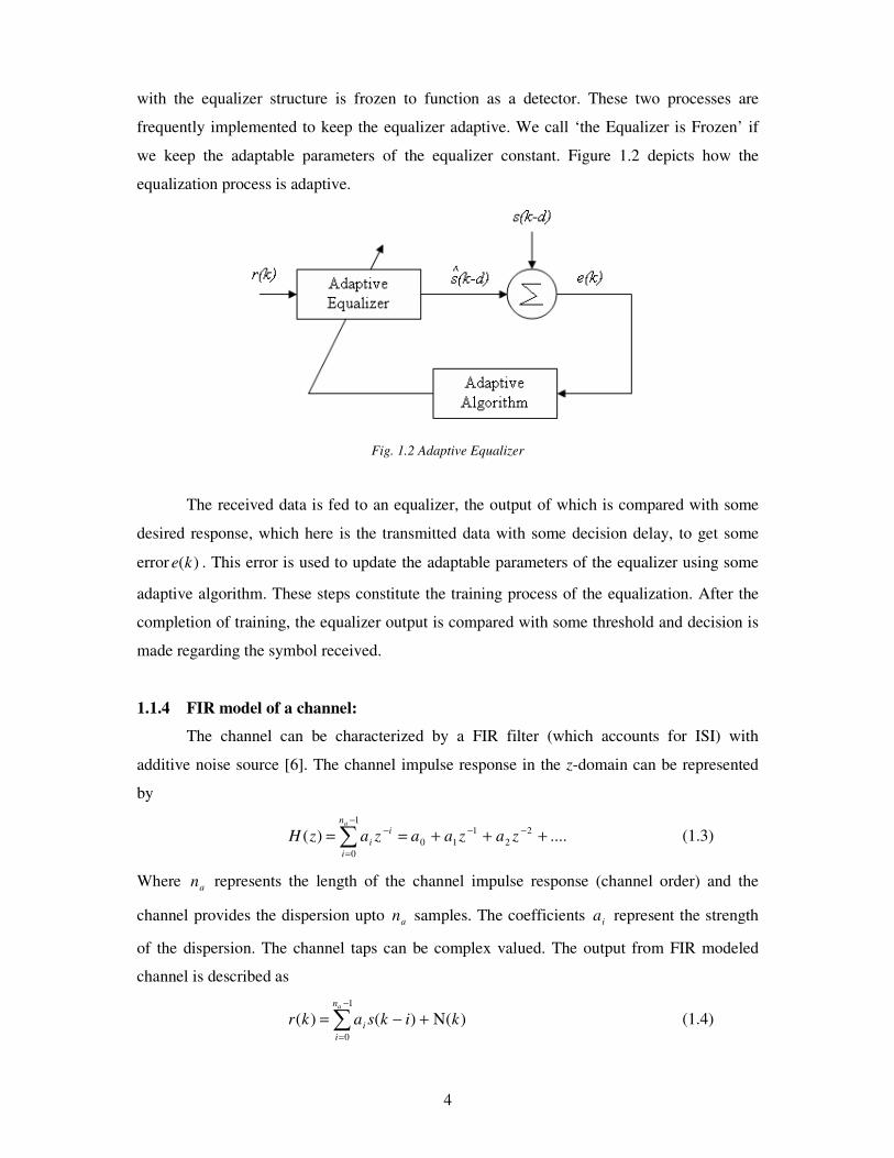
with the equalizer structure is frozen to function as a detector. These two processes are

frequently implemented to keep the equalizer adaptive. We call ‘the Equalizer is Frozen’ if

we keep the adaptable parameters of the equalizer constant. Figure 1.2 depicts how the

equalization process is adaptive.

Fig. 1.2 Adaptive Equalizer

The received data is fed to an equalizer, the output of which is compared with some

desired response, which here is the transmitted data with some decision delay, to get some

error )(ke . This error is used to update the adaptable parameters of the equalizer using some

adaptive algorithm. These steps constitute the training process of the equalization. After the

completion of training, the equalizer output is compared with some threshold and decision is

made regarding the symbol received.

1.1.4 FIR model of a channel:

The channel can be characterized by a FIR filter (which accounts for ISI) with

additive noise source [6]. The channel impulse response in the z-domain can be represented

by

....)( 2

2

1

10

1

0

+++==−−−

−

=

∑ zazaazazHi

n

i

i

a

(1.3)

Where a

n represents the length of the channel impulse response (channel order) and the

channel provides the dispersion upto a

n samples. The coefficients i

a represent the strength

of the dispersion. The channel taps can be complex valued. The output from FIR modeled

channel is described as

)()()(1

0

kiksakran

i

iΝ+−= ∑

−

=

(1.4)

5

Where )(kr is the observed channel output (which is input to the equalizer) and )(kΝ

represents (AWGN). For the case of computer simulations the taps of the FIR filter are

chosen at the signal’s sampling interval and coefficients chosen to accurately model the

impulse response.

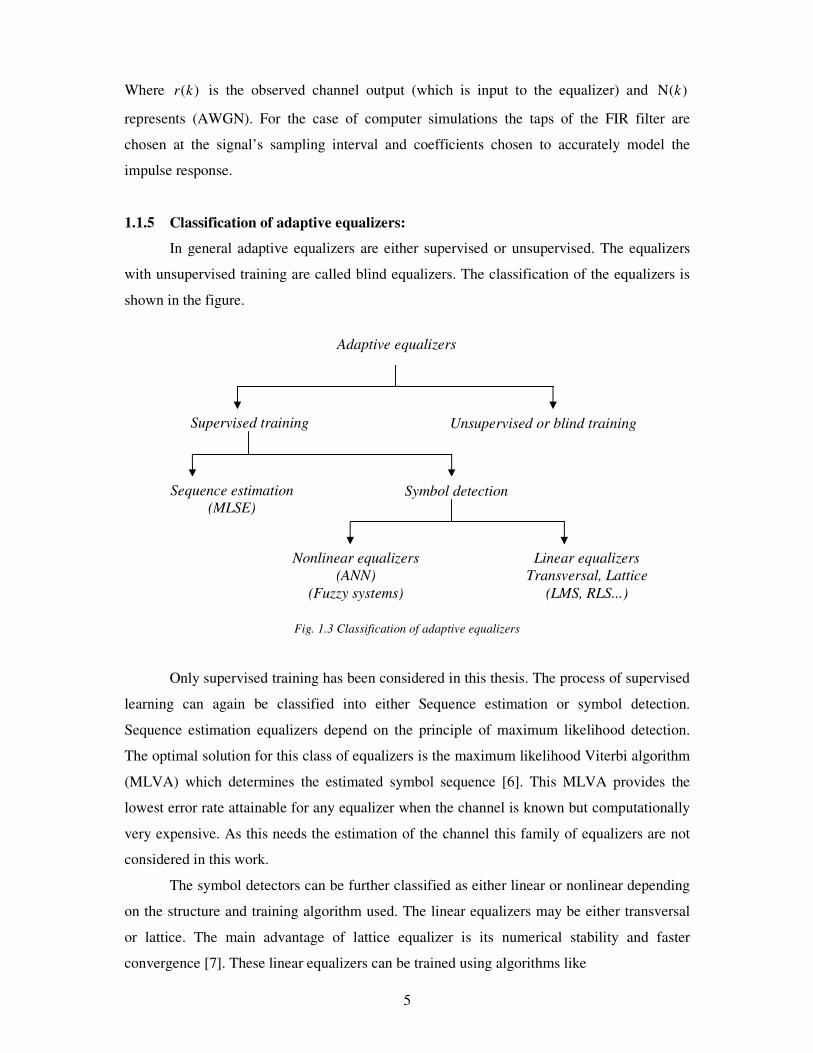
1.1.5 Classification of adaptive equalizers:

In general adaptive equalizers are either supervised or unsupervised. The equalizers

with unsupervised training are called blind equalizers. The classification of the equalizers is

shown in the figure.

Fig. 1.3 Classification of adaptive equalizers

Only supervised training has been considered in this thesis. The process of supervised

learning can again be classified into either Sequence estimation or symbol detection.

Sequence estimation equalizers depend on the principle of maximum likelihood detection.

The optimal solution for this class of equalizers is the maximum likelihood Viterbi algorithm

(MLVA) which determines the estimated symbol sequence [6]. This MLVA provides the

lowest error rate attainable for any equalizer when the channel is known but computationally

very expensive. As this needs the estimation of the channel this family of equalizers are not

considered in this work.

The symbol detectors can be further classified as either linear or nonlinear depending

on the structure and training algorithm used. The linear equalizers may be either transversal

or lattice. The main advantage of lattice equalizer is its numerical stability and faster

convergence [7]. These linear equalizers can be trained using algorithms like

Supervised training

Unsupervised or blind training

Sequence estimation

(MLSE)

Adaptive equalizers

Symbol detection

Nonlinear equalizers

(ANN)

(Fuzzy systems)

Linear equalizers

Transversal, Lattice

(LMS, RLS...)

6

(1) Zero Forcing Algorithm(ZF)

(2) Least Mean Square Algorithm(LMS)

(3) Recursive Least squares Algorithm(RLS)

The non-linear equalizers are used in applications where the channel distortion is too

severe for a linear equalizer to handle. There are few channels for which the decision

boundary is very complicated and a simple linear filter equalizer cannot perform well in those

cases. Further the process of equalization can be considered as the classification problem in

which the equalizer needs to classify the input vector into a number of transmitted symbols.

The optimal solution for the symbol detection equalizer is given by the Bayes Decision

theory [6, 8] which inherently is a nonlinear classifier. Hence structures which can

incorporate some amount of nonlinearity are required to obtain optimal or near optimal

solution. Some of the examples of nonlinear equalizers include those using Artificial Neural

Networks (ANNs), Fuzzy Systems etc. The thesis work mainly concentrates on the neural

network equalizers. The well known algorithm for training the neural network equalizer is the

Back Propagation (BP) Algorithm.

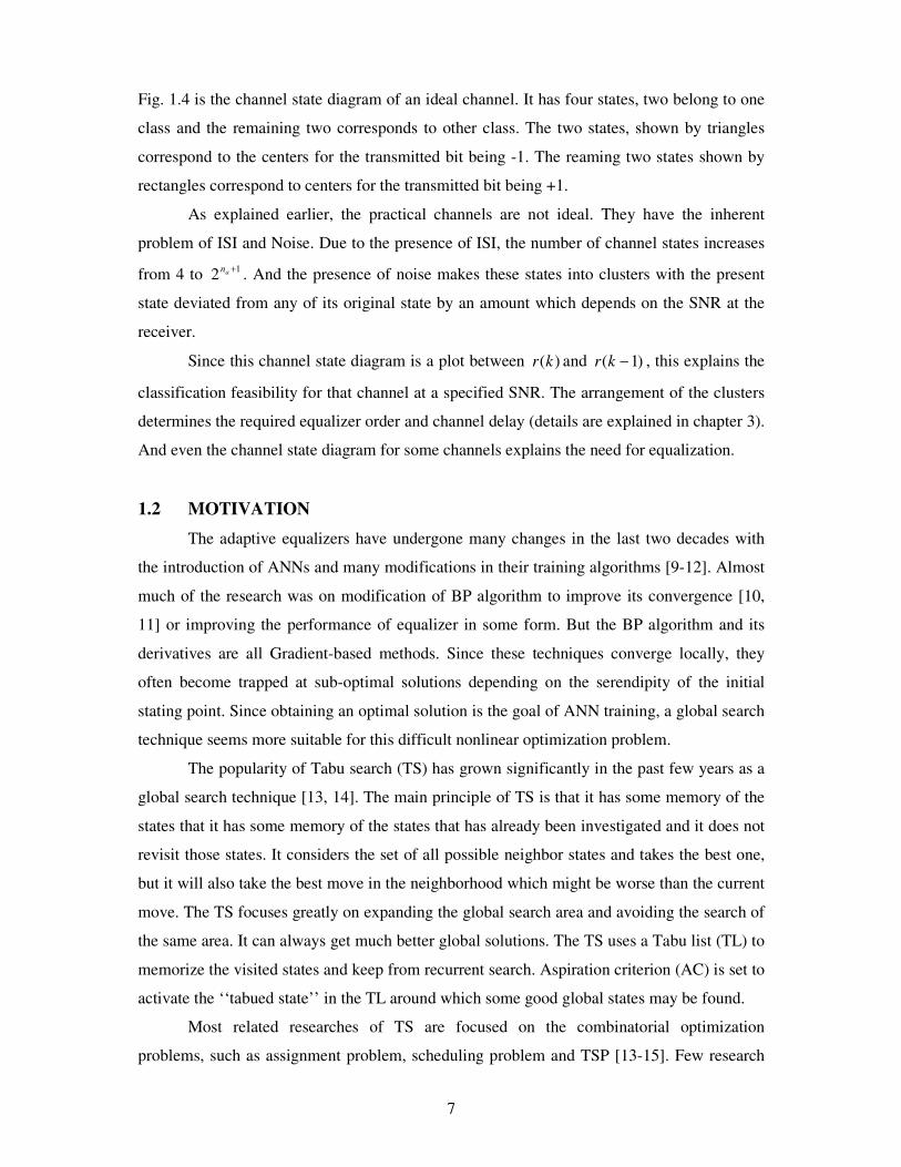
1.1.6 Channel State Diagram

A channel state diagram is a plot drawn between the present received sample )(kr ,on

x-axis and the previous sample )1( −kr , on y-axis.

-1.5

-1

-0.5

0

0.5

1

1.5

-2 -1.5 -1 -0.5 0 0.5 1 1.5 2

r(k)

r(k

-1)

Centers for symbol -1

Centers for symbol +1

Fig 1.4. Channel State Diagram for an Ideal Channel

7

Fig. 1.4 is the channel state diagram of an ideal channel. It has four states, two belong to one

class and the remaining two corresponds to other class. The two states, shown by triangles

correspond to the centers for the transmitted bit being -1. The reaming two states shown by

rectangles correspond to centers for the transmitted bit being +1.

As explained earlier, the practical channels are not ideal. They have the inherent

problem of ISI and Noise. Due to the presence of ISI, the number of channel states increases

from 4 to 1

2+an

. And the presence of noise makes these states into clusters with the present

state deviated from any of its original state by an amount which depends on the SNR at the

receiver.

Since this channel state diagram is a plot between )(kr and )1( −kr , this explains the

classification feasibility for that channel at a specified SNR. The arrangement of the clusters

determines the required equalizer order and channel delay (details are explained in chapter 3).

And even the channel state diagram for some channels explains the need for equalization.

1.2 MOTIVATION

The adaptive equalizers have undergone many changes in the last two decades with

the introduction of ANNs and many modifications in their training algorithms [9-12]. Almost

much of the research was on modification of BP algorithm to improve its convergence [10,

11] or improving the performance of equalizer in some form. But the BP algorithm and its

derivatives are all Gradient-based methods. Since these techniques converge locally, they

often become trapped at sub-optimal solutions depending on the serendipity of the initial

stating point. Since obtaining an optimal solution is the goal of ANN training, a global search

technique seems more suitable for this difficult nonlinear optimization problem.

The popularity of Tabu search (TS) has grown significantly in the past few years as a

global search technique [13, 14]. The main principle of TS is that it has some memory of the

states that it has some memory of the states that has already been investigated and it does not

revisit those states. It considers the set of all possible neighbor states and takes the best one,

but it will also take the best move in the neighborhood which might be worse than the current

move. The TS focuses greatly on expanding the global search area and avoiding the search of

the same area. It can always get much better global solutions. The TS uses a Tabu list (TL) to

memorize the visited states and keep from recurrent search. Aspiration criterion (AC) is set to

activate the ‘‘tabued state’’ in the TL around which some good global states may be found.

Most related researches of TS are focused on the combinatorial optimization

problems, such as assignment problem, scheduling problem and TSP [13-15]. Few research

8

works were done in the neural network learning. TS helps the NN learning process to the

gradient technique ‘‘jump out of’’ the local minima and get a great improvement on the

gradient technique. The TS can also be combined with other improved learning algorithms.

1.3 THESIS CONTRIBUTION

The main aim of the thesis is to develop novel neural network training algorithms that

overcome the problem of local minima and to reduce the structural complexity of the neural

network equalizer so that it can facilitate real time implementation with much ease.

Firstly a faster RLS based neural network training algorithm is developed. Here we

use the Recursive Least Squares (RLS) algorithm for updating the synaptic weights of the

neural network. It can be noted that using this algorithm convergence and hence training is

faster. But this RLS algorithm is also a Gradient based Algorithm [1]. Hence this algorithm

also has the problem of converging to local minima and hence no much improvement in

performance in terms of BER can be noted, with having the only advantage of reducing the

training time.

Secondly, the Tabu search (TS), which is famous as a global search algorithm, is used

in the training process of the equalizer. The work includes development of three neural

network learning algorithms, all based on TS. They can be summarized into two classes as

follows

(a) Tabu based BP algorithm: Here the synaptic weights of the neural network

are adapted using Tabu search (TS). This algorithm includes two phases -

Superficial Search (SS) and Deep Search (DS). BP algorithm is used in

both the SS and DS.

(b) Slope Adaptation using Tabu search: The slope of the activation function,

which is hyperbolic tangent in this case, is adapted using Tabu search. This

can again be done in two ways.

(i) First adapt the synaptic weights using BP algorithm and then

use TS for adapting the slope of the activation function.

(ii) In this case, both the weights and the slopes are adapted

parallely in each iteration. BP algorithm is used to adapt weight

and TS for adapting the slope.

Results show that the use of TS in both the cases, weight adaptation and slope adaptation,

improves the performance of the equalizer in terms of Bit Error Rate (BER) and also reduces

the structural complexity of the neural network.

9

1.4 THESIS LAYOUT

The transmitted symbols )(ks and the channel taps i

a can be complex valued. Here

they are restricted to real valued. This corresponds to the use of multilevel pulse amplitude

modulation (M-ary PAM) with a symbol constellation defined by

,12 −−= Misi

Mi ≤≤1 (1.5)

Concentration on the simpler real case allows us to highlight the basic principles and

concepts. Hence binary symbols )2( =M have been considered in the thesis as it provides a

very useful geometric visualization of equalization process. For the equalizer to classify, the

decision boundary must effectively partition the m-dimensional space into M-decision

regions.

In chapter 2, the use of neural networks as a nonlinear equalizer is explained. Here the

improvement in BER performance of the neural network equalizer over the linear equalizers

trained using LMS algorithm is shown. Also the need for nonlinear equalizers and decision

feedback is demonstrated in terms of the channel state diagrams. The decision feedback

equalizers (DFE) are explained.

Chapter 3 is dedicated to the discussion on various parameters influencing the

performance of the equalizer. The effect of changing these parameters is explained in this

chapter. Also, in this chapter, the importance of decision delay and its effect on BER

performance of the equalizer is considered.

In chapter 4 a new method of training the neural network using RLS is proposed. The

basic idea behind the RLS is explained and the proposed algorithm is given.

In chapter 5, the concept of Tabu search (TS) is explained and its application to neural

network is given. The algorithm for adapting the weights and slopes of the neural network is

presented. Chapter 6 is dedicated for results and discussion.

EQUALIZATION USING NEURAL NETWORKS

Introduction

Neural Network Equalizer

Decision Feedback Equalization

11

EQUALIZATION USING NEURAL NETWORKS

2.1 INTRODUCTION

Numerous advances have been made in developing intelligent systems, inspired by

biological neural networks. Researchers from many scientific disciplines are designing

artificial neural networks (ANNs) to solve a variety of problems in pattern recognition,

Function approximation, prediction, optimization, associative memory, and control.

Conventional approaches have been proposed for solving these problems. Although

successful applications can be found in certain well-constrained environments, none is

flexible enough to perform well outside its domain. ANNs provide exciting alternatives, and

many applications could benefit from using them.

2.2.1 Definition of Neural network

A neural network is a machine that is designed to model the way in which the brain

performs a particular task or function of interest. To achieve good performance, they employ

a massive interconnection of simple computing cells referred to as ‘Neurons’ or ‘processing

units’. Hence a neural network viewed as an adaptive machine can be defined as [16]

A neural network is a massively parallel distributed processor made up of simple

processing units, which has a natural propensity for storing experimental knowledge and

making it available for use. It resembles the brain in two respects:

1. Knowledge is acquired by the network from its environment through a

learning process.

2. Interneuron connection strengths, known as synaptic weights, are used to

store the acquired knowledge.

2.1.2 Importance

It is apparent that a neural network derives its computing power through, first, its

massively parallel distributed structure and, second, its ability to learn and therefore

generalize. The use of neural networks offers the following useful properties and capabilities:

o Massive parallelism

o Distributed representation and computation

o Learning ability

o Generalization ability

o Input-output mapping

12

o Adaptivity

o Uniformity of Analysis and Design

o Fault tolerance

o Inherent contextual information processing

o VLSI implentability.

The advent of neural networks marked the modeling of nonlinear adaptive systems

which could provide high degree of precision, fault tolerance and adaptability compared to

other forms of mathematical modeling [9]. So the artificial neural networks are

predominantly used for equalization. The Back Propagation (BP) algorithm is the best known

and widely used learning algorithm for training ANNs since its proposal by Rumelhart and

LeCun.

2.1.3 Need for nonlinear equalizers

The main reason nonlinear equalizers are preferred over their linear counterpart is that

the linear equalizers do not perform well on channels which have deep spectral nulls in the

passband. In an attempt to compensate for the distortion, the linear equalizer places too much

gain in the vicinity of the spectral nulls, thereby enhancing the noise present in these

frequencies.

Non-linear equalizers outperform the linear equalizers in terms of BER [17]. Also the

linear equalizers view equalization as inverse problem while non-linear equalizers view

equalization as a pattern classification problem.

Consider the following example of the channel states for the two channels.

1

1 5.01)( −

+= zzH and

21

2 3482.08704.03482.0)( −−

++= zzzH

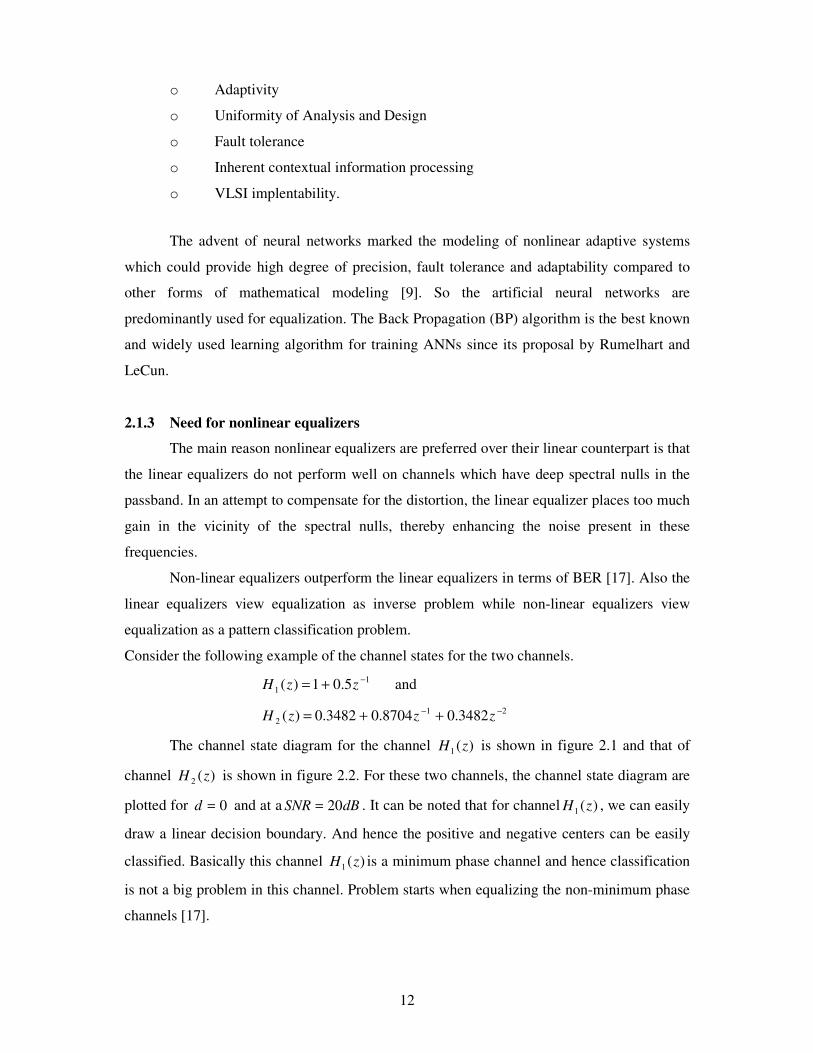
The channel state diagram for the channel )(1 zH is shown in figure 2.1 and that of

channel )(2 zH is shown in figure 2.2. For these two channels, the channel state diagram are

plotted for 0=d and at a dBSNR 20= . It can be noted that for channel )(1 zH , we can easily

draw a linear decision boundary. And hence the positive and negative centers can be easily

classified. Basically this channel )(1 zH is a minimum phase channel and hence classification

is not a big problem in this channel. Problem starts when equalizing the non-minimum phase

channels [17].

13

-2.5

-2

-1.5

-1

-0.5

0

0.5

1

1.5

2

2.5

-3.33 -2.33 -1.33 -0.33 0.67 1.67 2.67

r(k)

r(k-1

)

Centres For Symbol -1

Centres For Symbol +1

Fig. 2.1 Channel State diagram for )(1 zH

-2.5

-2

-1.5

-1

-0.5

0

0.5

1

1.5

2

2.5

-3.33 -2.33 -1.33 -0.33 0.67 1.67 2.67

r(k)

r(k-1

)

Centres For Symbol -1

Centres For Symbol +1

Fig. 2.2 Channel State diagram for )(2 zH

14

One of the popular channels belonging to this family is )(2 zH . It can be noted in

figure 2.2, for this channel, a simple linear decision boundary cannot classify the symbols

easily. It needs a nonlinear decision boundary or even a hyper-plane in multi-dimensional

channel space. Such a decision boundary cannot be achieved using a linear filter. Hence we

go for nonlinear structures which can adapt well to its environment are needed. Neural

networks serve this purpose.

2.2 NEURAL NETWORK EQUALIZER

These neural networks construct a functional relationship between input and output

patterns through the learning process, and memorize that relationship in the form of weights

for later applications [10]. The neural network equalizer outperforms the Linear Transversal

filters in terms of bit error rate (BER) as most of the communication channels requires

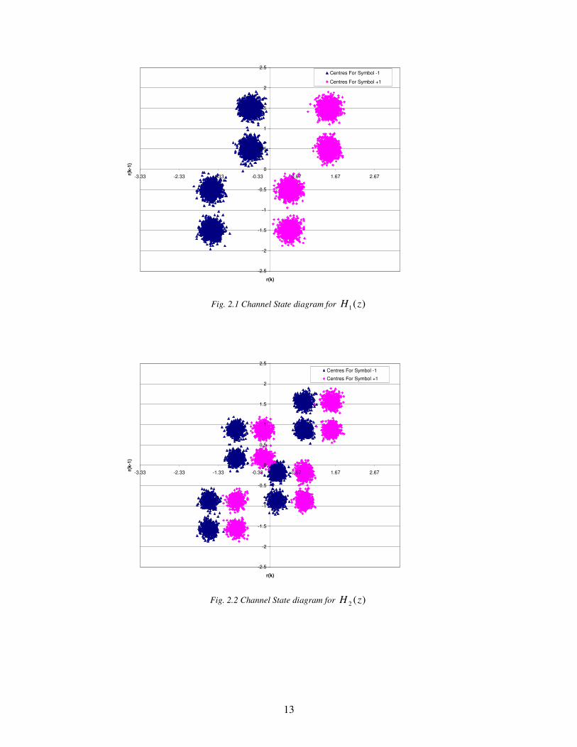
nonlinear decision boundary [17]. The structure of neural network equalizer is shown in the

figure.

In the figure )(kr represents received signal. The structure constitutes three significant

parts- one input layer, a set of hidden layers, one output layer. All the nodes are

interconnected by the weightsl

ijw , where i represents the destination node and j represents

the source node. The superscript l gives the layer number.

An equalizer of order m implies that it has m input nodes in its input layer as shown

in the figure. An equalizer will have a single node in its output layer. The signal received

sequentially is allowed to propagate through the hidden layers up to the node in the output

layer [9, 16].

Fig.2.3 Neural Network Equalizer

15

The output of the each node l

iy is the weighted sum of outputs of all the nodes in the

previous layer and affected by the activation function, which here is the hyperbolic tangent

function given by

ax

ax

e

ex

−

−

+

−

=

1

1)(φ (2.1)

where a represents the slope of the activation function.

Fig. 2.4 Hyperbolic Tangent Function with varying slopes

The figure 2.4 shows the hyperbolic tangent activation function with slope a varying

at 0.4, 0.8, 1.2 and 1.6. As slope increases the function tends towards threshold function. The

function attains a maximum value of +1 at ∞=x and a minimum value of -1 at −∞=x .

Hence the output of each node of the neural network will be in the range (-1, 1). Since we are

using binary PAM signal which takes either of the two values -1 or +1, this function is very

much suitable for equalization process.

Mathematically the forward propagation of the neural network is given by [16]

)(1

1

11

−

=

−

⋅=∑−

l

j

N

j

l

ij

l

iywv

l

(2.2)

l

iy = )( l

ivφ (2.3)

16

where l

iv is called the induced local field or activation potential of node i in layer l and

1−lN is the number of neurons in the layer )1( −l .

2.2.1 Back Propagation Algorithm

The BP algorithm is a very good example for the Gradient-based algorithms. The BP

algorithm consists of two passes through the different layers of the network: a forward pass

and a backward pass [16]. In the forward pass, as mentioned earlier, an activity pattern (input

vector) is applied to the sensory nodes of the network and its effect propagates through the

network layer by layer. Finally an output is obtained at the output node as the actual response

of the network. During the forward pass the synaptic weights are kept constant.

In the backward pass, on the other hand, the synaptic weights are all adjusted in

accordance with the error correction rule. The error signal, which is obtained by comparing

the output of the node in the output layer with the desired response, is allowed to pass against

the direction of synaptic weights (hence the name back propagation algorithm for this

training process) and local gradients l

iδ at each node is computed as given by Eqn.2.4.

)()(1

1

1 l

ji

N

i

l

i

l

j

l

jwv

l

⋅⋅′= ∑+

=

+

δφδ (2.4)

The local gradient )(nj

δ depends on whether neuron j is an input node or a hidden node:

(1) If neuron j is an output node, )(nj

δ equals the product of the derivative ))(( nvjj

ϕ ′

and the error signal )(nej

, both of which are associated with neuron j.

(2) If neuron j is a hidden node, )(nj

δ equals the product of the associated derivative

))(( nvjj

ϕ ′ and the weighted sum of the δ s computed for the neurons in the next

hidden or output layer that are connected to neuron j.

Due to the lack of availability of desired response at the hidden layers, it is not

possible to compute the error at these nodes. Hence this local gradient is very important in

providing the error measure at the hidden nodes. Using these local gradients the synaptic

weights update is given by Eqn. 2.5

•

•

=

∆+ l

i

l

j

l

jiy

ofneuron

linputsigna

gradient

local

parameter

telearningra

w

Correction

Weight

1δη

(2.5)

The weight correction l

jiw∆ is added to the present weight after each iteration. Once the

weights are updated till the mean square error (MSE) is below some desired threshold, the

17

weights are kept fixed. Now the designed equalizer is tested for its performance with 610

samples. This is called the testing phase of the equalizer. This testing is done by calculating

the bit error rate (BER) at different signal to noise ratio (SNR) values. This plot of SNR Vs

BER is the performance plot for an equalizer.

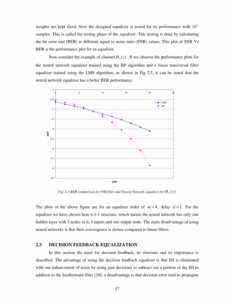
Now consider the example of channel )(2 zH . If we observe the performance plots for

the neural network equalizer trained using the BP algorithm and a linear transversal filter

equalizer trained using the LMS algorithm, as shown in Fig 2.5, it can be noted that the

neural network equalizer has a better BER performance.

-4.5

-4

-3.5

-3

-2.5

-2

-1.5

-1

-0.5

0

0 5 10 15 20 25

SNR

BE

R

LMS

BP

Fig. 2.5 BER comparison for FIR filter and Neural Network equalizer for )(2 zH

The plots in the above figure are for an equalizer order of 4=m , delay 1=d . For the

equalizer we have chosen here 4-3-1 structure, which means the neural network has only one

hidden layer with 3 nodes in it, 4 inputs and one output node. The main disadvantage of using

neural networks is that their convergence is slower compared to linear filters.

2.3 DECISION FEEDBACK EQUALIZATION

In this section the need for decision feedback, its structure and its importance is

described. The advantage of using the decision feedback equalizer is that ISI is eliminated

with out enhancement of noise by using past decisions to subtract out a portion of the ISI in

addition to the feedforward filter [18]; a disadvantage is that decision error tend to propagate

18

because they result in residual ISI and a reduced noise margin against noise at future

decisions.

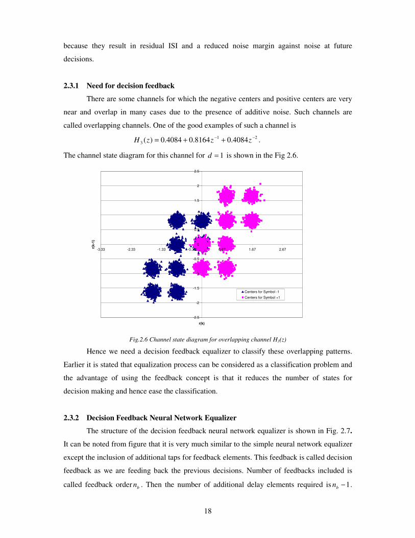
2.3.1 Need for decision feedback

There are some channels for which the negative centers and positive centers are very

near and overlap in many cases due to the presence of additive noise. Such channels are

called overlapping channels. One of the good examples of such a channel is

21

3 4084.08164.04084.0)( −−

++= zzzH .

The channel state diagram for this channel for 1=d is shown in the Fig 2.6.

-2.5

-2

-1.5

-1

-0.5

0

0.5

1

1.5

2

2.5

-3.33 -2.33 -1.33 -0.33 0.67 1.67 2.67

r(k)

r(k-1

)

Centers for Symbol -1

Centers for Symbol +1

Fig.2.6 Channel state diagram for overlapping channel H3(z)

Hence we need a decision feedback equalizer to classify these overlapping patterns.

Earlier it is stated that equalization process can be considered as a classification problem and

the advantage of using the feedback concept is that it reduces the number of states for

decision making and hence ease the classification.

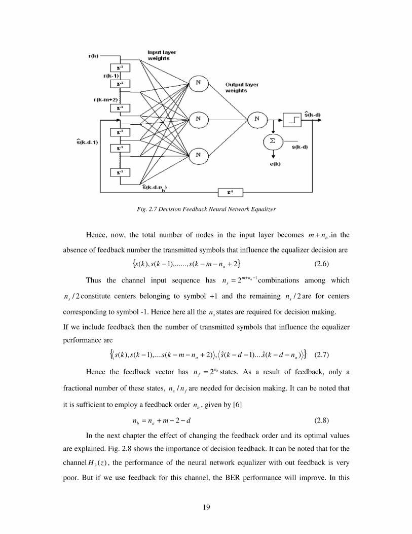
2.3.2 Decision Feedback Neural Network Equalizer

The structure of the decision feedback neural network equalizer is shown in Fig. 2.7.

It can be noted from figure that it is very much similar to the simple neural network equalizer

except the inclusion of additional taps for feedback elements. This feedback is called decision

feedback as we are feeding back the previous decisions. Number of feedbacks included is

called feedback orderb

n . Then the number of additional delay elements required is 1−b

n .

19

Fig. 2.7 Decision Feedback Neural Network Equalizer

Hence, now, the total number of nodes in the input layer becomes b

nm + .in the

absence of feedback number the transmitted symbols that influence the equalizer decision are

{ }2(),......,1(),( +−−−a

nmksksks (2.6)

Thus the channel input sequence has 1

2−+

=anm

sn combinations among which

2/s

n constitute centers belonging to symbol +1 and the remaining 2/s

n are for centers

corresponding to symbol -1. Hence here all the s

n states are required for decision making.

If we include feedback then the number of transmitted symbols that influence the equalizer

performance are

{ })(ˆ)....1(ˆ,)2(),....1(),(aa

ndksdksnmksksks −−−−+−−− (2.7)

Hence the feedback vector has bn

fn 2= states. As a result of feedback, only a

fractional number of these states, fs

nn / are needed for decision making. It can be noted that

it is sufficient to employ a feedback order b

n , given by [6]

dmnnab

−−+= 2 (2.8)

In the next chapter the effect of changing the feedback order and its optimal values

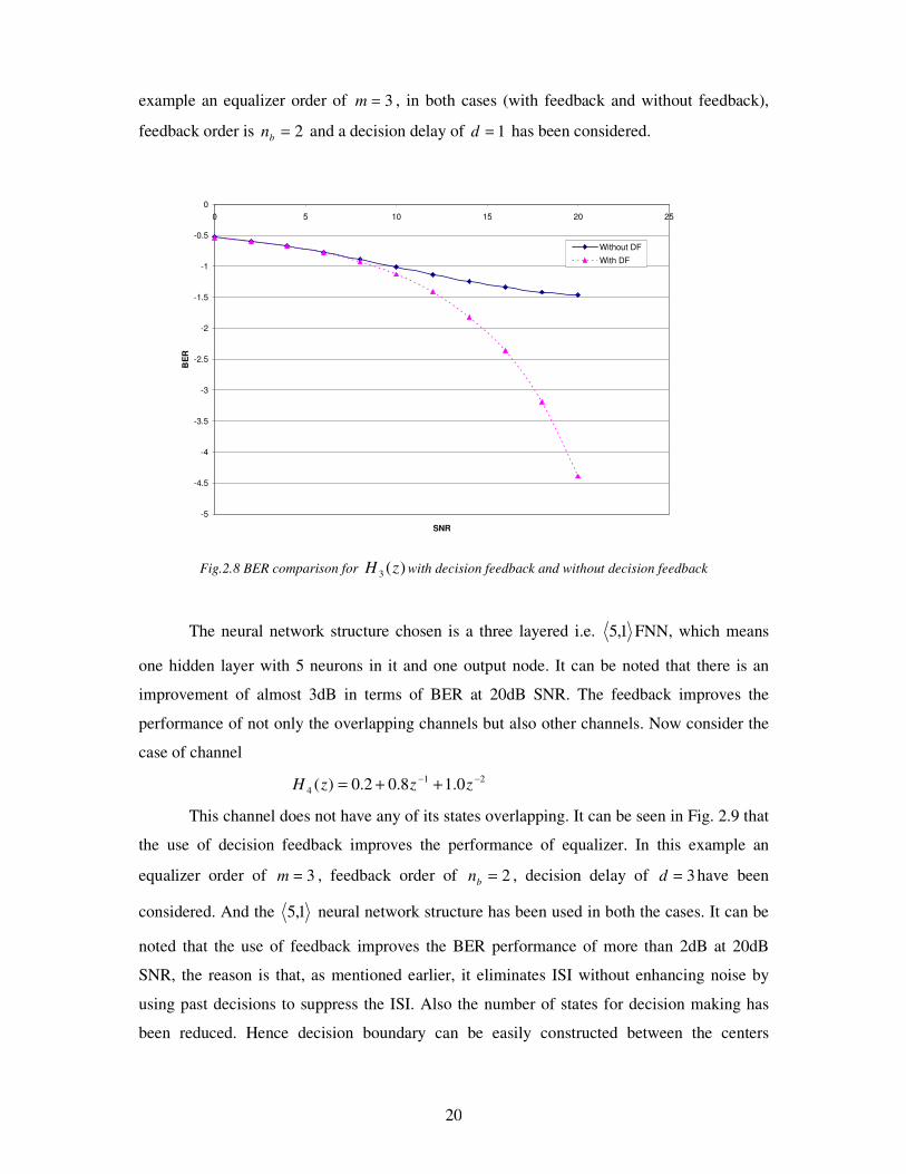
are explained. Fig. 2.8 shows the importance of decision feedback. It can be noted that for the

channel )(3 zH , the performance of the neural network equalizer with out feedback is very

poor. But if we use feedback for this channel, the BER performance will improve. In this

20

example an equalizer order of 3=m , in both cases (with feedback and without feedback),

feedback order is 2=b

n and a decision delay of 1=d has been considered.

-5

-4.5

-4

-3.5

-3

-2.5

-2

-1.5

-1

-0.5

0

0 5 10 15 20 25

SNR

BE

R

Without DF

With DF

Fig.2.8 BER comparison for )(3 zH with decision feedback and without decision feedback

The neural network structure chosen is a three layered i.e. 1,5 FNN, which means

one hidden layer with 5 neurons in it and one output node. It can be noted that there is an

improvement of almost 3dB in terms of BER at 20dB SNR. The feedback improves the

performance of not only the overlapping channels but also other channels. Now consider the

case of channel

21

4 0.18.02.0)( −−

++= zzzH

This channel does not have any of its states overlapping. It can be seen in Fig. 2.9 that

the use of decision feedback improves the performance of equalizer. In this example an

equalizer order of 3=m , feedback order of 2=b

n , decision delay of 3=d have been

considered. And the 1,5 neural network structure has been used in both the cases. It can be

noted that the use of feedback improves the BER performance of more than 2dB at 20dB

SNR, the reason is that, as mentioned earlier, it eliminates ISI without enhancing noise by

using past decisions to suppress the ISI. Also the number of states for decision making has

been reduced. Hence decision boundary can be easily constructed between the centers

21

belonging to symbol +1 and the centers belonging to symbol -1 and even the dimensionality

of the decision boundary can be reduced as there are lesser number of states.

-6

-5

-4

-3

-2

-1

0

0 5 10 15 20 25

SNR

BE

R

Without DF

With DF

Fig. 2.9. BER Comparison for )(4 zH with DF and without DF

Thus there is an additional advantage of using the decision feedback equalizers. They reduces

the equalizer order and hence the structural complexity of the equalizer.

PERFORMANCE OF EQUALIZER UNDER THE

INFLUENCE OF PARAMETER VARIATIONS

Effect of Additional noise level

Effect of Equalizer Order

Effect of Feedback Order

Effect of Decision Delay

23

PERFORMANCE OF EQUALIZER UNDER THE INFLUENCE

OF PARAMETER VARIATIONS

In this his chapter we will consider the influence of different parameters on equalizer

performance. In the symbol-by-symbol detection procedure for equalization we apply the

channel output which will be corrupted by both ISI and Noise, as described in the previous

chapter, to the equalizer which will classify the symbols into their respective classes. The

main goal of equalization is to minimize the misclassification rate.

It has been noted that the BER performance of the equalizer are influenced by many

factors which include the additional noise level, the equalizer order, the decision delay,

number of samples used for training, and the neural network structure we have considered. It

is noted in the earlier chapters that, for some channels classification is not possible without

feedback as they may have overlapping states and also seen that the BER performance of the

equalizer improves with the inclusion of feedback. Hence we get one more factor influencing

the classification capability of the equalizer.

So, we can say that the principal parameters that affect the equalizer’s BER performance are

(1) Additional noise level

(2) Equalizer order, m

(3) Feedback order, b

n

(4) Decision delay, d

In sections 3.1, 3.2, 3.3 and 3.4 we will compare the performance variations of the equalizers

with the change in any of these principal parameters. However, as mentioned, there are others

factors too, but their effect is not so appreciable. This will be discussed later in this chapter in

section 3.4 and 3.5.

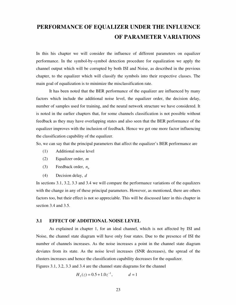
3.1 EFFECT OF ADDITIONAL NOISE LEVEL

As explained in chapter 1, for an ideal channel, which is not affected by ISI and

Noise, the channel state diagram will have only four states. Due to the presence of ISI the

number of channels increases. As the noise increases a point in the channel state diagram

deviates from its state. As the noise level increases (SNR decreases), the spread of the

clusters increases and hence the classification capability decreases for the equalizer.

Figures 3.1, 3.2, 3.3 and 3.4 are the channel state diagrams for the channel

,0.15.0)( 1

5

−

+= zzH 1=d

24

-5

-4

-3

-2

-1

0

1

2

3

4

5

-6.67 -4.67 -2.67 -0.67 1.33 3.33 5.33

r(k)

r(k-1

)

Centers For Symbol -1

Centers For Symbol +1

Fig. 3.1 Channel State Diagram for )(5 zH at SNR=5dB

-4

-3

-2

-1

0

1

2

3

4

-5.33 -3.33 -1.33 0.67 2.67 4.67

r(k)

r(k-1

)




25

-2.5

-2

-1.5

-1

-0.5

0

0.5

1

1.5

2

2.5

-3.33 -2.33 -1.33 -0.33 0.67 1.67 2.67

r(k)

r(k-1

)




-2.5

-2

-1.5

-1

-0.5

0

0.5

1

1.5

2

2.5

-3.33 -2.33 -1.33 -0.33 0.67 1.67 2.67

r(k)

r(k

-1)




26

Fig. 3.1 is plotted at an SNR=5dB. Here it can be noted that the point belonging to the cluster

of a positive centre and those of negative centers overlap to a large extent, hence

classification becomes difficult. Fig. 3.2, 3.3, 3.4 corresponds to the SNR values of 10dB,

15dB and 20dB respectively. As SNR increases, the problem of classification becomes easier.

3.2 EFFECT OF EQUALIZER ORDER

The effect of equalizer order is directly related to Covers Theorem [16]. This theorem

on the separability of patterns, which, in qualitative terms, may be stated as follows,

“A complex pattern-classification problem cast in a high-dimensional space

nonlinearly is more likely to be linearly separable than in a low-dimensional space.”

According to this theorem, as we move to higher dimensional space, classification becomes

easier. For an equalizer, increase in the equalizer order, m , increases the dimensionality of

the pattern space. And hence, an increase in the equalizer order eases the pattern

classification.

-6

-5

-4

-3

-2

-1

0

0 5 10 15 20 25

SNR

BE

R

m=2

m=3

m=4

m=5

m=6

Fig. 3.5 BER comparison for )(6 zH with varying m

Fig. 3.5 is the BER plot with varying equalizer order m . The plots are drawn for equalizers

of order 6,5,4,3,2=m , for the channel

321

6 3.00.13.02.0)( −−−

+++= zzzzH

27

For this channel, the plots are obtained with a 1,5 FNN structure and for decision delay

2=d . It can be seen from the plots that with an increase in equalizer order from 2 to 3, there

is an increase in equalizer performance of almost 1dB in terms of BER at the SNR value of

20dB. But if we increase the equalizer order further to 4, 5 or 6, there is no appreciable

change in performance. This is because for an equalizer, for a fixed value of decision

delay, d , an equalizer order of 1+= dm is sufficient [6]. And for the equalizer order of

1+> dm will almost have a similar performance and there will be no much appreciable

change in BER performance. Even in the example of )(6 zH , this phenomenon can be noted.

We have chosen an equalizer order of 2=d . And hence there will be no much improvement

in BER performance for 3>m compared to 3=m .

3.3 EFFECT OF FEEDBACK ORDER

As mentioned in the previous chapter, with the introduction of feedback, number of

states present while decision making decreases, hence classification becomes easier. Also as

feedback order increases, number of states decreases, hence performance increases as there is

an increase in margin existing between states. Fig. 3.6 shows the plots for varying feedback

order for the channel )(3 zH , with decision delay 1=d , equalizer order 2=m , and a neural

network structure 1,5 .

-4.5

-4

-3.5

-3

-2.5

-2

-1.5

-1

-0.5

0

0 2 4 6 8 10 12 14 16 18 20

SNR

BE

R

nb=0

nb=1

nb=2

Fig. 3.6 BER performance comparison for varying feedback order for )(3 zH

28

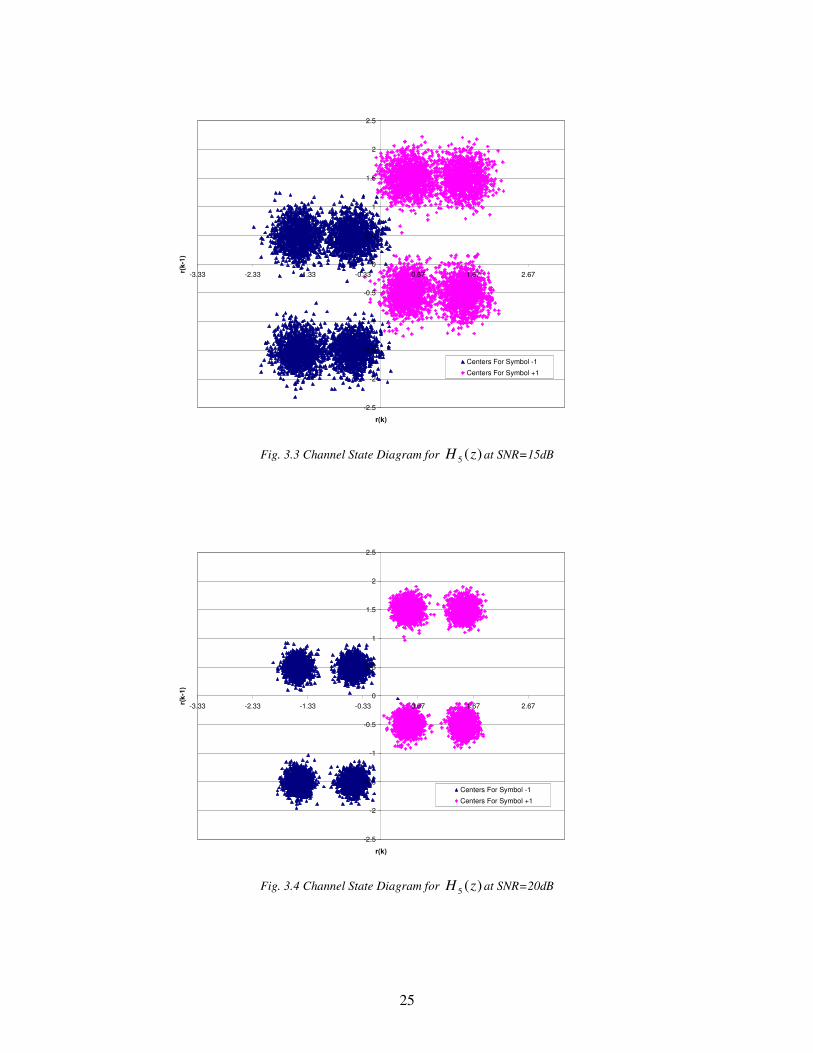
3.4 EFFECT OF DECISION DELAY

The effect of decision delay d , can be easily understood by observing its effect on the

channel state diagram.

-2.5

-2

-1.5

-1

-0.5

0

0.5

1

1.5

2

2.5

-3.33 -2.33 -1.33 -0.33 0.67 1.67 2.67

r(k)

r(k-1

)Centers For Symbol -1


Fig. 3.7 Channel state diagram for )(7 zH with 0=d and dBSNR 20=

-2.5

-2

-1.5

-1

-0.5

0

0.5

1

1.5

2

2.5

-3.33 -2.33 -1.33 -0.33 0.67 1.67 2.67

r(k)

r(k-1

)




29

-2.5

-2

-1.5

-1

-0.5

0

0.5

1

1.5

2

2.5

-3.33 -2.33 -1.33 -0.33 0.67 1.67 2.67

r(k)

r(k-1

)




-2.5

-2

-1.5

-1

-0.5

0

0.5

1

1.5

2

2.5

-3.33 -2.33 -1.33 -0.33 0.67 1.67 2.67

r(k)

r(k

-1)




The channel which has been considered for plotting the above figures 3.7-3.10, has a transfer

function given by

21

7 407.0815.0407.0)( −−

−−= zzzH

30

The channel state diagrams for the channel )(7 zH are drawn for the delay values of

3,2,1,0=d in Fig.3.7, 3.6, 3.9, 3.10 respectively. It can be noted from the above figures that

for the delay values of 2,1=d classification will be easier compared to those for delay

3,0=d . Hence certainly a superior performance is expected with the former delay values.

This can be seen in Fig. 3.11. there is a superior performance for delay values of 2,1=d .

-5

-4.5

-4

-3.5

-3

-2.5

-2

-1.5

-1

-0.5

0

0 5 10 15 20 25

SNR

BE

R

d=0

d=1

d=2

d=3

Fig. 3.11 BER performance comparison for varying decision delays for )(7 zH

Here a 1,5 FNN equalizer has been considered with out decision feedback with an equalizer

order 2=m .

However, the parameters b

ndm ,, are interdependent because, as explained earlier in

section 3.2, an equalizer order of 1+= dm is sufficient, any value more than this will not

give an appreciable increase in performance. From Eqn. 2.8,

dmnnab

−−+= 2 (3.1)

Hence substituting 1+= dm in above equation we get,

1−=ab

nn (3.2)

I.e. a proper combination of these parameters, for a chosen channel order, is required to

obtain a better performance (near optimal) of the equalizer.

RLS BASED BP ALGORITHM

Introduction to RLS

Neural Network Training using RLS

32

RLS BASED BP ALGORITHM

In this chapter, the novel method of training the neural network using RLS algorithm is

introduced. In section 4.1, a brief introduction to the RLS algorithm is given and in section

4.2 the proposed method of training neural networks using RLS is explained and the

corresponding algorithm is given.

4.1 INTRODUCTION TO RLS

RLS algorithm was actually introduced to improve the rate of convergence of the

linear adaptive filters. This RLS algorithm is an extension to the method of least squares [1].

This algorithm was developed on the basis of a relation in matrix algebra known as “Matrix

Inversion Lemma”. An important feature of this algorithm is that its rate of convergence is

typically an order of magnitude faster than the simple LMS filter, due to the fact that the RLS

filter whitens input data by using the inverse correlation matrix of the data, assumed to be of

zero mean.

The recursive implementations of the method of least squares starts with prescribed

initial conditions and use the information contained in new data samples to update the old

estimates. Hence here the length of the observable data is variable. Accordingly, the cost

function [1, 4] to be minimized can be expressed as

∑=

−

=

k

i

ikiek

1

2)()( λξ (4.1)

where k is the variable length of the observable data, λ is a positive constant close to but less

than unity and is called the “Forgetting Factor”. The use of this forgetting factor is intended

to ensure that data in the distant past are “forgotten” in order to afford the possibility of the

statistical variations of the observable data when the filter operates in a non-stationary

environment. The special case of 1=λ corresponds to the ordinary method of least squares.

4.1.1 Regularization

Least-squares estimation, like the method of least-squares, is an ill-posed inverse

problem, in that the input data consisting of tap-input vector )(ky and the corresponding

desired response )(kd for varying k are given, and the requirement is to estimate the

unknown parameter vector of a multiple regression model that relates )(kd to )(ky .

The ill-posed nature of least squares estimation is due to the following reasons:

33

• There is insufficient information in the input data to reconstruct the input-output

mapping uniquely.

• The unavoidable presence of noise or imprecision in the input data adds uncertainty to

the reconstructed input-output mapping.

To make the estimation problem “well posed”, some form of prior information about

the input-output mapping is needed. This, in turn, means that the formulation of the cost

function must be expanded to take the prior information into account. To satisfy this

objective, the cost function to be minimized can be written as,

2

1

2)()()( kiek

k

k

i

ikwθλλξ +=∑

=

− (4.2)

The second term in the summation is called the regularization term and θ is a positive real

number called the “Regularization Parameter”. Except for the factor kθλ , the regularization

term depends on the tap weight vector )(nw .

Hence the MM × time-average correlation matrix of the input vector )(iy can be given by

Ι+=Φ ∑=

− k

k

i

Hikiik θλλ

1

)()()( yy (4.3)

In the above equation, Ι is the MM × identity matrix. It can be noted that the addition of the

regularization term has the effect of making the correlation matrix )(kΦ nonsingular at all

stages of the computation, starting from 0=k .The weight update in the RLS algorithm is

given by

)()()1(ˆ)(ˆ kkkk∗

+−= ξgww (4.4)

Where )(kg is called the gain vector, which is given by

)()()( 1kkk yg −

Φ= (4.5)

Hence the weight update requires the calculation of the inverse of the correlation matrix

)(kΦ .

4.1.2 The Matrix Inversion Lemma

Let A and B be two positive-definite MM × matrices related by

HCCDBA 11 −−

+= (4.4)

Where D is a positive-definite MN × matrix and C is an NM × matrix. According to the

matrix inversion lemma, the inverse of the matrix A can be expressed as

BCBCCDBCBA HH 11 )( −−

+−= (4.5)

34

The main advantage of using this concept is that, it helps update weights with out actually

determining the inverse of the correlation matrix. It instead updates the gain vector itself.

Here we first declare some matrix P as the inverse of the correlation matrix. We initialize it

with some small values and then update it in each iteration. Using this updated inverse

correlation matrix we determine the gain vector )(kg in each iteration and use it in updating

the weights.

4.1.3 Importance of RLS

a. In the LMS algorithm, the correction that is applied in updating the old estimate of the

coefficient vector is based on the instantaneous sample value of the tap-input vector

and the error signal. On the other hand, in the RLS algorithm the computation of this

correction utilizes all the past available information.

b. In the LMS algorithms, the correction applied to the previous estimate consists of the

product of three factors: the (scalar) step-size parameterη , the error signal )1( −ke ,

and the tap-input vector u(n-1). On the other hand, in the RLS algorithm this

correction consists of the product of two factors: the true estimation error )1( −kξ and

the gain vector )(kg . The gain vector itself consists of )(1

k−

Φ , the inverse of the

deterministic correlation matrix, multiplied by the tap-input vector )(ky . The major

difference between the LMS and RLS algorithms is therefore the presence of )(1k

−

Φ

in the correction term of the RLS algorithm that has the effect of de-correlating the

successive tap inputs, thereby making the RLS algorithm self-orthogonalizing.

Because of this property, we find that the RLS algorithm is essentially independent of

the eigen value spread of the correlation matrix of the filter input.

c. The LMS algorithm requires approximately 20M iterations to converge in mean

square, where M is the number of tap coefficients contained in the tapped-delay-line

filter. On the other band, the RLS algorithm converges in mean square within less

than 2M iterations. The rate of convergence of the RLS algorithm is therefore, in

general, faster than that of the LMS algorithm by an order of magnitude.

d. Unlike the LMS algorithm, there are no approximations made in the derivation of the

RLS algorithm. Accordingly, as the number of iterations approaches infinity, the

least-squares estimate of the coefficient vector approaches the optimum Wiener value,

and correspondingly, the mean-square error approaches the minimum value possible.

35

In other words, the RLS algorithm, in theory, exhibits zero mis-adjustment. On the

other hand, the LMS algorithm always exhibits a nonzero mis-adjustment; however,

this mis-adjustment may be made arbitrarily small by using a sufficiently small step-

size parameter η .

4.2 NEURAL NETWORK TRAINING USING RLS

The method of training the neural network using the RLS algorithm is explained in

this section. The RLS algorithm is used to update the synaptic weights of the neural

networks. The proposed algorithm is almost similar to the Back Propagation (BP) algorithm

except the step of weight update changes. This algorithm also has two passes, a forward pass

and a backward pass. In the forward ass, the inputs are allowed to propagate through the

network, till it reaches the output node. Then, at the output node, error is calculated and back

propagated through the network. During the back propagation of error, the local gradient, l

jδ ,

is computed at each node. The subscripts and superscripts used are already explained in

chapter 2.

For using RLS to update the weights of the neural networks, each node in all the

layers of the neural network should maintain a window of their past outputs. Also separate

inverse correlation matrices and gain vectors need to be maintained at each node (including

the input node and excluding the output node). The size of the window and the size of these

matrices depend on the number of nodes in the next layer. Here the simple RLS algorithm is

applied at each node.

4.2.1 Algorithm

The algorithm for the proposed method of training the neural network using the RLS

algorithm is presented below:

a. Initialize the algorithm by setting small random values to all the synaptic weights.

b. Initialize the inverse correlation matrix )0(l

iP at each node.

IP ⋅=−1)0( θ

l

i (4.6)

where i represents the thi node in layer l , this matrix is of the order

11 ++×

llNN

and 1+lN represents number of nodes in layer )1( +l , and θ is a small constant.

c. Initialize 1=n and continue steps d-j for maximum number of iterations.

d. Forward propagation of the inputs, which is same as in BP algorithm.

36

e. Compute the error e at the output.

f. Back propagate the error to calculate the local gradient )(nl

iδ at each node which is

same as in BP algorithm.

g. Compute an intermediate matrix )(nl

iπ .

)()1()( nnnl

i

l

i

l

iYP ⋅−=π (4.7)

Where )(nl

iY represents the windowed output at each node, the order of this

matrix being 11 ×+l

N .

h. Compute the gain vector )(nl

iK , whose size is 11 ×

+lN .

))()((

)()(

nn

nn

l

i

Tl

i

l

il

i

πλ

π

⋅+

=

YK (4.8)

Where the constant λ is called the forgetting factor, the superscript T represents

the transpose of the matrix.

i. Update the weights.

)()()1()( 1nnKnwnw

l

j

l

ji

l

ji

l

ji

+

⋅+−= δ (4.9)

Where )(nKl

jiis a scalar and gives the th

j value of the gain vector )(nl

iK

j. Update the inverse correlation matrix.

)1()()()1()( 11−⋅⋅⋅−−⋅=

−−

nnnnnl

i

Tl

i

l

i

l

i

l

iPYKPP λλ (4.10)

RESULTS AND DISCUSSION

RLS based BP algorithm

48

RESULTS AND DISCUSSION

In this chapter, the results obtained using the proposed algorithms of using RLS and TS for

training the neural network are shown and the improvement in performance either in terms of

convergence or bit error rate are discussed. In section 6.1 the results using the RLS algorithm

for training ANNs are presented. In section 6.2, the behavior of the tabu based weight

updating is discussed and in the last section, 6.3, the advantage of using the TS for slope

adaptation is explained. All the programs are written in C and compiled using Microsoft

VC++ ver.6.0 and the plots are taken using Microsoft Excel-2003.

6.1 RLS BASED BP ALGORITHM

In this experiment, it is shown that when RLS algorithm is used to update the weights

of a neural network, the rate of convergence is faster compared to training using simple BP

algorithm. The channel, considered is having the transfer function

321

6 3.00.13.02.0)( −−−

+++= zzzzH

Here, the neural network structure used is 1,5 FNN with an equalizer order,

4=m and the decision delay 3=d . No feedback is employed in this experiment. The

convergence plots, which is the plot of mean square error against the iteration number, for the

channel is shown in Fig. 6.1 for the two cases of RLS based training and BP algorithm. The

plots are taken for 1000 iterations. It can be noted from these convergence plots that the

proposed algorithm provides a rate of convergence faster than the simple BP algorithm.

Hence the use of this algorithm reduces the training time and hence very much suitable for

high speed digital communication systems.

When a neural network is trained for smaller number of iteration, then the RLS based

training will have a superior performance, in terms of BER, compared to the case of training

using BP algorithm. This is shown in Fig. 6.2, where the neural network is trained for 150

iterations and tested using 610 samples. From the figure it can be noted that there is an

improvement of over 1.5dB in terms of BER at 20dB SNR.

But when we train the neural network for more number of iteration then there may not

be much improvement in performance. The reason being that both the BP algorithm and the

RLS based neural network training algorithms are derived from the Gradient-based learning

algorithms. Hence it too have the problem of getting trapped in the local minima. Fig. 6.3

shows that the BP algorithm needs more iterations to achieve the same performance.

49

-0.2

0

0.2

0.4

0.6

0.8

1

1.2

0 200 400 600 800 1000 1200

Iterations

MS

EMLP-BP

MLP-RLS

Fig. 6.1 Convergence plots for BP and RLS algorithms

-4.5

-4

-3.5

-3

-2.5

-2

-1.5

-1

-0.5

0

0 5 10 15 20 25

SNR

BE

R

MLP-BP

MLP-RLS

Fig. 6.2 SNR Vs BER plots for RLS and BP when trained for 150 iterations

50

-5

-4.5

-4

-3.5

-3

-2.5

-2

-1.5

-1

-0.5

0

0 5 10 15 20 25

SNR

BE

R

MLP-BP

MLP-RLS

Fig. 6.3 SNR Vs BER for BP trained for 2000 iterations and RLS trained for 200 iterations

CONCLUSION

58

CONCLUSIONS

In this dissertation, the importance of artificial neural networks as nonlinear adaptive

equalizers has been studied. The influence of different parameters on equalizers performance

is observed. Various algorithms for training the neural network are presented. Among them

the first one is the use of Recursive Least Square (RLS) algorithm for updating the weights of

the neural network to improve the rate of convergence. It is noted that the use of this

algorithm accelerates the training process and even provide better performance in terms of

Bit Error Rate (BER), when trained for smaller number of iterations. But if they are trained

with more number of iterations, there may not be appreciable increase in performance

compared to that of training using BP algorithm, as both of them belong to the family of

Gradient-based training algorithms, which are more likely to stop at some local minima.

Results show that the two proposed algorithms give superior performance. But

among applications. It is also shown that the proposed algorithms not only improves the

equalizer performance but also reduces the structural complexity of the neural network.

Any other superior optimization algorithms like Particle Swarm Optimization (PSO)

may be used to adapt the weights. The use of these algorithms may give a superior result.

59

REFERENCES

[1] Haykin. S. Adaptive Filter Theory. Delhi: 4th

Ed, Pearson Education, 2002

[2] Haykin. S. Digital Communication. Singapore: John Wiley & Sons Inc,1988.

[3] Proakis. J. G. Digital Communications. New York: McGraw-Hill, 1983.

[4] Qureshi. S. U. H, “Adaptive equalization,” Proc. IEEE, vol. 73, no.9, pp.1349-

1387, 1985.

[5] Widrow. B and Stearns. S. D. Adaptive Signal Processing. Englewood Cliffs, NJ:

Prentice Hall, 1985.

[6] Chen. S, Mulgrew. B and Mclaughlin. S, “Adaptive Bayesian equalizer with

decision feedback”, IEEE Trans. Signal Processing, Vol. 41, No. 9, Sept 1993

[7] T. S. Rapport. Wireless Communications. Delhi: Pearson Education, 2000.

[8] Duda. R. O and Hart. P. E. Pattern Classification and Scene Analysis. New York:

John Wiley & Sons Inc, 1973.

[9] Lippmann. R. P, “An Introduction to Computing with Neural Nets”, IEEE ASSP

Magazine, pp.4-22, April 1987.

[10] Kim. M. C and Choi. C. H, "Square root learning in batch mode BP for

classification problems," Proc. of ICNN, pp. 2769-2774, Nov. 1995.

[11] Zainuddin. Z, Mahat. N, Abu Hassan. Y, “Improving the Convergence of the

Backpropagation Algorithm Using Local Adaptive Techniques”, Proc. of ICCI,

pp.173-176, Dec. 2004.

[12] Zhang. De-Xian, Liu. Can, Wang. Zi-Quiang, Liu. Nan-Bo, “A New Fast

Learning Algorithm for Multilayer Feed Forward Neural Network”, IEEE Proc. of

ICMLC, (August 2006): pp- 2928-2934.

[15] Hertz A, Taillard E, de Werra D. “A Tutorial on Tabu Search”. Proc. of Giornate

di Lavoro AIRO'95 (Enterprise Systems: Management of Technological and

Organizational Changes), (1995), pp13-24.

[16] Haykin. S. Neural Networks: A Comprehensive Foundation. Delhi: 2nd

Ed,

Pearson Education, 2001

[17] Gibson. G. J, Siu. S, Cowan. C. F. N, “Multilayer Perceptron Structures Applied

to Adaptive Equalizers for Data Communications”, International Conference on

Acoustics, Speech and Signal Processing, vol. 2, pp.1183-1186, May 1989.

60

[18] Siu. S, Gibson. G. J and Cowan. C. F.N, “Decision feedback equalization using

neural network structures and performance comparison with standard

architecture”, IEE Proceedings part I, vol. 137, no. 4, pp. 221-225, Aug 1990.

designing an equalizer structure using gradient descent...

Documents