Detectability of CO2 flux signals by a space-basedlidar missionDorit M. Hammerling1,2, S. Randolph Kawa3, Kevin Schaefer4, Scott Doney5, and Anna M. Michalak6

1Department of Civil and Environmental Engineering, University of Michigan, Ann Arbor, Michigan, USA, 2Now at Institutefor Mathematics Applied to Geosciences, National Center for Atmospheric Research, Boulder, Colorado, USA, 3NASAGoddard Space Flight Center, Greenbelt, Maryland, USA, 4National Snow and Ice Data Center, Cooperative Institute forResearch in Environmental Sciences, University of Colorado at Boulder, Boulder, Colorado, USA, 5Department of MarineChemistry and Geochemistry, Woods Hole Oceanographic Institution, Woods Hole, Massachusetts, USA, 6Department ofGlobal Ecology, Carnegie Institution for Science, Stanford, California, USA

Abstract Satellite observations of carbon dioxide (CO2) offer novel and distinctive opportunities forimproving our quantitative understanding of the carbon cycle. Prospective observations include thosefrom space-based lidar such as the active sensing of CO2 emissions over nights, days, and seasons (ASCENDS)mission. Here we explore the ability of such a mission to detect regional changes in CO2 fluxes. We investigatethese using three prototypical case studies, namely, the thawing of permafrost in the northern high latitudes,the shifting of fossil fuel emissions from Europe to China, and changes in the source/sink characteristics ofthe Southern Ocean. These three scenarios were used to design signal detection studies to investigate theability to detect the unfolding of these scenarios compared to a baseline scenario. Results indicate that theASCENDS mission could detect the types of signals investigated in this study, with the caveat that the studyis based on some simplifying assumptions. The permafrost thawing flux perturbation is readily detectableat a high level of significance. The fossil fuel emission detectability is directly related to the strength of thesignal and the level of measurement noise. For a nominal (lower) fossil fuel emission signal, only the idealizednoise-free instrument test case produces a clearly detectable signal, while experiments with more realisticnoise levels capture the signal only in the higher (exaggerated) signal case. For the Southern Ocean scenario,differences due to the natural variability in the El Niño–Southern Oscillation climatic mode are primarilydetectable as a zonal increase.

1. Introduction

Satellite observations of carbon dioxide (CO2) offer novel and distinctive opportunities for improving ourquantitative understanding of the carbon cycle, which is an important scientific and societal challenge withanthropogenic CO2 emissions still on the rise. Prospective new observations include those from space-basedlidar such as the active sensing of CO2 emissions over nights, days, and seasons (ASCENDS) mission, whichis proposed in “Earth Science and Applications from Space: National Imperatives for the Next Decade”[National Research Council, 2007] (henceforth referred to as the decadal survey). Notable features of thismission include its ability to sample at night and at high latitudes. These conditions are prohibitive to passivemissions, such as the Greenhouse gases Observing SATellite [e.g., Kuze et al., 2009; Yokota et al., 2009] and theOrbiting Carbon Observatory-2 missions [e.g., Crisp et al., 2004], due to their reliance on reflected sunlight.The lidar measurement technique proposed for the ASCENDS mission further enables observing throughsome clouds and aerosols [Ehret et al., 2008], which also represent impediments and potential sources ofbias for passive missions [e.g.,Mao and Kawa, 2004]. Extensive instrument design research and developmentare ongoing, and proof of concept and validation studies indicate that ASCENDS will be able to providehigh-precision, unbiased observations with improved spatial coverage compared to passive missions[e.g., Spiers et al., 2011; Abshire et al., 2010; Kawa et al., 2010].

The primary goals of the ASCENDS mission are to address open questions in carbon cycle science that focuson the identification of changing source/sink characteristics that are difficult to observe using other currentor anticipated observations. These goals were first articulated in the decadal survey [National ResearchCouncil, 2007] and later refined in an ASCENDS mission NASA Science Definition and Planning Workshop[Active sensing of CO2 emissions over nights, days, and seasons (ASCENDS) Workshop Steering Committee, 2008].

HAMMERLING ET AL. ©2015. American Geophysical Union. All Rights Reserved. 1794

PUBLICATIONSJournal of Geophysical Research: Atmospheres

RESEARCH ARTICLE10.1002/2014JD022483

Key Points:• Detectability of regional changes inCO2 fluxes by space-based lidar

• Permafrost thawing flux perturbationreadily detectable by ASCENDS-likemission

• Southern Ocean ENSO-related fluxvariability detectable as zonal change

Supporting Information:• Figures S1–S8

Correspondence to:D. M. Hammerling,dorith@ucar.edu

Citation:Hammerling, D. M., S. R. Kawa, K. Schaefer,S. Doney, and A. M. Michalak (2015),Detectability of CO2 flux signals by aspace-based lidarmission, J. Geophys. Res.Atmos., 120, 1794–1807, doi:10.1002/2014JD022483.

Received 25 AUG 2014Accepted 5 JAN 2015Accepted article online 8 JAN 2015Published online 11 MAR 2015

They include detecting changes in the northern high-latitude sources and sinks, detecting changes inSouthern Ocean source/sink characteristics, constraining anthropogenic CO2 emissions, and increasing ourunderstanding of biospheric carbon dynamics by differentiating photosynthetic and respiration fluxes[ASCENDS Workshop Steering Committee, 2008]. CO2 fluxes in the northern high latitudes and in the SouthernOcean may change substantially as climate evolves, for example, and it is crucial to detect and attribute suchchanges quickly as they could lead to large increases in atmospheric CO2 concentrations and subsequentshifts in climate dynamics [e.g., Canadell et al., 2010].

Guided by these stated goals, this study explores the extent to which a space-based lidar mission, using theASCENDS mission concept as a guideline, can indeed contribute to these pertinent carbon cycle sciencequestions. We specifically focus on the ability of such amission to detect regional changes in fossil fuel emissions,high-latitude CO2 fluxes, and CO2 fluxes in the Southern Ocean. We investigate these using three prototypicalcase studies, namely, the thawing of permafrost in the northern high latitudes, the shifting of fossil fuel emissionsfrom Europe to China, and changes in the source/sink characteristics of the Southern Ocean related to theEl Niño–Southern Oscillation (ENSO). Realistic flux scenarios are defined for each of these prototypical casestudies within the anticipated time frame of the ASCENDS mission (i.e., the early to mid-2020s). These fluxscenarios, combined with a common set of baseline fluxes, form the basis of the presented analysis.

One can view the experimental setup as a hypothesis testing setup to answer the question if and how theCO2 concentration fields resulting from the baseline and perturbation fluxes, as observed by an ASCENDS-likemission, are distinguishable. To that end, the three scenarios described above are used in Observing SystemSimulations Experiments (OSSEs) to investigate whether an ASCENDS-like mission will have the ability toidentify the changes in atmospheric CO2 distributions associated with the changes in fluxes represented ineach scenario. We apply the geostatistical mapping approach developed in Hammerling et al. [2012a, 2012b]to generate global CO2 maps based on the ASCENDS-like sampling of the atmospheric CO2 distributionresulting from each flux scenario and characterize the time required to observe statistically significantchanges in the inferred global CO2 distribution, given varying assumptions about measurement uncertainty.

2. Model-Simulated Data

The study is based on simulated data described below. The study period represents a full year of the expectedASCENDS mission data.

2.1. Baseline CO2 Atmosphere

We use the parameterized chemistry and transport model (PCTM) to produce a simulated distribution ofatmospheric CO2 variability in space and time [Kawa et al., 2004] based on the baseline and perturbationscenarios. Model transport is driven by real-time analyzed meteorology from the Goddard Earth ObservingSystem version 5 Modern Era Retrospective-Analysis for Research and Applications (MERRA) [Rieneckeret al., 2011] for 2007. CO2 surface fluxes for the baseline run include terrestrial vegetation physiologicalprocesses and biomass burning from Carnegie-Ames-Stanford approach (CASA)-Global Fire EmissionsDatabase version 3 [Randerson et al., 1996; van der Werf et al., 2010], seasonally varying climatologicalocean fluxes from Takahashi et al. [2002], and fossil fuel burning from the Carbon Dioxide InformationAnalysis Center (CDIAC) database [Andres et al., 2009]. CASA fluxes are driven by MERRA data, which resultin meteorologically driven correspondence in the synoptic variability in the surface fluxes and atmospherictransport. The monthly CASA fluxes are downscaled to 3 hourly fluxes in the method of Olsen and Randerson[2004] as described by, e.g., Chatterjee et al. [2012] and Shiga et al. [2013]. The annual integral for the CASAfluxes is 1.53 Pg/yr, representing a net source largely due to high respiration in 2007. The average yearlyCASA flux for the period of 1997 to 2012 is 0.133 Pg/yr. The CASA fluxes used in this study are availableat the North American Carbon Data archive (http://nacp-files.nacarbon.org/nacp-kawa-01/). PCTM CO2

output has been extensively compared to in situ and remote sensing observations at a wide variety of sites,and in most cases, the model simulates diurnal to synoptic to seasonal variability with a high degree offidelity [e.g., Law et al., 2008a; Parazoo et al., 2008; Bian et al., 2006; Kawa et al., 2004]. For the simulationshere, the model is run on a 1°×1.25° latitude/longitude grid with 56 vertical levels and hourly output. Weuse 2007 meteorological, cloud and aerosol, and reflectivity data for all components employed in thederivation of the simulated ASCENDS CO2 observations.

Journal of Geophysical Research: Atmospheres 10.1002/2014JD022483

HAMMERLING ET AL. ©2015. American Geophysical Union. All Rights Reserved. 1795

2.2. Perturbation Flux Scenarios

Three case studies are developed basedon areas of interest within carbon cyclescience that are directly relevant tothe ASCENDS mission goals, namely,the detection of regional changes infossil fuel emissions, high-latitude CO2

fluxes, and changes in CO2 fluxes inthe Southern Ocean. They representquantitatively plausible scenarios ofchanges in carbon fluxes, henceforthreferred to as perturbation flux scenarios,that could occur by the early to mid-2020s, the planned launch time framefor ASCENDS. These scenarios are usedas prototypical examples of flux patternsthat give rise to the types of signals theASCENDS mission endeavors to detect.The perturbation fluxes are added tothe baseline fluxes within the PCTMmodeling framework described insection 2.1 to produce the perturbationCO2 atmospheres, henceforth referredto as perturbation runs.2.2.1. Permafrost Carbon ReleaseThe permafrost carbon feedback is anamplification of surface warming due tothe release of CO2 and methane fromthawing permafrost [Zimov et al. 2006].Permafrost soils in the high northernlatitudes contain approximately 1700Gtof carbon in the form of frozen organicmatter [Tarnocai et al. 2009]. Permafrostis perennially frozen ground remainingat or below 0°C for at least twoconsecutive years [Brown et al. 1998],occupying about 24% of the exposedland area in the northern hemisphere[Zhang et al. 1999]. As temperatures

increase in the future and the permafrost thaws, the organic material will also thaw and begin to decay,releasing CO2 and methane into the atmosphere. CO2 and methane emissions from thawing permafrostwill amplify the warming due to anthropogenic greenhouse gas emissions [Zimov et al. 2006].

The permafrost carbon emission scenario applied here uses projections of CO2 fluxes from thawing permafrostfrom Schaefer et al. [2011]. Schaefer et al. [2011] use the Simple Biosphere/Carnegie-Ames-Stanford approachland surface model [Schaefer et al., 2008] driven by output from several general circulation models forthe A1B scenario from the Intergovernmental Panel on Climate Change Fourth Assessment report [Lemkeet al., 2007]. The fluxes are an ensemble mean of 18 projections from 2002 to 2200. We ran the PCTMmodelwith the extracted fluxes for 2020 to 2022 and used the 2022 fluxes as perturbation fluxes. The annualintegrals for the permafrost perturbation fluxes are 0.613 PgC/yr, 0.641 PgC/yr, and 0.752 PgC/yr for 2020to 2022, respectively.

The flux perturbations are concentrated in areas of discontinuous permafrost along the southern marginsof permafrost regions (Figure 1). In discontinuous permafrost regions, north facing slopes might formpermafrost, while south facing slopes may not. Permafrost temperatures hover just below freezing, making

Figure 1. Flux and CO2 concentrations for the permafrost carbon releaseexperiment. (a) The 3month average CO2 flux (“3month flux”), (b) 3monthaverage CO2 concentration (“3month signal”), (c) yearly average CO2 flux(“yearly flux”), and (d) yearly average CO2 concentration (“yearly signal”). The3month period is May through July. The flux is modeled for 2022. Thenegative concentration values in the southern hemisphere are a result ofthe global mean adjustment.

Journal of Geophysical Research: Atmospheres 10.1002/2014JD022483

HAMMERLING ET AL. ©2015. American Geophysical Union. All Rights Reserved. 1796

these regions vulnerable to thaw for small increases in atmospheric temperature. Normally, the surface soilsin the active layer thaw each summer and refreeze each winter. However, as temperatures increase, the thawdepth becomes too deep to refreeze in the winter, forming a talik or layer of unfrozen ground above thepermafrost. The talik allows microbial decay to continue during winter when the surface soils are frozen,resulting in year-round fluxes that peak in summer when soil temperatures are highest (see Figure S1 in thesupporting information).

The CO2 concentrations of the baseline run were mean adjusted to match the annual mean of theperturbation run by applying a multiplicative adjustment. This adjustment preserves the spatial patterns ofthe baseline run, while the global difference in concentrations between the baseline and perturbationrun is zero, so effectively, a global flux-neutral scenario. This has been done to focus this study on thedetectability of changes in spatial patterns rather than detecting the mean interannual increase in CO2

concentrations that results from the strictly positive perturbation fluxes over the 2 years of model spin-upand the investigated year.2.2.2. Shift in Fossil Fuel EmissionsThe fossil fuel flux perturbation scenario consists of a shift of fossil fuel emissions from Europe to China, a shiftthat is in directional agreement with recent trends in these regions. Fossil fuel emissions from China haveincreased rapidly over the last decades, and China is now the largest emitter of CO2 worldwide [Olivier et al.,2012; Peters et al., 2011]. By comparison, fossil fuel emissions from Europe decreased 3% in 2011 relativeto 2010 with an overall decline over the last two decades [Olivier et al., 2012]. We used two magnitudes ofemission shift, from here on referred to as the “lower” and “higher” signals, representing two points on acontinuum of possible emission changes around the year 2022.

The lower signal represents a 20% decrease of European emissions, with a 12% increase in China (Figure 2)that exactly offsets the European decrease. The higher signal includes a 50% decrease of emissions inEurope with a corresponding 30% increase in China (Figure 2) and is used for illustration purposes onlyas a decrease of this size is not expected in Europe within a decade. All the percentage changes are inreference to 2007 emission levels based on the v2011 2007 fossil fuel emissions from the CDIAC database[Andres et al., 2011]. The annual flux integrals for the lower and higher signals are 0.228 PgC/yr and0.571 PgC/yr, respectively. We use these two shift settings as examples to draw broader conclusions onthe detectability of these types of signals as characterized by their spatial and temporal patterns andtheir magnitudes.

The flux perturbations are globally flux neutral, in that European fossil fuel fluxes are reduced by a setpercentage in each month and the total emissions from China are increased by the samemass amount. Thedecrease and increase are conducted proportionally to the existing spatial pattern of the fluxes for eachmonth, thereby preserving the spatial and temporal patterns within the European and Chinese fluxes(Figures S2 and S3 in the supporting information). The fluxes vary relatively little from month to month,on average ±15%. Overall, the signal to be detected is a difference in the spatial distribution of CO2

concentrations, with the global mean remaining unchanged.2.2.3. Changes in Southern Ocean FluxesThe Southern Ocean is of special interest to carbon cycle science, because its CO2 fluxes are highly uncertain[Gruber et al., 2009]; it is a region with apparent high sensitivity to climate change [Le Quéré et al., 2009], andthis sensitivity has implications for the region’s future as a carbon sink, because half of the ocean uptakeof anthropogenic CO2 is estimated to occur there [e.g., Le Quéré et al., 2009; Meredith et al., 2012]. There isdisagreement on the current and future trends of the carbon flux in the Southern Ocean [Le Quéré et al., 2009;Law et al., 2008b]. The Southern Ocean is also a very sparsely sampled region, where the ability of theASCENDS mission to observe at high latitudes could provide valuable insights.

Variations in climate modes are a key driver of interannual variability in ocean carbon exchange [e.g., Fieldet al., 2007]. Here we evaluate the extent to which interannual variability due to variations in climatic modes,such as the El Niño–Southern Oscillation (ENSO), can be detected as a reference for addressing potentialchanges in the sink/source characteristics of the Southern Ocean using satellite observations. In other words,we use ENSO-related variability as a prototypical example of the scale of variability to detect. To that end,the years 1977 and 1979 were chosen as examples of estimated flux patterns as they represent largedifferences in ocean fluxes due to variations in climatic modes.

Journal of Geophysical Research: Atmospheres 10.1002/2014JD022483

HAMMERLING ET AL. ©2015. American Geophysical Union. All Rights Reserved. 1797

The Southern Ocean fluxes for this scenario are based on a hindcast simulation of the Community ClimateSystem Model Ocean Biogeochemical Elemental Cycle model as described by Doney et al. [2009]. The fluxeswere obtained at 1°×1° spatial and monthly temporal resolution. The monthly difference between theSouthern Ocean flux anomaly for 1977 and 1979 is used as the perturbation flux for this scenario. Figures 3aand 3c show the average flux perturbation for April through June and the full year, respectively. A year-roundtime series of these monthly perturbation fluxes is shown in Figure S4 in the supporting information. Themagnitude of the perturbation fluxes (1977: 0.186 PgC/yr, 1979: �0.176 PgC/yr) is low relative to the othertwo case studies. In contrast to the other two experiments, the sign of the perturbation flux also varies bymonth and spatially within the region.

2.3. Simulated ASCENDS CO2 Observations

Anticipated ASCENDS sampling and random measurement error characteristics are derived from modeloutput and observations in a method similar to that of Kawa et al. [2010] and Kiemle at al. [2014]. TheCloud-Aerosol Lidar and Infrared Pathfinder Satellite Observation (CALIPSO) orbital track is used to simulatethe expected ASCENDS sampling. Synthetic observations are sampled frommodel output at the nearest timeto the satellite overflight and interpolated in space to the CALIPSO sample locations. A vertical weightingfunction, appropriate to an ASCENDS laser instrument operating at a wavelength near 1.57μm, is appliedto the model pseudodata profile to produce column average mixing ratio values [Ehret et al., 2008]. Weconsider only random errors due to photon counting. Potential bias errors [e.g., Baker et al., 2010], which could

Figure 2. Flux and CO2 concentrations for the fossil fuel experiments. (first row) The 3month average CO2 flux (3month flux).(second row) The 3month average CO2 concentration (3month signal). (third row) Yearly average CO2 flux (yearly flux).(fourth row) Yearly average CO2 concentration (yearly signal). The 3month period is August through September.

Journal of Geophysical Research: Atmospheres 10.1002/2014JD022483

HAMMERLING ET AL. ©2015. American Geophysical Union. All Rights Reserved. 1798

significantly complicate the analysis ifcorrelated with geophysical variables ofinterest (e.g., land/ocean or vegetationcover), are not included.

CALIPSO measurements of total cloudand aerosol optical depth (OD) areused to calculate the ASCENDS laserattenuation. CALIPSO OD data arereported every 5 km (corresponding toevery 0.7435 s) along track, and thisforms the basic ASCENDS sample set.Surface lidar backscatter (β), also neededfor error estimation, follows fromMODIS-measured spectral reflectanceover land and the glint formulation ofHu et al. [2008] over water using dailyMERRA 10m wind speeds. Surfacereflectivity over land is interpolatedfromMODIS (Terra + Aqua) 5 km 16 daycomposite nadir bidirectional reflectancedistribution function-adjusted reflectancedata (α) at 1.64μm (band 6), which areavailable every 8days [Schaaf et al., 2002].Land reflectance is scaled by a factor of1.23 to account for the land “hot spot”backscatter effect [Disney et al., 2009],i.e., β (sr�1) = 1.23α/π. Backscatter valuesof 0.08 sr�1 and 0.01 sr�1 are used to fillmissing areas of MODIS data over landand over snow/ice, respectively, whereice and snow cover are determined fromMERRA data.

In order to make our study methodapplicable for a range of possibleCO2 laser sounder instrumentimplementations, we scale the errors

globally to a nominal error value for clear-air conditions at Railroad Valley, Nevada (β =0.176, T=1) and a 10 s(67.2 km) sample integration. Thus, a given instrument model can be characterized by its random error atthe Railroad Valley reference point and the global distribution of errors estimated from OD and β. Theindividual sounding errors at the 5 km CALIPSO resolution are calculated using

σ5km ¼ 3:667σrefffiffiffiffiffiffiffiffiffiffiffiffiffiffiffiffiffiffiffiffiffiffiffiβT2f=0:176

p (1)

where σref is the 10 s reference instrument random error (standard deviation) at Rail Road Valley, T is thetransmittance, f is the surface detection frequency, and 0.176 is the Railroad Valley backscatter referencevalue at 1.57μm, which corresponds to one of the potential ASCENDS instrument designs [Abshire et al.,2010]. The transmittance is calculated from the CALIPSO (OD) using T= e�OD.

Soundings with an optical depth greater than 0.3 or where the surface detection frequency equals zero arefiltered out and considered “not retrieved.” The surface detection frequency equals zero when none of the1 km averaged CALIPSO samples in a 5 km average can see a ground return; i.e., the clouds/aerosol were toothick to get a return from the ground. For this study, we used a 10 s along-track average as our pseudodatameasurement granule [Kawa et al., 2010]. Using this setup, themaximumnumber of soundings constituting one

Figure 3. Flux and CO2 concentrations for the Southern Ocean experiment.(a) The 3month average CO2 flux (3month flux), (b) 3month average CO2concentration (3month signal), (c) yearly average CO2 flux (yearly flux), and(d) yearly average CO2 concentration (yearly signal). The 3month period isApril through June.

Journal of Geophysical Research: Atmospheres 10.1002/2014JD022483

HAMMERLING ET AL. ©2015. American Geophysical Union. All Rights Reserved. 1799

observation is 14. The 10 s observationerror variances are then calculated byaveraging the 5 km error varianceswithin each 10 s time interval anddividing this average by the number ofretrieved soundings. This setup impliesthe assumption that retrieval errorsbetween individual soundings arespatially and temporally uncorrelated.We include three measurement noisesettings in the study. A no-measurementnoise setting for reference purposes,and medium and high noise settings,which use Rail Road Valley 10 s referenceinstrument random errors (σref ) of0.5 and 1 ppm, respectively. Once themeasurement error variance has beendetermined for each location followingthe procedure described above, a randomsample from a normal distribution withthat variance is drawn and added tothe PCTM model CO2 value to define apseudodata observation. The globalmean errors (σobs) are 2.1 and 4.2 ppm,respectively, for the medium and highnoise settings. Figure 4b provides anexample of 4days of global observations.Different random seed numbers are usedfor the errors in the baseline and theperturbation runs.

3. Methods3.1. Mapping Approach

Weuse a geostatisticalmapping approach[Hammerling et al., 2012a, 2012b] tocreate contiguous interpolated maps,i.e., global mapped (“level 3”) productsfor the comparison. Satellite CO2

observations contain large gaps and high measurement errors such that meaningful spatially comprehensivecomparisons at synoptic time scales are often precluded using the observations directly. Using gap-filledproducts makes it possible to conduct synoptic, global comparisons. The approach presented in Hammerlinget al. [2012a, 2012b] also yields spatially explicit uncertainties (equation (7) in Hammerling et al. [2012a]) of themapped products. These may be lower than the uncertainties of the individual observations in areas wherethe correlation with nearby observations can be leveraged, which in turn can facilitate signal detection.

The applied mapping methodology yields global mapped CO2 concentrations with uncertainty measureswithout invoking assumptions about fluxes or atmospheric transport. The method leverages the spatialcorrelation in the atmospheric CO2 concentration field, parameterized as an exponential covariance functionwith spatially varying variance and correlation range parameters using a moving window circular domain of2000 km. These parameters are estimated from the observations and thus not imposed a priori. Methodologicaldetails are given in Hammerling et al. [2012a, 2012b].

Specific to this study, we filter the pseudodata observations to those with a measurement error standarddeviation below a certain threshold. This is analogous to imposing a quality criterion when delivering remote

Figure 4. Mapping results for 1–4 August 2007. (a) Modeled CO2 concen-trations (“model”), (b) simulated ASCENDS observations (“observations”),(c) mapped CO2 concentrations (“mapped”), and (d) mapping uncertainties(“uncertainty”) expressed as a standard deviation.

Journal of Geophysical Research: Atmospheres 10.1002/2014JD022483

HAMMERLING ET AL. ©2015. American Geophysical Union. All Rights Reserved. 1800

sensing data instead of making all retrievals available. For the medium (high) measurement error setup,this threshold is 1.5 (3.0) ppm. This choice represents a balance between spatial coverage and robustnessof the covariance estimation procedure and was determined in a sensitivity analysis (results not shown).For the “no error” setup, which is only used as a theoretical best case, we use observations at the samelocations as for the medium and high measurement setups, but without any noise added. We include thiscase to isolate any potential limitations of the methodology and the spatial coverage from those related tothe instrument capabilities.

Mapping CO2 satellite observations at synoptic time scales makes it possible to capture the dynamic behaviorof CO2 in the atmosphere [Hammerling et al., 2012a, 2012b]. Based on preliminary studies evaluatingmapping performance for different time periods, 4 day periods were found to provide the best balancebetween ensuring good data coverage while also capturing synoptic behavior for ASCENDS-like observations.Figure 4 shows an example of a 4 day (1–4 August 2007) period. The average modeled CO2 distributionis shown for reference, and only the observations are used in the subsequent mapping procedure. Each4 day period is mapped independently from other 4 day periods and for the baseline and perturbationruns. For January, only six 4 day periods were mapped due to missing CALIPSO data; for all other months,seven 4 day periods were mapped for a total of 83 4 day maps for each of the baseline and perturbationcases. These mapped fields were then used as input data in the subsequent comparison analysis describedin section 3.2.

3.2. Comparison Approach

The detectability of a signal is assessed pointwise for each model grid cell by comparing the mappedconcentrations from the baseline run and the perturbation run and determining whether the observeddifferences exceed their associated uncertainties. The uncertainty of the difference between two mappedconcentration fields, expressed as a variance, is the sum of the estimation variances of the baseline, σ2

ybase ,

and the perturbation, σ2yper , mapped products

σ2diff ¼ σ2

ybase þ σ2yper (2)

For ease of interpretation and visualization purposes, the comparison results are binned by their relativeuncertainties, where the absolute value of the difference exceeds one, two, or three standard deviations,respectively, of the uncertainty of the difference.

Due to the measurement error added to the observations, together with the sparseness of the availableobservations, individual 4 day maps do not exhibit detectable differences in a statistical sense, and thequestion then becomes to identify a time period over which such 4 day maps must be averaged before asignificant signal emerges. Under the assumption of temporal independence, the uncertainty (expressed as avariance) of the temporal mean is the mean mapping variance of the individual periods divided by thenumber of periods. The assumption of temporal independence was evaluated by conducting temporalvariogram analyses for sets of mapping errors at randomly selected locations (results not shown), and nocompelling indication to contradict this assumption was found.

4. Results and Discussion

On a high level, one can view the query of detecting atmospheric CO2 concentration signals resulting fromflux perturbations as two distinct, if connected, questions. The first question is how the characteristics ofthe flux perturbations are translated to, and preserved in, the atmospheric CO2 concentrations; i.e., what isthe signature (or signal) of a set of flux perturbations of interest in the atmospheric CO2 concentrations. Thesecond question is how well a given observing system, in our case, the ASCENDS mission, can capture thepresence of this signal. Both of these aspects are discussed in the following sections, which are organized bythe three investigated scenarios.

4.1. Detectability of Permafrost Carbon Release

A significant signal can be detected in the case of the anticipated permafrost carbon emissions (Figure 5 andFigure S5 in the supporting information). The challenge is in capturing longitudinal and latitudinal gradients,which can better attribute the increase to the permafrost region, as opposed to just detecting a zonal increase.

Journal of Geophysical Research: Atmospheres 10.1002/2014JD022483

HAMMERLING ET AL. ©2015. American Geophysical Union. All Rights Reserved. 1801

While signal detection is not directlytargeted at quantifying carbon fluxes,insights on the detectability of spatialgradients are highly relevant for studiestargeting flux detections, e.g., atmosphericinverse modeling studies. With this inmind, a judicious choice of the temporalaggregation periods over which thecomparisons are conducted is important.

Because of the seasonality of the fluxesin the permafrost carbon releasescenario (Figure S1 in the supportinginformation), the gradients in theatmospheric CO2 distribution are mostevident in the months following thestart of the spring thaw. As a result,averaging over spring/summer monthsyields a clearer identification of thegeographic origin of the signal relativeto aggregating maps over the full year.While the concentration signal is highestaround September (Figure S1 in thesupporting information), or even later inthe year, when the active layer is deepest,the concentration signals indicativeof the spatial pattern of the tundra fluxesare most distinct in the late spring/earlysummer months before the effects ofatmosphericmixing take over. By August,atmospheric mixing, which occursrapidly in the Arctic, causes the spatialsignature of the tundra melting fluxesto be replaced by the dominant signal ofa zonal increase. Some further evidenceof this phenomenon can be observedby comparing Figures 1b and 1d: the3month signal retainsmore of the spatialcharacteristics, whereas the yearly signalrepresents a zonal increase where theelevated concentrations have spreadtoward the pole. This phenomenon iscaused by the specific combination ofthe temporal pattern of the permafrostcarbon release and rapid atmosphericmixing in the high northern latitudes.

Figure 5 and Figure S5 in the supporting information show a summary of the detection results for the permafrostcarbon release scenario. While the 3month results feature comparatively more noise, the recognition of thespatial pattern in the significance plots is also improved. Even for the high-noise scenario, the land origin ofthe signal is better seen in the 3month maps relative to the yearly plots. The results for the different noiselevels are as expected; lower noise provides a more accurate mapped concentration field (Figure S5 in thesupporting information). Overall, the permafrost CO2 perturbation is detectable for both levels of measurementnoise considered, and spatial gradients are best detected using 2 to 3month aggregation periods in the latespring/early summer.

Figure 5. Results for the permafrost carbon release experiment formedium measurement noise. (a) The 3month mapped CO2 signal(“3month mapped”), (b) significance of the 3month mapped CO2 signal(“3month signific”), (c) yearly mapped CO2 signal (“yearly mapped”),and (d) significance of the yearly mapped CO2 signal (“yearly signific”).The mapped signal is the difference between the mapped perturbationCO2 concentration and the mapped baseline CO2 concentration. Thesignificance is the mapped signal divided by the uncertainty of themapped signal. The values are discretized for improved visualization.The yellow, orange, and dark red (light, medium, and dark blue) representareas where the mapped perturbation concentration is larger (smaller)than the mapped baseline concentration by more than one, two, or threestandard deviations, respectively, of the uncertainty of the mapped signal.The 3month period is May through July.

Journal of Geophysical Research: Atmospheres 10.1002/2014JD022483

HAMMERLING ET AL. ©2015. American Geophysical Union. All Rights Reserved. 1802

4.2. Detectability of Shift in Fossil Fuel Emissions

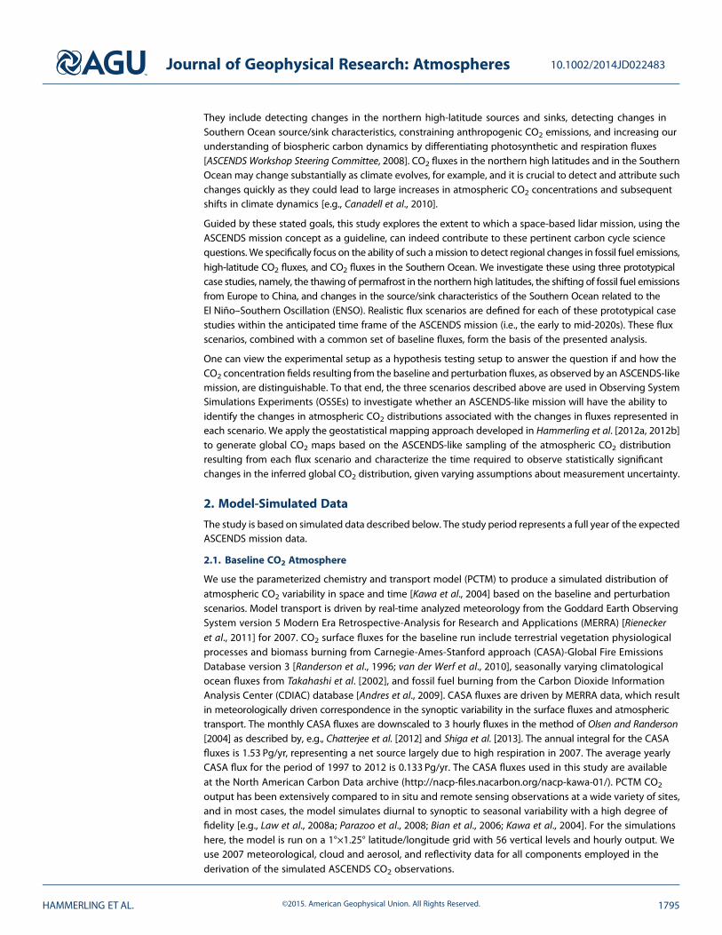
The examined fossil fuel emission perturbations lead to a pronounced spatial signature that is localized overEurope and China (Figures 2c, 2g, 2d, and 2h and Figures S2 and S3 in the supporting information). This is incontrast to the other two experiments (see Figures 1d and 3d), where the detailed spatial signatures are largelylost and especially the yearly signals represent primarily zonal increases. In addition, the magnitude of thelower fossil fuel perturbation signal is very low, which, combined with its small spatial extent, renders the weakfossil fuel signal the most difficult to detect among the investigated scenarios. This exemplifies the challengeof detecting small and localized flux changes from satellite observations.

The highly localized nature of the signal over Europe and China suggests that changes in fluxes would bedetectable and attributable to a given region even if these fluxes were not offset by a corresponding shift inemissions within a similar latitudinal range. It is interesting to observe the different dispersion patterns ofthe European and Chinese emissions, especially when considering their latitudinal range. The effect on theatmospheric concentrations of the European emissions can be observed from equatorial Africa to the Arctic,whereas the range of the Chinese emissions is more limited to their originating latitudinal band (see Figure 2h).

Figure 6. Results for the fossil fuel experiments for medium measurement noise. (first row) The 3month mapped CO2signal (3month mapped). (second row) The significance of the 3month mapped CO2 signal (3 month signific). (third row)The yearlymapped CO2 signal (yearly mapped). (fourth row) The significance of the yearly mapped CO2 signal (yearly signific).The mapped signal is the difference between the mapped perturbation CO2 concentration and the mapped baseline CO2concentration. The significance is the mapped signal divided by the uncertainty of the mapped signal. The values arediscretized for improved visualization. The yellow, orange, and dark red (light, medium, and dark blue) represent areaswhere the mapped perturbation concentration is larger (smaller) than the mapped baseline concentration by more thanone, two, or three standard deviations, respectively, of the uncertainty of the mapped signal. The 3month period is Augustthrough September.

Journal of Geophysical Research: Atmospheres 10.1002/2014JD022483

HAMMERLING ET AL. ©2015. American Geophysical Union. All Rights Reserved. 1803

Given the relative lack of seasonality inthe fossil fuel perturbation scenarios,averaging over longer periods of timeleads to better detectability (Figure 6).Although atmospheric transport clearlyplays a role, the atmospheric signalremains indicative of the source regionof the perturbation flux throughout theseasons. Figure 6h, for example, showsevidence that both the source anddownwind regions of the emissions havea significant signature in the atmosphere.

The effect of varying measurementnoise levels on the detectability is againas expected; increasing measurementnoise leads to decreased significance inthe results and requires in turn longeraveraging periods. For the higher signal,all three noise levels capture the signal inthe yearly results, which is not the casefor the lower signal, where only the noerror case clearly captures the signal(Figure S6 in the supporting information).There is some evidence that a significantsignal is detectable in the yearly mediumand high-error measurement noisecases (Figure 6), and given the nature ofthe signal discussed above, the signalis expected to appear more clearlywhen averaging over periods exceeding1 year. Overall, these findings implythat ASCENDS can in principle detectanthropogenic signal components, butdepending on the strength of the signal,detection might require multiple years.It is hence feasible that ASCENDS canserve to validate anthropogenic emissionchanges over the course of its missionbut is likely not ideal as the primarymonitoring tool for such flux changes.

4.3. Detectability of Changesin Southern Ocean Fluxes

The detection of changes in the SouthernOcean source/sink characteristics is

challenging as a result of a confluence of different factors. The overall magnitude of the signal in theSouthern Oceans is rather weak, with the absolute value of the signal never exceeding 0.4 ppm in thecolumn. In addition, this scenario involves subseasonal and subregional scale flux variability that issuperimposed on a seasonal pattern in the fluxes (Figure S4 in the supporting information). Atmosphericmixing also plays a role insofar as it obscures the Southern Ocean as the origin of the signal as was alsoobserved in the permafrost carbon release scenario. However, applying the remedy of using a shorteraveraging period before atmospheric mixing hides the origin of the signal is not as clear-cut for theSouthern Ocean scenario, because the overall signal is weaker. Spatial gradients associated with the

Figure 7. Results for the Southern Ocean experiment for mediummeasurement noise. (a) The 3month mapped CO2 signal (3monthmapped), (b) significance of the 3month mapped CO2 signal (3monthsignific), (c) yearlymapped CO2 signal (yearlymapped), and (d) significanceof the yearly mapped CO2 signal (yearly signific). The mapped signal isthe difference between the mapped perturbation CO2 concentration andthe mapped baseline CO2 concentration. The significance is the mappedsignal divided by the uncertainty of the mapped signal. The values arediscretized for improved visualization. The yellow, orange, and dark red(light, medium, and dark blue) represent areas where the mappedperturbation concentration is larger (smaller) than the mapped baselineconcentration by more than one, two, or three standard deviations,respectively, of the uncertainty of the mapped signal. The 3month periodis April through June.

Journal of Geophysical Research: Atmospheres 10.1002/2014JD022483

HAMMERLING ET AL. ©2015. American Geophysical Union. All Rights Reserved. 1804

Southern Ocean flux perturbation are most evident in the spring and early summer (Figure 3). Later in theyear, although the concentration signal is stronger, the concentration increase has spread poleward and isless attributable to the Southern Ocean.

For all measurement noise setups, the yearly results clearly indicate a zonal increase in the high southernlatitudes (Figure 7 and Figure S8 in the supporting information). However, it is less clear whether the patternis indicative of the Southern Ocean being the source region within the zonal band. The spatial pattern ofthe 3month results (Figure 7b) is more indicative of the Southern Ocean as the source region, but thesignificance levels are not very high. The most beneficial approach for the Southern Ocean scenario appearsto be conducting analyses over periods of multiple lengths and drawing conclusions from the joint pictureemerging from these analyses. In summary, ASCENDS can detect a Southern Ocean signal representativeof differences due to natural variability in the ENSO climatic mode. ASCENDS may provide a uniquemeasurement view of these regions because the pervasive cloudiness and low sun angles present difficultconditions for passive satellite CO2 sensors. Due to the low-magnitude and small-scale variability within thefluxes giving rise to the signal, however, attributing the signal to specific ocean regions or biogeophysicalprocesses will likely require additional corroborative information.

5. Conclusions

This work assesses the degree to which ASCENDS, a planned lidar CO2 observing satellite mission, cancontribute to the detection of three types of CO2 flux change scenarios relevant to global carbon cyclescience: the release of carbon due to the thawing of permafrost in the northern high latitudes, the shiftingof fossil fuel emissions from Europe to China, and ENSO-related changes in the source/sink characteristicsin the Southern Ocean. These three scenarios were used to design OSSEs for signal detection studies toinvestigate if the ASCENDS mission has the ability to detect the unfolding of these scenarios compared to abaseline scenario. Two different levels of measurement noise and a no-measurement noise reference caseswere investigated.

This study is based on a number of simplifications. For each scenario, the only flux component that is varied isthe flux component under investigation, while all other fluxes are fixed. In reality, many changes might occursimultaneously, and the resulting CO2 concentration signal patterns might overlap, which makes signaldetection more challenging. We have introduced some additional variability by sampling and mapping thebaseline concentration field rather than assuming a static baseline concentration field in the comparisonprocedure, however, that might not be equivalent to, for example, having misspecified biospheric fluxes.Such misspecifications could be aliased with the true signals and misleading signal patterns could occur. Thiscould impact the conclusions of this study insofar that it would be more difficult to link detectable signalswith the underlying change in fluxes.

The results indicate that the ASCENDS mission can in principle detect the types of signals investigated in thisstudy. The permafrost thawing flux perturbation is readily detectable at a high level of significance. Spatialgradients, which are of great interest for process attribution, were best detected using 2 or 3month aggregationperiods in the late spring/early summer. For the Southern Ocean scenario, differences due to the naturalvariability in the ENSO climatic mode were primarily detectable as a zonal increase. The relative magnitude ofthe signal, however, is much smaller than the permafrost-thawing signal. Spatial and temporal high-frequencychanges in the anomaly fluxes produce additional variability in the signal, making detection of more detailedgradients than a zonal increase challenging for the Southern Ocean scenario. Conducting analyses overperiods of varying lengths and analyzing them jointly provide a possible diagnostic strategy.

The fossil fuel emission detectability is directly related to the strength of the signal and the level ofmeasurement noise. As is true for all scenarios, the effect of varying measurement noise levels is asexpected: increasing measurement noise levels leads to decreased significance in the results and requiresin turn longer averaging periods. For the nominal (lower) fossil fuel emission signal, only the noise-freeinstrument test produces a clearly detectable signal, while all three noise levels capture the higher(exaggerated) signal case. The emergence of a detectable signal suggests that averaging over periodslonger than the 1 year period considered in this study would also render signals of the magnitude of thelower fossil fuel emission signal detectable.

Journal of Geophysical Research: Atmospheres 10.1002/2014JD022483

HAMMERLING ET AL. ©2015. American Geophysical Union. All Rights Reserved. 1805

All in all, the expected precision and sampling characteristics of ASCENDS promise to substantially enhanceour ability to detect variations in CO2 fluxes and to inform the mechanisms that control them. Future workincludes comparing the signal detection performance of ASCENDS to passive sensors, which might beemployed within the time frame of the ASCENDS mission. Additional future work entails a comprehensivestudy of the effect of uncertainties in fluxes other than those defining the signal on the detectability of thesignal, for example, by using an ensemble of biospheric fluxes to vary the baseline fluxes.

ReferencesAbshire, J. B., H. Riris, G. R. Allan, C. J. Weaver, J. Mao, X. Sun, W. E. Hasselbrack, S. R. Kawa, and S. Biraud (2010), Pulsed airborne lidar

measurements of atmospheric CO2 column absorption, Tellus B, 62, 770–783, doi:10.1111/j.1600-0889.2010.00502.x.Andres, R. J., T. A. Boden, and G. Marland (2009), Monthly Fossil-Fuel CO2 Emissions: Mass of Emissions Gridded by One Degree Latitude by

One Degree Longitude, Carbon Dioxide Information Analysis Center, Environmental Sciences Division, Oak Ridge National Laboratory,Oak Ridge, Tenn., 37831-6290.

Andres, R. J., J. S. Gregg, L. Losey, G. Marland, and T. A. Boden (2011), Monthly, global emissions of carbon dioxide from fossil fuel consumption,Tellus B, 63, 309–327, doi:10.1111/j.1600-0889.2011.00530.x.

ASCENDS Workshop Steering Committee (2008), Active Sensing of CO2 Emissions over Nights, Days, and Seasons (ASCENDS) Mission NASAScience Definition and Planning Workshop Report, 1–78.

Baker, D. F., H. Bösch, S. C. Doney, D. O’Brien, and D. S. Schimel (2010), Carbon source/sink information provided by column CO2measurementsfrom the orbiting carbon observatory, Atmos. Chem. Phys., 10, 4145–4165, doi:10.5194/acp-10-4145-2010.

Bian, H., S. R. Kawa, M. Chin, S. Pawson, Z. Zhu, P. Rasch, and S. Wu (2006), A test of sensitivity to convective transport in a global atmosphericCO2 simulation, Tellus B, 58, 463–475, doi:10.1111/j.1600-0889.2006.00212.x.

Brown, J., O. J. Ferrians Jr., J. A. Heginbottom, and E. S. Melnikov (1998), Circum-arctic map of permafrost and ground ice conditions, Natl.Snow and Ice Data Cent., Digital media, Boulder, Colo. [Revised February 2001.]

Canadell, J. G., C. L. Quéré, M. R. Raupach, C. B. Field, E. T. Buitenhuis, P. Ciais, T. J. Conway, N. P. Gillett, R. A. Houghton, and G. Marland (2010),Carbon sciences for a new world, Curr. Opin. Environ. Sustainability, 2.

Chatterjee, A., A. M. Michalak, J. L. Anderson, K. L. Mueller, and V. Yadav (2012), Toward reliable ensemble Kalman filter estimates of CO2 fluxes,J. Geophys. Res., 117, D22306, doi:10.1029/2012JD018176.

Crisp, D., et al. (2004), The Orbiting Carbon Observatory (OCO) mission, Adv. Space Res., 34, 700–709, doi:10.1016/j.asr.2003.08.062.Disney, M. I., P. E. Lewis, M. Bouvet, A. Prieto-Blanco, and S. Hancock (2009), Quantifying surface reflectivity for spaceborne lidar via two

independent methods, IEEE Trans. Geosci. Remote Sens., 47, 3262–3271.Doney, S. C., I. Lima, R. A. Feely, D. M. Glover, K. Lindsay, N. Mahowald, J. K. Moore, and R.Wanninkhof (2009), Mechanisms governing interannual

variability in upper-ocean inorganic carbon system and air-sea CO2 fluxes: Physical climate and atmospheric dust, Deep Sea Res., Part II,56(8–10), 640–655, doi:10.1016/j.dsr2.2008.12.006.

Ehret, G., C. Kiemle, M. Wirth, A. Amediek, A. Fix, and S. Houweling (2008), Space-borne remote sensing of CO2, CH4, and N2O by integratedpath differential absorption lidar: A sensitivity analysis, Appl. Phys. B, 90, 593–608, doi:10.1007/s00340-007-2892-3.

Field, C. B., J. Sarmiento, and B. Hales (2007), The carbon cycle of North America in a global context, in The First State of the Carbon CycleReport (SOCCR): The North American Carbon Budget and Implications for the Global Carbon Cycle. A Report by the U.S. Climate Change ScienceProgram and the Subcommittee on Global Change Research, edited by A. W. King et al., pp. 21–28, Natl. Oceanic and Atmos. Admin., Natl.Clim. Data Cent., Asheville, N. C.

Gruber, N., et al. (2009), Oceanic sources, sinks, and transport of atmospheric CO2, Global Biogeochem. Cycles, 23, GB1005, doi:10.1029/2008GB003349.

Hammerling, D. M., A. M. Michalak, and S. R. Kawa (2012a), Mapping of CO2 at high spatiotemporal resolution using satellite observations:Global distributions from OCO-2, J. Geophys. Res., 117, D06306, doi:10.1029/2011JD017015.

Hammerling, D. M., A. M. Michalak, C. O’Dell, and S. R. Kawa (2012b), Global CO2 distributions over land from the Greenhouse Gases ObservingSatellite (GOSAT), Geophys. Res. Lett., 39, L08804, doi:10.1029/2012GL051203.

Hu, Y., et al. (2008), Sea surface wind speed estimation from space-based lidar measurements, Atmos. Chem. Phys., 8, 3593–3601,doi:10.5194/acp-8-3593-2008.

Kawa, S. R., D. J. Erickson III, S. Pawson, and Z. Zhu (2004), Global CO2 transport simulations using meteorological data from the NASA dataassimilation system, J. Geophys. Res., 109, D18312, doi:10.1029/2004JD004554.

Kawa, S. R., J. Mao, J. B. Abshire, G. J. Collatz, X. Sun, and C. J. Weaver (2010), Simulation studies for a space-based CO2 lidar mission, Tellus B,62, 759–769, doi:10.1111/j.1600-0889.2010.00486.x.

Kiemle, C., S. R. Kawa, M. Quatrevalet, and E. V. Browell (2014), Performance simulations for a spaceborne methane lidar mission, J. Geophys.Res. Atmos., 119, 4365–4379, doi:10.1002/2013JD021253.

Kuze, A., H. Suto, M. Nakajima, and T. Hamazaki (2009), Thermal and near infrared sensor for carbon observation Fourier-transformspectrometer on the greenhouse gases observing satellite for greenhouse gases monitoring, Appl. Opt., 48, 6716–6733,doi:10.1364/AO.48.006716.

Law, R. M., et al. (2008a), TransCom model simulations of hourly atmospheric CO2: Experimental overview and diurnal cycle results for 2002,Global Biogeochem. Cycles, 22, GB3009, doi:10.1029/2007GB003050.

Law, R. M., R. J. Matear, and R. J. Francey (2008b), Comment on saturation of the Southern ocean CO2 sink due to recent climate change,Science, 319, 570.

Le Quéré, C., M. R. Raupach, J. G. Canadell, and E. A. Marland (2009), Trends in the sources and sinks of carbon dioxide,Nat. Geosci., 2, 831–836.Lemke, P., et al. (2007), Changes in snow, ice and frozen ground, in Climate Change 2007: The Physical Science Basis: Contribution of Working

Group I to the Fourth Assessment Report of the Intergovernmental Panel on Climate Change, edited by S. Solomon et al., Cambridge Univ. Press,Cambridge, U. K.

Mao, J., and S. R. Kawa (2004), Sensitivity studies for space-based measurement of atmospheric total column carbon dioxide by reflectedsunlight, Appl. Opt., 43, 914–927.

Meredith, M. P., A. C. N. Garabato, A. M. Hogg, and R. Farneti (2012), Sensitivity of the overturning circulation in the southern ocean to decadalchanges in wind forcing, J. Clim., 25, 99–110.

AcknowledgmentsThis material is based upon worksupported by the National Aeronauticsand Space Administration under grantNNX08AJ92G issued through theResearch Opportunities in Spaceand Earth Sciences Carbon CycleScience program and by Jet PropulsionLaboratory subcontract 1442785 as well asthe ASCENDS Science RequirementsDefinition Team. S. Doney acknowledgessupport from U.S. National ScienceFoundation (AGS-1048827). K. Schaeferacknowledges support from the NationalOceanic and Atmospheric Administrationunder grant NA09OAR4310063 and fromthe National Aeronautics and SpaceAdministration under grant NNX10AR63G.All the data used in this study can berequested by emailing Dorit Hammerling(dorith@ucar.edu). We thank RobertAndres for providing CDIAC fossil fuelemissionfluxes and his advice in applyingthem. We thank Ivan Lima for his supportwith the Southern Ocean fluxes andMichael Manyin and Yuping Liu forexecuting PCTM model runs.

Journal of Geophysical Research: Atmospheres 10.1002/2014JD022483

HAMMERLING ET AL. ©2015. American Geophysical Union. All Rights Reserved. 1806

National Research Council (2007), Earth Science and Applications From Space: National Imperatives for the Next Decade and Beyond, 456 pp.,The National Acad. Press, Washington, D. C. 20001.

Olivier, J., G. Janssens-Maenhout, and J. Peters (2012), Trends in Global CO2 Emissions; 2012 Report, PBL Netherlands Environmental AssessmentAgency; Ispra: Joint Research Centre, The Hague, Netherlands.

Olsen, S. C., and J. T. Randerson (2004), Differences between surface and column atmospheric CO2 and implications for carbon cycle research,J. Geophys. Res., 109, D02301, doi:10.1029/2003JD003968.

Parazoo, N. C., A. S. Denning, S. R. Kawa, K. D. Corbin, R. S. Lokupitiya, and I. T. Baker (2008), Mechanisms for synoptic variations of atmosphericCO2 in North America, South America and Europe, Atmos. Chem. Phys., 8, 7239–7254.

Peters, G. P., G. Marland, C. L. Quéré, T. Boden, J. G. Canadell, and M. R. Raupach (2011), Rapid growth in CO2 emissions after the 2008–2009global financial crisis, Nat. Clim. Change, 2, 2–4.

Randerson, J. T., M. V. Thompson, C. M. Malmstrom, C. B. Field, and I. Y. Fung (1996), Substrate limitations for heterotrophs: Implications formodels that estimate the seasonal cycle of atmospheric CO2, Global Biogeochem. Cycles, 10(4), 585–602, doi:10.1029/96GB01981.

Rienecker, M. M., et al. (2011), MERRA: NASA’s Modern-Era retrospective analysis for research and applications, J. Clim., 24, 3624–3648.Schaaf, C. B., et al. (2002), First operational BRDF, albedo nadir reflectance products from MODIS, Remote Sens. Environ., 83(1–2), 135–148,

doi:10.1016/S0034-4257(02)00091-3.Schaefer, K., G. J. Collatz, P. Tans, A. S. Denning, I. Baker, J. Berry, L. Prihodko, N. Suits, and A. Philpott (2008), combined simple biosphere/

Carnegie-Ames-Stanford approach terrestrial carbon cycle model, J. Geophys. Res., 113, G03034, doi:10.1029/2007JG000603.Schaefer, K., T. Zhang, L. Bruhwiler, and A. P. Barrett (2011), Amount and timing of permafrost carbon release in response to climate warming,

Tellus B, 63, 165–180, doi:10.1111/j.1600-0889.2011.00527.x.Shiga, Y. P., A. M. Michalak, S. R. Kawa, and R. J. Engelen (2013), In-situ CO2 monitoring network evaluation and design: A criterion based on

atmospheric CO2 variability, J. Geophys. Res. Atmos., 118, 2007–2018, doi:10.1002/jgrd.50168.Spiers, G. D., R. T. Menzies, J. Jacob, L. E. Christensen, M. W. Phillips, Y. Choi, and E. V. Browell (2011), Atmospheric CO2 measurements with a

2 μm airborne laser absorption spectrometer employing coherent detection, Appl. Opt., 50, 2098–2111, doi:10.1364/AO.50.002098.Takahashi, T., et al. (2002), Global sea-air CO2 flux based on climatological surface ocean pCO2, and seasonal biological and temperature

effects, Deep Sea Res., Part II, 49(9–10), 1601–1622, doi:10.1016/S0967-0645(02)00003-6.Tarnocai, C., J. G. Canadell, E. A. G. Schuur, P. Kuhry, G. Mazhitova, and S. Zimov (2009), Soil organic carbon pools in the northern circumpolar

permafrost region, Global Biogeochem. Cycles, 23, GB2023, doi:10.1029/2008GB003327.van der Werf, G. R., J. T. Randerson, L. Giglio, G. J. Collatz, M. Mu, P. S. Kasibhatla, D. C. Morton, R. S. DeFries, Y. Jin, and T. T. van Leeuwen (2010),

Global fire emissions and the contribution of deforestation, savanna, forest, agricultural, and peat fires (1997–2009), Atmos. Chem. Phys., 10,11,707–11,735, doi:10.5194/acp-10-11707-2010.

Yokota, T., Y. Yoshida, N. Eguchi, Y. Ota, T. Tanaka, H. Watanabe, and S. Maksyutov (2009), Global concentrations of CO2 and CH4 retrievedfrom GOSAT: First preliminary results, SOLA, 5, 160–163, doi:10.2151/sola.2009-041.

Zhang, T., R. G. Barry, K. Knowles, J. A. Heginbottom, and J. Brown (1999), Statistics and characteristics of permafrost and ground-icedistribution in the Northern Hemisphere, Polar Geogr., 23(2), 132–154.

Zimov, S. A., E. A. G. Schuur, and F. S. Chapin III (2006), Permafrost and the Global Carbon Budget, Science, 312(5780), 1612–1613, doi:10.1126/science.1128908, 16 June.

Journal of Geophysical Research: Atmospheres 10.1002/2014JD022483

HAMMERLING ET AL. ©2015. American Geophysical Union. All Rights Reserved. 1807