detecting problems in survey data using benford’s · pdf filedetecting problems in...

Detecting Problems in Survey Data using

Benford’s Law∗

George JudgeUniversity of California at Berkeley†

Laura SchechterUniversity of Wisconsin at Madison‡

November 1, 2007

Abstract

It is 15:00 in Nairobi. Do you know where your enu-merators are??

Good quality data is paramount for applied economic research. Ifthe data are distorted, corresponding conclusions may be incorrect.We demonstrate how Benford’s law, the distribution that first digitsof numbers in certain data sets should follow, can be used to test fordata abnormalities. We conduct an analysis of nine commonly useddatasets and find that much data from developing countries is of poorquality while data from the US seems to be of uniformly better qual-ity. Female and male respondents give data of similar quality.Keywords: Benford’s law, first-digit phenomenon, relative frequen-cies, expected frequencies, data errors, survey quality.AMS Classification: Primary 62E20.JEL classification: C10, C24.

∗The order of the authors’ names has only alphabetical significance. We have benefitedfrom helpful comments from Jennifer Alix-Garcia, Wendy Cho, Joanne Lee, Ted Miguel,Michael Roberts, Elisabeth Sadoulet, two anonymous referees, and seminar participants atBREAD, Purdue, and UW Madison. John Morrow provided excellent research assistanceand also created the convenient utility to test your own data against Benford’s law whichcan be found at http://www.checkyourdata.com. The second author received funding fromUSDA Hatch grant 142-1038.

†Professor in the Graduate School, Berkeley CA. e-mail: [email protected].‡Agricultural and Applied Economics, Madison WI. e-mail: [email protected].

1

1 Introduction

In developing countries, much of the social and economic data are collectedby surveys. Horror stories are common in which, somebody discovers that one(or more) enumerator is answering the survey himself rather than actuallyinterviewing households. Also prevalent are stories in which, after spendinga large sum of money to buy a data set, a researcher realizes that the infor-mation of interest to him seems inaccurate. Since information contained insurvey data often plays a key role in policy decisions, it is important to havea basis for identifying its quality. 1

In data obtained from economic surveys, questions usually arise pertain-ing to: i) the quality of the enumerators (what if an enumerator completesthe survey questionnaire while enjoying coffee at Starbucks?) and ii) thequality of the responses from those interviewed (what if the questionnaire ispoorly designed and elicits answers from respondents that are inconsistentwith the objectives of the question?). If either the error of omission or com-mission occurs, it would be useful to identify it early in the research process.Therefore, a basis upon which one could recognize survey data irregularities,manipulated outcomes, and abnormal digit and number occurrences, wouldbe a valuable tool for researchers designing and using survey data. In thispaper, we demonstrate, in the context of large data sets, the use of Benford’sfirst significant digit (FSD) law as one such possibility.2

1.1 Benford’s Law

Benford’s law characterizes the distribution of FSD observed in large sets ofdata. In 1881 Simon Newcomb observed that numbers with a first digit of 1were observed more often than those starting with 2, 3, and so on. Newcombwas able to calculate the probability of a number having a particular nonzerofirst digit and published this in an article in The American Journal of Math-

ematics. Benford, unaware of Newcomb’s article, made the same observation

1Philipson & Malani (1999) posit that economists tend to pay more attention to theconsumption of data rather than the production of data. This is evidenced by the largeliterature on how to deal with measurement error and the relatively small literature onhow to prevent it. The three volumes edited by Grosh & Glewwe (2000), in addition tobooks by Groves (1989), Sudman et al. (1996), and Biemer et al. (1991) synthesize much ofthe literature and accepted best practice with regards to survey design and data collection.

2The first significant digit is the first non-zero digit reading a number from left to right.

2

and published an article in The Proceedings of the American Philosophical

Society in 1938. This FSD phenomenon was christened as Benford’s law.Newcomb observed the probability of a number having a particular non-

zero first digit as roughly

P (First digit is d) = log10(1 +1

d) (1)

where d = 1, 2, . . . , 9. This formula produces a monotonically decreasingFSD distribution and suggests that the quantities expressed in base 10 willbe uniformly distributed on a logarithmic scale. Using Newcomb’s formula,the probability that the first digit of a number is 1 is about thirty percent(P (d = 1) = log10(1 + 1

1) = log10(2) ≈ .30) while the probability the first

digit is 9 is 4.6 percent. Benford’s law also has the nice property that itsatisfies a scale and base invariance condition (Raimi 1976, Pietronero et al.2001). This condition means that multiplying the data, such as prices orquantities of farm output, by any positive scalar will lead to the same FSDprobability distribution.

Benford’s somewhat surprising law, with its monotonic decreasing FSDdistribution, has been demonstrated to hold with a large number of datasets that include the populations of towns, budgetary data of corporations,the number of citations received by papers, and the half-lives of radioactiveatoms. The range of applications of the Benford phenomenon is impres-sive. All of these applied FSD distributions represent a dynamic mixture ofdata outcomes whose resulting combination is unrestricted in terms of thepossibility of spanning the nine digit space.

Of course, not all natural data sets can be captured by the Benford FSDdistribution. Binary or categorical data are two important economic exam-ples that often occur in surveys. The daily closing price of a particular mutualfund on the Canadian Stock Exchange over a six month period is anotherexample when Benford might not be expected to hold. On the other hand, inline with the dynamic mixture condition noted above, the FSD distributionof the closing prices for 500 stocks on this exchange over a six month periodshould, and does almost perfectly, track Benford.

Many data sets that fulfill the mixture-combination data condition notedabove do not closely follow Benford. In fact, half of Benford’s data sets donot closely follow his FSD distribution in terms of the level of the function.However, these data sets are Benford-like in that they are monotonic decreas-ing functions of the FSD data. Building on this base, we use the Benford

3

monotonic decreasing FSD distribution as one basis for identifying FSD dis-tributions that may involve possible tampering or falsification of the datain economic surveys. Basically, it is difficult through tampering or humaninfluence to duplicate the FSD’s from natural outcomes of data sets, a factwe hope to exploit in this paper.

Like the equally surprising golden ratio (Livio 2002), theories abound asto the basis of the first-digit phenomenon. Consequently, there have beenmany attempts over the years to explain the logarithmic formula and to pro-vide a theoretical basis for the observed phenomenon. Hill (1995) provideda statistical derivation of the law in the form of a Central Limit Theoremfor significant digits: “If distributions are selected at random and randomsamples are taken from each of these distributions, the significant first digitsof the combined sample will converge to the logarithmic (Benford) distri-bution.” For overviews of the history and a sampling of the theoretical andempirical results, the reader is directed to Raimi (1976), Diaconis (1977),Schatte (1988), Hill (1995), Rodriguez (2004), Hill & Schurger (2005) andBerger & Hill (2007).

1.2 Overview of the Paper

Building on Benford’s monotonic decreasing FSD distribution for naturallyoccurring multiplicative data sets, our objective is to exhibit scale-invariantdata that may be expected to obey Benford’s law and evaluate the behavioralbasis of departures.3 Others who have used Benford’s law to check the valid-ity of purported scientific data in the social sciences include Varian (1972),Carslaw (1988), Nigrini (1996), Durtschi et al. (2004), Geyer & Williamson(2004), de Marchi & Hamilton (2006), Giles (2007) and Nye & Moul (2007).

To illustrate the use of Benford’s FSD law to evaluate enumerator andrespondent performance, we carry out a detailed analysis on survey data fromrural Paraguayan households. Using this data we find that some enumeratorsand questions yield higher quality responses than others. We also comparedata on crops which are more important for a household’s income (withimportance defined in multiple ways) with data on less important crops. Wefind that the former are fairly well in accord with Benford’s law, while thelatter are much less so. This suggests that Benford’s FSD law holds whencrop quantities are more salient and so farmers are able to provide their

3For some formal characterizations of when scale invariance occurs, see Morrow (2007).

4

answers with more accuracy.In addition, we conduct a less detailed analysis of nine household surveys

across the globe used extensively by research economists, presenting evidencethat several widely used household data sets in development economics arenot of very high quality. We find this is especially true of the Progresa datafrom Mexico. On the other hand, the data from the United States seems tobe of uniformly better quality than a range of surveys from the eight lessdeveloped countries. This may be because farmers in the US consult theirrecords when responding to survey questionnaires or because they are moresure of exact quantities. We also find that the quality of data reported byfemale and male respondents is not very different.

We have access to one data set with data from some clusters which werelater suspected to be falsified. These data are less in accord with Benford’slaw. On the other hand, we have another data set in which enumeratorswere asked to express their opinion regarding the quality of the data. Whenthey opine that the quality was not good, the data is no less in accordwith Benford’s law. Perhaps this is because the natural FSD data processunderlying Benford’s law (like the heads or tails distribution in the flippingof a coin) is hard to duplicate. When an enumerator fakes data in an attemptto make it look real, and when he opines that some data is of better quality,this is exactly the data which is less in accord with Benford, not more.

The paper is organized as follows: Section 2 discusses the Paraguayandata used in this paper and applies Benford’s law to both the 2002 and1999 rounds of data; Section 3 expands the analysis to compare data setsfrom around the globe; Section 4 discusses the implications of our resultsfor theory and practice; and Section 5 summarizes. Appendix A contains amore detailed description of the online utility www.checkyourdata.com whichpeople can use to carry out the tests shown in this paper. Appendix Bcontains extra tables.

2 Paraguayan Survey Data

To illustrate the usefulness of Benford’s law in assessing data integrity we usesurvey data from rural Paraguay. We find that some survey questions elicitmore errors than others. For example, questions for which farmers know theexact answer generally conform to Benford’s law while questions for whichfarmers may be unsure of the exact answer do not. When unsure, respondents

5

are more likely to choose numbers starting with 5 than Benford’s law wouldsuggest. Finally, questions about which farmers may have an incentive to hidethe truth, such as their donations to church, do not conform with Benford’slaw. We also show that data collected by some enumerators are in accordwith Benford’s law while data collected by others are not.

In 1991, the Land Tenure Center at the University of Wisconsin in Madi-son and the Centro Paraguayo de Estudios Sociologicos in Asuncion workedtogether in the design and implementation of a survey of 300 rural Paraguayanhouseholds in 16 villages in three departments (comparable to states). Thesampling design resulted in a random sample, stratified by land-holdings.The original survey was followed by subsequent rounds of data collection in1994, 1999, and 2002. Summary statistics about both the households andthe respondents can be found in Table B-1.

2.1 Benford’s Law Applied to 2002 Paraguay Data

2.1.1 Enumerated Data

We now examine whether the data collected in Paraguay produces an FSDdistribution that is consistent with Benford’s law. We look at data for whichthe enumerator directly recorded the answer as stated by the farmer. Thefarmer was asked how much of each crop was harvested by his household inthe past year.4 The data in Table 1 indicates how the data compares withBenford’s law. From a review of the table, it appears the data generallyconform to Benford’s law, although quantities with an FSD of 5 are muchmore common than suggested by Benford’s law.5

In addition to merely visually reviewing the data, we use a χ2 goodness-of-fit test to check the extent to which the data conforms with Benford’s law.The χ2 statistic is calculated as χ2 =

∑9i=1

(ei−bi)2

bi

with 8 degrees of freedomwhere ei is the observed frequency in each bin in the empirical data and bi

is the frequency expected by Benford. The 10%, 5%, and 1% critical valuesfor χ2 are 13.36, 15.51, and 20.09.

Following Giles (2007), we use Kuiper’s modified Kolmogorov-Smirnov

4If a household produces 150 kilos of corn and 420 kilos of cassava that will count asFSDs of 1 and 4, not 5.

5de Marchi & Hamilton (2006) use Benford’s law to test for tampering in self-reportedtoxics emissions by firms and likewise find that there are a disproportionate share ofquantities beginning with 5.

6

Table 1: Benford’s Law and Production Quantities

Variable Obs. 1 2 3 4 5 6 7 8 9Benford 30.10 17.61 12.49 9.69 7.92 6.69 5.80 5.12 4.58All Products 1632 31.50 19.30 12.81 7.90 12.93 5.82 4.11 3.62 2.02Enumerator 1 516 30.23 19.19 13.37 8.72 10.66 8.91 2.71 4.46 1.74Enumerator 2 556 32.73 19.06 12.59 7.73 12.77 6.29 3.42 3.42 1.98Enumerator 3 560 31.43 19.64 12.50 7.32 15.18 2.50 6.07 3.04 2.32P.I. sat in 582 33.33 16.49 13.06 7.04 13.92 4.64 4.47 4.64 2.41P.I. didn’t sit in 1050 30.48 20.86 12.67 8.38 12.38 6.48 3.90 3.05 1.81

goodness-of-fit test (VN) because it recognizes the ordinality and circularityof the data. This means that first digits of 5 and 6 are close to one another, asare first digits of 9 and 1. Kuiper’s test does not depend on the choice of origin(in contrast to the typical Kolmogorov-Smirnov test). Kuiper’s VN statisticis calculated as VN = maxx[Fe(x)−Fb(x)]+maxx[Fb(x)−Fe(x)] where Fe(x)is the empirical CDF of the FSD distribution and Fb(x) is Benford’s CDF.Critical values for a modified Kuiper test (V ∗

N = VN [N1/2+0.155+0.24N−1/2])have been given by Stephens (1970). However, both the original and modifiedKuiper tests were designed for use with continuous distributions. We use10%, 5%, and 1% critical values for V ∗

N of approximately 1.19, 1.32, and 1.58shown by Morrow (2007) to be asymptotically valid.

In addition to the two statistical tests, we also include four measures ofthe distance between the empirical data and Benford’s distribution whichare outside of the hypothesis-testing framework and insensitive to samplesize. We include the Pearson correlation coefficient between the empiricalproportions of first digits in the data and those predicted by Benford. Ad-ditionally, as suggested by Leemis et al. (2000), we calculate the distancemeasure m = maxi=1,2,...,9{|bi − ei|}. Third, as suggested by Cho & Gaines(2007) we include a measure which is based on the Euclidean distance be-

tween the two distributions. Let d =√

∑9i=1(bi − ei)2. We then divide d by

the maximum possible distance (which would occur when all numbers beginwith an FSD of 9) so that the value is bounded between 0 and 1 and we callthat measure d∗. Lastly, we note that the mean of the first digits in Benford’sFSD distribution is 3.4402. The maximum possible distance to this wouldoccur when all numbers begin with an FSD of 9. We use a distance measurea∗ which is the absolute value of the difference between the average of the

7

Table 2: Correlations (r), the m Statistic, Distances d∗ and a∗, χ2 Tests, andKuiper V ∗

N Tests between Benford’s Law and Production Quantities

Variable r m d∗ a∗ χ2 V ∗N

All Products 0.97 0.050 0.065 0.051 101.34∗∗ 2.69∗∗

Enumerator 1 0.97 0.031 0.057 0.042 28.20∗∗ 1.50∗

Enumerator 2 0.98 0.049 0.070 0.061 37.58∗∗ 1.68∗∗

Enumerator 3 0.94 0.073 0.092 0.050 67.92∗∗ 1.97∗∗

P.I. sat in 0.96 0.060 0.078 0.041 44.94∗∗ 1.47∗

P.I. didn’t sit in 0.97 0.045 0.067 0.057 67.54∗∗ 2.26∗∗

* indicates 95% and ** indicates 99% significantly different from Benford.

empirical FSD distribution and the average of Benford’s FSD distributiondivided by the maximum possible difference.6

The Pearson correlation coefficient between the empirical data and Ben-ford’s distribution tends to be extremely close to 1 for all of the data setswe look at. The level of variation in r is thus too small to make it a veryuseful distance measure. The measure a∗, based on the mean of the firstdigits of the data, is interesting but it is the measure which is most often indisagreement with the other measures and tests. This may be because it isnot based on bi and ei directly as are the other tests. Thus, for our purposes,of the four distance measures we prefer m and d∗.

All of these statistics for testing and measures for summarizing the degreeof deviation from Benford’s law are given in Table 2. The goodness-of-fit testssuggest a rejection of the hypothesis that the data on quantities produced wasgenerated by Benford’s distribution. We might worry that one of the threeenumerators was not completing surveys properly, thus explaining why thequantity data does not conform with Benford’s law. In addition, the PrincipalInvestigator (P.I.) sat in on interviews with a different enumerator every day,alternating among the three. There was no specific type of household theP.I. tended to visit more often. We analyze whether or not the distributionof FSD changes based on the identity of the enumerator and the presence ofthe P.I. during the interview. Results suggest that bias remains.

The relative frequency departures are probably due to the fact that the

6Note that higher values of V ∗N

, χ2, m, d∗, and a∗ imply the empirical data is lesssimilar to Benford’s distribution, while higher values of the correlation r imply the datais more similar to Benford’s distribution.

8

farmers were not always sure exactly how much of a crop they had harvestedand so tended to choose ‘nice’ round numbers, e.g. a farmer is more likely toclaim a harvest of 500 kilos of corn than 422 kilos. From the results in Table 2,we can statistically reject at the 99% level the hypothesis that the productiondata were generated in accord with Benford’s law. One could argue that theoverabundance of observations starting with 5 is not due to guesstimationbut rather to the fact that farmers’ plots are similar sizes and thus generatecrop production of similar amounts. If this were the case, we would expectthat there should also be relatively many observations beginning with 4 and6 as well. However, when looking at the data one can see that this is not thecase - the abundance of 5’s is at the expense of 4’s and 6’s.

This illustrates how Benford’s law may be used to distinguish problemsin survey data arising because of an enumerator from those arising becauseof an ill-phrased question. For researchers who design surveys and collectdata, this situation can be identified early in the survey collection process tohelp avoid major difficulties in subsequent econometric analysis.

2.1.2 Other Variables

In Table 3, we perform the same exercise on other variables which seem likelyto follow Benford’s law. We cannot reject that the data on the number ofanimals owned, and hectares of land owned or used come from Benford’sdistribution. The animals-owned variables include separately the quantitiesowned of each animal species. If households are able to report the assetsthey own more accurately than the quantities of crops harvested, measuresof wealth for rural households in developing countries may be more accuratethan measures of income. For research in which either wealth or incomecan be used, this may suggest a preference for the former. On the otherhand, measures of both income and wealth also require accurate reports ofprices, which may also contain significant error. We reject the hypothesisthat donations to church are in accord with Benford’s law. This may be be-cause respondents are not sure how much they donated to church or becauserespondents are reluctant to answer honestly.

2.2 Benford’s Law Applied to 1999 Paraguay Data

In 2002 only three enumerators collected the Paraguayan survey data, whilein 1999 ten enumerators worked on the survey (with no overlap between the

9

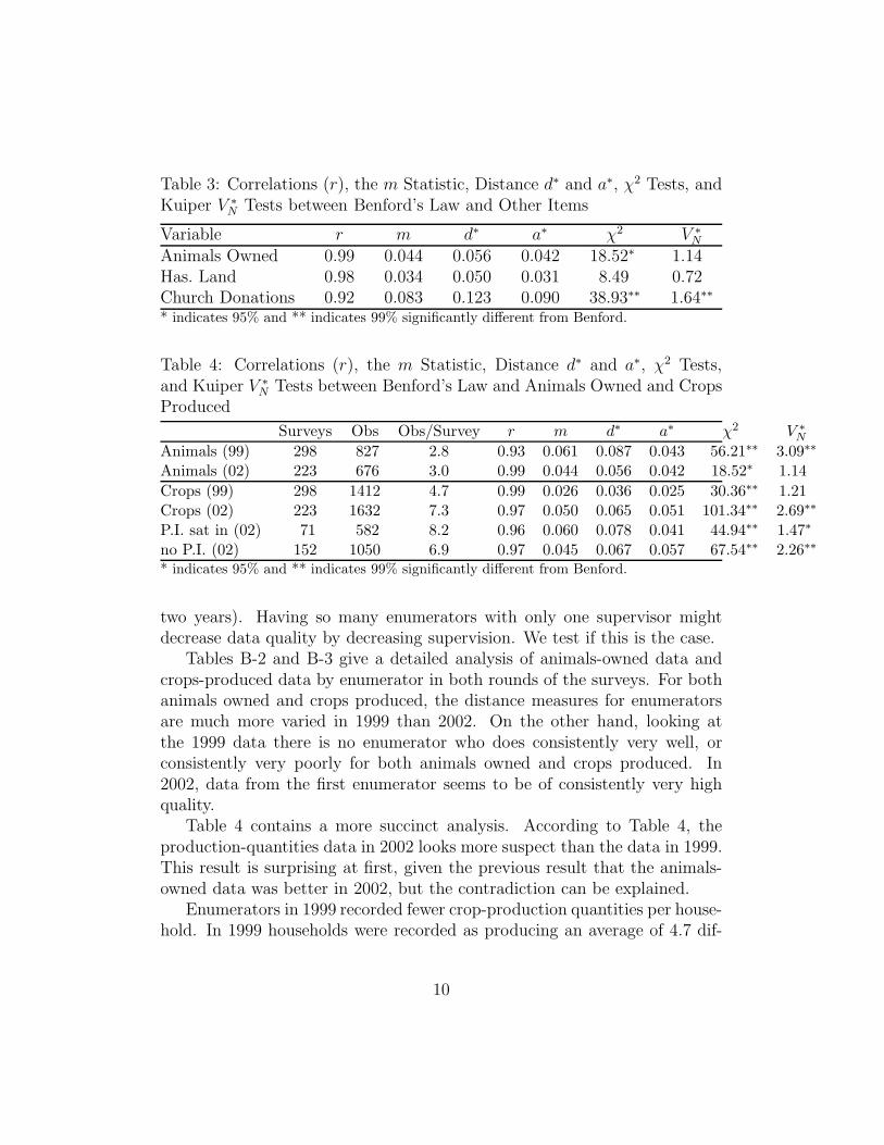
Table 3: Correlations (r), the m Statistic, Distance d∗ and a∗, χ2 Tests, andKuiper V ∗

N Tests between Benford’s Law and Other Items

Variable r m d∗ a∗ χ2 V ∗N

Animals Owned 0.99 0.044 0.056 0.042 18.52∗ 1.14Has. Land 0.98 0.034 0.050 0.031 8.49 0.72Church Donations 0.92 0.083 0.123 0.090 38.93∗∗ 1.64∗∗


Table 4: Correlations (r), the m Statistic, Distance d∗ and a∗, χ2 Tests,and Kuiper V ∗

N Tests between Benford’s Law and Animals Owned and CropsProduced

Surveys Obs Obs/Survey r m d∗ a∗ χ2 V ∗N

Animals (99) 298 827 2.8 0.93 0.061 0.087 0.043 56.21∗∗ 3.09∗∗

Animals (02) 223 676 3.0 0.99 0.044 0.056 0.042 18.52∗ 1.14

Crops (99) 298 1412 4.7 0.99 0.026 0.036 0.025 30.36∗∗ 1.21Crops (02) 223 1632 7.3 0.97 0.050 0.065 0.051 101.34∗∗ 2.69∗∗

P.I. sat in (02) 71 582 8.2 0.96 0.060 0.078 0.041 44.94∗∗ 1.47∗

no P.I. (02) 152 1050 6.9 0.97 0.045 0.067 0.057 67.54∗∗ 2.26∗∗


two years). Having so many enumerators with only one supervisor mightdecrease data quality by decreasing supervision. We test if this is the case.

Tables B-2 and B-3 give a detailed analysis of animals-owned data andcrops-produced data by enumerator in both rounds of the surveys. For bothanimals owned and crops produced, the distance measures for enumeratorsare much more varied in 1999 than 2002. On the other hand, looking atthe 1999 data there is no enumerator who does consistently very well, orconsistently very poorly for both animals owned and crops produced. In2002, data from the first enumerator seems to be of consistently very highquality.

Table 4 contains a more succinct analysis. According to Table 4, theproduction-quantities data in 2002 looks more suspect than the data in 1999.This result is surprising at first, given the previous result that the animals-owned data was better in 2002, but the contradiction can be explained.

Enumerators in 1999 recorded fewer crop-production quantities per house-hold. In 1999 households were recorded as producing an average of 4.7 dif-

10

ferent crops which rose to 7.3 in 2002. This could be due to an increase indiversification in the three years from 1999 to 2002. The likelier case is that,in 2002, enumerators were encouraged to be quite comprehensive and collectdata on all crops produced, not just the most important ones.7 Respondentsmay not be sure about the exact quantity produced of crops which are lessimportant to their livelihood (Groves 1989). This emphasizes the need forcaution in using Benford’s law. Although quantities of crops produced maybe reported less accurately for less important products, ignoring them alto-gether will not increase the accuracy of measures of total income. This alsoleads to a bias because the income of more diversified farmers will containmore error than the income of relatively less diversified farmers.

An alternative explanation is that, by asking farmers for a more compre-hensive list of crops planted in 2002, they lost patience with us and stoppedanswering the questions as carefully. This could also lead to the lower qualitycrop production data in 2002. We test this hypothesis by comparing data on‘important’ crops to that on ‘non-important’ crops. This is shown in Table5 using three definitions of importance. First, we compare total quantitiesharvested of crops which were sold by the household, with those grown forhome consumption only. Next, we compare crops whose harvests were worthmore than 500,000 guaranies in 2002 (342,500 guaranies in 1999 accountingfor inflation, a bit less than 100 dollars in 2002) with those which were worthless. Lastly, we compare the four most valuable crops (in terms of the valueof total output) for each household with any additional, less valuable, crops.8

Looking at Table 5 we see that ‘important’ crops, no matter how defined,are always more in accord with Benford’s law than those defined as ‘lessimportant’. These results are quite striking given that there are usuallymore observations for ‘non-important’ crops than important ones. Therewere more non-important crops listed in 2002 due to the P.I.’s insistence onbeing complete while there were usually more important crops enumeratedin 1999 due to the larger sample size in 1999. The inclusion of the lessimportant crops, rather than respondent fatigue, seems to be why the 2002crop data appears to be of lower quality than the 1999 crop data.9

7This is supported by the fact that, in 2002, the average number of different cropsproduced as recorded by the enumerator when the P.I. sat in on the survey was 8.2 versus6.9 when the P.I. did not sit in on the survey.)

8If a household planted fewer than four crops, all were included as ‘valuable’.9More important crops, about which there is probably less guessing, conform more

closely to Benford’s law. This may be used as evidence to help convince those skeptical of

11

Table 5: Correlations (r), the m Statistic, Distance d∗ and a∗, χ2 Tests, andKuiper V ∗

N Tests for More and Less ‘Important’ Crops

# Obs r m d∗ a∗ χ2 V ∗N

Crops Sold in 1999 378 0.99 0.027 0.038 0.000 5.58 0.72Crops Not Sold in 1999 1034 0.98 0.036 0.050 0.034 40.12∗∗ 1.51∗

Crops Sold in 2002 384 0.97 0.038 0.054 0.007 12.75 0.82Crops Not Sold in 2002 1248 0.97 0.054 0.075 0.065 100.82∗∗ 2.87∗∗

Crops Value> 342, 500 in 1999 889 1.00 0.018 0.025 0.016 9.81 0.58Crops Value≤ 342, 500 in 1999 523 0.95 0.066 0.086 0.040 53.81∗∗ 1.57∗

Crops Value> 500, 000 in 2002 667 0.99 0.027 0.037 0.005 10.54 1.17Crops Value≤ 500, 000 in 2002 965 0.94 0.085 0.113 0.083 164.08∗∗ 3.34∗∗

Hh’s top 4 crops in 1999 1026 0.99 0.019 0.028 0.009 13.73 0.77Hh’s other crops in 1999 386 0.98 0.045 0.071 0.068 28.53∗∗ 1.47∗

Hh’s top 4 crops in 2002 828 0.98 0.032 0.046 0.030 27.25∗∗ 1.04Hh’s other crops in 2002 804 0.96 0.069 0.092 0.073 95.08∗∗ 2.78∗∗


3 Comparing High-Profile Data Sets

In this section we analyze the quality of nine data sets which have beenused in a multitude of academic papers and have been used to make policyprescriptions. We look at two data sets collected under the supervision ofacademic economists and seven data sets collected under the supervision ofgovernment or international agencies with input from academic economists.In recent years, it has become more popular for researchers to supervise theirown data collection, but nothing is known about the relative quality of thesehomegrown data sets. A priori one could argue why either should be ofhigher quality. In this study, the data sets collected by academic researcherswithout aid from government or international agencies seem to be more freeof distortions than those collected by the government. On the other hand, weonly consider a small number of variables across a small number of surveys,so it is difficult to make any definite statements about relative quality.

The seven data sets we examine are:

1. The Matlab Health and Socioeconomic Survey (MHSS) was collectedin 1996 as a collaborative effort by RAND, multiple universities in the

Benford’s ability to describe the distribution of FSD in naturally occurring data.

12

United States, and research centers in Bangladesh. There is data onover 4,500 rural Bangladeshi households.

2. Data was collected in Ghana from 1996-1998 under the supervisionof Chris Udry (a professor at Yale) and Markus Goldstein (then agraduate student at UC Berkeley). The data set includes informationon 294 households.

3. The Progresa data from Mexico consists of panel data for 24,000 ruralMexican households collected every 6 months beginning in Novemberof 1997. This data was collected by Progresa, which is part of theMexican government, with consultations from the International FoodPolicy Research Institute (IFPRI).

4. The IFPRI Pakistan data includes 14 rounds of panel data covering ru-ral households and villages spanning 1986-91. The survey was jointlyproduced by IFPRI, the Government of Pakistan, and the U.S. Agencyfor International Development (USAID). Large fluctuations in agricul-tural production observations across rounds are in part due to the par-ticular season in which that round was conducted.

5. The 2002 round of Paraguayan data discussed thus far was collectedunder the supervision of Laura Schechter when she was a graduatestudent at UC Berkeley and includes 223 households. The 1999 roundof data was collected under the supervision of Diana Fletschner, thena graduate student at UW Madison, and includes 298 households.

6. The Peru Living Standards Measurement Survey (LSMS) (called PLSSor ENNIV) contains information on both rural and urban households.We have excluded urban households to maintain comparability withthe other data sets. The survey has data on 2,349 rural householdsin 1985, 594 rural households in 1991, and 1,336 rural households in1994. The 1985 data was collected by the Statistical Institute of Peru(“Instituto Nacional de Estadıstica e Informatica del Peru (INEI)”),with technical and financial support from the World Bank and theCentral Reserve Bank of Peru. The 1991 and 1994 data were collectedby the Peruvian research enterprise Cuanto S.A. with technical andfinancial assistance from the World Bank (with additional assistancefrom the Interamerican Development Bank in 1994).

13

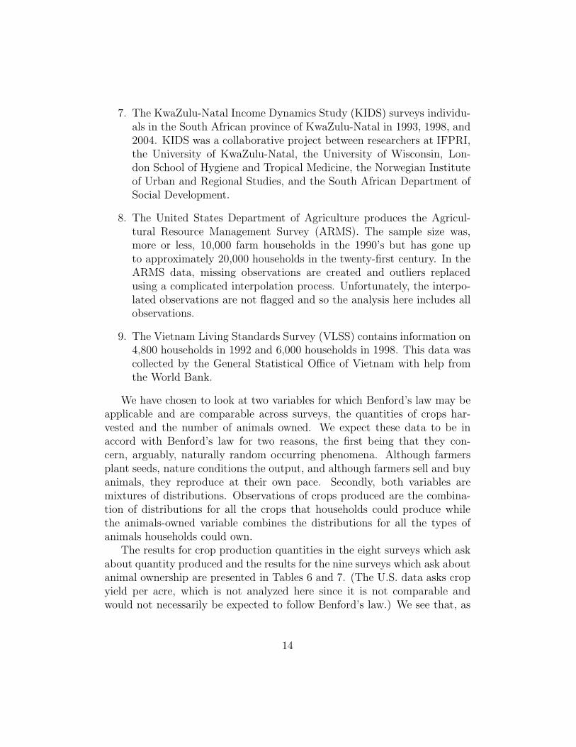
7. The KwaZulu-Natal Income Dynamics Study (KIDS) surveys individu-als in the South African province of KwaZulu-Natal in 1993, 1998, and2004. KIDS was a collaborative project between researchers at IFPRI,the University of KwaZulu-Natal, the University of Wisconsin, Lon-don School of Hygiene and Tropical Medicine, the Norwegian Instituteof Urban and Regional Studies, and the South African Department ofSocial Development.

8. The United States Department of Agriculture produces the Agricul-tural Resource Management Survey (ARMS). The sample size was,more or less, 10,000 farm households in the 1990’s but has gone upto approximately 20,000 households in the twenty-first century. In theARMS data, missing observations are created and outliers replacedusing a complicated interpolation process. Unfortunately, the interpo-lated observations are not flagged and so the analysis here includes allobservations.

9. The Vietnam Living Standards Survey (VLSS) contains information on4,800 households in 1992 and 6,000 households in 1998. This data wascollected by the General Statistical Office of Vietnam with help fromthe World Bank.

We have chosen to look at two variables for which Benford’s law may beapplicable and are comparable across surveys, the quantities of crops har-vested and the number of animals owned. We expect these data to be inaccord with Benford’s law for two reasons, the first being that they con-cern, arguably, naturally random occurring phenomena. Although farmersplant seeds, nature conditions the output, and although farmers sell and buyanimals, they reproduce at their own pace. Secondly, both variables aremixtures of distributions. Observations of crops produced are the combina-tion of distributions for all the crops that households could produce whilethe animals-owned variable combines the distributions for all the types ofanimals households could own.

The results for crop production quantities in the eight surveys which askabout quantity produced and the results for the nine surveys which ask aboutanimal ownership are presented in Tables 6 and 7. (The U.S. data asks cropyield per acre, which is not analyzed here since it is not comparable andwould not necessarily be expected to follow Benford’s law.) We see that, as

14

expected, the two tests (the χ2 statistic and V ∗N test) tend to rise with sample

size, while the distance measures of r, m, d∗, and a∗ do not.The data from Bangladesh, Ghana, Paraguay, and the United States

are consistently relatively close to Benford’s law; the data from Mexico andPakistan seem to be the least in accord with Benford’s law; and the datafrom Peru, South Africa, and Vietnam are somewhere in the middle.10 Thedata from Mexico and Pakistan are the only ones with correlations below.90 and m and d∗ statistics higher than 0.10 for both animals owned andcrops produced. Comparing the χ2 and V ∗

N from Mexico with those of othersurveys of comparable sizes such as Vietnam, Peru in 1985, and Bangladeshwe find that the test statistics for the data from Mexico are much higherthan those in the other three data sets. The test statistics for the Pakistandata are more in line with those of the other smaller data sets.

Comparing the quality of data on crop production (a component of in-come) with that on animals owned (a component of wealth), neither seemsto be clearly better in all of the data sets. Crops are more in accord withBenford than animals in the data sets from Pakistan and Vietnam while theopposite is true in the data from Mexico and South Africa. In the other datasets the two types of variables perform equally well.

The data from the United States performs extremely well in comparisonwith the data sets from developing countries. This could be because farm-ers in the U.S. tend to consult their records while answering surveys andso their answers involve less guesstimation and are more ‘correct’ than thecorresponding answers given by farmers in developing countries. It couldalso be due to the fact that missing values and outliers in the U.S. dataset are replaced with interpolated values. Since the National AgriculturalStatistics Service (NASS) does not flag interpolated values, it is impossibleto distinguish between these two hypotheses.

10We asked Markus Goldstein why he thought the data collected in Ghana was of suchhigh quality. Markus replied that, as do many other organizations, they paid enumeratorshigh wages so they would be afraid of losing their jobs. More unusually, they made a pointof hiring almost all high school graduates, with only one college graduate. Lastly, Chrisand Markus sat in on interviews for an average of one and a half days a week.

15

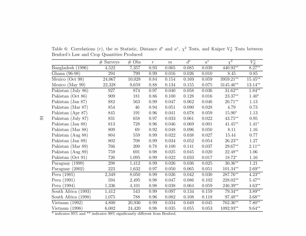
Table 6: Correlations (r), the m Statistic, Distance d∗ and a∗, χ2 Tests, and Kuiper V ∗N Tests between

Benford’s Law and Crop Quantities Produced

# Surveys # Obs r m d∗ a∗ χ2 V ∗N

Bangladesh (1996) 4,522 7,357 0.93 0.065 0.085 0.039 440.92∗∗ 8.27∗∗

Ghana (96-98) 294 799 0.99 0.016 0.026 0.010 8.45 0.85Mexico (Oct 98) 24,067 10,028 0.84 0.154 0.169 0.059 3959.21∗∗ 15.45∗∗

Mexico (May 99) 22,328 9,659 0.88 0.134 0.155 0.075 3145.46∗∗ 13.14∗∗

Pakistan (July 86) 927 874 0.97 0.040 0.058 0.036 31.62∗∗ 1.84∗∗

Pakistan (Oct 86) 909 181 0.86 0.100 0.128 0.016 23.37∗∗ 1.40∗

Pakistan (Jan 87) 882 563 0.99 0.047 0.062 0.046 20.71∗∗ 1.13Pakistan (Mar 87) 854 46 0.94 0.051 0.090 0.028 4.79 0.73Pakistan (Apr 87) 845 191 0.96 0.041 0.078 0.059 15.90∗ 1.13Pakistan (July 87) 831 658 0.97 0.033 0.061 0.022 43.75∗∗ 0.95Pakistan (Jan 88) 813 728 0.96 0.046 0.069 0.001 41.45∗∗ 1.41∗

Pakistan (Mar 88) 809 69 0.92 0.048 0.096 0.050 8.11 1.16Pakistan (Aug 88) 804 559 0.99 0.022 0.038 0.027 15.44 0.77Pakistan (Jan 89) 802 708 0.99 0.034 0.052 0.054 26.23∗∗ 1.27Pakistan (Mar 89) 766 200 0.78 0.100 0.141 0.037 29.67∗∗ 2.11∗∗

Pakistan (Aug 89) 759 691 0.98 0.025 0.045 0.020 22.48∗∗ 1.06Pakistan (Oct 91) 726 1,095 0.99 0.022 0.033 0.017 18.72∗ 1.16Paraguay (1999) 298 1,412 0.99 0.026 0.036 0.025 30.36∗∗ 1.21Paraguay (2002) 223 1,632 0.97 0.050 0.065 0.051 101.34∗∗ 2.69∗∗

Peru (1985) 2,349 8,050 0.99 0.026 0.042 0.030 287.76∗∗ 4.23∗∗

Peru (1991) 594 2,495 0.98 0.047 0.086 0.102 228.02∗∗ 5.47∗∗

Peru (1994) 1,336 4,101 0.98 0.038 0.064 0.059 246.39∗∗ 4.63∗∗

South Africa (1993) 1,412 543 0.99 0.097 0.134 0.159 79.34∗∗ 3.89∗∗

South Africa (1998) 1,075 788 0.96 0.082 0.108 0.118 97.48∗∗ 3.68∗∗

Vietnam (1992) 4,800 20,936 0.99 0.034 0.049 0.045 762.36∗∗ 7.80∗∗

Vietnam (1998) 6,002 24,420 0.98 0.035 0.055 0.053 1092.93∗∗ 9.64∗∗


16

Table 7: Correlations (r), the m Statistic, Distance d∗ and a∗, χ2 Tests, and Kuiper V ∗N Tests between

Benford’s Law and Animals Owned# Surveys # Obs r m d∗ a∗ χ2 V ∗

N

Bangladesh (1996) 4,522 6,807 0.99 0.057 0.073 0.078 333.56∗∗ 7.25∗∗

Ghana (Nov 96) 294 332 0.98 0.023 0.042 0.013 7.79 0.79Ghana (Dec 97) 294 335 0.99 0.016 0.028 0.006 2.76 0.60Ghana (Aug 98) 294 306 0.99 0.017 0.033 0.007 3.83 0.75

Mexico (Nov 97) 24,077 48,042 0.99 0.021 0.044 0.007 1142.88∗∗ 6.64∗∗

Mexico (Oct 98) 24,067 37,130 1.00 0.098 0.119 0.138 4052.83∗∗ 27.23∗∗

Mexico (May 99) 22,328 34,539 1.00 0.108 0.127 0.142 4065.22∗∗ 28.15∗∗

Mexico (Nov 99) 23,266 38,817 0.99 0.114 0.133 0.141 4750.71∗∗ 30.85∗∗

Mexico (May 00) 22,627 37,580 1.00 0.115 0.133 0.146 4703.09∗∗ 29.88∗∗

Pakistan (July 86) 927 1,562 0.96 0.119 0.155 0.183 358.08∗∗ 8.07∗∗

Pakistan (Oct 86) 909 1,981 0.94 0.120 0.141 0.153 386.43∗∗ 7.36∗∗

Pakistan (Jan 87) 882 2,010 0.77 0.128 0.171 0.061 395.04∗∗ 8.82∗∗

Pakistan (July 87) 831 1,961 0.84 0.116 0.147 0.078 326.96∗∗ 7.95∗∗

Pakistan (Mar 88) 809 1,786 0.77 0.171 0.193 0.095 456.86∗∗ 8.58∗∗

Pakistan (Mar 89) 766 1,838 0.81 0.154 0.174 0.092 402.10∗∗ 8.28∗∗

Pakistan (Oct 91) 726 559 0.71 0.135 0.158 0.067 89.93∗∗ 3.83∗∗

Paraguay (1999) 298 827 0.93 0.061 0.087 0.043 56.21∗∗ 3.09∗∗

Paraguay (2002) 223 676 0.99 0.044 0.056 0.042 18.52∗ 1.14

Peru (1985) 2,349 8,007 0.98 0.072 0.089 0.092 696.76∗∗ 8.73∗∗

Peru (1991) 594 2,369 0.97 0.069 0.090 0.104 220.62∗∗ 4.82∗∗

Peru (1994) 1,336 3,392 0.99 0.048 0.059 0.064 126.40∗∗ 3.72∗∗

South Africa (1993) 1,412 696 1.00 0.019 0.027 0.010 4.35 0.52South Africa (1998) 1,075 694 1.00 0.039 0.045 0.042 11.26 1.18

United States (1996) 9,573 8,549 1.00 0.009 0.016 0.002 33.29∗∗ 1.81∗∗

United States (1997) 11,724 20,345 1.00 0.016 0.025 0.031 188.41∗∗ 4.40∗∗

United States (1998) 11,812 11,127 1.00 0.013 0.021 0.020 56.90∗∗ 2.12∗∗

United States (1999) 10,251 8,749 1.00 0.011 0.017 0.021 36.58∗∗ 1.77∗∗

United States (2000) 10,309 8,944 1.00 0.008 0.014 0.013 26.00∗∗ 1.69∗∗

United States (2001) 7,699 6,651 0.99 0.018 0.025 0.012 41.85∗∗ 2.46∗∗

United States (2002) 12,391 16,257 1.00 0.012 0.017 0.019 85.63∗∗ 2.84∗∗

United States (2003) 18,459 14,066 1.00 0.014 0.021 0.027 99.90∗∗ 3.25∗∗

United States (2004) 20,579 15,798 1.00 0.009 0.011 0.008 22.54∗∗ 1.11United States (2005) 22,843 17,228 1.00 0.019 0.017 0.005 56.06∗∗ 2.66∗∗

Vietnam (1992) 4,800 8,005 0.99 0.102 0.148 0.171 1372.73∗∗ 16.79∗∗

Vietnam (1998) 6,002 8,351 0.97 0.092 0.120 0.142 1154.57∗∗ 13.95∗∗


17

Note that the November 1997 round of data from Mexico appears to beof much higher quality than the later rounds.This is interesting because thefirst round of the Mexican Progresa data, the Encaseh, was a census usedfor targeting the households. This collected only the most easily collectableinformation and lasted only fifteen to twenty minutes. The later surveys,the Encels, were classic household surveys collecting detailed informationon consumption, labor, health, income, and more. These surveys lastedone to two hours. These results suggest that longer surveys may tire outenumerators and/or respondents and can have a serious effect on data quality.

3.1 Male vs Female Respondents

Five of the surveys identify which household member responded to the ques-tionnaire. If women in developing countries are in charge of livestock whilemen are in charge of crop production, one might think that women can answerquestions about livestock more accurately, while men can answer questionsabout crop production more accurately. On the other hand, this ignores thefact that households endogenously chose which household member answersthe survey questions. In Tables 8 and 9 we test this idea.

The test results are always much higher for males than females, but thatis due to the higher sample size of male respondents. The four distancemeasures, on the other hand, are quite similar for males and females inthe developing country data. These results suggest that there is not muchof a difference in the overall quality of information given by male versusfemale respondents in developing countries. On the other hand, in the USdata, according to the distance measures female respondents consistently givedata less in accord with Benford’s law. Perhaps women in the US are lessinvolved with agriculture than are women in developing countries and so giveless-well informed answers. Women in the US also give a much higher shareof answers starting with the first digit of five than do men or women in othercountries. Additionally, males and females do not seem to perform differentlyin answering questions related to crops versus livestock. We might interpretthese results as showing that enumerators can get reasonable quality datafrom both male and female household members.

18

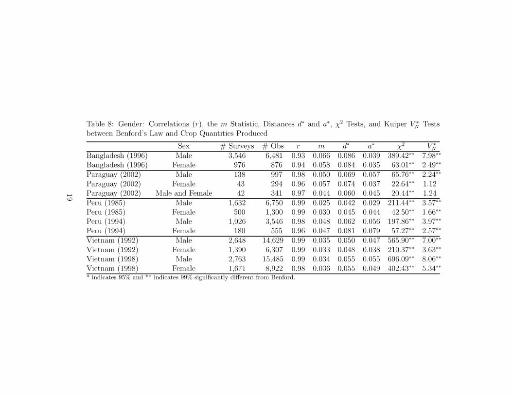
Table 8: Gender: Correlations (r), the m Statistic, Distances d∗ and a∗, χ2 Tests, and Kuiper V ∗N Tests

between Benford’s Law and Crop Quantities Produced

Sex # Surveys # Obs r m d∗ a∗ χ2 V ∗N

Bangladesh (1996) Male 3,546 6,481 0.93 0.066 0.086 0.039 389.42∗∗ 7.98∗∗

Bangladesh (1996) Female 976 876 0.94 0.058 0.084 0.035 63.01∗∗ 2.49∗∗

Paraguay (2002) Male 138 997 0.98 0.050 0.069 0.057 65.76∗∗ 2.24∗∗

Paraguay (2002) Female 43 294 0.96 0.057 0.074 0.037 22.64∗∗ 1.12Paraguay (2002) Male and Female 42 341 0.97 0.044 0.060 0.045 20.44∗∗ 1.24Peru (1985) Male 1,632 6,750 0.99 0.025 0.042 0.029 211.44∗∗ 3.57∗∗

Peru (1985) Female 500 1,300 0.99 0.030 0.045 0.044 42.50∗∗ 1.66∗∗

Peru (1994) Male 1,026 3,546 0.98 0.048 0.062 0.056 197.86∗∗ 3.97∗∗

Peru (1994) Female 180 555 0.96 0.047 0.081 0.079 57.27∗∗ 2.57∗∗

Vietnam (1992) Male 2,648 14,629 0.99 0.035 0.050 0.047 565.90∗∗ 7.00∗∗

Vietnam (1992) Female 1,390 6,307 0.99 0.033 0.048 0.038 210.37∗∗ 3.63∗∗

Vietnam (1998) Male 2,763 15,485 0.99 0.034 0.055 0.055 696.09∗∗ 8.06∗∗

Vietnam (1998) Female 1,671 8,922 0.98 0.036 0.055 0.049 402.43∗∗ 5.34∗∗


19

Table 9: Gender: Correlations (r), the m Statistic, Distance d∗ and a∗, χ2 Tests, and Kuiper V ∗N Tests

between Benford’s Law and Animals Owned

Sex # Surveys # Obs r m d∗ a∗ χ2 V ∗N

Bangladesh (1996) Male 3,546 5,657 0.98 0.059 0.073 0.077 281.84∗∗ 6.34∗∗

Bangladesh (1996) Female 976 1,150 0.99 0.056 0.083 0.082 59.64∗∗ 3.60∗∗

Paraguay (2002) Male 138 414 0.99 0.069 0.078 0.066 17.77∗ 1.41∗

Paraguay (2002) Female 43 126 0.96 0.056 0.062 0.000 6.60 0.64Paraguay (2002) Male and Female 42 136 0.95 0.065 0.078 0.012 12.63 0.87

Peru (1985) Male 1,632 6,422 0.97 0.078 0.094 0.102 563.81∗∗ 8.28∗∗

Peru (1985) Female 500 1,585 0.99 0.048 0.076 0.097 99.77∗∗ 3.55∗∗

Peru (1994) Male 1,026 2,915 0.99 0.048 0.059 0.061 105.57∗∗ 3.48∗∗

Peru (1994) Female 180 477 0.98 0.048 0.068 0.081 28.85∗∗ 1.88∗∗

United States (1996) Male 8,721 7,870 1.00 0.010 0.016 0.001 31.29∗∗ 1.88∗∗

United States (1996) Female 422 396 0.98 0.029 0.047 0.015 9.61 0.85United States (1997) Male 11,290 19,642 1.00 0.016 0.025 0.030 179.81∗∗ 4.29∗∗







United States (2003) Female 873 687 0.98 0.030 0.049 0.003 18.68∗ 1.62∗∗

United States (2004) Male 19,458 14,980 1.00 0.009 0.011 0.009 22.05∗∗ 1.08United States (2004) Female 1,121 818 1.00 0.017 0.024 0.010 5.01 0.69United States (2005) Male 21,694 16,395 1.00 0.009 0.017 0.006 54.59∗∗ 2.59∗∗

United States (2005) Female 1,149 833 0.99 0.031 0.037 0.017 12.15 0.96

Vietnam (1992) Male 2,648 5,536 0.99 0.100 0.144 0.169 913.25∗∗ 13.57∗∗

Vietnam (1992) Female 1,390 2,469 0.99 0.107 0.156 0.176 464.11∗∗ 9.93∗∗

Vietnam (1998) Male 2,763 5,338 0.97 0.090 0.115 0.136 669.87∗∗ 10.94∗∗

Vietnam (1998) Female 1,671 3,009 0.98 0.095 0.131 0.152 443.34∗∗ 9.00∗∗


20

3.2 Enumerators’ Opinions and Data Fabrication

The survey from Bangladesh asked enumerators to judge both the accuracyof the respondents’ answers as well as the seriousness and attentiveness ofthe respondent. Possible answers were: excellent, good, fair, not so bad, andvery bad. In Table 10 we compare those surveys which were judged to be fair,not so bad, or very bad in terms of either accuracy or attentiveness (or both)with those that were good or excellent in both categories. As there are manymore ‘good’ observations than ‘bad’, the test statistics for the good data arehigher. More suggestively, the correlation with Benford is also higher in the‘bad’ data while the m, d∗, and a∗ distance measures are lower. If anything,the bad data seems to be better than the good data! Although this analysisis only applied to one data set, it suggests that enumerator evaluations ofthe respondents’ data should be taken with a grain of salt.

When carrying out field work in May 2001 researchers working on theKIDS South Africa data found evidence that some of the 1998 householdswere fabricated by the enumerators. In 2004 it was concluded that onlysix clusters of data might have been fabricated and these have been removedfrom the version of the data available to the public. We have gained access tothese deleted clusters and compare the data from those households to thosein the rest of the survey. While only some of the households in the clustermay have been found to have been fabricated, all of them were dropped fromthe data set to be conservative.

Again, it is quite difficult to make comparisons due to the small numberof observations in the clusters categorized as potentially being fabricated.Still, for the animal data, the ‘fabricated’ data performs much worse thanthe non-fabricated data according to all measures and tests. The resultsfor the crop production data are less stark but are still suggestive of thelow quality of data collected in the clusters in which the households werepotentially fabricated.

It is interesting to note that data which enumerators qualify as ‘good’is actually less in accord with Benford’s law, as is data that enumeratorsfabricate. Perhaps this is due to enumerators’ mistaken perception as towhat realistic data ought to look like.

21

Table 10: Enumerator Opinion and Data Fabrication: Correlations (r), the m Statistic, Distance d∗ and a∗,χ2 Tests, and Kuiper V ∗

N Tests between Benford’s Law and Animals Owned and Crop Quantities Produced

Quality # Surveys # Obs r m d∗ a∗ χ2 V ∗N

Crops ProducedBangladesh (1996) ‘Bad’ 1,384 2,096 0.95 0.052 0.070 0.029 94.33∗∗ 3.46∗∗

Bangladesh (1996) ‘Good’ 3,107 5,204 0.92 0.070 0.093 0.042 360.55∗∗ 7.53∗∗

Animals OwnedBangladesh (1996) ‘Bad’ 1,384 2,053 1.00 0.046 0.068 0.074 80.56∗∗ 3.84∗∗

Bangladesh (1996) ‘Good’ 3,107 4,716 0.98 0.066 0.078 0.079 262.15∗∗ 6.16∗∗

Crops ProducedSouth Africa ‘Fabricated’ 283 62 0.99 0.118 0.163 0.204 14.60∗ 1.78∗∗

South Africa ‘Not Fabricated’ 2,487 1,331 0.98 0.076 0.113 0.134 167.20∗∗ 5.22∗∗

Animals OwnedSouth Africa ‘Fabricated’ 283 50 0.70 0.156 0.253 0.061 29.87∗∗ 1.90∗∗

South Africa ‘Not Fabricated’ 2,487 1,390 1.00 0.029 0.033 0.026 12.54 1.09* indicates 95% and ** indicates 99% significantly different from Benford.

22

4 Implications for Theory and Practice

When respondents are asked for answers of which they are unsure they tendto estimate and round to ‘nice’ numbers. In addition, at least in this study,larger data sets collected by government statistical offices seem to be of lowerquality than data collected by academic researchers. The Progresa data inMexico and the IFPRI data from Pakistan are particularly inconsistent withBenford’s law. These are issues which should not be ignored. Althoughsophisticated econometric techniques are available to deal with measurementerror once it is identified, we should be much more careful and serious aboutboth enumerator quality and designing questionnaires that elicit data withminimal respondent errors.

We have shown evidence that suggests data errors increase for more-diversified farmers. If certain questions are more prone to errors than others,then we will find that surveys for households which are more active in thoseareas will contain more errors, which can cause serious problems if the datais used in an estimation and inference context. We have also shown thatthere are certain questions which are more or less susceptible to responseerrors. Questions for which people tend to be unsure of the answer or forwhich people may have an incentive to answer dishonestly, such as donationsto church or production of secondary crops, are more susceptible to errors.

Although the exact questions which lead to departures from Benford’sFSD distribution may be different in each country and situation, Benford’slaw provides a simple means of testing for such irregularities in data. Re-searchers can easily and quickly test whether the variable that is of mostinterest to their research follows Benford’s law or exhibits errors. They canalso test whether certain enumerators are collecting more irregular data, andwhether households in certain clusters appear more irregular. The data whichis presumed to be fabricated in the South African KIDS data was only noticedwhen researchers tried to go back to resurvey those households. Benford’slaw could be used for a similar purpose, especially in cross-sectional data.

Glewwe & Dang (2005) show how having computers available for data-input at the district level, so that mistakes can be found more quickly andhouseholds reinterviewed sooner, can improve data quality. These computerscould easily be programmed to include a Benford’s law component to test forthe quality of responses to different questions and from different enumerators.

These results demonstrate why one should not consider only Benford’slaw when evaluating enumerators or data sets. For example, while the data

23

collected in 1999 on crop quantities produced are much more in accord withBenford’s law than that collected in 2002, the evidence suggests that thisis not because the enumerators were better in 1999. The enumerators in1999 seem to have only collected data on the most important crops, whilethe enumerators in 2002 collected data on many more crops, but for whichthere was more respondent error. Hence, while Benford’s law suggests thatthe 1999 data contains less measurement error, other evidence suggests thatthis is because the 1999 data includes fewer crops. This is a warning againstusing Benford’s law in isolation when judging the quality of a data set.

5 Conclusions

We have demonstrated how Benford’s law can be used to detect data ab-normalities arising both from questions that are difficult to answer and fromenumerator errors. While econometricians and applied economists spendmuch energy correcting for measurement error in pre-existing data sets, theyshould also try to avoid it by detecting these problems early in the data-collection process.

There remains much room for future research on topics related to surveydesign and enumerator contracts. Can researchers articulate which typesof questions and situations will lead to more accurate answers in general?For example, the following situations may affect error: use of interpreters,presence of non-family members during the interview, participation of morethan one family member in the interview, and participation of female ratherthan male household members.

Furthermore, while Philipson & Malani (1999) show how random enu-merator audits with prizes for accurate reporting can be used to decreaseerrors when direct data verification is possible, a contract has not yet beendesigned for data tests such as Benford’s law which may be more prone toboth Type I and Type II errors. These are important steps that should betaken to increase the quality of data production in addition to that of dataconsumption.

Finally, Scott & Fasli (2001) note that even in Benford’s original paperonly half of the data sets provide a reasonably close fit with Benford’s law.Consequently, it seems possible that a family of data-based FSD distributionsmay be more compatible with observed data sets than Benford’s distributionitself. To this end, Grendar et al. (2007) use information-theoretic methods to

24

develop a family of alternative Benford-like distributions. As these methodsare refined, new tests of data quality may arise that provide insights onBenford’s law and other scale invariant natural phenomenon. As a side note,our ongoing research using insights from this research concerning survey datahas turned to the use of Benford’s FSD to identify falsification in clinical trials(a life and death matter) and manipulation and collusion in market data.

References

Benford, F. (1938), ‘The law of anomalous numbers’, Proceedings of the

American Philosophical Society 78(4), 551–572.

Berger, A. & Hill, T. P. (2007), ‘Newton’s method obeys Benford’s law’,American Mathematical Monthly 114(7), 588–601.

Biemer, P. P., Groves, R. M., Lyberg, L. E., Mathiowetz, N. A. & Sudman,S., eds (1991), Measurement Errors in Surveys, New York: John Wiley &Sons.

Carslaw, C. A. P. N. (1988), ‘Anomalies in income numbers: Evidence ofgoal oriented behavior’, Accounting Review 63(2), 321–327.

Cho, W. K. T. & Gaines, B. J. (2007), ‘Breaking the (Benford) law: Sta-tistical fraud detection in campaign finance’, The American Statistician

61(3), 1–6.

de Marchi, S. & Hamilton, J. T. (2006), ‘Assessing the accuracy of self-reported data: An evaluation of the toxics release inventory’, Journal of

Risk and Uncertainty 32(1), 57–76.

Diaconis, P. (1977), ‘The distribution of leading digits and uniform distribu-tion mod 1’, The Annals of Probability 5(1), 72–81.

Durtschi, C., Hillison, W. & Pacini, C. (2004), ‘The effective use of Benford’slaw to assist in detecting fraud in accounting data’, Journal of Forensic

Accounting 5(1), 17–34.

Geyer, C. L. & Williamson, P. P. (2004), ‘Detecting fraud in data sets usingBenford’s law’, Computation in Statistics: Simulation and Computation

33(1), 229–246.

25

Giles, D. E. (2007), ‘Benford’s law and naturally occurring prices in certainebaY auctions’, Applied Economics Letters 14(3), 157–161.

Glewwe, P. & Dang, H.-A. H. (2005), The impact of decentralized data entryon the quality of household survey data in developing countries: Evidencefrom a randomized experiment in Vietnam. Unpublished Manuscript.

Grendar, M., Judge, G. & Schechter, L. (2007), ‘An empirical non-parametriclikelihood family of data-based Benford-like distributions’, Physica A: Sta-

tistical Mechanics and its Applications 380, 429–438.

Grosh, M. & Glewwe, P., eds (2000), Designing Household Survey Ques-

tionnaires for Developing Countries: Lessons from 15 years of the Living

Standards Measurement Study, Washington DC: The World Bank.

Groves, R. M. (1989), Survey Errors and Survey Costs, New York: JohnWiley & Sons.

Hill, T. P. (1995), ‘A statistical derivation of the significant-digit law’, Sta-

tistical Science 10(4), 354–363.

Hill, T. P. & Schurger, K. (2005), ‘Regularity of digits and significantdigits of random variables’, Stochastic Processes and Their Applications

115(10), 1723–1743.

Leemis, L. M., Schmeiser, B. W. & Evans, D. L. (2000), ‘Survival distribu-tions satisfying Benford’s law’, The American Statistician 54(4), 236–241.

Livio, M. (2002), The Golden Ratio: The Story of Phi, the World’s Most

Astonishing Number, New York: Broadway.

Morrow, J. (2007), Benford’s law, families of distributions, and a test basis.Unpublished Manuscript.

Newcomb, S. (1881), ‘Note on the frequency of use of the different digits innatural numbers’, American Journal of Mathematics 4(1), 39–40.

Nigrini, M. J. (1996), ‘A taxpayer compliance application of Benford’s law’,Journal of the American Taxation Association 18(1), 72–91.

26

Nye, J. & Moul, C. (2007), ‘The political economy of numbers: On theapplication of Benford’s law to international macroeconomic statistics’,The B.E. Journal of Macroeconomics 7(1 (Topics)).

Philipson, T. & Malani, A. (1999), ‘Measurement errors: A principalinvestigator-agent approach’, Journal of Econometrics 91(2), 273–298.

Pietronero, L., Tosatti, E., Tosatti, V. & Vespignani, A. (2001), ‘Explainingthe uneven distribution of numbers in nature: The laws of Benford andZipf’, Physica A: Statistical Methods and its Applications 293(1-2), 297–304.

Raimi, R. (1976), ‘The first digit problem’, American Mathematical Monthly

83(7), 521–538.

Rodriguez, R. J. (2004), ‘First significant digit patterns from mixtures ofuniform distributions’, The American Statistician 58(1), 64–71.

Schatte, P. (1988), ‘On mantissa distributions in computing and Benford’slaw’, Journal of Information Processing and Cybernetics 24(10), 443–455.

Scott, P. D. & Fasli, M. (2001), Benford’s law: An empirical investigationand a novel explanation. Unpublished Manuscript.

Stephens, M. A. (1970), ‘Use of the Kolmogorov-Smirnov, Cramer-Von Misesand related statistics without extensive tables’, Journal of the Royal Sta-

tistical Society, Series B 32(1), 115–122.

Sudman, S., Bradburn, N. M. & Schwarz, N. (1996), Thinking About An-

swers, San Franciscco: Jossey-Bass Publishers.

Varian, H. (1972), ‘Benford’s law’, The American Statistician 26(3), 65.

A Appendix: http://www.checkyourdata.com

A website is available with an online utility into which you can easily inputvariables from any data set (as a comma separated value (csv) file) and see ifyour data is in accord with Benford’s law. At http://www.checkyourdata.com,

27

there is a tutorial explaining how to get data from Stata into the online util-ity and a video tutorial on the basics of using the utility. In addition, in theonline utility itself, there is a help tab which gives more detailed informationon the available commands.

When using the utility, researchers can either use the pull-down tab com-mands or can type commands directly into the command window. Afterinputting data, all of the tests and measures discussed in this paper are cal-culated. It is also possible to combine multiple variables, for example to lookat corn, soy, wheat, and cotton production variables together. One can splitvariables as well, for example to look at data collected from male and femalerespondents separately, or by different enumerators separately. The programalso can make graphs of the data and gives other summary statistics.

B Appendix: Extra Tables and Figures

Table B-1: Summary Statistics for 2002 Paraguay Data

Household VariablesVariable Mean (Std. Dev.)Theft Experienced 111,000 (336,000)Gifts Given 306,000 (524,000)Annual Income 28,300,000 (72,100,000)Median Annual Income 9,046,000Family Size 5.6 (2.4)Land Owned (hectares) 36.6 (95.8)

Respondent VariablesVariable Mean (Std. Dev.)Male 79%Age 52.2 (14.8)Years of Education 4.9 (2.7)Obs 223The relevant exchange rate is approximately 4,800 Guaranies to the dollar.

28

Table B-2: Correlations (r), the m Statistic, Distances d∗ and a∗, χ2 Tests,and Kuiper V ∗

N Tests between Benford’s Law and Animals Owned in 1999and 2002

Surveys Obs r m d∗ a∗ χ2 V ∗N

Total in 1999 298 827 0.93 0.061 0.087 0.043 56.21∗∗ 3.09∗∗

Enumerator 1 33 105 0.94 0.081 0.098 0.076 10.73 0.88Enumerator 2 36 103 0.97 0.050 0.078 0.086 8.18 1.09Enumerator 3 33 91 0.83 0.079 0.125 0.010 14.87 1.39∗

Enumerator 4 37 94 0.78 0.099 0.152 0.027 16.24∗ 1.80∗∗

Enumerator 5 27 78 0.90 0.068 0.109 0.065 9.35 1.13Enumerator 6 8 29 0.86 0.071 0.121 0.026 6.43 0.61Enumerator 7 32 93 0.96 0.039 0.062 0.016 4.85 0.60Enumerator 8 10 31 0.93 0.147 0.184 0.178 9.15 1.37∗

Enumerator 9 32 84 0.82 0.098 0.143 0.036 14.86 1.33∗

Enumerator 10 22 50 0.61 0.184 0.246 0.047 20.44∗∗ 1.76∗∗

Total in 2002 223 676 0.99 0.044 0.056 0.042 18.52∗ 1.14Enumerator 1 71 211 0.97 0.030 0.058 0.006 7.58 0.83Enumerator 2 75 223 0.96 0.051 0.083 0.034 15.81∗ 0.77Enumerator 3 77 242 0.99 0.063 0.078 0.082 11.77 1.34∗


29

Table B-3: Correlations (r), the m Statistic, Distances d∗ and a∗, χ2 Tests,and Kuiper V ∗

N Tests between Benford’s Law and Quantities Produced

Surveys Obs Obs/Survey r m d∗ a∗ χ2 V ∗N

Total in 1999 298 1412 4.7 0.99 0.026 0.036 0.025 30.36∗∗ 1.21Enumerator 1 33 159 4.8 0.90 0.065 0.098 0.023 20.80∗∗ 1.57∗

Enumerator 2 36 139 3.9 0.98 0.033 0.064 0.057 6.40 0.85Enumerator 3 33 153 4.6 0.97 0.087 0.052 0.074 13.61 1.23Enumerator 4 37 162 4.4 0.97 0.048 0.064 0.051 6.84 0.71Enumerator 5 27 136 5.0 0.98 0.052 0.083 0.087 11.12 1.06Enumerator 6 8 43 5.4 0.78 0.084 0.144 0.084 9.21 0.71Enumerator 7 32 149 4.7 0.96 0.095 0.112 0.042 12.15 1.42∗

Enumerator 8 10 60 6.0 0.96 0.049 0.090 0.052 7.03 0.44Enumerator 9 32 202 6.3 0.95 0.043 0.076 0.045 14.33 1.47∗

Enumerator 10 22 89 4.0 0.96 0.055 0.069 0.045 5.55 0.78

Total in 2002 223 1632 7.3 0.97 0.050 0.065 0.051 101.34∗∗ 2.69∗∗

Enumerator 1 71 516 7.3 0.97 0.031 0.057 0.042 28.20∗∗ 1.50∗

Enumerator 2 75 556 7.4 0.98 0.049 0.070 0.061 37.58∗∗ 1.68∗∗

Enumerator 3 77 560 7.3 0.94 0.073 0.092 0.050 67.92∗∗ 1.97∗∗

*-95% and **-99% significantly different from Benford.

30

detecting problems in survey data using benford’s · pdf filedetecting problems in...

Documents