detection of cardiac troponin i in circulation using raman...
TRANSCRIPT

Detection of Cardiac Troponin I in circulation using Raman Spectroscopy;
An Approach to Prediction of Myocardial Infarction
by Amir Pasha Tashakor
B.Sc. (Hons.), Simon Fraser University, 2010
Thesis Submitted in Partial Fulfillment of the Requirements for the Degree of
Master of Applied Sciences
in the School of Engineering Science
Faculty of Applied Sciences
Amir Pasha Tashakor 2012
SIMON FRASER UNIVERSITY Spring 2012
All rights reserved. However, in accordance with the Copyright Act of Canada, this work may
be reproduced, without authorization, under the conditions for “Fair Dealing.” Therefore, limited reproduction of this work for the
purposes of private study, research, criticism, review and news reporting is likely to be in accordance with the law, particularly if cited appropriately.

ii
Approval
Name: Pasha Tashakor Degree: Master of Applied Science Title of Thesis: Detection of Cardiac Troponin I in Circulation Using
Raman Spectroscopy; An Approach to Prediction of Myocardial Infarction
Examining Committee: Chair: Dr. Parvaneh Saeedi, P.Eng., Assistant Professor
Dr. Andrew Rawicz, P. Eng. Senior Supervisor Professor, School of Engineering Science
Dr. Glen Tibbits Supervisor Professor and chair, Department of Biomedical Physiology and Kinesiology
Mr. Bruno Jaggi, P. Eng. External Examiner Adjunct Professor, Department of Biomedical Engineering, University of British Columbia
Date Defended/Approved: April 2, 2012

iii
Partial Copyright Licence

iv
Abstract
Myocardial infarction (MI) pertains to cardiac tissue death, secondary to
prolonged inadequate perfusion to myocardial cells. Despite medical advances, MI
remains a global leading cause of mortality and morbidity. Minute and subclinical
physiological changes occur hours prior to a symptomatically appreciable ‘attack’. These
well-established phenomena involve the release of specific cardiac biomarkers into
systemic circulation. Quantitative measurement of systemic cTnI concentrations is
widely and routinely implemented in the diagnosis of MI. However, current technology
is limited to detection of ‘post-attack’ concentrations, which often indicates irreversible
damage. Consequently, we aimed to noninvasively detect concentrations of cTnI
through biophotonic technology. For the first time in literature, we characterized and
repeatedly verified unique Raman signature of mouse cTnI in water and BSA. Further,
we investigated concentration changes, optimized integration durations, and proposed
a conceptual design. This project potentially begets preclinical detection of biomarkers,
earlier diagnosis, prompt medical intervention, and enhanced overall prognosis.
Keywords: Raman Spectroscopy; Cardiac Troponin; Myocardial Infarction; Biophotonics; cTnI

v
Acknowledgements
Foremost, I would like to express my sincere gratitude to my senior supervising
Professor, Andrew Rawicz, whom for the past three years has supported and
encouraged me in my research, my knowledge in engineering as well as other aspects of
life. I would like to thank Professor Glen Tibbits and his research team. This project was
simply impossible without his help and contribution. Further, I would like to thank
Professor Bruno Jaggi who has greatly enriched my knowledge with his exceptional
insights into engineering. I would also like to thank Professor Edward Grant as well as
my senior colleague, Sara Moghaddamjoo, who made this possible with her
unconditional support.
Lastly, I would like to thank my beloved parents for their support and patience. I
am greatly indebted to my brother; this dissertation is simply impossible without him.

vi
Table of Contents
Approval ............................................................................................................................... ii Partial Copyright Licence .................................................................................................... iii Abstract ............................................................................................................................... iv Acknowledgements .............................................................................................................. v Table of Contents ................................................................................................................ vi List of Tables ..................................................................................................................... viii List of Figures ...................................................................................................................... ix List of Acronyms ................................................................................................................. xii Executive Summary ........................................................................................................... xiv
1. Introduction and background information .......................................................... 1 1.1. Introduction ............................................................................................................... 1 1.2. Background ................................................................................................................ 4
1.2.1. Heart Attack ................................................................................................... 4 1.2.2. Mechanism of Troponin release in cytoplasm ............................................... 6 1.2.3. Cardiac Troponin I (cTnI) Measurement ........................................................ 7 1.2.4. Limitations...................................................................................................... 8 1.2.5. Cardiac Troponin T (cTnT) Measurement ...................................................... 9
1.3. Biophotonic Measurement of cTnI .......................................................................... 10 1.4. Florescence Spectroscopy ........................................................................................ 11
1.4.1. Background .................................................................................................. 11 1.4.2. Motivation .................................................................................................... 14 1.4.3. The Experiment ............................................................................................ 14 1.4.4. Florescence Spectroscopy Experiment Results ............................................ 15
1.5. Conclusion ................................................................................................................ 17
2. Cardiac Biomarkers and Biophotonic Measurements ........................................ 19 2.1. Cardiac Biomarkers .................................................................................................. 19
2.1.1. Cardiac Troponin .......................................................................................... 21 2.2. Post Release Modification ....................................................................................... 23 2.3. Literature Review and Discussion ............................................................................ 23
3. Raman Spectroscopy ........................................................................................ 28 3.1. Introduction and Background .................................................................................. 28 3.2. Literature Review ..................................................................................................... 30 3.3. cTnI versus cTnT ....................................................................................................... 31 3.4. Remarks ................................................................................................................... 31
3.4.1. Savitzky-Golay Filter ..................................................................................... 31 3.4.2. Wavelet Transform ...................................................................................... 32

vii
3.5. Spectral Result of Raman Spectroscopy Measurement of cTnI .............................. 32 3.5.1. Signal Processing .......................................................................................... 34 3.5.2. cTnI Raman Signiture for the First Time ...................................................... 36 3.5.3. Results and Discussions ............................................................................... 37
4. Verification of cTnI Signature ............................................................................ 40 4.1. Experiment procedure ............................................................................................. 40 4.2. Verification Result and Discussion ........................................................................... 41
4.2.1. Effect of change in concentration ................................................................ 43 4.2.2. Comparison with Previous Results .............................................................. 44
5. The latest Spectral Result of cTnI in BSA ............................................................ 46 5.1. Results and Discussions ........................................................................................... 46
5.1.1. Effects of Change in integration time .......................................................... 48 5.1.2. Effect of Change in concentration ............................................................... 50 5.1.3. Adjusted cTnI Spectra .................................................................................. 51
5.2. Wavelet Transform .................................................................................................. 53 5.2.1. Effect of Change in integration time ............................................................ 54 5.2.2. Effect of Change in concentration ............................................................... 55 5.2.3. Adjusted cTnI Spectra .................................................................................. 57
5.3. Discussion and Conclusion ....................................................................................... 59
6. Conceptual Design of Raman Detection of cTnI System ..................................... 63 6.1. Literature Review ..................................................................................................... 63 6.2. Conceptual Design of Raman Detection of cTnI System ......................................... 64
7. Conclusion ........................................................................................................ 70
8. References ....................................................................................................... 73
9. Appendix .......................................................................................................... 81 9.1. cTnT .......................................................................................................................... 81 9.2. Florescence Experiment Set Up ............................................................................... 84 9.3. Florescence Spectroscopy ....................................................................................... 86 9.4. cTnI Amino Acid Sequence ...................................................................................... 91 9.5. BSA Amino Acid Sequence ....................................................................................... 92 9.6. BSA Sample Information .......................................................................................... 93 9.7. Sample Codes ........................................................................................................... 94

viii
List of Tables
Table 1: Approximate onset of key events in myocardial infarction. ................................. 5
Table 2: Florescent profile of aromatic amino acids [11] ................................................... 14
Table 3 : Components used to build an optical system .................................................... 15
Table 4: Diagnostic sensitivity and specificity of Troponin I, CK-MB and Total CK [21] ..................................................................................................................... 20
Table 5: The peak values at various concentrations of cTnI ............................................. 87
Table 6: The delta peak values at various molarities of cTnI ............................................ 88
Table 7: Absorption data................................................................................................... 89

ix
List of Figures
Figure 1: Admission Charts of Patients with Suspected Cardiac Damage [6] ...................... 3
Figure 2: Thrombosis in a Coronary Artery [10] ................................................................... 5
Figure 3: The left figure represents a cross section of coronary artery with a 50% occlusion. The right figure shows thrombosis with only three small lumens remaining. [10] .......................................................................................... 6
Figure 4: cTnI enzyme-linked immunosorbent assay (ELISA) test [15] ................................ 8
Figure 5: Principles of florescence [18] ............................................................................... 12
Figure 6: Amino Acid sequence of cTnI (www.pdb.org) [11]. ............................................. 13
Figure 7: Tryptophan chemical structure, showing aromatic rings [19] ............................. 13
Figure 8: Mercury arc lamp expected spectrum [20] ......................................................... 16
Figure 9: Mercury arc lamp spectrum from the spectrometer ........................................ 16
Figure 10: Florescence peak ............................................................................................. 17
Figure 11: Plasma Temporal Profile of Cardiac Diagnostic Markers [22] ........................... 21
Figure 12: Functional Structure of cardiac troponin [23] ................................................... 22
Figure 13: Sequence of events leading to MI based on A. van der Laarse Hypothesis [27] .................................................................................................. 27
Figure 14: Raw cTnI [0.5 mg/mL] in Buffer Sample Raman Spectroscopy ....................... 34
Figure 15: Polyfit subtraction steps for new cTnI. ............................................................ 35
Figure 16: SG Smoothing process for the cTnI .................................................................. 35
Figure 17: First cTnI signature ........................................................................................... 36
Figure 18: New and Old cTnI spectra different concentration ......................................... 38
Figure 19: Water and cTnI sample after noise reduction. ............................................... 41
Figure 20: Different levels of Smoothing of water and sample. ....................................... 42
Figure 21: Snapshot of cTnI sample subtracted from water signal. ................................. 43

x
Figure 22: Effect of change in concentration, adjusted cTnI, 5 seconds integration time .................................................................................................................... 43
Figure 23: cTnI signature. .................................................................................................. 44
Figure 24: Previous results for cTnI signature. ................................................................. 45
Figure 25: Raw samples of BSA [20 g/L] , cTnI(1) [17 g/L] and Water .............................. 47
Figure 26: Change in integration time of cTnI(2) [13 g/L] ................................................ 48
Figure 27: Change in integration time for adjusted cTnI spectra (cTnI(1) [14 g/L]/BSA [3.5 g/L]), (cTnI(1) [12 g/L]/BSA [6 g/L]), (cTnI(1) [10 g/L]/BSA [8 g/L]), (cTnI(2) [10 g/L]/BSA [5 g/L]) ................................................................ 49
Figure 28: Change in concentration of cTnI in water and BSA sample (30 sec. integration time) ................................................................................................ 50
Figure 29: Change in concentration for adjusted cTnI spectra (30 sec. integration time) ................................................................................................................... 51
Figure 30: cTnI signiture zone, Change in integration time for adjusted cTnI spectra (cTnI(1) [10 g/L]/BSA [8 g/L]) ................................................................ 52
Figure 31: FWT Raw samples of BSA [20 g/L] , cTnI(1) [17 g/L] and Water ...................... 53
Figure 32: FWT Change in integration time of cTnI(2) [13 g/L] ........................................ 54
Figure 33: FWT Change in integration time for adjusted cTnI spectra (cTnI(1) [14 g/L]/BSA [3.5 g/L]), (cTnI(1) [12 g/L]/BSA [6 g/L]), (cTnI(1) [10 g/L]/BSA [8 g/L]), (cTnI(2) [10 g/L]/BSA [5 g/L]) ................................................................ 55
Figure 34: FWT Change in concentration of cTnI in water and BSA sample (30 sec. integration time) ................................................................................................ 56
Figure 35: FWT Change in concentration for adjusted cTnI spectra (30 sec. integration time) ................................................................................................ 57
Figure 36: FWT Change in integration time for adjusted cTnI spectra (cTnI(1) [10 g/L]/BSA [8 g/L]) ................................................................................................. 58
Figure 37: cTnI and BSA Raman Peak Analysis .................................................................. 60
Figure 38: cTnI Raman Signature Region .......................................................................... 61
Figure 39: The Tertiary structural model of BSA .............................................................. 62

xi
Figure 40: Patent diagram of Raman Spectrometer for Glucose Measurement form Human Eye [34] ........................................................................................... 64
Figure 41: Anatomy of the eye [35] .................................................................................... 65
Figure 42: Optic Nerve, Sampling point of interest [36] ..................................................... 66
Figure 43: Possible Raman Spectroscopy configuration for conceptual system. In this configuration, DG stands for Diffraction Grating, LPDF for Long Pass Dichroic Filter, and BP for Band pass Filter. ....................................................... 67
Figure 44: Overall Conceptual Optical Configuration ....................................................... 68
Figure 45: Conceptual Design of the system .................................................................... 69
Figure 46: 10 mg/mL cTnI in Buffer Sample Raman Averaged ......................................... 82
Figure 47: 0.49 mg/mL cTnI in Buffer Sample Raman Averaged ...................................... 82
Figure 48: 0.25 mg/mL cTnT in Buffer Sample Raman Averaged ..................................... 83
Figure 49: Difference between BSA and cTnI Raman signals ........................................... 83
Figure 50: Difference Between cTnT and Buffer Raman Signal ........................................ 84
Figure 51: Optical Florescence Experimental Setup ......................................................... 84
Figure 52: Physical set up for florescence ......................................................................... 85
Figure 53: Physical set up for absorption.......................................................................... 85
Figure 54: Scan through cTnI sample to find the excitation wavelength .......................... 86
Figure 55: The emission wavelength at different concentrations when excited at 283nm ................................................................................................................ 87
Figure 56: Absolute florescence intensity of various molarities of cTnI ........................... 88
Figure 57: Linear Regression Graph .................................................................................. 89
Figure 58: Absorption characteristic ................................................................................. 90

xii
List of Acronyms
ACS Acute Coronary Syndrome AMI Acute Myocardial Infarction APD Avalanche photo diode ATP Adenosine triphosphate BP Bandpass Filter BS Beam Splitter BSA Bovine Serum Albumin CCD Charged Coupled Device cSLO Confocal Scanning Laser Ophthalmoscopy cTnC Cardiac Troponin C cTnI Cardiac Troponin I cTnT Cardiac Troponin T CW Continuous Wavelength DG Diffraction Grating DM Dichroic Mirror ECG Electrocardiogram ELISA Enzyme-Linked Immunosorbent Assay F Phenylalanine FIR Finite Impulse Response Glu Glutamine HCl Hydrochloric Acid KOH Potassium Hydroxide LPDF Long Pass Dichroic Filter NaOH Sodium Hydroxide NSTEMI Non-ST segment elevation myocardial infarction PCB Printed Circuit Board PLS Partial least-squares PMT Photo Multiplier Tube SG Savitzky–Golay (SG) SLO Scanning Laser Ophthalmoscopy

xiii
SNR signal-to-noise Ratio STEMI ST segment elevation myocardial infarction TMB Tetramethyl benzidine ULRR Upper Limit of Reference Range W Tryptophan Y Tyrosine

xiv
Executive Summary
International health authorities consistently report Coronary Heart Disease
(CHD) as a global leading cause of mortality and significant morbidity. These statistics
have been recurrent over the past decade, despite interdisciplinary public health
measures, aimed at prevention and early treatment of heart disease. Within the
spectrum of CHD, Myocardial Infarction (MI), or heart attack, is one of the leading
etiological causes of morbidity and mortality, with nearly 20% of patients dying within
one month of a diagnosis. Heart attacks are typically regarded as the onset of an acute
set of symptoms, with chest pain representing the most classic. However, minute and
subclinical physiologic changes are known to occur, hours prior to externally appreciable
symptoms. Extensive research report the release of specific cardiac biomarkers into the
systemic circulation, secondary to prolonged inadequate perfusion of myocardial cells
initiating the MI. A recognition of these physiological changes institutes current
diagnostic guidelines. Consequently, a serum concentration of Cardiac Troponin I (cTnI),
a protein cardiac biomarker, is widely and routinely quantified in emergency
departments. Elevated cTnI concentrations, in addition to recognizable symptoms and
an abnormal ECG reading, collectively suggest a diagnosis of MI. However, current
medical technology limits detection of cTnI concentrations to ‘post attack’ levels,
despite existence of low biomarker concentrations within the circulation several hours
prior. Unfortunately, these comparatively high concentrations often indicate prolonged
durations of malperfusion and irreversible cardiac tissue damage. An early diagnosis and

xv
prompt medical intervention is the cornerstone of management in acute MI. Therefore,
while the current implemented apparatus are of critical importance, they are
suboptimal in that their limitations in concentration detection leads to a worse overall
prognosis as compared to potentially more sensitive technology. In addition, currently
implemented assays for cTnI measurement are not universally standardized, imposing
considerable variation in the threshold at which a sample is considered deemed
abnormal. This lack of standardization imposes particular disadvantages as
measurement on assays from different manufacturers is not accurately comparable,
inducing confusion between clinicians at different institutions. Studies report that
biomarker concentrations vary by as much as 100 folds in assays manufactured by
different companies.
Recognizing these limitations, and the substantial burden of disease MI places on
the health care system, we aimed to quantitatively measure circulating cTnI
concentrations through biophotonics. Therefore, limitations faced by the ELISA
apparatus such as lack of standardization can be resolved. Furthermore, we aimed to
conceptualize a device for continuous and non-invasive biomarker detection, ideal for
high risk patients; accordingly, early medical intervention can be sought with arguably
better overall prognosis.
Our first biophotonic approach was through florescence as since the Typtophan
amino acid on the cTnI protein renders it a suitable candidate for detection by this
technology. However, since florescence spectroscopy signalling is dominated by

xvi
Typtophan activity, the abundant presence of other blood proteins containing larger
numbers of this aromatic amino acid overwhelms the overall signalling from cTnI.
Furthermore, inherent structural alteration of the cTnI protein within the circulation
makes it difficult for florescence signalling to accurately quantify its concentrations.
Therefore, we adapted Raman Spectroscopy, which is capable of studying the quantum
changes in the mouse cTnI protein.
The goal of this project was to design and calibrate a real-time miniaturized
Raman spectroscope detection apparatus, capable of noninvasively detecting subclinical
concentrations of cardiac biomarkers in the circulation. Successful implementation of
this device theoretically leads to early knowledge of pathology by patients, earlier
medical assessment and intervention, and hence minimal tissue damage and a better
overall prognosis. In the long term, this small device will be attached to spectacle frames
worn by patients as a modality for continuous monitoring for circulatory biomarkers.
The human retina is an anatomically strategic site for our purposes as the unique
visibility of dense vasculature provides a detection “window”, representative of the
general circulatory status.
With the collaboration with the National Research Council at the University of
British Columbia, Grant Group Laboratory at the Department of Chemistry at University
of British Columbia, and Cardiac Physiology Group Laboratory at Simon Fraser
University, to our knowledge, we are the first group that has successfully observed,
defined, and documented the unique Raman signature of mouse cTnI protein. The

xvii
current project served as the next step in the progression of this concept. Herein, the
cTnI Raman signature is reproduced and validated. Further, the experiment was
conducted within a new environment, namely Bovine Serum Albumin (BSA) which is
more physiologically similar to intact human blood as compared to the previous
experiments utilizing the cTnI protein solution. The Raman signature of cTnI was also
successfully and consistently characterized in BSA. Further, through this project, we
enhanced our assay sensitivity by implementing new techniques and redefined our
concentration limits. As discussed, the extremely low physiological concentration of
cardiac biomarkers in the subclinical setting is the major challenge of this project. While
we are still unable to accurately measure cTnI serum concentrations in intact human
blood at physiological levels, we have significantly improved our sensitivity compared to
previous findings. Lastly, the conceptual design of apparatus implementation within
spectacle frames was improved.
In conclusion, our results thus far reinforce the potential feasibility of this project
given future improvements in assay sensitivity as well as device optimization. While this
project is in its early stages, detection of cTnI through Raman signal acquisition could be
the future approach for early and non-invasive diagnosis of cardiac tissue damage with
substantial life-saving potential.

1
1. Introduction and background information
1.1. Introduction
Despite recent medical advances in cardiovascular care, myocardial infarction
remains a leading cause of death worldwide [1]. Myocardial infarction (MI) is a serious
life threatening condition, caused by inadequate perfusion to the cardiac cells. The
critical role of the heart as a vital organ as well as the relative sensitivity of cardiac cells
to periods of malperfusion translates into significant hypoxic injury of the heart muscle,
and consequently considerable morbidity and mortality, in the setting of myocardial
infarction. Common etiology of suboptimal perfusion include an acute blockage in one
or more of the cardiac arteries, irregular and dysrhythmic cardiac contraction, as well as
a general state of hypovolemia within the systemic circulation.
According to the American Heart Association, more than 930,000 cases of
myocardial infarctions occur in the United States annually [2]. In the United States alone,
about 8.5 million individuals had previously experienced a heart attack while 17.6
million people had been diagnosed with the disease. Moreover, more than 900,000
Americans die of heart disease annually, with more than 140,000 deaths attributed
directly to heart attack. Acute myocardial infarction is reported to have a 30% mortality
rate with approximately 50% of the deaths happening prior to patient arrival at the

2
hospital. Such statistics highlight the significant burden placed on the quantity and
quality of lives of patient with coronary disease, as well as its considerable negative
financial implications on the health care system. [3]
Heart attacks are typically regarded as an acute series of symptoms with chest
pain being the most classic. Despite this acute presentation of symptoms, subtle
physiological changes have been described which onset several hours prior to the often
clinically distinct “attack”. The most clinically applicable of these changes is the
diminutive release of well described cardiac biomarkers. These fairly specific biomarkers
are released into the circulation secondary to myocardial tissue death, and this process
is initiated well before the onset of the attack. [4]
Cardiac Troponin I (cTnI) is considered to be one of the most specific and widely
used of these cardiac biomarkers. [5] Blood concentrations of this biomarker is known to
exponentially rise from hours prior to the attack, peaking at approximately 24 hours
post attack and gradually decreasing over the next few days. While cTnI concentrations
are routinely used to confirm the diagnosis of a heart attack (Figure 1), current medical
technology limits physicians to detection of “post-attack” biomarker concentrations in
the circulation. Unfortunately, at this point physiological damages are often irreversible.
Considering the fact that early medical intervention during ischemic attacks to the heart
is of paramount importance and can prevent further tissue damage, early detection of
such biomarkers can be lifesaving.

3
Figure 1: Admission Charts of Patients with Suspected Cardiac Damage [6]
Only a few cardiac biomarker measurements are routinely used by physicians.
Currently, the most widely implemented biomarker measurement, used for clinical
diagnosis of heart damage is cardiac troponin. Other cardiac biomarkers are less specific
and may be elevated in skeletal muscle injury, liver disease, or kidney disease. [7]

4
1.2. Background
1.2.1. Heart Attack
Myocardial Infarction, also known as heart attack, is the death of cardiac
myocytes due to prolonged and severe ischemia. While this may happen at any age, the
incidence of this condition significantly and proportionally increases with advancing age.
[8] The classic sequence of pathophysiological events in a typical MI is as follows:
• Sudden change in accumulation and swelling in artery walls due to macrophages
• Release of granule content and aggregation to form microthrombi
• Vasopasm
• Coagulation pathway activation by tissue factors which adds to the bulk of thrombus (Figure 2)
• Blockage of the lumen of the vessel by the thrombus and obstruction of blood supply (Figure 3)
• Ischemia, which if prolonged may lead to Myocyte necrosis
Due to the high dependency of myocardial function on oxygen, severe ischemia
induces loss of contractility within one minute.
Based on clinical studies, early changes are potentially reversible. In fact, only
severe ischemia lasting 20 minutes or more leads to necrosis. [9] The following table
shows the approximate time of onset of key events in MI.

5
Table 1: Approximate onset of key events in myocardial infarction.
Feature Time
Onset of ATP depletion Seconds
Loss of Contractility < 2 min
ATP Reduced:
To 50% of Normal
To 10% of Normal
10 min
40 min
Irreversible Cell injury >20 min
Figure 2: Thrombosis in a Coronary Artery [10]

6
Figure 3: The left figure represents a cross section of coronary artery with a 50%
occlusion. The right figure shows thrombosis with only three small lumens remaining. [10]
Without pathology, Cardiac Troponin I and T are not detectable in circulation;
however, following MI, serum concentration of both of these biomarkers begins to rise
by 2 to 4 hours with peak concentrations at 24 hours. Initially these Troponin complexes
are released within the cytoplasm of myocytes from actin filaments, and subsequently
they leak extracellularly and into the circulation. [11]
1.2.2. Mechanism of Troponin release in cytoplasm
Adenosine-5'-triphosphate (ATP) depletion is triggered by reduction in supply of
oxygen, either secondary to an acute thrombotic obstruction the vessels, systemic
hypovolemia, or cardiac electrical irregularities. Cellular respiration is an oxygen
dependant mechanism which takes place within the mitochondria of the cells and

7
produces ATP as resultant product. ATP serves as a global energy “currency” within the
body. Absence of oxygen leads to ATP depletion, which consequently has widespread
effects. [12] More specifically, the activity of ATP-dependant plasma membrane energy-
dependent pumps is attenuated, causing an osmotically imbalanced intercellular
atmosphere which leads to cell swelling secondary to inflow of isomotic water. Further,
much of the cellular metabolism and functioning is altered due to ATP deficiency.
Prolonged ATP depletion, results in protein misfoldings and structural
disruptions. Moreover ATP dependant Ca2+ active pumps fail to function, leading to an
influx of Ca2+. This results in the loss of calcium homeostasis, activating many inherently
destructive proteins in the cell such as proteases and ATPases. Also, intracellular
accumulation of Ca2+ alters the mitochondrial permeability. Ultimately, high
concentrations of Ca2+ results in direct activation of caspases leading to cell apoptosis.
Free radicals, created from an attempt by the hypoxic cells to generate energy
anaerobically diminish the cell’s restricted permeability and contribute to its death. [13]
[14] Therefore, due to the depletion of ATP and alteration in membrane permeability, as
well as the activity of proteases and free radicals, the troponin complex dissociates and
leaks into the circulation.
1.2.3. Cardiac Troponin I (cTnI) Measurement
The hospital gold standard for detection of myocardial infarction in patients
presenting with characteristic symptoms is measurement of serum cardiac troponin I

8
(cTnI). The cTnI test is an in-vitro diagnostic test for the quantitative measurement of
cardiac troponin I in whole blood or plasma samples. The cTnI enzyme-linked
immunosorbent assay (ELISA) is based on the principle of a solid phase enzyme-linked
immunosorbent assay. This assay uses different monoclonal antibodies, which target
different epitopes on the cTnI. After a brief period of incubation, antibody-cTnI complex
is formed and excess antibodies are washed away. The antibody-cTnI complex, which is
fixed at the solid phase and labelled with fluorescent dyes, can then be quantified.
Figure 4 further illustrates this process.
Figure 4: cTnI enzyme-linked immunosorbent assay (ELISA) test [15]
1.2.4. Limitations
While there are different available antibodies and various detection methods,
most cTnI detection apparatus are ELISA based. Assays for cTnI demonstrate
considerable variation in the assigned “cut-off” concentrations in order to define

9
abnormal values. Lack of standardization in cTnI assays imposes a great disadvantage.
Firstly the results of troponin I assays from different manufacturers are not comparable
because there is no standardization or consensus for troponin I results. The lack of
comparability has been a source of confusion and frustration with clinicians. Studies
have shown that troponin I results may vary by a factor of 100 fold from one assay and
manufacturer to another. Aside from the lack of standardization and comparability,
there is also wide debate on when should the test be performed. [16]
Shia et al demonstrate that because of cTnI degradation by proteolysis,
significant variation in serum cardiac troponin I concentrations may be observed for a
given patient sample with different analytical methods. [17] Different antibodies will
target different regions of cTnI in various immunoassay and if the epitope region on cTnI
for that specific antibody is degraded, immunoassay would not be able to detect the
protein leading to false negative results. [17]
1.2.5. Cardiac Troponin T (cTnT) Measurement
Cardiac Troponin T (cTnT) is another biomarker, routinely measured for the
diagnosis of MI. Since cTnT tests were commercially available prior to cTnI, there are
relatively more peer-reviewed publications on their clinical utility. Measurement of cTnT
is ELISA based and essentially founded on the same principles as measurement of cTnI;
however, because of intellectual property protection, the manufacturing of the
apparatus remains reserved to a single company. Therefore lack of standardization and

10
comparability of values is not an issue with cTnT measure, unlike cTnI measurement.
Despite this advantage, more scientific research suggests lower specificity of cTnT
measurements as compared to the cTnI test. Recent studies have questioned the
diagnostic specificity of cTnT assays in patients with myocardial injury and chronic renal
failure, muscular dystrophies and skeletal muscle damage. cTnI is the only Troponin
expressed in myocardial cells during postnatal development, which is the main
advantage of cTnI over cTnT. At least one recent paper concluded that using the
recommended cut points for cTnT and cTnI where safe discharge was only achieved with
patients tested using cTnI. [11] Another article showed that patients with inclusion body
myositis and in the absence of any indication of myocardial damage had elevated cTnT
with no elevation in cTnI. [11] While there remains a wide debate on specificity and
sensitivity of both tests, we have focused our project on cTnI.
1.3. Biophotonic Measurement of cTnI
As discussed, current standard of care methods for serum detection of cardiac
biomarkers lack adequate sensitivity to detect cardiac hypoxia prior to irreversible
damage leading to false positive and negatives; further issues with a lack of
standardization leads to inefficient and suboptimal efficacy in the clinical setting. Post
release modifications of cardiac troponin, such as phosphorylation and proteolytic
degradation, can result in failure of their detection by immunoassays.

11
Due to these reasons, we have focused our project on detection of circulating
plasma concentrations of cTnI via biophotonics. This approach would overcome
limitations of ELISA such as standardization and comparability. Furthermore, a real-time
measurement would enable us to detect abnormal concentrations of cTnI much earlier
and ideally prior to any irreversible damages to heart muscles. Accordingly, early
medical intervention can be sought with arguably better overall prognosis.
1.4. Florescence Spectroscopy
1.4.1. Background
Florescence spectroscopy is an important analytic tool in many areas of sciences.
Due to the extremely high sensitivity and specificity of this technique, even a single
molecule can be detected. Thus, particularly in the areas of biochemistry and molecular
genetics, florescence spectroscopy has become a dominating technique. Combined with
other imaging techniques, florescence spectroscopy allows a real-time observation of
biological systems with good resolution.
Florescence occurs when a molecule absorbs photons from the UV-Visible-NIR
light spectrum (200-900 nm), causing transition of an electron to a high-energy
electronic state (excited state) and subsequently emits photons as it returns to the
ground state; this excited state decays exponentially with time. Through this process,
which lasts under one nanosecond, some energy is lost secondary to heat or vibration.

12
Thus, the emitted energy is less than the exciting energy and therefore the emission
wavelength is always longer than the excitation wavelength. The difference between
the excitation and emission wavelengths is called Stokes shift, which is relative to the
absorption band. Figure 5 illustrates the principle of Florescence.
Figure 5: Principles of florescence [18]
Identification and quantification of fluorescent compounds can be analyzed
based on their excitation and emission properties. Our first biophotonic approach was
to use Florescence Spectroscopy for detection of circulating cTnI in blood plasma.
As Figure 6 depicts, due to the presence of aromatic amino acids, Tryptophan
(W) (Figure 7) at residue 191, cTnI has florescence properties.

13
Figure 6: Amino Acid sequence of cTnI (www.pdb.org) [11].
Conjugated systems of fewer than eight conjugated double bonds absorb only in
the UV region and therefore colorless to the human eye. With every double bond
added, the system absorbs photons of lower energy [11].
Figure 7: Tryptophan chemical structure, showing aromatic rings [19]
Table 2 presents the fluorescent excitation and emission wavelength of aromatic
amino acids.

14
Table 2: Florescent profile of aromatic amino acids [11]
Amino Acid Excitation Wavelength
Emission Wavelength
Tryptophan 280 nm 348nm Tyrosine 274 nm 303 nm Phenylalanine 257 nm 282 nm
1.4.2. Motivation
The purpose of this part of the project was to design a device, which could
potentially detect concentration changes of circulating cTnI in the blood using
florescence spectroscopy.
1.4.3. The Experiment
Since there was no information on florescence properties of cTnI in the existing
literature, the initial approach was to characterize the excitation and florescence
wavelength of the cTnI. This information would enable us to design and make a
florescence spectrometer specific to cTnI.
To find the excitation and emission wavelength of cTnI, PTI Quantamaster UV-Vis
Spectrofluorometer was used. To detect florescence, SPM-002E Photon Controller
Spectrometer with the spectral range of 200-1090 nm was used. Also a Newport
PowerMeter was used to measure the absorption characteristics of cTnI. This set up is

15
shown in the appendix section of this report. Table 3 lists components that were used to
build an optical system for this project.
Table 3 : Components used to build an optical system
10 mm UV Quartz Florescence Cell 1800 grooves/mm Newport Plane Ruled Reflection Grating 11 mm uncoated lens PTI Quantamaster UV-Vis Spectrofluorometer First Surface Spherical Mirror HBO 200 W Mercury Arc Lamp SPM-002E Photon Controller Spectrometer Newport PowerMeter
An experimental set up of this project is shown in the appendix section of this
report.
1.4.4. Florescence Spectroscopy Experiment Results
Figure 8 shows the expected emission spectrum from mercury arc lamp UV-Vis.
The actual spectrum shows a peak at 280 nm, which is our desired wavelength as
demonstrated in Figure 9. By using the diffraction grating and higher integration time,
the peak was selected.

16
Figure 8: Mercury arc lamp expected spectrum [20]
Figure 9: Mercury arc lamp spectrum from the spectrometer
To get the expected emission wavelength at approximately 348 nm, the
alignments and components were adjusted repeatedly. The result shows a fluorescent
signal at 347nm (Figure 10).

17
Figure 10: Florescence peak
1.5. Conclusion
Due to the presence of Tryptophan in cTnI, an expected excitation at 347 nm was
seen as illustrated in Figure 10.
As our first biophotonic approach to detect the concentration of circulating cTnI
in the blood, its Florescence characteristics were examined in this chapter. Since the
data demonstrate a logarithmic fit, it was concluded that cTnI absorption characteristic
follows the Beer-Lambert Law.
Due to our equipment limitation and to lack of UV specific components such as
diffraction grating and more efficient lenses at UV, the concentration of cTnI in the
sample were significantly higher than circulating cTnI in the human blood. Since the
device and the set-up were not optimized for detecting very low florescent signals, most
of the lights were absorbed by the optical components.

18
In order to extract a unique characteristic of the protein from its
emission/excitation profile and to be able to distinguish cTnI protein from other
proteins containing amino acids with conjugated properties, quantum effects should be
considered. The high amount of noise and component limitations in emitted signal
decreases the specificity of cTnI emission characteristics. Also detection of
backscattered signal instead of the transmitted signal has higher amplitude and can be
more reliable.
With florescence spectroscopy, any tryptophan containing amino acid will tend
to dominate the spectrum and therefore leading to frequent overwhelming of signals
from other amino acids. In addition, it is very challenging to quantitatively relate
changes in florescence yields to structural changes in proteins.
Therefore, the only anticipation that allows for further examination of this
project is through the study of quantum changes in the cTnI protein, which leads to
investigation of the Raman signature of the protein.

19
2. Cardiac Biomarkers and Biophotonic Measurements
2.1. Cardiac Biomarkers
According to World Health Organization (WHO) [53], two of the following three
criteria have to be present for a diagnosis of myocardial infarction (MI):
• Symptoms consistent with cardiac ischemia
• ECG changes.
• Elevated serum marker concentrations.
Myoglobin, CK-MB and Troponins are among the most widely used cardiac
biomarkers for diagnosis of myocardial infarction. Myoglobin is a very non-specific
cardiac biomarker with suboptimal concentration elevation and peak dynamics, due to
an inability to remain sufficiently elevated as compared to Troponin; this characteristic
renders Myoglobin ineffective as a sole agent to confirm an infarction.
CK-MB on the other hand is a more accurate indicator and can be validated as a
marker for MI. However CK-MB can increase after muscle injury or muscular diseases
and can also be found in the tongue, intestine, diaphragm, uterus, and prostate.
Consequently, any damage to any of these tissues may lead to an elevated serum levels.

20
Therefore this lacks of specificity can result in a high number of false positives,
rendering it impractical in clinical settings.
Table 4 illustrates diagnostic sensitivity and specificity of Troponin I and CK-MB
and Total CK, suggesting measurement of cTnI concentration levels as a gold standard
for diagnosis of MI.
Table 4: Diagnostic sensitivity and specificity of Troponin I, CK-MB and Total CK [21]
Figure 11 further illustrates different cardiac biomarkers and their levels in the
circulation as graphed versus time after an MI. It can be deduced that cTnI and cTnT
have superior sensitivity and specificity compared to other cardiac biomarkers.

21
Figure 11: Plasma Temporal Profile of Cardiac Diagnostic Markers [22]
2.1.1. Cardiac Troponin
Troponin, a complex of three contractile regulatory proteins (troponin C, T and
I), controls the calcium-mediated interactions between actin and myosin in cardiac and
skeletal muscles. Troponin-I and T are specific to cardiac muscles, unlike troponin C
which is associated with both cardiac and skeletal muscles. Hence, troponin-C is not
used in the diagnosis of myocardial damage. Figure 12 depicts the functional structure
of cardiac troponin.

22
Figure 12: Functional Structure of cardiac troponin [23]
Cardiac troponins are released into the circulation in response to myocardial
necrosis. As such, cardiac troponins, especially cardiac troponin I (cTnI), are the
preferred biomarkers for the detection of cardiac injury, and have long assisted
physicians in improving diagnostic strategies for the effective management of patients
with chest pain.
The presence of cardiac troponin I and T are detected by immunoassays using
specific antibodies. Due to patent protection, only one assay for cTnT is available from a
single manufacturer (Roche Diagnostics); cTnT demonstrates a high degree of precision
at the low end of measurement range and a relatively uniform cut-off concentration. By
contrast, at least 20 different commercial assays for cTnI are available on automated
and point of care instruments.
Assays for cTnI demonstrate considerable variation in the threshold
concentration for the definition of an abnormal cTnI level. Lack of standardization in

23
cTnI assays imposes a great disadvantage. Firstly, the results of troponin I assays from
different manufacturers are not comparable because there is no standardization or
consensus for troponin I results as discussed above.
2.2. Post Release Modification
Enzymes inherent to human blood impose post release modifications to
troponin, effectively altering its molecular structures and degrading epitopes
identifiable by antibodies used for their detection. As briefly discussed, such post
release modifications must be addressed and introduce particular challenges to this
project. Structural changes consequent to these medications and degradations may
potentially change Raman signals. An enhanced understanding of the nature of these
modifications provides a more predictive platform for signal characterization and
apparatus sensitivity.
2.3. Literature Review and Discussion
A series of literature reviews are presented herein to further discuss molecular
characteristics prior to and after their release. Chandra et al investigated the effects of
phosphorylation of cTnI by protein kinase A which takes place at the Ser 23 and Ser 24
location in an amino-terminal extension unique to cTnI. cTnI and cTnC fragments and
mutations were used to investigate the effects of phosphorylation on cTnI - cTnC
complex. Study results indicated that the transduction of PKA-induced phosphorylation

24
signal from cTnI to the regulatory site of cTnC involves a global change in the cTnI
structure. [24] Similarly, Ward et al studied the structural consequences of cardiac
troponin I phosphorylation. They produced a series of mutations and investigated the
effects of various mutations on phosphorylation of cTnI. These authors suggest that
deletion or mutation in residues 1-15 does not necessarily affect the phosphorylation
process. On the other hand, removing or mutating further residues will mimic
phosphorylation. Furthermore, they proposed that cTnI residues 16 –29 bind to cTnC
stabilizing the “open” Ca2+ bound state. Phosphorylation prevents this binding,
accelerating Ca2+ release. This result is consistent with the findings of Chandra et al. [24]
A study by Katrukh et al describes proteolytic degradation of cTnI in serum and
necrotic tissue after onset of myocardial infarction (MI) by two immunological methods:
sandwich immunoassay and Western blots. They demonstrate that cTnI in both necrotic
tissues and serum undergoes proteolytic degradation resulting in different fragments
with various stabilities. Furthermore, it is suggested that the region most resistant to
proteolysis is the region located between amino acid residues 30 and 110. While other
regions of cTnI are very susceptible to proteolysis, this region stayed intact even after an
extended incubation time. Since the inhibitory domain of this protein is located within
this region and interacts with cTnC, it was recommended that higher stability can be due
to protection of this region from proteolysis by cTnC. [25]
Results from the discussed molecular studies are of direct importance for our
project. Aiming to obtain a Raman signature from residues 30 to 110 would potentially

25
help us to detect cTnI fragments after degradation, which happens almost immediately
after their release. An ablity to detect the fragments of cTnI would give our biophotonic
approach a significant advantage over immunoassay methods currently being used.
Many of implemented assays utilize antibodies incapable of identifying altered or
degraded epitopes on modified troponin molecules. A study by Shia et al similarly
suggests the inability of immunoassays to detect cTnI fragments. [17] Shia et al
demonstrate that because of cTnI degradation by proteolysis, up to a 20-fold variation
in serum cardiac troponin I (cTnI) concentration may be observed for a given patient
sample with different analytical methods. [17] Therefore, using these parameters may
result in a false negative assay, with potentially devastating outcomes in the clinical
setting.
Labugger et al compared different forms of cTnI and cTnT obtained from the
blood of patients after an acute MI and compared these biomarkers to recombinant
cTnI from healthy individuals. This study concluded that the cTnI observed in acute MI
patients undergoes specific proteolytic modifications, not present in cTnI obtained from
healthy individuals. Furthermore, since the recombinant cTnT incubated in normal
serum failed to demonstrate proteolytic susceptibility and acute MI patients possessed
only a small amount of intact cTnT, it was suggested that these forms of cTnI and cTnT,
only found in AMI patients, are generated in the diseased myocardium itself and are
then subsequently released into serum. [26]

26
The findings in this article could be very beneficial to our non-invasive
biophotonics approach. One of the main challenges our approach faces is the signal to
noise ratio. The Raman back scattering, received by our detector, is influenced by many
proteins and molecules. Much of these noise sources could be eliminated through signal
processing and specializing our device to detect a very specific range of signals related
to cardiac troponins. Despite such efforts, the free circulating cardiac and non cardiac
troponin which are very similar in structure produce similar signals in Raman scattering.
If the findings in Labugger et al are in fact accurate, unique cTnI and cTnT aree released
which are structurally distinct from the normal cardiac troponin. This would help us
instrument our device in a way to detect the presence of such unique biomarkers and
reduce the probability of false positive result due to presence of free circulating cardiac
troponins.
In a controversial article by A. van der Laarse, a hypothesis (figure 13) is
presented which indicates that troponin degradation may potentially contribute to
heart failure. This study claims that the cardiac troponin complex, which regulates the
function of actin and myosin in heart muscles, may impair myocardial function when
present in high concentrations in the cells and thus restrict contraction and relaxation of
heart muscles. The author argues that troponin is targeted and degraded by activated
Calpain, a calcium-dependent protease, when activated by elevated intracellular
Ca2+ concentrations such as during ischemia. Consequently, the interaction between
actin and myosin is impaired impinging contractile forces and leading to heart failure. [27]
27
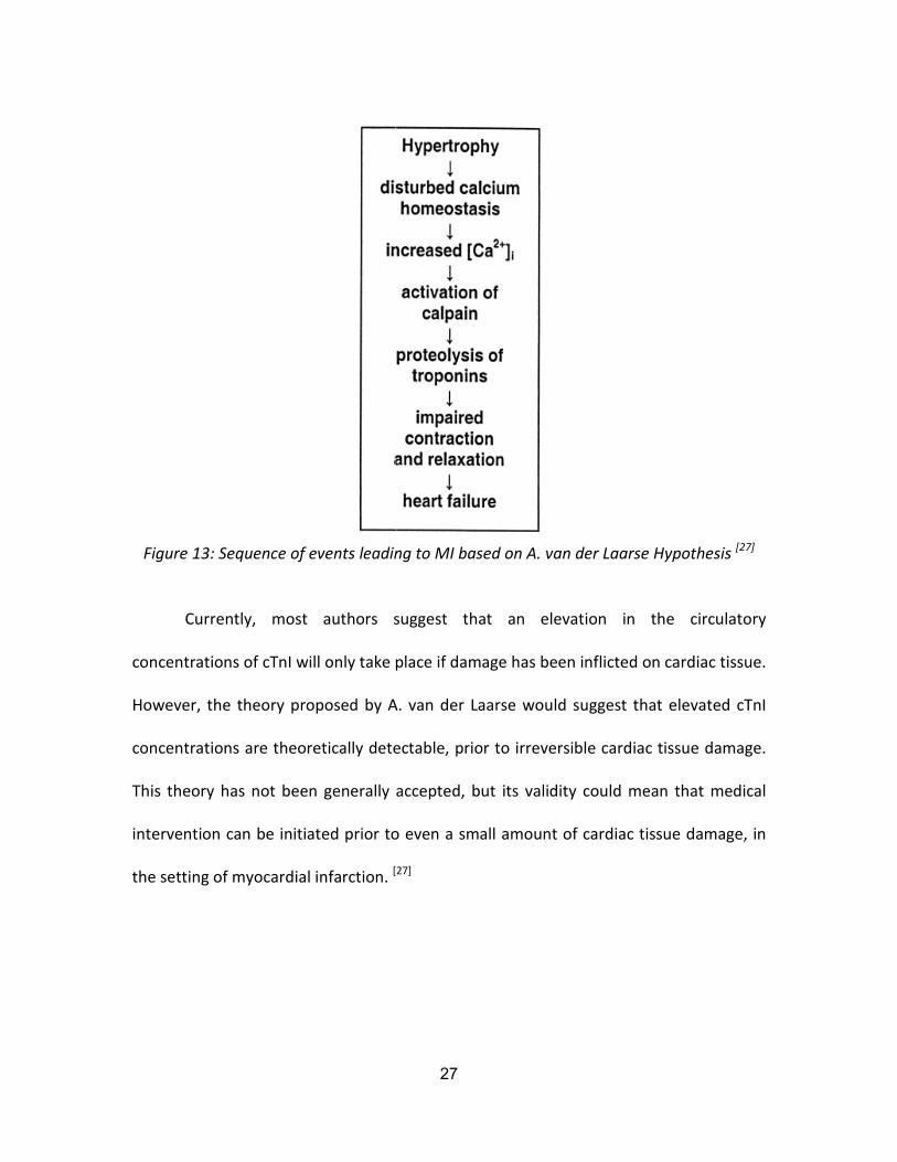
Figure 13: Sequence of events leading to MI based on A. van der Laarse Hypothesis [27]
Currently, most authors suggest that an elevation in the circulatory
concentrations of cTnI will only take place if damage has been inflicted on cardiac tissue.
However, the theory proposed by A. van der Laarse would suggest that elevated cTnI
concentrations are theoretically detectable, prior to irreversible cardiac tissue damage.
This theory has not been generally accepted, but its validity could mean that medical
intervention can be initiated prior to even a small amount of cardiac tissue damage, in
the setting of myocardial infarction. [27]

28
3. Raman Spectroscopy
3.1. Introduction and Background
Raman spectroscopy is a technology, principled on the quantitative
measurement of the wavelength and intensity of inelastically scattered light from
molecules. The Raman scattered light occurs at wavelengths that are shifted from the
incident light by the energies of molecular vibrations. This vibration can be observed in
either the Infrared (IR) or Raman Spectra. While IR spectroscopy measures the
absorption of infrared light by the sample, Raman spectroscopy measures the scattered
light.
In Raman Spectroscopy, the laser beam is used to irradiate the sample at UV-
Visible-NIR spectrum (200-900 nm). The scattered beams are also at UV-Visible-NIR
region and consist of two parts: Rayleigh scattering is strong and has the same
frequency as the incident beam, and Raman scattering is very weak and has a frequency
of higher or lower of the incident beam. These discrepancies in frequency of incident
beam and Raman scattering is unique to each molecule, allowing an ability to
confidently identify molecules through their characteristic properties. A Stoke is defined
as a Raman scatter frequency that is lower than the incident beam frequency; similarly
an Anti-Stoke is a Raman scatter frequency, higher than the initial incident beam.

29
As shown in equation 1, the Raman incident beam (V0) is shifted due to
molecular vibration and Stroke (V0-Vm) or Anti-Stroke (V0+Vm) results.
Force constant (K), and mass effect (µ), are both contributing factors that
determine vibration frequencies.
(EQ 1)
As previously mentioned, Raman spectroscopies are done in the UV region;
subsequently, IR and Raman are considered complementary in that certain vibrations
will be solely Raman active (e.g. totally symmetric vibrations), while others being
exclusively IR active. Covalent bonds are generally very strong in Raman while ionic
bonds are strong in IR. This feature of Raman makes it especially advantageous for our
studies of proteins as it can adequately detect the vibration of the covalent bonds
between the amino acids. Moreover, since the laser beam is about 1-2 mm, only a very
small sample is needed for detection, further serving as an advantage over IR for our
research purposes. Another advantage of Raman over IR spectroscopy is that proteins in
the body are in an aqueous solution and IR is inconveniently, a strong absorber of water.
On the contrast, water is a weak Raman scatterer. Once again, this inherent quality
deems Raman a superior choice for bioscientific application. Lastly, with regards to
instrumentation, Raman shift ranges from 4000 to 50 cm-1 and can be observed using a

30
single recording while gratings, beam splitters, filters and detectors must all be changed
to cover the same range while operating IR spectroscopy.
3.2. Literature Review
The incident wavelength was chosen to be at 785 nm, as typically used in
experimentation with organic compounds.[28] As shown in equation 2, the power of
Raman scatter is directly proportional to the intensity of the incident light, while
inversely proportional to the fourth power to the expectation wavelength. Thus, there is
a mathematical compromise that needs to be considered.
(EQ 2)
Because the Raman scatter is inversely proportional to the fourth power of the
excitation wavelength, more Raman scatter will be observed as the energy of excitation
wavelength increases. Therefore, as we lower the excitation wavelength, we see more
Raman back scattering. However, since the florescence region spans from 275 nm to
975 nm, we would promote florescence with sometime very strong signals that
completely overwhelm the Raman signals. Therefore, as we increase the excitation
wavelength, we see less florescence effect and at the same time we observe
attenuation in the power of Raman scattering. [28]

31
3.3. cTnI versus cTnT
As mentioned in the previous chapter, both cTnI and cTnT are specific cardiac
biomarkers that are released as part of the cTnI complex into the blood stream
following myocardial damages. For the purpose of this research we initially conducted
all of our experiments for both cTnI and cTnT. The Appendix includes a representative
portion of the results from cTnT Raman spectroscopy. However, during our literature
review process we discovered that cTnT forms different configurations after it is
released into the blood stream, which makes the concentration of a single isoform of
the protein even lower. An increase in the number of isoforms decreases the
concentration of each isoform. Since Raman is sensitive to each isoform, a progressive
decrease in the concentration of each form, secondary to this alteration in
configuration, resulted in a similarly progressive attenuation in Raman signal intensity.
This suboptimal characteristic of cTnT prevented us from further investigation of this
biomarker. The costume buffer containing the cTnI, used in this part of the project was
prepared based on a study by I.M. Vlasova. [29]
3.4. Remarks
3.4.1. Savitzky-Golay Filter
Savitzky-Golay smoothing filters (also called digital smoothing polynomial filters
or least squares smoothing filters) are typically used to "smooth out" a noisy signal

32
whose frequency span (without noise) is large. In this type of application, Savitzky-Golay
smoothing filters perform much better than standard averaging FIR (finite impulse
response) filters, which tend to filter out a significant portion of the signal's high
frequency content along with the noise. Savitzky-Golay filters are optimal in that they
minimize the least-squares error in fitting a polynomial to each frame of noisy data. [54]
3.4.2. Wavelet Transform
The Fast Wavelet Transform is a mathematical algorithm that facilitates changing
a waveform or signal that is originally in time domain into a series of coefficients. This
transformation is based on an orthogonal basis of small finite wavelets. Wavelet
transform can be simply applied to multidimensional signals, such as images, where the
time domain is replaced with the space domain. In this research Wavelet Transform is
used to analyze the Raman peaks of cTnI and BSA.
3.5. Spectral Result of Raman Spectroscopy Measurement of cTnI
In order to investigate the possibility of cTnI detection using Raman
spectroscopy, we designed and performed a number of experiments using various
Raman spectroscopes with different experimental set ups. In our first experiment, we
used a commercialized SpectraCode RP-1 Portable Raman Spectrometer, located at the
SFU Physics Department. Five different instruments where used during this research in

33
order to verify and confirm reproducibility of our results. The rest of the instruments
used in this research were generously provided by: The department of Chemistry (SFU),
National Research Council Canada (UBC), and the department of Chemistry, under
Professor Edward Grant Group (UBC).
This section outlines various results from the second set of experiments, which
was conducted using the two industrial and research Raman Spectrometers at UBC
Grant Groups Lab. A summary of many iterations, further measurements, as well as
verification results are presented in the next chapter. The apparatus setting for the
result of this section is as follows: laser excitation wavelength of 785 nm and the full
laser power of 140 mW. In each experiment an average of 30 trials are attempted, and
the background noise is subtracted from the collective signals. In this section, mouse
cTnI is diluted in a buffer solution of 200mL of 0.1M- KH2PO4 and 0.1M-NaOH. The raw
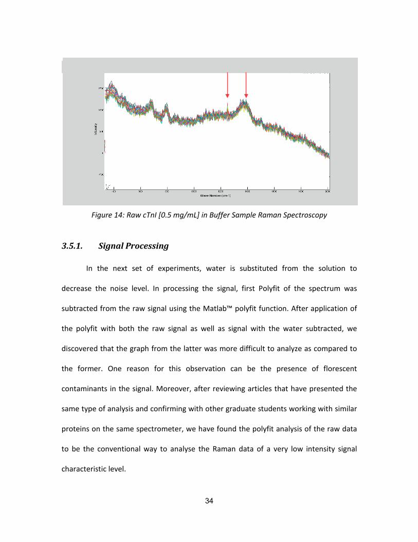
signal is presented in Figure 14.
34
Figure 14: Raw cTnI [0.5 mg/mL] in Buffer Sample Raman Spectroscopy
3.5.1. Signal Processing
In the next set of experiments, water is substituted from the solution to
decrease the noise level. In processing the signal, first Polyfit of the spectrum was
subtracted from the raw signal using the Matlab™ polyfit function. After application of
the polyfit with both the raw signal as well as signal with the water subtracted, we
discovered that the graph from the latter was more difficult to analyze as compared to
the former. One reason for this observation can be the presence of florescent
contaminants in the signal. Moreover, after reviewing articles that have presented the
same type of analysis and confirming with other graduate students working with similar
proteins on the same spectrometer, we have found the polyfit analysis of the raw data
to be the conventional way to analyse the Raman data of a very low intensity signal
characteristic level.

35
In Figure 15, the pink graph (polyfit data) is subtracted from the blue graph (raw
data), yielding the red line as the resulting graph. Final results are illustrated in Figure
16.
Figure 15: Polyfit subtraction steps for new cTnI.
Figure 16: SG Smoothing process for the cTnI
Polyfit cTnI Spectrum SG Smoothed Spectrum Subtracted de-noised, smoothed spectrum

36
Next Savitzky–Golay (SG), smoothing tools were applied to de-noise the data.
Then this graph was subtracted from the previous polyfit graph to remove the baseline.
3.5.2. cTnI Raman Signiture for the First Time
After conducting several iterations of cTnI signal processing and experiments, we
were able to characterize Raman signature of cTnI. To our knowledge, this is the first
time this has been reported in the scientific literature. Figure 17 outlines our findings.
Figure 17: First cTnI signature
We have compared the result of all 30 iterations of our experiment and have
consistently observed that the peak of 1700cm-1, is Raman’s peak for water and the
peaks between 1200 cm-1 -1400cm-1 are related to cTnI Raman signature as shown in
Figure 17.

37
3.5.3. Results and Discussions
Limited by the sensitivity and signal-to-noise ratio (SNR) of our first Raman
instrument, one of the main challenges in this research was the low intensity of the
different signals when the buffer Raman signature is subtracted from the cTnI raw
sample. These results carry a relatively large noise ratio compared to the signals that
were determinants of cTnI signature. Although difference amplitude in some regions of
the signal was observed, it was difficult to draw a conclusion to find the essential
difference.
As it will be presented in the following descriptive chapters, further investigation
and signal processing measures were carried through a combination of the latest Raman
instrument and chemometrics methods, which greatly improved the SNR of Raman
signal and made the differences more revealing. These new strategies, presented
herein, made the relationship between Raman spectral difference and cTnI intensity
more objectively evident.
Also from the Figure 17, we can conclude that despite the low intensity of the
signal, by characterizing the spectra, the change in concentration of cTnI can be
measured in the plasma or blood. These results were behind the motivation to continue
this research and further compare plasma from a normal mouse as well as a mouse,
which suffered from an MI. As it will be outlined, further experiments were conducted
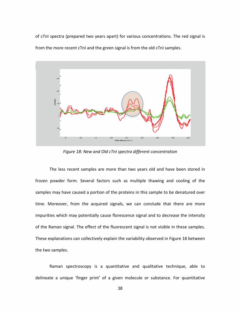
to identify the differences in the Raman signal peak. Figure 18 is an overlay of two types
38
of cTnI spectra (prepared two years apart) for various concentrations. The red signal is
from the more recent cTnI and the green signal is from the old cTnI samples.
Figure 18: New and Old cTnI spectra different concentration
The less recent samples are more than two years old and have been stored in
frozen powder form. Several factors such as multiple thawing and cooling of the
samples may have caused a portion of the proteins in this sample to be denatured over
time. Moreover, from the acquired signals, we can conclude that there are more
impurities which may potentially cause florescence signal and to decrease the intensity
of the Raman signal. The effect of the fluorescent signal is not visible in these samples.
These explanations can collectively explain the variability observed in Figure 18 between
the two samples.
Raman spectroscopy is a quantitative and qualitative technique, able to
delineate a unique ‘finger print’ of a given molecule or substance. For quantitative

39
molecular measurements of Raman spectroscopy, enhancing chemometric methods can
be supplemented for low sample concentrations. As previously discussed, florescence
can often contaminate Raman spectra. The use of a Near-IR 785 nm laser helps with
reduction of the possibility of fluorescent contamination; regardless, our sample still
contains a relatively large portion of fluorescent in the signal, which can cause photo
bleaching and saturation, resulting in the Raman signal to be quenched. Therefore, even
though we can conclude that cTnI Raman is quantitative, the relationship between the
change in concentration of cTnI and its Raman signal is not linear; the inconsistency
between the increase in sample concentration and sensitivity of detection suggests the
ultimate need for a yet more sensitivity apparatus. In general, despite the low
magnitude of signal characteristics, we are confident that the signature peaks are
identifiable after signal processing as well as utilizing more precise instruments.

40
4. Verification of cTnI Signature
4.1. Experiment procedure
In order to replicate and verify the unique Raman signature of cTnI discussed in
our previous chapter, an experiment was conducted on mouse cTnI to find its Raman
spectra. The specifications of the Raman Spectrometer instrument used for this
experiment are as follows: wavelength is 785 nm and the full laser power is 140 mW.
For the particular measurement presented in this report, the integration time is 5
seconds and 2 seconds. In previous experiments, the background noise of the spectrum
was removed, wavelet transform was performed and the portion of the wavelength
related to cTnI was extracted. However, when whole mouse serum was analyzed, the
resulting signal contained excessive noise caused by various components in the blood as
outlined previously. Therefore, it was concluded that without completely characterizing
the protein, conducting an experiment in the blood is not possible with the available
technology. Therefore, the first step towards implementation of this project is to verify
the cTnI spectra in water.
The research in this report is conducted in a completely different experimental
environment, consisting of new samples and instruments, as compared to previous

41
experiments. More specifically, the results presented in the following section have been
generated from a 20mg/mL mouse cTnI sample in double distilled water.
4.2. Verification Result and Discussion
Figure 19 represents data acquired from double distilled water and a 20 mg/mL
cTnI for the purpose of verification of previous finding in the same research.
Figure 19: Water and cTnI sample after noise reduction.
Figure 20 provides a comparison between various noise reduction levels of
adjusted cTnI spectra.

42
Figure 20: Different levels of Smoothing of water and sample.
Figure 21 illustrates a snapshot of the part of cTnI signal with more characteristic
peaks at various noise reduction and smoothing levels.

43
Figure 21: Snapshot of cTnI sample subtracted from water signal.
From the above graph we can conclude that polynomial fit of smoothing level
using sgloay() function in Matlab presents the optimal noise reduction at level 6.
Therefore, this level of noise reduction was used throughout this project.
4.2.1. Effect of change in concentration
Figure 22 illustrates the effects of concentration change on the adjusted cTnI
sample using 5 seconds integration time. It can be confirmed from this graph that the
intensity of the Raman spectra elevates as the concentration of cTnI the increases.
Figure 22: Effect of change in concentration, adjusted cTnI, 5 seconds integration time

44
4.2.2. Comparison with Previous Results
A close up of cTnI sample spectra is shown in Figure 23, which demonstrates the
same signature presented in previous findings (shown Figure 24). We believe the region
defined within the circle on the graph is the signature associated with cTnI in aqueous
solution. This characteristic was seen with various concentrations of the samples.
Figure 23: cTnI signature.
Figure 23 verifies previous findings regarding the location of cTnI signature, and
serves as further indication that the protein can be characterized using Raman
spectroscopy.

45
Figure 24: Previous results for cTnI signature.

46
5. The latest Spectral Result of cTnI in BSA
The novelty of this research is the fact that for the first time Raman spectroscopy
of cTnI is observed and documented through designing and performing a series of
experiments. After re-evaluating and reproducing the cTnI Raman signature in the
previous chapter, in this section our final experimental result is presented. Herein, we
identify the exact position of the mouse wild type non-phosphorylated cTnI peaks when
measured in Bovine Serum Albumin (BSA). Moreover, results in this chapter define a
boundary for concentration, as well as integration time conditions for future
instrumentation purposes of this research.
5.1. Results and Discussions
In order to further verify the possibility of cTnI measurement using Raman
spectroscopy, we designed and performed a number of experiments in various
experimental environments and conditions. As stated in the previous section, we
continued the assessment after we verified the cTnI signature. This section presents
various results from the latest set of experiments. Further measurements on several
iterations of different concentrations of cTnI and BSA in water are shown in the
following figures. The experiments presented in this section are measured with a new
Raman spectroscopy device and the apparatus setting is as follows: laser wavelength of

47
785 nm and the full laser power of 140 mW. Moreover two types of cTnI samples in
various concentrations were used for all of the following experiments (marked as cTnI[1]
and cTnI[2]) in order to verify that the observed peaks are validly related to the cTnI
protein. cTnI[2] is a more recently synthesized protein and the date of preparation is
September 14, 2011 as compared to cTnI[1] which was prepared on March 24, 2009,
and stored in powder form since then.
Figure 25 illustrates the raw cTnI, BSA and water spectra. These spectra can be
used to initially distinguish between the three samples and pinpoint the visible
differences in the signals.
Figure 25: Raw samples of BSA [20 g/L] , cTnI(1) [17 g/L] and Water
Based on differences in the raw spectra of cTnI and BSA in the above figure, we
have concluded that by performing signal processing of the spectra, a unique

48
characteristic of the signal can be extracted and used as detection strategy to
distinguish cTnI from the noise.
5.1.1. Effects of Change in integration time
Figure 26 and Figure 27 present the change in concentration of the cTnI sample
spectra with respect to change in integration time.
Figure 26: Change in integration time of cTnI(2) [13 g/L]

49
Figure 27: Change in integration time for adjusted cTnI spectra (cTnI(1) [14 g/L]/BSA [3.5 g/L]), (cTnI(1) [12 g/L]/BSA [6 g/L]), (cTnI(1) [10 g/L]/BSA [8 g/L]), (cTnI(2) [10 g/L]/BSA
[5 g/L])
From Figure 26 and Figure 27, it can be appreciated that as the integration time
decreases, the signal-to-noise ratio is also decreased. Other than the effect of signal to
noise ratio, we have observed that when the laser is on the sample for 60 seconds or
longer, the signal intensity decreases. This can be explained by the degeneration of the
cTnI sample, secondary to heating from the laser. This degeneration does not
compensate for the increased SNR and we can conclude that increasing the integration
time is a compromise. Therefore, for the purpose of this research 30 seconds of
integration time reproduces the most optimal results.

50
5.1.2. Effect of Change in concentration
Figure 28 represents processed data for increasing concentration of new cTnI
samples. It can be noted from the graph that the signal intensity increases as the
concentration of cTnI is increased. However, this relationship is non-linear and when the
concentration of the protein is increased by 10 fold, the signal intensity does not
increase by the same amount.
Figure 28: Change in concentration of cTnI in water and BSA sample (30 sec. integration
time)
Therefore, even though we can conclude that cTnI Raman is quantitative, the
relationship between the change in concentration of cTnI and its Raman signal is not
linear and the intensity increase with the change in concentration is not very evident
which again calls for a more sensitive signal processing method. Moreover, the black
line in Figure 28 which represents the cTnI[2] Sample (the newly prepared cTnI) has a

51
relatively higher intensity compared to cTnI[1]. In fact, the more recently prepared
sample has undergone less degeneration, providing a stronger detected signal. This
further reiterates the fact that higher concentrations of the protein are directly
correlated with higher intensity of the raw spectra.
5.1.3. Adjusted cTnI Spectra
In this section, signals are presented after deduction of noise caused by BSA in
the sample. Further, the spectra are presented in Figure 29 after smoothing and
filtration.
Figure 29: Change in concentration for adjusted cTnI spectra (30 sec. integration time)
From the above graph it can be noted that the peaks related to cTnI are not
visible without performing signal processing. Limited by the sensitivity and SNR of the
current Raman instrument, the difference signal carries a large noise ratio. Although,

52
slight amplitude differences in some regions of the signal are observed, it is difficult to
conclude an essential difference. Further investigation and signal processing can greatly
improve the SNR of Raman signal and make the difference more revealing. The new
strategy will make the relationship between Raman spectral difference and cTnI
absorption more clear and convincing.
Figure 30: cTnI signiture zone, Change in integration time for adjusted cTnI spectra
(cTnI(1) [10 g/L]/BSA [8 g/L])
As it will be shown in the wavelet transform result in the next section, the two
unique windows related to cTnI’s unique signature are between 1237 cm-1 to 1303 cm-1,
and 1375 cm-1 to 1450 cm-1.

53
5.2. Wavelet Transform
The following experiments are performed using an industrial Raman
spectrometer, located at the UBC Grant Group Laboratory, using a 785 nm laser with full
laser power at 140mW. The analyzed data in the following graphs represent the
subtracted, averaged, and de-noised version of the raw cTnI spectra. Moreover, wavelet
transform analysis has been performed on the results for easier distinction between the
peaks of interest.
Figure 31 illustrates the Fast Wavelet Transform result for water, BSA and cTnI. It
can be seen that this method creates a frame of reference to compare the spectra.
Figure 31: FWT Raw samples of BSA [20 g/L] , cTnI(1) [17 g/L] and Water

54
5.2.1. Effect of Change in integration time
After a series of literature review on the Raman signal processing of biological
compounds, we have found the polyfit analysis of the raw data to be the conventional
way to analyse the Raman data of a very low intensity signal level.
After finding the polyfit spectra, this signal was subtracted from the raw spectra
of cTnI in order to reduce all signals to the baseline for easier comparison. In addition,
Savitzky–Golay (SG) smoothing tools were used to de-noise the data using sgolay()
function in Matlab.
Figure 32 and Figure 33 illustrate the effect of change in the integration time on
the fast wavelet transform processed cTnI spectra.
Figure 32: FWT Change in integration time of cTnI(2) [13 g/L]

55
Figure 33: FWT Change in integration time for adjusted cTnI spectra (cTnI(1) [14
g/L]/BSA [3.5 g/L]), (cTnI(1) [12 g/L]/BSA [6 g/L]), (cTnI(1) [10 g/L]/BSA [8 g/L]), (cTnI(2) [10 g/L]/BSA [5 g/L])
These graphs indicate that after performing the wavelet transform on the same
signals with different integration time, only the SNR changes with no appreciable
changes to the peak. Therefore, collectively from the new experiments as well as the
previous experiments on changing the laser power for the same measurements, we can
conclude that the experimental conditions such as laser power and integration time do
not affect the positioning of the peaks of interest.
5.2.2. Effect of Change in concentration
Figure 34 is an overlay of both old and new cTnI spectra for various
concentrations. The black signal is from the new cTnI and other signals are from
different concentrations of cTnI samples. The graph shows that Raman intensity of the

56
cTnI[1] sample at various concentrations does not demonstrate a large change in the
intensity after the wavelet transform is performed.
Figure 34: FWT Change in concentration of cTnI in water and BSA sample (30 sec.
integration time)
Considering the graph above, it can be noted that even though the concentration
of the old cTnI samples were higher than the newer samples, the intensity is lower. A
possible explanation for this is that the amount of impurities was larger with more
denaturation of the proteins in the old cTnI samples. However, this result is only valid to
a point where the concentration and SNR allows for detection of cTnI. The peaks change
as the noise level increases and cTnI peaks are not visible. In all of the experiments
conducted for this research, we can measure the cTnI protein in concentrations 100
times higher than physiological concentrations.

57
5.2.3. Adjusted cTnI Spectra
As previously mentioned, the purpose of this research is to find the unique
Raman signature of cTnI to be later used as a mean for early prediction of myocardial
infarction. Figure 35 present the fast wavelet transform of various concentrations of
cTnI sample (cTnI -BSA samples after subtraction of BSA) and the BSA spectrum shown
in blue. Segments of cTnI spectra, determinant of the protein’s signature and its
intensity, are above that of BSA and can be seen in Figure 35 for all cTnI concentrations.
Figure 35: FWT Change in concentration for adjusted cTnI spectra (30 sec. integration
time)
Figure 36, shows the overlay graph of various concentrations of cTnI and BSA
spectra in the 1200 cm-1 to 1470 cm-1 window where most of the cTnI characteristic
resides. From the results in this section, it can be deduced that both the wavelet

58
transformed data and raw signals are required to be able to first locate the exact peaks,
and detect the concentration increase.
Figure 36: FWT Change in integration time for adjusted cTnI spectra (cTnI(1) [10
g/L]/BSA [8 g/L])
As demonstrated in Figure 36, the two smallest windows related to cTnI’s unique
signature is between 1237 cm-1 to 1303 cm-1 and 1375 cm-1 to 1450 cm-1. These results
verify the possibility of extracting cTnI spectra from BSA, which is one of the larger
proteins that can be used as an arbitrary noise. Arguably, BSA was a logical next step
after experimentation in water, before this apparatus can be optimized for detection of
cTnI in intact human blood.

59
5.3. Discussion and Conclusion
Figure 38 illustrate discrepancies between peaks present on the BSA and water
Raman scattering of cTnI. These peaks were analyzed using existing literature, amino
acid sequence and protein foldings. The region outlined in the figure (approximately
600 cm-1) demonstrates three peaks in BSA Raman signals, which are absent in water
and cTnI. One possible explanation for this inconsistency is the presence of disulfide
bonds in BSA, which are nonexistent in the water and cTnI. In fact, BSA contains 17
disulfide bridges from residues 77 to 590.
Further, the arrow indicating the region at approximately 850 cm-1 may be
secondary to the presence of Tyrosine (Try). BSA contains 21 tyrosines (3.5% of the
amino acids) while cTnI contains 4 Try (1.9% of amino acids). While the orientation,
different substitution symmetry and neighbouring amino acids might shift signals and
alter the intensities; a sharp peak observed at the region is characteristics of Tyrosine.
[30]

60
Figure 37: cTnI and BSA Raman Peak Analysis
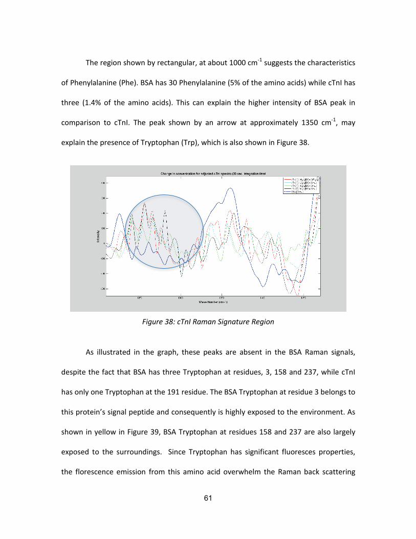
61
The region shown by rectangular, at about 1000 cm-1 suggests the characteristics
of Phenylalanine (Phe). BSA has 30 Phenylalanine (5% of the amino acids) while cTnI has
three (1.4% of the amino acids). This can explain the higher intensity of BSA peak in
comparison to cTnI. The peak shown by an arrow at approximately 1350 cm-1, may
explain the presence of Tryptophan (Trp), which is also shown in Figure 38.
Figure 38: cTnI Raman Signature Region
As illustrated in the graph, these peaks are absent in the BSA Raman signals,
despite the fact that BSA has three Tryptophan at residues, 3, 158 and 237, while cTnI
has only one Tryptophan at the 191 residue. The BSA Tryptophan at residue 3 belongs to
this protein’s signal peptide and consequently is highly exposed to the environment. As
shown in yellow in Figure 39, BSA Tryptophan at residues 158 and 237 are also largely
exposed to the surroundings. Since Tryptophan has significant fluoresces properties,
the florescence emission from this amino acid overwhelm the Raman back scattering

62
which results in absents of these peaks as number of Tryptophan residues increase in a
protein.
The interpretations of these peaks are based on the current literature. [30]
Considering the limited number of scientific studies published on the topic, further
reports are necessary to confirm these findings. Moreover, due to the particular
sensitivity of Raman spectroscopy to orientation and protein folding, the associated
wave numbers are only approximate and must be further researched using more
intricate equipment.
Figure 39: The Tertiary structural model of BSA

63
6. Conceptual Design of Raman Detection of cTnI System
6.1. Literature Review
To our knowledge the most similar technological design to our concept is one
patented by Anthony J. Durkin in 2004. This patent utilizes Raman spectroscopy through
the human eye and is designed as a glucose monitoring device, intended for
management of Diabetes Mellitus. This device provides further encouragement for our
eventual goal of concept implementation in the setting of MI. Figure 40 is a
representative diagram, outlining the principles behind this patent. Through this device,
Raman spectroscopy is used “to non-invasively detect the molecular characteristics [as
well as] constituents of the aqueous humor, vitreous humor, lens or retina”. [34] Through
a step wise apparatus, light is introduced into the patient’s eye using laser, Raman
spectra are collected onto the detector and analyzed, and the detected spectra are used
for identification of molecular changes. [34]
Our intended future approach is similar to the mentioned system; differences
included our intended collection site, which is the area in the back of the human eye, on
the surface of the retina and close to the optical nerve, which serves as the only area of
the body where blood vessels can be directly visualized. In fact, this strategic area is
routinely visualized by ophthalmologists in patients with high blood sugar levels in order

64
to assess the extent of direct damage to the vessels from states of chronic
hyperglycemia. For experimental purposes, we can integrate principles from confocal
microscopy in order to focus the laser as a specified blood vessel on the retina and
obtain signals from this selected region of interest. [34]
Figure 40: Patent diagram of Raman Spectrometer for Glucose Measurement form
Human Eye [34]
6.2. Conceptual Design of Raman Detection of cTnI System
The focus of this research so far has been on finding the Raman spectrum of cTnI.
The last part of the proceeding research is based on designing a conceptual proof of
concept for a device to be used as Raman spectroscope for measuring cTnI from the
eye. Figure 41 diagrams anatomical landmarks in the human eye, illustrating the
minimal barriers between the external environment and visualization of internal blood

65
vessels. This unique anatomical feature of the eye is used commonly in clinical diagnosis
and also allows optimal implementation for our project as the retinal vasculature can
serve as a good platform for spectroscopic reading. In addition to the vascularity, the
transparent nature of the aqueous humour further aids device implementation.
Figure 41: Anatomy of the eye [35]
Figure 42 further demonstrate the abundance of blood vessels in the region
juxtaposed and overlying the entrance of the optic nerve into the eye. Due to inherent
anatomical characteristics of the retina and image processing of the eye, this region of
the retina does not contain any photoreceptors and is often called the “blind spot”; this
characteristic is beneficial in our device will likely be more safe for use if the laser

66
applied for detection does not come in contact with the natural photoreceptors of the
eye and utilizes vessels from the blind spot.
Figure 42: Optic Nerve, Sampling point of interest [36]
Figure 43 presents a potential Raman spectroscopy configuration in the human
eye. A major difference between our illustrations as compared to that depicted in Figure
40 is that the former is focused at a specific point on a chosen vessel whereas the latter
is full field focused.

67
Figure 43: Possible Raman Spectroscopy configuration for conceptual system. In this
configuration, DG stands for Diffraction Grating, LPDF for Long Pass Dichroic Filter, and BP for Band pass Filter.
Figure 44 presents a combination of subsystems, which can be used as our
conceptual design and only uses Raman spectroscopy. The sample arm is used to find
the point of interest to focus on, which in this case will be the optimal blood vessels
near the optic nerve.

68
Figure 44: Overall Conceptual Optical Configuration
Finally, Figure 45 presents part of an overall conceptual design of the system.
The excitation beam will be transmitted (in a short pulse form) from a small laser diode
through the pupil and on to the retina. Consequently, the emission light is reflected
back through the pupil and to a small prism, which in turn will reflect the light to a
miniaturized CCD camera for measurement.
Raman
Output

69
Figure 45: Conceptual Design of the system

70
7. Conclusion
The ultimate goal of this project was to decrease morbidity, mortality and the
significant burden of disease associated with MI, using novel technology. Our very first
design envisioned a device capable of wirelessly and continuously monitoring, recording
and analyzing ECG readings from high-risk patients. The concept included ability for the
device to automatically contact emergency crew with an abnormal reading. This concept
was soon abandoned, realizing the relative lack of sensitivity and specificity associated
with ECG readings in the setting of an MI. We consequently re-designed our concept,
implementing florescence spectroscopy. Cardiac biomarkers are clinically and
diagnostically superior to ECG readings, and were the most logical indicators of MI for
the apparatus to detect; therefore, an attempt was made to detect cTnI concentrations
using florescence spectroscopy. The Tryptophan amino acid in the protein sequence of
cTnI was hypothesized to provide unique molecular florescence characteristics.
However, limitations in currently available technology prevented us from successfully
obtained a unique spectrum. Finally, in the current project, Biophotonics measurements
of cTnI were successfully utilized as extensively discussed. Through this project, and to
our knowledge for the first time in literature, we consistently characterized the unique
Raman spectrum of mouse cTnI protein. This spectrum was verified several times and in
different experimental and analytical settings, initially in water and subsequently in BSA.

71
Our choice of BSA as the experimental milieu represented its structural similarity to
intact blood and served as a progressive step prior to apparatus optimization in human
blood. The two narrowest and most consistently verified windows, relating to the
unique spectrum of cTnI in BSA are between 1237 cm-1 to 1303 cm-1 and 1375 cm-1 –
1450 cm-1.
However, we still face sensitivity limitations with our apparatus and the lowest
concentrations of cTnI at which we were able to accurately characterize Raman peaks
were one hundred times the physiological concentrations. Our approach to minimize
this limitation was to enhance the signal to noise ratio (SNR) of the spectrum, through a
wavelet transform analysis as discussed. We further optimized the apparatus by
discovering that an attenuation of the integration time to as low as 2 seconds do not
effectively alter our results and this finding will be beneficial in the latter instrument
optimization and standardization stages of the project. Our results indicate that both
wavelet transformation data as well as raw Raman signaling data are necessary in order
to detect associated peaks as protein concentrations increase. We further learnt that
under in vitro settings, changes in integration time with respect to Raman signal
intensity is not linear, likely secondary to the degenerative effects of heating from the
exposure to the laser, on the cTnI protein. Similarly, changes in concentration with
respect to Raman signal intensity is not linear, secondary to the fact that our
instruments are unable to linearly decrease block florescence signals, with linear
decrease of cTnI concentrations. Perhaps, more advanced signal processing and CCD

72
cameras can further improve the SNR as well as the sensitivity of the apparatus to more
physiological concentrations. In addition to this, further goals of this project include
device miniaturization and calibration. The finalized device can eventually be
supplemented by telemedicine ECG measurements as briefly discussed above, in order
to serve as a comprehensive and non-invasive diagnostic apparatus for MI.

73
8. References
1. D. Lloyd-Jones et al. “Lifetime risk of developing coronary heart disease.”
The Lancet, Vol. 353, Issue 9147, pp. 89 - 92, Jan. 1999.
2. D. Cullen et al. “Therapeutic Hypothermia Initiated in the Pre-Hospital
Setting: A Meta-Analysis.” Advanced Emergency Nursing Journal, Vol. 33, pp. 314–
321, Dec. 2011.
3. C. Baigent. “10 year survival among patients with suspected acute
myocardial infarction in randomised comparison of intravenous streptokinase, oral
aspirin, both, or neither”. BMJ, pp. 316:1337, May 1998.
4. E. Braunwald. “Biomarkers in Heart Failure”. N Engl J Med. Vol. 358, pp.
2148-2159, May 2008.
5. H. B. A. Wu. “Gender-Specific Decision Limits for Cardiac Troponin for Risk
Stratification?”International Anesthesia Research Society, 2009.
6. A. Hans-Richard Arntz et al. “Initial management of acute coronary
syndromes.” European Resuscitation Council Guidelines for Resuscitation. pp. 1353 –
1363, Oct. 2010,

74
7. T. Reichlin, et al. “Early Diagnosis of Myocardial Infarction with Sensitive
Cardiac Troponin Assays”. N Engl J Med, vol 361, pp. 858-867, Aug. 2009.
8. A. Rasekh, M. Razavi and A. Massumi, “Sudden Cardiac Death”.
Cardiovascular Medicine, Sec. IX, pp. 2039-2083, 2007.
9. H.M. Piper, Y. Abdallah and C. Schäfer, “The first minutes of reperfusion: a
window of opportunity for cardioprotection”. European Society of Cardiology, 2003.
10. P. Anversa, and E. Sonnenblick, “Ischemic cardiomyopathy:
pathophysiologic mechanisms.” Prog Cardiovasc Dis., vol. 33, pp. 49-70, 1990.
11. S. Moghaddamjoo, “Prediction Of Myocardial Infarctions, Using Non
Invasive Biophotonics Measurement Of Cardiac Troponin I”, Thesis Submitted to
Simon Fraser University Library, Dec. 2010.
12. L.M. Buja, “Myocardial ischemia and reperfusion injury”. Cardiovascular
Pathology, vol. 14, issue 4, pp 170–175, Aug. 2005.
13. G. Ermak, and K. Davies, “Calcium and oxidative stress: from cell
signalling to cell death”. Molecular Immunology, vol. 38, issue 10, pp713–721, Feb.
2002.
14. D.M. Bers, S. Despa and J. Bossuyt, “Regulation of Ca2+ and Na+ in Normal
and Failing Cardiac Myocytes”. Annals of the New York Academy of Sciences, vol.
1080, pp. 165–177, Oct. 2006.

75
15. A. G. Katrukha et al. “Degradation of cardiac troponin I: implication for
reliable immunodetection.” Clin Chem vol. 44 pp. 2433–440, 1998.
16. G. Lum, D. Solarz and L. Farney. “False Positive Cardiac Troponin Results
in Patients Without Acute Myocardial Infarction”. American Society for Clinical
Pathology, Mar. 2006.
17. Q. Shia et al. “Degradation of Cardiac Troponin I in Serum Complicates
Comparisons of Cardiac Troponin I Assays”. Clinical Chemistry, vol. 45, no. 7 pp.
1018-1025, Jul. 1999.
18. D. I. Ellis and R. Goodacre, “Metabolic fingerprinting in disease diagnosis:
biomedical applications of infrared and Raman spectroscopy,” Analyst, 2006.
19. The Encyclopaedia of Science, “Tryptophan”. Internet:
http://www.daviddarling.info/encyclopedia/T/tryptophan.html [Mar. 23, 2012]
20. Microscopy Resource Center. “Olympus Microscopy Resource Center”.
Internet: http://www.olympusmicro.com/primer/anatomy/sources.html [Apr. 15,
2009]
21. J. S. Alpert et al. “Myocardial infarction redefined: A consensus document
of The Joint European Society of Cardiology/American College of Cardiology
Committee for the redefinition of myocardial infarction”. Journal of American College
of Cardiology, vol 36, pp. 959-69, 2000.

76
22. K. Hideo and K. Hirose. “Diagnostic accuracy of cardiac markers for
myocardial damage after radiofrequency catheter ablation”. Journal of Interventional
Cardiac Electrophysiology, pp. 169-174, 2009.
23. D. C. Collinson. “Multiple molecular forms of circulating cardiac troponin:
analytical and clinical significance”. Association for Clinical Biochemistry. , pp. 349–
355. 2008.
24. D. Ward, M. Cornes, I. Trayer. “Structural Consequences of Cardiac
Troponin I Phosphorylation.” The American Society for Biochemistry and Molecular
Biology, Aug. 2002.
25. A. G. Katrukha et al. “Degradation of cardiac troponin I: implication for
reliable immunodetection”. Clin Chem. vol. 44, pp. 2433–440, 1998.
26. R. Labugger et al. “Extensive troponin I and T modification detected in
serum from patients with AMI.” Circulation, vol. 102, pp. 1221–1226, 2000.
27. A. Van der Laarse. “Hypothesis: troponin degradation is one of the factors
responsible for deterioration of left ventricular function in heart failure.”
Cardiovascular Res. vol. 56, pp. 8–14, 2002.
28. Laser Focus World, “The American Society for Biochemistry and
Molecular Biology”, Feb. 2012.

77
29. I.M. Vlasova and A.M. Saletsk. “Raman spectroscopy in investigations of
mechanism of binding of human serum albumin to molecular probe fluorescein”.
Moscow: Lomonoaoy Moscow State University. vol 5, Issue 5, 2008.
30. A. Jenkins, R. Larsen and T. Williams, “Characterization of amino acids
using Raman spectroscopy”. Spectrochimica Acta. vol. 61, pp. 1585–1594, 2005.
32. A. Durkin, E. Marwood and C. Vivian, “Method for non-invasive
identification of individuals at risk for diabetes.” United States. Patent No. US
6,721,583 B1, 2004.
33. Virtual Medical Centre. “Anatomy of the eye and visions.” Internet:
http://www.virtualmedicalcentre.com/anatomy/the-eye-and-vision/28, 2012
[March 23, 2012]
34. National Eye Institute, Internet:
http://www.nei.nih.gov/health/eyediagram/index.asp , 2008 [March 23, 2012]
35. J. Evans et al. “Optical coherence tomography and Raman spectroscopy of
the ex-vivo retina.” Multimodal Biomedical Imaging IV, vol. 7171, pp. 13768-13784,
2009.
36. A. Hans-Richard et al. “Initial management of acute coronary syndromes.”
European Resuscitation Council Guidelines for Resuscitation, pp. 1353 – 1363, Oct.
2010.

78
37. R. Labugger et al. “Extensive troponin I and T modification detected in
serum from patients with AMI.” Circulation. vol. 102, pp. 1221–1226, 2000.
38. W. Neagoe et al. “Titin isoform switch in ischemic human heart disease.”
Circulation, vol. 106, pp. 1333-1341, 2002.
39. T.J. Wang “Significance of circulating troponins in heart failure: if these
walls could talk.” Circulation, vol. 116 pp. 1217-1220, 2007.
40. R. S. Vasan, “Inflammatory markers and risk of heart failure in elderly
subjects without prior myocardial infarction: The Framingham Heart Study.”
Circulation vol. 107, pp. 1486-1491, 2003.
41. R. Latini et al. “Prognostic value of very low plasma concentrations of
troponin T in patients with stable chronic heart failure.” Circulation, pp. 116: 1242,
2007.
42. A. M. Annika et al. “Blood analysis by Raman spectroscopy”. Optics letters,
vol. 27, issue 22, pp. 2004-2006, 2002.
43. F.S. Apple, “Cardiac Troponin Testing for Detection of Myocardial
Infarction. Minneapolis” Humana Press, 2008.
44. D. M. Char, E. Israel, and J. Ladenson, “Early laboratory indicators of
myocardial infarction,” Emergency Medicine Clinics of North America, 1998.

79
45. J. Clark. “Absorption Spectra-the beer-lambert law.”
http://www.chemguide.co.uk/analysis/uvvisible/beerlambert.html, 2007, [April
26, 2009]
46. D. C. Collinson. “Multiple molecular forms of circulating cardiac troponin:
analytical and clinical significance.” Association for Clinical Biochemistry, pp. 349–
355, 2008
47. V. R. Eisenman. “Are all troponin assays equivalent in the emergency
department?” Singapore Medical Journal , pp. 325-327, 2005.
48. G. D. Lewis et al. “Metabolite profiling of blood from individuals
undergoing planned myocardial infarction reveals early markers of myocardial
injury.” Bioinformatics, vol 26, Issue 14, pp. 3503–3512, 2008.
49. K. P. Soreng, “Troponin I and troponin T in myocardial infarction diagnosis
and risk assessment.” Tarrytown, Bayer HealthCare LLC Diagnostics Division, 2008.
50. J. R. Lakowicz. Principles of Florescence Spectroscopy. New York: Springer.
2002.
51. S. Nie and S. R. Emory, “Probing Single Molecules and Single
Nanoparticles by Surface-Enhanced Raman Scattering.” Science, vol. 275, issue 5303,
pp. 1102-1106, 1997.

80
52. S. A. Takeda et al. “Structure of the core domain of human cardiac
troponin in the Ca2+- saturated form,” Nature, 2003.
53. World Health Organization, “Deaths by cause, sex and mortality stratum
in WHO regions,” The world health report, 2004.
54. Savitzky and M. J. E. Golay, "Smoothing and Differentiation of Data by
Simplified Least Squares Procedures," Analytical Chemistry, vol. 36, pp. 1627-1639,
1964.

81
9. Appendix
9.1. cTnT
“Figure 46 to
Figure 50 are the processed spectra of the samples. In these figures, the
spectrum of 10 trials for each concentration is averaged and the background noise is
subtracted from the signal. As mentioned in previous sections with respect to
sensitivity and specificity cTnT possess similar characteristics to cTnI, therefore we
acquired spectrum form this protein as well. The significance of analyzing cTnT in
both the costume made buffer and BSA is to get insight on the differences between
cTnI and cTnT and possibly investigate advantages of cTnT over cTnI for our
purposes”.[11]

82
Figure 46: 10 mg/mL cTnI in Buffer Sample Raman Averaged
Figure 47: 0.49 mg/mL cTnI in Buffer Sample Raman Averaged
500 1000 1500 2000 2500
8000
8200
8400
8600
8800
9000
Average spectra of BSA with 10mg concentration(A)
500 1000 1500 2000 2500
8000
8200
8400
8600
8800
9000
(B) Average spectrum of CTnI with 0.49 concentraion
Raman Shift (cm-1)
Raman Shift (cm-1)

83
Figure 48: 0.25 mg/mL cTnT in Buffer Sample Raman Averaged
Figure 49: Difference between BSA and cTnI Raman signals
500 1000 1500 2000 2500
8000
8200
8400
8600
8800
9000(C) Average spectrum of CTnT with 0.25 concentration
500 1000 1500 2000 2500 3000-60
-40
-20
0
20
40
60
(D) Difference between CTnI and BSA
Raman Shift (cm-1)
Raman Shift (cm-1)

84
Figure 50: Difference Between cTnT and Buffer Raman Signal
9.2. Florescence Experiment Set Up
Figure 51: Optical Florescence Experimental Setup
500 1000 1500 2000 2500
-20
0
20
40
60
80
100
120
140 (E) Difference between CTnT and BSA
Raman Shift (cm-1)

85
Figure 52: Physical set up for florescence
Figure 53: Physical set up for absorption

86
9.3. Florescence Spectroscopy
“Using the result acquired from the PTI Quantamaster UV-Vis
Spectrofluorometer of a complete scan through the cTnI sample, the excitation
wavelength of the protein was acquired. As illustrated in Figure 54, the excitation
wavelength of cTnI is 283 nm as expected from the existence of Tryptophan”.[11]
Excitation Graph 4000000 3000000 2000000 1000000 0
Wavelength (nm)
Figure 54: Scan through cTnI sample to find the excitation wavelength
“The data graph of the emission of cTnI sample when excited at 280nm is
shown in Figure 55. The peaks at higher frequencies than expected are artifacts due
to PTI Quantamaster Spectrofluorometer performance since they have also
appeared when scanning the negative control (water). The emission wavelength
for different concentrations of cTnI in water happens at 347 nm as expected. The
device again causes the second peak, which appears at higher wavelength. Table 5
summarizes the peak values at various concentrations.”[11]
200
221
242
263
284
305
326
347
368
389
410
431
452
473
494
515
536
557
578
599
620
641
662
683
704
725
746
767
788
809
830

87
Figure 55: The emission wavelength at different concentrations when excited at 283nm
Table 5: The peak values at various concentrations of cTnI
Molarity (uM) Peak Values 0 173657 18.96 2659630 21.44 2312060 24.73 2124130 28.03 1933120 33.39 1713940 41.22 1573370
The molecular weight of cTnI is 24,259 Da. Table 6 summarizes the molarity of
cTnI calculated using the molecular weight versus the absolute peak amplitude
of intensity (where peak value at zero concentration is subtracted from the rest of
the intensities). These values are plotted in Figure 56.

88
Table 6: The delta peak values at various molarities of cTnI
Molarity(uM) Delta Peak Amplitude(count/sec) 0 0
18.96 1399713 21.44 1540283 24.73 1759463 28.03 1950473 33.39 2138403 41.22 3485973
Figure 56: Absolute florescence intensity of various molarities of cTnI
In order to monitor the fluorescent behavior of the protein with an increase in
concentration, a linear regression analysis was performed (Figure 57). From the
regression analysis output, the slope of the line is 48252 counts/, the y-intercept is
529833.6 counts and the coefficient of determination (R2) is 0.95. This gives an
indication of the florescence characteristic of this protein with respect to increase in
concentration within the experimental and human error.[11]

89
Figure 57: Linear Regression Graph
The data presented in Table 7 was obtained at various concentrations.
Table 7: Absorption data
Power (uW) Concentration (uM) 1165 0.00 519 76.26 488 83.19 428 91.51 402 101.68 342 114.391 314 130.732 272 152.521 245 183.025 197 228.781
The absorption data is plotted in Figure 58. It can be seen that the power
versus concentration graph has a logarithmic behavior. Therefore we can conclude

90
the absorption characteristic is in agreement with the Beer-Lambert law as
expected, which is shown in the following equation.
Where I0 and I are the intensity (power) of the incident light and that after the
material, respectively.
Figure 58: Absorption characteristic

91
9.4. cTnI Amino Acid Sequence

92
9.5. BSA Amino Acid Sequence

93
9.6. BSA Sample Information

94
9.7. Sample Codes
clear all Spectrum1 = xlsread('CtNI5 3water BSA 15.xls'); Spectrum2 = xlsread('CtNI5 3water BSA 30.xls'); Spectrum3 = xlsread('CtNI5 3water 2BSA 15.xls'); Spectrum4 = xlsread('CtNI5 3water 2BSA 30.xls'); Spectrum5 = xlsread('CtNI5 3water3BSA 15.xls'); Spectrum6 = xlsread('CtNI5 3water3BSA 30.xls'); Spectrum7 = xlsread('CtNI5 3water3BSA 60.xls'); Spectrum8 = xlsread('ctni2 3x125 h2o then 1bsa 15.xls'); Spectrum9 = xlsread('ctni2 3x125 h2o then 1bsa 30.xls'); Spectrum10 = xlsread('ctni2 3x125 h2o then 1bsa 60.xls'); Spectrum11 = xlsread('ctni2 3x125 h2o 15.xls'); Spectrum12 = xlsread('ctni2 3x125 h2o 30.xls'); Spectrum13 = xlsread('ctni2 3x125 h2o 60.xls'); Spectrum14 = xlsread('BSA 15.xls'); Spectrum15 = xlsread('BSA 30.xls'); Spectrum16 = xlsread('BSA 60.xls'); Spectrum17 = xlsread('water.xls'); sample15=Spectrum5-Spectrum14; sample30=Spectrum6-Spectrum15; sample60=Spectrum7-Spectrum16; x=xlsread('WN.xls'); xx=(x(:,1)); figure %water, BSA, cTnI plot(xx,smooth(Spectrum17, 8,'sgolay'),'r','LineWidth',1.25); hold on plot(xx,smooth(Spectrum15, 8,'sgolay'),'b:');

95
hold on plot(xx,smooth(Spectrum2, 8,'sgolay'),'g'); xlabel('Wave Number (cm-1)','fontsize',14); ylabel('Intensity','fontsize',14); legend('Water','BSA [20 g/L]','cTnI(1) [17 g/L]','fontsize',14); title('Raw samples of BSA [20 g/L] , cTnI(1) [17 g/L] and Water','fontsize',14,'fontweight','b') axis tight; hold off %Change in integration time of cTnI in water figure plot(xx,smooth(Spectrum11, 8,'sgolay'),'r'); hold on plot(xx,smooth(Spectrum12, 8,'sgolay'),'b'); hold on plot(xx,smooth(Spectrum13, 8,'sgolay'),'g'); xlabel('Wave Number (cm-1)','fontsize',14); ylabel('Intensity','fontsize',14); legend('15 sec','30 sec','60 sec'); title('Change in integration time of cTnI(2) [13 g/L] ','fontsize',14,'fontweight','b') axis tight; hold off %Change in concentration time of cTnI in water and BSA figure plot(xx,smooth(Spectrum2, 8,'sgolay'),'r'); hold on plot(xx,smooth(Spectrum4, 8,'sgolay'),'b'); hold on plot(xx,smooth(Spectrum6, 8,'sgolay'),'g'); hold on plot(xx,smooth(Spectrum9, 8,'sgolay'),'k'); xlabel('Wave Number (cm-1)','fontsize',14); ylabel('Intensity','fontsize',14); legend('cTnI(1) [14 g/L]/BSA [3.5 g/L]','cTnI(1) [12

96
g/L]/BSA [6 g/L]','cTnI(1) [10 g/L]/BSA [8 g/L]','cTnI(2) [10 g/L]/BSA [5 g/L]'); title('Change in concentration of cTnI in water and BSA sample (30 sec. integration time)','fontsize',14,'fontweight','b') axis tight; hold off %Subtracted water and BSA from cTnI spectra (CtNI5 3water BSA) figure subplot(2,2,1) plot(xx,smooth(4.*Spectrum1-Spectrum14, 8,'sgolay'),'r'); hold on plot(xx,smooth(4.*Spectrum2-Spectrum15, 8,'sgolay'),'b'); hold on xlabel('Wave Number (cm-1)'); ylabel('Intensity'); legend('cTnI(1) [14 g/L]/BSA [3.5 g/L] 15 sec.','cTnI(1) [14 g/L]/BSA [3.5 g/L] 30 sec.'); title('Change in integration time for adjusted cTnI spectra (cTnI(1) [14 g/L]/BSA [3.5 g/L])') axis tight; hold off %Subtracted water and BSA from cTnI spectra (CtNI5 3water 2BSA) subplot(2,2,2) plot(xx,smooth(2.*Spectrum3-Spectrum14, 8,'sgolay'),'r'); hold on plot(xx,smooth(2.*Spectrum4-Spectrum15, 8,'sgolay'),'b'); hold on xlabel('Wave Number (cm-1)');

97
ylabel('Intensity'); legend('cTnI(1) [12 g/L]/BSA [6 g/L] 15 sec.','cTnI(1) [12 g/L]/BSA [6 g/L] 30 sec.'); title('Change in integration time for adjusted cTnI spectra (cTnI(1) [12 g/L]/BSA [6 g/L])') axis tight; hold off %Subtracted water and BSA from cTnI spectra (CtNI5 3water 3BSA) subplot(2,2,3) plot(xx,smooth(2.*Spectrum5-Spectrum14, 12,'sgolay'),'r'); hold on plot(xx,smooth(2.*Spectrum6-Spectrum15, 12,'sgolay'),'b'); hold on plot(xx,smooth(2.*Spectrum7-Spectrum16, 12,'sgolay'),'g'); xlabel('Wave Number (cm-1)'); ylabel('Intensity'); legend('cTnI(1) [10 g/L]/BSA [8 g/L] 15 sec.','cTnI(1) [10 g/L]/BSA [8 g/L] 30 sec.','cTnI(1) [10 g/L]/BSA [8 g/L] 60 sec.'); title('Change in integration time for adjusted cTnI spectra (cTnI(1) [10 g/L]/BSA [8 g/L])') axis tight; hold off %Subtracted water and BSA from cTnI spectra (ctni2 3x125 h2o then 1bsa) subplot(2,2,4) plot(xx,smooth(2.*Spectrum8-Spectrum14, 8,'sgolay'),'r'); hold on plot(xx,smooth(2.*Spectrum9-Spectrum15, 8,'sgolay'),'b'); hold on plot(xx,smooth(2.*Spectrum10-Spectrum16, 8,'sgolay'),'g'); xlabel('Wave Number (cm-1)');

98
ylabel('Intensity'); legend('cTnI(2) [10 g/L]/BSA [5 g/L] 15 sec.','cTnI(2) [10 g/L]/BSA [5 g/L] 30 sec','cTnI(2) [10 g/L]/BSA [5 g/L] 60 sec.'); title('Change in integration time for adjusted cTnI spectra (cTnI(2) [10 g/L]/BSA [5 g/L])') axis tight; hold off %all figure plot(xx,smooth(2.*Spectrum2-0.5.*Spectrum15, 8,'sgolay'),'r'); hold on plot(xx,smooth(2.*Spectrum4-Spectrum15, 8,'sgolay'),'b'); hold on plot(xx,smooth(2.*Spectrum6-Spectrum15, 8,'sgolay'),'g'); hold on plot(xx,smooth(2.*Spectrum9-Spectrum15, 8,'sgolay'),'k'); hold on plot(xx,smooth(Spectrum14, 8,'sgolay'),'c'); xlabel('Wave Number (cm-1)','fontsize',14); ylabel('Intensity','fontsize',14); legend('cTnI(1) [14 g/L]/BSA [3.5 g/L]','cTnI(1) [12 g/L]/BSA [6 g/L]','cTnI(1) [10 g/L]/BSA [8 g/L]','cTnI(2) [10 g/L]/BSA [5 g/L]','BSA [20 g/L]'); title('Change in concentration for adjusted cTnI spectra (30 sec. integration time)','fontsize',14,'fontweight','b') axis tight; hold off %all figure plot(xx(649:860,1),smooth(2.*Spectrum2(649:860,1)-0.5.*Spectrum15(649:860,1), 8,'sgolay'),'r'); hold on plot(xx(649:860,1),smooth(2.*Spectrum4(649:860,1)-Spectrum15(649:860,1), 8,'sgolay'),'b');

99
hold on plot(xx(649:860,1),smooth(2.*Spectrum6(649:860,1)-Spectrum15(649:860,1), 8,'sgolay'),'g'); hold on plot(xx(649:860,1),smooth(2.*Spectrum9(649:860,1)-Spectrum15(649:860,1), 8,'sgolay'),'k'); hold on plot(xx(649:860,1),smooth(Spectrum15(649:860,1), 8,'sgolay'),'c'); xlabel('Wave Number (cm-1)','fontsize',14); ylabel('Intensity','fontsize',14); legend('cTnI(1) [14 g/L]/BSA [3.5 g/L]','cTnI(1) [12 g/L]/BSA [6 g/L]','cTnI(1) [10 g/L]/BSA [8 g/L]','cTnI(2) [10 g/L]/BSA [5 g/L]','BSA [20 g/L]'); title('Change in concentration for adjusted cTnI spectra (30 sec. integration time)','fontsize',14,'fontweight','b') axis tight; hold off % % figure % % subplot(3,1,1); % plot(xx,smooth(sample15)) % legend('smoothed cTnI in BSA 15 sec integration time') % % subplot(3, 1, 2); % plot(xx,smooth(sample30)) % legend('smoothed cTnI in BSA 30 sec integration time') % subplot(3, 1, 3); % plot(xx,smooth(sample60)) % legend('smoothed cTnI in BSA 60 sec integration time') % % hold off %x=xlsread('x.xls'); % N=4; % F=21; % %xx=1; % output=zeros(size(sample15));

100
% % % [b,g]=sgolay(N,F); % [calrow,calcol]=size(sample15); % %[xrow,xcol]=size(x); % kk=1; % % if nargin==3 % % kinds=0; % % end % % %output = nan(calrow,calcol); % % for n = (F+1)/2:calcol-(F+1)/2, % % Zero-th order derivative (equivalent to sgolayfilt except % % that it doesn't compute transients) % %if kinds==0 % % output(:,kk)=(g(:,1)'*sample15(:,n - (F+1)/2 + 1: n + (F+1)/2 - 1)')'; % %end % kk=kk+1; % end % Sample= (Spectrum1(:,2) + Spectrum2(:,2) + Spectrum3(:,2) + Spectrum4(:,2))./4; % Container= (Spectrum6(:,2) + Spectrum7(:,2) + Spectrum8(:,2) )./3; % Water= (Spectrum9(:,2) + Spectrum10(:,2) + Spectrum11(:,2) + Spectrum12(:,2))./4; % CtnI=Sample-Water; %output=sgdiff(sample15,2,21,0); % figure %plot ([sample15(1:length(output))', output']); % plot (smooth(sample15)); % hold off % % plot (sample30); % hold off % % plot (sample60);

101
% % [scs,p] = csaps(x,sample15); % fnplt(scs,3) % hold on % fnplt(csaps(x,sample15,p/2),1,'r--') % set(gca,'Fontsize',12) % fnplt(csaps(x,sample15,(1+p)/2),2,'b:') % %plot(Spectrum1(:,1),CtnI,'y') % legend('smoothing spline','more smoothed','less smoothed',... % 'noisy data') % hold off % figure % [scs,p] = csaps(x,sample30); % fnplt(scs,3) % hold on % fnplt(csaps(x,sample30,p/2),1,'r--') % fnplt(csaps(Spectrum1(:,1),Water,p/2),1,'g--') % % set(gca,'Fontsize',12) % %fnplt(csaps(Spectrum1(:,1),CtnI,(1+p)/2),2,'r:') % %plot(Spectrum1(:,1),CtnI,'o') % legend('smoothing spline Sample','more smoothed Sample','more smoothed Water',... % 'noisy data') % hold off % subplot(3,1,1); % plot(smooth(sample15)) % legend('smoothed cTnI in BSA 15 sec integration time') % % subplot(3, 1, 2); % plot(smooth(sample30)) % legend('smoothed cTnI in BSA 30 sec integration time') % subplot(3, 1, 3); % plot(smooth(sample60)) % legend('smoothed cTnI in BSA 60 sec integration time') clear all Spectrum1 = xlsread('ctni5 3water BSA 15.xls'); Spectrum2 = xlsread('ctni5 3water BSA 30.xls'); Spectrum3 = xlsread('ctni5 3water 2BSA 15.xls');

102
Spectrum4 = xlsread('ctni5 3water 2BSA 30.xls'); Spectrum5 = xlsread('ctni5 3water3BSA 15.xls'); Spectrum6 = xlsread('ctni5 3water3BSA 30.xls'); Spectrum7 = xlsread('ctni5 3water3BSA 60.xls'); Spectrum8 = xlsread('ctni2 3x125 h2o then1bsa 15.xls'); Spectrum9 = xlsread('ctni2 3x125 h2o then1bsa 30.xls'); Spectrum10 = xlsread('ctni2 3x125 h2o then1bsa 60.xls'); Spectrum11 = xlsread('ctni2 3x125 h2o 15.xls'); Spectrum12 = xlsread('ctni2 3x125 h2o 30.xls'); Spectrum13 = xlsread('ctni2 3x125 h2o 60.xls'); Spectrum14 = xlsread('BSA 15.xls'); Spectrum15 = xlsread('BSA 30.xls'); Spectrum16 = xlsread('BSA 60.xls'); Spectrum17 = xlsread('water.xls'); % ctni5 3water3BSA sample15=Spectrum5-Spectrum14; sample30=Spectrum6-Spectrum15; sample60=Spectrum7-Spectrum16; % ctni2 3x125 h2o then1bsa sample_2_15=Spectrum8-Spectrum14; sample_2_30=Spectrum9-Spectrum15; sample_2_60=Spectrum10-Spectrum16; %ctni5 3water BSA sample_4_15=Spectrum1-Spectrum17; sample_4_30=Spectrum2-Spectrum17; %ctni2 3x125 h2o sample_3_15=Spectrum11-Spectrum17; sample_3_30=Spectrum12-Spectrum17; sample_3_60=Spectrum13-Spectrum17;

103
x=xlsread('WN.xls'); xx=(x(:,1)); %water, BSA, cTnI plot(xx,smooth(Spectrum17, 8,'sgolay'),'r','LineWidth',1.25); hold on plot(xx,smooth(Spectrum15, 8,'sgolay'),'b:'); hold on plot(xx,smooth(Spectrum2, 8,'sgolay'),'g'); xlabel('Wave Number (cm-1)','fontsize',14); ylabel('Intensity','fontsize',14); legend('Water','BSA [20 g/L]','cTnI(1) [17 g/L]','fontsize',14); title('Raw samples of BSA [20 g/L] , cTnI(1) [17 g/L] and Water','fontsize',14,'fontweight','b') axis tight; hold off %Change in integration time of cTnI in water figure plot(xx,smooth(Spectrum11, 8,'sgolay'),'r'); hold on plot(xx,smooth(Spectrum12, 8,'sgolay'),'b'); hold on plot(xx,smooth(Spectrum13, 8,'sgolay'),'g'); xlabel('Wave Number (cm-1)','fontsize',14); ylabel('Intensity','fontsize',14); legend('15 sec','30 sec','60 sec'); title('Change in integration time of cTnI(2) [13 g/L] ','fontsize',14,'fontweight','b') axis tight; hold off %Change in concentration time of cTnI in water and BSA figure plot(xx,smooth(Spectrum2, 8,'sgolay'),'r'); hold on

104
plot(xx,smooth(Spectrum4, 8,'sgolay'),'b'); hold on plot(xx,smooth(Spectrum6, 8,'sgolay'),'g'); hold on plot(xx,smooth(Spectrum9, 8,'sgolay'),'k'); xlabel('Wave Number (cm-1)','fontsize',14); ylabel('Intensity','fontsize',14); legend('cTnI(1) [14 g/L]/BSA [3.5 g/L]','cTnI(1) [12 g/L]/BSA [6 g/L]','cTnI(1) [10 g/L]/BSA [8 g/L]','cTnI(2) [10 g/L]/BSA [5 g/L]'); title('Change in concentration of cTnI in water and BSA sample (30 sec. integration time)','fontsize',14,'fontweight','b') axis tight; hold off %Subtracted water and BSA from cTnI spectra (CtNI5 3water BSA) figure subplot(2,2,1) plot(xx,smooth(4.*Spectrum1-Spectrum14, 8,'sgolay'),'r'); hold on plot(xx,smooth(4.*Spectrum2-Spectrum15, 8,'sgolay'),'b'); hold on xlabel('Wave Number (cm-1)'); ylabel('Intensity'); legend('cTnI(1) [14 g/L]/BSA [3.5 g/L] 15 sec.','cTnI(1) [14 g/L]/BSA [3.5 g/L] 30 sec.'); title('Change in integration time for adjusted cTnI spectra (cTnI(1) [14 g/L]/BSA [3.5 g/L])') axis tight; hold off %Subtracted water and BSA from cTnI spectra (CtNI5 3water 2BSA)

105
subplot(2,2,2) plot(xx,smooth(2.*Spectrum3-Spectrum14, 8,'sgolay'),'r'); hold on plot(xx,smooth(2.*Spectrum4-Spectrum15, 8,'sgolay'),'b'); hold on xlabel('Wave Number (cm-1)'); ylabel('Intensity'); legend('cTnI(1) [12 g/L]/BSA [6 g/L] 15 sec.','cTnI(1) [12 g/L]/BSA [6 g/L] 30 sec.'); title('Change in integration time for adjusted cTnI spectra (cTnI(1) [12 g/L]/BSA [6 g/L])') axis tight; hold off %Subtracted water and BSA from cTnI spectra (CtNI5 3water 3BSA) subplot(2,2,3) plot(xx,smooth(2.*Spectrum5-Spectrum14, 12,'sgolay'),'r'); hold on plot(xx,smooth(2.*Spectrum6-Spectrum15, 12,'sgolay'),'b'); hold on plot(xx,smooth(2.*Spectrum7-Spectrum16, 12,'sgolay'),'g'); xlabel('Wave Number (cm-1)'); ylabel('Intensity'); legend('cTnI(1) [10 g/L]/BSA [8 g/L] 15 sec.','cTnI(1) [10 g/L]/BSA [8 g/L] 30 sec.','cTnI(1) [10 g/L]/BSA [8 g/L] 60 sec.'); title('Change in integration time for adjusted cTnI spectra (cTnI(1) [10 g/L]/BSA [8 g/L])') axis tight; hold off %Subtracted water and BSA from cTnI spectra (ctni2 3x125 h2o then 1bsa)
106
subplot(2,2,4) plot(xx,smooth(2.*Spectrum8-Spectrum14, 8,'sgolay'),'r'); hold on plot(xx,smooth(2.*Spectrum9-Spectrum15, 8,'sgolay'),'b'); hold on plot(xx,smooth(2.*Spectrum10-Spectrum16, 8,'sgolay'),'g'); xlabel('Wave Number (cm-1)'); ylabel('Intensity'); legend('cTnI(2) [10 g/L]/BSA [5 g/L] 15 sec.','cTnI(2) [10 g/L]/BSA [5 g/L] 30 sec','cTnI(2) [10 g/L]/BSA [5 g/L] 60 sec.'); title('Change in integration time for adjusted cTnI spectra (cTnI(2) [10 g/L]/BSA [5 g/L])') axis tight; hold off %all figure plot(xx,smooth(2.*Spectrum2-0.5.*Spectrum15, 8,'sgolay'),'r'); hold on plot(xx,smooth(2.*Spectrum4-Spectrum15, 8,'sgolay'),'c'); hold on plot(xx,smooth(2.*Spectrum6-Spectrum15, 8,'sgolay'),'g'); hold on plot(xx,smooth(2.*Spectrum9-Spectrum15, 8,'sgolay'),'k'); hold on plot(xx,smooth(Spectrum14, 8,'sgolay'),'b--','LineWidth',1.25); xlabel('Wave Number (cm-1)','fontsize',14); ylabel('Intensity','fontsize',14); legend('cTnI(1) [14 g/L]/BSA [3.5 g/L]','cTnI(1) [12 g/L]/BSA [6 g/L]','cTnI(1) [10 g/L]/BSA [8 g/L]','cTnI(2) [10 g/L]/BSA [5 g/L]','BSA [20 g/L]'); title('Change in concentration for adjusted cTnI spectra (30 sec. integration time)','fontsize',14,'fontweight','b') axis tight; hold off

107
%all figure plot(xx(649:860,1),smooth(2.*Spectrum2(649:860,1)-0.5.*Spectrum15(649:860,1), 8,'sgolay'),'r'); hold on plot(xx(649:860,1),smooth(2.*Spectrum4(649:860,1)-Spectrum15(649:860,1), 8,'sgolay'),'c'); hold on plot(xx(649:860,1),smooth(2.*Spectrum6(649:860,1)-Spectrum15(649:860,1), 8,'sgolay'),'g'); hold on plot(xx(649:860,1),smooth(2.*Spectrum9(649:860,1)-Spectrum15(649:860,1), 8,'sgolay'),'k'); hold on plot(xx(649:860,1),smooth(Spectrum15(649:860,1), 8,'sgolay'),'b--','LineWidth',1.25); xlabel('Wave Number (cm-1)','fontsize',14); ylabel('Intensity','fontsize',14); legend('cTnI(1) [14 g/L]/BSA [3.5 g/L]','cTnI(1) [12 g/L]/BSA [6 g/L]','cTnI(1) [10 g/L]/BSA [8 g/L]','cTnI(2) [10 g/L]/BSA [5 g/L]','BSA [20 g/L]'); title('Change in concentration for adjusted cTnI spectra (30 sec. integration time)','fontsize',14,'fontweight','b') axis tight; hold off % figure % % subplot(3,1,1); % plot(xx,smooth(sample15)) % legend('smoothed cTnI in BSA 15 sec integration time') % % subplot(3, 1, 2); % plot(xx,smooth(sample30)) % legend('smoothed cTnI in BSA 30 sec integration time') % subplot(3, 1, 3); % plot(xx,smooth(sample60)) % legend('smoothed cTnI in BSA 60 sec integration time') % % hold off

108
% N=4; % F=21; % %xx=1; % output=zeros(size(sample15)); % % % [b,g]=sgolay(N,F); % [calrow,calcol]=size(sample15); % %[xrow,xcol]=size(x); % kk=1; % % if nargin==3 % % kinds=0; % % end % % %output = nan(calrow,calcol); % % for n = (F+1)/2:calcol-(F+1)/2, % % Zero-th order derivative (equivalent to sgolayfilt except % % that it doesn't compute transients) % %if kinds==0 % % output(:,kk)=(g(:,1)'*sample15(:,n - (F+1)/2 + 1: n + (F+1)/2 - 1)')'; % %end % kk=kk+1; % end % Sample= (Spectrum1(:,2) + Spectrum2(:,2) + Spectrum3(:,2) + Spectrum4(:,2))./4; % Container= (Spectrum6(:,2) + Spectrum7(:,2) + Spectrum8(:,2) )./3; % Water= (Spectrum9(:,2) + Spectrum10(:,2) + Spectrum11(:,2) + Spectrum12(:,2))./4; % CtnI=Sample-Water; %output=sgdiff(sample15,2,21,0); %plot ([sample15(1:length(output))', output']); % plot (smooth(sample15)); % hold off %

109
% plot (sample30); % hold off % % plot (sample60); % % [scs,p] = csaps(x,sample15); % fnplt(scs,3) % hold on % fnplt(csaps(x,sample15,p/2),1,'r--') % set(gca,'Fontsize',12) % fnplt(csaps(x,sample15,(1+p)/2),2,'b:') % %plot(Spectrum1(:,1),CtnI,'y') % legend('smoothing spline','more smoothed','less smoothed',... % 'noisy data') % hold off % figure % [scs,p] = csaps(x,sample30); % fnplt(scs,3) % hold on % fnplt(csaps(x,sample30,p/2),1,'r--') % fnplt(csaps(Spectrum1(:,1),Water,p/2),1,'g--') % % set(gca,'Fontsize',12) % %fnplt(csaps(Spectrum1(:,1),CtnI,(1+p)/2),2,'r:') % %plot(Spectrum1(:,1),CtnI,'o') % legend('smoothing spline Sample','more smoothed Sample','more smoothed Water',... % 'noisy data') % hold off clear all Spectrum1 = xlsread('2thirdsample3.xls'); Spectrum2 = xlsread('2thirdsample4.xls'); Spectrum3 = xlsread('2thirdsample9.xls'); Spectrum4 = xlsread('2thirdsample10.xls');

110
Spectrum5 = xlsread('halfSample3.xls'); Spectrum6 = xlsread('halfSample4.xls'); Spectrum7 = xlsread('halfSample9.xls'); Spectrum8 = xlsread('halfSample10.xls'); Spectrum13 = xlsread('1thirdsample3.xls'); Spectrum14 = xlsread('1thirdsample4.xls'); Spectrum15 = xlsread('1thirdsample9.xls'); Spectrum16 = xlsread('1thirdsample10.xls'); Spectrum17 = xlsread('20mgpermL3.xls'); Spectrum18 = xlsread('20mgpermL4.xls'); Spectrum19 = xlsread('20mgpermL9.xls'); Spectrum20 = xlsread('20mgpermL10.xls'); Spectrum9 = xlsread('water3.xls'); Spectrum10 = xlsread('water4.xls'); Spectrum11 = xlsread('water9.xls'); Spectrum12 = xlsread('water10.xls'); Sample1= (Spectrum17(1:446,2) + Spectrum18(1:446,2) + Spectrum19(1:446,2) + Spectrum20(1:446,2))./4; Sample2= (Spectrum1(1:446,2) + Spectrum2(1:446,2) + Spectrum3(1:446,2) + Spectrum4(1:446,2))./4; Sample3= (Spectrum5(1:446,2) + Spectrum6(1:446,2) + Spectrum7(1:446,2) + Spectrum8(1:446,2))./4; Sample4= (Spectrum13(1:446,2) + Spectrum14(1:446,2) + Spectrum15(1:446,2) + Spectrum16(1:446,2))./4; Water= (Spectrum9(1:446,2) + Spectrum10(1:446,2) + Spectrum11(1:446,2) + Spectrum12(1:446,2))./4; CtnI1=Sample1-Water; CtnI2=Sample2-Water; CtnI3=Sample3-Water; CtnI4=Sample4-Water;

111
x=xlsread('xx.xls'); xx=(x(:,1)); figure % plot(xx,smooth(CtnI1, 8,'sgolay'),'r'); % hold on plot(xx,smooth(CtnI2, 8,'sgolay'),'b'); hold on plot(xx,smooth(CtnI3, 8,'sgolay'),'r'); % hold on % plot(xx,smooth(CtnI4, 8,'sgolay'),'c'); xlabel('Wave Number (cm-1)','fontsize',14); ylabel('Intensity','fontsize',14); legend('cTnI [10mg/mL]','cTnI [6mg/mL]'); title('Change in concentration of cTnI','fontsize',14,'fontweight','b') axis tight; hold off figure plot(xx(215:287,1), smooth(CtnI4(215:287,1), 6,'sgolay'),'r:','LineWidth',1.5); xlabel('Wave Number (cm-1)','fontsize',14); ylabel('Intensity','fontsize',14); legend('cTnI "sgolay" smoothing 6','fontsize',14); title('Adjusted cTnI signiture','fontsize',14,'fontweight','b') axis tight; hold off % figure % % plot(xx,smooth(Spectrum17(1:446,2), 8,'sgolay'),'r'); % hold on % plot(xx,smooth(Spectrum1(1:446,2), 8,'sgolay'),'b'); % hold on % plot(xx,smooth(Spectrum5(1:446,2), 8,'sgolay'),'k');

112
% hold on % plot(xx,smooth(Spectrum13(1:446,2), 8,'sgolay'),'c'); % % xlabel('Wave Number (cm-1)','fontsize',14); % ylabel('Intensity','fontsize',14); % legend('cTnI1','cTnI2','cTnI3','cTnI4'); % title('Change in concentration of cTnI in water and BSA sample (30 sec. integration time)','fontsize',14,'fontweight','b') % % axis tight; % hold off clear all close all Spectrum1 = xlsread('20mgpermLsample3.xls'); Spectrum2 = xlsread('20mgpermLsample4.xls'); Spectrum3 = xlsread('20mgpermLsample9.xls'); Spectrum4 = xlsread('20mgpermLsample10.xls'); %Spectrum5 = xlsread('nothing3.xls'); % Spectrum6 = xlsread('nothing4.xls'); % Spectrum7 = xlsread('nothing9.xls'); % Spectrum8 = xlsread('nothing10.xls'); % Spectrum9 = xlsread('water3.xls'); Spectrum10 = xlsread('water4.xls'); Spectrum11 = xlsread('water9.xls'); Spectrum12 = xlsread('water10.xls'); Sample= (Spectrum1(1:446,2) + Spectrum2(1:446,2) + Spectrum3(1:446,2) + Spectrum4(1:446,2))./4; % Container= (Spectrum6(:,2) + Spectrum7(:,2) + Spectrum8(:,2) )./3; Water= (Spectrum9(1:446,2) + Spectrum10(1:446,2) + Spectrum11(1:446,2) + Spectrum12(1:446,2))./4; CtnI=Sample-Water;

113
x=xlsread('xx.xls'); xx=(x(:,1)); %water, BSA, cTnI plot(xx,smooth(Sample, 8,'sgolay'),'r'); hold on plot(xx,smooth(Water, 8,'sgolay'),'b:','LineWidth',1.5); xlabel('Wave Number (cm-1)','fontsize',14); ylabel('Intensity','fontsize',14); legend('cTnI Sample','Water','fontsize',14); title('cTnI and Watwer 2 Sec Integration time','fontsize',14,'fontweight','b') axis tight; hold off figure plot(xx,smooth(CtnI, 4,'sgolay'),'k'); hold on plot(xx, smooth(CtnI, 6,'sgolay'),'r'); hold on plot(xx,smooth(CtnI, 8,'sgolay'),'b'); hold on plot(xx,smooth(CtnI, 10,'sgolay'),'g'); xlabel('Wave Number (cm-1)','fontsize',14); ylabel('Intensity','fontsize',14); legend('cTnI "sgolay" smoothing 4','cTnI "sgolay" smoothing 6','cTnI "sgolay" smoothing 8','cTnI "sgolay" smoothing 10','fontsize',14); title('Adjusted cTnI, 2 Sec integration time, change in smoothing','fontsize',14,'fontweight','b') axis tight; hold off figure plot(xx(215:287,1),smooth(CtnI(215:287,1), 4,'sgolay'),'k'); hold on
114
plot(xx(215:287,1), smooth(CtnI(215:287,1), 6,'sgolay'),'r'); hold on plot(xx(215:287,1),smooth(CtnI(215:287,1), 8,'sgolay'),'b'); hold on plot(xx(215:287,1),smooth(CtnI(215:287,1), 10,'sgolay'),'g'); xlabel('Wave Number (cm-1)','fontsize',14); ylabel('Intensity','fontsize',14); legend('cTnI "sgolay" smoothing 4','cTnI "sgolay" smoothing 6','cTnI "sgolay" smoothing 8','cTnI "sgolay" smoothing 10','fontsize',14); title('Adjusted cTnI, 2 Sec integration time, change in smoothing','fontsize',14,'fontweight','b') axis tight; hold off figure plot(xx(215:287,1), smooth(CtnI(215:287,1), 6,'sgolay'),'b:','LineWidth',1.5); xlabel('Wave Number (cm-1)','fontsize',14); ylabel('Intensity','fontsize',14); legend('cTnI "sgolay" smoothing 6','fontsize',14); title('Adjusted cTnI signiture','fontsize',14,'fontweight','b') axis tight; hold off % figure % % plot(xx,smooth(CtnI, 6,'sgolay'),'g'); % xlabel('Wave Number (cm-1)','fontsize',14); % ylabel('Intensity','fontsize',14); % legend('cTnI Subtracted','fontsize',14); % title('2 Sec Integration time','fontsize',14,'fontweight','b') % axis tight; % hold off