DETERMINANTS OF IMPLIED VOLATILITY SLOPE OF S&P

500 OPTIONS

by

Mustafa Onan1, Aslihan Salih

2, Burze Yasar

3

Abstract

We examine the possible determinants of the observed implied volatility skew of S&P

500 index options. We document that order flow toxicity measured by Volume-

Synchronized Probability of Informed Trading (VPIN, Easley et al., 2012) is an

important determinant of the slope of the volatility skew besides transactions costs

and net buying pressure. We further analyze the relation at macroeconomic

announcements and find that the effect of uncertainty resolution dominates when

there is an announcement and when the surprise component of the announcement is

higher. Model-free risk-neutral skewness measure which is highly correlated with

slope is also significantly associated with VPIN.

1 Turkish Industry and Business Association, Mesrutiyet Cad. No:46 Tepebasi, Istanbul, Turkey,

phone: +90-212-249-1929, fax: +90-212-249-1350, email:monan@tusiad.org

2 Bilkent University, Bilkent Üniversitesi, Ankara, Turkey, phone: +90-312-290-2047, fax: +90-312-266-

4127, email:asalih@bilkent.edu.tr 3 Bilkent University, Bilkent Üniversitesi, Ankara, Turkey, phone: +90-312-290-1778, fax: +90-312-266-

4127, email:burze@bilkent.edu.tr

Implied volatility skew refers to the pattern where implied volatilities of at-

the-money (ATM) options are lower than out-of-the-money (OTM) options. This

empirical observation is an anomaly since the Black-Scholes Option Pricing Model

presumes that for the same underlying asset, the implied volatilities shall be constant

in the same maturity category across different strike prices. Recent research uses

slope of implied volatility skew as a good proxy of ex-ante crash risk (Santa Clara and

Yan 2010, Yan 2011). This paper examines the link between this important proxy and

several market microstructure variables using high-frequency data for S&P 500 index

options. We find that order flow toxicity measure of Easley, de Prado and O'Hara

(2012) is one of the important determinants of the slope of the volatility skew besides

transactions costs, and net buying pressure. Understanding the factors affecting

implied volatility skew is important for the option pricing literature. The findings of

this study are beneficial to option traders and financial analysts who closely monitor

the volatility skew as they believe that it carries important information regarding the

market structure and the risk aversion of market participants.

Alternative option pricing models attempt to account for the volatility skews

by relaxing the distributional assumptions of the Black-Scholes model. However,

none of the models provides a satisfactory explanation for this empirical irregularity.

Given the limited success of these models, some researchers try to explain the

economic determinants of the implied volatility function. Pena, Rubio and Serna

(1999) is the first paper in that strain of literature and argue that transaction costs are

the main determinants of the slope of the volatility skew of the Spanish Index

Options. They also document that time to expiration and market uncertainty are

important factors. Dumas, Fleming and Whaley (1998) suggest that past changes in

the index level and volatility surface may be related. Other researchers propose

demand and supply based explanations to the volatility skews. For example, Bollen

and Whaley (2004) suggest that the implied volatility skew of index options could be

attributed to high demand from institutional investors for puts as portfolio insurance.

Han (2008) takes a behavioral approach and relate implied volatility smile to investor

sentiment. Liquidity is also reported as a factor that might affect the steepness of the

implied volatility skew with mixed findings for different options.

The motivation of this study is to provide a better frame for the determinants

of volatility skew of S&P 500 options in a high frequency setting. Besides variables

that have shown to affect slope of implied volatility skew such as transaction costs

and market uncertainty, we also investigate the effect of private information using a

new metric, Volume Synchronized Probability of Informed Trading (VPIN)

developed by Easley et al. (2012). This metric aims to measure order flow toxicity or

adverse selection risk encountered by market makers in high frequency environments.

VPIN is based on order imbalance and trade intensity in the market as informed

traders are expected to trade on one side of the market and cause unbalanced volume.

If market makers sense that order flow is toxic then they either cease or reduce their

market making activities. In case they choose to continue to provide liquidity to the

market, they charge higher prices for increased risk. Therefore we hypothesize that

higher variability in slope of implied volatility skew will be observed with changes in

VPIN level. We find that VPIN is a statistically significant factor that affects the

shape of the volatility skews even after controlling for net buying pressure of Bollen

and Whaley and other variables.

We then investigate the relation between the implied volatility skews and

VPIN at macroeconomic announcement times. Macroeconomic announcements

provide an avenue for investors to trade more aggressively on their private

information (Pasquariello and Vega, 2007). In an earlier study, Admati and Pfleiderer

(1988) document that informed traders try to time their trades at times of high level of

trading and liquidity. We include 23 macro announcements in 2006. We also analyze

the surprises contained in these announcements by computing the difference between

the announced and expected figures. We find that uncertainty resolution affects slope

at the time of macroeconomic announcements as well as when the surprise component

is high.

Finally we conduct our analysis using risk-neutral skewness measure of

Bakshi et al. (2003) which is highly correlated with slope. The beauty of this measure

is that it is model-free and relies on the basic result that any payoff can be replicated

and priced using options with different strikes (Bakshi and Madan, 2000). This

purpose is to see whether the effect of order flow toxicity measured by VPIN metric is

still strong when we use a model free proxy for risk aversion. Risk-neutral skewness

deserves special attention since recent literature emphasizes a strong relation between

an asset’s risk-neutral skewness and future returns.

Our contribution can be summarized as follows. First, this paper analyzes

possible determinants of slope of S&P 500 options in a high-frequency setting.

Second, it uses a new proxy for the level of informed trading and order flow toxicity

(VPIN) and shows that adverse selection risk significantly affects the shape of the

volatility skews as well as risk neutral skewness besides time to maturity, transaction

costs and net buying pressure. Finally, the analysis differs from standard time based

approaches and documents high-frequency behavior of slope in volume time i.e.

sampling by using equal volume intervals.

The remainder of the paper is organized as follows. Section one discusses

related literature. Section two describes the data and variable construction. Section

three presents the results of the analysis of the determinants of implied volatility

skews. In section four we look into VPIN and risk neutral skewness. Section five

concludes the paper.

1. Literature Review

The Black-Scholes Option Pricing Model presumes that for the same

underlying asset, the implied volatilities shall be constant in the same maturity

category across different strike prices. MacBeth and Merville (1979) and Rubinstein

(1985) are the first papers to document that options on the same underlying with the

same maturity dates have different implied volatilities across different strike prices.

This anomaly is known as the volatility skew and takes the shape of a smile or a smirk

depending on the instrument. Academicians investigate the possible reasons for this

anomaly and the option pricing implications. Hull (1993) suggests that the empirical

violations of the assumption of the normality of the log returns may cause this

anomaly. One strand of literature has relaxed the distribution assumption of the

Black-Scholes model (Heston, 1993; Bates, 1996), and incorporated stochastic

volatility and jumps in option pricing models.

Other researchers use demand based arguments for option pricing and suggest

that market participants’ supply and demand for options is an important determinant

in the pattern of implied volatilities. The argument is based on limits to arbitrage

theorem: Market makers cannot afford to sell an infinite number of contracts for a

specific option series. When demand for a specific series is high, market makers’

portfolios become unbalanced and risky and they have to charge higher option prices.

In this respect, excess demand (supply) for particular option series will cause implied

volatility to increase (decrease). Bollen and Whaley (2004) show that net buying

pressure for each option moneyness category significantly affects the shape of implied

volatility function for S&P 500 index options4. Gârleanu et al’s (2009) demand-based

option model confirms prior results. They find that ATM options which have more

than average implied volatility also have more than average demand.

Other papers take a different perspective and investigate possible determinants

of implied volatility smile through cross-sectional analysis. In this literature, the

purpose is to understand the dynamics and determinants of the volatility skew rather

than to develop a new option pricing model. For example, Toft and Prucyk (1997)

explain implied volatility skews by leverage and debt covenants for individual equity

options. They find that the higher the firm leverage, the more pronounced the implied

volatility skews. Moreover, the options on the firms that have stricter debt covenants

4 Bollen and Whaley (2004) note that there is considerable difference between trading volume and

net buying pressure and these two are not necessarily highly correlated. For example trading volume may be high on days with significant information flow, but net buying pressure can be essentially zero if there are as many public orders to buy as to sell. They suggest the underlying reason why Dennis

and Mayhew (2002) could not find any relation between risk neutral skewness and the ratio of average

daily put volume to average daily call volume as a measure for public order is because trading volume

is not a precise measure for net buying pressure. Moreover aggregate option volumes do not take into

consideration option moneyness and both deep out-of-the-money and deep in-the-money puts are

treated the same way.

also exhibit more pronounced volatility skews. Dennis and Mayhew (2002)

investigate whether variables such as leverage, firm size, beta, trading volume, and/or

the put/call volume ratio explain cross-sectional variations in risk neutral skewness

measure of Bakshi, et al. (2003). Risk neutral skewness and kurtosis are closely

related to the level and slope of implied volatility curve (Bakshi et al., 2003).

Contrary to what Toft and Prucyk (1997) find, Dennis and Mayhew (2002) find the

higher the leverage the less pronounced the volatility skews. They also document that

larger firms with greater betas have more negative skews and firms with higher

trading volume have more positive skews. Duan and Wei (2009) extend their study

and argue that systematic risk is the driver for the observed pattern in implied

volatility curve. After controlling for the overall level of total risk they find that for

individual equity options, a steeper implied volatility curve is associated with a higher

amount of systematic risk. From an accounting perspective, Kim and Zhang (2010)

show that steepness of option-implied volatility smirks in individual equity options is

significantly and positively related to financial reporting opacity. As seen from the

above discussion, the evidence related to the determinants of volatility skew is mixed.

One line of literature suggests heterogeneous beliefs and investor sentiment to

be a determining factor for the option implied volatility smile. One example is

Buraschi and Jiltsov (2006) who develop an option pricing model where agents have

heterogeneous beliefs on expected dividends. Han (2008) links implied volatility

smile to investor sentiment. Liquidity is yet another factor that seems to affect the

steepness of the implied volatility curve. Chou et al. (2009) report that the more liquid

the option market, the steeper the volatility skews. Nordén and Xu (2012) find that

options in different moneyness categories have significant differences in liquidity and

an improvement in the liquidity of an OTM put option relative to a concurrent ATM

call option is found to lead to lower steepness. Deuskar et al. (2008) find a significant

link between liquidity effect and the shape of the volatility skews only for long

maturity options written on interest rates.

This study also contributes to the literature that investigates the determinants

of jump risk. Yan (2011) argues that slope, defined as the difference between implied

volatility of ATM puts and calls, measures the local steepness of the volatility skews

and is a good proxy for jump risk. Understanding jump risk is important as Andersen

Bollerslev and Diebold (2003) show that volatility estimates are more accurate when

jumps are differentiated. Xing et al. (2010) suggest that volatility skews contains

information related to jumps in at least three aspects: 1) the probability of a negative

price jump 2) the expected size of the price jump 3) the jump risk premium that also

compensates investors for the expected size of the jump. Cremers et al. (2008) show

that volatility skews is a significant determinant of corporate credit spreads which are

also highly sensitive to jump risk. Therefore, our study will also shed light on the

possible determinants of the jumps in option prices.

This paper is also related to the literature that investigates the effects of

macroeconomic news on financial markets. Ederington and Lee (1996) are the first to

study the impact of news on option implied volatility. Kearney and Lombra (2004)

find a significant positive relation between the CBOE volatility index, VIX, and

unanticipated changes in employment, but not inflation. Andersen et al. (2007),

investigate the impact of public news on returns and volatility in three markets:

foreign exchange, bond and equity markets using high-frequency intraday data. They

find that macro announcement surprises significantly affect the returns and volatilities

in all three markets. Onan et al. (2014) associate high-frequency changes in VIX and

slope with macroeconomic announcements. Different from other studies, this paper

looks at the impact of VPIN and other potential factors on slope at macroeconomic

announcement times.

2. Data and Variable Construction

The purpose of this section is to describe the data, volume time approach and

the variables that we use as possible determinants of slope of implied volatility skew

of S&P 500 Index Options.

2.1 Data

The data consists of tick-by-tick data of S&P 500 Index (SPX) option

contracts and is obtained from Berkeley Options Database for a total of 251 trading

days in 20065. The dataset is derived from the Market Data Report (MDR file) of the

Chicago Board Options Exchange (CBOE) and includes time-stamped (in seconds)

option trades and quotes (options of all strikes and maturities) including expiration

date, put – call code, exercise price, bid and ask prices and contemporaneous price of

the underlying S&P 500 Index. Daily S&P 500 continuous dividend yields are

obtained from the DataStream database.

Tick by tick options data is filtered based on maturity, no-arbitrage lower

option boundaries and for obvious reporting errors and outliers. In order to avoid

5 Sample data does not coincide with US financial crisis of 2007-2009.

implied volatilities that are likely to be measured with error, only options with bid

prices greater than zero are used6. Put-Call parity violations are not filtered as they

might contain evidence related to the trading activity of informed traders (Cremers

and Weinbaum, 2010). We include options that have maturities between 15 and 45

trading days since these are the most liquid options. This study does not include

options that have maturities shorter than 15 days, as shorter term options have

relatively small time premiums and are substantially unreliable when calculating

option implied volatilities (Dumas et. al., 1998).

Trading hours on the CBOE begin at 8:30 a.m. (CST) and end at 3:15 p.m.

(CST); however, New York Stock Exchange (NYSE) closes at 4:00 p.m. (EST) and

this corresponds to 3.00 p.m. (CST). Therefore, we delete all option quotes after 3:00

p.m. (CST) in order not to have non-synchronicity problem in our analysis. We plot

the intraday behavior of trading activity in Figure 1. We observe that the average

number of contracts traded and dollar volume are highest within the first trading hour.

Average number of contracts then gradually decreases till noon and slightly increases

towards closing. Average volume makes a peak in the early afternoon between 12:30

to 13:30 and towards closing around 15:00. The observed patterns could be attributed

to the macroeconomic announcement timings at 8:30 EST and market opening effects.

……Insert Figure 1 about here…..

One of the problems of working with high frequency data is arrival of market

ticks at random time. Regular time-series econometric tools which frequently use

backward operators cannot be applied to irregularly spaced or nonhomogeneous time

6 In a same manner, but a bit different approach, some authors use options with bid-ask midpoints

higher than 0.125 or 0.25.

series (Gencay et al., 2001). Traditional approach to this problem is to equally space

time-series data and work with time bars. Alternative approach to working with

nonhomogeneous data is to use volume bars. Every time a predetermined level of

volume is traded in the market marks the separation of volume bars. In this study, we

employ volume bars for analysis or in other words work in volume time. Easley et al.

(2012) argue that in a high frequency framework, volume time, measured by volume

increments, is a more relevant metric compared to clock time as trades take place in

milliseconds.

Following Easley et al (2012), we group sequential trades in the so-called

volume buckets until their combined volume equals constant size, V, which is an

exogenously defined fixed size. In the analysis, we define V as one thirteenth of the

average daily volume. If the size of the last trade that is needed to complete a bucket

is greater than needed, then excess part of that trade is assigned to the next bucket.

The time needed to fill a bucket is related to the existence of amount of information.

Easley and O’Hara (1992) suggest that the time between trades is correlated with the

presence of new information. Therefore if a very relevant piece of news arrives to the

market, we may expect to see a lot of activity in the market and volume buckets

filling up quickly. Hence, volume time is updated in stochastic time matching the

arrival rate of information. Easley et al. (2012) argue that equal volume intervals

stand for comparable amount of information.

2.2 Variable Construction

2.2.1 Slope

We first group options in moneyness categories according to their deltas as in

Bollen and Whaley (2004). Besides forward price of the underlying asset, an option’s

moneyness also depends on volatility of the underlying asset and time to maturity of

the option and delta accounts for these two factors. Table I lists the upper and lower

boundaries of moneyness categories. Options with absolute deltas below 0.02 or

above 0.98 are excluded to avoid price distortions.

……Insert Table I about here…..

We calculate implied volatilities of the European-style S&P 500 index options

for each moneyness category using the extension of Black and Scholes (1973) option

pricing formula that incorporates continuous dividends. To proxy risk-free rate, we

calculate implied risk-free rate from put-call parity relations of options written on

S&P 500 Index. Daily SPX dividend yields obtained from the DataStream are used in

implied volatility calculations.

We first calculate implied volatility for each trade in a volume bucket, then

average these implied volatilities for each moneyness category. We then calculate two

measures of slope taking differences of average implied volatilities as follows:

Slope1 = (1)

Slope2 =

where and are implied volatilities of ATM and OTM puts respectively

and is implied volatility of ATM calls. Figure 2 graphs the average implied

volatilities of all traded call and put options in 2006 as a function of moneyness level.

The average of the volatility skews has a smirk shape during 2006 in line with

previously documented patterns. As observed in the figure average implied volatility

of put options is higher than that of call options. This is intuitive as put options are

demanded and traded more.

……Insert Figure 2 about here…..

2.2.2 Liquidity and Transaction Costs

There are numerous studies on the effects of liquidity on stock market, but

research is limited for the derivatives market. Moreover, the effect of liquidity on

option prices is not easy to interpret as investors hold both short and long positions. In

an option pricing model, Cetin et al. (2007) model liquidity costs as a stochastic

supply curve with the underlying asset price depending on order flow and suggest that

liquidity costs may be partially responsible for the implied volatility “smile”. Chou et

al. (2011) show that liquidity affects both the level and slope of implied volatility

curve for 30 component stocks in the Dow Jones Industrial Average (DJIA).

Specifically they find that when the option market is more liquid (lower bid-ask

spreads for options), the implied volatility curve is steeper. Deuskar, et al. (2011) use

bid-ask spreads to proxy for illiquidity and find that illiquid interest rate options trade

at higher prices relative to more liquid options in the over-the-counter market. Feng et

al. (2014) provide evidence supporting the notion that option pricing models must

incorporate liquidity risks. In this respect, we try to control effects of liquidity in our

sample by choosing short-term options which are most liquid. Moreover, sampling by

equal volume buckets also helps us to control for liquidity effects since a widely used

measure of liquidity in options market is the log of number of option contracts for an

interval and volume buckets include same fixed number of contracts.

Using daily S&P 100 Index option prices, Longstaff (1995) shows that market

frictions such as transaction costs also play a major role on option prices besides

market illiquidity. Pena et al. (1999) find that transactions costs estimated by daily

average relative bid-ask spread of options, significantly affect the shape of the implied

volatility functions. Ederington and Guan (2002) also present evidence that

transaction costs related to the construction of the delta neutral portfolio cause

volatility smiles. As a proxy for transaction costs, for each transacted option, we

calculate a relative bid-ask spread, namely bid-ask spread divided by an option’s mid

quote as in Amihud and Mendelson (1986). We then calculate an average relative bid-

ask spread for each moneyness category in a volume bucket. Relative bid-ask spread

is also considered a good proxy for liquidity.

2.2.3 Momentum

According to market momentum hypothesis, if past returns are positive,

investors expect future stock returns to be positive and they will tend to buy call

options on the market index. Similarly, if past returns are negative, investors will buy

put options. High demand for call (put) options will create an upward pressure on call

(put) prices. Pena et al. (1999) find that market momentum is a determinant for the

level of implied volatility function for Spanish IBEX-35 Index options. They proxy

momentum with log of the ratio of the three-month moving average of value weighted

IBEX to its current level. Amin et al. (2004) also find that option prices depend on

stock market momentum. They observe that when stock returns decline, call-smile

more than doubles and put smile more than triples. The effect is visible for at-the-

money options but higher for out-of-the money options. They conclude that even

though market momentum seems to affect the volatility smiles, it does not completely

explain volatility smiles. We include momentum in our set of explanatory variables

and calculate daily index return on a rolling window basis using thirteen volume

buckets.

2.2.4 Time to maturity and market uncertainty

Pena et al. (1999) find that option’s time-to-expiration and market uncertainty

are also important variables that explain the smile of implied volatility function of

Spanish IBEX-35 Index options. In this respect, we include time to maturity as an

explanatory variable since volatility skew of S&P 500 Index options may also be

changing throughout option’s life. Option’s time to maturity is the annualized

number of calendar days between the trade date and the expiration date. Another

variable we include in the analysis is market uncertainty about the return of S&P 500

Index and we proxy it with daily realized volatility which is the sum of squared five-

min returns during each day (Andersen et al., 2001). Alternatively we use VIX as a

proxy for market uncertainty7.

2.2.5 Net Buying Pressure

Bollen and Whaley (2004) define Net Buying Pressure (NBP) as the difference

between the number of buyer-motivated contracts and the number of seller-motivated

contracts traded and show that NBP, especially for index puts, affect shape and

movement of implied volatility function for S&P 500 index options. They calculate

7 Results are very similar.

NBP daily for each options series, multiply it by the absolute value of the option’s

delta and standardize it with volume. In a similar fashion, we calculate NBP for each

moneyness category in a volume bucket and include it in our analysis with other

possible determinants of slope of implied volatility skew of S&P 500 options.

In order to calculate NBP, we first need to know which trades are buyer

motivated and which trades are seller motivated. We apply widely used Lee and

Ready (1991) algorithm to classify trades. According to this algorithm, transactions

that occur at prices higher (lower) than the quote midpoint are classified as buyer-

initiated (seller-initiated). Transactions that occur at a price that equals the quote

midpoint but is higher (lower) than the previous transaction price are classified as

buyer-initiated (seller-initiated). Transactions that occur at a price that equals both the

quote midpoint and the previous transaction price but is higher (lower) than the last

different transaction price are classified as being buyer-initiated (seller-initiated).

Table II shows the distribution of buyer and seller motivated trades in our sample.

53.2% of transactions are buys and 45.5% are sells. We discard unidentified trades

which constitute 1.3% of the sample.

……Insert Table II about here…..

Once we have identified buyer and seller motivated trades, we calculate NBP

using aggregate volume of all options as well as using volume of call and put option

series separately. As defined previously, NBP is the difference between buyer

motivated and seller motivated trades. We calculate NBP for each moneyness

category in a volume bucket. Table III shows NBP for S&P 500 Index options in our

filtered sample in terms of moneyness category. In line with prior evidence, put

option trading is much higher than index call option trading. We observe that trading

is mainly concentrated on ATM, OTM and DOTM options.

……Insert Table III about here…..

2.2.6 Volume-Synchronized Probability of Informed Trading (VPIN)

We further investigate the role of demand and supply for different option

series on slope of implied volatility skew. Since level of private information and

adverse selection risk are key factors for market makers’ portfolio rebalancing and

supply, a metric that measures these may be an important determinant of implied

volatility skew We use a new metric, VPIN, introduced by Easley et al (2012), to

assess the level of informed trading and adverse selection risk of market makers.

Informed trading for index options may arise if investors learn anything related to the

macroeconomic announcements before the release time. Bernile et al. (2014) find

evidence that there is information leakage especially ahead of the Federal Open

Market Committee (FOMC) monetary policy announcements. Private information

may also arise from heterogeneous interpretations of public information (Green,

2004). Investors who are credited with superior analytical skills or who are using

superior models are likely to better process information. Private information for stock

index options arises, because, even though everybody sees the same set of public

news, their interpretation of the news may differ. A public news event can cause buy

and sell decisions at the same time if investors use different models and disagree

about the interpretation of the news. Kandel and Pearson (1995) also provide

empirical evidence against the assumption that agents interpret public information

identically.

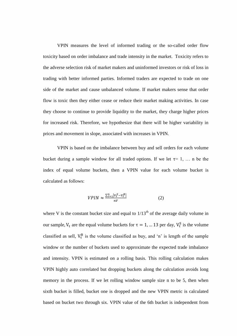
VPIN measures the level of informed trading or the so-called order flow

toxicity based on order imbalance and trade intensity in the market. Toxicity refers to

the adverse selection risk of market makers and uninformed investors or risk of loss in

trading with better informed parties. Informed traders are expected to trade on one

side of the market and cause unbalanced volume. If market makers sense that order

flow is toxic then they either cease or reduce their market making activities. In case

they choose to continue to provide liquidity to the market, they charge higher prices

for increased risk. Therefore, we hypothesize that there will be higher variability in

prices and movement in slope, associated with increases in VPIN.

VPIN is based on the imbalance between buy and sell orders for each volume

bucket during a sample window for all traded options. If we let = 1, … n be the

index of equal volume buckets, then a VPIN value for each volume bucket is

calculated as follows:

∑ |

|

(2)

where V is the constant bucket size and equal to 1/13th

of the average daily volume in

our sample are the equal volume buckets for per day, is the volume

classified as sell, is the volume classified as buy, and ‘n’ is length of the sample

window or the number of buckets used to approximate the expected trade imbalance

and intensity. VPIN is estimated on a rolling basis. This rolling calculation makes

VPIN highly auto correlated but dropping buckets along the calculation avoids long

memory in the process. If we let rolling window sample size n to be 5, then when

sixth bucket is filled, bucket one is dropped and the new VPIN metric is calculated

based on bucket two through six. VPIN value of the 6th bucket is independent from

the VPIN value of the first bucket. If we let n to be 13, then this is equivalent to

calculating a daily VPIN. Since we are working with high frequency data we want

VPIN metric to be updated intraday and we use n as 5. We have an average of 13

VPIN values per day but on very active days the VPIN metric is updated much more

frequently than on less active days.

VPIN has two advantages compared to PIN measure (Easley et al., 1996)

which has been widely used in the literature as a proxy for the level of informed

trading in markets. First, we do not have to estimate unobserved parameters for VPIN.

Second, there are also criticisms against PIN for being a proxy for only illiquidity

effects and not asymmetric information. (Duarte and Young, 2009; Akay et al., 2012).

VPIN is less prone to infrequent trading since equal volume buckets are used. Table

IV presents the summary statistics for our variables in volume time. Average VPIN is

0.38 with a maximum of 1 and a minimum of 0.04. Average implied volatility is 10%

for calls and 17% for puts. Average VIX is 13.09% annually.

……Insert Table IV about here…..

3. Empirical Results

The objective of this section is to explore the linkage between the variables

discussed in the prior section and changes in slope of implied volatility skew of S&P

500 options. We start the analysis by conducting the Augmented Dickey-Fuller

stationarity tests on our variables. We are able to reject the existence of a unit root for

all of our variables and first difference of VIX. Observation of the ACF reveals that

change in slope is highly auto-correlated and we include first lag of slope as an

independent variable in the regression.

To assess the relation between slope and variables discussed above, we

estimate the following regression with Newey-West corrected standard errors:

(3)

where ΔSlopen is change in one of the two measures of slope defined in Equation (1)

from volume bar n-1 to n. Rn is the index return computed from volume bar n-13 to n-

1 for the momentum effect. Timen is option’s annualized time to maturity. Spreadn is

the relative bid-ask spread, namely bid-ask spread divided by an option’s mid quote

and is calculated for calls and puts separately for each moneyness category. RVn is

realized volatility which is the sum of squared five-min returns during each day. NBPn

is the net buying pressure calculated as the difference between buyer motivated and

seller motivated trades times the absolute value of delta for each moneyness category

of calls and puts separately. NBP variables vary in different regressions depending on

the slope measure. VPINn is the metric for probability of informed trading and

calculated as in Equation (2).

Table V displays the results of regression in Equation (3) and show that all of

our variables except momentum seem to contribute to the variability of slope of

implied volatility skew of S&P 500 Index Options. Pena et al. finds a weak relation

between market momentum and degree of curvature of the smile and in our analysis

the effect of momentum on slope is not significant. In line with Pena et al.’s (1999)

findings for Spanish Index options we find that change in slope of S&P 500 Index

options is related to transactions costs represented by bid-ask spreads and option time

to maturity. The lagged change in slope is negatively and significantly related to

current change in both measures of slope. This is in line with limits to arbitrage

theorem which suggests that as market makers rebalance their portfolios, prices

reverse to their previous levels gradually.

In line with Bollen and Whaley (2004), NBP of options significantly affect

slope. NBP of ATM calls seem to be negatively associated with both measures of

slope. NBP of ATM (OTM) puts is significantly and positively associated with Slope1

(Slope2). Besides these variables, we find a significant relation between VPIN and

slope. The relation is positive for both measures of slope. This implies that the higher

the level of private information and order flow toxicity in the market, the more

asymmetrically the OTM and ATM puts are valued in the market relative to ATM

calls.

……Insert Table V about here…..

Informed traders try to time their trades at times of high level of trading and

liquidity and macroeconomic announcements provide an avenue for investors to trade

more aggressively on their private information. If VPIN captures the probability of

informed trading well, then it would be interesting to see the relation between VPIN

and slope at macroeconomic announcement times. The macroeconomic

announcement timings, realizations and survey expectations are obtained from

Bloomberg. Table VI lists the macroeconomic announcements that we include in our

analysis. We include 23 macroeconomic announcements and most of the

announcements are monthly but initial jobless claims announcement is weekly and we

also have a number of quarterly announcements.

……Insert Table VI about here…..

We first visually examine behavior of slope and VPIN around macroeconomic

announcements. We calculate the averages of slope and VPIN for each volume bar

corresponding to the announcement time t, and up to 15 pre-announcement and post-

announcement volume bars from January through December in 2006. Figures 3 and 4

plot these averages. Figure 3 shows that Slope2 drops sharply in response to an

announcement release but drop is not that significant for Slope1. In Figure 4, we

observe that VPIN calculated over a window size of 5, starts to decrease 5 volume

bars before the announcement and increases afterwards. Before the announcement, we

observe a tranquil period for informed traders in options market, which could be due

to investors’ tendency to wait for the releases and postpone their trades. Informed

trading activity increases within nine volume bars following an announcement. As

most of the announcements coincide with market opening, it is difficult to anticipate

the response time of the informed traders to the announcement release, nine volume

bars might correspond to a very short period of response time.

……Insert Figure 3 and 4 about here…..

We continue our analysis with adding one more variable to the regression

equation (3) to test the relation between VPIN and implied volatility skew at

macroeconomic announcements times. This variable is the News dummy which is 1 if

there is a macroeconomic announcement and 0 otherwise. Table VII summarizes the

results. When we account for macroeconomic announcements, the effect of VPIN is

less significant for both Slope1 and Slope2. We observe a strong negative impact of

News dummy on Slope2. This suggests that the effect of uncertainty resolution

dominates when there is a macroeconomic announcement and OTM puts are valued

more symmetrically in the market relative to ATM calls. This is also observed in

Figure 3 as a sharp drop in Slope2.

……Insert Table VII about here…..

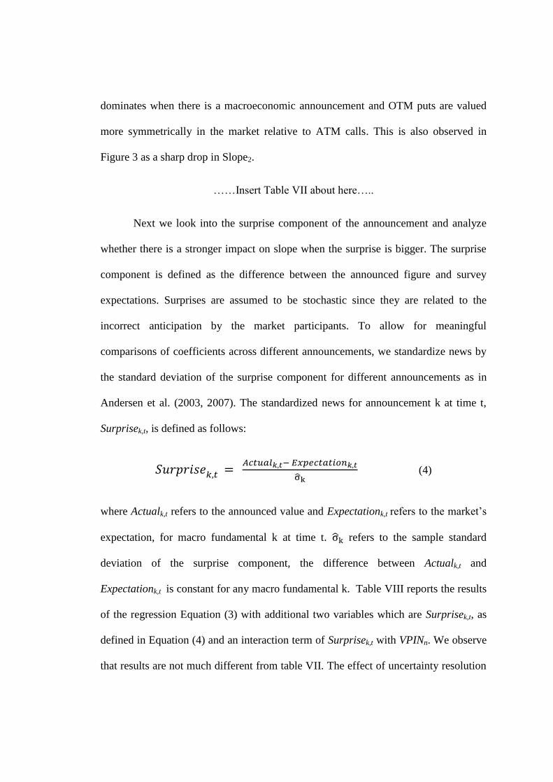
Next we look into the surprise component of the announcement and analyze

whether there is a stronger impact on slope when the surprise is bigger. The surprise

component is defined as the difference between the announced figure and survey

expectations. Surprises are assumed to be stochastic since they are related to the

incorrect anticipation by the market participants. To allow for meaningful

comparisons of coefficients across different announcements, we standardize news by

the standard deviation of the surprise component for different announcements as in

Andersen et al. (2003, 2007). The standardized news for announcement k at time t,

Surprisek,t, is defined as follows:

(4)

where Actualk,t refers to the announced value and Expectationk,t refers to the market’s

expectation, for macro fundamental k at time t. refers to the sample standard

deviation of the surprise component, the difference between Actualk,t and

Expectationk,t is constant for any macro fundamental k. Table VIII reports the results

of the regression Equation (3) with additional two variables which are Surprisek,t, as

defined in Equation (4) and an interaction term of Surprisek,t with VPINn. We observe

that results are not much different from table VII. The effect of uncertainty resolution

is still there for Slope2 and the impact of the macroeconomic surprises are not higher

than the impact of macroeconomic announcement dummy variable.

……Insert Table VIII about here…..

4. Risk Neutral Skewness and VPIN

In this section we further investigate whether order flow toxicity measured by

VPIN metric is associated with risk aversion. As a proxy for risk aversion, we use

risk-neutral skewness measure of Bakshi et al. (2003). The beauty of this measure is

that it is model-free and relies on the basic result that any payoff can be replicated and

priced using options with different strikes (Bakshi and Madan, 2000). Bakshi et al.

(2003) show that the more negative the risk-neutral skew, the steeper the volatility

smile is. In this respect, we expect variability of VPIN to be associated with higher

variability in risk-neutral skewness as well.

Risk neutral skewness and kurtosis are recovered using market prices of OTM

calls and puts as follows:

( ) ( ) ( ) ( ) ( )

( ) ( ) (5)

( )= ( ) ( ) ( ) ( ) ( ) ( )

( ) ( )

Where ( ) and ( ) are the prices of index calls and puts with strike price,

K, and expiration periods from time t. ( ) and the prices of quadratic, cubic and

quartic contracts are as follows:

( ) =

( )

( )

( ) (6)

( ) ∫ ( (

( )

))

( )

( )

∫ ( (

( )

))

( )

( )

( ) ∫ (

( )

) (

( ))

( )

( )

∫ (

( )

) (

( ))

( )

( )

( ) ∫ (

( )

)

(

( ))

( )

( )

∫ (

( )

)

(

( ))

( )

( )

We use trapezoid estimations to calculate the above integrals as in Dennis and

Mayhew (2002) and Conrad et al. (2013) and estimate moments for each volume

bucket in our sample.

We then investigate whether VPIN is associated with risk neutral skews using

our prior ordinary least squares regression using change in skewness as the dependent

variable and including kurtosis as an additional control variable.

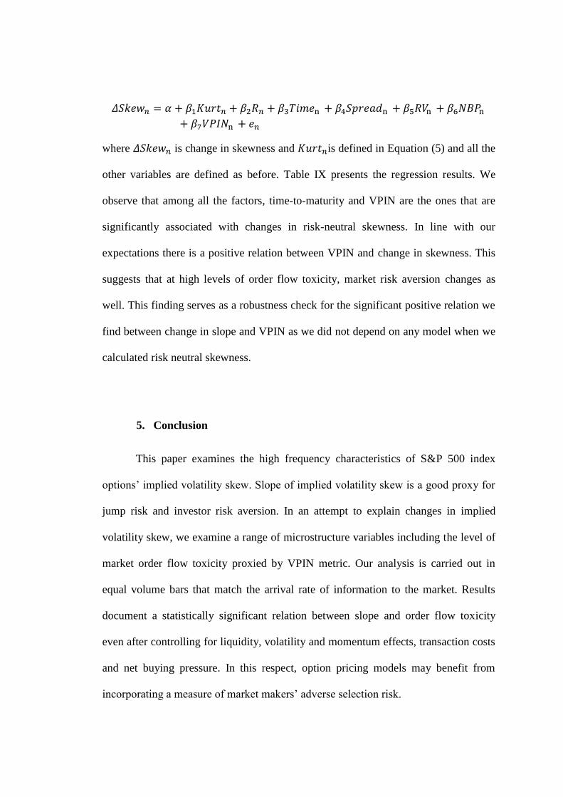
where is change in skewness and is defined in Equation (5) and all the

other variables are defined as before. Table IX presents the regression results. We

observe that among all the factors, time-to-maturity and VPIN are the ones that are

significantly associated with changes in risk-neutral skewness. In line with our

expectations there is a positive relation between VPIN and change in skewness. This

suggests that at high levels of order flow toxicity, market risk aversion changes as

well. This finding serves as a robustness check for the significant positive relation we

find between change in slope and VPIN as we did not depend on any model when we

calculated risk neutral skewness.

5. Conclusion

This paper examines the high frequency characteristics of S&P 500 index

options’ implied volatility skew. Slope of implied volatility skew is a good proxy for

jump risk and investor risk aversion. In an attempt to explain changes in implied

volatility skew, we examine a range of microstructure variables including the level of

market order flow toxicity proxied by VPIN metric. Our analysis is carried out in

equal volume bars that match the arrival rate of information to the market. Results

document a statistically significant relation between slope and order flow toxicity

even after controlling for liquidity, volatility and momentum effects, transaction costs

and net buying pressure. In this respect, option pricing models may benefit from

incorporating a measure of market makers’ adverse selection risk.

We further analyze the relation between VPIN and slope at macroeconomic

announcement times. Informed traders try to time their trades at times of high level of

trading and liquidity and macroeconomic announcements provide an avenue for

investors to trade more aggressively on their private information. We find that when

there is a macroeconomic announcement, the association between VPIN and both

measures of slope is weaker. When there is a macroeconomic announcement, the

effect of uncertainty resolution seems to dominate and OTM puts are valued more

symmetrically in the market relative to ATM calls.

Finally we investigate whether order flow toxicity measured by VPIN metric

is associated with risk-neutral skewness which is highly correlated with slope. Risk

neutral skewness measure of Bakshi et al. (2003) is model-free and uses prices of

options with different strikes. We expect to see a significant relation between risk

neutral skewness and VPIN. In line with our expectations, we observe that order flow

toxicity and level of private information is significantly associated with investor risk

aversion proxied by risk-neutral skewness. A clearer comprehension about the factors

that affect the slope and risk-neutral skewness is important for developing new option

pricing models and devising proper hedging and investment strategies. Our results

justify why traders shall closely monitor slope and skewness to understand how jump

risk and risk aversion are evolving during a trading day.

Acknowledgements

We would like to acknowledge financial support from the Scientific and

Technological Research Council of Turkey (TUBITAK).

References

Admati, A. R., & Pfleiderer, P., 1988. A theory of intraday patterns: Volume and

price variability. Review of Financial Studies, 1(1), 3-40.

Akay, O. O., Cyree, K. B., Griffiths, M. D., Winters, D. B., 2012. What does PIN

identify? Evidence from the T-bill market. Journal of Financial Markets, 15(1), 29-46.

Amihud, Y., Mendelson, H., 1986. Asset pricing and the bid-ask spread. Journal of

financial Economics, 17(2), 223-249.

Amin, K., Coval, J. D., Seyhun, H. N., 2004. Index Option Prices and Stock Market

Momentum*. The Journal of Business, 77(4), 835-874.

Andersen, T., Bollerslev, T., Diebold, F. X., Labys, P., 2001. “The Distribution of

Realized Stock Return Volatility,” Journal of Financial Economics, 61, 43-76.

Andersen, T., Bollerslev, T., Diebold, F. 2003a. Some like it smooth, and some like it

rough: untangling continuous and jump components in measuring, modeling, and

forecasting asset return volatility.

Andersen, T.G., Bollerslev, T., Diebold, F.X., Vega, C., 2003b. “Micro Effects of

Macro Announcements: Real-Time Price Discovery in Foreign Exchange,” American

Economic Review, 93, 38-62.

Andersen, T. G., Bollerslev, T., Diebold, F. X., 2007a. Roughing it up: Including

jump components in the measurement, modeling, and forecasting of return volatility.

The Review of Economics and Statistics, 89(4), 701-720.

Andersen, T. G., Bollerslev, T., Diebold, F. X., Vega, C., 2007b. Real-time price

discovery in global stock, bond and foreign exchange markets. Journal of

International Economics, 73(2), 251-277.

Bakshi, G., Madan, D., 2000. Spanning and derivative-security valuation. Journal of

Financial Economics, 55(2), 205-238.

Bakshi, G., Kapadia, N., Madan, D., 2003. Stock return characteristics, skew laws,

and the differential pricing of individual equity options. Review of Financial Studies,

16(1), 101-143.

Bates, D. S., 1996. Jumps and stochastic volatility: Exchange rate processes implicit

in Deutsche Mark options. Review of financial studies, 9(1), 69-107.

Bernile, G., Hu, J., Tang, Y., 2014. Can information be locked-up? Informed trading

ahead of macro-news announcements. Informed Trading Ahead of Macro-News

Announcements.

Bollen, N. P., Whaley, R. E., 2004. Does net buying pressure affect the shape of

implied volatility functions? The Journal of Finance, 59(2), 711-753.

Buraschi, A., Jiltsov, A., 2006. Model uncertainty and option markets with

heterogeneous beliefs. The Journal of Finance, 61(6), 2841-2897.

Cetin, U., Jarrow, R., Protter, P., Warachka, M., 2006. Pricing options in an extended

Black Scholes economy with illiquidity: Theory and empirical evidence. Review of

Financial Studies, 19(2), 493-529.

Chou, R. K., Chung, S. L., Hsiao, Y. J., Wang, Y. H., 2011. The impact of liquidity

on option prices. Journal of Futures Markets, 31(12), 1116-1141.

Conrad, J., Dittmar, R. F., Ghysels, E., 2013. Ex ante skewness and expected stock

returns. The Journal of Finance, 68(1), 85-124.

Cremers, M., Driessen, J., Maenhout, P., Weinbaum, D., 2008. Individual stock-

option prices and credit spreads. Journal of Banking & Finance, 32(12), 2706-2715.

Cremers, M., & Weinbaum, D., 2010. Deviations from put-call parity and stock return

predictability. Journal of Financial and Quantitative Analysis, 45(2), 335.

Dennis, P., & Mayhew, S., 2002. Risk-neutral skewness: Evidence from stock

options. Journal of Financial and Quantitative Analysis, 37(03), 471-493.

Deuskar, P., Gupta, A., Subrahmanyam, M. G., 2008. The economic determinants of

interest rate option smiles. Journal of Banking & Finance, 32(5), 714-728.

Deuskar, P., Gupta, A., Subrahmanyam, M. G., 2011. Liquidity effect in OTC options

markets: Premium or discount? Journal of Financial Markets, 14(1), 127-160.

Duan, J. C., Wei, J., 2009. Systematic risk and the price structure of individual equity

options. Review of Financial Studies, 22(5), 1981-2006.

Duarte, J., Young, L., 2009. Why is< i> PIN</i> priced?. Journal of Financial

Economics, 91(2), 119-138.

Dumas, B., Fleming, J., Whaley, R. E., 1998. Implied volatility functions: Empirical

tests. The Journal of Finance, 53(6), 2059-2106.

Easley, D. and M. O’Hara, 1992. Time and the process of security price adjustment.

The Journal of finance, 47(2), 577-605.

Easley, D., Kiefer, N. M., O'hara, M., Paperman, J. B., 1996. Liquidity, information,

and infrequently traded stocks. The Journal of Finance, 51(4), 1405-1436.

Easley, D., de Prado, M. M. L., O'Hara, M., 2012. Flow toxicity and liquidity in a

high-frequency world. Review of Financial Studies, 25(5), 1457-1493.

Ederington, L. H., Lee, J. H., 1996. The creation and resolution of market uncertainty:

the impact of information releases on implied volatility. Journal of Financial and

Quantitative Analysis, 31(4).

Ederington, L. H., Guan, W., 2002. Why are those options smiling?. The Journal of

Derivatives, 10(2), 9-34.

Feng, S. P., Hung, M. W., Wang, Y. H., 2014. Option pricing with stochastic liquidity

risk: Theory and evidence. Journal of Financial Markets, 18, 77-95.

Garleanu, N., Pedersen, L. H., Poteshman, A. M., 2009. Demand-based option

pricing. Review of Financial Studies, 22(10), 4259-4299.

Gençay, R., Dacorogna, M., Muller, U. A., Pictet, O., Olsen, R., 2001. An

introduction to high-frequency finance. Access Online via Elsevier.

Green, T. C., 2004. Economic news and the impact of trading on bond prices. The

Journal of Finance, 59(3), 1201-1234.

Han, B., 2008.. Investor sentiment and option prices. Review of Financial Studies,

21(1), 387-414.Hasbrouck, Joel. "The summary informativeness of stock trades: An

econometric analysis." Review of Financial Studies 4.3 (1991): 571-595.

Heston, S. L., 1993. A closed-form solution for options with stochastic volatility with

applications to bond and currency options. Review of financial studies, 6(2), 327-343.

Hull, J., 1993. Options, Futures, and Other Derivative Securities. Prentice-Hall, Inc,

Englewood Cliffs, NJ (1993)

Kandel, E., Pearson, N. D., 1995. Differential interpretation of public signals and

trade in speculative markets. Journal of Political Economy, 831-872.

Kearney, A. A., Lombra, R. E., 2004. Stock market volatility, the news, and monetary

policy. Journal of economics and finance, 28(2), 252-259.

Kim, J. B., Zhang, L., 2010. Financial Reporting Opacity and Expected Crash Risk:

Evidence from Implied Volatility Smirks. Available at SSRN 1649182.

Lee, C., & Ready, M. J. 1991. Inferring trade direction from intraday data. The

Journal of Finance, 46(2), 733-746.

Longstaff, F. A., 1995. Option pricing and the martingale restriction. Review of

Financial Studies, 8(4), 1091-1124.

MacBeth, J. D., Merville, L. J., 1979. An Empirical Examination of the Black‐Scholes

Call Option Pricing Model. The Journal of Finance, 34(5), 1173-1186.

Nordén, L., Xu, C., 2012. Option happiness and liquidity: Is the dynamics of the

volatility smirk affected by relative option liquidity?. Journal of Futures Markets,

32(1), 47-74.

Onan, M., Salih, A., Yasar, B., 2014. Impact of Macroeconomic Announcements on

Implied Volatility Slope of SPX Options and VIX. Finance Research Letters.

Pasquariello, P.,Vega, C., 2007. Informed and strategic order flow in the bond

markets. Review of Financial Studies, 20(6), 1975-2019.

Pena, I., Rubio, G., Serna, G., 1999. Why do we smile? On the determinants of the

implied volatility function. Journal of Banking & Finance, 23(8), 1151-1179.

Rubinstein, M., 1985. Nonparametric tests of alternative option pricing models using

all reported trades and quotes on the 30 most active CBOE option classes from

August 23, 1976 through August 31, 1978. The Journal of Finance, 40(2), 455-480.

Santa-Clara, P., Yan, S., 2010. Crashes, volatility, and the equity premium: Lessons

from S&P 500 options. The Review of Economics and Statistics, 92(2), 435-451.

Toft, K. B., Prucyk, B., 1997. Options on leveraged equity: Theory and empirical

tests. The Journal of Finance, 52(3), 1151-1180.

Xing, Y., Zhang, X., Zhao, R., 2010. What does the individual option volatility smirk

tell us about future equity returns? Journal of Financial and Quantitative Analysis,

45(3), 641.

Yan, S., 2011. Jump risk, stock returns, and slope of implied volatility smile. Journal

of Financial Economics, 99(1), 216-233.

Figure 1: Intraday behavior of S&P 500 trading Figure shows the

intraday (thirty-min) behavior of average number of contracts and average

dollar volume for SPX thirty-day options for a total observations of 585,991

during 2006.

60000

80000

100000

120000

140000

160000

5000

10000

15000

20000

25000

30000

Average Number of Contracts

Average Volume

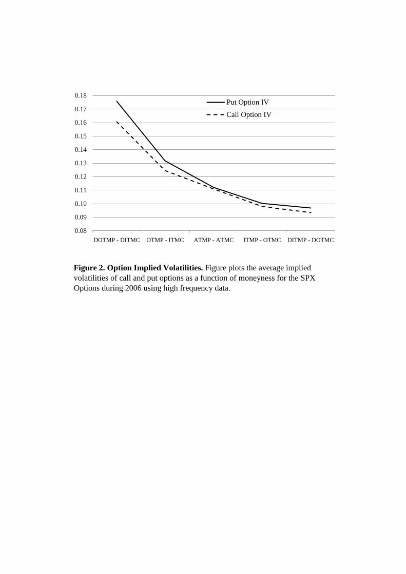
Figure 2. Option Implied Volatilities. Figure plots the average implied

volatilities of call and put options as a function of moneyness for the SPX

Options during 2006 using high frequency data.

0.08

0.09

0.10

0.11

0.12

0.13

0.14

0.15

0.16

0.17

0.18

DOTMP - DITMC OTMP - ITMC ATMP - ATMC ITMP - OTMC DITMP - DOTMC

Put Option IV

Call Option IV

Figure 3. Behavior of Slope at Announcements in Volume Time. Figure

plots the average of slope for each volume bucket corresponding to the

announcement time t during 2006. Pre-announcement and post-announcement

means of slope are also included up to 15 volume buckets

0.0002

0.0004

0.0006

0.0008

0.0010

0.0012

0.0014

0.0016

t -

15

t -

13

t -

11

t -

9

t -

7

t -

5

t -

3

t -

1

t +

1

t +

3

t +

5

t +

7

t +

9

t +

11

t +

13

t +

15

Slope1

0.0186

0.0190

0.0194

0.0198

0.0202

t -

15

t -

13

t -

11

t -

9

t -

7

t -

5

t -

3

t -

1

t +

1

t +

3

t +

5

t +

7

t +

9

t +

11

t +

13

t +

15

Slope2

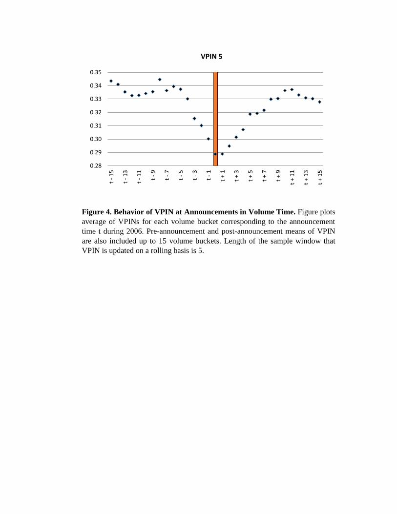
Figure 4. Behavior of VPIN at Announcements in Volume Time. Figure plots

average of VPINs for each volume bucket corresponding to the announcement

time t during 2006. Pre-announcement and post-announcement means of VPIN

are also included up to 15 volume buckets. Length of the sample window that

VPIN is updated on a rolling basis is 5.

0.28

0.29

0.30

0.31

0.32

0.33

0.34

0.35

t -

15

t -

13

t -

11

t -

9

t -

7

t -

5

t -

3

t -

1

t +

1

t +

3

t +

5

t +

7

t +

9

t +

11

t +

13

t +

15

VPIN 5

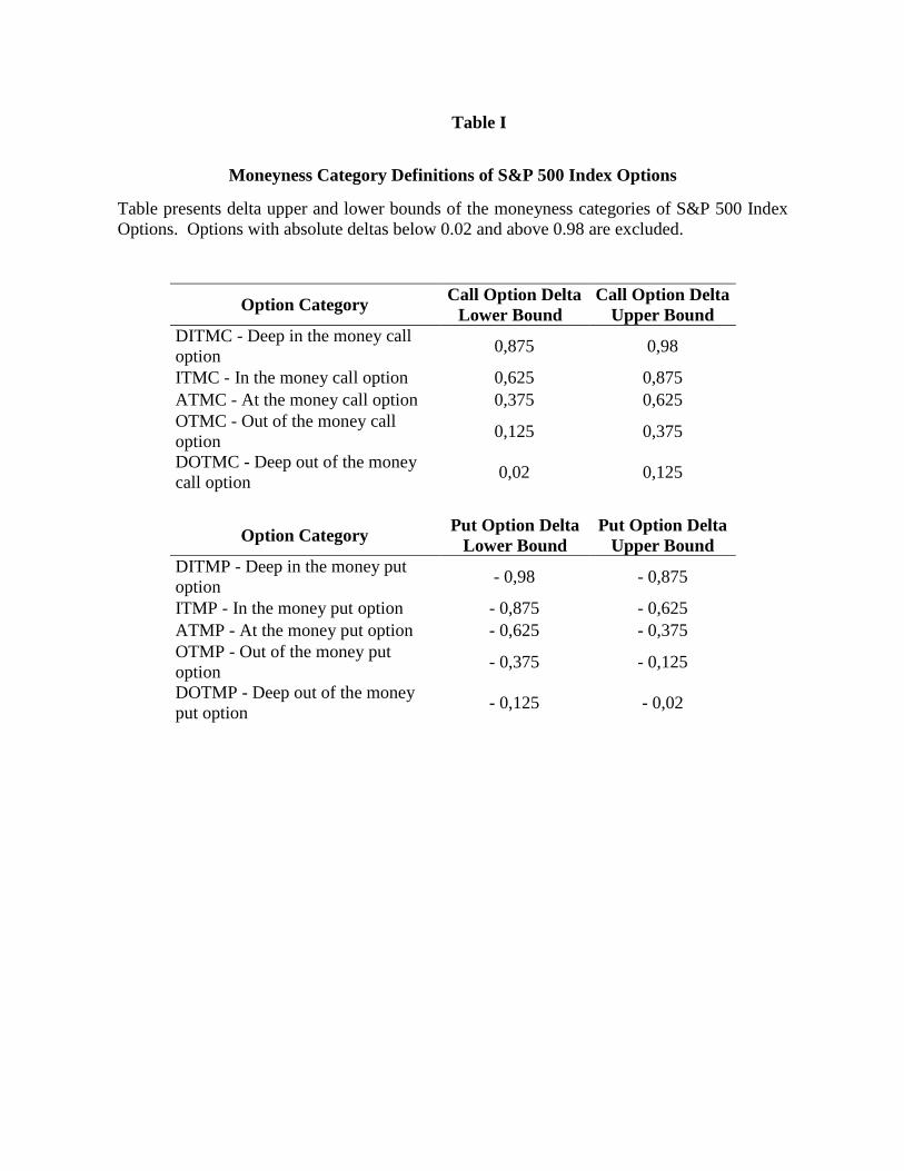
Table I

Moneyness Category Definitions of S&P 500 Index Options

Table presents delta upper and lower bounds of the moneyness categories of S&P 500 Index

Options. Options with absolute deltas below 0.02 and above 0.98 are excluded.

Option Category Call Option Delta

Lower Bound

Call Option Delta

Upper Bound

DITMC - Deep in the money call

option 0,875 0,98

ITMC - In the money call option 0,625 0,875

ATMC - At the money call option 0,375 0,625

OTMC - Out of the money call

option 0,125 0,375

DOTMC - Deep out of the money

call option 0,02 0,125

Option Category Put Option Delta

Lower Bound

Put Option Delta

Upper Bound

DITMP - Deep in the money put

option - 0,98 - 0,875

ITMP - In the money put option - 0,875 - 0,625

ATMP - At the money put option - 0,625 - 0,375

OTMP - Out of the money put

option - 0,375 - 0,125

DOTMP - Deep out of the money

put option - 0,125 - 0,02

Table II

Distribution of Buyer/Seller Motivated S&P 500 Index Option Trades

Table presents the distribution of buyer/seller motivated S&P 500 Index options traded on

Chicago Board Options Exchange in 2006 subject to filtration discussed in section 2.1. We use Lee and Ready (1991) algorithm to classify trades. According to this algorithm, transactions that

occur at prices higher (lower) than the quote midpoint are classified as buyer-initiated (seller-

initiated). Transactions that occur at a price that equals the quote midpoint but is higher (lower)

than the previous transaction price are classified as buyer-initiated (seller-initiated). Transactions

that occur at a price that equals both the quote midpoint and the previous transaction price but is

higher (lower) than the last different transaction price are classified as being buyer-initiated

(seller-initiated). We discard unidentified trades which constitute 1.3% of the population.

Identification Type Number of Trades Prop. of Total

Buy 256,332 53.2%

Sell 219,081 45.5%

Unidentified 6,317 1.3%

Total 481,730 100.0%

Table III

Summary of Net Buying Pressure for S&P 500 Index Options

Table presents the distribution of buyer/seller motivated S&P 500 Index options, traded on

Chicago Board Options Exchange in 2006 subject to filtration discussed in section 2.1, according

to moneyness categories. Moneyness category definitions are as in Table I. Net is the difference between buyer and seller motivated trades.

Category Buy Sell Net Total

Prop. of

Total (%)

CALLS

DITMC 195,785 114,15 81,635 309,935 0.7

ITMC 543,831 543,418 413 1,087,249 2.5

ATMC 2,446,186 2,249,534 196,652 4,695,720 10.9

OTMC 2,010,184 1,632,883 377,301 3,643,067 8.5

DOTMC 2,576,943 2,593,281 -16,338 5,170,224 12.0

TOTAL 7,772,929 7,133,266 639,663 14,906,195 34.7

PUTS

DITMP 48,866 15,012 33,854 63,878 0.1

ITMP 167,299 213,136 -45,837 380,435 0.9

ATMP 2,383,708 2,229,217 154,491 4,612,925 10.7

OTMP 3,899,926 3,492,139 407,787 7,392,065 17.2

DOTMP 7,782,305 7,810,069 -27,764 15,592,374 36.3

TOTAL 14,282,104 13,759,573 522,531 28,041,677 65.3

ALL

22,055,033 20,892,839 1,162,194 42,947,872 100.0

Table IV

Summary Statistics

Table lists the summary statistics for our variables. VPIN is the order flow toxicity metric

calculated as in Equation (2). Calls NBP (Puts NBP) is the net buying pressure calculated as the

difference between buyer motivated and seller motivated trades. Calls Imp. Volatility (Puts Imp.

Volatility) is the average of implied volatilities for calls (puts). Calls Spread (Puts Spread) is the

relative bid-ask spread, namely bid-ask spread divided by an option’s mid quote for calls (puts).

Slope is one of the two measures of slope defined in Equation (1). Index is index level. Index

Return is the index return computed from volume bar n-13 to n-1. Real. Volatility is realized

volatility which is the sum of squared five-min returns during each day. VIX is the CBOE’s

volatility index for the S&P 500 index return.

Variable Name Min Median Max Mean Std. Dev. Skewness Kurtosis

VPIN 0.04 0.34 1.00 0.38 0.19 0.80 3.21 Calls NBP -5678.46 15.17 16311.92 81.25 1201.35 2.01 26.36 Calls Imp. Volatility 0.07 0.10 0.18 0.10 0.02 0.93 3.51 Calls Spread 0.03 0.15 1.43 0.17 0.09 3.97 34.09 Puts NBP -32395.32 45.15 6989.40 45.71 1224.09 -9.22 230.07 Puts Imp. Volatility 0.09 0.13 0.27 0.14 0.03 1.06 3.69 Puts Spread 0.04 0.13 0.68 0.14 0.06 3.02 16.45 ATM Calls NBP -4128.43 0.54 9320.21 26.62 685.71 0.99 19.47 ATM Calls Spread 0.01 0.07 0.32 0.07 0.02 1.69 12.86 ATM Puts NBP -32396.52 1.22 4725.65 16.15 998.57 -17.22 517.47 ATM Puts Spread 0.01 0.07 0.22 0.07 0.02 0.92 6.92 OTM Puts NBP -3088.33 2.46 3232.77 35.80 478.48 0.16 9.20 OTM Puts Spread 0.02 0.10 0.31 0.11 0.03 1.09 7.10 DOTM Puts NBP -2164.55 0.00 2373.45 -5.13 253.32 -0.42 14.36 DOTM Puts Spread 0.03 0.22 1.06 0.23 0.09 2.08 10.96 Slope1 -0.07 0.00 0.04 0.00 0.01 -2.11 26.78 Slope2 -0.05 0.02 0.09 0.02 0.01 0.87 5.43 Index 1219.73 1295.20 1431.59 1308.75 52.32 0.82 2.56 Index Return -0.02 0.00 0.03 0.00 0.01 0.09 4.71 Real. Volatility 0.00 0.08 0.43 0.09 0.05 2.75 13.41 VIX 9.44 12.07 22.99 13.09 2.58 1.10 3.63

Table V

Determinants of Slope of S&P 500 Index Options Skew

Table presents the regression results of

where ΔSlopen is change in one of the two

measures of slope defined in Equation (1) from volume bar n-1 to n. Rn is the index return

computed from volume bar n-13 to n-1for the momentum effect. Spreadn is the relative bid-ask

spread, namely bid-ask spread divided by an option’s mid quote and RVn is realized volatility which is the sum of squared five-min returns during each day. Timen is option’s annualized time

to maturity. NBPn is the net buying pressure calculated as the difference between buyer

motivated and seller motivated trades times the absolute value of delta for each moneyness

category. VPINn is the metric for probability of informed trading and calculated as in Equation

(2). ***, **,* denote statistical significance at the 1%, 5% and 10% levels respectively.

Δ Slope1

Δ Slope2

Coefficient t-value

Coefficient t-value

Intercept -0.003 -3.334 *** -0.006 -5.751 ***

Δslopen-1 -0.346 -20.466 *** -0.379 -22.569 ***

R 0.025 1.465

0.002 0.091

Time 0.005 0.915

0.016 2.513 **

Atm Call Spread 0.004 0.888

-0.007 -1.118

Atm Put Spread 0.016 2.860 ***

Otm Put Spread

0.040 8.927 ***

RV 0.004 1.900 * 0.002 0.617

Atm Call NBP -0.014 -7.476 *** -0.010 -4.442 ***

Atm Put NBP 0.015 7.787 ***

Otm Put NBP

0.014 4.205 ***

VPIN 0.001 2.575 *** 0.002 2.438 **

Table VI

Macroeconomic Announcements

Table lists the macroeconomic announcements used in this study along with the category, timing

in EST, source, frequency. Abbreviations are Investors Business Daily (IBD), Automatic Data

Processing (ADP), Federal Reserve Board (FRB), Bureau of Labor and Statistics (BLS), Bureau

of Economic Analysis (BEA), Bureau of the Census (BC), Conference Board (CB), US.

Department of Labor (UDL), Institute for Supply Management (ISM), Federal Reserve Bank of

Philadelphia (FRBP) and National Association of Realtors (NAR).

Macroeconomic Announcement Time Source Frequency

ADP Employment Change 8:15 ADP Five times

Unemployment Rate 8:30 BLS Monthly

Initial Jobless Claims 8:30 UDL Weekly

Consumer Price Index 8:30 BLS Monthly

Unit Labor Costs 8:30 BLS Eight times

GDP Price Index 8:30 BEA Monthly

Producer Price Index 8:30 BLS Monthly

Chicago Purchasing Manager 10:00 ISM Monthly

Consumer Confidence 10:00 CB Monthly

IBD/TIPP Economic Optimism 10:00 IBD Six times

Philadelphia Fed. 12:00 FRBP Monthly

Index of Leading Indicators 10:00 CB Monthly

Housing Starts 8:30 BC Monthly

Durable Goods Orders* 8:30 BC Monthly

Factory Orders 10:00 BC Monthly

Construction Spending 10:00 BC Monthly

Business Inventories 10:00 BC Monthly

Wholesale Inventories 10:00 BC Monthly

Personal Income/Spending 8:30 BEA Monthly

Retail Sales Less Autos 8:30 BC Monthly

Capacity Utilization/Industrial Production 9:15 FRB Monthly

Existing Home Sales 8:30 NAR Monthly

New Home Sales 10:00 BC Monthly

*When there is also a GDP announcement that day, the durable goods orders announcement is

made at 10:00 AM

Table VII

VPIN and Slope at Macroeconomic Announcement Times

Table presents the regression results of

( )

where ΔSlopen is change in one of the two measures of slope defined in Equation (1) from

volume bar n-1 to n. Rn is the index return computed from volume bar n-13 to n-1for the

momentum effect. Spreadn is the relative bid-ask spread, namely bid-ask spread divided by an

option’s mid quote and RVn is realized volatility which is the sum of squared five-min returns

during each day. Timen is option’s annualized time to maturity. NBPn is the net buying pressure

calculated as the difference between buyer motivated and seller motivated trades times the

absolute value of delta for each moneyness category. VPINn is the metric for probability of

informed trading and calculated as in Equation (2). Newsn is a dummy variable that takes one for

the volume bucket n that includes a macroeconomic announcement and zero otherwise ***, **,*

denote statistical significance at the 1%, 5% and 10% levels respectively.

Δ Slope1

Δ Slope2

Coefficient t-value

Coefficient t-value

Intercept -0.003 -3.223 *** -0.006 -5.515 ***

Δslopen-1 -0.345 -20.414 *** -0.379 -22.597 ***

R 0.025 1.485

0.004 0.167

Time 0.005 0.908

0.016 2.510 **

Atm Call

Spread 0.005 0.897

-0.007 -1.113

Atm Put Spread 0.016 2.872 ***

Otm Put Spread

0.040 9.053 ***

RV 0.004 1.897 * 0.001 0.588

Atm Call NBP -0.014 -7.476 *** -0.010 -4.444 ***

Atm Put NBP 0.015 7.789 ***

Otm Put NBP

0.014 4.273 ***

VPIN 0.001 2.290 ** 0.001 1.745 *

News -0.001 -0.677

-0.003 -2.268 **

News*VPIN 0.000 0.138

0.004 1.145

Table VIII

VPIN and Slope with Macroeconomic Announcement Surprises

Table presents the regression results of

(

) where ΔSlopen is change in change in one of the two measures of slope defined in

Equation (1) from volume bar n-1 to n. Rn is the index return computed from volume bar n-13 to

n-1for the momentum effect. Spreadn is the relative bid-ask spread, namely bid-ask spread

divided by an option’s mid quote and RVn is realized volatility which is the sum of squared five-

min returns during each day. Timen is option’s annualized time to maturity. NBPn is the net

buying pressure calculated as the difference between buyer motivated and seller motivated trades

times the absolute value of delta standardized by volume for each moneyness category. VPINn is

the metric for probability of informed trading and calculated as in Equation (2). is

defined as in Equation (4). ***, **,* denote statistical significance at the 1%, 5% and 10% levels

respectively.

Δ Slope1

Δ Slope2

Coefficient t-value

Coefficient t-value

Intercept -0.003 -3.190 *** -0.006 -5.573 ***

Δslopen-1 -0.345 -20.348 *** -0.379 -22.487 ***

R 0.028 1.630

0.004 0.175

Time 0.005 0.914

0.017 2.538 **

Atm Call

Spread 0.005 0.942

-0.007 -1.057

Atm Put

Spread 0.016 2.902 ***

Otm Put Spread

0.040 9.067 ***

RV 0.003 1.777 * 0.001 0.455

Atm Call NBP -0.014 -7.355 *** -0.011 -4.566 ***

Atm Put NBP 0.015 7.800 ***

Otm Put NBP

0.014 4.146 ***

VPIN 0.001 2.201 ** 0.001 1.855 *

Surprise -0.001 -1.562

-0.002 -2.467 **

Surprise*VPIN 0.001 0.687

0.003 1.297

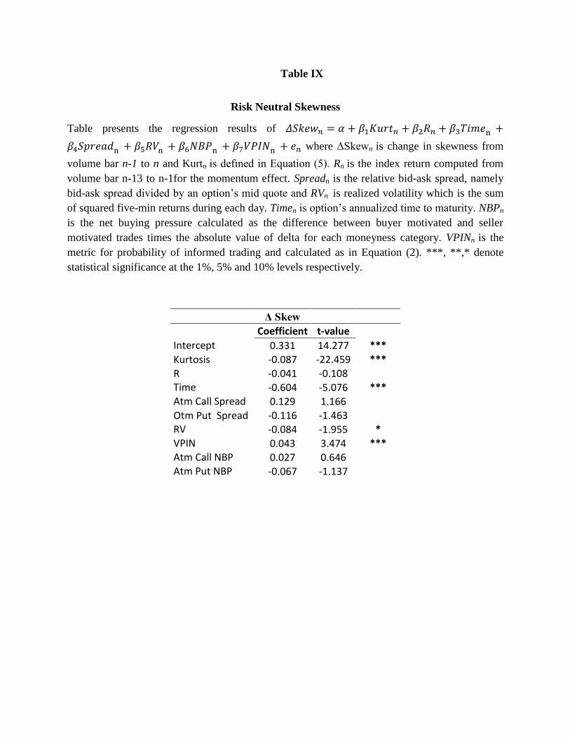
Table IX

Risk Neutral Skewness

Table presents the regression results of

where ΔSkewn is change in skewness from

volume bar n-1 to n and Kurtn is defıned in Equation (5). Rn is the index return computed from

volume bar n-13 to n-1for the momentum effect. Spreadn is the relative bid-ask spread, namely

bid-ask spread divided by an option’s mid quote and RVn is realized volatility which is the sum

of squared five-min returns during each day. Timen is option’s annualized time to maturity. NBPn

is the net buying pressure calculated as the difference between buyer motivated and seller

motivated trades times the absolute value of delta for each moneyness category. VPINn is the

metric for probability of informed trading and calculated as in Equation (2). ***, **,* denote

statistical significance at the 1%, 5% and 10% levels respectively.

Δ Skew

Coefficient t-value Intercept 0.331 14.277 ***

Kurtosis -0.087 -22.459 *** R -0.041 -0.108

Time -0.604 -5.076 *** Atm Call Spread 0.129 1.166

Otm Put Spread -0.116 -1.463 RV -0.084 -1.955 *

VPIN 0.043 3.474 *** Atm Call NBP 0.027 0.646

Atm Put NBP -0.067 -1.137