DETERMINATION OF SEA LEVEL TRENDS AND VERTICAL LAND MOTIONS FROM SATELLITE ALTIMETRY AND TIDE GAUGE OBSERVATIONS AT THE MEDITERRANEAN

COAST OF TURKEY

A THESIS SUBMITTED TO THE GRADUATE SCHOOL OF NATURAL AND APPLIED SCIENCES

OF MIDDLE EAST TECHNICAL UNIVERSITY

BY

SITAR KARABİL

IN PARTIAL FULFILLMENT OF THE REQUIREMENTS FOR

THE DEGREE OF MASTER OF SCIENCE IN

GEODETIC AND GEOGRAPHIC INFORMATION TECHNOLOGIES

DECEMBER 2011

Approval of the thesis:

DETERMINATION OF SEA LEVEL TRENDS AND VERTICAL LAND MOTIONS FROM SATELLITE ALTIMETRY AND TIDE GAUGE OBSERVATIONS AT THE MEDITERRANEAN COAST OF TURKEY

Submitted by SITAR KARABİL in partial fulfillment of the requirements for the degree of Master of Science in Geodetic and Geographic Information Technologies Department, Middle East Technical University by,

Prof. Dr. Canan Özgen Dean, Graduate School of Natural and Applied Sciences

Assoc. Prof. Dr. Ayşegül Aksoy Head of Dep., Geodetic and Geographic Info. Technologies

Prof. Dr. Mahmut Onur Karslıoğlu Supervisor, Civil Engineering Department, METU

Dr. Coşkun Demir Co-Supervisor, General Command of Mapping - Retired Examining Committee Members:

Assoc. Prof. Dr. Zuhal Akyürek Civil Engineering Department, METU

Prof. Dr. Mahmut Onur Karslıoğlu Civil Engineering Department, METU

Dr. Coşkun Demir General Command of Mapping - Retired

Assoc. Prof.Dr. Ali Kılıçoğlu General Command of Mapping - Retired

Assoc. Prof. Dr. Mehmet Lütfi Süzen Geological Engineering Department, METU

Date: 16/ 12/2011

iii

I here by declare that all information in this document has been obtained and presented in accordance with academic rules and ethical conduct. I also declare that, as required by these rules and conduct, I have fully cited and referenced all material and results that are not original to this work.

Name, Last Name: Sıtar Karabil

Signature:

iv

ABSTRACT

DETERMINATION OF SEA LEVEL TRENDS AND VERTICAL LAND MOTIONS FROM SATELLITE ALTIMETRY AND TIDE GAUGE OBSERVATIONS AT THE

MEDITERRANEAN COAST OF TURKEY

Karabil, Sıtar

M.Sc., Department of Geodetic and Geographic Info. Technologies

Supervisor: Prof. Dr. Mahmut Onur Karslıoğlu

Co-Supervisor: Dr. Coşkun Demir

December 2011,103 Pages A radar altimetry satellite measures the height of sea surface globally.

However, tide gauges, measuring Sea Level Height (SLH), are set up on

the Earth surface. Hence, SLHs are involved in vertical motion of the

Earth crust. In this study, vertical motions of Earth crust have been

separated from sea level variations.

After clustering of SSH observations with K-means approach, two outlier

detection methods Pope and Interquartile (IQR) Tests are implemented

in data. Afterwards, each altimetry measurement is relocated to the

center point of own cluster by means of geoid height derived from Earth

Gravitational Model 2008 (EGM08). Before application of Principal

Component Analysis (PCA) to see behavior of SSH inbetween clusters,

Lomb Scargle algorithm is run to realize power spectrum of every

clustered observations distinctly.

Besides, tide gauge measurements are used for extracting 68

constituents with T_Tide program from hourly tide gauge observations.

Then, predicted signal is produced by means of classical tidal harmonic

analysis. To get monthly and daily mean values of hourly data, MSDOS

v

Processing and Quality Controlling Software (SLPR2) has been run and

the results are compared with Permanent Service for Mean Sea Level

(PSMSL) monthly mean sea level values. Afterwards, the trends from

altimetry, tide gauge and GPS are investigated to reveal vertical land

motion.

This study shows that sea level is rising every year more or less 7 mm at

the Mediterranean coast of Turkey. Although İskenderun tide gauge

subsides 50 mm every year, the other stations do not show huge amount

of vertical motion.

Keywords: Satellite Altimetry, Tide Gauge, Sea Level Trends, Vertical

Motion.

vi

ÖZ

UYDU ALTİMETRESİ VE MAREOGRAF İSTASYONLARI GÖZLEMLERİ İLE

TÜRKİYE’NİN AKDENİZ KIYISINDA DENİZ SEVİYESİ TRENDLERİNİN VE

DÜŞEY YER KABUĞU HAREKETLERİNİN BELİRLENMESİ

Karabil, Sıtar

Yüksek Lisans, Jeodezi ve Coğrafi Bilgi Teknolojileri

Tez Yöneticisi: Prof. Dr. Mahmut Onur Karslıoğlu

Ortak Tez Yöneticisi: Dr. Coşkun Demir

Aralık 2011,103 Sayfa

Bir radar altimetre uydusu Deniz Yüzeyi Yüksekliği’ni (DYY) global olarak

ölçer. Ancak, Deniz Seviyesi Yüksekliği’ni (DSY) ölçen mareograf

istasyonları yeryüzeyi üzerine kurulmuştur. Bu nedenle DSY verileri yer

kabuğunun düşey hareketini de içerir.Bu çalışmada, yer kabuğunun

düşey hareketleri deniz seviyesi değişimlerinden ayrıştırılmıştır.

DYY gözlemlerinin K-means yaklaşımıyla kümelendirilmesinden sonra

uyuşumsuz ölçülerin tespiti için veri Pope ve interkartil testleri

yapılmıştır. Daha sonra, her bir altimetre ölçüsü Yer Gravite Modeli 2008

(YGM08)’den elde edilen geoid yükseklikleri aracılığıyla kendi kümesinin

merkez noktasına taşınmıştır. DYY’nin kümeler arasındaki davranışını

ortaya koymak için Temel Bileşenler Analizi (TBA) uygulanmadan önce

kümelenmiş her gözlemin güç spekturumu Lomb Algoritması yürütümü

ile açık bir şekilde ortaya konmuştur.

vii

Bununla birlikte, saatlik mareograf deniz seviyesi gözlemleri kullanılarak

68 adet gelgit bileşeni T_Tide program ile elde edilmiştir. Daha sonra

klasik gelgitsel harmonik analiz kullanılarak kestirim sinyali üretilmiştir.

Saatlik deniz seviyesi gözlemlerinden günlük ve aylık deniz seviyesi

değerleri elde etmek için SLPR2 yazılımı kullanılarak sonuçlar PSMSL’den

elde edilen aylık ortalama değerlerle kıyaslanmıştır. Son olarak, düşey

yer kabuğu hareketlerini ortaya çıkarmak için altimetri, mareograf ve

GPS trendleri irdelenmiştir.

Bu çalışma Türkiye’nin Akdeniz kıyısında her yıl 7 mm civarında bir deniz

seviyesi artışı olduğunu göstermektedir. Her ne kadar İskenderun

mareograf istasyonunda yıllık 50 mm’lik bir çöktüğü tespit edilse de

diğer istasyonlarda büyük bir düşey hareket görülmemektedir.

Anahtar Kelimeler: Uydu Altimetresi, Mareograf, Deniz Seviyesi

Trendleri, Düşey Hareket.

viii

To My Mother and My Deary Friend Kamuran Çakır

ix

ACKNOWLEDGEMENTS

I am greatly indebted to Mahmut Onur Karslıoğlu for his supervision,

friendly and wisdom advices and scientific suggestions which give

direction to my studies.

I am also indebted to Coşkun Demir for his supports and

encouragements, which helped me whenever I felt hopeless. I have

enormously benefited from his scientific teachings and minded arguments

on the data processing.

Special thanks go to Ali Kılıçoğlu for his support and encouragement and

for sharing his profound knowledge in related subjects of this thesis.

I also thank to examining committee members Zuhal Akyürek, Mehmet

Lütfi Süzen for their valuable comments and contributions.

I would like to take this opportunity to thank Civil Engineering

Department, Geomatics Division participants for their understanding and

contributions during my thesis studies, especially my roommate Armin

Aghakarimi.

Last but not least, I would like to express my deepest thanks to Eren

Erdoğan and Özkan Yılmaz who have not left me lonely in any challenging

condition since 2005.

x

TABLE OF CONTENTS

ABSTRACT ..................................................................................... iv

ÖZ ................................................................................................ vi

ACKNOWLEDGEMENTS .................................................................... ix

TABLE OF CONTENTS ....................................................................... x

LIST OF TABLES ............................................................................. xii

LIST OF FIGURES .......................................................................... xiv

CHAPTERS ...................................................................................... 1

1.INTRODUCTION ......................................................................... 1

1.1 Background ...................................................................... 1

1.2 Motivation......................................................................... 5

1.3 Study Area ....................................................................... 7

1.4 Thesis Outline ................................................................... 9

2.SATELLITE ALTIMETRY .............................................................. 10

2.1 Introduction .................................................................... 10

2.2 Missions ......................................................................... 13

2.3 Products of Altimetry Missions ........................................... 15

2.4 Used Missions and Data .................................................... 15

3.QUALITY CONTROL, ANALYSIS AND INTERPOLATION OF ALTIMETRY DATA ........................................................................................ 18

3.1 Creating BIN and Clustering of Observations ....................... 18

3.2 Statistical Tests on Data ................................................... 20

3.3 Selecting Outlier Detection Method .................................... 23

3.4 Interpolation of SSH Data ................................................. 24

3.5 Time Domain Interpolation of SSH Time Series .................... 26

3.6 Spectral Analysis of SSH Data ........................................... 28

3.7 Principle Component Analysis (PCA) on SSH ........................ 30

4.TIDE GAUGE DATA and PROCEDURE .......................................... 40

4.1 Introduction .................................................................... 40

xi

4.2 Products of A Tide Gauge .................................................. 41

4.3 Tide Gauge Data .............................................................. 43

4.4 Harmonic Analysis on Tide Gauge Data ............................... 45

4.5 Filtering of Hourly Data .................................................... 50

5. DETERMINING VERTICAL TRENDS ............................................. 56

5.1 Trends From Tide Gauges and Altimetry Satellites ............... 56

5.2 GPS Solution ................................................................... 59

5.3 Determination of Sea Level Trends and Vertical Land Motions 61

6. RESULTS ................................................................................ 65

6.1 Discussion on Trend Progress ............................................ 65

6.2 Evaluation of the Results .................................................. 67

7. CONCLUSION AND RECOMMENDATIONS .................................... 70

REFERENCES ................................................................................ 73

APPENDICES ................................................................................. 78

A: Flow Chart of The Study .......................................................... 78

B: Clusters of Altimetry Observations ............................................ 79

C: Cluster Similarities .................................................................. 81

D: Cluster Trends ....................................................................... 84

E: Standard Deviations of Clusters Before and After Centered .......... 88

F: Geodetic Coordinates (WGS84) of Cluster Centers ...................... 92

G: Significant Periods of Each Cluster ............................................ 96

H: Leading Three Spatial Models of Variability of Chosen Clusters ....100

xii

LIST OF TABLES

TABLES

Table 1 Altimetry Missions .............................................................. 14 Table 2 Used Data from AVISO ........................................................ 16 Table 3 Number of Clusters with Appropriate PEB Value ..................... 24 Table 4 Std. of SSH Observations Before and After Centered ............... 26 Table 5 Comparison of Std. between Cubic Spline and Lomb Scargle .... 30 Table 6 PCA results for Pass 159 ..................................................... 33 Table 7 Most Similar and Coast Cluster Data Groups .......................... 37 Table 8 SSH Trends and Test Values of Pass 159 ............................... 39 Table 9 Application Areas of Tide Gauge Data .................................... 42 Table 10 Used Tide Gauge Data ....................................................... 43 Table 11 Hourly Data Flags for Error Classification ............................. 45 Table 12 Primary Tidal Constituents ................................................. 47 Table 13 Significant Tidal Constituents of Erdemli Station (2003-2010) 49 Table 14 Standard Deviation of Difference in Original & Predicted Data 50 Table 15 Calculated & PSMSL MSL for Erdemli, 2009 .......................... 52 Table 16 MSL Values for Antalya 2006 .............................................. 53 Table 17 Used frequencies for SLH Trends ........................................ 57 Table 18 SLH Trends from Tide Gauge Observations .......................... 58 Table 19 SSH Trends from Altimetry Observations ............................. 58 Table 20 TheYears of GPS Campaigns .............................................. 60 Table 21 GPS Positions and Trends .................................................. 60 Table 22 GPS Velocities .................................................................. 61 Table 23 Comparison of Vertical Trends ............................................ 63 Table 24 Pass 68 Cluster Similarities ................................................ 81 Table 25 Pass 159 Cluster Similarities .............................................. 82 Table 26 Pass 170 Cluster Similarities .............................................. 82 Table 27 Pass 246 Cluster Similarities .............................................. 83 Table 28 Cluster Trends of Pass 68 .................................................. 84 Table 29 Cluster Trends of Pass 159 ................................................ 85 Table 30 Cluster Trends of Pass 170 ................................................ 86 Table 31 Cluster Trends of Pass 246 ................................................ 87 Table 32 Before and After Centered Standard Dev. of Pass 68 ............. 88 Table 33 Before and After Centered Standard Dev. of Pass 159 ........... 89 Table 34 Before and After Centered Standard Dev. of Pass 170 ........... 90

xiii

Table 35 Before and After Centered Standard Dev. of Pass 246 ........... 91 Table 36 Geodetic Coor. of Cluster Cent. for Pass 68 .......................... 92 Table 37 Geodetic Coor. of Cluster Cent. for Pass 159 ........................ 93 Table 38 Geodetic Coor. of Cluster Cent. for Pass 170 ........................ 94 Table 39 Geodetic Coor. of Cluster Cent. for Pass 246 ........................ 95 Table 40 Significant Periods of Pass 68 ............................................. 96 Table 41 Significant Periods of Pass 159 ........................................... 97 Table 42 Significant Periods of Pass 170 ........................................... 98 Table 43 Significant Periods of Pass 246 ........................................... 99

xiv

LIST OF FIGURES

FIGURES

Figure 1 Flowchart of the Study ......................................................... 7 Figure 2 Tide Gauge Stations ............................................................ 7 Figure 3 Chosen Theoretical Tracks .................................................... 8 Figure 4 Principle of Radar Altimetry ................................................ 12 Figure 5 Sample Satellite Tracks Produced by BRAT ........................... 17 Figure 6 Pass 159 T/P, J-1 Clustering Sample .................................... 20 Figure 7 Each Measured SSH is brought to its Center ......................... 25 Figure 8 A Sample of Cubic Spline Interpolation, J1-T/P Pass159 ......... 27 Figure 9 A Sample Lomb Power Spectrum for J1-T/P, Pass 159 ........... 29 Figure 10 Leading Three Spatial Models of Variability (eigenvectors)(Clusters 4-8) ........................................................... 34 Figure 11 Leading Three Spatial Models of Variability (eigenvectors)(All Clusters) ...................................................................................... 35 Figure 12 Leading Three Principal Components (temporal modes of variability) .................................................................................... 36 Figure 13 All Clusters of Pass 159 .................................................... 38 Figure 14 A Tide Gauge Measurement System ................................... 41 Figure 15 A Sample of Hourly TG Data Format .................................. 44 Figure 16 Clusters of Pass 68 .......................................................... 79 Figure 17 Clusters of Pass 159 ........................................................ 79 Figure 18 Clusters of Pass 170 ........................................................ 80 Figure 19 Clusters of Pass 246 ........................................................ 80 Figure 20 Leading Spatial Models for Pass 68 ...................................100 Figure 21 Leading Spatial Models for Pass 159 ................................101 Figure 22 Leading Spatial Models for Pass 170 ................................101 Figure 23 Leading Spatial Models for Pass 246 ................................101

1

CHAPTERS CHAPTER 1

1.INTRODUCTION

1.1 Background

Altimetry satellites were started to be launched in the early 1970s. First

mission called Skylab was launched in May 1973. Then, the other

altimetry satellites are succeeded such as GEOSAT, ERS-

1.TOPEX/POSEIDON, GFO, ERS-2, Jason-1. ENVISAT, Jason-2, and also

six more satellites will be on duty in the near future (Benveniste and

Picot 2011).

A radar altimeter obtains data about the shape of the Earth globally.

These measurements give rise to perform different kind of altimetry

applications such as geodesy, geophysics, ocean, ice, climate,

atmosphere, wind, waves, hydrology and coastal studies. It is generally

known that geodesy is the science of the Earth's shape and size. If the

matter of geodesy is to determine external gravity field of the Earth, it

can be said that the precise knowledge of the physical size and shape of

the sea surface is an important factor of the problem. If the problem of

physical oceanography is to monitor the temporal variations of the sea

surface, a global high-accuracy high-resolution mean sea surface (MSS)

model can play key role in absolute oceanic datum for this purpose.

Satellite altimetry measures the real shape of the oceans directly. The

precision of altimeter SSHs has progressed from SKYLAB to the

TOPEX/POSEIDON. The accuracy and resolution of MSS models have

been improved across all spatial and temporal scale by means of better

2

precision and spatial coverage of the altimeter measurements (Fu and

Cazenave 2001).

A tide gauge measures sea level height (SLH) at the coastline fixed to the

Earth surface. As a result of continuously observation of sea level, tide

gauge measurements can be used in the area of geodesy, geophysics,

geology, oceanography, climatology, meteorology, water resource

management, hydrology, sailing, coastal risk management, human and

environmental security in order to run different applications related with

water ascent and descent. There are more than two thousand tide

gauges over the world (PSMSL 2011).

Turkey, with responsibility of General Command of Mapping (GCM) has

eleven tide gauges. Basically tide gauge network is to define SLH at the

coastal line. The first tide gauge station was set up at Antalya Harbor in

1936. After that date there were some studies to define zero level for

national vertical control network in Turkey. At present Turkish National

Sea Level Monitoring System (TUSELS) has Ankara data center and tide

gauge stations namely Antalya-II, Erdemli, Bozyazı, Taşucu, İskenderun,

Girne, Bodrum-II, Menteş, Erdek, Amasra, Trabzon-II, İğneada, Sinop,

Gökçeada, Şile, Marmara Ereğlisi, Aksaz, Gazimağusa and Şile (Yıldız, et

al. 2003), (H. Yıldız 2001).

Since tide gauge measures the relative motion between sea surface and

the ground where station is located at, the problem of relative motion

must be eliminated to use SLH meaningfully (H. Yıldız 2001), (Carrera

and Vanicek 1985). To separate sea level change resulting from sea level

variations from vertical land motion, it can be said that analysis of sea

level variations does not give sufficient results before correcting them

with external source like satellite altimetry data. Sea level trends are also

useful to define vertical crustal motion, if ancillary information source is

considered (Carrera and Vanicek 1985), (IOC 2000).

3

Long-term sea-level change has been estimated from tide gauge

measurements more than the last century. However, two fundamental

problems have been come out when using tide gauge measurements for

this purpose. First, tide gauges only measure sea level change relative to

a crustal reference point, which may move vertically at rates comparable

to the true sea-level signals (Douglas 1995). Second, tide gauges have

limited spatial distribution and suboptimal coastal locations, and thus

they provide poor spatial sampling of the SSH (T. Barnett 1984), (Groger

and Plag 1993).

An independent global measurement technique is needed to investigate

the important issues associated with SSH change. In principle, satellite

altimeters should provide improved measurements of global sea-level

change over shorter averaging periods because of their truly global

coverage and direct tie to the Earth’s center of mass (Fu and Cazenave

2001).

Satellite altimeters provide a measure of absolute sea level relative to a

precise reference frame realized through the satellite tracking stations

whose origin coincides with the Earth’s center of mass (Nerem, et al.

1998).

(Marc, Dietz and Groten 2004) have computed estimates of the rate of

vertical land motion in the Mediterranean Sea from differences of sea

heights measured by the TOPEX/Poseidon radar altimeter and by a set of

tide gauge stations. Afterwards, they have predicted absolute vertical

land motion in the Mediterranean Sea relative to the geocenter by

computing the linear term of the differences of altimetry and tide gauges

SLH time series.

Additionally, (Kuo and Shum 2004) have shown some combining results

regarding the subject. They presented a new method of combining

satellite altimetry and tide gauge data to obtain improved estimates of

absolute vertical crustal motion at tide gauges within a semi-enclosed

4

sea. As an illustration, they have combined T/P altimetry data and 25 tide

gauge records around the Baltic Sea Region of Fennoscandia.

(Garcia, et al. 2007) compared tide gauge data with SSH anomaly

obtained from T/P and ERS-1/2 for a period of 1993-2001. They have

estimated vertical ground motion, for each tide gauge, from the slope of

the SSH time series of the difference between records and the altimetry

measurement at a point closest to the tide gauge.

(Mitchum 1994) studied on comparison of tide gauge and altimetry

measurements with some statistical assessments. Then, Mitchum has

reached some results regarding tidal constituents and precision of

measurements. On the other hand, (C. Kuo, et al. 2008) presented a new

robust technique to estimate absolute vertical motion using both satellite

altimetry and tide gauge records in Fennoscandia, Alaskan coast, and the

Great Lakes.

(Nerem and Mitchum 2002) have computed estimates of the rate of

vertical crustal motion from differences of sea level measurements made

by the TOPEX/POSEIDON radar altimeter and a globally distributed

network of 114 tide gauges. In that study, a rigorous error analysis was

performed which suggests the accuracy of the estimated vertical rates is

approximately 1-2 mm/year for roughly half of the tide gauges, which is

sufficiently accurate to detect a variety of geophysical phenomena.

Moreover, (Braitenberg, et al. 2010) examined tide gauge and satellite

altimetry observations of sea level with the aim of obtaining crustal

vertical movement rates. The correction of the tide gauge data sea level

rates for the SSH contribution requires collocation of the satellite pass

and the tide gauge station. They showed that the satellite altimetry

observations enable correction of differential tide gauge rates for the

effects of sea surface rate inhomogenities. Coastal sea level trends can

be defined with the comparison of altimetry and tide gauge observations.

5

(Mangiarotti 2007)has made a joint analysis with using T/P satellite

altimetry and tide gauge data to estimate sea level trends along the

Mediterranean Sea coast from 1993 January to 2002 February. To detect

long-term sea level change, (L. F. Marc 2002) has gathered data of T/P,

ERS-1/2 missions and from tide gauge data. In that study, long-term sea

level change during 1992-2000 is investigated in the Mediterranean Sea.

1.2 Motivation

In this study, T/P, Jason-1 satellite missions are used to extract altimetry

measurements from Basic Radar Altimetry Toolbox (BRAT) which is

developed by European Space Agency (ESA) and Centre National

d’Etudes Spatiales (CNES). The data is obtained from Archiving,

Validation and Interpretation of Satellite Oceanographic Data (AVISO).

After getting the proper data according to its space and time, processes

have been implemented in MATLAB R2010b. These processes include

• clustering of data,

• outlier detection tests and comparisons of methods,

• significant test of parameters,

• interpolation of SSHs with respect to their spatial distribution with

the aid of geoid height,

• spectral and time domain analysis of altimetry data,

• Principle Component Analysis (PCA) of altimetry data,

• Determination of SSH trends.

To get the geoid height, Earth Gravitational Model 2008 (EGM08) has

been taken as the model.

Tide gauge data have been obtained from GCM. Within this study four

tide gauge stations have been used to investigate sea level trends and

vertical land motions of tide gauge stations. Tide gauge hourly data is

analyzed with classical tidal harmonic analysis model, then significant

6

tidal constituents have been defined to get predicted signal (Pawlowicz,

Beardsley and Lentz 2002). Predicted signal is needed to full data gaps in

hourly data. Hourly data, to be able to compare with altimetry

observations, has been filtered to make it for daily and monthly data with

the help of SLPR2 software ((SLC) 2011).

Afterwards, SSH trends are extracted from the information of similarity

percentage derived from PCA method on altimetry observations. Since

sea surface is assumed as homogenous in small area, the most common

group of cluster has been considered to compute SSH trends. Also,

almost all clusters, excluding last three clusters, have been taken into

account to calculate SSH trends of each Pass. Then, difference rates of

SSHs-SLHs are defined to be able to figure out sea level trends and

vertical crustal movements of tide gauge stations. To see the SSH trends

of each Pass, for the SSH trend derived from chosen clusters, arithmetic

mean of chosen clusters is accepted as SSH trend. On the other hand, at

the second approach only excepting last three clusters, SSH trend has

been calculated from linear regression of first principal component.

The scope of this study is to find mainly vertical crustal motion of the

Bodrum, Antalya, Erdemli and İskenderun tide gauges and partly SSH

and SLH trends on the North Eastern Mediterranean Sea. The flowchart of

this study can be seen in Figure 1.

7

1.3 Study Area

Study area is located roughly between 35°N-37°N latitude, and 27°E-

36°E longitude. This means thatstudy area is North-Eastern

Mediterranean Sea, especially the Mediterranean coast of Turkey.

In this study, the tracks of T/P and Jason-1 like 68, 159, 170 and 246

have been chosen for Erdemli, İskenderun, Bodrum and Antalya

respectively. Tide gauge stations can be seen in Figure 2.

Figure 2 Tide Gauge Stations

Figure 1 Flowchart of the Study

8

Theoretical tracks of altimetry missions are shown in Figure 3.

Figure 3 Chosen Theoretical Tracks

9

1.4 Thesis Outline

This thesis consists of seven chapters. Background and objectives of

study are explained in Chapter1.

Chapter 2 is dedicated to give brief information about satellite altimetry

and its missions, used software, products and content of data which are

obtained by a mission.

Quality control, interpolation and analysis of altimetry data are handled in

Chapter 3. As subtopic, BIN method and clustering are mentioned, and

statistical tests have been applied to data with detection of outlier and

significance of trend parameters. Each altimetry measurement is brought

to its center with respect to geoid undulation. Afterwards, time domain

and frequency domain analysis have been implemented in SSH data for

interpolation detailed in this chapter. Lastly, evaluation of PCA is the

result of this chapter.

Tide gauge data and related products are presented in Chapter 4. Also, to

define tidal constituents and fulfill data gaps, harmonic analysis has been

applied to hourly data.

Determining Vertical Trends, Chapter 5, which covers determination of

vertical trends and extracting crustal motions on the tide gauges are

contained. SSH trends and SLH trends have been defined and compared

to see the vertical trends and vertical crustal motion for each tide gauge

points. Also, brief information about GPS technique is given here.

The results are discussed and evaluated in Chapter 6. Within this purpose

results are investigated in different views.

A concluding remark and future works are indicated in Chapter 7 with a

summary.

10

CHAPTER 2

2.SATELLITE ALTIMETRY

2.1 Introduction

Altimetry is a kind of technique for measuring SSH directly according to a

reference frame. Satellite radar altimetry measures time of a signal

produced by a radar pulse round-trip from the satellite to surface of the

Earth and return to the receiver of the same satellite. Moreover, this

measurement yields amount of other information that can be used for a

wide range of applications.

The principle is that the altimeter emits a radar wave and analysis the

bounced off signal from the Earth surface. SSH is the difference between

position of satellite with respect to an arbitrary reference surface

(altitude) and satellite-to-surface distance (range) calculated by

measured time. The time is period of signal between satellite and the

Earth round trip. Besides SSH, by looking at the return signal's amplitude

and waveform, we can also measure wave height and wind speed over

the oceans, backscatter coefficient and surface roughness.

If the altimeter emits in two frequencies, the comparison between the

signals, with respect to the used frequencies, can also generate

interesting results like rain ratio on the oceans, over ice shelves,

detection of crevasses etc.

To obtain accurate measurements within a few centimeters from a range

of several hundred kilometers requires an extremely precise knowledge

11

of the satellite position. Thus several locating systems are usually

embedded onboard altimetry satellites. Any interference with the radar

signal also needs to be taken into account. Water vapor and electrons in

the atmosphere, sea state and a range of other parameters can affect the

signal travel time, thus distorting range measurements. We can correct

these interference effects on the altimeter signal by measuring them.

There are three main methods to bring correction on these effects like

embedding supporting instruments into satellite, using several different

frequencies on satellite, modeling the effects.

Altimetry requires an amount of information to be considered before

being able to use the data. Namely, data preprocessing is also a major

part of altimetry, producing data of different levels optimized for different

uses.

Radar altimeters on board the satellite transmit signals at high

frequencies (over 1.700 pulses per second) to Earth, and receive the

echo from the surface. This is analyzed to derive a precise measurement

of the time taken to make the round trip between the satellite and the

surface. This time measurement, scaled to the speed of light, the speed

at which electromagnetic waves travel, yields a range R measurement.

The ultimate aim is to measure surface height relative to a terrestrial

reference frame. The principal of satellite altimetry can be seen in Figure

4 (Benveniste and Picot 2011).

12

The important parameters of orbit for satellite altimeter missions are

inclination, altitude, and period. The period is the time needed for the

satellite to pass over the same position on the Earth surface. Inclination

gives the highest latitude where the satellite can measure the Earth.

The altitude of a satellite is the distance of satellite with respect to a

predefined reference surface. It is up to amount of limitations like

inclination, atmospheric drag, gravity forces, field of the world to be

mapped. The satellite can be tracked in several approaches to measure

its altitude with the best possible accuracy, so determine its precise orbit,

accurate within 1 or 2 cm. So that SSH measurement can reach

toapproximately 4 cm accuracy for both T/P and Jason-1.To achieve the

Figure 4 Principle of Radar Altimetry (Benveniste and Picot 2011)

13

goal for SSH accuracy (2.5 cm root-mean-square -RMS), radial orbit

errors must be reduced to 1 cm (RMS) (CalVal, AVISO 2011).

The SSH is the distance of satellite at a measurement time from the

defined reference surface, so:

SSH = Satellite Altitude – (Altimeter Range + Corrections).

To deduce the dynamic topography, the easiest solution could be to

subtract the geoid height from SSH. But in practice, mean sea level is

subtracted, to determine the sea level anomalies of the ocean signal.

Several different frequencies are used for radar altimeters. The choice

depends upon regulations, mission objectives and constraints and

technical possibilities. Each frequency band has its advantages and

disadvantages. These bands are Ku band (13.6 GHz),C band (5.3 GHz),S

band (3.2 GHz),Ka band (35 GHz). (Benveniste and Picot 2011)

2.2 Missions

Missions classification can be made based on the expire and launch date

of them. With this point of view there are three main parts to mention:

past missions, current missions and future missions. While Geosat, ERS-

1, Topex/Poseidon, GFO are past missions, ERS-2, Jason-1, Envisat,

Jason-2, Cryosat are present missions. Scheduled future missions are

Saral, HY-2, Sentinel 3, Jason-3. The missions are detailed in following

table, Table 1 (Benveniste and Picot 2011).

14

Table 1 Altimetry Missions

By means of satellite altimetry missions, we are able to view the Earth

and its open and semi-closed seas from the vantage point in space. Thus,

measurements obtained from altimetry missions give an advantage to

observe sea surface of Earth globally and frequently.

Satellite Launch Mission Frequency Altitude Inclinati

on

SkyLab 1973 Acquiring new knowledge in Space to improve life on Earth

435 km 50°

GEOS 3 1975 Geodesy 845 km 115° Seasat 1978 Study Earth

and its Seas Ku Band 800 km 108°

Geosat 1985 Describing marine geoid

Ku Band 800 km 108°

ERS-1 1991 Observe Earth and its Environment

Ku Band 785 km 98.5°

T/P 1992 Measure SSH Ku-C Band 1336 km 66° GFO 1998 Measure

ocean topography

Ku Band 800 km 108°

ERS-2 1995 Observe Earth and its Environment

Ku Band 785 km 98.52°

Jason-1 2001 Measure SSH Ku-C Band 1336 km 66° Envisat 2002 Observe

Earth’s atmosphere and surface

Ku-S Band 800 km 98.5°

Jason-2 2008 Measure SSH Ku-C Band 1336 km 66° Cryosat 2010 Polar

observation Ku Band 720 km 92°

Saral 2012 Measure SSH Ka Band 800 km 92° HY-2 2011 Observe the

ocean dynamics

Ku-C Band 963 km 99.3°

Sentinel 3

2013 Provide operational oceanography data for GMES

Ku-C Band 814 km 98.5°

Jason-3 2013 Measure SSH Undefined dual frequency

1336 km 66°

(Benveniste and Picot 2011)

15

2.3 Products of Altimetry Missions

There is wide range of data and software to be used in altimetry

applications. Products as data can be derived from an altimetry mission.

These products generally are sea surface height, significant wave height,

sea surface height anomaly, sea level anomaly, bathymetry, sea surface

temperature, range, mean sea surface, wind speed and dynamic ocean

topography. Additionally, gravitational potential and regarding products,

like disturbing potential, gravity, gravity anomaly, gravity gradiant, can

be derived from sea surface height information in different platforms like

Geopot 2007.

In addition to data product, there is a broad range of software to be used

in altimetry applications. Basic Radar Altimetry Toolbox (BRAT),

PublicReadBinaries, SSHA software, OPR reading software, Modified

Chelton-Wentz model, EnviView, Envisat L2 RA2-MWR Products Read and

Write Software and Convert programs for waveforms POSEIDON products

can be emphasized as main altimetry software products (Benveniste and

Picot 2011).

2.4 Used Missions and Data

Considering study area and time span, two different altimetry missions

are chosen to obtain altimetry data. These missions are Jason-1and

Topex/Poseidon. Additionally, BRAT developed by CNES and ESA is taken

as altimetry software product within this study. Besides, AVISO corrected

SSH data obtained from (AVISO 2011) is explained below in Table 2. The

altimeter products were produced by CLS Space Oceanography Division

and distributed by AVISO, with support from CNES.

16

Table 2 Used Data from AVISO

Altimetry measurements need to be corrected for instrumental errors,

environmental perturbations like wet tropospheric, dry tropospheric and

ionospheric effects. Also, the ocean sea state influence, the tide influence

and atmospheric pressure must be considered to be corrected. With this

aim AVISO has brought the most renewed residuals into altimetry data.

Thus, the applied residuals are orbit, dry troposphere, wet troposphere,

Ionosphere, sea state bias, ocean and loading tides, solid Earth tide, pole

tide, combined atmospheric correction, major instrumental correction (H.

AVISO 2011).

In this study, these data are processed in BRAT software. As mentioned

above, BRAT software is advanced with the responsibility of ESA/CNES.

BRAT is a tool to run the processing of radar altimetry data. Besides,

BRAT is able to treat so many radar altimetry data formats, providing

support for processing, editing, extracting statistics, visualizing and

exporting the outputs.

BRAT covers some modules operating at different levels of abstraction.

These modules can be Graphical User Interface (GUI) applications,

command-line tools, interfaces to applications like MATLAB or application

program interfaces (APIs) to programming languages such as C and

Fortran (ESA and CNES 2011). Sample outputs of BRAT are given in

Figure 4.

Satellite Data Time Interval Data Period Jason-1 February 2002 – January 2009 10 days T/P January 1999 – February 2002 10 days

17

Figure 5 Sample Satellite Tracks Produced by BRAT

18

CHAPTER 3

3.QUALITY CONTROL, ANALYSIS AND INTERPOLATION OF ALTIMETRY DATA

3.1 Creating BIN and Clustering of Observations

BIN data structure developed by (Bosch and Savcenko 2005) is the

reorganization of satellite altimeter data to perform time series analysis.

BINs are clusters along ground track of the altimeter satellite. Their

positions are defined according to equator crossing of the ground track of

altimeter satellite. To be able to have at least one observation, each BIN

is separated by 1 Hz which means 7 km distance.

Numbering of BINs is given by bin Id number. This Id number is defined

with respect to the equator crossing. binid = 0 means that the center of

that BIN is crossing of the equator with the ground track. For ascending

satellite pass BIN numbers are negative at the south of the equator, and

BINs are positive at the north of the equator. Besides, for the descending

pass of any satellite mission vice versa.

For example, BINs are divided into 3101 parts from -1500 to +1500. For

ascending pass of T/P first number will be -1500 and last number will be

-1 before the equator, and it continues with the same approach for north

side of the equator (Bosch and Savcenko 2005).

In this study, BIN data structure is handled as a sample method to

explain clustering sense of SSH data. To cluster the data K-means

19

approach has been applied. The K-means algorithm, very popular to

cluster the data, is developed by (MacQueen 1967) in 1967. K-means

searches for a proper segment of the data by minimizing the sum-of-

squared-error criterion with an iterative procedure (Xu ve Wunsch II

2009). The important part of this clustering method is to define distance

between data. K-means algorithm can compute similarity of 2D and 3D

data geometrically. Definition of cluster number is the weak point of K-

means algorithm because of depending on user’s choice. However,

ISODATA approach is introduced by (Ball and Hall 1967) deals with

dynamic prediction of cluster number. The steps of K-means clustering

method can be summarized as below.

i. Cluster centers are defined according to cluster numbers,

ii. The distance of each single point from each center is computed.

Then, all the data points are put into the clusters according to the

closest distance,

iii. Each center point of clusters is calculated again by means of

averaging of positions of all data points in cluster. Old center point

is relocated with the new one,

iv. Iterative computation in (ii) and (iii) arerepeated again till new

center point remains the same with previous one.

20

Each mission is clustered within this concept by means of generating the

required codes in MATLAB R2010b platform (Govaert 2009). A sample

clustered data can be shown in Figure 6, in which different color means

different clusters.

3.2 Statistical Tests on Data

To model and test data linear least square adjustment (LLSA) method

has been used as solution method. LLSA fitting method has huge amount

of place to adjust and model SSH data in different studies. LLSA is a kind

of method to estimate unknown parameters given by minimizing the sum

of the squares of residuals of the observations from estimated

parameters’ expected values. LLSA has major advantages to use

distributed data in spatial and in time. These advantages can be listed as

following (Koch 1999), (Pugh 1987).

• It does not depend on length of data

• Fitting procedure can be applied to data for any time span

• Data gaps do not limit the analysis

• No assumption is needed to perform fitting procedure

Figure 6 Pass 159 T/P, J-1 Clustering Sample

21

Least square estimation is used for the estimation of unknown

parameters on the basis of Gauss Markof Model which is given by

equation 3.1.

���� � � � ����� with ��� � 0 (3.1)

Hereby, n is number of observations, u is number of parameters, e

israndom measurement error which makes the equation consistent, y

represents observations, x is jacobian matrix. Note that measurements

are accepted as equally weighted and uncorrelated so that P = I. The

estimated parameters are obtained from equation 3.2.

� � ���� ����� (3.2)

The estimated residual is given in equation 3.3.

�� � �� � � (3.3)

Then, variance factor

���� � �������� (3.4)

Variance covariance matrix of the observations

��� � ��� � ����� (3.5)

For the assessment of the result variance covariance matrix of

parameters is also needed

D(�) =�������� �� (3.6)

Note that all these procedures have been made in every linear regression

steps for both SSH data and SLH data.

To understand the statistical distribution of data set and statistical

significance of model parameters, outlier detection and significance tests

have been implemented in each clustered data. An outlier can be defined

22

as a value that is numerically distant from the other data (Barnett ve

Lewis 1994), (Koch 1999). Standardized residual is

�� ,"=|�$|%�&√(�$�$ (3.7)

Here,σ�� is given as apposterori variance, *++ is weight coefficient matrix

of residuals, e-.,/ is standardized residual. For the implementation of Pope

Outlier test, tau distribution value is taken into account as table value.

Outlier is detected with the following expression

��012," 3 45,��6&/� (3.8)

To define the variation of observations with respect to time, second trend

function of least square adjustment model is being used (Wolberg 2006).

The statistical significance of trend parameters is tested based on Test t.

8 � �9�� (3.9)

Herein, � represents vector of parameters, 9�� is standard deviation of

parameters. T test accepts the parameters of trend function as

significance values, if computed t value is bigger than table t value.

With the scope of this study, two outlier detection methods have been

applied to the altimetry data. As mentioned above first one is Pope

Outlier test, and the second one is Interquartile (IQR) outlier detection

method.

IQR is based on median value of data. In IQR method, firstly the main

median (Q2) of the all data must be computed. Then, the low median

(Q1) and high median (Q3) are calculated. Q1 and Q3 are deduced from

the data which are less and greater thanmain median value, respectively.

Afterwards, the range (R) between the difference of Q1 and Q3 is

computed (Upton ve Cook 1996). A measurement (M.) is accepted as

outlier, if

23

M. 3 Q< � =<�> R or M. B Q� � =<�> R (3.10)

The results from IQR and Pope Test are checked out according to the

statistical criterion called as percentage error band (PEB) which is

explained in the next section.

3.3 Selecting Outlier Detection Method

Outliers detected by means of Pope Test and Interquartile are compared

cluster by cluster for selecting the best method with the value of PEB.

The PEB value is simple and useful method to be able to choose the

proper outlier detection method. For each cluster the PEB value is

calculated as follows (eHow 2011), (Tiwari, et al. 2007):

��C � DE�DFDE 100 (3.11)

In here, D is observation detected as outlier within its own cluster, D- is mean value of data in the cluster. The PEB values of detected outliers

show difference in Pope Test and IQR. It is appropriate to have

observations with the lower PEB value (Tiwari, et al. 2007), (Allison

1999).

Through PEB value approach, all data are examined by appropriate

outlier detection method. Note that the lowest PEB value is 1.57, the

greatest value is 9.34. It is resulted from PEB value approach that Pope

Test is dominantly better than IQR for the case. Totally, in only one

cluster Iqr method gave good result against with Pope. The number of

appropriate results can be seen in Table3.

24

Table 3 Number of Clusters with Appropriate PEB Value

3.4 Interpolation of SSH Data

After being progressed with respect to some statistical criterion like

outlier detection and significance test of the model, each data is brought

to the center of its cluster by means of geoid height extracted from Earth

Gravitational Model 2008 (EGM08) (Pavlis, et al. 2008).

hsynth_WGS84.f program has been used to calculate geoid undulations

from spherical harmonic synthesis of the EGM2008 Tide Free Spherical

Harmonic Coefficients and its correction model (Zeta-to-

N_to2160_egm2008). As input, user must give the latitude and longitude

of points where geoid undulations needed to be computed. Thus the

output includes latitude, longitude and geoid height of the points.

To process the interpolation procedure, geoid height is computed in every

point of data and at the position of each cluster center. Thereafter, geoid

height is used as slope surface with the linear calculation basis in the

form of following solution

HHIJKL � HHI � �MJ � M (3.12)

Here, HHI is the measured SSH of each point, M is the geoid height of

each measured point position, MJ is symbol to show the geoid heights of

each cluster center. The maximum value ofdistancebetween measured

Pass Number

Number of Pope

Dominated Clusters

Number of Iqr

Dominated Clusters

Number of Clusters

with Equal PEB Value

Number of Clusters with No Outlier

Detected 68 24 - - 7

159 8 - - 2 170 18 1 1 15 246 14 - 3 11

25

point position and the position of its cluster’s center was approximately 4

km. To illustrate, a sample figure is given in Figure 7.

After bringing the observations to their centers standard deviations of

clusters have been changed. This change is given in Table 4 for Pass 159.

Note that there is an enormous change of standard deviation in each

clustered data set. To illustrate, for Pass 246, before centered mean of

standard deviation is 0.1438 m., on the other hand, after centered

standard deviation becomes0.0909m. It makes sense that using geoid

height as slope surface is an applicable method on SSH relocation. All

standard deviations of relocated SSHs are given in Appendices part of

this study.

Figure 7 Each Measured SSH is brought to its Center

26

Table 4 Std. of SSH Observations Before and After Centered

Cluster Number Std. of SSHs Before Centered (cm)

Std. of SSHs After Centered (cm)

1 11.16 7.88 2 11.07 8.12 3 10.84 8.33 4 11.42 8.17 5 11.71 8.10 6 12.42 8.62 7 12.19 8.65 8 12.50 8.91 9 11.92 8.52

10 12.51 9.17

Afterwards, to be able to analyze data spectrally whole data must be

fulfilled with a proper method. In this study, PCA has been used to

analyze clusters and their similarities, thus, each cluster has been fulfilled

before PCA method is applied. With this aim, SSH values handled as a

time series signal to analyze.

After analyzing SSH as a time series signal, data gaps are fulfilled by two

kind of methods. This process has been performed based on time domain

and frequency domain approach. For time domain approach cubic spline

interpolation method has been run, on the other hand, for frequency

domain one Lomb-Scargle algorithm has been used in this study. Due to

becoming appropriate structure for unevenly spaced data, for time

domain; cubic spline, and for frequency domain; Lomb-Scargle methods

have been selected to implement in SSH time series.

3.5 Time Domain Interpolation of SSH Time Series

Since having gapped data in each cluster, SSH time series are analyzed

in time domain and spectral domain. As time domain solution, cubic

spline method has been chosen to interpolate SSH time series in each

cluster. Cubic Spline interpolation works well in condition of existing

gapped data (De Boor 2001).

27

As it is well known, a simple curve fit is based on one equation for all n

points. However, a cubic spline allowing each segment to have a unique

equation. In cubic spline, the routine fits n equations for n intervals

subject to the boundary conditions of n+1 data points. The form for the

cubic polynomial curve fit for each segment is given in equation 3.13.

� � N$�� � �$ O � P$�� � �$ Q � R$�� � �$ � S$ (3.13)

The routine must ensure that T�U , TV�U WXY TVV�U are equal at the interior

points for adjacent segments. In this study, x values are considered as

times, i is for gapped data, and y values are SSH observations. The cubic

spline parameters a,b,c,and d are defined from known observations to

interpolate data gaps at given time for each cluster.

The cubic spline is an easy to implement curve fit routine. Because the

method includes connecting individual segments, so that the cubic spline

avoids oscillation problems in the curve fit. After all, the cubic spline

provides good curve fit for unevenly spaced data points (Lilley 2002),

(O'Neill 2002).

A sample spline interpolation result is shown in Figure 8.

Figure 8 A Sample of Cubic Spline Interpolation, J1-T/P Pass159

28

While blue lines are for gapped data points, dashed red lines represent

cubic spline interpolation predictions.

3.6 Spectral Analysis of SSH Data

Any periodical signal in the timedomain can be deduced from the sum of

sine and cosine signals of different frequency and amplitude. This sum is

called as Fourier series. Fourier series represent a wave that repeats

itself. If the wave is complicated, it is the sum of simple waves

(Rauscher, Janssen and Minihold 2001), (LEX 2006).

Fast Fourier Transform is the most popular technique to transform the

signal into the frequency domain. However, if data have some gaps,

some other techniques like Lomb Scargle or McClean may be used to

analyze the data in frequency domain. Due to existing of gaps in data,

Lomb scargle algorithm is handled in this study.

Lomb scargle is a method to predict a frequency power spectrum through

a least squares fit of sinusoids to original data. This method is similar to

Fourier analysis. But Fourier analysis gives power spectrum of signal with

more noises than Lomb Scargle in the case of gapped data records

(Ibanoglu 2000), (Birney, Gonzalez and Oesper 2006), (Press, et al.

2007).

The Lomb Scargle method is also known as least square spectral analysis.

Simply, a periodogram is a prediction of spectral density of a signal.Lomb

Scargle uses Lomb Scargle Periodogramand least-squares fitting of

chosen frequencies of sinusoids computed from such periodograms

(LombScargle tarih yok). The method evaluates data, and sines and

cosines, only at times t. that are actually measured with given freqencies ω. (2∏f.). Then, predicts amplitude coefficients A and B to find SSH where

actual measurement has not gathered.

The lomb scargle can be presented as equation 3.15.

]^ � _`abc d � CbEXc d (3.15)

29

In this study, ω. is input frequency coming from measurement times, hf. is actual SSH data, A and B are coefficients of amplitude of signal

deduced from SSH time series.

One step before using amplitudes which are found by lomb scargle

method, there is a significance test must have been made on amplitudes

for each SSH time series. According to significance level (α), significant

amplitude and its frequency have been defined with alpha = 0.05

significance level. Also, the significant periods derived from significant

frequencies are deviating from 1 to 8 years. For further information, all

significant periods can be found at Appendices. It can be said that there

are some local periodical effects on SSHs which may not be modeled by

global ocean tide model (GOT 4.7). A sample resulting figure showing

Lomb Scargle Power spectrum can be seen in Figure 9. It represents first

cluster of Pass 159.

Figure 9 A Sample Lomb Power Spectrum for J1-T/P, Pass 159

30

After having interpolated SSH time series for gapped data times, a

comparison has been made among the results between cubic spline

interpolation and Lomb Scargle interpolation. As a general result,

standard deviations of Lomb Scargle outputs were approxiametly 1.5 cm

lower than cubic spline outputs. To illustrate, the standard deviation of

spline interpolated data set for one cluster was ±8.39 cm, while the

standard deviation of Lomb Scargle interpolated one was ±7.18 cm.Then,

Lomb Scargle interpolation values are used in interpolation process for

each data sets to perform PCA method. Details about standard deviations

of Pass 159 for each cluster can be seen in Table 5.

Table 5 Comparison of Std. between Cubic Spline and Lomb Scargle

Pass No. 159

Std. from Cubic Spline (m)

Std. From Lomb Scargle (m)

1 0.0839 0.0718 2 0.0851 0.0706 3 0.0817 0.0782 4 0.0818 0.0796 5 0.0923 0.0787 6 0.0858 0.0841 7 0.0866 0.0850 8 0.0881 0.0875 9 0.0847 0.0829

10 0.1118 0.0804

3.7 Principle Component Analysis (PCA) on SSH

PCA is a way of describing patterns in data, and extracting remarks about

similarities and differences of data. Since finding procedure of patterns is

difficult to realize in high dimension data, PCA is a useful technique in

order to analyze data. PCA is to re-expressing the data as a linear

combination of its basis vectors as well. Also, data can be compressed by

PCA with the help of reducing dimensions of it. This process does not lead

to much loss of information. Generally PCA method progress composes of

five major steps. These steps are

• subtract off the mean for each cluster,

31

• getting the covariance matrix,

• calculating the eigenvectors and eigenvalues of the covariance

matrix,

• selecting components and forming a feature vector,

• deriving new data set.

Hereby, mean subtracted off time series of SSH values can be defined as

matrix like

Time

g � h _��1 _��2 _��3 … … _��M _��1 …_0�1 _��2 …_0�2

_��3 …_0�3 … … _��M … … …… … _0�M l (3.16)

Space

The A matrix includes SSH values for m number clusters and n number

measurements. The A matrix can be split into time and space orthogonal

basis through covariance matrix. The covariance matrix can be

represented like

mn � �_ o _p q2q (3.17)

Besides, matrix form of covariance value is

rg � s t�_� m�_�_� … m�_�_q m�_�_� …m�_0_� t�_� … m�_�_q …m�_q_� …… …t�_q u (3.18)

Diagonal elements of rg are the variances, and off diagonal elements are

covariances as well. After setting up covariance matrix, eigenvalues and

eigenvectors can be determined like

rg o v � v o w (3.19)

32

This means that rg matrix can be resolved to K and λ matrices, and can

be represented by means of them. Here, λ is eigenvalue of rg, and in the

matrix from:

w = hx� 0 … 00…0x� … 0… … …0 … x0

l (3.20)

Eigenvalues are in decreasing order, and all eigenvalues are equal or

more than zero. On the left side, K is the eigenvector of `aynn matrix.

Additionally, K is the square matrix and has MxM dimensions

corresponding related λ value..

v � z{{|}�� }�� … }�q}��…}q�

}��…}q�……… }�q…}qq~��

� (3.21)

Eigenvectors

Let I is the identity matrix, K eigenvectors matrix has feature that

v�v� � v��v � � (3.22)

This means that eigenvectors are uncorrelated, namely, orthogonal to

each other. Then the principal components (F) can be deduced from

� � v� o g (3.23)

Any λ eigenvalue in relation with considered A matrix value. Then, it can

be computed like following part:

% Variance mod = ��∑ ������ *100 (3.24)

In this study, as explained above, association behavior is derived from

this variance percentage.

33

Note that the covariance shows the degree of the relationship between

variables. A high positive value indicates positively correlated data.

Eigenvectors are also known as characteristic vectors, and the

eigenvalues can be called as characteristic values of considered data set.

Eigenvectors are perpendicular to each other meaning that they are

uncorrelated (Smith 2002), (Shlens 2009), (H. Yıldız 2005), (Govaert

2009).This means that high level correlation between data sets results in

high eigenvalue of considered data sets. Similarity percentage of signals

has been calculated from ratio that eigenvalue of a signal to sum of

eigenvalues of all signals in that group.The eigenvalues indicate how

much variance is explained by each eigenvector.

In this study, PCA procedure is run to extract behavior of each cluster

with respect to the otherclusters.Note that the altimetry Passes are

numbered in clusters according to their latitude. This means the higher

number of cluster, the closer point to tide gauge station. To illustrate, for

Pass 159, 10 clusters have been created, and 10th one is the closest

cluster to İskenderun Tide Gauge.

In this study, clusters are handled as a group of five clusters in PCA

analysis. To represent the details, Table 6 is generated below.

Table 6 PCA results for Pass 159

Pass Clusters Percentage

159

06 - 10 76.28 05 - 09 83.44 04 – 08 84.60 03 – 07 81.06 02 – 06 73.53 01 - 05 65.51

Herein, percentage values denote that first principal component derived

from considered group of clusters represents variability of SSH with the

value in percentage column. For example, the 84.60 is the value of first

34

principal component to represent behavior of the group covers from 4 to

8 clusters. Figure 10 is to explain this aspect.

It is seen in Figure 10 that if the clusters between 4 and 8 are chosen

first principal component can explainthe variance in the original data set

with 84.6% percentage. Only 5th cluster disturbs the harmony of these

clusters. On the other hand, looking at Principal components of all

clusters can make sense to figure out Figure 10 well through Figure 11.

Figure 10 Leading Three Spatial Models of Variability (eigenvectors)(Clusters 4-8)

35

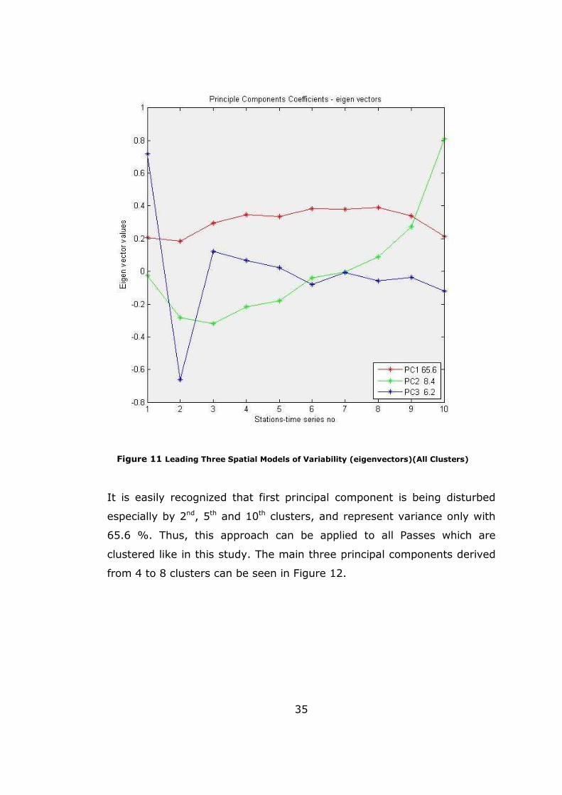
It is easily recognized that first principal component is being disturbed

especially by 2nd, 5th and 10th clusters, and represent variance only with

65.6 %. Thus, this approach can be applied to all Passes which are

clustered like in this study. The main three principal components derived

from 4 to 8 clusters can be seen in Figure 12.

Figure 11 Leading Three Spatial Models of Variability (eigenvectors)(All Clusters)

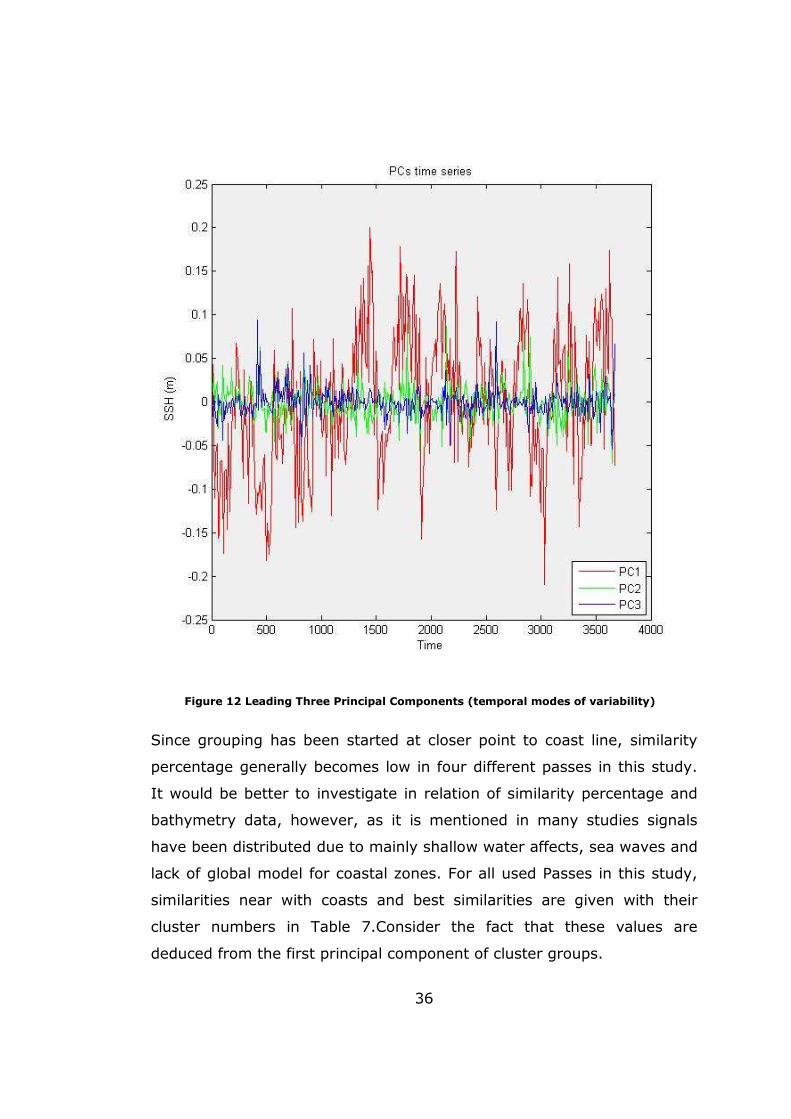
36

Since grouping has been started at closer point to coast line, similarity

percentage generally becomes low in four different passes in this study.

It would be better to investigate in relation of similarity percentage and

bathymetry data, however, as it is mentioned in many studies signals

have been distributed due to mainly shallow water affects, sea waves and

lack of global model for coastal zones. For all used Passes in this study,

similarities near with coasts and best similarities are given with their

cluster numbers in Table 7.Consider the fact that these values are

deduced from the first principal component of cluster groups.

Figure 12 Leading Three Principal Components (temporal modes of variability)

37

Table 7 Most Similar and Coast Cluster Data Groups

According to similarity percentage, a group of five clusters has been

chosen to extract SSH trends from the most similar one group clusters.

Herein, only the trends of Pass 159 are given to see SSH trends and

similarity percentage together. Through Chapter 5, SSH trends from

altimetry missions and SLH trends from tide gauges will be investigated

in detail. To illustrate, the figure of Pass 159 clusters is shown in Figure

13. Note that clusters which are used to extract SSH trend are rounded

with red circle in the figure below.

Pass Number Clusters Percentage

68 (at the coast) 27 - 31 65.88 68 (most similar) 03 – 07 86.61 159 (at the coast) 06 - 10 76.28 159 (most similar) 04 - 08 84.60 170 (at the coast) 31 – 35 65.27 170 (most similar) 03 – 07 90.28 246 (at the coast) 24 – 28 69.66 246 (most similar) 04 – 08 86.60

38

SSH linear trends are deduced from regression analysis of SSH data sets

in each cluster. Significance test of trend parameters and SSH trends can

be seen in Table 8.To sum up, the SSH trends of each Pass are arithmetic

mean of chosen clusters.

Figure 13 All Clusters of Pass 159

39

Table 8 SSH Trends and Test Values of Pass 159

As it is seen in Table 8, from the similarity percentage of PCA method,

the clusters from 4 to 8 (bold in table 8) are used in extracting trends of

SSH to compare with İskenderun Tide Gauge SLH trend. Thus, SSH trend

is found as +8.02 mm/yr with ±1.5 standard deviation for Pass 159 from

Jason-1 and T/P data set. Also, trend value definedwith linear regression

from first principal component of chosen group is +8.04 ±1.3 mm/yr.

Since further results and comments will be mentioned in Chapter 5, only

for Pass 159 altimetry trends are given in this Chapter. To analyze SLH

from tide gauge observations, brief information about tide gauges and

analysis methods are emphasized in the next chapter. Then, daily and

monthly MSLs are computed for seeing SLH trends in Antalya, Bodrum,

Erdemli and İskenderun Tide Gauges.

Note that all other Passes have been processed with the same procedure. The results of each passes can be seen in appendices part of this study.

Cluster

Number

SSH

Trend (mm)

STD. of Trend

Parameter (mm)

T Test Value

(must be >1.28)

1 + 2.3 ± 1.3 1.77 2 + 4.4 ± 1.3 3.45 3 + 6.8 ± 1.4 3.80 4 + 8.4 ± 1.4 4.84

5 + 7.2 ± 1.4 5.22 6 + 9.2 ± 1.4 6.32 7 + 8.8 ± 1.5 5.94

8 + 8.1 ± 1.5 5.30 9 + 6.0 ± 1.5 4.05

10 + 2.4 ± 1.5 1.66

40

CHAPTER 4

4.TIDE GAUGE DATA and PROCEDURE

4.1 Introduction

Sea level variation has been observed by means of tide gauge

measurements gathered over the last century.A tide gauge is

aninstrument for measuring sea levelrelative to the ground. Tide gauges

may also move vertically with the region as a result of post-glacial

rebound, tectonic uplift or crustal motion. This enormously sophisticates

the matter of describing SLHvariationfromtide gauge data. GPS obtains

absolute verticaltrend information so that the sea level data of tide

gauges can be defined at the same reference system with satellite

altimetry, then it is possible to compare tide gauge and altimetry data

directly (IOC 2000).

Differences in SLH estimates from tide gauge data express the need to

account for vertical crustal movements. Tide gauges are exposed

tometeorological influences acting on SLHs like barometric pressure and

wind speed. These variables can be removed from long-term evaluations

of SLH change (Colorado University SLR 2011). Not only tide gauge data

has been used in definition of ocean currents, but also it has been very

useful tool to define long term sea level changes. Specifically, tide gauge

data are in service to describe vertical datum and vertical crustal motion

as an application of geodesy (Yıldız, et al. 2003). A schematic represent

41

of tide gauge is given in Figure 14 (Colorado University SLR 2011),

(JCOMM 2006).

The tide gauge data must be carefully calibrated, checked and evaluated.

The measurements should be connected to local benchmarks which are

fixed into national leveling network and then fixed into the global network

by means of modern geodetic techniques. The recorded data need to be

archived, documented and protected for future studies. Afterwards data

can be considered as a valuable resource and can be used for studies

ranging from local engineering projects to long-term global climate

change (JCOMM 2006). Tide gauges can be split into three parts

according to measurement instrument. These are acoustic gauges with

sounding tubes, pressure sensor tide gauges and stilling well gauges.

Acoustic gauges with sounding tubes form the basis of Turkish Sea Level

Monitoring Network (H. Yıldız 2001).

4.2 Products of A Tide Gauge

Sea level variations can be measured by tide gauge data. These

measurements are in service in a wide range of application areas which

Figure 14 A Tide Gauge Measurement System

(Colorado University SLR 2011)

42

aredetailed in following table, Table 9 (Yıldız, et al. 2003), (Carrera and

Vanicek 1985), (ESEAS 2001).

Table 9 Application Areas of Tide Gauge Data

The effects causing the variation of sea level variations are

meteorological effects, oceanographic effects, tides, climate change and

vertical crustal motion.

At the level of preprocessing of tide gauge data, some software can be

used to tie sea level measurements to a reference point, detection of

time and datum bias with the aid of graphical support, fulfill the short

Application Area Explanations Geodesy • Definition of vertical datum

• Enhancing the precision of vertical control network

• Control of geoid to define gravity

• Definition of vertical land motion

• Definition of post-seismic and Pre-seismic activities

Oceanography, Climatology, Geophysics, Geology,

Meteorology

• Definition of sea slope for estimation of ocean circulation

• Calibration of satellite altimetry measurements

• Geological researches • Climate change

Water Resource Management • Input to define mixture of fresh water and sea water

Hydrology, Hydrography • Correction of lead measurements

• Definition of subsidence transfer roads

• Harbor design Shipping • Sea Navigation

• Guidance of shipping Human and Environmental Security, Saving Coastal

Areas

• Warning and prediction of storms

• Design of protection set

(Yıldız, et al. 2003)

43

gaps. There are three generally known software to use sea level

measurements properly; SLPRC, TASK and FIAMS. These tools utilize to

predict tide analysis, realize quality control and perform filtering (Yıldız,

et al. 2003).

4.3 Tide Gauge Data

In this study, four tide gauges hourly data have been used to analyze sea

level trends. These tide gauges are Antalya, Bodrum, Erdemli,

İskenderun. The detailed information about time interval and geodetic

coordinates are shown in Table 10.

Table 10 Used Tide Gauge Data

Station Name Time Interval (hourly)

Position (lat,lon)

Antalya 2003.1-2010.12 36.8285,30.6093 Bodrum 2003.1-2010.12 37.0323,27.4235 Erdemli 2003.5-2010.12 36.5634,34.2550 İskenderun 2004.12-2010.12 36.5932,36.1802

Not only all hourly data have been given with outlier detected, but also all error sources were classified by data service provider, GCM. To illustrate, a sample of obtained data format is shown in Figure 15.

44

First column shows Date and Time of observation, second column is its

decimal year, third column is for SLH observation at that time, and fourth

one is to give error classification value, data flag. Data Flag number

changes in range from 0 to 9. Zero data flag value means that no quality

control has been made on that value, 1 is for correct value. See the Table

11 for all data flag numbers and their meanings.

Figure 15 A Sample of Hourly TG Data Format

45

Table 11 Hourly Data Flags for Error Classification

Data Flag Value Explanation of Data Flag Value

0 No quality control 1 Correct value 2 Interpolated value 3 Doubtful value 4 Isolated spike or wrong value 5 Correct but extreme value 6 Reference change detected 7 Constant values for more than a defined time

interval 8 Out of range 9 Missing value

Due to already having classified data on the basis of outlier detection, the next step, a classical harmonic analysis of hourly data process has been performed on data.

4.4 Harmonic Analysis on Tide Gauge Data

As mentioned in Introduction Chapter, There are five main factors

affecting on sea level heights like meteorological surges, oceanographic

effects, tidal effects, climate changing, vertical crustal motion. To figure

out periodical tidal effects on sea level heights in each tide gauges, tidal

constituents must have been defined for these four tide gauges. After

giving general information, used tidal harmonic analysis has been

explained below.

Tides are the periodic sea level variations existing due to the combined

effects of the gravitational forces.These forces exist mainly due to the

moon, the sun and the rotation of the Earth. To observe the tide, the

height of sea level is measured as a function of time with respect to a

reference level. The tidal heights and characteristics change with their

location and meteorological conditions. The range of a tide can vary from

ten meters to a few milimeters (Chen and Lee 2001).

Some places on the open sea are exposed to two high and two low tides

each day,semi-diurnal tide, but some locations are only one high and one

46

low tide each day, diurnal tide. The times and amplitude of the tides at

the coast are affected by the incursion of the sun and moon, by the

shape of the coastline and by the sample of tides in the deep ocean and

at near coast bathymetry (Reddy and Affholder 2002), (Hubbard 1997).

Tidal changes are the result of some periodical influences acting in

different frequencies and amplitudes. These influences are known as tidal

constituents. The main constituents are due to the Earth's rotation, the

positions of moon and the sun with respect to Earth, altitude of the moon

above the Earth's equator, and bathymetry. Indeed, tidal forces act on

whole Earth greatly, however, movement of the Earth is only in

centimeters because of solid structure of the Earth.

Since tidal consituents on each tide gauges have different kind of periods

and amplitudes, tidal analysis must be done for each tide gauges

seperately. After performing tidal analysis, predicted signal can be used

in fulfilling gapped data for desired epoch. Primary tidal constituents are

given in Table 12.

47

Table 12 Primary Tidal Constituents

Tidal

Component

Period

(Solar

Hours)

Description Nature

M2 12.42 Principal Lunar Semi-diurnal

S2 12.00 Principal Solar Semi-diurnal

N2 12.66 Large Lunar

Elliptic

Semi-diurnal

K2 11.97 Luni-solar Semi-diurnal

K1 23.93 Luni-solar

Diurnal

Diurnal

O1 25.82 Principal Lunar

Diurnal

Diurnal

P1 24.07 Principal Solar

Diurnal

Diurnal

Q1 26.87 Large Lunar

Elliptic

Diurnal

MF 327.90 Lunar

Fortnightly

Long term

MM 661.30 Lunar Monthly Long term

SSA 4383.00 Solar Semi

Annual

Long term

Tide gauges hourly data for each station have been analyzed for fulfilling

data gap, and also for extracting tidal constituents. For this process, a

classical tidal harmonic analysis approach has been implemented in

hourly data. To perform tidal harmonic analysis, the classical tidal

harmonic analysis including error estimates has been used by means of

T_Tide.m program in MatLab (Pawlowicz, Beardsley and Lentz 2002).

The function of harmonic analysis is:

��8 � �� � P�8 � ∑ g� ����9� � ����� �9� ���….� (4.1)

48

Herein, t is measurement time, x(t) is hourly sea level of timed^�, �� is mean sea level at first epoch, �� is yearly mean sea level trend, N is the

number of tide constituents, �� is frequency of tidal constituent, _�and C�

are the coefficients of tidal constituent’s amplitude. Thus, with the known

frequency, the amplitude of tide gauge can be calculated from equation

4.2.

�8 � �g�Q � ��Q (4.2)

and phase angle from

�^ � W�`dWX ��n� (4.3).

By means of tidal analysis method, tidal constituents are extracted for

each station, note that d is for considered tidal consituent number. Then,

significance amplitudes have been defined with respect to Signal-to-noise

ratio (SNR) value. Tidal constituents which have SNR value greater than

2, is taken into account to get predicted signal for each station.

SNR is defined as the ratio of signal power to the noise power. It is seen

that if SNR value is equal or bigger than 2predicted values are consistent

to each other. This fact results from comparison of parametric bootstrap

and SNR.It is suggested that if a tidal constituent has lower than 2 SNR

value, the tidal constituent should not be performed in the process of

getting predicted value (Pawlowicz, Beardsley and Lentz 2002).

Significant tidal constituents and their SNR values for Erdemli station

(2003-2010) are shown in Table 13.

49

Table 13 Significant Tidal Constituents of Erdemli Station (2003-2010)

Standard deviation of difference between input hourly data and hourly

data obtained from predicted signal is ±9.10 cm for Erdemli Station. See

relevant standard deviations for all stations used in this study in Table

14.

Tide Frequency

(1/hour)

Amplitude

(m)

Amp.

Error(m)

Phase

(deg)

Phase

Error

(deg)

SNR

SA 0.0001141 0.1057 0.013 229.95 6.64 65 SSA 0.0002282 0.0303 0.012 261.16 23.29 6.5 Q1 0.0372185 0.0028 0.001 242.40 10.19 30 O1 0.0387307 0.0193 0.000 256.08 1.35 1.7e+003 NO1 0.0402686 0.0013 0.000 253.20 18.01 12 PI1 0.0414385 0.0011 0.001 233.46 30.83 3.5 P1 0.0415526 0.0099 0.001 284.79 3.89 2.8e+002 S1 0.0416667 0.0086 0.001 246.71 5.05 1.1e+002 K1 0.0417807 0.0273 0.001 277.57 1.12 2.6e+003 PSI1 0.0418948 0.0015 0.001 173.71 22.40 6.9 J1 0.0432929 0.0014 0.001 266.67 21.70 6.9 OO1 0.0448308 0.0009 0.000 245.34 16.94 9.3 N2 0.0789992 0.0178 0.002 230.21 6.98 77 NU2 0.0792016 0.0032 0.002 228.32 37.53 2.4 H1 0.0803973 0.0047 0.002 302.05 24.52 4.9 M2 0.0805114 0.1068 0.002 228.97 1.18 2.2e+003 H2 0.0806255 0.0058 0.002 142.89 19.23 8.4 L2 0.0820236 0.0054 0.003 212.41 29.56 3.9 T2 0.0832193 0.0036 0.002 203.91 31.62 3.3 S2 0.0833333 0.0615 0.002 244.00 1.99 9.7e+002 K2 0.0835615 0.0172 0.001 241.72 5.30 1.4e+002 MSN2

0.0848455 0.0004 0.002 48.95 189.19 0.062

MO3 0.1192421 0.0007 0.000 33.13 19.73 11 M3 0.1207671 0.0026 0.000 1.44 5.15 1.1e+002 SO3 0.1220640 0.0003 0.000 84.46 48.86 1.7 MK3 0.1222921 0.0001 0.000 28.12 80.03 0.57 SK3 0.1251141 0.0010 0.000 294.90 12.84 21 M4 0.1610228 0.0007 0.000 292.94 12.99 28 MS4 0.1638447 0.0005 0.000 325.36 18.01 13 MK4 0.1640729 0.0002 0.000 325.40 30.87 4.4 2SK5 0.2084474 0.0001 0.000 282.55 40.98 2.2

50

Table 14 Standard Deviation of Difference in Original & Predicted Data

To define tidal constituents more conveniently, there must be hourly tide

gauge data for 18.6 years. Because, the significant tidal constituent

which has the longest term period covers 18.6 years (H. Yıldız 2001). In

this study, because of having less time span to seperate tidal

constituents in each station, some long term tidal constituents have not

been defined in data set (Yıldız, et al. 2003). Then, as it can be seen from

the Table 13, standard deviation of difference between actual data and

predicted data becomes lower rationally with measurement time span.

Note that standard deviation occurs due to huge data gaps in actual data

as well.

After extracting tidal constituents and getting predicted signal in each

station for data gaps, filtering operation has been made to see daily and

monthly mean sea level of each station.

4.5 Filtering of Hourly Data

As mentioned above, filtering is required to define mean sea levels firstly

on the basis of daily, and secondly on the basis of monthly. SLPR2

program which is developed by cooperatin of University of Hawaii The

Tropical Ocean Global Atmosphere Program Sea Level Center and the

USA National Oceanographic Data Center has been used to calculate

mean sea levels (TOGA tarih yok).

Tide Gauge Station Time Span Standard Deviation

(cm)

Antalya 2003.1-2010.12 ±8.96

Bodrum 2003.1-2010.12 ±8.29

Erdemli 2003.5-2010.12 ±9.10

İskenderun 2004.12-2010.12 ±10.37

51

Program provides daily values from hourly data in two steps:

• Diurnal and Semi-diurnal components are removed

• To remove remaining high frequency, a 119-point low pass filter is

applied.

Note that daily mean sea level can be calculated if there is a data gap

less than 24 hours in hourly data. Outputs of predicted signal can be

used to fulfill these considered data gaps. Therefore, monthly mean sea

level data has been calculated from simple arithmetic mean of daily mean

sea level. Also, if there is a gap of daily mean sea level data set covering

more than seven days, related monthly mean sea level has not been

calculated (Yıldız, et al. 2003).

In this aspect, filtering application has been made for all stations. Then,

monthly mean sea levels have been compared with PSMSL monthly sea

levels. It is seen that monthly mean sea level extracted from SLPR2

software by means of filtering hourly data was consistent with PSMSL

monthly mean sea level data. Also, some data gaps existing in PSMSL

data set has been fulfilled from calculated data set. Note that Table 15

includes PSMSL monthly mean sea level and calculated mean sea level

between at the year 2009for Erdemli tide gauge.

52

Table 15 Calculated & PSMSL MSL for Erdemli, 2009

Month Calculated Monthly MSL (m)

MSL from PSMSL (m)

1 1.008 1.008 2 1.181 1.181 3 1.096 1.095 4 1.086 1.084 5 1.105 1.105 6 1.214 1.214 7 1.306 1.306 8 1.275 1.275 9 1.256 1.257

10 1.203 1.203 11 1.233 1.233 12 1.306 1.306

It is mentioned that for data gap first of all the difference between

predicted values and calculated values have to be computed. Then, for a

gapped data time, the closest data must have been defined to apply

linear interpolation for gapped time. Lastly, linear interpolation value

must be added to predicted value. Note that this method is valid for less

than 24 hour data gaps. Due to data consistency of MSL between PSMSL

data and calculated data, predicted hourly values have been used directly

to fulfill PSMSL data gaps in this study. Additionally, because of

consistency between calculated and provided by PSMSL data set, PSMSL

monthly mean sea level values have been used to extent monthly mean

sea level data set. So that it is made possible using PSMSL MSL data set

to see the SLH trends of each station.

Note that data gaps included in PSMSL data set has been fulfilled by

calculated MSL values. To illustrate, PSMSL data set Antalya 2006 has no

value in any month, but all the values of considered month are calculated

by means of predicted values. Results can be seen in Table 16. The value

of ‘9999’ means that there is no MSL value for relevant month.

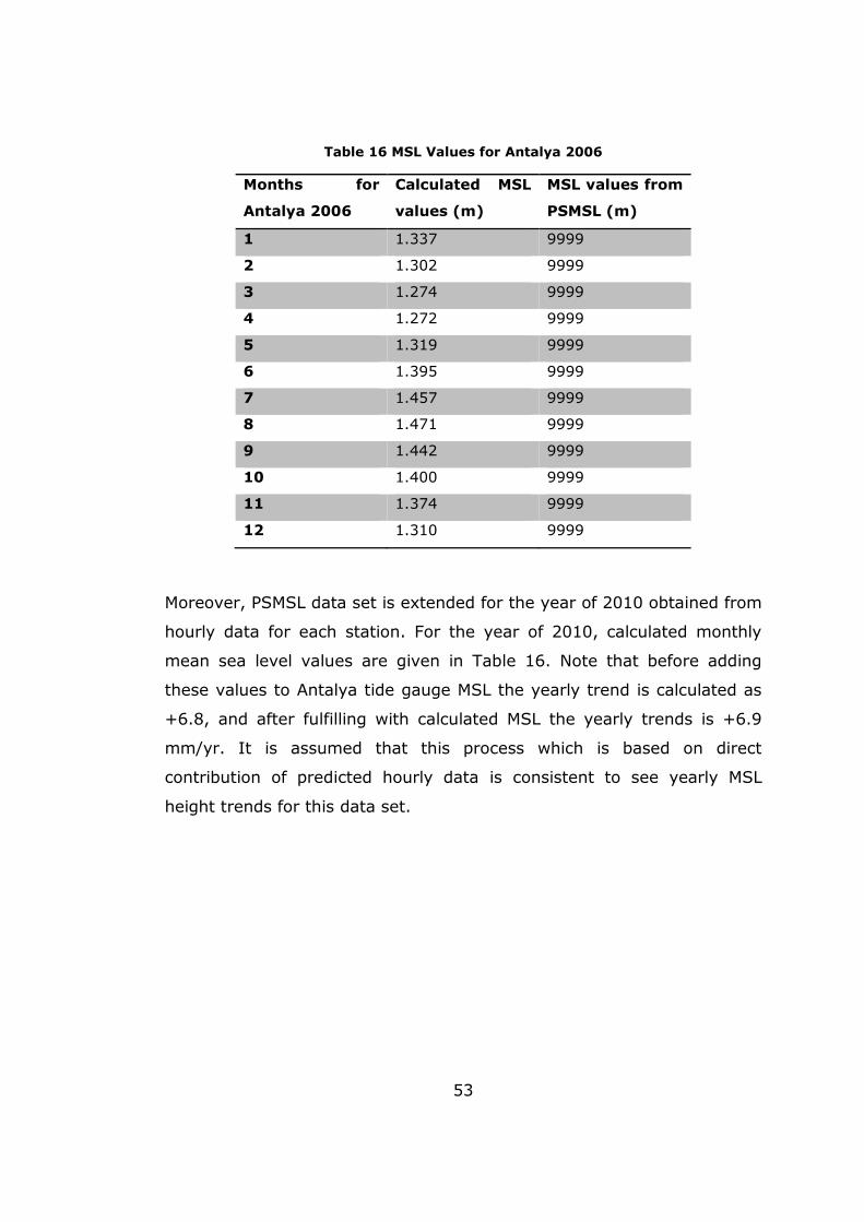
53

Table 16 MSL Values for Antalya 2006

Months for

Antalya 2006

Calculated MSL

values (m)

MSL values from

PSMSL (m)

1 1.337 9999

2 1.302 9999

3 1.274 9999

4 1.272 9999

5 1.319 9999

6 1.395 9999

7 1.457 9999

8 1.471 9999

9 1.442 9999

10 1.400 9999

11 1.374 9999

12 1.310 9999

Moreover, PSMSL data set is extended for the year of 2010 obtained from

hourly data for each station. For the year of 2010, calculated monthly

mean sea level values are given in Table 16. Note that before adding

these values to Antalya tide gauge MSL the yearly trend is calculated as

+6.8, and after fulfilling with calculated MSL the yearly trends is +6.9

mm/yr. It is assumed that this process which is based on direct

contribution of predicted hourly data is consistent to see yearly MSL

height trends for this data set.

54

Table 16 Monthly MSL Values, 2010

Tide Gauge Month Calculated Monthly MSL (m)

Antalya

1 1.473 2 1.460 3 1.352 4 1.292 5 1.365 6 1.468 7 1.479 8 1.537 9 1.523 10 1.440 11 1.458 12 1.528

Bodrum

1 1.327 2 1.330 3 1.342 4 1.272 5 1.329 6 1.420 7 1.396 8 1.450 9 1.453 10 1.427 11 1.449 12 1.512

Erdemli

1 1.256 2 1.221 3 1.146 4 1.086 5 1.164 6 1.277 7 1.284 8 1.326 9 1.327 10 1.240 11 1.232 12 1.325

İskenderun

1 2.269 2 2.245 3 2.180 4 2.190 5 2.220 6 9999 7 9999 8 9999 9 2.372 10 2.288 11 2.274 12 2.303

55

Since the provided data has not measurement epoch at the months

properly, sixth, seventh,eigth MSL values of İskenderun for 2010 have

not MSL value. If measurement epochs would have been entered even

with NaN (Not-a-Number) value, prediction values of these three months

would be calculated.

Before getting through determining vertical trends chapter, processes can

be summarized until this point. Firstly satellite altimetry measurements

are clustered, detected against with outlier, trend parameters are tested,

outlier methods have been compared, data gaps have been fulfilled on

the basis of time and frequency domain. Then, PCA analysis has been run

to see the similarity and differences in each cluster for used passes.

On the other hand, hourly tide gauge data was detected for outlier by

data provider, GCM. Then, to define tidal constituents and fulfill data

gaps of hourly sea level data, harmonic analysis has been made for each

station. Therefore, It is possible to calculate daily and monthly MSL for

each station.

To get more confident vertical trends from comparison of tide gauge and

altimetry data, Global Positioning System (GPS) trends must be taken

into account. However, as will be mentioned at the next chapter, there

are some drawbacks to use GPS observations confidently.

56

CHAPTER 5

5. DETERMINING VERTICAL TRENDS

This chapter basically covers the trends of SSH from satellite altimetry

and SLH from tide gauge observations. Although GPS trends are given by

data provider, GCM, GPS campaigns cause some drawbacks to see

vertical motion of crust directly. Therefore, GPS measurement epochs will

be handled with explanations on the evaluating process of vertical

motions.

5.1 Trends From Tide Gauges and Altimetry Satellites

As mentioned at the beginning, SLH trends deduced from tide gauges,

mixed with crustal motion. Thus, it is needed to seperate this mix by

means of external absolute observations like SSH derived from satellite

altimetry.

To define the trends of tide gauges harmonic analysis has been applied to

monthly MSL of each tide gauges. This harmonic analysis can be

represented as

�$ � _� � ∑ g�cos ���8$ � ø� q¡�� (5.1)

M constituents to be included in the analysis. As unknowns _¡ andø¡are

amplitude and phase of constituent, ¢¡ is frequencyof constituent, T is the measured SLH,A� is averagesea level trend, i is the observation time,

j is the number of constituents.

Also, frequencies as an input parameter can be seen in Table 17.

57

Table 17 Used frequencies for SLH Trends

In the process of defining SLH trends, significance of trend parameters

has been tested with T test value. A frequency which has been found

insignificant according to trend parameters, has been removed from input

folder. Then, harmonic analysis has been started to be calculated from

scratch. This process has been continued till finding at least one

parameter of each retained constituent significant.

Moreover, linear regression analysis has been applied to the monthly MSL

of each tide gauges. Trends computed from linear regression analysis and

harmonic analysis are shown in Table 18.

Frequency Number Frequency (1/month) Period (Month)

1 0.0089559 111.6582 2 0.0233175 42.8862 3 0.0739339 13.5256 4 0.0788574 12.6811 5 0.0833281 12.0008 6 0.0878061 11.3887 7 0.1433533 6.9758 8 0.1478313 6.7645 9 0.1572547 6.3591

10 0.1666709 5.9998 11 0.1711489 5.8429 12 0.1756268 5.6939 13 0.249999 4.0000 14 0.254477 3.9296 15 0.3333344 3.0000 16 0.8689882 1.1508 17 0.8734662 1.1449 18 0.929006 1.0764 19 0.9334768 1.0713 20 0.9473782 1.0555 21 0.9523163 1.0501 22 0.9567943 1.0452 23 0.9612723 1.0403

58

Table 18 SLH Trends from Tide Gauge Observations

Although the trends from linear regression and harmonic analysis are

similar to each other, the trends from harmonic analysis are more

appropriate for SLH nature. Since each tide gauge has different tidal

constituents, significant constituents must be defined specially for each

tide gauges. The difference of constituentsis taken into account by

means of harmonic analysis process. Thus, to compare with altimetry

vertical trends, the trends of harmonic analysis on MSL will be used in the

process of extracting vertical trends and vertical crustal motions.

As mentioned before, vertical trends from altimetryobservations are

defined from arithmetic mean of linear regression of chosen clusters. To

remind, clusters have been chosen with respect to their similarity

percentage. See Table 19 for vertical trends from altimetry observations.

Table 19 SSH Trends from Altimetry Observations

Pass Number

Chosen Clusters

Similarity Percentage

Trends (mm/yr)

68 03 – 07 86.61 + 5.8 ± 1.5 159 04 – 08 84.60 + 8.0 ± 1.5 170 03 – 07 90.28 + 9.5 ± 1.3 246 04 – 08 86.60 + 8.3 ± 1.5

After considering the trends from GPS, comparison of vertical trends will

be made in this chapter at the last section. As the next step, GPS trends

will be defined and investiaged in each station.

Tide Gauge

Trend (mm/yr) Linear Regression Harmonic Analysis

Antalya + 7.2 ± 0.6 + 6.9 ± 0.4 Bodrum + 3.3 ± 0.6 + 3.3 ± 0.6 Erdemli + 6.6 ± 4.7 + 7.9 ± 2.9 İskenderun + 59.6 ± 6.0 +57.4 ± 3.3

59

5.2 GPS Solution

The Global Positioning System (GPS) is a satellite positioning and

navigation system that ensures time and locationinformation on or near

the Earth. Note that there must be at least 4 GPS satellites in view to

define position. It is maintained by the USA, and is available for anyone

who has a GPS receiver. But there are some technical limitations which

are only in use for military users.

To explain basically, the satellite is continually marked with own

transmission time so that when received the signal transit period can be

measured with a synchronized receiver. The original objectives of GPS

were the instantaneous determination of position and velocity, and the

precide coordination of time (Hofmann Wellenhof, Lichtenegger and

Wasle 2008), (Chen and Lee 2001). Since there is a wide range of

information about GPS technique at different resources, detailed

information will not be given in this study.

Used GPS velocities have some drawbacks to use in comparison process

of vertical crustal motion. First one, the GPS velocities are not derived

from continuously operated observations. Latter one is that GPS

campaigns are not regular and do not cover observation years of neither

tide gauges, nor satellite altimetry. For some of tide gauges, GPS

observations have been done from the point which is not on the tide

gauge. It is realized as another disadvantage of GPS observations. Thus,

GPS vertical trends will be evaluated seperately on the process of

extracting vertical motion. The GPS campaigns which isused to derive

coordinate velocities can be reached in Table 20.

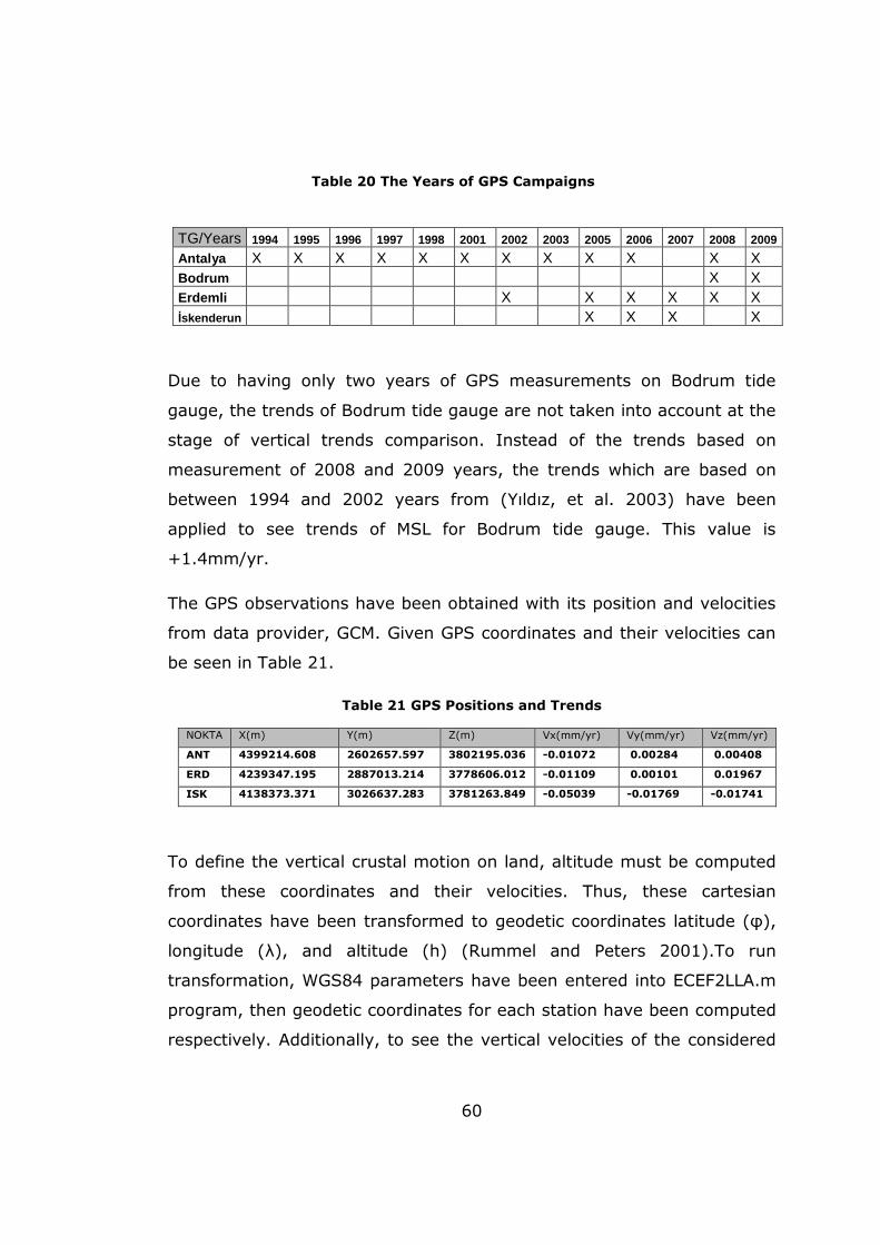
60

Due to having only two years of GPS measurements on Bodrum tide

gauge, the trends of Bodrum tide gauge are not taken into account at the

stage of vertical trends comparison. Instead of the trends based on

measurement of 2008 and 2009 years, the trends which are based on

between 1994 and 2002 years from (Yıldız, et al. 2003) have been

applied to see trends of MSL for Bodrum tide gauge. This value is

+1.4mm/yr.

The GPS observations have been obtained with its position and velocities

from data provider, GCM. Given GPS coordinates and their velocities can

be seen in Table 21.

Table 21 GPS Positions and Trends

NOKTA X(m) Y(m) Z(m) Vx(mm/yr) Vy(mm/yr) Vz(mm/yr)

ANT 4399214.608 2602657.597 3802195.036 -0.01072 0.00284 0.00408

ERD 4239347.195 2887013.214 3778606.012 -0.01109 0.00101 0.01967

ISK 4138373.371 3026637.283 3781263.849 -0.05039 -0.01769 -0.01741

To define the vertical crustal motion on land, altitude must be computed

from these coordinates and their velocities. Thus, these cartesian

coordinates have been transformed to geodetic coordinates latitude (φ),

longitude (λ), and altitude (h) (Rummel and Peters 2001).To run

transformation, WGS84 parameters have been entered into ECEF2LLA.m

program, then geodetic coordinates for each station have been computed

respectively. Additionally, to see the vertical velocities of the considered

TG/Years 1994 1995 1996 1997 1998 2001 2002 2003 2005 2006 2007 2008 2009

Antalya X X X X X X X X X X X X Bodrum X X Erdemli X X X X X X İskenderun X X X X

Table 20 The Years of GPS Campaigns

61

tide gauges, velocities given in cartesian coordinates have been

translated into geodetic coordinates, WGS84.

The translation has been made by means of the formula below (Torge

2001)

� � g��¤� (5.2)

Hereby,

g�� =¥�bEXφcosλ �sinφsinλ `abφ�bEXλcosφcosλ `abλcosφsinλ 0bEXφ ª (5.3)

And,

ΔΔΔΔX = t2t¬t­ (5.4).

Resulted velocities can be seen in Table 22.

Table 22 GPS Velocities

Tide Gauge ∆φ (mm/yr) ∆λ (m/yr) ∆h (m/yr)

Antalya +7.9 +7.9 -3.8

Erdemli +20.9 +7.1 +4.8

İskenderun +16.5 +15.5 -51.4

As it is seen from the Table 21 except for Antalya tide gauge, the tide

gauges used in this study have huge amount of gaps. The comparison of

vertical trends has been made at the next section of this chapter.

5.3 Determination of Sea Level Trends and Vertical Land Motions

Following the procedure explained through this study thus far, differential

sea level trends between tide gauges and altimetry observations are

calculated. Also, GPS trends have been considered seperately to see

62

vertical motions in each stations. Relevant results have been shown in

Table 23.

63

Table 23 Comparison of Vertical Trends

(a) SSH Trends obtained from the most similar group of clusters

Pass No.

Station Satellite Altimetry (ALT) Tide Gauges (TG) ALT-TG (mm/yr)

GPS Solution Trend (mm/yr)

ALT- (TG+GPS) (mm/yr)

Time Span Trend(mm/yr) Time Span Trend(mm/yr)

246 Antalya 1999.1-2009.1

+ 8.3 ± 1.5 1985.11-2010.12

+ 6.9 ± 0.4 +1.4 -3.8 + 5.2

170 Bodrum 1999.1-2009.1

+ 9.5 ± 1.3 1985.12 – 2010.12

+ 3.3 ± 0.6 +6.2 +1.4 +4.8

68 Erdemli 1999.1-2009.1

+ 5.8 ± 1.5 2003.1-2010.12

+ 7.9 ± 2.9 -2.1 +4.8 -6.9

159 Iskenderun 1999.1-2009.1

+ 8.0 ± 1.5 2005.1-2010.12

+57.4 ± 3.3 -49.4 - 51.4 +2.0

Mean -11.0 -12.3 +1.3

63

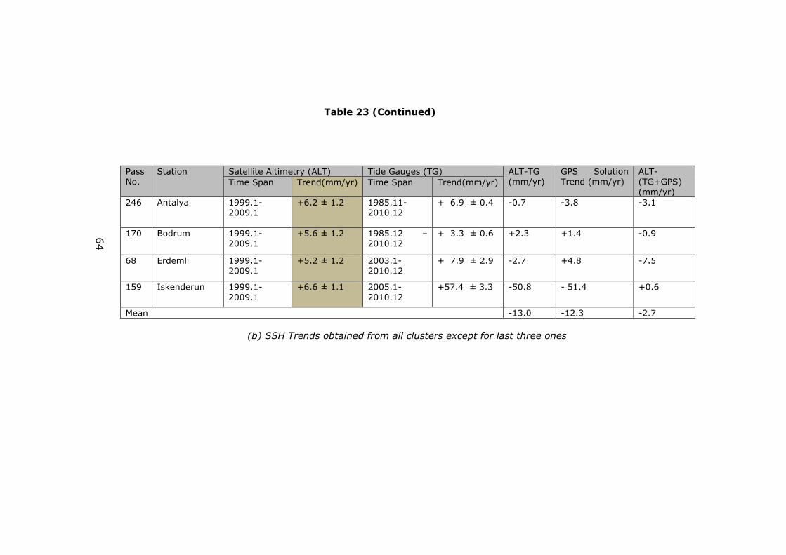
64

Table 23 (Continued)

(b) SSH Trends obtained from all clusters except for last three ones

Pass No.

Station Satellite Altimetry (ALT) Tide Gauges (TG) ALT-TG (mm/yr)

GPS Solution Trend (mm/yr)

ALT- (TG+GPS) (mm/yr)

Time Span Trend(mm/yr) Time Span Trend(mm/yr)

246 Antalya 1999.1-2009.1

+6.2 ± 1.2 1985.11-2010.12

+ 6.9 ± 0.4 -0.7 -3.8 -3.1

170 Bodrum 1999.1-2009.1

+5.6 ± 1.2 1985.12 – 2010.12

+ 3.3 ± 0.6 +2.3 +1.4 -0.9

68 Erdemli 1999.1-2009.1

+5.2 ± 1.2 2003.1-2010.12

+ 7.9 ± 2.9 -2.7 +4.8 -7.5

159 Iskenderun 1999.1-2009.1

+6.6 ± 1.1 2005.1-2010.12

+57.4 ± 3.3 -50.8 - 51.4 +0.6

Mean -13.0 -12.3 -2.7

64

65

CHAPTER 6

6. RESULTS

6.1 Discussion on Trend Progress

In this study, SSH trends, SLH trends and GPS vertical crustal trends

have been compared with each other. The study shows that altimetry and

tide gauge vertical trends are coherent to each other, and give vertical

positive trends for Mediterranean coast of Turkey. This means that sea

level is rising every year more or less 7 mm at the Mediterranean coast

of Turkey.

It is required to mention that even though GPS trends have been used to

understand vertical land motion in the study area, these values are not

reliable due to only having velocities rather than observations. Also, the

method which is used to extract SLH trends from tide gauges is accepted

as appropriate one, however, time span of data collection is not quite

enough to use harmonic analysis method due to not being revealed long

term periods. It is suggested that there must be at least a decade of MSL

values for a tide gauge, however, İskenderun and Erdemli Tide Gauges

do not have at least a decade of time span.

As it is mentioned in related part of this study, data gaps of tide gauges

have been fulfilled by means of hourly outputs of predicted signal values

because of monthly existing MSL consistency between PSMSL data and

calculated MSLs. However, it is suggested that for data gap first of all the

difference between predicted values and calculated values must be taken.

Then, for a gapped data time, the closest data must have been defined to

66

apply linear interpolation for gapped time. Lastly, linear interpolation

value must be added to predicted value. Note that this method is valid

for less than 24 hour data gaps.

For altimetry measurements, PCA similarity approach has been used to

see SSH trends. This method is a kind of useful approach to see common

behavior of SSH trendsgroup by group. Moreover, it gives an advantage

to work on shallow water for SSH trends due to showing similarity of

each clusters which are collected in a group.

On the other hand, using a group of five clusters decreases the

measurements which have been obtained from altimetry missions. To

illustrate, for Pass 68, there are available 10850 observations extracted

from the missions, but only chosen 1750 observations have been used to

define SSH trends in Table 23 (a). This situation is due to working in

shallow water areas. Assuming that SSH must be homogenus in 30 km

distance, after getting the most similar group resulted from PCA

method,it can be said that consistent data is available to extract SSH

trends, and in this way, coastal effect on SSH observations are

investigated as well. On the other side, except for last three clusters, all

clusters have been considered to figure out SSH trends for each pass. It

is worthwhile to mention that the SSH trend differences between Table

23 (a) and (b) are mainly due to location difference of used clusters.

GPS velocities can be used to see the vertical motion of crust. However,

these velocities must be obtained from continuous GPS (CGPS)

observations. In this study, because of not having CGPS observations,

there is no statistical investigation in GPS solutions. Therefore, GPS

vertical velocities derivede from Episodic GPS (EGPS) observations have

been evaluated seperately in the process of extracting vertical trends.

67

6.2 Evaluation of the Results

As it is seen from the Table 23 (a) and (b), SSH trends are deviating

from each other mostly 3.8 mm, and 1.4 mm respectively. There are

some reasons acting on SSH trends cause these milimetric trend

differences. These can be summarized as follow

• Meteorological effects like wind, pressure,

• Measurement accuracy,

• Slope of sea,

• Bathymetry,

• Unmodeled instrumental errors,

• Lack of global correction,

• Local salinity and temperature differences.

Besides, SLH trends derived from tide gauges deviates much more than

SSH trends. The main reason is that as the main subject of this study

tide gauges measure sea level, due to being set up on the Earth crust,

they detect both sea surface height variations and vertical crustal

movements. Also, meteorologic observations are required to see the

effect of them on SLH variations.

Although T test results ontrend parameters show that the trends deduced

from Erdemli and İskenderun tide gauges are statistically significant, it is

suggested that tide gauge observations must cover at least a decade to

figure out vertical SLHs confidently. Because of some tidal effects acting

on SLH trends significantly can be extracted by 10 years hourly SLH data.

Thus, these effects must be defined and removed from MSL trends.

For Table 23 (a), looking at Antalya and related Pass, Pass 246,denotes

difference +1.4 mm which means that tide gauge location goes up,

however, GPS solution does not agree with this trend. It can be due to

not having CGPS measurements. Also, if the clusters from 19 to 23 would

be considered to calculate SSH trends which are more closer than used

68

clusters sea level trend would be +3.6 mm/yr. This means that

consistent result would be available with sea level trends deduced from

Antalya tide gauge. However, due to not having the most similar

behavior from these clusters, this result is not put into vertical trend

comparison table. Note that the distance between five clusters which are

used to have SSH trends and Antalya tide gaugeis far by 202 km, can be

a part of reason for that difference. On the other side, Table 23 (b)

represents consistent result with GPS solution. If the vertical trend

deduced from GPS velocity is correct, it can be said that shallow water

acts on SSH observations only 25 km near with coastal side of Antalya

station.

It is seen that tide gauge location moves up +6,2 mm every year with

respect to ALT-TG difference between Pass 170 and Bodrum tide gauge

vertical trends in Table 23 (a). Also, GPS solution shows that there is a

trend equals to +1.4 mm for each year. The results represent

consistency, but there is no considerable vertical movement of Bodrum

station. Considering Table 23 (b) gives more consistent result than the

most similar group approach. In these aspects, it can be confidently said

that the Bodrum station goes up gradually.

As third station, Erdemli is evaluated with Pass 68 of satellite altimetry

missions. For Table 23 (a), SSH has +5.8 mm trend in a year, on the

other hand, Erdemli station gives +7.9 mm value. It is shown that

Erdemli tide gauge decreases in amount of - 2.1 mm each year. But,

EGPS solution shows +4.8 mm trend for Erdemli station. This difference,

like Antalya tide gauge, can be both resulted from distance between

Erdemli station and chosen clusters, and lack of continuous GPS

observations. Also, note that tide gauge observation time span and data

gaps can not give enough outputs to detect vertical crustal motion

confidently. Last but not least thing, some GPS observations instead

being observed on tide gauge point, gathered on a close location to the

tide gauge. Both local crustal movement differences between GPS and

69

tide gauge points and absence of meteorological observations can cause

this dilemma for the trend solution. Note thin Table 23 (b) SSH trends

deduced from altimetry observations give more or less the same result

with Table 23 (a) for Pass 68.

As the last tide gauge, İskenderun station is handled with Pass 159.

Although having only for 6 years observations on İskenderun station, it is

seen that this tide gauge rises sharply. Altimetry observations show the

+8.0 and +5.2 mm trend Table 23 (a) and (b) for each year, however,

İskenderun tide gauge represents +57.4 mm trend. GPS processing

result points that İskenderun tide gauge decreases 51.4 mm in a year.

This means that there is a huge amount of vertical crustal motion for

İskenderun tide gauge. Also, there is a high level consistency on vertical

trends between altimetry, tide gauge and EGPS velocities. This station

must be observed with continuous GPS receiver to detect its velocity

regularly. If it is possible, the tide gauge station can be relocated to the

place where is tectonically less active.

70

CHAPTER 7

7. CONCLUSION AND RECOMMENDATIONS

In this study, SSH derived from altimetry missions have been used to see

sea level variations in space and time. Due to time resolution and time

span of advantage, Jason-1 and T/P missions have been chosen as

reference altimetry satellites. Clustering process was the first step of this

study on altimetry data, as second step quality control has been made by

means of Pope and T test approaches. Then, each observation is

relocated to related center with respect to geoid height difference

between cluster center and measurement positions. To apply PCA

method, each cluster has been analyzed and interpolated as time series

within frequency and time domain methods. Thus, PCA method has been

implemented in time series in each cluster to figure out similarities of

them. Moreover, all clusters except for last three ones have been used to

consider the change of SSH trend values in each Pass as well.

Also, tide gauge data obtained from GCM has been analyzed to reveal

tidal constituents and fulfill data gaps in hourly data. Four stations have

been evaluated which are lengthening at the Mediterranean coast of

Turkey. Then, to extract daily and monthly MSL values of each tide gauge

a 119 point convolution filter has been used to do so. Monthly MSL data

obtained from PSMSL have been fulfilled with calculated MSL values.

Afterwards, SLH trends have been computed by means of both linear

regression and harmonic analysis.

To have more convenient vertical trends EGPS solution has been

considered. So that vertical trends and probable error resources were

71

under inspection to figure out advantages and disadvantages of

considered data and methods.

To select the proper outlier detection method PEB value has been applied

to SSH data. It is seen that Pope outlier test gives dominantly better

results than Interquartile method with respect to PEB value. Also,

relaocating SSHs by geoid height to their centers reduced the standard

deviation of each cluster significantly. To sum up, Pope test as an outlier

detection method and geoid height as reference height to relocate SSH

values are useful tools to implement in SSH values. So that all

measurements are brought to their centers correspondingly.

The future work deduced from this study has been mentioned at the

following part.

Although Jason-1 and T/P has better time resolution than ENVISAT

mission, there is a mission called ENVISAT which has better spatial

resolution than the Jason-1 and T/P. Because of calling for continues

observations covering at least ten years in study area, ENVISAT has not

been chosen as reference altimetry mission in this study. However, two

years later there can be a study to work with ENVISAT for seeing SSH

trends and comparing them with tide gauge observations in the study

area.

To cluster SSH observations, K-means clustering method has been

applied to the data. As mentioned before, cluster numbers have been

entered manually into operation. Thus, clustering process which is based

on K-means method must be automated by developing an algorithm to

define cluster numbers automatically. Also, if cluster numbers become

more than 28, all data must be divided into two parts for K-means

clustering process. There can be study to perform these tasks

automatically.

After application of frequency domain analysis of SSH data set, the

dominant periods have been defined in data. These periods are for 1, 2,

72

6, 8 years, clearly, exact values are available in appendices. So that it

can be said that some local tidal effects which are not extracted by global

ocean tide model (GOT 4.7) can be still existing in corrected SSH

observations for Mediterranean Sea.

Since the study area is known as shallow water, PCA method has been

implemented in data to see common behavior of clusters in time. Also,

bathymetric data can give information to figure out the relation between

cluster similarities and bathymetry. So that proper clusters can be chosen

by means of bathymetry data in this area. Also, to make decision about

sufficient amount of similarity percentage to extract SSH trends can be

defined with further studies. Then, there may be no need to take the best

similar group which is sometimes so far from tide gauge station. In this

aspect, there can be some studies to improve GOT 4.7 for Mediterranean

Sea.

Although four tide gauges have been investigated in this study, some of

which had both an amount of MSL data gap and short time span. It would

be quite well if there would have been continuos observations covering at

least a decade,however, used hourly data do not meet with this

condition.Moreover, Doodson number sets are used to define tidal

constituents from hourly data, instead of this number set, some different

number sets can be applied to the hourly data to get more constituents

and see its effects on SLH trends in each station.As mentioned before,

meteorological measurements must have been taken to model the effects

like wind, pressure etc.

As last but not least thing, there is a service which is called CORS-TR to

perform observations on GNSS satellites. To have continues observations

this system can be used to collect position data of each tide gauge. Also,

GPS observations must be done exactly on the same location of tide

gauges to separate crustal motions from SLH trends precisely.

73

REFERENCES

(SLC), University of Hawaii. Hawaii Uni. http://ilikai.soest.hawaii.edu/UHSLC/jaslsoft2.html (accessed 11 07, 2011).

Allison, Paul D. Logistic Regression Using the SAS System. SAS Institute, 1999.

AVISO. Product. April 2011. ftp://ftp.aviso.oceanobs.com/pub/oceano/AVISO/SSH/monomission/dt (accessed August 30, 2011).

AVISO, Handbook. DT CorSSH and DT SLA Product Handbook. AVISO, 2011.

Ball, G., and D. Hall. “A Clustering Technique for Summarizing Multivariate Data.” Behavioral Science, 1967: 153-155.

Barnett, T.P. "The Estimation of "global" sea level change: a problem of uniqueness." Journal of Geophysical Research, 1984: 7980-7988.

Barnett, V., and T. Lewis. Outliers in Statistical Data. John Wiley & Sons., 3rd edition, 1994.

Benveniste, Jérôme, and Nicolas Picot. Radar Altimetry Tutorial. ESA, CNES, 2011.

Birney, D.S., G. Gonzalez, and D. Oesper. Observational Astronomy. Cambridge University Press, 2006.

Bosch, Wolfgang, and Roman Savcenko. BIN data structure - altimeter

data reorganized for time series analysis. Münich: Deutsches Geodatisches Forschungsinstitut, 2005.

Braitenberg, Carla, Patrizia Mariani, Lavinia Tunini, Barbara Grillo, and Ildiko Nagy. "Vertical Crustal Motions from Differential Tide Gauge Observations and Satellite Altimetry in Southern Italy." Journal of

Geodynamics, 2010.

CalVal, AVISO. AVISO CalVal. 2011. http://www.aviso.oceanobs.com/en/newsstand/newsletter/newsletter07/jason-1-calibrationvalidation/index.html (accessed 11 05, 2011).

Carrera, G., and P. Vanicek. “The Use of Sea Level Tide Gauge Observations in Geodesy.” Lighthouse Edition, 1985: 13-16.

74

Chen, Y.Q., and Y.C. Lee. Geographical Data Acquisition. Wien: Springer-Verlag, 2001.

Colorado University SLR, Sea Level Research Group. 2011. http://sealevel.colorado.edu/content/tide-gauge-sea-level (accessed September 1, 2011).

De Boor, C. A Practical Guide to Splines. Springer, 2001.

Douglas, Bruce C. "Global Sea Level Change: Determination and interpretation." Reviews of Geophysics, 1995: 1425-1432.

eHow. eHow. 2011. http://www.ehow.com/how_4546238_calculating-percentage-error.html (accessed September 1, 2011).

ESA, and CNES. Basic Radar Altimetry Toolbox v3.0 User Manual. ESA, CNES, 2011.

ESEAS. Description of Scientific/Technological Objectives and Work Plan,

Part B, First Draft of Proposal for Support for Research Infrastructure. European Sea Level Service, 2001.

Fu, Lee-Lueng, and Anny Cazenave. Satellite Altimetry and Earth

Sciences. California: ACADEMIC PRESS, 2001.

Garcia, D, I. Vigo, B.F. Chao, and M.C. Martinez. "Vertical Crustal Motion Along the Mediterranean and Black Sea Coast Derived from Ocean Altimetry and Tide Gauge Data." Pure and Applied Geophysics, 2007: 851-863.

Govaert, Gerard. Data Analysis. Wiley, 2009.

Groger, M., and H. Plag. “Estimations of a Global Sea Level Trend: Limitations from the Structure of the PSMSL Global Sea Level Data Set.” Global and Planetary Change, 1993: 161-179.

H., William, Saul A. Teukolsky, William T. Vetterling, and Brian P. Flannery. Numerical Recipes in C Example Book : The Art of Scientific

Computing. New York: Cambridge Press, 1992.

Hofmann Wellenhof, B., H. Lichtenegger, and E. Wasle. Global Navigation

Satellite Systems. Springer Wien NewYork, 2008.

Hubbard, R. Boater's Bowditch: The Small Craft American Practical

Navigator. International Marine, 1997.

75

Ibanoglu, C. Variable Stars as Essential Astrophysical Tools. Springer, 2000.

IOC, Intergovernmental Oceanographic Commission. Manual on Sea Level

Measurement amd Interpretation: Reappraisals and Recommendetions as

of the Year 2000, Manual and Guides. Paris, 2000.

JCOMM, Intergovernmental Oceanographic Commision. Manual on Sea

Level Measurement and Interpretation. JCOMM, 2006.

Koch, Karl Rudolf. Parameter Estimation and Hypothesis Testing in Linear

Models. Springer, 1999.

Kuo, C.Y., C.K. Shum, Alexander Braun, Kai-Chien Cheng, and Yuchan Yi. “Vertical Motion Determined Using Satellite Altimetry and Tide Gauges.” Terrestrial, Atmospheric and Oceanic Sciences, 2008.

Kuo, Chung-Yen, and C.K Shum. "Vertical Crustal Motion Determined by Satellite Altimetry and Tide Gauge Data in Fennoscandia." Geophysical

Research Letters, 2004.

LEX, Transnational College of. Who is Fourier ? A Mathematical

Adventure. Language Research Foundation, 2006.

Lilley, D.G. Numerical Methods. Stillwater, 2002.

LombScargle. LombScargle Mathworks. http://www.mathworks.com/matlabcentral/fileexchange/993 (accessed 11 08, 2011).

MacQueen, J.B. "Some Methods for Classification and Analysis of Multivariate Observations." Proc. Symp. Math. Statist. and Probability

(5th), 1967: 281-297.

Mangiarotti, S. "Coastal Sea Level Trends from TOPEX-Poseidon Satellite Altimetry and Tide Gauge Data in the Mediterranean Sea During the 1990s." Geophysical Journal International, 2007: 132-144.

Marc, L. Fenoglio. "Long-term Sea Level Change in the Mediterranean Sea from Multi-Satellite Altimetry and Tide Gauges." Physics and

Chemistry of the Earth, 2002: 1419-1431.

Marc, L.F., C. Dietz, and E Groten. “Vertical Land Motion in the Mediterranean Sea from Altimetry and Tide Gauge Stations.” Marine

Geodesy, 2004: 683-701.

76

Mitchum, G. T. "Comparison of T/P Sea Surface Heights and Tide Gauge Sea Levels." Journal of Geophysical Research, 1994.

Nerem, R. S., and G. T. Mitchum. “Estimates of Vertical Crustal Motion Derived from Differences of TOPEX/POSEIDON and Tide Gauge Sea Level Measurements.” Geophysical Research Letters, 2002.

Nerem, R.S., R. J. Eanes, J.C. Ries, and G.T. Mitchum. "The Use of a Precise Reference Frame for Sea Level Change Studies." International

Association of Geodesy, 1998.

O'Neill, C. Cubic Spline Interpolation. 2002.

Pavlis, N.K., S.A. Holmes, S.C. Kenyon, and J.K. Factor. "An Earth Gravitational Model to Degree." 2008 General Assembly of the European

Geosciences Union. EGU, 2008.

Pawlowicz, R., B. Beardsley, and S. Lentz. Classical Tidal Harmonic

Analysis Including Error Estimates in MATLAB using T_TIDE. 2002.

Press, W.R., B.P. Flannery, S.A. Teukolsky, and W.T. Vetterling. Numerical Recipes. Cambridge University Press, 2007.

PSMSL. 2011. http://www.psmsl.org/ (accessed August 29, 2011).

Pugh, D.T. Tides, Surges and Mean Sea Level. John Wiley and Sons Ltd. Wiley, 1987.

Rauscher, Christoph, Volker Janssen, and Roland Minihold. Fundamentals

of Spectrum Analysis. Münich: Rohde & Schwarz, 2001.

Reddy, M.P.M., and M. Affholder. Descriptive Physical Oceanography. Taylor and Francis, 2002.

Rummel, R., and T. Peters. Reference Systems in Satellite Geodesy. München: Institut für Astronomische und Physikalische Geodäsie, 2001.

Savransky, Dmitry. LOMB. May 21, 2008.

Shlens, J. A Tutorial on Principal Component Analysis. New York University, 2009.

Smith, Lindsay. Tutorial on Principal Component Analysis. February 26, 2002.

77

Tiwari, Kunal, Krishna Mehta, Nitin Jain, and Ramandeep,Kanda,Gaurav Tiwari. "Selecting the Appropriate Outlier Treatment for Common Industry Applications." Statistics and Data Analysis, 2007.

TOGA, Hawaii University. Hawaii University. http://ilikai.soest.hawaii.edu/UHSLC/jaslpr2/slman2.html (accessed 12 02, 2011).

Torge, W. Geodesy. New York: Walter de Gruyter, 2001.

Upton, Graham, and Ian Cook. Understanding Statistics. Oxford University Press., 1996.

Wolberg, J. Data Analysis Using the Method of Least Squares. Sprigner, 2006.

Xu, Rui, and Donald C. Wunsch II. Clustering. New Jersey: John Wiley & Sons, 2009.

Yıldız, H., C. Demir, M.A. Gürdal, O.A. Akabalı, M.E. Ayhan, and Y. Türkoğlu. "Harita Dergisi." Analysis of Sea Level And Geodetic

Measurements Of Antalya-II, Bodrum II, Erdek and Menteş Tide Gauges

in The Period Of 1984-2002, June 2003.

Yıldız, Hasan. Determination of Mean Sea Level and Vertical Crustal

Movements by Using Sea Level and Geodetic Measurements. Ankara: METU, 2001.

Yıldız, Hasan. Mareograf ve Sabit GPS Verileri ile Uzun Dönemli Mutlak

Deniz Seviyesi Değişimlerinin Araştırılması. Doktora Tezi: İstanbul Teknik Üniversitesi, 2005.

78

APPENDICES

A: Flow Chart of The Study

Figure 16 Flowchart of the Study

AP

PE

ND

IX A

Flo

w C

hart o

f Th

e S

tud

y

78

79

APPENDIX B

B: Clusters of Altimetry Observations

(Pass:68, 159, 170. 246 respectively)

,

Figure 17 Clusters of Pass 68

Figure 18 Clusters of Pass 159

80

Figure 19 Clusters of Pass 170

Figure 20 Clusters of Pass 246

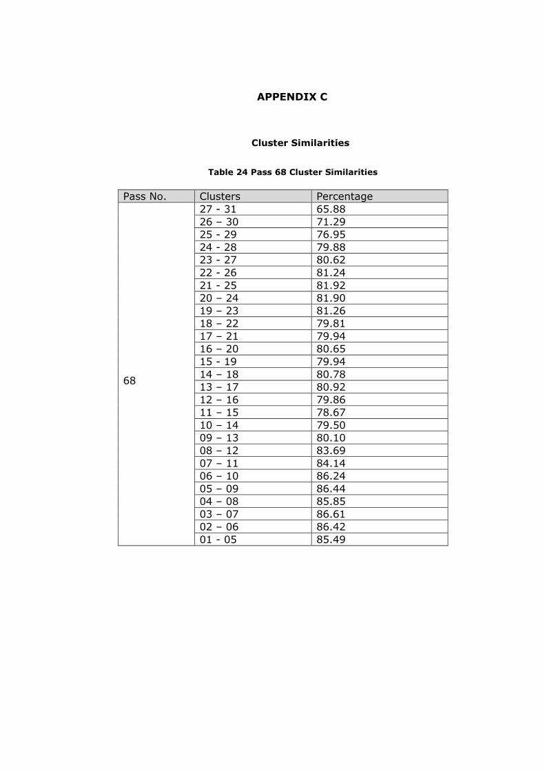
81

APPENDIX C

C: Cluster Similarities

Table 24 Pass 68 Cluster Similarities

Pass No. Clusters Percentage 68

27 - 31 65.88 26 – 30 71.29 25 - 29 76.95 24 - 28 79.88 23 - 27 80.62 22 - 26 81.24 21 - 25 81.92 20 – 24 81.90 19 – 23 81.26 18 – 22 79.81 17 – 21 79.94 16 – 20 80.65 15 - 19 79.94 14 – 18 80.78 13 – 17 80.92 12 – 16 79.86 11 – 15 78.67 10 – 14 79.50 09 – 13 80.10 08 – 12 83.69 07 – 11 84.14 06 – 10 86.24 05 – 09 86.44 04 – 08 85.85 03 – 07 86.61 02 – 06 86.42 01 - 05 85.49

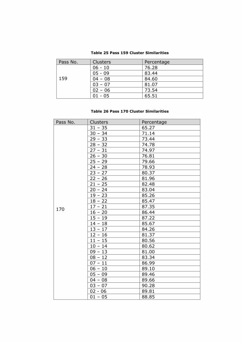
82

Table 25 Pass 159 Cluster Similarities

Pass No. Clusters Percentage 159

06 - 10 76.28 05 - 09 83.44 04 – 08 84.60 03 – 07 81.07 02 – 06 73.54 01 - 05 65.51

Table 26 Pass 170 Cluster Similarities

Pass No. Clusters Percentage 170

31 – 35 65.27 30 – 34 71.14 29 – 33 73.44 28 – 32 74.78 27 – 31 74.97 26 – 30 76.81 25 – 29 79.66 24 – 28 78.93 23 – 27 80.37 22 – 26 81.96 21 – 25 82.48 20 – 24 83.04 19 – 23 85.26 18 – 22 85.47 17 – 21 87.35 16 – 20 86.44 15 – 19 87.22 14 – 18 85.67 13 – 17 84.26 12 – 16 81.37 11 – 15 80.56 10 – 14 80.62 09 – 13 81.00 08 – 12 83.34 07 – 11 86.99 06 – 10 89.10 05 – 09 89.46 04 – 08 89.66 03 – 07 90.28 02 - 06 89.81 01 – 05 88.85

83

Pass No. Clusters Percentage 246

24 – 28 69.66 23 – 27 72.68 22 – 26 74.96 21 – 25 77.80 20 – 24 76.26 19 – 23 76.61 18 – 22 73.99 17 – 21 65.86 16 – 20 59.37 15 – 19 57.99 14 – 18 56.75 13 – 17 61.17 12 – 16 71.78 11 – 15 76.73 10 – 14 82.02 09 – 13 84.31 08 – 12 85.08 07 – 11 84.26 06 – 10 84.96 05 – 09 85.39 04 – 08 86.60 03 – 07 86.01 02 - 06 85.61 01 - 05 84.37

Table 27 Pass 246 Cluster Similarities

84

APPENDIX D

D: Cluster Trends

(Pass 68, 159, 170. 246 respectively. Unit is mm. for trends and std.)

Table 28 Cluster Trends of Pass 68

t table value 1.28 1 trend 6.1 ± 1.5 t_test 4.06 2 trend 5.7 ± 1.5 t_test 3.78 3 trend 6.6 ± 1.5 t_test 4.40 4 trend 4.5 ± 1.5 t_test 3.09 5 trend 5.2 ± 1.5 t_test 3.53 6 trend 6.2 ± 1.5 t_test 4.15 7 trend 6.3 ± 1.5 t_test 4.22 8 trend 5.9 ± 1.5 t_test 4.03 9 trend 6.3 ± 1.5 t_test 4.15 10 trend 7.7 ± 1.5 t_test 5.08 11 trend 5.5 ± 1.5 t_test 3.52 12 trend 5.9 ± 1.5 t_test 3.98 13 trend 5.1 ± 1.4 t_test 3.61 14 trend 6.5 ± 1.4 t_test 4.55 15 trend 5.3 ± 1.4 t_test 3.71 16 trend 6.3 ± 1.5 t_test 4.26 17 trend 5.9 ± 1.5 t_test 4.00 18 trend 4.1 ± 1.5 t_test 2.72 19 trend 5.3 ± 1.6 t_test 3.35 20 trend 6.3 ± 1.5 t_test 4.25 21 trend 4.2 ± 1.5 t_test 2.71 22 trend 5.6 ± 1.5 t_test 3.71 23 trend 3.4 ± 1.5 t_test 2.35 24 trend 3.9 ± 1.4 t_test 2.70 25 trend 3.7 ± 1.5 t_test 2.48 26 trend 2.9 ± 1.4 t_test 2.02 27 trend 3.1 ± 1.6 t_test 1.97 28 trend 2.6 ± 1.6 t_test 1.59 29 trend 0.1 ± 1.5 t_test 0.09 30 trend-1.0 ± 1.6 t_test 0.62 31 trend-2.0 ± 1.3 t_test 1.51

85

Table 29 Cluster Trends of Pass 159

t table value1.28 1 trend 2.3 ± 1.3 t_test 1.77 2 trend 4.4 ± 1.3 t_test 3.45 3 trend 5.3 ± 1.4 t_test 3.80 4 trend 6.8 ± 1.4 t_test 4.84 5 trend 7.2 ± 1.4 t_test 5.22 6 trend 9.2 ± 1.4 t_test 6.32 7 trend 8.8 ± 1.5 t_test 5.94 8 trend 8.1 ± 1.5 t_test 5.30 9 trend 6.0 ± 1.5 t_test 4.05 10 trend 2.4 ± 1.5 t_test 1.66

86

Table 30 Cluster Trends of Pass 170

t table value 1.28

1 trend 8.5 ± 1.3 t_test 6.76 2 trend 8.8 ± 1.3 t_test 6.94 3 trend 9.1 ± 1.2 t_test 7.25 4 trend 8.9 ± 1.3 t_test 7.08 5 trend 9.5 ± 1.3 t_test 7.30 6 trend 10.4 ± 1.3 t_test 7.88 7 trend 9.4 ± 1.3 t_test 7.05 8 trend 8.9 ± 1.3 t_test 6.60 9 trend 8.3 ± 1.3 t_test 6.14 10 trend 9.3 ± 1.3 t_test 6.94 11 trend 7.5 ± 1.3 t_test 5.58 12 trend 5.2 ± 1.3 t_test 4.10 13 trend 6.3 ± 1.4 t_test 4.65 14 trend 6.4 ± 1.4 t_test 4.57 15 trend 7.6 ± 1.4 t_test 5.44 16 trend 5.0 ± 1.4 t_test 3.53 17 trend 5.1 ± 1.4 t_test 3.66 18 trend 5.5 ± 1.4 t_test 3.90 19 trend 4.5 ± 1.4 t_test 3.17 20 trend 3.7 ± 1.4 t_test 2.61 21 trend 3.4 ± 1.4 t_test 2.42 22 trend 2.9 ± 1.4 t_test 2.09 23 trend 2.4 ± 1.4 t_test 1.70 24 trend 3.0 ± 1.5 t_test 2.08 25 trend 2.3 ± 1.5 t_test 1.54 26 trend 3.6 ± 1.5 t_test 2.40 27 trend 2.9 ± 1.5 t_test 1.92 28 trend 2.2 ± 1.6 t_test 1.40 29 trend 2.2 ± 1.5 t_test 1.51 30 trend-0.1 ± 1.5 t_test 0.10 31 trend 1.6 ± 1.5 t_test 1.04 32 trend 1.7 ± 1.6 t_test 1.12 33 trend 0.6 ± 1.6 t_test 0.40 34 trend-0.9 ± 1.6 t_test 0.55 35 trend-2.7 ± 1.6 t_test 1.70

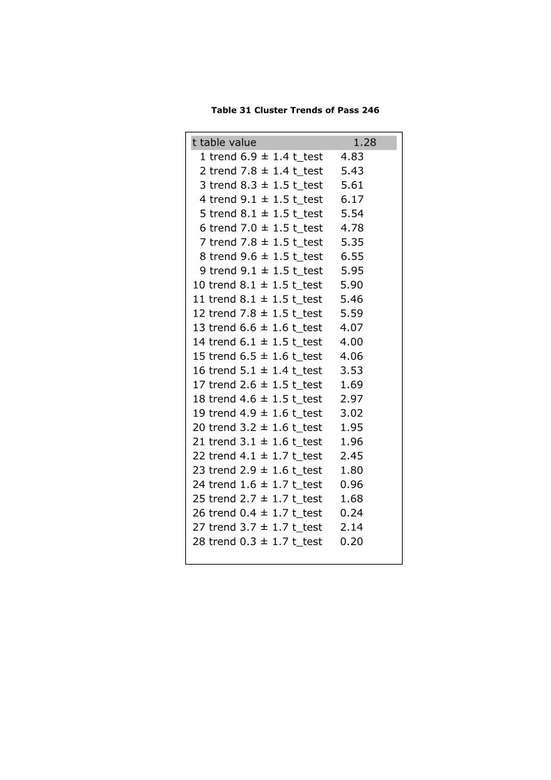
87

Table 31 Cluster Trends of Pass 246

t table value 1.28 1 trend 6.9 ± 1.4 t_test 4.83 2 trend 7.8 ± 1.4 t_test 5.43 3 trend 8.3 ± 1.5 t_test 5.61 4 trend 9.1 ± 1.5 t_test 6.17 5 trend 8.1 ± 1.5 t_test 5.54 6 trend 7.0 ± 1.5 t_test 4.78 7 trend 7.8 ± 1.5 t_test 5.35 8 trend 9.6 ± 1.5 t_test 6.55 9 trend 9.1 ± 1.5 t_test 5.95 10 trend 8.1 ± 1.5 t_test 5.90 11 trend 8.1 ± 1.5 t_test 5.46 12 trend 7.8 ± 1.5 t_test 5.59 13 trend 6.6 ± 1.6 t_test 4.07 14 trend 6.1 ± 1.5 t_test 4.00 15 trend 6.5 ± 1.6 t_test 4.06 16 trend 5.1 ± 1.4 t_test 3.53 17 trend 2.6 ± 1.5 t_test 1.69 18 trend 4.6 ± 1.5 t_test 2.97 19 trend 4.9 ± 1.6 t_test 3.02 20 trend 3.2 ± 1.6 t_test 1.95 21 trend 3.1 ± 1.6 t_test 1.96 22 trend 4.1 ± 1.7 t_test 2.45 23 trend 2.9 ± 1.6 t_test 1.80 24 trend 1.6 ± 1.7 t_test 0.96 25 trend 2.7 ± 1.7 t_test 1.68 26 trend 0.4 ± 1.7 t_test 0.24 27 trend 3.7 ± 1.7 t_test 2.14 28 trend 0.3 ± 1.7 t_test 0.20

88

APPENDIX E

E: Standard Deviations of Clusters Before and After Centered

Std. Unit is cm

Table 32 Before and After Centered Standard Dev. of Pass 68

10.27 11.08 11.20 12.02 13.07 12.92 12.22 11.37 11.39 10.91 10.70 10.54 10.30 10.15 9.57 9.94 9.59 8.60 9.26 8.53 8.63 8.56 8.41 8.94 9.28 8.99 9.95 10.98 11.29 12.81 13.20

8.59 8.59 8.60 8.24 8.39 8.58 8.61 8.43 8.66 8.62 8.79 8.59 8.14 8.29 8.41 8.47 8.38 8.59 8.94 8.48 8.66 8.57 8.16 8.29 8.47 8.04 8.87 9.48 8.79 9.60 8.54

89

Table 33 Before and After Centered Standard Dev. of Pass 159

11.16 11.07 10.85 11.42 11.71 12.42 12.19 12.50 11.92 12.51

7.88 8.12 8.33 8.17 8.10 8.62 8.65 8.91 8.52 9.17

90

Table 34 Before and After Centered Standard Dev. of Pass 170

11.76 12.49 13.44 13.32 13.05 12.58 12.14 11.74 10.76 10.04 9.49 9.14 9.70 10.52 10.77 11.33 12.20 12.62 13.34 14.86 17.08 18.64 19.47 19.96 19.81 19.06 19.19 18.96 21.07 23.78 26.42 28.24 28.32 29.39 30.84

7.47 7.55 7.47 7.46 7.71 7.93 7.93 7.95 7.92 7.97 7.98 7.40 7.86 8.02 8.11 8.07 7.95 8.05 8.01 7.97 8.04 7.97 7.98 8.23 8.54 8.58 8.73 9.24 8.52 8.65 8.68 8.95 9.26 9.23 10.46

91

Table 35 Before and After Centered Standard Dev. of Pass 246

20.44 24.08 22.07 17.43 14.93 13.50 13.01 12.19 11.23 10.44 10.24 10.17 11.02 10.85 11.68 11.34 11.87 11.58 12.96 13.41 13.57 14.20 14.84 15.41 16.55 17.39 18.14 18.06

8.23 8.60 8.39 8.40 8.41 8.47 8.57 8.59 8.73 8.78 8.77 8.78 9.35 8.88 9.45 9.20 9.73 9.28 9.40 9.42 9.09 9.49 8.99 9.55 9.80 9.73 10.26 10.03

92

APPENDIX F

F: Geodetic Coordinates (WGS84) of Cluster Centers

Table 36 Geodetic Coor. of Cluster Cent. for Pass 68

Cluster Number

Latitude Longitude

1 2 3 4 5 6 7 8 9 10 11 12 13 14 15 16 17 18 19 20 21 22 23 24 25 26 27 28 29 30 31

35.0341 35.0842 35.1333 35.1817 35.2294 35.2777 35.3257 35.3731 35.4203 35.4676 35.5148 35.5604 35.6053 35.6499 35.6946 35.7466 35.7933 35.8388 35.8836 35.9307 35.9781 36.0270 36.0766 36.1253 36.1754 36.2239 36.2709 36.3179 36.3644 36.4090 36.4493

35.3087 35.2787 35.2490 35.2196 35.1908 35.1615 35.1323 35.1035 35.0746 35.0457 35.0167 34.9888 34.9615 34.9339 34.9067 34.8744 34.8454 34.8173 34.7896 34.7603 34.7308 34.7004 34.6695 34.6392 34.6078 34.5773 34.5479 34.5186 34.4893 34.4613 34.4357

93

Table 37 Geodetic Coor. of Cluster Cent. for Pass 159

Cluster Number

Latitude Longitude

1 2 3 4 5 6 7 8 9 10

35.0200 35.0540 35.0904 35.1336 35.1800 35.2272 35.2754 35.3232 35.3704 35.4157

35.5517 35.5721 35.5942 35.6202 35.6484 35.6770 35.7062 35.7354 35.7639 35.7917

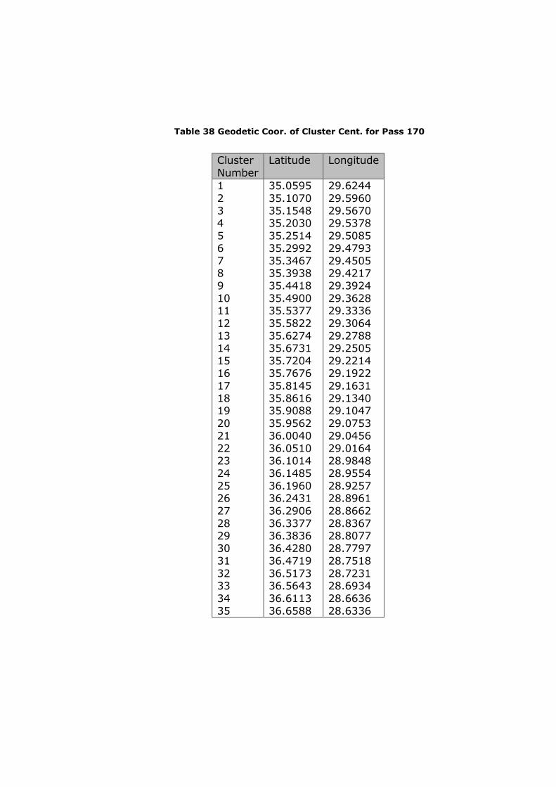
94

Cluster Number

Latitude Longitude

1 2 3 4 5 6 7 8 9 10 11 12 13 14 15 16 17 18 19 20 21 22 23 24 25 26 27 28 29 30 31 32 33 34 35

35.0595 35.1070 35.1548 35.2030 35.2514 35.2992 35.3467 35.3938 35.4418 35.4900 35.5377 35.5822 35.6274 35.6731 35.7204 35.7676 35.8145 35.8616 35.9088 35.9562 36.0040 36.0510 36.1014 36.1485 36.1960 36.2431 36.2906 36.3377 36.3836 36.4280 36.4719 36.5173 36.5643 36.6113 36.6588

29.6244 29.5960 29.5670 29.5378 29.5085 29.4793 29.4505 29.4217 29.3924 29.3628 29.3336 29.3064 29.2788 29.2505 29.2214 29.1922 29.1631 29.1340 29.1047 29.0753 29.0456 29.0164 28.9848 28.9554 28.9257 28.8961 28.8662 28.8367 28.8077 28.7797 28.7518 28.7231 28.6934 28.6636 28.6336

Table 38 Geodetic Coor. of Cluster Cent. for Pass 170

95

Cluster Number

Latitude Longitude

1 2 3 4 5 6 7 8 9 10 11 12 13 14 15 16 17 18 19 20 21 22 23 24 25 26 27 28

35.2547 35.3165 35.3792 35.4377 35.4895 35.5382 35.5855 35.6325 35.6793 35.7262 35.7723 35.8183 35.8650 35.9107 35.9549 35.9940 36.0247 36.0607 36.1053 36.1516 36.1981 36.2454 36.2929 36.3402 36.3876 36.4347 36.4804 36.5248

32.3411 32.3036 32.2650 32.2294 32.1978 32.1680 32.1390 32.1101 32.0812 32.0523 32.0238 31.9953 31.9665 31.9382 31.9105 31.8865 31.8672 31.8449 31.8169 31.7881 31.7589 31.7293 31.6993 31.6697 31.6398 31.6102 31.5815 31.5530

Table 39 Geodetic Coor. of Cluster Cent. for Pass 246

96

APPENDIX G

G: Significant Periods of Each Cluster

Table 40 Significant Periods of Pass 68

1.00438356164384 1.00438356164384 1.00438356164384 1.29597878921785, 1.00438356164384 1.00438356164384 1.00438356164384 1.00150567123288 1.00438356164384 1.00438356164384 1.00150567123288 1.00438356164384 1.03013698630137 6.69589041095890. 1.00438356164384 1.03013698630137 1.03013698630137 1.00438356164384 1.00438356164384 5, 72288954990215, 1.00150567123288 6.69589041095890.1.00438356164384 5, 73933463796478, 1.00438356164384 5, 73933463796478, 1.00438356164384 1.03013698630137 6.67670447488584, 1.00150567123288 1.02718530382859 1.02423362135581 6.61914666666667, 0.992872000000000 6.63833260273973, 0.995749890410959 6.63833260273973, 0.995749890410959 6.65751853881279, 0.998627780821917 7, 98902224657534, 0.998627780821917 6.54240292237443, 1.00652352651914

1 2 3 4 5 6 7 8 9 10 11 12 13 14 15 16 17 18 19 20 21 22 23 24 25 26 27 28 29 30 31

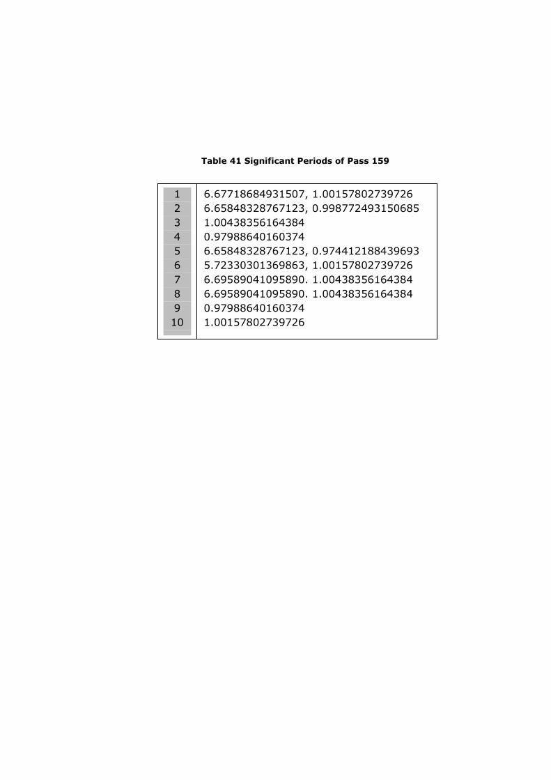
97

Table 41 Significant Periods of Pass 159

6.67718684931507, 1.00157802739726 6.65848328767123, 0.998772493150685 1.00438356164384 0.97988640160374 6.65848328767123, 0.974412188439693 5.72330301369863, 1.00157802739726 6.69589041095890. 1.00438356164384 6.69589041095890. 1.00438356164384 0.97988640160374 1.00157802739726

1 2 3 4 5 6 7 8 9 10

98

Table 42 Significant Periods of Pass 170

1.00157802739726 1.00438356164384 1.00438356164384 1.00438356164384 1.00438356164384 1.00438356164384 1.00438356164384 1.03013698630137 1.03013698630137 1.00438356164384 1.00438356164384 1.00438356164384 1.00438356164384 1.00438356164384 1.03013698630137 1.00438356164384 1.03013698630137 1.02725951527924 1.02725951527924 1.02725951527924 6.67718684931507, 1.00157802739726 6.67718684931507, 1.00157802739726 6.69589041095890. 1.00438356164384 6.69589041095890. 1.00438356164384 6.69589041095890. 1.00438356164384 6.67718684931507, 1.00157802739726 6.67718684931507, 1.00157802739726 6.69589041095890. 1.00438356164384 6.69589041095890. 1.00438356164384 6.69589041095890. 1.00438356164384 6.69589041095890. 1.00438356164384 6.69589041095890. 1.00438356164384 8.03506849315069, 1.00438356164384 6.65848328767123, 0.974412188439693 6.65848328767123, 0.998772493150685

1 2 3 4 5 6 7 8 9 10 11 12 13 14 15 16 17 18 19 20 21 22 23 24 25 26 27 28 29 30 31 32 33 34 35

99

Table 43 Significant Periods of Pass 246

0.979886401603742 1.00438356164384 1.00438356164384 1.03013698630137 1.03013698630137 0.977118369528901 0.979886401603742 0.979886401603742 0.979886401603742 2.11449170872386, 1.03013698630137 1.03013698630137 2.11449170872386, 1.03013698630137 0.977118369528901 1.03013698630137 0.979886401603742 0.974350310725025 1.00438356164384 0.977118369528901 1.03013698630137 6.69589041095890, 1.03013698630137 6.69589041095890, 0.979886401603742 6.69589041095890, 0.979886401603742 0.979886401603742 6.69589041095890, 1.00438356164384 6.69589041095890.1.00438356164384, 0.9798864016037 8,01237063013699,1.00154632876712 6.69589041095890, 1.00438356164384 7.98967254794521, 0.998709068493150

1 2 3 4 5 6 7 8 9 10 11 12 13 14 15 16 17 18 19 20 21 22 23 24 25 26 27 28

100

APPENDIX H

H: Leading Three Spatial Models of Variability of Chosen Clusters

(68, 159, 170, and 246 respectively)

Figure 21 Leading Spatial Models for Pass 68

101

Figure 22 Leading Spatial Models for Pass 159

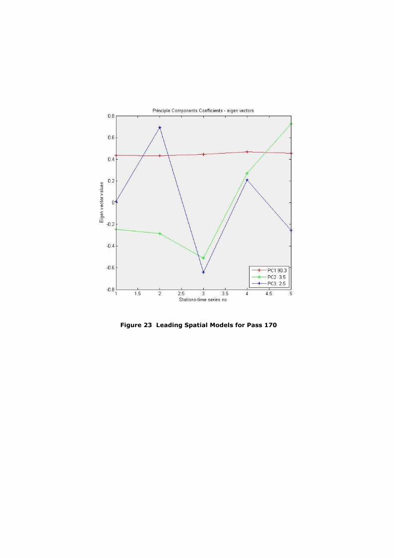
102

Figure 23 Leading Spatial Models for Pass 170

103

Figure 24 Leading Spatial Models for Pass 246