determining groundwater sources and ages via …
TRANSCRIPT

Montana Tech LibraryDigital Commons @ Montana Tech
Graduate Theses & Non-Theses Student Scholarship
Summer 2016
DETERMINING GROUNDWATERSOURCES AND AGES VIA ISOTOPEGEOCHEMISTRY IN BIG SKY, MONTANAThomson ConnieMontana Tech of the University of Montana
Follow this and additional works at: http://digitalcommons.mtech.edu/grad_rsch
Part of the Geology Commons
This Thesis is brought to you for free and open access by the Student Scholarship at Digital Commons @ Montana Tech. It has been accepted forinclusion in Graduate Theses & Non-Theses by an authorized administrator of Digital Commons @ Montana Tech. For more information, pleasecontact [email protected].
Recommended CitationConnie, Thomson, "DETERMINING GROUNDWATER SOURCES AND AGES VIA ISOTOPE GEOCHEMISTRY IN BIG SKY,MONTANA" (2016). Graduate Theses & Non-Theses. 94.http://digitalcommons.mtech.edu/grad_rsch/94

DETERMINING GROUNDWATER SOURCES AND AGES VIA ISOTOPE
GEOCHEMISTRY IN BIG SKY, MONTANA
by
Connie J. Thomson
A thesis submitted in partial fulfillment of the
requirements for the degree of
Master of Science in Geoscience:
Hydrogeological Engineering Option
Montana Tech
2016

ii
Abstract
The Big Sky ski resort area in southwestern Montana is experiencing exponential growth in both
development and population. Concerns have arisen over the quantity of good-quality
groundwater in the region, and whether there is a large enough reserve to support the growing
demand. In light of already-documented water-level decreases, and domestic wells needing to be
deepened or replaced, the Montana Department of Natural Resources and Conservation (DNRC)
enlisted the Montana Bureau of Mines and Geology's Ground Water Investigation Program to
perform an assessment of groundwater availability and quality in the region, and define
groundwater supply sources.
The geology in the region is complex. Faulting and folding have disturbed the once horizontal
rock layers. Sub-surface rock layers that act as good aquifers (sources of groundwater) in one
part of the greater Big Sky area can be dry or have poor quality water just a few miles away. This
complexity adds to the challenge of performing a groundwater survey.
Several water chemistry parameters were studied in hopes of answering the groundwater
questions in Big Sky. Samples were collected from groundwater and surface water sites across
the study area for water isotopes (oxygen-18 and deuterium), carbon isotopes, tritium, and full
dissolved mineral analyses. The hope was to find a distinct chemical signature for each aquifer
and/or sub-region of the study area. Surface water-groundwater interactions were also examined.
The isotopic results alone were not enough to fingerprint waters in the study area, but combined
with water chemistry they did. There was an abundance of evidence of mixing, both vertically
between aquifers (especially between the Kootenai and Morrison Formations) and horizontally
(within regional areas). The alluvial aquifer in the Meadow Village area was found to be almost
completely disconnected from the underlying bedrock. Interaction between groundwater and
surface water was evident in both the Meadow Village area, and in Yellowstone Club and
Spanish Peaks, along the South Fork of the West Fork Gallatin River. An overall trend of gaining
streams was revealed, which is a good indication that the groundwater supply is currently
sufficient for the area’s needs.
Keywords: hydrogeology, geochemistry, water isotopes, carbon isotopes, groundwater, tritium

iii
Dedication
This thesis is dedicated to the memory of my high school science teacher, Les Wagner. I never
would have taken this path without his guidance, influence, and encouragement. He was a
brilliant man who could have done scientific research anywhere, in a dozen different
disciplines…and he chose to teach high school science in a tiny North Dakota town. We were the
luckiest students in the world.
You are greatly missed, Mr. Wagner.

iv
Acknowledgements
My thesis research was made possible by the Ground Water Investigation Program of the
Montana Bureau of Mines and Geology. My deepest gratitude is extended to everyone there,
especially Program Manager Ginette Abdo and my immediate supervisors, James Rose and Kirk
Waren. Great thanks to my academic/thesis advisor, Dr. Glenn Shaw, and the rest of my thesis
committee - Dr. Chris Gammons, Dr. Alysia Cox, and James Rose. To all my instructors in the
geological engineering, general engineering, and chemistry/geochemistry departments, for the
top-notch education I have received at Montana Tech. All of my water isotope and water quality
samples were processed by Jackie Timmer and Ashley Huft in the MBMG Analytical
Laboratory; thank you so much. Thank you to Dr. Stephen Parker for running my carbon
samples and for being a great sounding board. Thank you to Dr. Simon Poulson at the University
of Reno for analyzing my sulfur isotope samples. Finally, fellow MBMG employees Allison
Brown, Matt Berzel, and Dean Snyder helped us in the field – we could not have collected all
those samples and monitored all those wells without you!

v
Table of Contents
ABSTRACT ................................................................................................................................................ II
DEDICATION ........................................................................................................................................... III
ACKNOWLEDGEMENTS ........................................................................................................................... IV
LIST OF TABLES ..................................................................................................................................... VIII
LIST OF FIGURES ....................................................................................................................................... X
LIST OF EQUATIONS .............................................................................................................................. XIII
1. INTRODUCTION ................................................................................................................................. 1
1.1. Isotopes in Water ............................................................................................................... 3
1.1.1. Notations for Stable Isotopes .............................................................................................................. 5
1.1.2. Isotopes Selected ................................................................................................................................ 6
1.2. Water Chemistry and Quality ........................................................................................... 10
1.3. Previous Work .................................................................................................................. 14
2. STUDY AREA ................................................................................................................................... 17
2.1. Location, History, and Demographics .............................................................................. 17
2.2. Geography and Topography ............................................................................................ 18
2.3. Climate ............................................................................................................................. 19
2.4. Surface Water .................................................................................................................. 21
2.5. Geology ............................................................................................................................ 22
2.5.1. Individual Geologic Units ................................................................................................................... 24
2.5.2. Structural Geology and Landslides .................................................................................................... 27
3. METHODS ...................................................................................................................................... 28
3.1. Field Methods and Materials ........................................................................................... 28
3.2. Analytical Methods .......................................................................................................... 33
vi
3.2.1. Sulfur/Sulfate Samples ...................................................................................................................... 35
3.2.2. Tritium Samples ................................................................................................................................. 36
4. RESULTS ......................................................................................................................................... 37
4.1. Laboratory Results ........................................................................................................... 37
4.1.1. Oxygen-18 and Deuterium ................................................................................................................ 37
4.1.2. DIC, DOC, and Carbon-13 .................................................................................................................. 41
4.1.3. Sulfur Isotopes ................................................................................................................................... 43
4.1.4. Tritium Samples ................................................................................................................................. 44
4.1.5. Water Quality .................................................................................................................................... 45
4.1.6. Water Types ...................................................................................................................................... 48
4.2. Field Analysis Results........................................................................................................ 53
5. ANALYSIS AND DISCUSSION ................................................................................................................ 56
5.1. Analysis by Aquifer ........................................................................................................... 60
5.1.1. Alluvium/Sand and Gravel ................................................................................................................. 66
5.1.2. Rock Glacier ....................................................................................................................................... 70
5.1.3. Dacite Sills ......................................................................................................................................... 71
5.1.4. Frontier Formation ............................................................................................................................ 74
5.1.5. Mowry Shale...................................................................................................................................... 75
5.1.6. Muddy Sandstone ............................................................................................................................. 78
5.1.7. Kootenai Formation ........................................................................................................................... 84
5.1.8. Morrison Formation .......................................................................................................................... 87
5.1.9. Madison Group .................................................................................................................................. 91
5.1.10. Summary of Findings by Aquifer/Geologic Unit .............................................................................. 92
5.2. Analysis by Region ............................................................................................................ 95
5.2.1. Moonlight Basin .............................................................................................................................. 101
5.2.2. Mountain Village ............................................................................................................................. 105
5.2.3. Meadow Village ............................................................................................................................... 107
5.2.4. Spanish Peaks .................................................................................................................................. 110
5.2.5. Yellowstone Club ............................................................................................................................. 112
vii
5.2.6. Summary of Findings by Region ...................................................................................................... 114
5.3. Connections and Mixing between Aquifers and Regions ............................................... 116
5.4. Uncertainty .................................................................................................................... 122
6. CONCLUSIONS AND RECOMMENDATIONS FOR FUTURE WORK ................................................................ 124
6.1. Conclusions ..................................................................................................................... 124
6.2. Recommendations for Future Work ............................................................................... 125
7. REFERENCES CITED ......................................................................................................................... 128
8. APPENDIX A: TOPOGRAPHIC MAP OF STUDY AREA (MAP SCALE IN METERS, STUDY AREA OUTLINE IN PURPLE, GROUNDWATER
SITES LABELED BY GWIC ID) ......................................................................................................................... 132
9. APPENDIX B: SITE LOCATION INFORMATION........................................................................................ 133
10. APPENDIX C: FIELD AND WATER ISOTOPE (18O AND D) DATA ................................................................ 136
11. APPENDIX D: RAW WATER CHEMISTRY DATA, MAJOR CATIONS ............................................................. 141
12. APPENDIX E: RAW WATER CHEMISTRY DATA, MAJOR ANIONS ............................................................... 143
13. APPENDIX F: RAW WATER CHEMISTRY DATA, SELECT CONSTITUENTS ...................................................... 145
14. APPENDIX G: STIFF DIAGRAMS FOR EACH WATER QUALITY SAMPLE ........................................................ 147

viii
List of Tables
Table I: Stable Isotope Ratios for Standards........................................................................5
Table II: EPA and NRCS Water Quality Standards ..........................................................11
Table III: Isotope Sample Site Type Totals .......................................................................29
Table IV: Summary of Water Analyses .............................................................................30
Table V: Differences in Lab Results for Two Isotope Samples ........................................40
Table VI: Summary of Carbon Suite Results, plus pH Values ..........................................41
Table VII: Sulfur Isotope Results ......................................................................................43
Table VIII: Tritium Results ...............................................................................................44
Table IX: Summary of Water Quality Exceedances ..........................................................46
Table X: Summary of Water Types ...................................................................................49
Table XI: Field Alkalinity Concentrations ........................................................................55
Table XII: Field Sulfide Concentrations ............................................................................55
Table XIII: Water Isotope Values by Geologic Unit .........................................................61
Table XIV: pH and Carbon Data by Unit ..........................................................................63
Table XV: Average pH and Carbon Values by Unit .........................................................63
Table XVI: Tritium Concentrations by Unit ......................................................................66
Table XVII: Water Types in the Alluvium Aquifer ...........................................................69
Table XVIII: Water Types in Dacite Sills .........................................................................74
Table XIX: Water Types in Mowry Aquifer .....................................................................77
Table XX: Water Types in Muddy Aquifer .......................................................................83
Table XXI: Water Types in Kootenai Aquifer ..................................................................87
Table XXII: Water Types in Morrison Aquifer .................................................................90
ix
Table XXIII: Water Isotope Values by Region .................................................................95
Table XXIV: Carbon Results Sorted by Region ................................................................98
Table XXV: Carbon Averages and Standard Deviations, by Region ................................98
Table XXVI: Tritium Concentrations, by Region ...........................................................101
Table XXVII: Water Types in Moonlight Basin .............................................................104
Table XXVIII: Water Types in Mountain Village ...........................................................107
Table XXIX: Water Types in Meadow Village ...............................................................109
Table XXX: Water Types in Spanish Peaks ....................................................................111
Table XXXI: Water Types in Yellowstone Club .............................................................114
Table XXXII: Water Isotope Averages and Standard Deviations, by Water Type .........118

x
List of Figures
Figure 1: Identifying DOC Sources by C/N Ratio vs. δ13C Concentration (Eby, 2004) .....8
Figure 2: Geographical Location of Study Area. (Images on left, NAIP GIS. Image on right,
Google Earth.) ........................................................................................................17
Figure 3: Regions and Major Mountain Peaks of Study Area. (Image: Google Earth) .....19
Figure 4: West Fork of the Gallatin River and its Forks and Tributaries in Big Sky ........21
Figure 5: Surface Geology of Big Sky (modified from Kellogg and Williams, 2006). Lines A-A’
and B-B’ represent cross sections shown in Figure 6. Thick black solid line represents the
Spanish Peaks Fault; thick black dashed line represents Hilgard thrust system. Thinner
black lines are folds and lesser faults. Thin black dotted line is the MBMG GWCP study
area. Blue and yellow circles are wells used in the GWCP study. Geologic units are
symbolized by: Qal and Qgr = alluvium, Qls = landslide deposit, Qgt = glacial till, Qrg=
rock glacier, Qc = colluvium, TKga = gabbro intrusion, Thr =welded tuff extrusion, Kdap
= dacite intrusion, Kco = Cody shale, Kf = Frontier Formation, Km = Mowry Shale,
Kmdt = Muddy Sandstone, Kk = Kootenai Formation, JTmd = Morrison through
Dinwoody Formations, Psh = Shedhorn Sandstone, IPMqa = Quadrant and Amsden
Formations, Mm = Madison limestone. .................................................................23
Figure 6: Geologic Cross Sections from Figure 5 (modified from Vuke, 2013). ..............24
Figure 7: All Isotope Sample Sites in Big Sky Study Area ...............................................28
Figure 8: Sites of Water Quality and Carbon Suite Samples .............................................30
Figure 9: Sites of Tritium, Field Sulfide, and Sulfur Isotope Samples (All Groundwater)31
Figure 10: Plot of Preliminary Big Sky Local Meteoric Water Line (LMWL) .................38
Figure 11: All Big Sky Isotope Results .............................................................................39

xi
Figure 12: Piper Diagram for Groundwater Samples. Legend translation: 111SNGR =
Alluvium/Sand and Gravel, 112RKGL = Rock Glacier, 211FRNR = Frontier Formation,
211PLNC = Dacite Sills, 217KOTN = Kootenai Formation, 217MDDY = Muddy
Sandstone, 217MWRY = Mowry Shale, 221MRSN = Morrison Formation, 330MDSN =
Madison Limestone Group. ...................................................................................51
Figure 13: Piper Diagram for Surface Water, Precipitation, and Effluent Samples ..........52
Figure 14: Stiff Diagram for an Alluvial Well, Presented as a Representative Example ..53
Figure 15: Detailed map for Meadow Village Area. Topographic scale in feet. ...............57
Figure 16: Detailed map for Moonlight Basin and Mountain Village. Topographic scale in feet.
................................................................................................................................58
Figure 17: Detailed map for Yellowstone Club and Spanish Peaks. Topographic scale in feet.
................................................................................................................................59
Figure 18: Groundwater Isotopes, by Geologic Unit .........................................................60
Figure 19: Average Water Isotope Values by Unit and Precipitation Source, with Standard
Deviation ................................................................................................................61
Figure 20: Average Water Isotope Values by Unit, with Standard Deviation...................62
Figure 21: Carbon-13 vs. DIC Concentration, by Aquifer ................................................64
Figure 22: Carbon-13 vs. 1/DIC, by Aquifer .....................................................................64
Figure 23: Carbon-13 vs. DOC Concentration, by Aquifer ...............................................65
Figure 24: Carbon-13 vs. 1/DOC, by Aquifer ...................................................................65
Figure 25: Water Isotopes in Alluvium Aquifer ................................................................67
Figure 26: Water Isotopes in Dacite Sills ..........................................................................72
Figure 27: Water Isotopes in Mowry Aquifer....................................................................77

xii
Figure 28: Water Isotopes in Muddy Aquifer ....................................................................80
Figure 29: Water Isotopes in Kootenai Aquifer .................................................................85
Figure 30: Water Isotopes in Morrison Aquifer ................................................................88
Figure 31: Water Isotopes by Region ................................................................................95
Figure 32: Water Isotopes Averages by Region and Precipitation Source, plus Standard
Deviation ................................................................................................................96
Figure 33: Water Isotope Averages by Region, plus Standard Deviation .........................97
Figure 34: Carbon-13 vs. DIC, by Region .........................................................................99
Figure 35: Carbon-13 vs. 1/DIC, by Region ......................................................................99
Figure 36: Carbon-13 vs. DOC, by Region .....................................................................100
Figure 37: Carbon-13 vs. 1/DOC, by Region ..................................................................100
Figure 38: Water Isotope Values in Moonlight Basin .....................................................102
Figure 39: Water Isotope Values in Mountain Village ....................................................105
Figure 40: Water Isotope Values in Meadow Village. The isolated data point belongs to well
104510..................................................................................................................108
Figure 41: Water Isotope Values in Spanish Peaks .........................................................110
Figure 42: Water Isotope Values in Yellowstone Club ...................................................112
Figure 43: Piper Diagrams for Groundwater and Surface Water, with Hydrofacies .......117
Figure 44: δ13C vs. 1/DIC, by aquifer, with possible mixing lines in dashed black. .......118
Figure 45: δ13C vs. 1/DIC, by region, with possible mixing lines in dashed black. ........120
Figure 46: Deuterium vs. SC. Triangles represent possible mixing. ...............................121

xiii
List of Equations
Equation (1): Delta Notation for Stable Isotopes .................................................................5
Equation (2): Delta Notation for Oxygen-18 .......................................................................5
Equation (3): Tritium Unit Calculation................................................................................9
Equation (4): Sodium Adsorption Ratio Calculation .........................................................13
Equation (5): Global Meteoric Water Line (GMWL) ........................................................37
Equation (6): Butte Local Meteoric Water Line (LMWL) ................................................37
Equation (7): Preliminary Big Sky LMWL .......................................................................37

1
1. Introduction
Water is essential to life, second only to a breathable atmosphere for land-based plants
and creatures. Humans, animals, and the crops used as food for both, all rely on an adequate
supply of water, at different levels of purity appropriate for each organism. While a number of
life forms can survive and even thrive in or using water that would be harmful to other plants and
animals, the US Environmental Protection Agency (EPA) and US Department of Agriculture’s
Natural Resources Conservation Service (NRCS) have determined safety standards for drinking
water, livestock, irrigation, and aquatic life for a large number of major ions, trace metals,
contaminants, and more.
Whenever a new real estate development is proposed – for housing, businesses,
cultivation, or livestock grazing – one of the first questions to be answered should always be
whether there is enough water available to support the increase in usage. To answer that
question, other queries are raised: what will the primary sources of water be – surface sources or
groundwater? Are those sources large enough to maintain expected water usage under typical
recharge conditions? Is the water of potable quality; could it be used in other ways if it is not
drinkable? Are there already useable wells in place; if not, can they be drilled? If the answer to
any of these questions is no, is piping or transporting water in an affordable option? Often, it is
not, so the availability of a good-quality, sustainable water source on-site is a deal-breaker for
nearly any expansion of land use.
These are the questions being raised in Big Sky, Montana, a ski resort that continues to
expand in both physical land area and in population. A five-well system, maintained by the Big
Sky Water and Sewer District (BSWSD), currently provides the public water supply (PWS) and
sewer system for most of the businesses and residences in the Meadow Village area. Other PWS

2
wells throughout the resort development supply water to other businesses and housing centers.
Private wells supply businesses and residences outside of the BSWSD domain.
These wells are completed in a number of different aquifers, mostly various layers of
bedrock. The geology of the area is very complex; not only do multiple units act as aquifers, but
those units are discontinuous, broken by faults and folds. A geologic unit that serves as an
excellent aquifer in one location may have poor quality or insufficient water just a mile away, or
that unit may not be present at all.
Newly acquired acreage, numerous construction plans for housing, businesses, and
recreation areas, and increasing permanent and tourist populations will all tax the existing water
supply. Some land owners have already had to deepen existing wells or drill new ones entirely
due to water-level declines. These water right applications for new wells to the Montana
Department of Natural Resources and Conservation (DNRC) were one of the driving factors in
the involvement of the Ground Water Investigation Program (GWIP) of the Montana Bureau of
Mines and Geology (MBMG) in a groundwater availability study in the Big Sky region.
As GWIP works to answer the questions at hand, one of the analyses that may help is the
use of isotope geochemistry. The purpose of this study is to determine any similarities within
water sources and connections between water sources (groundwater flowpaths, recharge and
discharge areas) by analyzing their concentrations of various isotopes. Those patterns and
connections will be compared to the conclusions of previous studies. Water chemistry will also
be analyzed in conjunction with the isotopes. The main objective is to determine distinct
chemical and isotopic signatures for various water sources, by aquifer or by geographic location.
Sample results will be examined on a spatial scale in search of indications of flowpaths or
regions of mixing water sources. Finally, time since water recharge will be determined where

3
possible through analysis of tritium isotopes and water chemistry parameters. The conclusions
drawn from these analyses will assist in locating productive, high-quality water sources, and for
development planning.
1.1. Isotopes in Water
Isotopes are variant atoms of an element containing the same number of protons, but a
different number of neutrons, in their nuclei. An element is defined by the number of positively
charged protons in its atomic nucleus; in its normal state, each atom will have a matching
number of negatively charged electrons to balance the atom’s charge to zero. Neutrons are
uncharged particles and do not affect the atom’s charge, but do affect the atom’s mass. Isotopes
are notated by their atomic mass number, which is the total number of protons and neutrons in
the nucleus. As an example, the most abundant isotope of oxygen is oxygen-16, which has eight
protons and eight neutrons. It is identified by the symbol O816
. The superscript is the atomic mass
number, and the subscript is the atomic number (the number of protons in the nucleus). The
symbol for the second most common of oxygen’s isotopes, oxygen-18, is identified by the
symbol O818
, indicating that while the atom still has eight protons, it has a total of eighteen
protons and neutrons (i.e., two additional neutrons compared to oxygen-16). The atomic number
is often omitted from these symbols (18O, for example); this convention will be followed from
this point forward.
Some isotopes are stable, while others are radioactive. Stable isotopes will not break
down or decay, while radioactive isotopes will spontaneously undergo radioactive decay, and the
decaying nuclei will form other isotopes. Both types of isotopes have a number of scientific
applications. In terms of water studies, stable isotopes are used to make connections about the
source of water, and determine what processes may have occurred within that water (for

4
example, after it entered an aquifer). They act as natural markers or tracers in groundwater; their
concentrations can be used to connect waters back to their source or origin (Gat, 1996; Kendall
and Caldwell, 1998; Clark, 2015), give indication of a correlation or mixing of two waters
(Kendall and Caldwell, 1998; Genereux et al., 2009), or show flowpaths in a region (Kendall and
Caldwell, 1998; Singleton and Moran, 2010). Radioactive isotopes are generally used for age
dating of waters (Eby, 2004).
Most elements have known isotopes, and for the most part, the different isotopes of an
element remain nearly identical in terms of chemical behavior, as they still have the same
number of protons. However, there are some small variances that occur due to the differences in
mass between isotopes. In the heavier elements – Eby (2004) suggests all elements with an
atomic mass of 40 and higher – the addition or subtraction of just a few neutrons makes little
difference in terms of stable isotopes. In the lighter elements, though, the relative mass
difference between isotopes is a much larger portion of the total mass of an atom of that element.
These differences in mass cause isotopic fractionation: any physical, chemical, or biological
process that causes the isotopic ratios to vary from one region or phase to another (Eby, 2004;
Drever, 1997; Fetter, 2001). Isotopic concentrations can also be influenced by outside sources,
such as nuclear reactions.
It should also be noted that while many isotopes are naturally occurring, others can only
be produced in a laboratory setting. Also, isotopes can be lighter than the most abundant isotope
(containing fewer neutrons) but they occur less frequently than heavier isotopes, and are often
both lab-created and unstable.

5
1.1.1. Notations for Stable Isotopes
Most stable isotope concentrations are expressed using delta notation (δ). Since the
isotopes in question occur in very small amounts (they usually have abundances of less than 1%),
it is not feasible to report absolute isotopic ratios. The delta notation is a representation of the
relative difference between the ratio of isotopes in a sample and the ratio in a standard specific to
those isotopes. The general equation is:
𝛿𝑠𝑎𝑚𝑝𝑙𝑒 (‰) = (𝑅𝑠𝑎𝑚𝑝𝑙𝑒 − 𝑅𝑠𝑡𝑎𝑛𝑑𝑎𝑟𝑑
𝑅𝑠𝑡𝑎𝑛𝑑𝑎𝑟𝑑) × 1000 = (
𝑅𝑠𝑎𝑚𝑝𝑙𝑒
𝑅𝑠𝑡𝑎𝑛𝑑𝑎𝑟𝑑− 1) × 1000 (1)
where Rsample is the isotopic ratio in question present in the sample (less abundant isotope to most
abundant isotope, by convention), and Rstandard is the isotopic ratio present in a standard (Fetter,
2001). For example, δ18O is expressed as:
𝛿 O18 (‰) =
(
O18
O16𝑠𝑎𝑚𝑝𝑙𝑒
O18
O16𝑠𝑡𝑎𝑛𝑑𝑎𝑟𝑑
− 1
)
× 1000 (2)
The unit for delta notation is per mil (‰), or parts per thousand. Deuterium, carbon-13,
and sulfur-34 concentrations are represented by δD (or δ2H), δ13C, and δ34S, respectively. The
use of consistent standards is the key for ensuring accurate comparisons of test results. The
standards used for δ18O, δD, δ13C, and δ34S are listed in Table I (Eby, 2004).
Table I: Stable Isotope Ratios for Standards
Element Standard Ratio
Oxygen Vienna Standard Mean Ocean Water (VSMOW) 18O/16O = 2005.20∙(10-6)
Hydrogen Vienna Standard Mean Ocean Water (VSMOW) 2H/1H = 155.76∙(10-6)
Carbon Vienna Pee Dee Belemnite (VPDB) 13C/12C = 1123.72∙(10-5)
Sulfur Canyon Diablo Troilite (CDT) 34S/32S = 449.94∙(10-4)
If the delta value for a water sample is positive, that means it is enriched in the heavier
isotope (oxygen-18, for example) relative to the standard. If the delta value is negative, the

6
sample is depleted with respect to that isotope, relative to the standard. When comparing two
negative delta values, the less negative (closer to zero) value is considered the more enriched of
the two; likewise, the more negative value is considered the more depleted.
1.1.2. Isotopes Selected
The isotopes oxygen-18 ( O18 ) and hydrogen-2 (deuterium, symbolized by 2H or D) are
the most studied water isotopes, and their characteristics were determined to be applicable for
this project. Both oxygen-18 and deuterium are heavy isotopes of their respective elements;
oxygen-18 has two additional neutrons compared to most abundant oxygen-16, and deuterium
has one neutron, where hydrogen-1 has none. Oxygen-18 has an average terrestrial abundance of
0.2%, and deuterium of 0.015% (Eby, 2004)
Water molecules containing even just one heavy isotopic atom will have greater mass
than a standard water molecule. These heavy water molecules require more energy to move from
the liquid to vapor phase than standard water molecules; as a body of water evaporates, the water
left behind will become increasingly enriched with respect to the heavier isotopes (Eby, 2004).
Unevaporated waters that are relatively enriched in oxygen-18 and deuterium usually originate
from precipitation in the form of rain, falling at lower elevations. Those that are relatively
depleted with respect to oxygen-18 and deuterium are most often from snowfall at relatively
higher elevations (Clark, 2015). As a result, the isotopic concentration of the water that remains
can act as a fingerprinting tool or a natural tracer, indicating where the water came from, where it
has been, and what interactions it has had (Kendall and Caldwell, 1998). Further, isotope
concentrations in groundwater that are close to the concentrations in rainfall can help identify
recharge sites near the surface (Gat, 1996). Isotope concentrations in deeper, bedrock

7
groundwater are generally conservative, not changing unless elevated temperatures (greater than
150°C) cause chemical interaction with the country rock (Gat, 1996).
In this study, the isotope carbon-13 was also analyzed. It has one additional neutron over
the more common carbon-12, and occurs at an abundance of about 1.1% (Eby, 2004). Carbon-13
concentrations can indicate sources of both dissolved inorganic and dissolved organic carbon in
groundwater (Clark and Fritz, 1997; Fetter, 2001; Eby, 2004). Most of the dissolved inorganic
carbon (DIC) in groundwater comes from soil-zone carbon dioxide gas (generated by soil biota)
and dissolution of carbonate rocks. Atmospheric carbon dioxide has a δ13C value around -7‰
(Eby, 2004), but is generally a very small contributor to carbon in groundwater because of its
low partial pressure (Fetter, 2001). Soil-zone CO2 is typically strongly depleted in carbon-13
(δ13C = -20 to -30‰) due to isotopic fractionation by microorganisms that degrade organic
carbon. Marine limestones have δ13C near 0‰, so dissolution of calcite in marine limestone or
dolomite will yield δ13C in water near 0‰. On the other hand, freshwater limestones can have a
wide range of δ13C, from strongly negative values to values near 0‰ (Clark and Fritz, 1997). If
the contributions from soil-zone gas and marine carbonate rocks are equal, a δ13C of -10‰ is
expected. If measured concentrations are 0‰ to -10‰, carbonate rocks are usually the primary
source. In areas where carbonate rocks are not present, enriched δ13C values indicate the
presence of water that was recharged over bare rock/overland or percolated through a shallow
surface layer (Singleton and Moran, 2010).
Dissolved organic carbon (DOC) is derived from soils and older marine or non-marine
sediments rich in organic matter. Soil-sourced organic carbon, from vascular plant matter and
microbial biomass, has δ13C concentrations of -24‰ or less. Furthermore, the source can be
narrowed down to plant matter or microbial biomass, if the nitrogen concentration of the sample

8
is known (Figure 1, Eby, 2004). Phytoplankton are the carbon source in marine sediments, and
are isotopically heavier in terms of carbon than soil organics, with δ13C values of -22‰ or higher
(Eby, 2004).
Figure 1: Identifying DOC Sources by C/N Ratio vs. δ13C Concentration (Eby, 2004)
Concentrations of sulfur-34, which has two additional neutrons and an average
abundance of 4.21% (Eby, 2004), can indicate the sources of the sulfur in a sample. Sulfate is the
dominant form of sulfur in most natural waters, except under strongly reducing conditions where
H2S or HS- may predominate (Eby, 2004). It occurs naturally in groundwater due to dissolution
of sulfate minerals (such as gypsum) or oxidation of sulfide minerals (such as pyrite). Enriched
(positive) δ34S values indicate dissolution of sulfate minerals as the source of sulfate in water,
while depleted (negative) values usually indicate oxidation of sulfide minerals as the sulfur

9
source (Fetter, 2001). There are also anthropogenic sources, including acid mine drainage and
acid deposition from burning of fossil fuels; however, there has been no mining in the study area.
For the purpose of age-dating, hydrogen-3 (tritium) samples were collected. Tritium is a
radioactive isotope with a terrestrial abundance of less than 10-14% and a half-life of about
12.43 years (Eby, 2004). Tritium concentrations are expressed in tritium units (TU):
1 TU = (1 H3 𝑎𝑡𝑜𝑚
1018 H 1 𝑎𝑡𝑜𝑚𝑠 ) = 3.2 pCi/L (3)
where pCi stands for picocurie (Ingraham, 1998). Using Equation 3, the concentration of
naturally occurring tritium is 1 TU.
Naturally occurring tritium is a result of bombardment of neutrons from cosmic rays with
nitrogen in the upper atmosphere. However, a great influx of tritium atoms entered the
atmosphere via nuclear bomb testing in the 1950s and 1960s. The atmospheric tritium entered
the hydrologic cycle, with an eventual peak in tritium concentrations in meteoric water up to
10,000 TU in the early 1960s; this is referred to as the tritium pulse, or tritium bomb pulse
(Ingraham, 1998; Eby, 2004). Above ground testing of nuclear weapons ceased after the
Atmospheric Test Ban Treaty was signed in 1963. Since then, the amounts of tritium entering the
atmosphere from anthropogenic sources is much smaller, with the reactors in nuclear power
plants as the only source (Ingraham, 1998, and Fetter, 2008). Existing tritium is decaying, and
tritium has been lost to the oceans instead of reaching land as part of precipitation. Tritium acts
as a conservative tracer as part of a water molecule; it does not interact with the aquifer material,
so it is therefore useful for dating water, at least at this point in time (Ingraham, 1998).
Clark and Fritz (1997) determined a rough scale for using tritium concentrations to
determine groundwater ages. In continental regions, groundwater with tritium concentrations of
less than 0.8 TU was considered to have been recharged pre-1952. Concentrations between

10
0.8 and about 4.0 to 5.0 TU indicated a mixture of recharge waters from before and after the
bomb pulse. Waters considered modern-aged – between less than 5 and 10 years old – had
tritium concentrations between about 5 and 15 TU. Increasing tritium concentrations beyond
15 TU were a sign of increasing amounts of water most directly affected by the bomb pulse:
15 to 30 TU indicated some bomb pulse water present, greater than 30 TU indicated a
considerable amount of recharge to the water unit from the 1960s and 1970s, and greater than
50 TU meant the water was mostly recharged in the 1960s. However, nearly two half-lives of
tritium have passed since that publication. Because the concentrations of tritium in groundwater
sourced from the bomb pulse are decreasing with time, the Clark and Fritz scale should be used
with caution.
1.2. Water Chemistry and Quality
Analysis of basic water chemistry and mineral content is useful in the search for
connections between water sources. It is also essential in terms of defining water quality and
usability. The EPA (2016) determines primary and secondary standards for public water
supplies, and the USDA/NRCS (2016) provides recommendations for stock water and irrigation
water.
Primary standards are for issues of health; concentrations above the determined limits
may be carcinogenic, affect the neurological system, or cause other major diseases or medical
conditions. Secondary standards are for matters of appeal of water for drinking and other use.
Aesthetic factors include taste, smell, color, corrosiveness, harmless discoloration of the teeth or
eyes, staining of objects, and mineral deposits. While none of these matters are life-threatening,
they can make the water undesirable for use, especially for drinking. The current (2016) EPA

11
and NRCS limits for elements, ions, pH, and TDS, that are tested for at the MBMG lab are
summarized in Table II.
Table II: EPA and NRCS Water Quality Standards
Constituent Drinking Water Limit Stock Water Limit Irrigation Water Limit
Magnesium (Mg) --- 2,000 mg/L ---
Sodium (Na) --- 2,000 mg/L see SAR
Iron (Fe) 0.3 mg/L [smcl] --- ---
Manganese (Mn) 0.05 mg/L [smcl] --- 2.0 mg/L
Chloride (Cl) 250 mg/L [smcl] 1,500 mg/L ---
Sulfate (SO4) 250 mg/L [smcl] 1,500 mg/L *
Nitrate (NO3 as N) 10 mg/L [mcl] 100 mg/L ---
Fluoride (F) 4 mg/L [mcl] 2 mg/L ---
Aluminum (Al) 50-200 µg/L [smcl] --- 1,000 µg/L
Antimony (Sb) 6 µg/L [mcl] --- ---
Arsenic (As) 10 µg/L [mcl] 50 µg/L 100 µg/L
Barium (Ba) 2,000 µg/L [mcl] --- ---
Boron (B) --- --- 750 µg/L
Cadmium (Cd) 5 µg/L [mcl] 10 µg/L 5 µg/L
Chromium (Cr) 100 µg/L [mcl] 1,000 µg/L 100 µg/L
Cobalt (Co) --- 1,000 µg/L 50 µg/L
Copper (Cu) 1,300 µg/L [mcl] 500 µg/L 200 µg/L
Lead (Pb) 15 µg/L [mcl] 50 µg/L 5,000 µg/L
Lithium (Li) --- --- 2,500 µg/L
Molybdenum (Mo) --- --- 5 µg/L
Nickel (Ni) --- --- 200 µg/L
Selenium (Se) 50 µg/L [mcl] 50 µg/L 20 µg/L
Silver (Ag) 100 µg/L [smcl] --- ---
Thallium (Tl) 2.0 µg/L --- ---
Uranium (U) 30 µg/L --- ---
Zinc (Zn) 5,000 µg/L [smcl] 24,000 µg/L 2,000 µg/L
pH 6.5-8.5 [smcl] --- ---
Total Dissolved Solids
(TDS) 500 mg/L [smcl] --- ---
mcl = U.S. Environmental Protection Agency maximum contaminant level or action level, primary standard
smcl = U.S. Environmental Protection Agency maximum contaminant level or action level, secondary standard
--- = no current standard for this constituent
SAR = sodium adsorption ratio
* High concentrations may limit calcium uptake in some crops

12
Another factor in water quality is hardness, which is a measure of the dissolved calcium,
magnesium, bicarbonate, and carbonate mineral species and compounds in the water. Hard water
forms a scum with soaps and detergents, preventing lathering (making it difficult, or hard, to
wash anything in the water), and leaves residue on glass and other surfaces. When heated, hard
water can precipitate a calcium carbonate scale, which can clog pipes and shorten the life span of
water heaters and other appliances. Hardness is generally reported in mg/L of calcium carbonate
equivalent. Water with hardness of less than 61mg/L is considered soft water, 61 to 120 mg/L is
moderately hard, 121 to 180 mg/L is hard, and anything over 180 mg/L is very hard water
(USGS, 2016).
A study of major ion concentrations (Na+, K+, Ca2+, Mg2+, Cl-, CO32-, HCO3
-, and SO42-)
is also used in water quality determination. These eight ions represent more than 90% of the
dissolved solids in groundwater (Fetter, 2001). Carbonate and bicarbonate concentrations must
be determined via an alkalinity titration, but the other six major ions can be measured directly in
a laboratory setting.
Chloride, sodium, and sulfate concentrations are always of concern in water quality
studies as they are commonly occurring, and can all produce an unpleasant salty taste in drinking
water. Chloride and sulfate both have secondary drinking water limits of 250 mg/L. The EPA has
not assigned a limit to sodium, though Canada’s Federal-Provincial-Territorial Committee on
Drinking Water (CDW) has assigned an aesthetic objective of 200 mg/L (2014). The World
Health Organization (WHO) agrees with this objective, and noted that for many drinking water
supplies, a sodium concentration of less than 20 mg/L is desirable (1996). These ions can
originate from natural and anthropogenic sources; high concentrations of any of them warrants
investigation into their sources. Natural concentrations for sodium and chloride are typically

13
below 15 mg/L in waters not influenced by saline marine geologic units (Long et al., 2015).
Sodium cations generally originate from the dissolution of feldspars or cation exchange
reactions, while chloride appears as an impurity in minerals such as biotite and rocks such as
limestone. Higher concentrations of sodium or chloride in the absence of marine sediment are
usually an indicator of man-made influences, such road salt, sewage effluent, agricultural
chemicals, livestock waste, or contamination from landfills.
There are a number of constituents that can be harmful to various crops and livestock, as
shown in Table II. Several will be shown to play a role in water quality in Big Sky: sodium
adsorption ratio (SAR), molybdenum, and fluoride.
The sodium adsorption ratio (SAR) is a measure of the sodium hazard presented by water
in terms of irrigation. In addition to the problems too much sodium can cause in plant growth,
ion-exchange between sodium and calcium can destroy soil structure (Fetter, 2001). SAR is
calculated by:
𝑆𝐴𝑅 =
(
[ 𝑁𝑎+]
√([𝐶𝑎2+] + [𝑀𝑔2+])
2 )
(4)
where [Na+], [Ca2+], and [Mg2+] are the concentrations of sodium, calcium, and magnesium
cations, respectively, in units of meq/L (Fetter, 2001).
While limits for each individual crop vary, general guidelines are that water with an SAR
of 10 or less has a low risk (except to sodium-sensitive plants), 10 to 18 poses a medium risk,
18 to 26 is unsuitable for prolonged irrigation use, and over 26 is unsuitable for any amount of
irrigation (Fipps, 2003).
Molybdenum is not generally toxic to plants, but grass grown in soils irrigated with high
molybdenum water may be toxic to the livestock that eat it (Ayers and Westcot, 1976/1994);
14
therefore water with high concentrations is not recommended for irrigation use. Fluoride in water
is directly dangerous for livestock as it can weaken their teeth and bones, at a lower
concentration than affects humans (Ayers and Westcot, 1976/1994).
Groundwaters with similar water quality and chemistry values are often in some way
connected, whether literally, or because the waters are in similar bedrock and the same
geochemical reactions are occurring. Water chemistry in this manner can be used as tracer for
connecting flowpaths (Hem, 1985; Fetter, 2008).
While the focus of this report is on groundwater, nitrate in surface water is also a
concern, as it affects aquatic life at a much lower concentration than the drinking water standard.
Excessive amounts of nitrate can cause algal blooms and make waterways uninhabitable for fish
and other aquatic creatures. How much nitrate is harmful depends on the temperature and pH of
the water at the time (Montana DEQ, 2012).
1.3. Previous Work
The hydrogeology of the Big Sky area has been studied several times in the past. Before
the major development commenced, Wayne Van Voast of the MBMG performed a hydrologic
study of the drainage of the West Fork of the Gallatin River (Van Voast, 1972). While water
chemistry was not the focus of Van Voast’s study, water quality samples were analyzed for
twenty-five wells and four spring sites. Results showed alluvial wells have a calcium-magnesium
bicarbonate water type, with sodium bicarbonate waters and elevated sulfate levels in wells
thought to be completed in bedrock or otherwise having bedrock influences. No isotope analyses
were performed.
David Baldwin (1997) performed an aquifer vulnerability assessment in the Meadow
Village region as a master’s thesis. Baldwin found that the alluvium aquifer that supplies the

15
Meadow Village is most likely influenced by non-point source surface contaminants, while other
area aquifers are afforded some protection by clay and other low-permeability layers within the
aquifer units and the units above. While no new sampling was conducted specifically for the
aquifer vulnerability assessment, Baldwin had previously performed a geochemistry study in the
region (1996); while those data were never published, they were included and referenced in the
1997 thesis. Twenty-six groundwater sites and five surface water sites were sampled.
Baldwin sampled three wells from the alluvial aquifer, two in the Cody Shale, eleven
from the Frontier Formation, four from the Mowry Shale, and two each from the Muddy
Sandstone, Thermopolis Shale, and Kootenai Formation. The groundwater sites were all sampled
one time each, and analyzed for nitrate+nitrite, total Kjeldahl nitrogen, orthophosphate, and total
phosphorus, major ions, and trace metals.
The surface water sites were sampled seven times over a period of just over one year;
they were analyzed for a base sample suite of the same nutrients as were sampled for in the
groundwater, plus chloride, with one expanded analysis for the other major ions and trace metals.
The groundwater and surface water sites were all located in and near the Meadow Village area.
The results of most interest, or concern, were the arsenic levels in the groundwater samples. At
the time of Baldwin’s study, the EPA limit for arsenic in drinking water was 50 µg/L, and while
none exceeded that, four were elevated enough to be of concern. The limit has since been
lowered to 10 µg/L; by today’s standards, sixteen of the wells were at or above the limit for
arsenic. Arsenic increases in mobility with increasing pH (Drever, 1997) and all of the wells
Baldwin found to have high arsenic concentrations also had high pH. Arsenic is highly toxic and
its current levels in the area’s water supply are of great concern.

16
Prior to the GWIP project, the Big Sky area was studied by the Ground Water
Characterization Program (GWCP) of the MBMG. The primary focus of the characterization
program was nitrate concentrations in groundwater in the region. Between 1998 and June 2013,
109 groundwater samples were collected: 105 total from 43 different wells, and four total
samples from two different springs. There were 42 full water quality analyses and nine tritium
tests.
Brian McGlynn et al. collected samples from the Big Sky area for a nitrate study from
2005 to 2007, and published four papers between 2009 and 2013. While their research focused
primarily on nitrate in surface water, the journal article by Montross et al. (2013) examined
nitrogen production from the geochemical weathering of rocks, and whether it plays a role in
nitrate concentrations in water. They found that rock weathering can and does act as a lithogenic
nitrogen source for the surface watershed.
Brown’s master’s project (2014) used the GWCP samples, and GWIP surface water
samples taken through summer 2014, to perform a characterization of groundwater and surface
water quality in the region. As part of her research, Brown used the water quality analyses to
determine a chemical signature for aquifers used in the area. Samples of similar water types in
different adjacent aquifers determined in this manner suggested some mixing in water between
and through water-bearing geologic units. An in-depth water quality analysis is outside the focus
of this project; however, Brown’s findings will be used as a source of comparison and possible
confirmation to the conclusions of this study.

17
2. Study Area
2.1. Location, History, and Demographics
Covering an area of over 5,800 acres, Big Sky is the largest ski resort, by area, in the
country (Big Sky Community Profile, 2013). The ski area straddles the Madison-Gallatin County
line in southwest Montana (Figure 2). When the initial land purchase was made by newscaster
Chet Huntley in 1973, there had been very little development in the region except for a few
ranches and the unincorporated community of Big Sky. Today, the resort area has grown
exponentially, and is continuing to experience rapid expansion and population growth.
Figure 2: Geographical Location of Study Area. (Images on left, NAIP GIS. Image on right, Google Earth.)
According to the Big Sky Community Profile (2013), the permanent population of the
town of Big Sky increased by 35% between 2010 and 2013 (from 2,300 to 3,100), and can grow
to as much as 15,000 during the peak ski season. The 2012-2013 ski season saw the equivalent of
18
480,000 individual day passes purchased, and that number will only increase as more land is
developed into additional ski runs and lodges.
While ski season is the busiest in Big Sky, summer is rapidly becoming more active, due
to golf courses, white water rafting companies, and other entertainment options. Recent large
structures built in and near the Meadow Village/Town Center area include a new public school, a
hospital, and a full-size supermarket. With continued increases to infrastructure and population,
the stresses on the local water systems increase. Currently, the BSWSD maintains the five-well
public water supply and municipal sewer system that services Meadow Village, and other wells
that supply Mountain Village, Spanish Peaks, and parts of Yellowstone Club and Moonlight
Basin. There is understandable concern whether there is enough sustainable, quality groundwater
in the region to support the increasing demand (surface water is not available for use due to
water rights in the area). That is the primary focus of the ongoing GWIP study.
2.2. Geography and Topography
The study area is a high-elevation basin in the Madison Mountain Range of the Rocky
Mountains. Surface elevations above sea level range from approximately 6,000 feet at the mouth
of the West Fork of the Gallatin River east of the town center to 11,166 feet at the top of Lone
Peak. The Meadow Village is consistently flat and level in elevation; outside of that basin, the
elevation varies from gradual increases (such as through the Spanish Peaks and Yellowstone
Club residential communities) to steep rises (such as the Spanish Peaks Mountains to the
northeast of Meadow Village, and the sudden rise of Lone Peak).
The study area can be divided into five regions by a combination of geography and
topography (Figure 3 and Appendix A). Meadow Village, the city proper, is located at the lowest
elevation. Mountain Village is the location of the actual Big Sky Ski resort, and extends from the

19
base of Lone Peak up its eastern slope. Moonlight Basin is to the north and west of Lone Peak,
downslope of the summit. To the south are the two exclusive residential communities, Spanish
Peaks and Yellowstone Club, which is nestled near the base of Pioneer Mountain.
Figure 3: Regions and Major Mountain Peaks of Study Area. (Image: Google Earth)
2.3. Climate
Daily temperature and precipitation records have been kept at Big Sky off and on since
1967 and are accessible to the public at an online archive by the Western Regional Climate
Center (WRCC). The current National Weather Service (NWS) Cooperative Observer Program
(COOP) site is located two miles west-northwest of Big Sky, and is denoted in Coop records as
either Big Sky 2 WNW or in older records as Big Sky 3S (the station’s location from March
1984 to December 1993). Consistent weather observations have been recorded at the latest
location since August 1995. The recording station is at an elevation of 6,590 feet.

20
According to the most recent averages posted by the WRCC (calculated from data from
1981 to 2010), Big Sky has a 30-year average annual maximum temperature of 52.6°F (11.4°C),
an annual average minimum temperature of 23.0°F (-5.0°C), and an average annual temperature
of 37.8°F (3.2°C). The warmest month of the year is July, and the coldest is December.
Average annual precipitation is 20.19 inches, with May and June as the wettest months
and February as the driest. Snowfall has been recorded less consistently, with some years not
reporting compete data. The annual average snowfall from the complete period of record,
1967 to 2015, excluding any years in which at least one month was missing more than 5 days of
recorded data, is 176.13 inches. The snowiest months, on average, are December and January.
Snow has fallen as late as June, and as early as September, in the town center.
It is important to note that these records are from the town of Big Sky in the Meadow
Village area. The higher elevations average lower temperatures and much more precipitation. For
example, the Lone Mountain SNOTEL site (maintained by the U.S. Department of Agriculture
Natural Resources Conservation Service (NRCS)) is at an elevation of 8,800 feet, and averages
34 inches of liquid water equivalent precipitation yearly (according to the 1981-2010 climate
normals), and nearly all of that falls in the form of snow. Using a standard 10:1 ratio of snowfall
depth to snow water equivalent would yield 340 inches of snow yearly (nearly 30 feet). The
Lone Mountain SNOTEL has been recording data since October 1991, and data are openly
archived online by the National Water and Climate Center (NWCC).

21
2.4. Surface Water
The study area is bordered to the east by the main stem of the Gallatin River. The West
Fork of the Gallatin River enters the main stem near the intersection of US Highway 191 and
State Highway 64. The West Fork itself is comprised of three smaller forks (Figure 4). The North
Fork drops down from Beehive Basin, in the southern shadow of the Spanish Peaks Mountains.
The Middle Fork’s headwaters are off the northeast slope of Lone Peak. The two join up to form
the West Fork about a quarter of a mile west of the town center in Meadow Village. The West
Fork runs through the center of the city area, fed by the Crail Creek and Dudley Creek (not
shown) tributaries. The South Fork of the West Fork begins along the northern slope of Pioneer
Mountain and cuts through the Yellowstone Club before skirting along the southern edges of the
Spanish Peaks development area and Meadow Village, joining the West Fork east of town. The
South Fork is fed by the First, Second, and Third Yellow Mule Creeks, and Muddy Creek.
Figure 4: West Fork of the Gallatin River and its Forks and Tributaries in Big Sky
22
2.5. Geology
Complicating the groundwater questions in the region is the complex geology (Figure 5).
The Big Sky area is characterized by numerous folds and faults, causing geologic units to be
discontinuous across the region (Vuke et al., 2013). Due to these small breaks and divides, units
that act as good aquifers in one part of the study area are possibly dry in another; water quality
and chemistry can also vary widely even in the same aquifer.
The surface geology is dominated by Cretaceous-age formations, locally disturbed by
debris flows, with a swath of Quaternary alluvium in the Meadow Village basin. The Meadow
Village basin and river valleys have the thickest unconsolidated surface layers, while the
Cretaceous outcrops have only a thin layer of topsoil covering them.
The prominent mountain peaks in the area – Lone Peak, Fan Mountain, and Pioneer
Mountain – are Cretaceous-aged dacite intrusions that each form a “Christmas tree” laccolith
structure. Numerous sills extend horizontally from the core of each intrusion, wedging between
or through Cretaceous sedimentary layers. The dacite sills are heavily fractured from the
intrusion process, and the surrounding sedimentary layers are as well (Figure 6).
Only at the far northeastern reaches of the study area, along the Spanish Peaks Fault, has
there been enough upward folding to expose older geologic units: the Jurassic and Triassic
Morrison and Dinwoody Formations, the Permian Shedhorn sandstone, the Pennsylvanian
Quadrant and Amsden Formations, the Mississippian Madison limestone group, and Archean
gneiss and schist. No wells within the study area are completed in the Shedhorn, Quandrant, or
Amsden formations. There are a handful in the Morrison and the gneiss/schist. There are also a
few in the Madison limestone, which is known in other parts of Montana (especially central
Montana) as being an excellent aquifer in terms of both production and water quality. However,
in most of the Big Sky area, the Madison is simply too deep to be practical as a water source.

23
The majority of water wells are completed in the shallow Quaternary alluvium or in the
sedimentary Cretaceous units.
Figure 5: Surface Geology of Big Sky (modified from Kellogg and Williams, 2006). Lines A-A’ and B-B’
represent cross sections shown in Figure 6. Thick black solid line represents the Spanish Peaks Fault; thick
black dashed line represents Hilgard thrust system. Thinner black lines are folds and lesser faults. Thin black
dotted line is the MBMG GWCP study area. Blue and yellow circles are wells used in the GWCP study.
Geologic units are symbolized by: Qal and Qgr = alluvium, Qls = landslide deposit, Qgt = glacial till,
Qrg= rock glacier, Qc = colluvium, TKga = gabbro intrusion, Thr =welded tuff extrusion, Kdap = dacite
intrusion, Kco = Cody shale, Kf = Frontier Formation, Km = Mowry Shale, Kmdt = Muddy Sandstone,
Kk = Kootenai Formation, JTmd = Morrison through Dinwoody Formations, Psh = Shedhorn Sandstone,
IPMqa = Quadrant and Amsden Formations, Mm = Madison limestone.

24
Figure 6: Geologic Cross Sections from Figure 5 (modified from Vuke, 2013).
2.5.1. Individual Geologic Units
In the study area, ten different geologic formations have had wells completed in them,
utilizing them as aquifers. In addition, an eleventh unit acts as a source for a spring. A twelfth
unit, the Cody Shale (between the Mowry Shale and Kootenai Formation) was identified in
Baldwin’s study, but not in any subsequent work. The units as they are distinguished in the
immediate region are described, from geologically youngest to oldest (Vuke, 2013), as follows:

25
Alluvium/Sand and Gravel: Quaternary (Holocene)-aged sand and gravel
deposits from stream channels and floodplains. Some thin silt and clay layers are
interbedded with the sand and gravel. This unit fully covers the Meadow Village
basin and is up to 70 feet thick.
Rock Glacier Deposits: Locally active talus slopes up to 66 feet thick, on the
flank of Lone Peak.
Dacite intrusion: Upper Cretaceous porphyry dacite intrusion that makes up the
core of Lone Peak (as well as other mountains in the area). Intrusive sills of
fractured dacite extend up to seven miles outward from the center of Lone Peak,
wedging between and cutting through older geologic units. The thickness of the
sills varies.
Frontier Formation: Upper Cretaceous deposit of interbedded black shales and
gray to tan cross-bedded sandstone (shale dominates by a ratio of 3:1), with
localized carbonaceous or coal-seamed shales. The formation is about
490-655 feet thick.
Mowry Formation (commonly referred to as the Mowry Shale): Upper and
Lower Cretaceous marine layer of brownish gray to greenish gray tuffaceous
mudstones and shales, with thin laminae of sandstone. The Mowry Shale is
conformable with the Frontier Formation above, unconformable with the Muddy
Formation below. Its thickness is 295-590 feet.
Muddy Formation (commonly referred to as the Muddy Sandstone): Lower
Cretaceous medium- to coarse-grained sandstone, ranging in color from brown to

26
brownish gray; one interval a salt-and-pepper appearance. Locally clayey or
containing mud chips. Thinner than other units at only 65-150 feet thick.
Thermopolis/Upper Thermopolis Formation: Lower Cretaceous dark gray to
black fissile shale unit, with thin silty sandstone interbeds. The shale is locally
carbonaceous. The layer is about 165-200 feet thick.
Kootenai Formation: Lower Cretaceous unit with a basal conglomerate, topped
by interbedded limestone, shale, mudstone, siltstone, and sandstone layers.
Outcrops of the Lower Kootenai are visually identified by their weathered red
color. Much of the sandstone has a calcite cement and/or contains gastropod
fossils. Colors range from red, purple, yellow, and gray in the shales to gray and
salt-and-pepper in the sandstone. Total thickness of the Kootenai is
175 to 410 feet.
Morrison Formation: Upper Jurassic-aged black and purple shale with laminae of
quartz sandstone, transitioning to multicolored shales and siltstones interbedded
with gray quartz arenite and brown limestone. The formation is 250 to 300 feet
thick.
Madison Group: Mississippian-aged massive (Mission Canyon) to thin-bedded
(Lodgepole) gray to brownish gray limestone. The two limestone layers are
conformable. There are scattered stringers and nodules of chert. Total group
thickness is around 1,380 feet.
Basement Rock: Archean quartzofeldspathic gneiss and schist. Total depth
unknown.

27
2.5.2. Structural Geology and Landslides
The study area is a wedge between two major structural systems. The area is bordered to
the north by the Spanish Peaks Fault (upper right corner of Figure 5). This northwest-striking
fault was formed during the Laramide orogeny nearly 80 million years ago (Vuke, 2013). To the
west of the study area is the Hilgard thrust system (Figure 5), made up of imbricate thrust faults
which developed during the same time frame. The two structural systems intersect but do not
offset or deflect each other. The location of the study area between such systems, in an active
region of movement and seismic activity, explains the abundance of folds and smaller faults
throughout the study area.
Due to the high geologic activity in the region, steep dips in some of the geologic layers,
and the shaley nature of several of the formations, there is also high landslide potential in the
area. LIDAR imagery shows evidence of multiple landslides having occurred in the region in the
past, especially along the flanks of Lone Peak and Pioneer Mountain.

28
3. Methods
3.1. Field Methods and Materials
A total of 158 water isotope samples from 80 wells, springs, streams, ponds, sewage
effluent discharges, and precipitation sites were collected from July 2013 to September 2015 in
the study area (Figure 7). More detailed site location information can be found in Appendix B.
Figure 7: All Isotope Sample Sites in Big Sky Study Area
Fifty-five of these samples were from groundwater sources – 43 from 41 wells, and 12
from 6 spring sites. They are denoted by circles and color-coded by aquifer in Figure 7 (see
legend). There were a total of 96 surface water samples collected – 94 from 26 stream/river sites,
one from a pond, and one from the sewage effluent discharge site in Meadow Village; surface
29
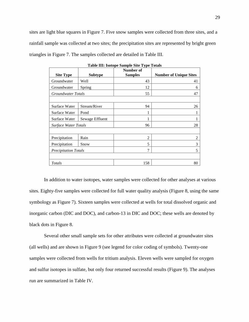
sites are light blue squares in Figure 7. Five snow samples were collected from three sites, and a
rainfall sample was collected at two sites; the precipitation sites are represented by bright green
triangles in Figure 7. The samples collected are detailed in Table III.
Table III: Isotope Sample Site Type Totals
Site Type Subtype
Number of
Samples Number of Unique Sites
Groundwater Well 43 41
Groundwater Spring 12 6
Groundwater Totals 55 47
Surface Water Stream/River 94 26
Surface Water Pond 1 1
Surface Water Sewage Effluent 1 1
Surface Water Totals 96 28
Precipitation Rain 2 2
Precipitation Snow 5 3
Precipitation Totals 7 5
Totals 158 80
In addition to water isotopes, water samples were collected for other analyses at various
sites. Eighty-five samples were collected for full water quality analysis (Figure 8, using the same
symbology as Figure 7). Sixteen samples were collected at wells for total dissolved organic and
inorganic carbon (DIC and DOC), and carbon-13 in DIC and DOC; these wells are denoted by
black dots in Figure 8.
Several other small sample sets for other attributes were collected at groundwater sites
(all wells) and are shown in Figure 9 (see legend for color coding of symbols). Twenty-one
samples were collected from wells for tritium analysis. Eleven wells were sampled for oxygen
and sulfur isotopes in sulfate, but only four returned successful results (Figure 9). The analyses
run are summarized in Table IV.

30
Figure 8: Sites of Water Quality and Carbon Suite Samples
Table IV: Summary of Water Analyses
Analysis Performed Groundwater Surface Water Precipitation Total Samples
Water Isotopes 55 96 7 158
Water Quality Suite 45 39 1 85
Carbon Suite 16 0 0 16
Tritium 21 0 0 21
Sulfur Isotopes* 11 0 0 11
*Only four samples yielded results.

31
Figure 9: Sites of Tritium, Field Sulfide, and Sulfur Isotope Samples (All Groundwater)
Water parameters measured when each sample was taken include: pH, temperature (°C),
specific conductance (SC, µS/cm), and dissolved oxygen (DO, mg/L). Measurements were taken
with either a YSI Professional or WTW water meter, calibrated before each field visit. The few
samples where water parameters were not recorded were due to either a lack of a water quality
meter (spur of the moment sampling, or equipment issues), or not enough available water to
cover the probe (as was the case for several of the precipitation samples).
Several analyses were performed in the field using Hach water quality testing kits and
reagents. An alkalinity titration was performed at sites where a carbon sample was collected, in
32
case verification of laboratory results was needed. The titration was done using a Hach Digital
Titrator, with a sulfuric acid cartridge and bromcresol-methyl red indicator powder. At wells
where the water had a distinct hydrogen sulfide gas odor (or where such an odor had been
previously reported), a Hach DR/700 colorimeter was used to measure the concentration of total
sulfide in the water.
All samples taken during this period adhered to the same collection procedures. Nitrile
gloves were worn from the beginning to the end of each collection to minimize skin oil
contamination of the samples. Standard wells not in frequent use were pumped to purge three
well volumes before samples were collected, to ensure the water sample was representative of
the water in the aquifer, not the stagnant water in the well casing. Wells in frequent use were
pumped for three well volumes or until water field parameters (temperature, pH, SC) stabilized.
Artesian well samples, spring samples, and surface water samples were collected via bucket,
after rinsing a clean sampling bucket three times in the sample water before collection. All
sample bottles and bottle caps were rinsed in the sample water three times before they were
filled, treated (when necessary) and sealed. Water was pumped into the sample bottles either
directly from the well, or by using a peristaltic pump in the case of bucket grab samples.
A 0.45 micron filter was used where filtering was required; this is the standard filter size used by
the MBMG for water sampling.
For each isotope sample, a 20-mL bottle of raw, untreated water was collected, and
tightly sealed with no headspace or air bubbles in the bottle to prevent air exchange with the
water. When the isotope sample was collected as part of a full water quality suite, the water was
filtered; when an isotope sample was the only bottle collected, it was left unfiltered and marked
as such so it would be filtered in the lab. Two duplicate samples were collected.

33
For each water quality analysis, four bottles of water were collected: a 500-mL bottle
filled with raw (unfiltered) water, a 250-mL bottle filled with filtered, raw water, a 500-mL
bottle with 5 mL of 15.8M nitric acid (HNO3 (aq)) and filtered water to full, and a 250-mL bottle
with 2.5 mL of 0.5M sulfuric acid (H2SO4 (aq)) and filtered water to full. Duplicate samples
were collected at two surface sites for water quality QA/QC.
Untreated, filtered water was collected for carbon isotopes in a 40-mL glass bottle with
no headspace or air bubbles, and sealed with a membrane cap.
For tritium analysis, two 500-mL bottles of raw, untreated water were collected, with no
headspace or bubbles. The caps on the bottles were also taped shut to provide a tight seal and
prevent air exchange during sample storage and transport to the lab.
To measure sulfur and oxygen isotopes in sulfate, a 500-mL bottle was filled with filtered
water and preserved with nitric acid. At sites where the field-measured sulfide concentration was
greater than or equal to 0.1 mg/L, a gallon of filtered water was collected and treated with 1 mL
of a dilute (10,000 ppm) silver nitrate (AgNO3 (aq)) solution to later measure sulfur isotopes in
sulfide.
All sample bottles were stored in insulated coolers with ice while in the field, and later
under refrigeration, until they were submitted to their respective labs for processing.
3.2. Analytical Methods
Water chemistry, oxygen-18, and deuterium analyses were performed by the MBMG
Analytical Laboratory. Major anions – bromide, chloride, fluoride, nitrate as nitrogen, nitrite as
nitrogen, orthophosphate as phosphorus, and sulfate – were analyzed by two Metrohm Ion
Chromatographs (IC), using EPA Method 300.0. Both ICs are calibrated with every sample run,
and quality control (QC) samples are analyzed according the EPA Method 300.0 as well.

34
Metals and trace elements were analyzed by a Thermo Scientific iCAP 6000 series
Inductively Coupled Plasma Optical Emission Spectroscope (ICP-OES) and a Thermo Scientific
iCAP-Q Inductively Coupled Plasma Mass Spectroscope (ICP-MS). The ICP-OES was used
primarily for major cations and higher metal/element concentrations, according to EPA Method
200.7. The ICP-MS detects trace elements and lower concentrations, running EPA Method
200.8. Both ICPs are calibrated every run and QC samples are analyzed according to the EPA
method.
A Metrohm robotic titrator with potentiometric assembly and auto sampler was used to
analyze alkalinity (by EPA Method 310.1), pH (EPA Method 150.1), and SC (EPA Method
120.1) in the laboratory. Water isotopes were analyzed using a Picarro L21030-i Cavity Ring-
Down Spectrometer (CRDS).
Carbon isotopes were analyzed in the MBMG lab with the assistance of Dr. Stephen
Parker. Concentrations of both dissolved inorganic carbon and dissolved organic carbon were
measured using an O•I Analytical Aurora Model 1030, while δ13C values in both DIC and DOC
were measured using a Picarro G2131-I CRDS for Isotopic CO2. The analyses were performed
by first running a portion of the sample for DIC and δ13C in DIC, then DOC and δ13C in DOC.
The initial run for DIC returned suspiciously high values, close to what Dr. Parker had
personally seen returned from samples in coalbed methane areas. The DIC analysis was repeated,
yielding different results. To determine which set of results was more accurate, the field
alkalinity, pH, and temperature for each sample were entered into geochemical modeling
program CO2-SYS to model total inorganic carbon based on the field data. CO2-SYS was run
with the data set in two independent trials. For both trials, the resulting carbon concentrations

35
more closely matched the concentrations from the second run of the samples; therefore those
data were kept for further analysis. The DOC analysis was performed only once.
3.2.1. Sulfur/Sulfate Samples
A 500-mL water sample, preserved with nitric acid, was collected from eleven wells for
the purpose of measuring δ34S and δ18O in sulfate. Unfortunately, the nitric acid used to preserve
the samples was too concentrated, and the pH of each sample dropped very low. As a result, the
initial lab processing of adding barium chloride to the sample and filtering out the resultant
barium sulfate precipitate for further analysis failed on all but three samples, even after adding
sodium hydroxide (NaOH) to the samples in an attempt to raise the pH.
Similarly, the samples for measuring total sulfide were not collected or treated correctly
in the field. One milliliter of the dilute silver nitrate solution in a gallon of water produced
essentially no silver sulfate precipitate. To get a measureable silver sulfide precipitate, less water
should have been collected (no more than a liter) and more silver nitrate should have been added.
As it was, only one sample produced enough precipitate to filter out and collect on filter papers
for processing, and that was only after adding more silver nitrate in the lab.
The four filter papers were sent to Dr. Simon Poulson at the University of Reno, Nevada,
for analysis at the Nevada Stable Isotope Lab. The lab uses two Micromass Isoprime stable
isotope mass spectrometers for their isotope analyses. Poulson was able to measure both δ34S and
δ18O values from one of the barium sulfate filter papers. The silver sulfide filter paper and the
other two barium sulfate filter papers could only provide sulfur-34 values.

36
3.2.2. Tritium Samples
The tritium samples were sent to the Environmental Isotopes Laboratory at the University
of Waterloo (uwEILAB), Toronto, Ontario, Canada, for analysis. The ewEILAB uses three LBK
Wallac 1220 Quantulus Liquid Scintillation Counters for enriched tritium measurement.

37
4. Results
4.1. Laboratory Results
4.1.1. Oxygen-18 and Deuterium
Oxygen-18 concentrations from the 158 samples analyzed ranged from -25.1‰ to
-13.6‰. Deuterium concentrations ranged from -184.0‰ to -100.0‰. For both oxygen-18 and
deuterium, the most enriched value came from a rainfall sample, and the most depleted came
from a snow sample. Groundwater samples ranged from -20.7‰ to -18.0‰ for oxygen-18 and
-158.0‰ to -139.0‰ for deuterium, while surface water samples ranged from -21.9‰ to -15.3‰
for oxygen-18 and -156.0‰ to -131.0‰ for deuterium (see Appendix C).
Oxygen-18 and deuterium results from the precipitation samples were plotted first, with
deuterium on the y-axis vs. oxygen-18 on the x-axis, as is convention. The trendline of these
samples forms a local meteoric water line (LMWL), showing a relationship between oxygen-18
and deuterium that all terrestrial waters in the region should follow (Figure 10). This LMWL for
Big Sky was compared to both the global meteoric water line (GMWL, determined by Craig,
1961) of:
δD = ((8 ∙ δ O18 ) + 10) (5)
and the Butte LMWL (Gammons et al., 2006) of:
δD = ((7.3 ∙ δ O18 ) − 7.5) (6)
As shown in Figure 10, the trendline for the Big Sky precipitation data yields a relationship of:
δD = ((7.17 ∙ δ O18 ) − 7.02) (7)

38
Figure 10: Plot of Preliminary Big Sky Local Meteoric Water Line (LMWL)
The local meteoric water line derived from the plot of the water isotope values from the
precipitation samples was reasonably close to both the GMWL and the Butte LMWL. With the
small set of precipitation data, compared to the sets in the studies by Craig and Gammons, this
Big Sky LMWL should be considered only preliminary, and as such will rarely be referenced
beyond this section.
The groundwater and surface water isotope samples were then added to the plot
(Figure 11). Rainwater should plot as the most isotopically enriched, snow as the most
isotopically depleted, with terrestrial waters in the middle, all roughly along the LMWL. The Big
Sky data generally followed this convention, as shown in Figure 11. These are all indications that
the sample results are accurate.
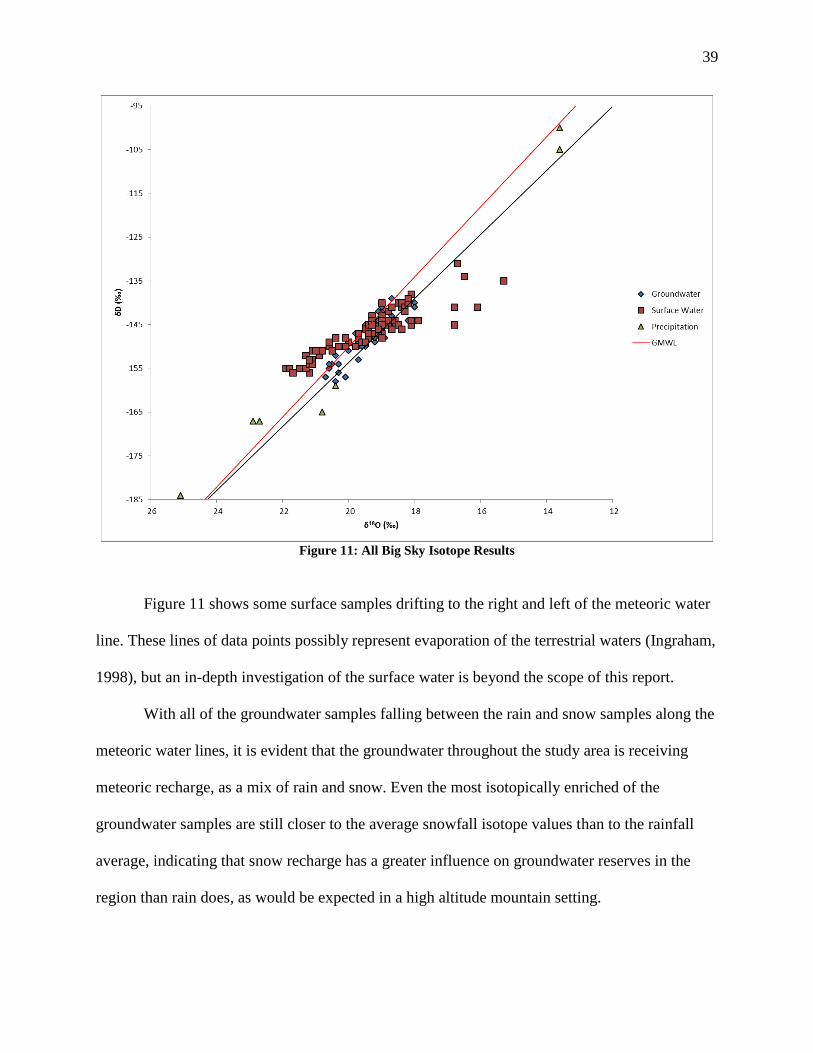
39
Figure 11: All Big Sky Isotope Results
Figure 11 shows some surface samples drifting to the right and left of the meteoric water
line. These lines of data points possibly represent evaporation of the terrestrial waters (Ingraham,
1998), but an in-depth investigation of the surface water is beyond the scope of this report.
With all of the groundwater samples falling between the rain and snow samples along the
meteoric water lines, it is evident that the groundwater throughout the study area is receiving
meteoric recharge, as a mix of rain and snow. Even the most isotopically enriched of the
groundwater samples are still closer to the average snowfall isotope values than to the rainfall
average, indicating that snow recharge has a greater influence on groundwater reserves in the
region than rain does, as would be expected in a high altitude mountain setting.

40
The concentrations of oxygen-18 and deuterium in the Big Sky terrestrial water samples
were well within the ranges found in Craig’s research (1961), and the way the snow and rain
isotope values act as endcaps for the groundwater and surface water samples also indicates good
quality samples and lab results.
Two duplicate isotope samples were sent to ewEILAB in Toronto for comparison to the
MBMG lab results. Results from both labs are summarized in Table V. (See map in Appendix A
for site locations.)
Table V: Differences in Lab Results for Two Isotope Samples
GWIC
ID
Site
Location
MBMG
δ18O (‰)
Waterloo
δ18O (‰)
Diff.
(‰)
MBMG
δD (‰)
Waterloo
δD (‰)
Diff.
(‰)
244347 Cascade #6 - Well
Mountain
Village -19.4 -19.1 0.3 -146.0 -143.5 2.5
283861 Buck’s T4 - Rain Isolated -13.6 -12.1 1.5 -105.0 -95.0 10.0
Wassenaar et al. (2012) recommended for isotope results from different labs or
equipment runs, oxygen-18 results should be within ±0.2‰, and deuterium within ±2‰. All of
the ewEILAB results are more enriched than the MBMG results, the rainfall sample by
1.5‰ oxygen-18 and 10.0‰ deuterium, and the groundwater sample by 0.3‰ oxygen-18 and
2.5‰ deuterium.
Both samples are out of the acceptable range of error, though the groundwater sample is
very close to meeting acceptance. The duplicate samples were stored under refrigeration for eight
months before being sent to ewEILAB for analysis, so it is quite possible that the initial tight
seals loosened during that time, allowing evaporation (leaving the samples more isotopically
enriched with respect to both oxygen-18 and deuterium). Lab error is also possible. Considering
how well the data set follows the meteoric water lines and follows expected conventions, these
two duplicate samples are not enough evidence to suggest that the data are anything but accurate.

41
4.1.2. DIC, DOC, and Carbon-13
Carbon analysis showed that the overwhelming majority of carbon present in the
collected samples was inorganic. DIC concentrations ranged from 21.9 to 130.6 mg/L, while
DOC ranged from just 0.3 to 2.8 mg/L (with two wells below the detection limit for DOC of
0.2 mg/L). Total dissolved carbon ranged from 22.2 to 131.6 mg/L. Carbon-13 in DIC ranged
from -14.5‰ to -6.3‰, and carbon-13 in DOC ranged from -38.6‰ to -21.9‰. The carbon
results are summarized in Table VI, along with pH. (See map in Appendix A for site locations.)
Table VI: Summary of Carbon Suite Results, plus pH Values
GWIC
ID Location Aquifer pH
DIC
(mg/L)
δ13C-DIC
(‰) DOC
mg/L
δ13C-DOC
(‰)
Total
DC
(mg/L)
103496 Mountain Village Dacite 9.5 21.9 -14.5 0.3 -34.3 22.2
176327 Yellowstone Club Morrison 7.7 34.6 -9.5 2.8 -23.9 37.4
192966 Yellowstone Club Kootenai 7.5 73.5 -9.1 0.3 -22.6 73.8
205931 Mountain Village Dacite 8.0 56.2 -6.9 0.2 -38.6 56.4
230689 Moonlight Basin Muddy 7.9 36.2 -13.0 0.4 -22.0 36.6
237292 Spanish Peaks Kootenai 7.7 53.9 -7.0 BDL BDL 53.9
239759 Spanish Peaks Kootenai 7.6 27.0 -11.8 0.1 -32.2 27.1
244347 Mountain Village Muddy 9.5 28.3 -13.8 0.5 -31.8 28.8
253676 Yellowstone Club Morrison 9.2 130.6 -6.3 1.0 -25.0 131.6
259357 Moonlight Basin Muddy 9.2 32.3 -13.1 0.4 -27.0 32.7
259685 Moonlight Basin Muddy 9.5 59.2 -7.4 BDL BDL 59.2
259706 Moonlight Basin Muddy 8.8 58.1 -13.5 0.6 -22.2 58.7
275582 Isolated (Uplands) Muddy 8.4 98.1 -11.6 1.7 -21.9 99.8
281359 Meadow Village Alluvium 7.6 69.4 -13.0 0.5 -23.2 69.9
281363 Meadow Village Alluvium 7.7 54.2 -11.9 0.6 -23.4 54.8
281366 Meadow Village Alluvium 7.5 57.2 -12.5 1.4 -23.7 58.6
Both DIC and DOC concentrations varied widely over the study area, as did the values of
δ13C within each. Of the sixteen samples, ten had δ13C in DIC values less than -10‰, indicating
soil-zone carbon dioxide as the primary carbon source. Not surprisingly, this included the three
wells sampled in the alluvial aquifer and five of six Muddy Sandstone wells, where carbonate
rocks would not be expected.

42
The remaining six samples had δ13C in DIC values between 0 and -10‰, a sign of
carbonate rocks as the most prominent carbon source. Both Morrison Formation wells were in
this range. The Morrison Formation and the Kootenai Formation above it contain some
freshwater limestone that would account for that carbon result. Dissolved organic carbon
concentrations were very low in the collected samples, with an average concentration of
0.8 mg/L, and a maximum concentration of 2.8 mg/L. While this is in stark contrast to the DIC
concentrations, DOC is typically low in groundwater because it is consumed by heterotrophic
microbes and converted to CO2 (Eby, 2004). The average expected DOC concentration for
groundwater overall is 0.7 mg/L (Eby, 2004), so the results are reasonable. By aquifer type, the
expected average for igneous rock aquifers is 0.5 mg/L; 0.7 mg/L for sand and gravel, limestone,
and sandstone aquifers; and 3.0 mg/L for oily shale aquifers (Eby, 2004). The four wells with
DOC concentrations greater than 1.0 mg/L all show some shale in their stratigraphy.
For aesthetic reasons (primarily color), DOC concentrations in drinking water should be
no more than 5-10 mg/L (Wang et al., 1998). Based on that standard, DOC is not the cause of
any water quality issues in the study area. However, other nations have different standards for
DOC in water; Finland, for example, states that DOC begins affecting aesthetics at
concentrations as low as 2 mg/L (Kortelainen and Karhu, 2006). Only one well sampled would
be above this standard – the Yellow Mule well (253676) in Yellowstone Club.
Of the fourteen samples with DOC above detection limits, seven had δ13C in DOC values
less than -24‰, the signature of vascular plant matter and microbial biomass sources providing
the DOC to the water. Unfortunately, the other constituent concentration needed to determine
which were from vascular plant matter and which were from microbial biomass, nitrogen, was
not above detection limits for any of the seven wells. Of the remaining seven samples, five were
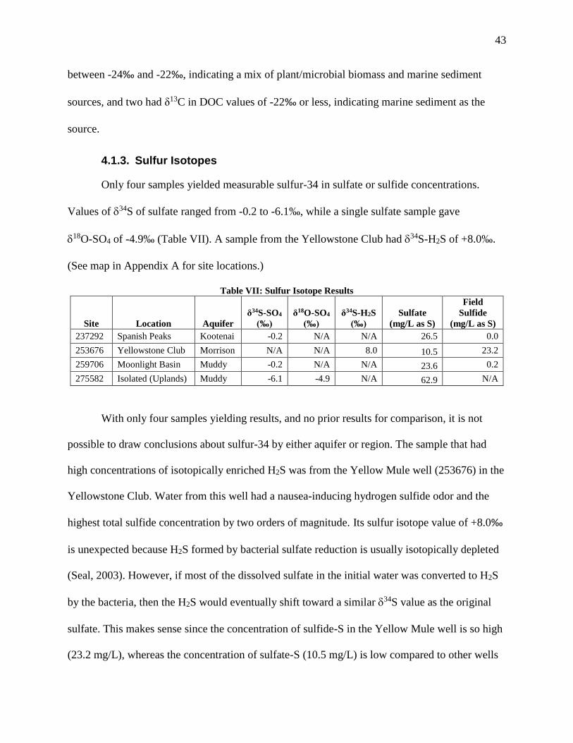
43
between -24‰ and -22‰, indicating a mix of plant/microbial biomass and marine sediment
sources, and two had δ13C in DOC values of -22‰ or less, indicating marine sediment as the
source.
4.1.3. Sulfur Isotopes
Only four samples yielded measurable sulfur-34 in sulfate or sulfide concentrations.
Values of 34S of sulfate ranged from -0.2 to -6.1‰, while a single sulfate sample gave
18O-SO4 of -4.9‰ (Table VII). A sample from the Yellowstone Club had 34S-H2S of +8.0‰.
(See map in Appendix A for site locations.)
Table VII: Sulfur Isotope Results
Site Location Aquifer
δ34S-SO4
(‰)
δ18O-SO4
(‰)
δ34S-H2S
(‰)
Sulfate
(mg/L as S)
Field
Sulfide
(mg/L as S)
237292 Spanish Peaks Kootenai -0.2 N/A N/A 26.5 0.0
253676 Yellowstone Club Morrison N/A N/A 8.0 10.5 23.2
259706 Moonlight Basin Muddy -0.2 N/A N/A 23.6 0.2
275582 Isolated (Uplands) Muddy -6.1 -4.9 N/A 62.9 N/A
With only four samples yielding results, and no prior results for comparison, it is not
possible to draw conclusions about sulfur-34 by either aquifer or region. The sample that had
high concentrations of isotopically enriched H2S was from the Yellow Mule well (253676) in the
Yellowstone Club. Water from this well had a nausea-inducing hydrogen sulfide odor and the
highest total sulfide concentration by two orders of magnitude. Its sulfur isotope value of +8.0‰
is unexpected because H2S formed by bacterial sulfate reduction is usually isotopically depleted
(Seal, 2003). However, if most of the dissolved sulfate in the initial water was converted to H2S
by the bacteria, then the H2S would eventually shift toward a similar 34S value as the original
sulfate. This makes sense since the concentration of sulfide-S in the Yellow Mule well is so high
(23.2 mg/L), whereas the concentration of sulfate-S (10.5 mg/L) is low compared to other wells

44
in the area. In other words, the sulfates in the vicinity of this pocket of groundwater have largely
been reduced to sulfide.
4.1.4. Tritium Samples
Of the 21 tritium samples (summarized in Table VIII), three had results of 0.8 TU or less,
indicating water older than the bomb pulse (according to the 1997 Clark and Fritz scale). Three
had values between 0.8 and 4.0 TU, representing a mix of pre-pulse and post-pulse waters. Three
samples had concentrations just over 4.0 TU, so they could be mixes or modern waters. The
remaining 12 samples all had concentrations between 4.0 and 15.0 TU, indicative of modern
(5 to 10 years old) waters. (See map in Appendix A for site locations.)
Table VIII: Tritium Results
GWICID Area Aquifer Tritium (TU) Age Category
215507 Moonlight Basin Muddy 6.4 Modern
230689 Moonlight Basin Muddy 6.3 Modern
230803 Mountain Village Muddy 7.3 Modern
259357 Moonlight Basin Muddy 4.1 Mix/Modern
259685 Moonlight Basin Muddy <0.8 Old
259706 Moonlight Basin Muddy 0.9 Mix
279062 Moonlight Basin Frontier 6.4 Modern
279080 Moonlight Basin Dacite 7.3 Modern
230804 Moonlight Basin Muddy <0.8 Old
275582 Isolated Muddy 2.5 Mix
219966 Spanish Peaks Morrison 4.3 Mix/Modern
237292 Spanish Peaks Kootenai 5.0 Modern
176327 Yellowstone Club Morrison 6.7 Modern
192966 Yellowstone Club Kootenai 5.1 Modern
253676 Yellowstone Club Morrison <0.8 Old
281363 Meadow Village Alluvium 6.2 Modern
281371 Meadow Village Alluvium 5.6 Modern
205931 Mountain Village Dacite 6.1 Modern
239759 Spanish Peaks Kootenai 2.0 Mix
103496 Mountain Village Dacite 4.2 Mix/Modern
244347 Mountain Village Muddy 6.5 Modern
45
GWCP collected samples for tritium analysis prior to this study. In the GWCP samples,
tritium values ranged from 0.8 TU to 12.3 TU, still within the same age ranges as in this project.
One well from the previous work was resampled in this study, to compare sampled results to
separate sample sources and expand the dataset. Well 244347, the Cascade #6 well in Mountain
Village, had a tritium concentration of 2.7 TU when tested in 2011; it now has a concentration of
6.5 TU, possibly indicating the well is now predominantly recharged by modern water.
4.1.5. Water Quality
Water quality analyses results were compared to the EPA standards for drinking water,
irrigation water, and stock water. Primary standards are for issues of health, while secondary
standards are for aesthetic reasons – such as taste, odor, or color – that are not harmful, but
render the water undesirable for use. Among the 85 samples, primary exceedances were very
few, but secondary exceedances were common. There were also several exceedances for
irrigation water and stock water. The exceedances – primary, secondary, and otherwise – are
summarized in Table IX. (Water quality results can be found in Appendices D, E, and F; site
locations can be found on the map in Appendix A.)
From this analysis it appears that most water in the Big Sky study area is safe for
drinking from a health-threat standpoint. Only two wells in this sample set exceeded primary
health standards – one for arsenic (well 244347, the Cascade #6 well in Mountain village), and
one for fluoride (well 259357, a golf course test well in Moonlight Basin). However, many more
wells exceed secondary standards, some greatly exceeding, meaning the water has a bad taste or
odor, or is discolored. Additionally, many samples were determined to be hard or very hard
water, which is also undesirable.

46
Table IX: Summary of Water Quality Exceedances
Number of Exceedances
Constituent Type of Standard Limit Groundwater Surface Water
Sewage
Effluent
Drinking Water
Arsenic Primary 10 µg/L 1 0 0
Fluoride Primary 4 mg/L 1 0 0
Sodium WHO 200 mg/L 2 0 0
Elevated 15 mg/L 20 0 1
Chloride Elevated 15 mg/L 15 4 1
Iron Secondary 0.3 mg/L 1 0 0
Manganese Secondary 0.05 mg/L 8 0 0
Aluminum Secondary 50 µg/L 0 10 0
Sulfate Secondary 250 mg/L 1 0 0
pH Secondary 6.5-8.5 10 4 0
TDS Secondary 500 mg/L 5 0 0
Hardness Hard 121-180 mg/L 6 8 1
Very Hard 180 mg/L+ 18 1 0
Irrigation Water
Molybdenum 5 µg/L 4 0 1
SAR Medium Risk 10+ 2 0 0
High Risk 18+ 5 0 0
Stock Water
Fluoride 2 mg/L 3 0 0
Several wells exceeded standards for irrigation. While there is currently no agriculture in
the Big Sky area, a great deal of landscaping has been done at both businesses and homes, and
there are numerous golf courses that require frequent watering. Four wells – 259706, the
Moonlight Basin Golf Course well; 219966, the Spanish Peaks Entrance Gate well; 176326, the
Equine Center well in Yellowstone Club; and 275582, the Uplands well isolated south of
Meadow Village – plus the Big Sky Water and Sewer District treated effluent exceeded the
standard for molybdenum. Most notable is the sewage effluent, which is primarily used for
watering the Meadow Village golf course. It is four times the recommended limit for

47
molybdenum in irrigation water. Plants watered with high-molybdenum irrigation water are not
safe for livestock to consume. While this water is only used on the golf course, wild deer and
moose are known to wander the area and presumably eat some of the grass. Whether deer and
moose are affected by molybdenum in the same way as cattle is not known, and may be worth
further study. The other four wells are not used for irrigation at this time.
Additionally, water samples from seven wells had SAR values that pose a medium to
high risk to soil structure when used for extended periods of irrigation. Two of the high risk
wells are in Moonlight Basin: 230804, the Lee’s Pool well, and 259685, the golf course test well.
The Cascade #6 well (244347) in adjacent Mountain Village poses medium risk, as does the
Spanish Peaks Entrance Gate well (219966). The laundromat well in Meadow Village (104510)
poses high risk, as do the Yellow Mule well (253676) in Yellowstone Club and the isolated
Uplands well (275582).
There are three exceedances of the stock water regulation for fluoride. Cattle ranching no
longer occurs in the Big Sky area, but there are several businesses providing horseback riding
tours in the region, and there are large corrals in Moonlight Basin, Spanish Peaks, and the
Yellowstone Club. Luckily, these wells – 259357, a golf course test well in Moonlight Basin;
262271, the American Spirit well in Yellowstone Club; and 253676, the Yellow Mule well in
Yellowstone Club – are not being used to supply water at any of the horse corrals.
While only two wells were over the WHO objective of 200 mg/L for sodium (the Yellow
Mule and Uplands wells), and none exceeded the EPA secondary standard of 250 mg/L for
chloride, there were numerous wells with elevated concentrations of sodium and chloride, greater
than 15 mg/L. These elevated levels may indicate an anthropogenic source of the ions, if marine
shales are not present. Long et al. (2015) noted that a common source of elevated sodium and

48
chloride in groundwater is deicing salt applied to roadways during the winter months, which
would explain elevated levels in Meadow Village especially. In addition, sixteen wells have a
sodium concentration of 20 mg/L or higher, which is often enough to affect the aesthetic quality
of the water (WHO, 1996).
None of the groundwater samples were above the EPA standard for nitrate of 10 mg/L.
The average nitrate concentration in groundwater was 1.1 mg/L, with the highest concentrations
in the alluvial aquifer in Meadow Village. The average nitrate concentration in surface water was
0.2 mg/L. (See Appendix E for details.)
4.1.6. Water Types
Water quality analyses results were imported into AquaChem for determination of water
type. The water type is determined by converting concentrations of all ions to meq/L, then to
meq%. All parameters below 10% are removed, leaving only the major ions for that particular
sample. The major cations are ordered from highest percentage to lowest, then the major anions
are ordered in the same fashion to create the water type string (e.g., calcium-magnesium
bicarbonate-sulfate). Water types can also be described in a short string, which describes only the
most abundant cation and most abundant anion (e.g., calcium bicarbonate).
By the short-string description, there are two primary water types in Big Sky: calcium
bicarbonate and sodium bicarbonate. Of the 85 water quality samples, 72 were calcium
bicarbonate waters and 13 were sodium bicarbonates.
Of the 45 groundwater samples (wells and springs), 33 were calcium bicarbonates and
12 were sodium bicarbonates. The specific water types varied widely. The most common water
type was calcium-magnesium bicarbonate with 13 occurrences. The second most frequent was
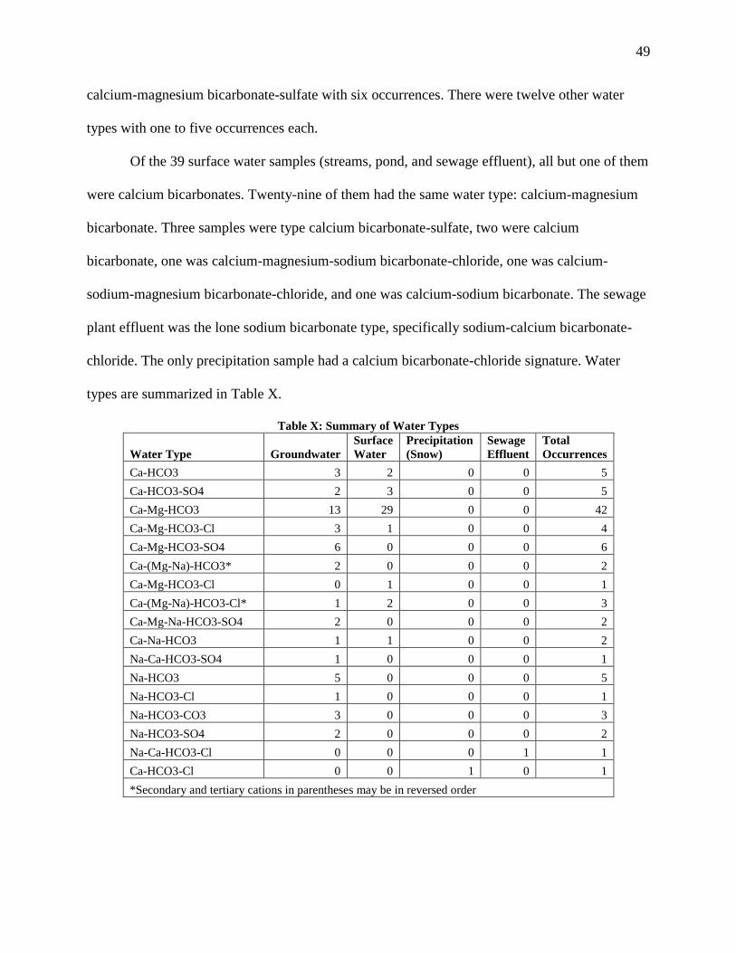
49
calcium-magnesium bicarbonate-sulfate with six occurrences. There were twelve other water
types with one to five occurrences each.
Of the 39 surface water samples (streams, pond, and sewage effluent), all but one of them
were calcium bicarbonates. Twenty-nine of them had the same water type: calcium-magnesium
bicarbonate. Three samples were type calcium bicarbonate-sulfate, two were calcium
bicarbonate, one was calcium-magnesium-sodium bicarbonate-chloride, one was calcium-
sodium-magnesium bicarbonate-chloride, and one was calcium-sodium bicarbonate. The sewage
plant effluent was the lone sodium bicarbonate type, specifically sodium-calcium bicarbonate-
chloride. The only precipitation sample had a calcium bicarbonate-chloride signature. Water
types are summarized in Table X.
Table X: Summary of Water Types
Water Type Groundwater
Surface
Water
Precipitation
(Snow)
Sewage
Effluent
Total
Occurrences
Ca-HCO3 3 2 0 0 5
Ca-HCO3-SO4 2 3 0 0 5
Ca-Mg-HCO3 13 29 0 0 42
Ca-Mg-HCO3-Cl 3 1 0 0 4
Ca-Mg-HCO3-SO4 6 0 0 0 6
Ca-(Mg-Na)-HCO3* 2 0 0 0 2
Ca-Mg-HCO3-Cl 0 1 0 0 1
Ca-(Mg-Na)-HCO3-Cl* 1 2 0 0 3
Ca-Mg-Na-HCO3-SO4 2 0 0 0 2
Ca-Na-HCO3 1 1 0 0 2
Na-Ca-HCO3-SO4 1 0 0 0 1
Na-HCO3 5 0 0 0 5
Na-HCO3-Cl 1 0 0 0 1
Na-HCO3-CO3 3 0 0 0 3
Na-HCO3-SO4 2 0 0 0 2
Na-Ca-HCO3-Cl 0 0 0 1 1
Ca-HCO3-Cl 0 0 1 0 1
*Secondary and tertiary cations in parentheses may be in reversed order

50
In addition to the water type assignments, AquaChem was also utilized to create Piper
diagrams and Stiff diagrams. A Piper diagram is a trilinear plot that displays the concentrations
of the major ions all at once. The cations are organized on one triangular plot (with Na+ and K+
together on one side), the anions on another (with carbonate and bicarbonate together on one
side), and a rhombus-shaped plot between them summarizes the composition of the water
relative to both major cations and anions. Two Piper plots were created: one for the groundwater
samples (Figure 12), and one for the surface water and precipitation samples (Figure 13).

51
Figure 12: Piper Diagram for Groundwater Samples. Legend translation:
111SNGR = Alluvium/Sand and Gravel, 112RKGL = Rock Glacier, 211FRNR = Frontier Formation,
211PLNC = Dacite Sills, 217KOTN = Kootenai Formation, 217MDDY = Muddy Sandstone,
217MWRY = Mowry Shale, 221MRSN = Morrison Formation, 330MDSN = Madison Limestone Group.

52
Figure 13: Piper Diagram for Surface Water, Precipitation, and Effluent Samples
A Stiff diagram was created for each individual sample. Stiff diagrams are a good tool for
visual comparison of ion concentrations and water types among samples in the same
geographical area. They display major cations on the left of a center line, and major anions on
the right. Concentrations are plotted on the same scale going outward from a center line, and the
points are connected to form a shape. A quick glance at the Stiff diagrams from multiple samples
can give a rough idea of whether they have similar water types, based on the shape of the plot.

53
Because the majority of the samples were of a calcium bicarbonate water type, the Stiff
diagrams were created with calcium and bicarbonate+carbonate on the first horizontal line,
magnesium and sulfate on the second, and sodium+potassium and chloride on the third. In order
to draw accurate conclusions, all Stiff diagrams being compared must be on the same scale. Stiff
diagrams were analyzed in different groups (by aquifer, by region, etc.). A representative Stiff
diagram for the alluvium aquifer is shown in Figure 14. The Stiff diagrams for each water quality
sample are in Appendix G. All the Stiff diagrams – for groundwater and surface water alike – are
on the same scale for easy comparison.
Figure 14: Stiff Diagram for an Alluvial Well, Presented as a Representative Example
4.2. Field Analysis Results
Field results for pH, SC, and temperature for each sample can be found in Appendix C.
Field pH ranged from 5.2 (rain sample 283861) to 10.1 (230804, Lee’s Pool well,
screened in the Muddy Sandstone in the Moonlight Basin). Under the EPA secondary standards
for drinking water, the acceptable range for pH is 6.5 to 8.5. Nine wells had pH values exceeding
the upper limit of the acceptable range, and twenty-two of the surface water samples also had a

54
pH of 8.5 or higher (Appendix C). According to the EPA (2016), high pH water has an
unpleasant soda taste, a slippery feel, and can leave deposits similar to those from hard water,
making it undesirable for use. The rain sample was the only pH value below the bottom limit of
the acceptable range.
Field SC ranged from 2 (precipitation) to 1332 µS/cm (the Yellow Mule well, screened in
the Morrison Formation in Yellowstone Club). It would be expected for freshly fallen
precipitation to have an SC value of essentially zero. It is also unsurprising that the Yellow Mule
well, with water of visibly poor quality, would be the most mineralized. Specific conductance
can act as a rough age-dating mechanism as older water has gone through longer flowpaths and
interacted with more rock, becoming more mineralized with time.
Samples were taken at all times of year, so water temperatures unsurprisingly ranged
from -0.1°C to 17.5°C. The well samples had an average temperature of 6.6°C, with the coldest
at 3.1°C and the warmest at 11.1°C. There was not a correlation between either depth or time of
year with temperature.
A field alkalinity titration was performed at twelve of the sixteen wells where carbon
samples were collected. The titrated values ranged from 144.0 to 578.0 mg CaCO3/L (Table XI).
The field values were reasonable in comparison to the lab calculated alkalinity concentrations,
allowing for changes due to reactions occurring in the water while in transit and storage prior to
testing.
Total sulfide was measured at ten wells, where either a hydrogen sulfide gas odor was
detected at the time of sampling, or where an odor had been previously reported (Table XII).
Two of the field tests resulted in no measureable sulfide; seven wells had between
0.01 and 0.22 mg/L total sulfide. One well, however, had 23.15 mg/L total sulfide – the Yellow

55
Mule well in Yellowstone Club, which had a nearly overwhelming hydrogen sulfide odor.
Individual sulfide concentrations will be discussed further in the next section.
Table XI: Field Alkalinity Concentrations
GWIC ID Location Aquifer
Alkalinity
(mg/L CaCO3)
281359 Meadow Village Alluvium 252
281363 Meadow Village Alluvium 195
281366 Meadow Village Alluvium 205
192966 Yellowstone Club Kootenai 286
237292 Spanish Peaks Kootenai 185
176327 Yellowstone Club Morrison 147
253676 Yellowstone Club Morrison 578
230689 Moonlight Basin Muddy 162
259357 Moonlight Basin Muddy 144
259685 Moonlight Basin Muddy 263
259706 Moonlight Basin Muddy 252
275582 Isolated (Uplands) Muddy 408
Table XII: Field Sulfide Concentrations
GWIC ID Location Aquifer Sulfide (mg/L)
192966 Yellowstone Club Kootenai 0.06
215507 Moonlight Basin Muddy 0.00
230689 Moonlight Basin Muddy 0.01
230804 Moonlight Basin Muddy 0.22
237292 Spanish Peaks Kootenai 0.00
253676 Yellowstone Club Morrison 23.15
259357 Moonlight Basin Muddy 0.06
259685 Moonlight Basin Muddy 0.20
259706 Moonlight Basin Muddy 0.16
279062 Moonlight Basin Frontier 0.01

56
5. Analysis and Discussion
The discussion that follows will focus on separating the data by geologic unit/aquifer
(Section 5.1) and then by region (Section 5.2) to help characterize water signatures. The desired
outcome was to find connections in isotopes, age, and water chemistry and quality, whether by
unit, by region, or a combination of both.
The terms “aquifer” and “geologic unit” will be used interchangeably in this section,
though geologic unit is the more accurate of the two.
Many wells and spring sites are referenced by their GWIC IDs. While the map in
Appendix A shows the GWIC IDs for all the sites in the area, for closer details by aquifer and
region, see Figures 15, 16, and 17. For isotope and water quality results more specific than
described in the discussion, see Appendices C-F. For details on Stiff diagrams, see Appendix G.

57
Figure 15: Detailed map for Meadow Village Area. Topographic scale in feet.

58
Figure 16: Detailed map for Moonlight Basin and Mountain Village. Topographic scale in feet.

59
Figure 17: Detailed map for Yellowstone Club and Spanish Peaks. Topographic scale in feet.

60
5.1. Analysis by Aquifer
The groundwater sample sites selected for this study were completed or sourced from
nine different geologic units: alluvium, rock glacier, dacite sills, Frontier Formation, Mowry
Shale, Muddy Sandstone, Kootenai Formation, Morrison Formation, and the Madison Group. To
determine a unique isotopic/chemical signature to the water of each unit, data were sorted and
plotted by unit.
Groundwater isotope values sorted by geologic unit are shown in Figure 18. The average
values and standard deviations calculated for each unit are shown in Table XIII and in Figure 19,
with the rain and snow values for reference, and in Figure 20, the same data at a larger scale.
Figure 18: Groundwater Isotopes, by Geologic Unit

61
Table XIII: Water Isotope Values by Geologic Unit
Aquifer Average δ18O (‰) Standard Deviation Average δD (‰) Standard Deviation
Alluvium -18.7 0.3 -145.4 2.6
Rock Glacier -19.0 0.1 -143.7 1.3
Dacite -19.4 0.4 -145.0 3.8
Frontier -18.7 N/A -139.0 N/A
Mowry -19.4 0.5 -148.0 5.1
Muddy -19.8 0.5 -150.1 4.5
Kootenai -19.8 0.6 -151.2 4.5
Morrison -19.7 1.0 -150.2 6.7
Madison -19.6 0.3 -149.0 0.7
Figure 19: Average Water Isotope Values by Unit and Precipitation Source, with Standard Deviation

62
Figure 20: Average Water Isotope Values by Unit, with Standard Deviation
Carbon suite values, by unit, are shown in Tables XIV and XV. The data are represented
graphically by both carbon-13 vs. carbon concentration, and carbon-13 vs. inverse concentration
(Figures 21 and 22 for DIC, and Figures 23 and 24 for DOC). Tritium concentrations sorted by
aquifer are shown in Table XVI.

63
Table XIV: pH and Carbon Data by Unit
GWIC
ID Location Aquifer pH
DIC
(mg/L)
δ13C-DIC
(‰) DOC
mg/L
δ13C-DOC
(‰)
Total
DC
(mg/L)
281359 Meadow Village Alluvium 7.6 69.4 -13.0 0.5 -23.2 69.9
281363 Meadow Village Alluvium 7.7 54.2 -11.9 0.6 -23.4 54.8
281366 Meadow Village Alluvium 7.5 57.2 -12.5 1.4 -23.7 58.6
103496 Mountain Village Dacite 9.5 21.9 -14.5 0.3 -34.3 22.2
205931 Mountain Village Dacite 8.0 56.2 -6.9 0.2 -38.6 56.4
192966 Yellowstone Club Kootenai 7.5 73.5 -9.1 0.3 -22.6 73.8
237292 Spanish Peaks Kootenai 7.7 53.9 -7.0 BDL BDL 53.9
239759 Spanish Peaks Kootenai 7.6 27.0 -11.8 0.1 -32.2 27.1
176327 Yellowstone Club Morrison 7.7 34.6 -9.5 2.8 -23.9 37.4
253676 Yellowstone Club Morrison 9.2 130.6 -6.3 1.0 -25.0 131.6
230689 Moonlight Basin Muddy 7.9 36.2 -13.0 0.4 -22.0 36.6
244347 Mountain Village Muddy 9.5 28.3 -13.8 0.5 -31.8 28.8
259357 Moonlight Basin Muddy 9.2 32.3 -13.1 0.4 -27.0 32.7
259685 Moonlight Basin Muddy 9.5 59.2 -7.4 BDL BDL 59.2
259706 Moonlight Basin Muddy 8.8 58.1 -13.5 0.6 -22.2 58.7
275582 Isolated (Uplands) Muddy 8.4 98.1 -11.6 1.7 -21.9 99.8
Table XV: Average pH and Carbon Values by Unit
Geologic Unit pH DIC (mg/L) δ13C-DIC (‰) DOC (mg/L) δ13C-DOC (‰)
Alluvium Mean 7.6 60.3 -12.4 0.8 -23.4
Std Dev N/A 6.6 0.5 0.4 0.2
Dacite Mean 8.8 39.1 -10.7 0.3 -36.5
Std Dev N/A 17.2 3.8 0.1 2.2
Muddy Mean 8.9 52.0 -12.1 0.7 -25.0
Std Dev N/A 23.9 2.2 0.5 3.9
Kootenai Mean 7.6 51.4 -9.3 0.2 -27.4
Std Dev N/A 19.0 2.0 0.1 4.8
Morrison Mean 8.5 82.6 -7.9 1.9 -24.4
Std Dev N/A 48.0 1.6 0.9 0.6
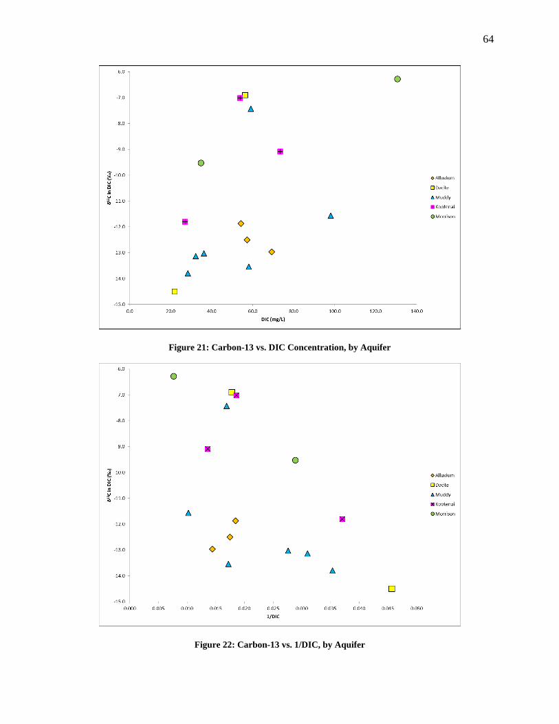
64
Figure 21: Carbon-13 vs. DIC Concentration, by Aquifer
Figure 22: Carbon-13 vs. 1/DIC, by Aquifer

65
Figure 23: Carbon-13 vs. DOC Concentration, by Aquifer
Figure 24: Carbon-13 vs. 1/DOC, by Aquifer
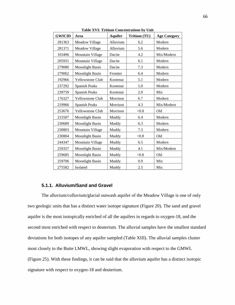
66
Table XVI: Tritium Concentrations by Unit
GWICID Area Aquifer Tritium (TU) Age Category
281363 Meadow Village Alluvium 6.2 Modern
281371 Meadow Village Alluvium 5.6 Modern
103496 Mountain Village Dacite 4.2 Mix/Modern
205931 Mountain Village Dacite 6.1 Modern
279080 Moonlight Basin Dacite 7.3 Modern
279062 Moonlight Basin Frontier 6.4 Modern
192966 Yellowstone Club Kootenai 5.1 Modern
237292 Spanish Peaks Kootenai 5.0 Modern
239759 Spanish Peaks Kootenai 2.0 Mix
176327 Yellowstone Club Morrison 6.7 Modern
219966 Spanish Peaks Morrison 4.3 Mix/Modern
253676 Yellowstone Club Morrison <0.8 Old
215507 Moonlight Basin Muddy 6.4 Modern
230689 Moonlight Basin Muddy 6.3 Modern
230803 Mountain Village Muddy 7.3 Modern
230804 Moonlight Basin Muddy <0.8 Old
244347 Mountain Village Muddy 6.5 Modern
259357 Moonlight Basin Muddy 4.1 Mix/Modern
259685 Moonlight Basin Muddy <0.8 Old
259706 Moonlight Basin Muddy 0.9 Mix
275582 Isolated Muddy 2.5 Mix
5.1.1. Alluvium/Sand and Gravel
The alluvium/colluvium/glacial outwash aquifer of the Meadow Village is one of only
two geologic units that has a distinct water isotope signature (Figure 20). The sand and gravel
aquifer is the most isotopically enriched of all the aquifers in regards to oxygen-18, and the
second most enriched with respect to deuterium. The alluvial samples have the smallest standard
deviations for both isotopes of any aquifer sampled (Table XIII). The alluvial samples cluster
most closely to the Butte LMWL, showing slight evaporation with respect to the GMWL
(Figure 25). With these findings, it can be said that the alluvium aquifer has a distinct isotopic
signature with respect to oxygen-18 and deuterium.

67
Figure 25: Water Isotopes in Alluvium Aquifer
With the West Fork of the Gallatin River and its tributary, Crail Creek, running through
the alluvium, some surface water interaction would be expected. On average, the alluvial
samples are similar to the surface samples, but are slightly more enriched, especially with respect
to oxygen-18. These results indicate that the alluvium experiences more rain recharge and
surface water interaction than the other geologic units.
Water tables generally follow the slopes of surface topography. As can be seen from
Figure 15, the alluvial sample sites are all located in the low basin of Meadow Village, with a
gentle decreasing slope from west to east. Water from the southern alluvial sites flows toward the
South Fork, while water from the other sites flows more directly to the West Fork.

68
In terms of carbon, the alluvium again had the closest to a distinct signature of all the
aquifers. DIC concentrations in the sand and gravel ranged from 54.2 to 69.4 mg/L, and DOC
from 0.5 to 1.4 mg/L. Carbon-13 in DIC ranged from -11.9‰ to -13.0‰, and δ13C in DOC
ranged from -23.2‰ to -23.7‰. These values would indicate that all the DIC in the alluvial
groundwater is derived from carbon dioxide gas in the soil, and all the DOC is a mix of plant
matter/microbial biomass and marine sediments (more heavily on the plant matter and microbial
biomass). The evidence of marine influence in an alluvial aquifer at first seems unusual. With
marine shales underlying the immediate region and making up much of the study area, it is not
unreasonable that some seepage from the surrounding shale aquifers is influencing the alluvial
groundwater.
Both of the tritium samples collected from the alluvial aquifer indicated modern water
(Table XVI). The aquifer is shallow and interacts with the local surface water, and precipitation
percolates through the aquifer for recharge, so modern-aged water is what would be expected.
The alluvium aquifer samples – ten from wells and two from springs – had the best
correlation among all samples in terms of water type of all the aquifers. They all exhibited a
calcium-magnesium bicarbonate water type, with some variation in secondary and tertiary anions
(Table XV). As can be seen in Appendix G, all the alluvial site Stiff diagrams are nearly
identical in shape, indicating the waters are very similar. Calcium-magnesium bicarbonate is also
the most common water type among the surface water samples, serving as further evidence of a
strong surface water influence in the alluvium aquifer. Van Voast (1972) found a dominant
calcium-magnesium bicarbonate water type in the alluvial aquifer. In Brown’s study (2014),
eighteen of twenty alluvium samples exhibited the calcium-magnesium bicarbonate type. The
fact that the overall water type in the alluvium has remained the same over a period of four

69
decades speaks to good waste management and environmental controls in the area, despite all the
development.
Table XVII: Water Types in the Alluvium Aquifer
GWIC ID Water Type
281360 Ca-Mg-HCO3
281362 Ca-Mg-HCO3
281363 Ca-Mg-HCO3
281366 Ca-Mg-HCO3
281367 Ca-Mg-HCO3
281368 Ca-Mg-HCO3
281371 Ca-Mg-HCO3
281372 Ca-Mg-HCO3
281373 Ca-Mg-HCO3
278297 Ca-Mg-HCO3-Cl
281359 Ca-Mg-HCO3-Cl
280689 Ca-Mg-Na-HCO3-Cl
The ten wells sampled in the alluvium were drilled by the MBMG (along with five other
wells) for use as monitoring wells. There were no primary or secondary drinking standard
exceedances in any of the wells, but eight of them had very hard water (hardness values of
180 mg/L or more), with a ninth having hard water (hardness between 121 and 180 mg/L). Two
of the wells and both of the springs had elevated sodium concentrations, but below the WHO
limit. Both of the springs also had very hard water, and one exceeded the TDS secondary
standard limit, but these are both low-volume springs that would not be useful as any sort of
water supply. The springs are also located downgradient of the Meadow Village, where the
alluvium drains into the South Fork Gallatin River. Elevated levels of chloride (greater than
15 mg/L) were found in eight of the wells, plus both springs. In previous studies, only two
secondary standard exceedances were found in the alluvium aquifer: Baldwin (1997) found a
single exceedance of pH, and Brown (2014) found one iron exceedance, with elevated chloride
in twelve of them.

70
While Baldwin (1997) had found many wells in the alluvium with high arsenic levels,
that was not the case in this study. The average arsenic concentration was 0.4 µg/L (with a
maximum value of 0.8 µg/L), well below the primary standard limit of 10 µg/L. It is possible
that there was a laboratory error with Baldwin’s analyses, as it is unlikely that a large amount of
arsenic could have simply disappeared from the region.
Values for pH in the alluvial samples were consistent; average pH was 7.6, with a
minimum of 7.4 and a maximum of 7.8. Nitrate values were higher in the alluvium than in any
other geologic unit. The average nitrate value was 2.4 mg/L. Three sites had significantly
elevated nitrate levels: spring 278297 (below American Bank) and well 281359 (MV14-1), both
at 4.9 mg/L, and well 281372 (MV14-12) at 6.3 mg/L. These three sites are all located at the
edge of or in the outwash area of the golf course (see Figure 15). The concern of increasing
nitrate levels from fertilizers and other treatments was the focus of the GWCP study, as well as
the McGlynn group research, and it would appear that they are still a concern in the area, despite
overall good environmental practices.
No sulfur isotope samples were collected from the alluvial aquifer. No hydrogen sulfide
odors were noted in the alluvium, so no field sulfide analyses were performed. Sulfate was low
in the aquifer, with an average concentration of 17.3 mg/L.
5.1.2. Rock Glacier
A rock glacier at the base of the ski runs in the Mountain Village area was the other
geologic unit that presented a unique water isotope signature (Figure 20); even though the
samples were all collected at the same spring site, they were collected at different times of the
year and have slightly different values, as seen in Figure 18. The rock glacier is composed of
broken dacite rock fragments up to one foot in length. The location of the rock glacier

71
(Figure 16) suggests it is recharged by overland snowmelt infiltration that has had a chance to
undergo slight evaporation (and become more enriched than pure snow) and perhaps some rain.
The spring was not tested for carbon/carbon isotopes, tritium, sulfur, or sulfide. It was
analyzed for water chemistry once and was shown to have a calcium-bicarbonate water type, but
there were no rock glacier sites analyzed in the prior study for comparison. Its SC value was only
63 µS/cm, which would indicate that it has not had much rock-water interaction and would
support the theory that it is recharged mostly by snowmelt. The quality of the rock glacier water
is excellent, with no primary or secondary standards exceeded. Its nitrate and sulfate
concentrations were very low, at 0.3 mg/L and 5.6 mg/L, respectively, and its average pH over
the course of three isotope samples was 7.9. Discharge from this particular spring is low, and it
does not produce enough volume to be utilized as any sort of water supply. Topography indicates
water from the area of the rock glacier will flow toward Mountain Village and the Middle Fork.
5.1.3. Dacite Sills
Four wells and one spring are completed or originate in dacite sills extending outward
from the core of Lone Peak. While they are grouped together for the analyses by aquifer, it is
important to note that the dacite is not a continuous layer. As can be seen in Figure 16, wells
103496 and 205931 are located northeast of Lone Peak, while wells 279080 and 279082 (not
shown, isotope sample only) and spring site 279079 are almost due north of the peak. It is likely
that these two sets of sites are in different sills. Additionally, the thick red line shown on
Figure 16 represents a watershed divide; water on the west side of the divide flows westward
along the topography to Jack Creek, while water on the east side flows southeastward along the
topography to the Middle Fork. The sets of dacite sample sites on either side of this divide are
receiving different recharge water and are not connected to each other after all.

72
Overall, the dacite wells and spring are on the more enriched end of the groundwater
spectrum with respect to both oxygen-18 and deuterium (Figure 20). They appear to be
recharged by snowmelt and rainfall. The samples are tightly grouped around the GMWL
(Figure 26); this would indicate that very little evaporation has occurred in the recharge water.
The range of values for both isotopes overlaps completely with the rock glacier groundwater, and
partially with several other bedrock aquifers. Despite being on opposite sides of the watershed
divide and in different sills, the four wells all had similar isotopic concentrations, especially with
respect to oxygen-18. The most isotopically enriched well samples came from 279080, which is
an artesian well. The spring samples were the most isotopically enriched of the samples, with
respect to both oxygen-18 and deuterium.
Figure 26: Water Isotopes in Dacite Sills
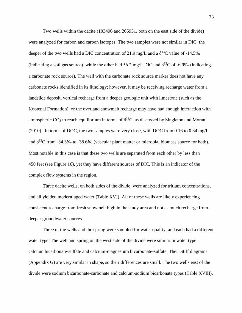
73
Two wells within the dacite (103496 and 205931, both on the east side of the divide)
were analyzed for carbon and carbon isotopes. The two samples were not similar in DIC; the
deeper of the two wells had a DIC concentration of 21.9 mg/L and a δ13C value of -14.5‰
(indicating a soil gas source), while the other had 56.2 mg/L DIC and δ13C of -6.9‰ (indicating
a carbonate rock source). The well with the carbonate rock source marker does not have any
carbonate rocks identified in its lithology; however, it may be receiving recharge water from a
landslide deposit, vertical recharge from a deeper geologic unit with limestone (such as the
Kootenai Formation), or the overland snowmelt recharge may have had enough interaction with
atmospheric CO2 to reach equilibrium in terms of δ13C, as discussed by Singleton and Moran
(2010). In terms of DOC, the two samples were very close, with DOC from 0.16 to 0.34 mg/L
and δ13C from -34.3‰ to -38.6‰ (vascular plant matter or microbial biomass source for both).
Most notable in this case is that these two wells are separated from each other by less than
450 feet (see Figure 16), yet they have different sources of DIC. This is an indicator of the
complex flow systems in the region.
Three dacite wells, on both sides of the divide, were analyzed for tritium concentrations,
and all yielded modern-aged water (Table XVI). All of these wells are likely experiencing
consistent recharge from fresh snowmelt high in the study area and not as much recharge from
deeper groundwater sources.
Three of the wells and the spring were sampled for water quality, and each had a different
water type. The well and spring on the west side of the divide were similar in water type:
calcium bicarbonate-sulfate and calcium-magnesium bicarbonate-sulfate. Their Stiff diagrams
(Appendix G) are very similar in shape, so their differences are small. The two wells east of the
divide were sodium bicarbonate-carbonate and calcium-sodium bicarbonate types (Table XVIII).

74
Their Stiff diagrams are different, due to the difference in primary cation. As stated above, these
two wells are located a few hundred feet apart, yet draw from very different waters.
Table XVIII: Water Types in Dacite Sills
GWIC ID Water Type
279080 Ca-HCO3-SO4
279079 Ca-Mg-HCO3-SO4
205931 Ca-Na-HCO3
103496 Na-HCO3-CO3
The water quality in the dacite samples is good. Field pH was only collected for three
samples, with an average value of 8.2. Nitrate was low with an average concentration of
0.2 mg/L. Sulfate was very low east of the divide (average 5.9 mg/L) and unsurprisingly higher
on the west side where sulfate was part of the water type, but still relatively low (average
21.6 mg/L). Both of the wells east of the divide (103496 and 205931) did have elevated levels of
sodium (greater than 15 mg/L), but still well below the WHO objective level. All three wells and
the spring had soft water with low TDS concentrations.
5.1.4. Frontier Formation
Only one well in this study was completed in the Frontier Formation, 279062 in the
Moonlight Basin, west of the watershed divide (see Figure 16 for location). It was sampled for
isotopes, water chemistry/quality, and tritium. Its position among the average values by aquifer
for oxygen-18 and deuterium in Figure 20 is misleading; while it is one of the most isotopically
enriched of the groundwater samples, it is difficult to draw a conclusion about the aquifer as a
whole with just one data point to reference. This lone sample does rest directly on the GMWL.
The well’s location would lend to fresh snowmelt as the primary recharge, accounting for its
enrichment with respect to both water isotopes.

75
When analyzed for tritium, the Frontier well yielded modern-aged water (Table XVI),
which is not unexpected considering its proximity to one of the modern-water dacite wells. The
sample’s chemistry analysis revealed a calcium bicarbonate-sulfate water type. This is a rough
match to the calcium-magnesium bicarbonate signature for the Frontier Formation determined by
Brown (2014). Its Stiff diagram (Appendix G) is nearly identical to the dacite well and spring
(279080 and 279079) in close proximity.
The water quality in this well was very good, with no primary or secondary standard
exceedances. Its pH was 7.9, nitrate was 0.4 mg/L, and sulfate was 22.0 mg/L. A field sulfide
analysis yielded results of 0.01 mg/L. Brown (2014) detected one exceedance of each iron,
manganese, pH, sulfate, and TDS (all secondary standards) in a set of seven samples from the
Frontier Formation. Baldwin (1997), however, found many water quality issues among eleven
Frontier samples: one primary exceedance for cadmium, and nine for arsenic, and secondary
exceedances for pH (eight), TDS (four), aluminum (four), manganese (one), and iron (six).
Similarly to the alluvium wells, the high arsenic was not at all replicated from Baldwin’s study;
this well had an arsenic concentration of only 0.4 µg/L.
5.1.5. Mowry Shale
Four wells in the Mowry shale were sampled for water isotopes and water quality; none
of them were sampled for the carbon suite or tritium. By average values of oxygen-18 and
deuterium isotopes, the Mowry Shale samples are next in line moving toward the more depleted
end of the Butte and Global MWLs (Figure 20). Their range of oxygen-18 and deuterium values
overlaps with several of the bedrock aquifers, the dacite and Morrison especially, so there is not
a distinct isotopic signature. As was the case with the dacite sites, the Mowry site are divided
geographically. Three of the Mowry wells are located in Moonlight Basin, on the west side of the

76
water divide. The four samples from these three wells – one each from 209445 and 231031, and
two from flowing well 215510 – are tightly grouped right in the gap between the Butte and
global lines (Figure 27). Their elevation and locations with respect to topography indicate most
of their recharge should be from snow.
The fourth well, 104510, the laundromat well in Meadow Village (Figure 15), is more
depleted than the rest. Despite its location in Meadow Village, where it should be seeing more
rain recharge, this well could be receiving some recharge from a deeper flowpath. In addition to
its geographic isolation from the other Mowry wells, well 104510 also has different surrounding
geology. It is completed in the upper portion of the Mowry beneath the sand and gravel aquifer;
the Mowry in the Moonlight Basin wells is directly beneath the Frontier formation or a dacite
sill. With the distance between the wells, plus the water divide between them, the group of wells
and the isolated well are not connected despite being screened in the same geologic unit.
Of the four Mowry Shale samples, one nearly matched the sodium bicarbonate-carbonate
signature determined by Brown; the laundromat well with a sodium bicarbonate type. Of the
three Mowry wells in Moonlight Basin, two exhibited a calcium-magnesium bicarbonate-sulfate
type, and the final one a calcium-magnesium bicarbonate-chloride type (Table XIX). An
examination of the Stiff diagrams (Appendix G) naturally shows strong similarity between the
two wells with the calcium-magnesium bicarbonate-sulfate water type; wells 231031 and 215510
are also less than one-half mile apart. Well 209445 had a less similar Stiff diagram due to
chloride being more dominant than sulfate. The Stiff diagram for 104510, the laundromat well,
was completely different than the others, presenting more evidence that the wells are not
connected.

77
Figure 27: Water Isotopes in Mowry Aquifer
Table XIX: Water Types in Mowry Aquifer
GWIC ID Water Type
209445 Ca-Mg-HCO3-Cl
215510 Ca-Mg-HCO3-SO4
231031 Ca-Mg-HCO3-SO4
104510 Na-HCO3
In terms of water quality, there were again distinct differences between isolated well
104510 in Meadow Village and the other four in Moonlight Basin. Its sample had a pH of 8.8,
above the secondary drinking water standard, elevated sodium of 148.8 mg/L, and 400.6 mg/L
TDS. In addition, its SAR is above recommended limits for use as irrigation water. It did,
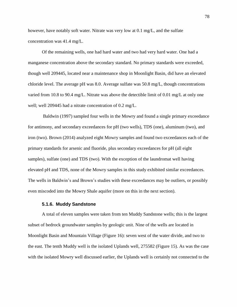
78
however, have notably soft water. Nitrate was very low at 0.1 mg/L, and the sulfate
concentration was 41.4 mg/L.
Of the remaining wells, one had hard water and two had very hard water. One had a
manganese concentration above the secondary standard. No primary standards were exceeded,
though well 209445, located near a maintenance shop in Moonlight Basin, did have an elevated
chloride level. The average pH was 8.0. Average sulfate was 50.8 mg/L, though concentrations
varied from 10.8 to 90.4 mg/L. Nitrate was above the detectible limit of 0.01 mg/L at only one
well; well 209445 had a nitrate concentration of 0.2 mg/L.
Baldwin (1997) sampled four wells in the Mowry and found a single primary exceedance
for antimony, and secondary exceedances for pH (two wells), TDS (one), aluminum (two), and
iron (two). Brown (2014) analyzed eight Mowry samples and found two exceedances each of the
primary standards for arsenic and fluoride, plus secondary exceedances for pH (all eight
samples), sulfate (one) and TDS (two). With the exception of the laundromat well having
elevated pH and TDS, none of the Mowry samples in this study exhibited similar exceedances.
The wells in Baldwin’s and Brown’s studies with these exceedances may be outliers, or possibly
even miscoded into the Mowry Shale aquifer (more on this in the next section).
5.1.6. Muddy Sandstone
A total of eleven samples were taken from ten Muddy Sandstone wells; this is the largest
subset of bedrock groundwater samples by geologic unit. Nine of the wells are located in
Moonlight Basin and Mountain Village (Figure 16): seven west of the water divide, and two to
the east. The tenth Muddy well is the isolated Uplands well, 275582 (Figure 15). As was the case
with the isolated Mowry well discussed earlier, the Uplands well is certainly not connected to the

79
other Muddy wells. Additionally, there is no lithology recorded with the well log; its coding into
the Muddy Sandstone is based on the surrounding surface geology.
The Muddy Sandstone samples average to be the most depleted with respect to
oxygen-18 (tied with the Kootenai Formation) and the third-most depleted with respect to
deuterium (Figure 20). The standard deviations for both isotopes in the Muddy are the smallest
along all of the bedrock units in the main study area, meaning they are more tightly grouped
around their median value than is the case in any other bedrock aquifer. Overall, all the water
isotope values from the Muddy wells are quite similar. The data points group on and between the
Butte and Global MWLs (Figure 28). The isolated Uplands well is the most depleted of the
Muddy wells with respect to deuterium, and one of the most depleted with respect to oxygen-18.
The two wells on the east side of the divide are among the most isotopically enriched, with the
wells on the west side ranging from the most enriched in the unit (well 215507) to nearly as
depleted as the Uplands well.
From the topography shown in Figure 16, the water pathways west of the divide are
complex. All the wells are at a high enough elevation that snow recharge should be a major
factor, so they all should be on the more depleted end of the spectrum. The presence of some
relatively enriched samples indicates overland evaporated recharge as well. The wells on the east
side are likely also getting that overland recharge. The Uplands well is by far the deepest of the
Muddy wells (880 feet) and is mostly likely receives deep groundwater recharge, plus snow.

80
Figure 28: Water Isotopes in Muddy Aquifer
Six wells in the Muddy Sandstone unit were sampled for carbon. Four of the six wells,
located in Moonlight Basin and adjacent Mountain Village, grouped tightly in terms of DIC, with
concentrations from 28.3 to 58.1 mg/L, and δ13C values from -13.0‰ to -13.8‰ (soil gas
source). One well – the Uplands well (275582), which is isolated from the other Muddy wells on
the opposite end of the study area, and is the deepest of the Muddy wells – had a very high DIC
concentration of 98.1 mg/L and a δ13C value of -11.6‰ (still a soil CO2 source). The final well,
259685, located in the far northwest reaches of Moonlight Basin, had a concentration of
59.2 mg/L and a δ13C value of -7.4‰, indicating carbonate rocks as the DIC source. There are no
carbonate rocks in the immediate area, and none noted in the well’s lithology log. Based on the

81
landslide map of the region complied by Vuke (2013), it is in or very near to a landslide deposit,
and the well log confirms layers of fractured rock above the well screen. Water percolation
through these fractured rock layers may account for the enriched δ13C in DIC signature
(Singleton and Moran, 2010), or it may be receiving seepage from the Kootenai Formation
below.
Five of the six wells had DOC concentrations above the detection limit, ranging from
0.39 to 1.74 mg/L. Three of the samples were right around the -22‰ δ13C value to pinpoint
marine sediments as the carbon source (-21.9‰ to -22.2‰); these include two high-elevation
wells in Moonlight Basin and the isolated Uplands well. The other two were much more depleted
with respect to carbon-13, with values of -27.0‰ and -31.8‰. These two wells had vascular
plant matter or microbial biomass as their DOC source. These wells are located quite a distance
from each other, but they are very similar in both DOC and DIC concentrations, and in δ13C
values for both types of carbon. They may represent a contiguous stretch of the Muddy
Sandstone.
Of the nine Muddy Sandstone wells tested for tritium, five showed modern water, two
showed a mix of pre- and post-bomb pulse waters, and two had tritium levels low enough to
mark them as old, pre-pulse waters (Table XVI). The five modern-aged wells, all on the
downslope side of the Lone and Fan Mountain area, are probably getting most of their recharge
from fresh snowmelt, like the nearby Frontier and dacite wells. One mixed water well, 259706, is
located on a possible landslide area. This well could be receiving a mix of older groundwater
from the base bedrock, and more recent recharge from closer to the surface. The Uplands well,
which has already been noted as isolated and disconnected from the other wells completed in the
Muddy, also has mixed water tritium values.

82
The two old water wells are a bit perplexing. One is 259685, the same well with δ13C in
DIC values indicating either a carbonate rock source or shallow recharge through the fractured
landslide deposit above the well screen. It is possible its location on the landslide deposit means
it is getting some old water recharge from the base bedrock. The other old well, the Lee’s Pool
well (230804), is in an area that should be receiving frequent fresh snowmelt recharge, and it is
relatively shallow compared to other wells in the formation, at 238 feet deep. However, the well
log for 230804 shows granite and clay layers that may be acting as confining layers, preventing
most precipitation-based recharge and limiting recharge to old bedrock water from below.
Brown (2014) could not determine a unique water type for the Muddy Sandstone. Of the
ten water quality samples from the unit collected for this study, sodium was the dominant cation
in seven samples, and the secondary cation in an eighth. There were two samples each with
sodium bicarbonate, sodium bicarbonate-carbonate, and sodium bicarbonate-sulfate; one was a
sodium-calcium bicarbonate-sulfate type, and one was a calcium-sodium-magnesium
bicarbonate type. The remaining two samples were of the calcium bicarbonate water type
(Table XX).
The Stiff diagrams for the Muddy Sandstone wells (Appendix G) show two main shapes:
one for the three calcium-dominant wells, and one for the seven where sodium is the most
abundant cation. Also notable is the variance in how mineralized the wells are. Wells 215507
and 230803, for example, do not have any major ions at a concentration greater than 2 meq/L,
while the Uplands well (275582) is highly mineralized with sodium alone at a concentration of
nearly 12 meq/L.

83
Table XX: Water Types in Muddy Aquifer
GWIC ID Water Type
230803 Ca-HCO3
215507 Ca-HCO3
230689 Ca-Na-Mg-HCO3
259357 Na-Ca-HCO3-SO4
231745 Na-HCO3
259685 Na-HCO3
244347 Na-HCO3-CO3
230804 Na-HCO3-CO3
259706 Na-HCO3-SO4
275582 Na-HCO3-SO4
Water quality is an issue with the wells in this geologic unit; two of the wells had a
primary exceedance, and an additional seven had at least one secondary standard exceedance
each. The primary exceedances were for arsenic (at nearly twice the EPA limit) at well 244347,
and fluoride (at nearly five times the EPA limit) at well 259685. Luckily, neither well is being
used for drinking water at this time; both are currently unused. Seven of the ten wells had a pH
value greater than 8.5, with an eight just under the limit at 8.4; the average pH was 8.9. All of the
wells with a sodium-dominant water type had a pH of 8.4 or greater. The Lee’s Pool well
(230804) a pH of 10.1, the highest pH recorded in this study. Three wells had above-limit
concentrations of manganese, and one was above the standard limit for TDS. One well had
moderately hard water, and eight had elevated sodium concentrations. Nitrate was very low, with
concentrations above detection limit in only two of the wells, with an average of 0.2 mg/L.
Sulfate averaged 23.9 mg/L in the Moonlight Basin/Mountain Village wells, but was 188.6 mg/L
in the isolated Uplands well. Field sulfide analyses were performed at six Muddy Sandstone
wells, all west of the divide, with results ranging from 0.00 (measured) to 0.22 mg/L.
84
In addition to poor drinking water quality, five wells exceed limits for use as irrigation
water, due to high SAR, high molybdenum concentrations, or both. The well with high fluoride
would also be unsuitable for livestock use.
Baldwin (1997) examined two Muddy wells, both exceeded the primary standard for
arsenic, and one for antimony; both wells also exceeded the secondary standard for pH, and there
was one exceedance each for TDS, aluminum, manganese, and iron. Brown (2014) found only
one occurrence of a secondary standard exceedance, for manganese, in four Muddy wells.
However, the results for the Mowry Shale in that study (as detailed in the previous section) are
similar to this study’s Muddy Sandstone results. There is a strong possibility that some of the
wells originally assigned to the Mowry aquifer are in fact completed in, or at least somehow
drawing their water from, the Muddy Sandstone.
5.1.7. Kootenai Formation
The five Kootenai Formation wells examined in this study are all located in Yellowstone
Club and the adjacent Spanish Peaks area (Figure 17). By average, the Kootenai wells are the
most isotopically depleted in the study area in both oxygen-18 (tied with the Muddy Sandstone)
and deuterium (Figure 20). However, upon examining the individual wells, one is considerably
more enriched than the other four (Figure 29). The most enriched well in the aquifer is 192865,
the Whiskey Barrel well in Yellowstone Club, and the elevation of the bottom of the well is
about 250 feet below the elevation of the South Fork of the West Fork of the Gallatin River in
this area. Therefore, the well is likely experiencing some surface water interaction, which would
account for the enrichment in water isotopes. This suggests groundwater/surface water
interaction in the region, which would not typically be expected in wells so deep.

85
Figure 29: Water Isotopes in Kootenai Aquifer
Three of the Kootenai wells were sampled for carbon analysis. They were not consistent
in their DIC concentrations, ranging from 27.0 to 73.5 mg/L. The Spanish Peaks PWS well
(239759), which had the lowest DIC concentration, had a δ13C value indicating soil gas as the
DIC source (-11.8‰), and the other two with higher DIC levels had carbonate rock δ13C values
(-9.1‰ and -7.0‰). Of the two Kootenai wells with detectable DOC, the Spanish Peaks PWS
well had just 0.07 mg/L DOC and a δ13C value of -32.2‰, indicating a definite plant source. The
other well, Eglise Road (192966, in Yellowstone Club) had 0.31 mg/L DOC and δ13C of -
22.6‰, for a plant/marine mix. This is the same well that had the highest DIC concentration of
the three. Indicators of both carbonate rocks and marine shales would be expected in this

86
geologic formation; the traits of the Spanish Peaks PWS well are curious. The well’s water is
actually combined with that of a second well for the water system, but that well has the exact
same units in its stratigraphic column (with some slight differences in layer thicknesses), and is
also completed in the Kootenai Formation. The only difference is that it is drilled about 80 feet
deeper. Some other water influence is a possible explanation; the overlying Muddy Sandstone
aquifer may be leaking into the Kootenai in the vicinity of these wells.
Three Kootenai wells were sampled for tritium, yielding results of two modern waters
and one mix of pre- and post-bomb pulse water (Table XVI). The modern water results are
somewhat surprising, as the Kootenai Formation is one of the oldest units that was sampled for
tritium. However, the locations of the wells give possible explanation for the water ages. The
Eglise Road well (192966) is in an area likely dominated by snowmelt recharge; in that
particular area, the Kootenai may not be receiving much deep groundwater recharge. The other
modern-aged well is at the Spanish Peaks horse corral (237292), and is in close proximity to the
South Fork Gallatin River. It is likely that like the isotopically enriched well within the
Yellowstone Club, the Kootenai is getting some surface recharge from the river.
Among the five Kootenai wells, four different but similar water types were exhibited:
calcium-magnesium bicarbonate at two wells, and calcium-magnesium bicarbonate-sulfate,
calcium-magnesium-sodium bicarbonate, and calcium-magnesium-sodium bicarbonate-sulfate at
one well each (Table XXI). Brown’s determined water type for this formation was calcium-
magnesium-bicarbonate or magnesium-calcium-bicarbonate. The Stiff diagrams for theses
samples (Appendix G) all show the same general shape, so despite the variations in ion
concentrations, the wells all have similar water. This is close correlation by unit in terms of water
type is second only to that of the samples from the alluvial aquifer.

87
Table XXI: Water Types in Kootenai Aquifer
GWIC ID Water Type
192856 Ca-Mg-HCO3
192865 Ca-Mg-HCO3
239759 Ca-Mg-HCO3-SO4
192966 Ca-Mg-Na-HCO3
237292 Ca-Mg-Na-HCO3-SO4
All five wells in the Kootenai aquifer had at least one undesirable trait in water quality;
all were secondary standard exceedances and hardness levels. One well had high iron and
manganese concentrations; one had elevated chloride and hard water; one had elevated sodium,
high manganese, and very hard water, and the last two had elevated sodium and very hard water.
None of these are health hazards, but definitely affect the aesthetics of the water. The average pH
value in the Kootenai wells was 7.5, in the middle of the acceptable range for drinking water.
Nitrate was low at 0.5 mg/L, and the average sulfate concentration was 40.8 mg/L. Two wells
were analyzed for sulfide in the field, with results of 0.00 (measured) mg/L at the Spanish Peaks
Horse Corral and 0.06 mg/L at the Eglise Road Well in Yellowstone Club.
In Baldwin (1997), the two Kootenai wells investigated both exceeded the primary limit
for arsenic, both exceeded the secondary limit for pH, and one had a manganese exceedance.
Brown (2014) found secondary exceedances for iron (five), manganese (four), pH (one), and
TDS (one) in eight total samples.
5.1.8. Morrison Formation
The six Morrison Formation wells, all located in Yellowstone Club and Spanish Peaks
(Figure 17), have the widest variance in water isotope concentrations of all the aquifers
(Figure 20). When examined closely, the wells are isotopically grouped in two sets of three
(Figure 30); one set makes up three of the most isotopically depleted wells in the study area, and
the other three are much closer to the alluvium wells in terms of isotopic signature. In fact, one

88
of the Morrison wells – 176327, the Yellowstone Club Entrance Gate well, which also happens
to be the deepest drilled well in the study area – is the most isotopically enriched groundwater
sample in the study area with respect to oxygen-18, and the second-most enriched in deuterium.
As the elevation of all the wells would indicate primarily snow recharge, these three wells must
be getting some surface water interaction to account for the enriched isotopes.
Figure 30: Water Isotopes in Morrison Aquifer
Closer inspection of the well’s depth to water, its elevation, and the elevation of the
South Fork of the West Fork Gallatin River in the area, indicates that the Morrison Formation, at
least in this particular area, is experiencing surface water interaction at the river. The well is at an
elevation of 7,660 feet above sea level, and it is 898 feet deep, putting the bottom of the well at

89
6,762 feet. The South Fork’s elevation is between 7,040 and 7,080 feet in this area. Therefore,
the bottom of the Entrance Gate well is below the river. This explains the isotopically enriched
water at such a great depth, in such an old geologic unit. The depths to water in the other two
isotopically enriched wells – 219966, the Spanish Peaks Entrance Gate, and 234783, the
Yellowstone Club Sewage Treatment Plant well – are also below the elevation of the river. The
Spanish Peak Entrance Gate well is further from the river than the other two, so overland flow
recharge may also play a role. The well is also located on the upturned, folded portion of the
Morrison Formation, which may enhance recharge to groundwater in the area.
Carbon suite analysis was performed on samples from two Morrison wells, both located
in Yellowstone Club. The two samples were very different as far as DIC concentrations – the
entrance gate well had 34.6 mg/L, while the Yellow Mule well (253676) had 130.6 mg/L. Both
had δ13C values indicating carbonate rocks as the DIC source (-9.5‰ and -6.3‰, respectively),
which makes sense as the Morrison Formation contains some freshwater limestone. While their
DOC concentrations were again quite different (1.02 mg/L and 2.80 mg/L), the δ13C values were
again in the same range, both signs of plant matter source for DOC (-25‰ and -23.9‰,
respectively). The Yellow Mule well had the highest DIC and DOC concentrations of all sixteen
carbon samples. Its δ13C in DOC value is right on the edge of the range for a mix of plant
matter/microbial biomass and marine sediment sources, which would make sense considering the
stratigraphy of the well column.
Three Morrison wells were sampled for tritium. The results were two modern waters and
one old, pre-bomb pulse water. The well with old water is the Yellow Mule well; with its depth
into the oldest geologic unit accessed in the region, visibly poor water quality, and terrible sulfur
odor, this is not unexpected.

90
The two modern results were somewhat surprising, as they were in the Kootenai
Formation directly above the Morrison. However, the wells are the entrance gate wells for both
Yellowstone Club and Spanish Peaks. As has already been discussed, they are both likely
experiencing surface water interaction and/or overland recharge.
Three of the Morrison Formation samples exhibited calcium-dominant water types: two
were calcium-magnesium bicarbonate, and one was calcium-magnesium-sodium bicarbonate-
sulfate. The other three were sodium-dominant: two were sodium bicarbonate, and one was
sodium bicarbonate-chloride (Table XXII). Brown (2014) did not have adequate sample numbers
in the formation to determine a unique chemical signature for the Morrison.
The Stiff diagrams for these wells varied quite a bit in shape (Appendix G). The Stiffs for
the two calcium-magnesium bicarbonate wells had the same shape, and the ones for the two
sodium bicarbonate wells did, also. The other two wells were considerable different than the
others. The Stiff diagram for the Yellow Mule well identified it as the most heavily mineralized
well in the study area.
Table XXII: Water Types in Morrison Aquifer
GWIC ID Water Type
176327 Ca-Mg-HCO3
234783 Ca-Mg-HCO3
176326 Ca-Mg-Na-HCO3-SO4
253676 Na-HCO3
262271 Na-HCO3
219966 Na-HCO3-Cl
There were water quality issues with all six Morrison wells. The Yellow Mule well was
the worst of all wells in the study area, with a pH of 9.2, a sodium concentration of 288.9 mg/L,
elevated fluoride of 2.6 mg/L, TDS of 692.0, and total sulfide of 23.15 mg/L. While technically
no EPA primary health standards are exceeded, the water is unusable for anything other than

91
flushing the toilet in the nearby gate station, and barely that: the hydrogen sulfide odor is so
strong that windows must be left open at all times, and headaches and nausea are common
among the security guards who take shifts there (personal communications, 2015).
Among the other wells, the Equine Center well (176326) had elevated sodium,
exceedances for manganese and sulfate, the highest TDS concentration in the study at
752.2 mg/L, and the hardest water in the study area at 470.6 mg/L. The American Spirit well
(262271) had a pH exceedance (8.63), elevated sodium, elevated fluoride, and elevated barium
(though still well below the EPA limit). The Spanish Peaks Entrance Gate well had just elevated
sodium, and the Yellowstone Club Entrance Gate and Sewage Treatment Plant wells just had
hard water.
Excepting the Yellow Mule well, the average pH was 7.9. Nitrate was low among the
Morrison wells at an average of 0.4 mg/L. Not including the American Spirit well, the average
sulfate concentration was 24.6 mg/L. Three of the six wells are unsuitable for irrigation use due
to high molybdenum and/or SAR, and two are unsuitable for stock water due to their fluoride
concentrations. Brown’s water quality study (2014) only examined two Morrison wells, and
found just one secondary standard exceedance each for pH and TDS.
5.1.9. Madison Group
Only one sample site in this study came from the Madison Group – a spring (255289) on
the far eastern edge of the study area (Figure 15). The spring site is isolated from the rest of the
study area, close to the Spanish Peaks Fault. It has been sampled for water isotopes four times,
and for water chemistry and quality twice. It was not sampled for either carbon or tritium.
The average of the Madison oxygen-18 and deuterium isotope values puts it in the middle
of all the other aquifers, slightly toward the depleted end of the range (Figure 20). The Madison

92
has the second-smallest standard deviation for oxygen-18 and the smallest for deuterium of all
the aquifers, meaning the data group tightly around the mean. Its average is most similar to that
of the Morrison Formation, which is also the geologic unit closest in age.
Water type analyses yielded a calcium-magnesium bicarbonate-sulfate type for both
samples; the Stiff diagrams for the two water quality samples are almost identical (Appendix G).
This matches the water type Brown (2014) determined for the Madison Group.
Both water quality samples were very hard, and one sample also exceeded the secondary
standard limit for manganese. Otherwise there were no water quality issues. Nitrate was low at
0.1 mg/L, sulfate averaged 108.5 mg/L, and the average pH was 7.8. Brown’s study (2014)
revealed no water quality issues in any of twelve Madison samples.
5.1.10. Summary of Findings by Aquifer/Geologic Unit
Sorting groundwater samples by aquifer/geologic unit gave mixed results in terms of
water isotopes, carbon, tritium, water type, and water quality. There were definite similarities
within the sample set of each unit, but also some differences. The results did provide some
means to fingerprint waters, particularly expanding on Brown (2014) by adding isotope analysis
to general water chemistry.
Overall, the alluvial aquifer was the most uniform in all the factors analyzed. It had a
distinct isotopic signature with respect to oxygen-18 and deuterium, all samples had essentially
the same water type, and the carbon and tritium results were consistent within the aquifer.
Only two aquifers had unique isotopic signatures with regard to oxygen-18 and
deuterium: the alluvium and the rock glacier (Figures 19 and 20). The single Frontier Formation
sample cannot rightfully be called a signature for the aquifer. The remaining aquifers show so

93
much overlap in their isotopic values that a clear, distinct isotopic signature cannot be
determined for each of them.
Not surprisingly, the most isotopically enriched aquifers are the alluvium and the rock
glacier; the alluvium has significant surface water interaction, and the rock glacier is recharged
almost entirely by overland snowmelt that has a chance to undergo evaporation (and therefore
become more enriched), and by rain. The dacite wells and springs are on the more isotopically
enriched end of the groundwater spectrum, as well, also largely recharged by slightly evaporated
snowmelt and rainfall.
On the depleted end of the spectrum are the Morrison, Muddy, and Kootenai wells. These
wells are all located at elevations where the majority of their recharge will be from depleted
snowmelt. The lack of an evaporation signature implies that the snowmelt infiltrates the ground
in situ instead of flowing overland, restricting opportunities for evaporation and the resulting
enrichment. The Mowry and Madison aquifer averages are in the middle of the aquifer averages,
overlapping with both the relatively enriched and depleted aquifers.
With only a handful of wells sampled for carbon in each aquifer, it is not possible to
assign each aquifer a distinct carbon signature. There is also not enough similarity among the
samples in each aquifer to draw definitive conclusions; differing DIC and DOC sources in the
same aquifer are common, regardless of carbon concentrations. The alluvium aquifer is the
exception, as the three samples show the clearest correlation: all with DIC from soil-zone CO2,
and DOC from a mix of plant matter/microbial biomass and marine sediments.
The variation in tritium age-dating results in the Muddy, Kootenai, and Morrison aquifers
shows that the age of a geologic unit is not necessarily a reflection of the age of the water within.

94
Depth to water is also not a connection, as the deepest well sampled had modern water, and one
of the shallowest of the bedrock wells had old water.
Water quality was overall the best in the alluvium and dacite units. The rock glacier
spring also had good water, but is not productive enough for drinking water use. All other units
had at least secondary exceedances. The Muddy Sandstone contained the two primary
exceedances in the study.
The similarities between the Muddy, Kootenai, and Morrison aquifers strongly suggest
there is some groundwater interaction between the units. The overlaps in isotope values and
water types, especially, indicate that the bedrock layers may be fractured enough that there is
mixing of water between units. Though the Muddy Sandstone wells sampled in this study are not
connected to the Kootenai and Morrison wells sampled, there were enough clues – such as
carbonate rock signatures in Muddy Sandstone wells – to indicate vertical mixing between the
units in all areas. This adds to the difficulty in assigning chemical signatures to each aquifer, and
also to determining the main source for water in a well.
A very important consideration in the fingerprinting of waters by unit is the watershed
divide between Moonlight Basin and Mountain Village. The wells on either side of the divide
will not be connected to each other, even if they are completed in the same geologic unit. The
isolated Uplands and Meadow Village laundromat wells are also not connected to the rest of the
wells in their respective units. These disconnections provide evidence that the geologic units are
not continuous across the area, which adds to the difficulty in assigning chemical signatures to
any single unit.

95
5.2. Analysis by Region
The data were sorted by region to reveal any similarities. The oxygen-18 and deuterium
data, by region, are plotted in Figure 31. Average isotope values and standard deviations were
calculated and plotted for each region (Table XXIII, and Figures 32 and 33).
Figure 31: Water Isotopes by Region
Table XXIII: Water Isotope Values by Region
Region Average δ18O (‰) Standard Deviation Average δD (‰) Standard Deviation
Moonlight Basin -19.4 0.5 -146.3 4.5
Mountain Village -19.4 0.4 -145.9 2.7
Meadow Village -18.8 0.6 -146.3 4.1
Spanish Peaks -19.8 0.5 -151.7 2.6
Yellowstone Club -19.8 0.9 -150.3 6.6
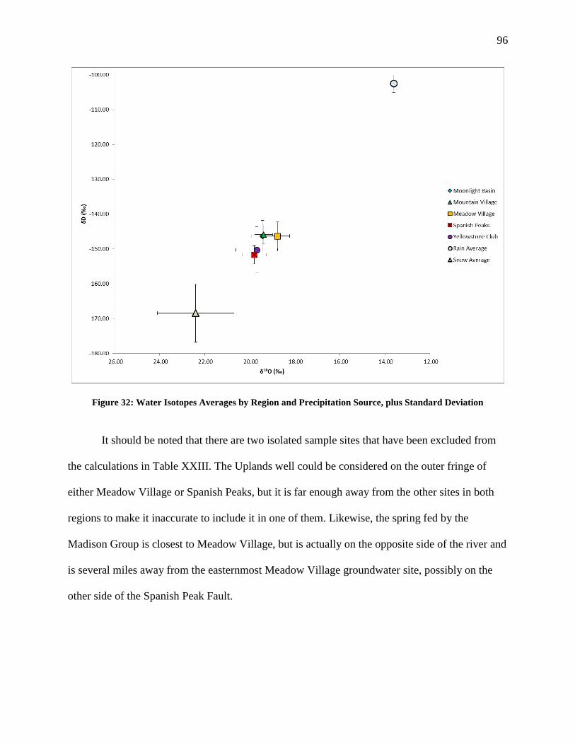
96
Figure 32: Water Isotopes Averages by Region and Precipitation Source, plus Standard Deviation
It should be noted that there are two isolated sample sites that have been excluded from
the calculations in Table XXIII. The Uplands well could be considered on the outer fringe of
either Meadow Village or Spanish Peaks, but it is far enough away from the other sites in both
regions to make it inaccurate to include it in one of them. Likewise, the spring fed by the
Madison Group is closest to Meadow Village, but is actually on the opposite side of the river and
is several miles away from the easternmost Meadow Village groundwater site, possibly on the
other side of the Spanish Peak Fault.

97
Figure 33: Water Isotope Averages by Region, plus Standard Deviation
Carbon suite values, by region, are shown in Tables XXIV and XXVI, and Figures 34-37,
using the same plotting schemes as were used by geologic unit. Tritium concentrations, by
region, are listed in Table XXVI.

98
Table XXIV: Carbon Results Sorted by Region
GWIC
ID Location Aquifer pH
DIC
(mg/L)
δ13C-DIC
(‰) DOC
mg/L
δ13C-DOC
(‰)
Total
DC
(mg/L)
275582 Isolated (Uplands) Muddy 8.4 98.1 -11.6 1.7 -21.9 99.8
281359 Meadow Village Alluvium 7.6 69.4 -13.0 0.5 -23.2 69.9
281363 Meadow Village Alluvium 7.7 54.2 -11.9 0.6 -23.4 54.8
281366 Meadow Village Alluvium 7.5 57.2 -12.5 1.4 -23.7 58.6
230689 Moonlight Basin Muddy 7.9 36.2 -13.0 0.4 -22.0 36.6
259357 Moonlight Basin Muddy 9.2 32.3 -13.1 0.4 -27.0 32.7
259685 Moonlight Basin Muddy 9.5 59.2 -7.4 BDL BDL 59.2
259706 Moonlight Basin Muddy 8.8 58.1 -13.5 0.6 -22.2 58.7
103496 Mountain Village Dacite 9.5 21.9 -14.5 0.3 -34.3 22.2
205931 Mountain Village Dacite 8.0 56.2 -6.9 0.2 -38.6 56.4
244347 Mountain Village Muddy 9.5 28.3 -13.8 0.5 -31.8 28.8
237292 Spanish Peaks Kootenai 7.7 53.9 -7.0 BDL BDL 53.9
239759 Spanish Peaks Kootenai 7.6 27.0 -11.8 0.1 -32.2 27.1
176327 Yellowstone Club Morrison 7.7 34.6 -9.5 2.8 -23.9 37.4
192966 Yellowstone Club Kootenai 7.5 73.5 -9.1 0.3 -22.6 73.8
253676 Yellowstone Club Morrison 9.2 130.6 -6.3 1.0 -25.0 131.6
Table XXV: Carbon Averages and Standard Deviations, by Region
Region DIC
(mg/L)
δ13C-DIC
(‰) DOC
(mg/L)
δ13C-DOC
(‰)
Moonlight Basin Mean 46.4 -11.8 0.5 -23.7
Std Dev 12.3 2.5 0.1 2.3
Mountain Village Mean 35.5 -11.7 0.3 -34.9
Std Dev 14.9 3.4 0.1 2.8
Meadow Village Mean 60.3 -12.4 0.8 -23.4
Std Dev 6.6 0.5 0.4 0.2
Spanish Peaks Mean 40.4 -9.4 0.1 -32.2
Std Dev 13.4 2.4 0.0 0.0
Yellowstone Club Mean 79.6 -8.3 1.4 -23.8
Std Dev 39.4 1.4 1.0 1.0
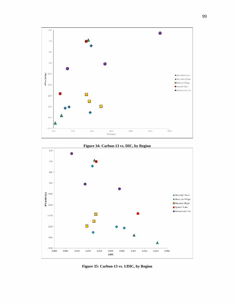
99
Figure 34: Carbon-13 vs. DIC, by Region
Figure 35: Carbon-13 vs. 1/DIC, by Region
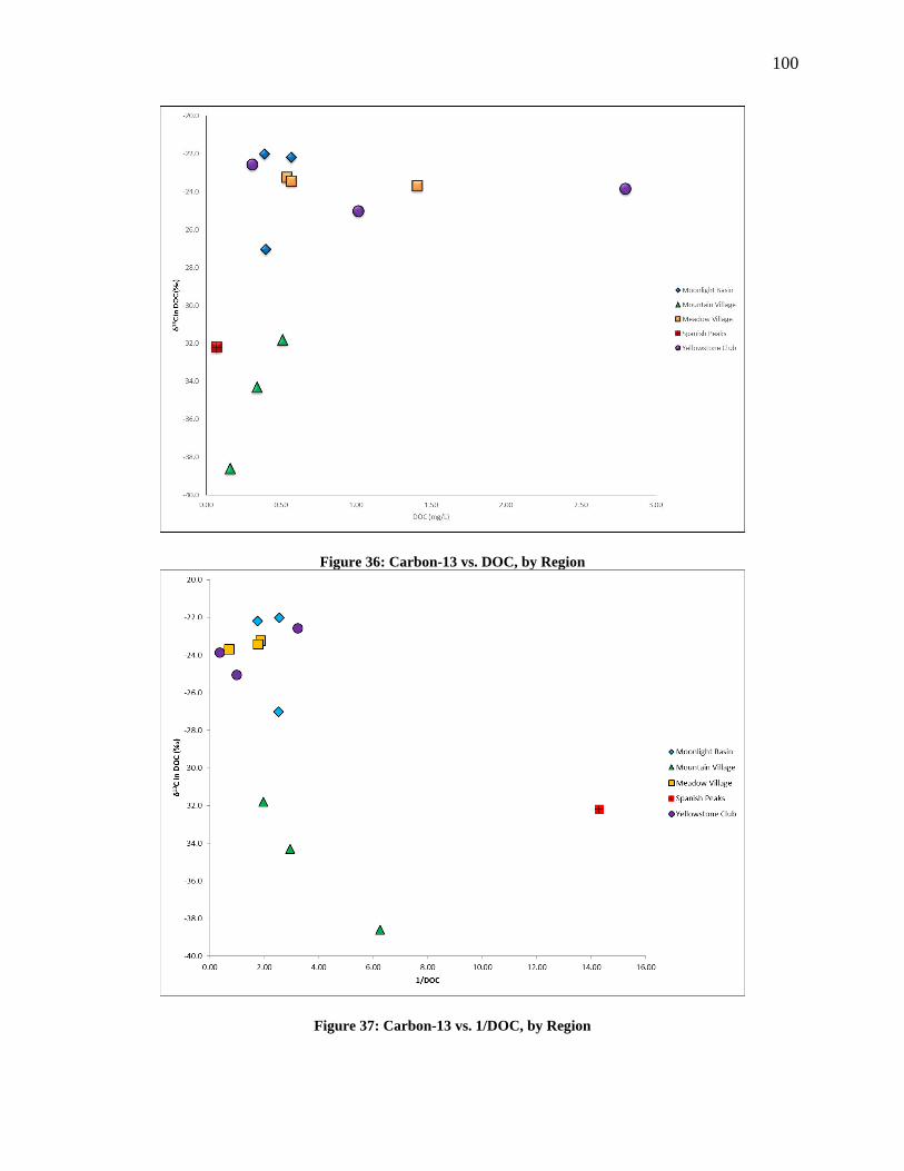
100
Figure 36: Carbon-13 vs. DOC, by Region
Figure 37: Carbon-13 vs. 1/DOC, by Region

101
Table XXVI: Tritium Concentrations, by Region
GWICID Area Aquifer Tritium (TU) Age Category
275582 Isolated Muddy 2.5 Mix
281363 Meadow Village Alluvium 6.2 Modern
281371 Meadow Village Alluvium 5.6 Modern
215507 Moonlight Basin Muddy 6.4 Modern
230689 Moonlight Basin Muddy 6.3 Modern
230804 Moonlight Basin Muddy <0.8 Old
259357 Moonlight Basin Muddy 4.1 Mix/Modern
259685 Moonlight Basin Muddy <0.8 Old
259706 Moonlight Basin Muddy 0.9 Mix
279062 Moonlight Basin Frontier 6.4 Modern
279080 Moonlight Basin Dacite 7.3 Modern
103496 Mountain Village Dacite 4.2 Mix/Modern
205931 Mountain Village Dacite 6.1 Modern
230803 Mountain Village Muddy 7.3 Modern
244347 Mountain Village Muddy 6.5 Modern
219966 Spanish Peaks Morrison 4.3 Mix/Modern
237292 Spanish Peaks Kootenai 5.0 Modern
239759 Spanish Peaks Kootenai 2.0 Mix
176327 Yellowstone Club Morrison 6.7 Modern
192966 Yellowstone Club Kootenai 5.1 Modern
253676 Yellowstone Club Morrison <0.8 Old
5.2.1. Moonlight Basin
The Moonlight Basin region covers the most land area of the five regions, and has the
most isotope samples. There are also four different geologic units represented in the region:
Frontier, Dacite, Mowry, and Muddy. For the purpose of calculations and comparisons, only the
sites west of the watershed divide (Figure 16) are considered in Moonlight Basin, regardless of
well name or property ownership. Those east of the divide are considered part of Mountain
Village.
The samples cover one of the narrowest ranges of oxygen-18 values of all the regions,
and the second-widest range of deuterium values (Table XXII). There is a small cluster of three

102
samples that are slightly more depleted than the rest (Figure 38) – wells 230804, 231745, and
259685 (Figure 16). All three of the more depleted wells are in the same geologic unit, the
Muddy Sandstone, but that is where their similarities end. They are not geographically close to
each other, have all different depths, and do not appear to be on the same flowpath based on
geology/topography. As was discussed in detail in the section on the Muddy Sandstone, while all
these sites should be recharged primarily by depleted snowmelt and deep groundwater, the other
wells and springs that are slightly more enriched may be getting some overland recharge as well.
Figure 38: Water Isotope Values in Moonlight Basin

103
Four of the wells sampled for carbon were located in Moonlight Basin. Their DIC
concentrations ranged from 32.3 to 59.2 mg/L (average 46.4 mg/L). Three of them had nearly
identical δ13C in DIC values, tightly grouped from -13.5‰ to -13‰, in the range for a soil gas
source of carbon. The fourth well, 259685, had a δ13C value of -7.4‰. As discussed in the
Muddy Sandstone section, this low value is an indicator of carbonate rocks as the carbon source
(possible seepage from limestone-bearing units below) or recharge from meltwater that traveled
overland before percolating down. This well did not have DOC concentration above the
detection limit. The other three wells had concentrations ranging from 0.4 to 0.6 mg/L. One had
δ13C in DOC values typical of a marine sediment source, one for plant matter/microbial biomass,
and one for a mix.
Nine tritium samples were collected in Moonlight Basin, the most of any region. Of
them, six wells had modern water, one had a mix of pre- and post-bomb pulse water, and two
had old, pre-pulse water, according to the 1997 Clark and Fritz scale (Table XXVI). The details
on the individual wells can be found in the sections on their respective geologic units. Of note
here is that the region does not have a uniform water age.
Thirteen samples in Moonlight Basin were tested for water quality and water type. Nine
different chemical signatures were found. Overall, calcium bicarbonate type waters make up
eight of the samples: one calcium bicarbonate, two calcium bicarbonate-sulfate, one calcium-
magnesium bicarbonate-chloride, three calcium-magnesium bicarbonate-sulfate, and one
calcium-sodium-magnesium bicarbonate. The five sodium bicarbonate samples include one
sodium-calcium bicarbonate-sulfate, two sodium bicarbonate, one sodium bicarbonate-carbonate,
and one sodium bicarbonate-sulfate (Table XXVII). While there is no unifying water type for the
region, the individual Stiff diagrams (Appendix G) do show some smaller sub-regional trends.

104
Muddy Sandstone well 215507, dacite well 279080 and spring 279079, and Frontier well 279062
have nearly identical Stiff diagrams. These four sites are all grouped together on the northern
flank of Lone Peak. The Stiff diagrams for the remainder of the Muddy wells (excluding 230689)
have similar shapes as well. The two Mowry wells in the western part of the basin are similar, as
are 230689 and 209445 on the eastern side. So there are some sub-regional pockets of similar
waters.
Table XXVII: Water Types in Moonlight Basin
GWIC ID Water Type
215507 Ca-HCO3
279062 Ca-HCO3-SO4
279080 Ca-HCO3-SO4
209445 Ca-Mg-HCO3-Cl
215510 Ca-Mg-HCO3-SO4
231031 Ca-Mg-HCO3-SO4
279079 Ca-Mg-HCO3-SO4
230689 Ca-Na-Mg-HCO3
259357 Na-Ca-HCO3-SO4
231745 Na-HCO3
259685 Na-HCO3
230804 Na-HCO3-CO3
259706 Na-HCO3-SO4
There were water quality issues with ten of the wells in the basin. The primary standard,
fluoride, was exceeded by nearly five times the acceptable limit at well 259685; as discussed
earlier, this well is luckily not in use. Secondary standard exceedances were pH at six wells (the
average pH for the region was 8.6) and manganese at four wells. Six wells had elevated sodium
levels, one had elevated chloride, two had hard water, and two had very hard water. Nitrate was
low, with an average for the six samples with detectible levels of 0.3 mg/L. Sulfate
concentrations varied, with an average of 32.7 mg/L. Seven wells were tested in the field for
sulfide, with an average concentration of 0.09 mg/L. In addition to the drinking water issues,

105
three wells were unusable for irrigation due to SAR or molybdenum levels, and the high fluoride
well was unsuitable for use as stock water.
Based on topography and the presence of the water divide, the water table in Moonlight
Basin slopes down and west toward Jack Creek. It does not end up in the West Fork drainage.
5.2.2. Mountain Village
There are seven isotope samples from five sites (four wells and one spring) in the
Mountain Village area, and they are tightly grouped along the GMWL (Figure 39). Two wells
are in a dacite sill, two are in the Muddy Sandstone, and the spring originates in the rock glacier.
As shown in Table XXIII, the Mountain Village area is the second most enriched with respect to
oxygen-18 and the most enriched with respect to deuterium, with tight standard deviations.
Figure 39: Water Isotope Values in Mountain Village

106
As discussed in the individual geologic units sections, the fractured natures of these units, along
with overland flow, can account for the relative enrichment of these isotopes for the high
elevation. There is a great deal of overlap with the Moonlight Basin range of values (Figure 33),
but it is important to remember that the regions are adjacent but not connected, due to the
watershed divide (Figure 16).
Three wells were sampled for carbon in Mountain Village: two dacite wells (103496 and
205931), and a third well completed in the Muddy Sandstone (244347). DIC concentrations
ranged from 21.9 mg/L to 56.2 mg/L, with an average of 35.5 mg/L. Two had δ13C in DIC values
indicating a soil CO2 carbon source, while the third had a value indicating a carbonate rock
source (from overland flow or seepage from an underlying limestone-bearing unit).
Concentrations of DOC ranged from 0.16 mg/L to 0.51 mg/L, and all three had δ13C in DOC
values that corresponded with a vascular plant matter or microbial biomass source.
The wells sampled for carbon were also sampled for tritium, plus well 230803. All four
had concentrations indicative of modern-aged water by the Clark and Fritz scale (1997).
Three different water types were found among the five water quality samples. One of the
Muddy wells and the rock glacier spring both had a calcium bicarbonate water type. One of the
dacite wells had a calcium-sodium bicarbonate water type, and the remaining dacite well and
Muddy well had sodium bicarbonate-carbonate water (Table XXVIII). The Stiff diagrams
(Appendix G) did not show anything that would not be expected: the wells with the same water
type had similar diagrams. The sites with similar types were also physically close to each other
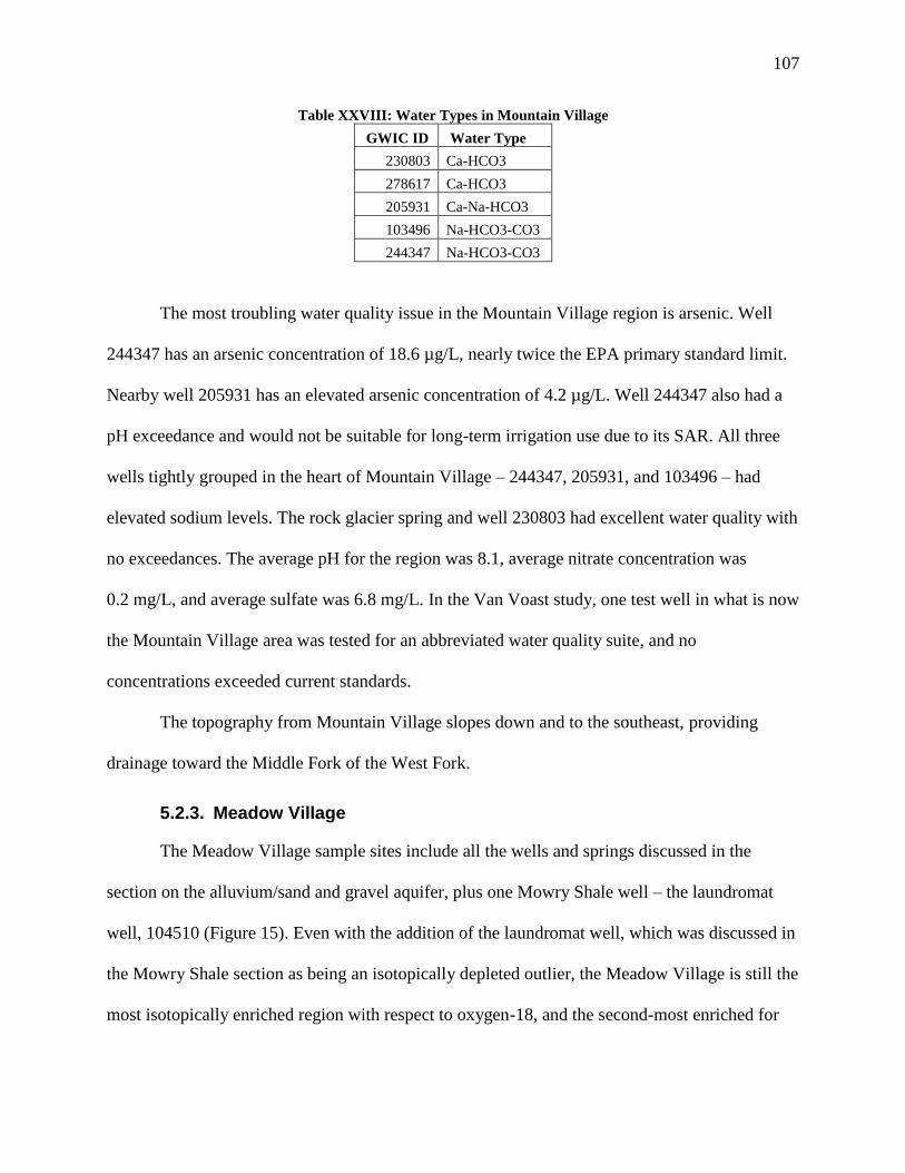
107
Table XXVIII: Water Types in Mountain Village
GWIC ID Water Type
230803 Ca-HCO3
278617 Ca-HCO3
205931 Ca-Na-HCO3
103496 Na-HCO3-CO3
244347 Na-HCO3-CO3
The most troubling water quality issue in the Mountain Village region is arsenic. Well
244347 has an arsenic concentration of 18.6 µg/L, nearly twice the EPA primary standard limit.
Nearby well 205931 has an elevated arsenic concentration of 4.2 µg/L. Well 244347 also had a
pH exceedance and would not be suitable for long-term irrigation use due to its SAR. All three
wells tightly grouped in the heart of Mountain Village – 244347, 205931, and 103496 – had
elevated sodium levels. The rock glacier spring and well 230803 had excellent water quality with
no exceedances. The average pH for the region was 8.1, average nitrate concentration was
0.2 mg/L, and average sulfate was 6.8 mg/L. In the Van Voast study, one test well in what is now
the Mountain Village area was tested for an abbreviated water quality suite, and no
concentrations exceeded current standards.
The topography from Mountain Village slopes down and to the southeast, providing
drainage toward the Middle Fork of the West Fork.
5.2.3. Meadow Village
The Meadow Village sample sites include all the wells and springs discussed in the
section on the alluvium/sand and gravel aquifer, plus one Mowry Shale well – the laundromat
well, 104510 (Figure 15). Even with the addition of the laundromat well, which was discussed in
the Mowry Shale section as being an isotopically depleted outlier, the Meadow Village is still the
most isotopically enriched region with respect to oxygen-18, and the second-most enriched for

108
deuterium (Figure 33 and Table XXIII). As shown in Figure 40, the laundromat well is
significantly depleted compared to the alluvial sites in the region.
Figure 40: Water Isotope Values in Meadow Village. The isolated data point belongs to well 104510.
The two tritium-sampled wells in the Meadow Village, as discussed in the section on the
alluvial aquifer, both had modern-aged water (Table XXVI). This would be expected for an
alluvial aquifer with surface water interaction.
The water type of calcium-magnesium bicarbonate dominates the Meadow Village,
accounting for eleven of the samples (two of them with elevated chloride, as shown in
Table XXIX). One spring sample was calcium-magnesium-sodium bicarbonate-chloride type,
and the laundromat well is the sodium-bicarbonate type. This is the outstanding sample that does

109
not match the others in the Mowry Shale at all, so it is an outlier by both aquifer and by region.
An examination of the Stiff diagrams (Appendix G) reveals that the laundromat well does not
look at all like the alluvial wells. It does look somewhat similar to the Uplands well to the south
(Figure 15), but the two wells are unlikely to be connected. This could serve as an indication that
the Uplands well is actually in the Mowry Shale, and not in the Muddy Sandstone, as previously
thought.
Table XXIX: Water Types in Meadow Village
GWIC ID Water Type
281360 Ca-Mg-HCO3
281362 Ca-Mg-HCO3
281363 Ca-Mg-HCO3
281366 Ca-Mg-HCO3
281367 Ca-Mg-HCO3
281368 Ca-Mg-HCO3
281371 Ca-Mg-HCO3
281372 Ca-Mg-HCO3
281373 Ca-Mg-HCO3
278297 Ca-Mg-HCO3-Cl
281359 Ca-Mg-HCO3-Cl
280689 Ca-Mg-Na-HCO3-Cl
104510 Na-HCO3
Water quality of the alluvial wells and springs was discussed earlier in the alluvial aquifer
section. The laundromat well was again an outlier, with extremely soft water (compared to the
hard water of the alluvium), a pH exceedance, elevated sodium, and an SAR too high for
irrigation use.
Twenty domestic and business wells, four test wells, and four springs were tested for
various water quality parameters in Van Voast’s 1972 study in the Meadow Village area and
extending southward along the main Gallatin River. The only exceedances noted at that time
were two wells and one spring with TDS concentrations greater than 500 mg/L, and one of those

110
wells also had a pH exceedance. Six wells had elevated sodium levels, but none above the WHO
objective limit of 200 mg/L.
Most of the water from the Meadow Village drains eastward directly toward the West
Fork Gallatin River. Along the southern edge of the region (Figure 15), drainage is into the South
Fork, which then drains into the main West Fork.
5.2.4. Spanish Peaks
The Spanish Peaks wells are, on average, the most depleted in the study area for both
oxygen-18 (tied with Yellowstone Club) and deuterium (Table XXIII). The three samples from
the Spanish Peaks area are the second-most tightly grouped of all the regions (Figures 33 and
41). Two of the wells are completed in the Kootenai Formation (237292 and 239759), with the
Figure 41: Water Isotope Values in Spanish Peaks

111
third in the Morrison (219966). The Spanish Peaks area is roughly the same size as Meadow
Village, so the wells are in close proximity to each other (Figure 17).
Two Spanish Peaks wells were tested for carbon. Well 237292, the entrance gate well,
had 53.9 mg/L DIC (carbonate rock source) and non-detectable DOC. Well 239759, PWS #3,
had just 27.0 mg/L DIC from soil CO2, and 0.07 mg/L DOC from plant matter/microbial biomass
sources. Both wells are in the limestone-bearing Kootenai Formation, but the screening in well
239759 is below a limestone layer (GWIC, 2016), so the water may not be picking up the typical
carbonate rock δ13C signature.
All three wells in Spanish Peaks were tested for tritium. Two wells, 219966 and 237292,
had modern water, and 239759 had a mix of pre- and post-pulse water (Table XXVI).
Each well in Spanish Peaks had a different water type: calcium-magnesium bicarbonate-
sulfate, calcium-magnesium-sodium bicarbonate sulfate, and sodium bicarbonate chloride
(Table XXX). The two Kootenai wells actually have very similar Stiff diagrams (Appendix G),
as sodium is a tertiary cation in well 237292. The Stiff diagram for well 219966 is very different.
Table XXX: Water Types in Spanish Peaks
GWIC ID Water Type
239759 Ca-Mg-HCO3-SO4
237292 Ca-Mg-Na-HCO3-SO4
219966 Na-HCO3-Cl
Water quality for the region was good overall. The average pH was 7.7, average nitrate
was 0.4 mg/L, and average sulfate was 57.0 mg/L. All three wells in Spanish Peaks had elevated
sodium concentrations, with well 219966 just below the WHO recommended limit of 200 mg/L.
As a result of its high sodium content, this well has very soft water, but would be unsuitable for
irrigation use due to its SAR. It also had a drinking water exceedance for TDS, and an irrigation
exceedance for molybdenum. The other two wells had very hard water, but no other water

112
quality issues. The horse corral well (237292) was tested for sulfide but the resulting
concentration was below the detection limit.
Drainage from Spanish Peaks follows topography down and southeast, toward the South
Fork of the West Fork Gallatin River.
5.2.5. Yellowstone Club
The set of eight Yellowstone Club isotope samples are the most depleted in oxygen-18
(tied with Spanish Peaks) and second-most depleted in deuterium (Table XXIII), and have the
largest standard deviations by far (Figure 33). All the wells are completed in the Kootenai and
Morrison formations, and are spread out over an area nearly as large as the Moonlight Basin
(Figure 17). The isotope data are plotted in Figure 42. The clustered data points do not represent
Figure 42: Water Isotope Values in Yellowstone Club

113
sites that are physically close to one another, as isotope values in the Yellowstone Club samples
are more dependent on recharge and surface water interaction than location (see the Kootenai
and Morrison Formation discussion sections for details).
Three Yellowstone Club wells were sampled for carbon: the much-discussed Yellow
Mule well (253676), the Eglise Road well (192966), and the entrance gate well (176327). The
sampled wells have a wide range of concentrations for both DIC (34.6 to 130.6 mg/L) and DOC
(0.31 to 2.80 mg/L). They are all in agreement on carbonate rocks as a DIC source; which is not
surprising as they are all screened in limestone-bearing geologic units. In terms of DOC sources,
176327 and192966 have plant matter/microbial biomass δ13C levels, and 253676 has a mix of
plant matter/microbial biomass and marine sediment sources.
The same three wells tested for carbon were also tested for tritium. The Yellow Mule
well had old, pre-pulse water, while the other two yielded modern water (Table XXVI).
Of the eight samples in Yellowstone Club, half of them have the exact same water type:
calcium-magnesium bicarbonate. One is calcium-magnesium-sodium bicarbonate, and another is
calcium-magnesium-sodium bicarbonate-sulfate. The remaining two wells have the sodium
bicarbonate chemical signature (Table XXXI). The Stiff diagrams (Appendix G) show most of
the calcium-dominant wells having nearly identical Stiff shapes, Kootenai and Morrison
Formation wells alike. Well 176326 is an outlier due to its higher sulfate presence. The two
sodium-dominant wells also have similar Stiff diagrams.
Water quality is a definite issue in the Yellowstone Club area. The Yellow Mule well’s
terrible water quality was thoroughly discussed in the section on the Morrison Formation, and it
had the worst water in Yellowstone Club as well. The average pH is 7.9 (with secondary
standard exceedances at the American Spirit well, 262271, and the Yellow Mule well), and

114
Table XXXI: Water Types in Yellowstone Club
GWIC ID Water Type
192856 Ca-Mg-HCO3
176327 Ca-Mg-HCO3
192865 Ca-Mg-HCO3
234783 Ca-Mg-HCO3
192966 Ca-Mg-Na-HCO3
176326 Ca-Mg-Na-HCO3-SO4
253676 Na-HCO3
262271 Na-HCO3
average nitrate was 0.4 mg/L. The Equine Center well (176326) had an exceedance for sulfate at
267.8 mg/L; otherwise the average concentration for the region was only 21.9 mg/L. Other
secondary exceedances included iron and manganese at well 192856 (Andesite Ridge),
manganese at Equine Center and Eglise Road wells, and TDS at the Equine Center and Yellow
Mule wells. Four wells have elevated sodium levels (the Yellow Mule well is over the WHO
objective of 200 mg/L), and three have elevated chloride. Three wells have hard water, and two
have very hard water. Two wells in the region were tested for sulfide in the field; the Eglise
Road well had a concentration of 0.06 mg/L and the Yellow Mule well had a concentration of
23.15 mg/L. Two wells are unsuitable for irrigation use: the American Spirit well due to very
high molybdenum, and the Yellow Mule well due to high SAR. The American Spirit and Yellow
Mule wells are also unsuitable for livestock use due to high fluoride concentrations.
As the topography shown in Figure 17 indicates, water flows from both north and south
in the region toward the South Fork.
5.2.6. Summary of Findings by Region
As can be seen in Figures 32 and 33, the region closest to having a unique isotopic
signature is the Meadow Village, which has the least overlap of its standard deviations with other
regions. Moonlight Basin and Mountain Village are so close in their averages that it would seem

115
certain that there is mixing between the two adjacent regions, but the presence of the watershed
divide makes mixing not possible. The two regions simply are so similar in their location and
precipitation recharge that they have similar signatures. Spanish Peaks and Yellowstone Club
also have close, overlapping isotopic signatures. In this case, mixing between the adjacent
regions is likely, as they share geologic units and the terrain is continuous between them. .
With the exception of the Meadow Village, it is difficult to assign a specific carbon
signature by region with so few samples in each area, just as it was when the samples were
divided by aquifer. The carbon results are more a factor of each individual well’s location and
lithology than its regional location.
In both Meadow Village and Mountain Village, all wells tested for tritium yielded
modern-aged waters. In the other three regions, water ages varied. When each well is examined
individually, it becomes clearer why it dates to a certain time period, but a general age category
cannot be assigned to either Moonlight Basin, Spanish Peaks, or Yellowstone Club.
The Meadow Village, having almost exclusively alluvial wells, had a dominant water
type signature of calcium-magnesium bicarbonate. In each other region, water types were a mix
of calcium and sodium types. There were smaller, sub-regional groupings of groundwater
sources with similar water types, there is too much variation to determine a unique chemical
signature for each region as a whole. There did appear to be mixing between Yellowstone Club
and Spanish Peaks, as similar water types were found in both regions, from two different units.
Drinking water quality was overall the best in Meadow Village (with the exception of the
laundromat well). Each other region had a mix of good quality and poor quality water, from both
health and aesthetic standpoints.

116
5.3. Connections and Mixing between Aquifers and Regions
At first glance, neither the investigation by aquifer nor by region seemed to reveal clear
signatures that could be used to define the water in each aquifer or region. This was not entirely
unexpected, as the subsurface geology has already been shown to be very complex. However, the
analysis does not stop here. There is more to the groundwater story in Big Sky.
There are several occurrences of similarities in water chemistry between wells that seem
unconnected, as they are in different aquifers. It has already been shown that just because wells
share an aquifer, does not mean they share the same water chemistry; being in the same region
doesn’t automatically link wells, either. Yet there are wells that seem to have similar waters, so
perhaps the connections are not just about aquifer or region, and are on a smaller scale.
Beginning with taking a closer look at the Piper diagrams that were originally presented
in Figures 12 and 13, it is immediately clear that all of the samples – groundwater and surface
water alike – fall into the lower left half of the center rhombus (left of the thick blue line in
Figure 43). This indicates that all of the water samples share the trait of weak acidic anions
exceeding strong acidic anions (Piper, 1944, and Chadha, 1999). Further, all of the surface water
samples and a majority of the groundwater samples, despite what tertiary cations and secondary
and tertiary anions they may have, are in the calcium-magnesium bicarbonate hydrofacies (left of
the thick red line in Figure 43). Piper (1944) described this water type as having carbonate
hardness, while Chadha (1999) described it as temporary hardness, but both refer to the same
thing: the water’s chemical properties are dominated by alkaline earth metals and weak acidic
anions. The remaining groundwater samples are in the sodium bicarbonate facies, dominated by
alkali metals and weak acidic anions (right of the thick red line in Figure 43). These waters are
extremely soft; they can cause problems in drinking/domestic use due to foaming, and in
irrigation due to deposits (Chadha, 1999).

117
Figure 43: Piper Diagrams for Groundwater and Surface Water, with Hydrofacies
The fact that all the samples are confined to these two quadrants, regardless of region and
aquifer, indicates there is some sort of interaction occurring between the waters both horizontally
(by area/region) and vertically (by aquifer). There is also strong evidence of groundwater and
surface water interaction (again, in multiple regions and aquifers) due to all of the surface water
samples and most of the groundwater samples being in the same quadrant. Further, based on the
separation between the samples in the calcium-magnesium bicarbonate and sodium bicarbonate
samples, it would seem that there is not much mixing between those two general water types.
Dividing the sample results according to water type revealed some patterns in isotope
concentrations. Averages and standard deviations were calculated for each water type that
occurred three or more times (Table XXXII). The calcium-dominant waters were more
isotopically enriched than the sodium-dominant waters. From the earlier discussions, sodium-
dominant waters tended to be in the higher elevations (more snow recharge) and in localized
areas where deep groundwater recharge was also likely, so this makes sense. Likewise, the
calcium-dominant waters were in areas with more rain recharge and surface-water interaction.

118
Table XXXII: Water Isotope Averages and Standard Deviations, by Water Type
Water Type Average δ18O (‰) Standard Deviation Average δD (‰) Standard Deviation
Ca-HCO3 -19.2 0.2 -143.0 1.4
Ca-Mg-HCO3 -18.8 0.5 -145.9 4.0
Ca-Mg-HCO3-Cl -18.5 0.6 -144.0 2.5
Ca-Mg-HCO3-SO4 -19.5 0.7 -147.0 4.6
Na-HCO3 -20.5 0.2 -155.0 2.2
Na-HCO3-CO3 -20.0 0.5 -150.7 3.7
A closer examination of δ13C vs. 1/DIC, sorted by both aquifer (Figure 44) and region
(Figure 45), shows possible mixing. When an element such as carbon is present at different
dissolved concentrations and isotopic abundances in two waters, a linear relationship between
the isotopic abundance and the inverse of concentration will be present if mixing is occurring
(Genereux et al., 2009).
Figure 44: δ13C vs. 1/DIC, by aquifer, with possible mixing lines in dashed black.

119
As seen in Figure 44, there is a lower line along which the alluvial wells, most of the
Muddy wells, and one of the dacite wells fall, and an upper line for the Kootenai, Morrison, and
outliers from the Muddy (well 259685) and dacite (well 205931) units. The wells along the upper
line are either from carbonate-bearing units (the Kootenai and Morrison formations), which tend
to be isotopically heavier, or from wells that have already been thought to be receiving seepage
from those underlying units. As the Morrison Formation is directly below the Kootenai
Formation in most of the study area, it would make sense to see these two units on a mixing line.
The lower line makes less sense, as the alluvial aquifer is disconnected from the Muddy
Sandstone.
These possible mixing lines are more significant on the plot sorted by region (Figure 45).
The upper line would imply mixing between the Spanish Peaks and Yellowstone Club wells,
with an outlier from each Moonlight Basin (well 259685) and Mountain Village (well 205931).
Not only does this make sense based on the geologic unit connections seen on Figure 44, but also
from the similarities in water isotopes and water types between Yellowstone Club and Spanish
Peaks discussed earlier. The outliers are not connected geographically, but geologically.
The lower line connects the Meadow Village wells with most of the Moonlight Basin and
Mountain Village wells. It has already been established that the Moonlight Basin and Mountain
Village are separated by the watershed divide, so there is not mixing between those units. It is
possible that there is mixing between the Mountain Village and Meadow Village.
The isolated Uplands well is not shown in Figure 45, but it can be seen on Figure 44 on
the lower mixing line. This would indicate that the well is more similar to the Meadow Village
wells to its north than the Spanish Peaks wells to its west.

120
Figure 45: δ13C vs. 1/DIC, by region, with possible mixing lines in dashed black.
These findings would imply three distinct large-scale flowpaths, matching what is
suggested by the topography of the study area. One on the west side of the watershed divide,
from the dividing ridgeline down to Jack Creek. The second begins on the east side of the
dividing ridge, through Mountain Village, extending down to Meadow Village. The third
straddles the South Fork of the West Fork Gallatin River, connecting the Yellowstone Club and
Spanish Peak areas. An in-depth examination of the water table and hydraulic gradient is beyond
the scope of this report, but a cursory look at the water level elevations collected for the larger
groundwater assessment (MBMG, in prep) indicated groundwater flowpaths similar to these
findings.

121
Another useful tool for seeing patterns of mixing is a plot of either δ18O or δD vs. SC.
A plot of δD vs. SC is shown in Figure 46 (δ18O vs. SC, though not presented here, yielded the
same pattern). The groundwater samples were separated by alluvium or bedrock origin.
Additionally, points were plotted for the average values of alluvium groundwater, bedrock
groundwater, surface water, rain, and snow samples. There was only one sample of each rain and
snow that had SC results. The rain and snow average points represent the average δD value of all
respective samples, graphed against the lone SC result for each.
Figure 46: Deuterium vs. SC. Triangles represent possible mixing.
To find evidence of mixing on such a plot, one looks for end points to a triangle;
everything within that triangle would be a mix of the three points. In this case, two triangles are

122
visible. The first, sketched in bright purple, indicates that all the surface data (except for one
outlying point – the sewage effluent sample, 246755) is a mix of rain, snow, and groundwater
(either the alluvium or the bedrock average could be used as the endpoint). The second triangle,
in navy blue, indicates that all the groundwater samples in the region could be a mix of rain,
snow, and the most mineralized water in the area, that of the Yellow Mule well in Yellowstone
Club – or, in general, the water of the Morrison Formation.
There was already indication that all groundwater in the study area is a mix of rain and
snow recharge (Figure 9), and evidence presented of groundwater and surface water interaction
in at least the Meadow Village and Yellowstone Club areas. Figure 46 suggests that the surface
water is largely a mix of precipitation and groundwater recharges. These are indications of
gaining streams in the study area, which is a positive finding for the water quantity concerns.
A thorough investigation of the water table in the region could confirm this speculation.
5.4. Uncertainty
There are always possibilities for error in both field work and lab analysis. Every
measure was taken to minimize error: a written standard sampling procedure was followed by all
parties who helped collect samples, gloves were worn to prevent contaminations from skin oils,
sunscreen, insect repellant, etc., and the water isotope, carbon, and water quality samples were
stored properly and processed quickly. The MBMG Analytical Laboratory adheres to strict
QA/QC procedures, and all samples are run by professional chemists.
As discussed in the results section, two duplicate isotope samples were sent to another lab
for analysis and comparison, but after being stored under refrigeration for eight months.
Evaporation and subsequent isotopic enrichment is possible after this long in storage, so the
results from the duplicate samples alone are not proof that the results from the MBMG analyses

123
are inaccurate. A more detailed examination of the raw laboratory data could provide more
information.
In the process of analyzing the water type and water quality results, a number of well logs
were reviewed and some wells were recoded into different aquifers. For several of the geologic
units, the chemical signature became more unified as the wells were coded into more correct
aquifers. Reviewing the wells included in Brown (2014), some of those wells were also initially
assigned incorrect aquifer codes. Recoding the wells changed the chemical signature for some of
the geologic units. As noted in the sections of the Mowry Shale and Muddy Sandstone, the
distinct differences between the results of Baldwin’s and Brown’s studies and this one in terms
of water quality could be that wells were miscoded before, and therefore grouped incorrectly.
The tritium samples were stored under refrigeration for eight months before they were
sent to the lab for processing. Despite their initial tight seal of the bottles – which were taped
shut in addition – it is possible some evaporation occurred, causing the samples to be more
enriched, similar to the duplicate water isotope samples.

124
6. Conclusions and Recommendations for Future Work
6.1. Conclusions
The goal of this project was to be able to accurately assign unique isotopic and water
chemistry signatures, by either aquifer or region, for every geological unit or geographical area.
This turned out to be quite difficult due to the complex, disconnected geology of the study area.
Also, simply one parameter – isotopes, water age, water type, etc. – was not enough to define a
specific water. The combination of multiple parameters was more useful.
The alluvial sand and gravel aquifer of Meadow Village was the most distinct. It could be
characterized by an isotopic signature (δ18O = -18.6‰ ± 0.3‰. δD = -145.4‰ ± 2.6‰). The
predominant water type was calcium-magnesium bicarbonate, and the water is of good quality
for drinking and other domestic use. The water was modern aged, and interacted with the surface
water. This aquifer had little interaction with underlying geologic units.
Outside of Meadow Village and the insular alluvial aquifer, water quality ranges from
good to hazardous. Each aquifer unit and region has a mix of water quality issues, water types,
and water ages. Two primary human health hazards were noted in this study, along with
hydrogen sulfide gas at measureable levels in some wells. Numerous aesthetic issues were found
across the study area. There are several wells that should not be used for irrigation, or for
providing water to the major horse corrals. Unfortunately, the discontinuous nature of the
bedrock in the region means water quality is difficult to predict.
Overlapping results in the aquifers and regions in terms of isotopes, water type, and water
quality, suggests numerous areas of groundwater mixing, both vertically between geologic
formations, and horizontally through flowpaths. Mixing occurs through many of the geologic
formations, especially between the Kootenai and the Morrison Formations in the Spanish Peaks

125
and Yellowstone Club areas, and between the dacite sills extending from Lone Peak and the
surrounding country rock. There is regional mixing between Yellowstone Club and Spanish
Peaks, and it is possible that water from Mountain Village eventually mixes down to Meadow
Village. Moonlight Basin is separated from the other regions by a watershed (and likely
groundwater) divide. There are localized smaller flowpaths within each region.
Surface water and groundwater interact throughout the study area, especially with the
alluvial aquifer and West Fork Gallatin River in Meadow Village, and the Kootenai and
Morrison Formations along the South Fork of the West Fork Gallatin River. The region appears
characterized by gaining streams, which is a good sign for the future of Big Sky.
6.2. Recommendations for Future Work
With the results of this study at hand, additional work using groundwater flow modeling
and geochemical modeling will answer the questions of whether there is a sufficient quantity of
groundwater to support the growing development, and whether the worrisome drinking water
hazards are isolated or if they could mobilize and spread into larger areas.
A more detailed examination of water levels could provide more insight into flowpaths in
the region. The surface water data could be studied more closely and on smaller scales to
investigate interaction with groundwater.
More focused studies could be performed in the vicinities of the wells with hazardous or
highly undesirable water, to determine if they are isolated incidents or representative of bigger
issues. This would be especially pertinent in the Moonlight Basin and Yellowstone Club areas. It
would also be helpful to gather more data to fill in some gaps in this study. For example, it seems
that Mountain Village’s water may mix down to Meadow Village, but there is a lack of data
between the two regions to confirm this.

126
End-member mixing analyses (EMMA) could add more specific results to the mixing
indicated by the mixing lines on the carbon-13 vs. 1/DIC and deuterium vs. SC plots. EMMA
was not performed for this study due to time constraints, but could be an addition to future
reports written on the area.
If aquifer codes had been examined more closely before sampling commenced, there
would have been a more even spread of samples among different aquifers. Notably, there ended
up being only one well sampled from the Frontier Formation (though at the time of sampling,
four wells had that aquifer code assigned), so it is difficult to draw any new conclusions, or
confirm past ones, regarding that geologic unit.
The sampling for the Big Sky groundwater assessment is complete; no further sampling
is planned beyond the results included in this report. If more sampling were to be performed, an
effort should be made to collect more precipitation samples for a stronger LMWL. It is also
recommended that more duplicate samples are collected for QA/QC purposes, especially for
processing by separate laboratories. This was an oversight in project planning. Since getting two
different results from tests on the same sample does not indicate which lab results are more
accurate, sending samples to three labs would be a better way to confirm lab accuracy. It would
also be imperative that the duplicate samples all be submitted for analysis in a timely manner to
prevent evaporation effects. Alternatively, certified standards could be submitted as unknowns to
a laboratory; if the results come back within lab error, actual samples run in the same batch
should be accurate as well.
In retrospect, carbon samples should have been collected every time a full water-quality
suite was collected. With only sixteen samples taken across the entire study area, and only from
groundwater sources, connections determined from carbon analysis results are only preliminary.

127
It turned out that carbon samples were less expensive and quicker to analyze than was initially
expected. It is recommended that if additional sampling is conducted in the future, that carbon
samples become part of the standard routine for both groundwater and surface water analyses.
Additionally, the few sulfur isotope samples that yielded measurable amounts had some
interesting results. It would be beneficial to attempt sulfur isotope samples again, with proper
procedures.
Finally, a 0.45 micron filter was used for filtered water samples, but there are microbes
small enough to go through that filter. A 0.2 micron filter may be more beneficial to ensure that
sample results are representative of the water and not any microbes in the water.
128
7. References Cited
Ayers, R.S. and Westcot, D.W. (1976, revised and reprinted 1994). Water quality for
agriculture. FAO Irrigation and Drainage Paper 29 Rev. 1, Food and Agriculture Organization of
the United Nations. Retrieved from FAO website:
http://www.fao.org/docrep/003/T0234E/T0234E00.htm#TOC
Baldwin, D.O. (1997). Aquifer vulnerability assessment of the Big Sky Area, Montana
(master’s thesis). Available from ProQuest database, UMI Dissertation Publishing Number
EP31268.
Big Sky Community Profile (2013). Compiled by Big Sky Town Center. Retrieved from:
http://visitbigskymt.com
Brown, A.N. (2014). Characterization of water quality of surface water and groundwater
in the Big Sky Area, Montana (non-thesis master’s project).
Chadha, D.K. (1999). A proposed new diagram for geochemical classification of natural
waters and interpretation of chemical data. Hydrogeology Journal, Vol. 7, p. 431-439.
Clark, I. (2015). Groundwater Geochemistry and Isotopes. Boca Raton, FL: CRC Press,
Taylor & Francis Group.
Clark, I. D. and Fritz, P. (1997). Environmental Isotopes in Hydrogeology. Boca Raton,
FL: Lewis Publishers, CRC Press.
Craig, H. (1961). Isotopic variations in meteoric waters. Science, Vol. 133.
Drever, J. (1997). The Geochemistry of Natural Waters (3rd Ed). Upper Saddle River, NJ:
Prentice Hall, Inc.
Eby, G.N. (2004). Principles of Environmental Geochemistry. Pacific Grove, CA:
Brooks/Cole-Thomson Learning.
Fetter, C.W. (2001). Applied Hydrogeology (4th Ed). Upper Saddle River, NJ: Prentice
Hall, Inc.
Fetter, C.W. (2008). Contaminant Hydrogeology (2nd Ed). Long Grove, IL: Waveland
Press, Inc.
Fipps, G. (2003, reviewed 2010, accessed 2016). Irrigation water quality standards and
salinity management. Texas A&M AgriLife Extension Service, Resource ID B-1667. Retrieved
from: http://water.tamu.edu/irrigation-water-quality-standards-and-salinity-management-
strategies/

129
Gammons, C. H., Poulson, S.R., Pellicori, D.A., Reed, P.J., Roesler, A.J., and Petrescu,
E.M. (2006). The hydrogen and oxygen isotopic composition of precipitation, evaporated mine
water, and river water in Montana, USA. Journal of Hydrology, Vol. 328, Issues 1-2, Pages 319-
330.
Gat, J.R. (1996). Oxygen and hydrogen isotopes in the hydrologic cycle. Annual Review
of Earth and Planetary Sciences, Vol. 24, p. 225-262.
Genereux, D.P., Webb, M., and Solomon, D.K. (2009). Chemical and isotopic signature
of old groundwater and magnatic solutes in a Costa Rican rain forest: Evidence from carbon,
helium, and chlorine. Water Resources Research, Vol. 45, W08413,
doi:10.1029/2008WR007630.
Ground Water Information Center (GWIC) Database (2016). Accessible online at
http://mbmggwic.mtech.edu/
Health Canada (2014). Guidelines for Canadian Drinking Water Quality – Summary
Table. Retrieved from Heath Canada website: http://www.hc-sc.gc.ca
Hem, J.D. (1985). Study and interpretation of the chemical characteristics of natural
water (3rd Ed). United States Geological Survey Water-Supply Paper 2254.
Ingraham, N.L. (1998). Isotopic variations in precipitation. In C. Kendall and J.J.
McDonnell (Eds.), Isotopic Tracers in Catchment Hydrology. Amsterdam, The Netherlands:
Elsevier Science, B.V.
Kellogg, K.S. and Williams, V.S. (2006). Geologic map of the Ennis 30’ x 60’
Quadrangle, Madison and Gallatin Counties, Montana, and Park County, Wyoming. Montana
Bureau of Mines and Geology Open-File Report 529.
Kendall, C. and Caldwell, E.A. (1998). Fundamentals of isotope geochemistry. In C.
Kendall and J.J. McDonnell (Eds.), Isotopic Tracers in Catchment Hydrology. Amsterdam, The
Netherlands: Elsevier Science, B.V.
Kortelainen, N.M. and Karhu, J.A. (2006). Tracing the decomposition of dissolved
organic carbon in artificial groundwater recharge using carbon isotopes. Applied Geochemistry,
Vol. 21, p. 547-562.
Long, D.T., Voice, T.C., Chen, A., Xing, F., and Li, S. (2015). Temporal and spatial
patterns of Cl- and Na+ concentrations and Cl/Na ratios in salted urban watersheds. Elementa:
Science of the Anthropocene, 3:000049. doi: 10.12952/journal.elementa.000049

130
Montana DEQ, Planning Prevention and Assistance Division, Water Quality Planning
Bureau, Water Quality Standards Section (2012). DEQ‐7 Montana Numeric Water Quality
Standards. Helena, MT: Montana Dept. of Environmental Quality.
Montross, G.G., McGlynn, B.L., Montross, S.N., and Gardner, K.K. (2013). Nitrogen
production from weathering of rocks in southwest Montana, USA. Journal of Geophysical
Reasearch: Biogeosciences, Vol. 118, p. 1068-1078.
National Water and Climate Center (accessed 2016), NRCS SNOTEL data archive for
Lone Mountain site. Retrieved from: http://wcc.sc.egov.usda.gov/nwcc/site?sitenum=590
Piper, A.M. (1944). A graphic procedure in the geochemical interpretation of water-
analyses. Trans American Geophysical Union Transactions, Vol. 25, p. 914-923.
Seal, R.R., II (2003). Stable-isotope geochemistry of mine waters and related solids.
Chapter 15 in: Jambor J.L, Blowes, D.W., Ritchie A.I.M., eds., Environmental Aspects of Mine
Wastes. Mineral. Assoc. Canada Short Course Series, Vol. 31, 303-334.
Singleton, M.J. and Moran, J.E. (2010), Dissolved noble gas and isotopic tracers reveal
vulnerability of groundwater in a small, high-elevation catchment to predicted climate changes.
Water Resources Reesearch, Vol. 46, W00F06, doi:10.1029/2009WR008718
United States Department of Agriculture National Resources Conservation Service (2009,
accessed 2016). Agricultural Waste Management Field Handbook, Part 651, Chapter 1: Laws,
Regulations, Policy, and Water Quality Criteria. Retrieved from the USDA website:
http://directives.sc.egov.usda.gov/
United States Department of Agriculture Soil Conservation Service (1993, accessed
2016). National Engineering Handbook, Part 623, Chapter 2: Irrigation Water Requirements.
Retrieved from the USDA website: http://www.nrcs.usda.gov
United States Environmental Protection Agency (2016). Drinking Water Contaminants –
Standards and Regulations. Retrieved from EPA website:
https://www.epa.gov/dwstandardsregulations
United States Geological Survey (2016). USGS Water-Quality Information: Water
Hardness and Alkalinity. Retrieved from USGS website: http://water.usgs.gov/owq/hardness-
alkalinity.html

131
Van Voast, W.A. (1972). Hydrology of the West Fork drainage of the Gallatin River,
southwestern Montana, prior to commercial development. Montana Bureau of Mines and
Geology: Special Publication 57.
Vuke, S.M. (2013). Geologic Map of the Fan Mountain, Lone Mountain, and Gallatin
Peak 7.5’ Quadrangles, Madison Range, Madison and Gallatin Counties, Montana. Montana
Bureau of Mines and Geology: Open File Report 633.
Wang, Y., Huntington, T.G., Osher, L.J., Wassenaar, L.I., Trumbore, S.E., Amundson,
R.G., Harden, J.W., McKnight, D.M., Schiff, S.L., Aiken, G.R., Lyons, W.B., Aravena, R.O.,
and Baron, J.S. (1998). Carbon cycling in terrestrial environments. In C. Kendall and J.J.
McDonnell (Eds.), Isotopic Tracers in Catchment Hydrology. Amsterdam, The Netherlands:
Elsevier Science, B.V.
Wassenaar, L.I., Ahmad, M., Aggerwal, P., van Duren, M., Poltenstein, L., Araguas, L.,
and Kurttas, T. (2012). Worldwide proficiency test for routine analysis of δ2H and δ18O in water
by isotope-ratio mass spectrometry and laser absorption spectrometry. Rapid Communications in
Mass Spectrometry, Vol. 26, Pages 1641-1648. Retrieved from: wileyonlinelibrary.com, DOI:
10.1002/rcm.6270
Western Regional Climate Center (accessed 2016), assorted climate summaries for Big
Sky, Montana. Retrieved from WRCC website: http:// http://www.wrcc.dri.edu/
World Health Organization (1996, accessed 2016). Guidelines for drinking-water quality,
(2nd Ed.), vol. 2, Health criteria and other supporting information. Geneva, Switzerland.
Retrieved online from: http://www.who.int/water_sanitation_health/dwq/chemicals/sodium.pdf

132
8. Appendix A: Topographic Map of Study Area (map scale in meters,
study area outline in purple, groundwater sites labeled by GWIC ID)

133
9. Appendix B: Site Location Information
Area
GWIC
ID Site Description
Site
Type Aquifer
Depth
(ft)
Mountain 103496 Turkey Leg Road * Mt Village Well #4 Well Dacite 400
Meadow 104510 Ryan, Tim And Sally- Hotel Laundromat Well Mowry 72
Yellowstone 176326 Yellowstone Club * Equine Well Well Morrison 362
Yellowstone 176327 Yellowstone Club * Main Entrance Gate Well Morrison 898
Yellowstone 192856 Yellowstone Club * Andesite Ridge Trail A-3 Well Kootenai 200
Yellowstone 192865 Yellowstone Club Well Kootenai 340
Yellowstone 192966 Yellowstone Club * Eglise Road Well Well Kootenai 370
Mountain 205931 Mt Village #7 Well Dacite 312
Moonlight 209445 Moonlight Basin Main Maintenance Shop Well Well Mowry 85
Moonlight 215507 Moonlight Basin Ranch Well Muddy 396
Moonlight 215510 Moonlight Basin Golf Course Well Well Mowry 56
Spanish 219966 Spanish Peaks, Llc- Entrance Gate Well Morrison 525
Moonlight 230689 Moonlight Basin * Strawberry Ridge 2 Well Muddy 185
Mountain 230803 Moonlight Basin * Ski Lodge Irrigation Well Well Muddy 176
Moonlight 230804 Moonlight Basin * Lee's Pool Well Muddy 238
Moonlight 231031 Moonlight Basin * Gc Maintenance Shop Well Mowry 160
Moonlight 231745 Moonlight Basin Maint. Shop/Horse Corrals Well Muddy 160
Yellowstone 234783 Yellowstone Club * Sewage Treatment Plant Well Morrison 402
Spanish 237292 Spanish Peaks Holdings Llc- Horse Corrals Well Kootenai 565
Spanish 239759 The Club At Spanish Peaks Pws Well #3 Well Kootenai 553
Mountain 244347 Cascade #6- At White Otter Chairlift Well Muddy 200
Yellowstone 253676 Yellowstone Club * Yellow Mule Gate Well Well Morrison 800
Moonlight 259357 Treeline Springs * Th-9 Golf Course Well Muddy 307
Moonlight 259357 Treeline Springs * Th-9 Golf Course Well Muddy 307
Moonlight 259685 Treeline Springs * Th-12 Well Muddy 598
Moonlight 259706 Treeline Springs * Moonlight Golf Test Well Well Muddy 449
Yellowstone 262271 Yellowstone Club * American Spirit Well Well Morrison 444
Isolated 275582 Uplands #1 Well Muddy N/A
Moonlight 279062 Moonlight Basin * 2007-1 Well Frontier 218
Moonlight 279080 Moonlight Basin * 2007-4 Well Dacite 198
Moonlight 279082 Moonlight Basin * 2007-3 Well Mowry 279
Meadow 281359 Big Sky Resort-Big Sky Property Mgmt * Mv14-1 Well Alluvium 45
Meadow 281360 Big Sky Resort-Big Sky Property Mgmt * Mv14-2 Well Alluvium 45
Meadow 281362 Big Sky Resort-Big Sky Property Mgmt * Mv14-3 Well Alluvium 15
Meadow 281363 Big Sky Resort-Big Sky Property Mgmt * Mv14-4 Well Alluvium 25
Meadow 281366 Big Sky Resort-Big Sky Property Mgmt * Mv14-7 Well Alluvium 25
Meadow 281367 Big Sky Community Corp * Mv14-9 Well Alluvium 35
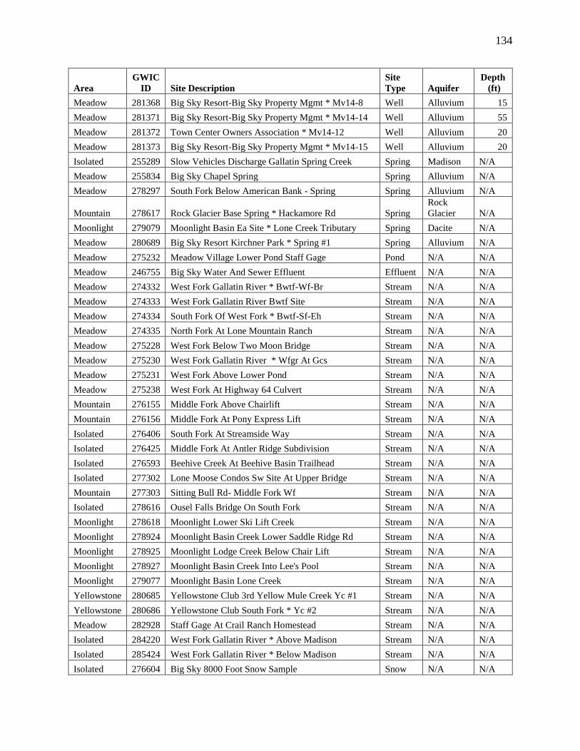
134
Area
GWIC
ID Site Description
Site
Type Aquifer
Depth
(ft)
Meadow 281368 Big Sky Resort-Big Sky Property Mgmt * Mv14-8 Well Alluvium 15
Meadow 281371 Big Sky Resort-Big Sky Property Mgmt * Mv14-14 Well Alluvium 55
Meadow 281372 Town Center Owners Association * Mv14-12 Well Alluvium 20
Meadow 281373 Big Sky Resort-Big Sky Property Mgmt * Mv14-15 Well Alluvium 20
Isolated 255289 Slow Vehicles Discharge Gallatin Spring Creek Spring Madison N/A
Meadow 255834 Big Sky Chapel Spring Spring Alluvium N/A
Meadow 278297 South Fork Below American Bank - Spring Spring Alluvium N/A
Mountain 278617 Rock Glacier Base Spring * Hackamore Rd Spring
Rock
Glacier N/A
Moonlight 279079 Moonlight Basin Ea Site * Lone Creek Tributary Spring Dacite N/A
Meadow 280689 Big Sky Resort Kirchner Park * Spring #1 Spring Alluvium N/A
Meadow 275232 Meadow Village Lower Pond Staff Gage Pond N/A N/A
Meadow 246755 Big Sky Water And Sewer Effluent Effluent N/A N/A
Meadow 274332 West Fork Gallatin River * Bwtf-Wf-Br Stream N/A N/A
Meadow 274333 West Fork Gallatin River Bwtf Site Stream N/A N/A
Meadow 274334 South Fork Of West Fork * Bwtf-Sf-Eh Stream N/A N/A
Meadow 274335 North Fork At Lone Mountain Ranch Stream N/A N/A
Meadow 275228 West Fork Below Two Moon Bridge Stream N/A N/A
Meadow 275230 West Fork Gallatin River * Wfgr At Gcs Stream N/A N/A
Meadow 275231 West Fork Above Lower Pond Stream N/A N/A
Meadow 275238 West Fork At Highway 64 Culvert Stream N/A N/A
Mountain 276155 Middle Fork Above Chairlift Stream N/A N/A
Mountain 276156 Middle Fork At Pony Express Lift Stream N/A N/A
Isolated 276406 South Fork At Streamside Way Stream N/A N/A
Isolated 276425 Middle Fork At Antler Ridge Subdivision Stream N/A N/A
Isolated 276593 Beehive Creek At Beehive Basin Trailhead Stream N/A N/A
Isolated 277302 Lone Moose Condos Sw Site At Upper Bridge Stream N/A N/A
Mountain 277303 Sitting Bull Rd- Middle Fork Wf Stream N/A N/A
Isolated 278616 Ousel Falls Bridge On South Fork Stream N/A N/A
Moonlight 278618 Moonlight Lower Ski Lift Creek Stream N/A N/A
Moonlight 278924 Moonlight Basin Creek Lower Saddle Ridge Rd Stream N/A N/A
Moonlight 278925 Moonlight Lodge Creek Below Chair Lift Stream N/A N/A
Moonlight 278927 Moonlight Basin Creek Into Lee's Pool Stream N/A N/A
Moonlight 279077 Moonlight Basin Lone Creek Stream N/A N/A
Yellowstone 280685 Yellowstone Club 3rd Yellow Mule Creek Yc #1 Stream N/A N/A
Yellowstone 280686 Yellowstone Club South Fork * Yc #2 Stream N/A N/A
Meadow 282928 Staff Gage At Crail Ranch Homestead Stream N/A N/A
Isolated 284220 West Fork Gallatin River * Above Madison Stream N/A N/A
Isolated 285424 West Fork Gallatin River * Below Madison Stream N/A N/A
Isolated 276604 Big Sky 8000 Foot Snow Sample Snow N/A N/A

135
Area
GWIC
ID Site Description
Site
Type Aquifer
Depth
(ft)
Mountain 277295 Big Sky Lone Moose Water Tank Snow Sample Snow N/A N/A
Meadow 277296 Big Sky Golf Course Picnic Area Snow Sample Snow N/A N/A
Mountain 283860 Cascade #6 Well Site Rain Sample Rain N/A N/A
Isolated 283861 Bucks T-4 Rainfall Sample Rain N/A N/A

136
10. Appendix C: Field and Water Isotope (18O and D) Data
GWIC
ID
Site
Type Aquifer
Water
Temp.
(°C)
Field
pH
Field SC
(µS/cm)
δ18O
(‰) δD (‰)
103496 Well Dacite N/A N/A N/A -20.0 -151.0
104510 Well Mowry 8.6 8.8 765.0 -20.4 -158.0
176326 Well Morrison 7.1 7.5 1084.0 -20.4 -158.0
176327 Well Morrison 7.6 7.7 398.4 -18.0 -140.0
192856 Well Kootenai 5.3 6.8 221.9 -20.3 -156.0
192865 Well Kootenai 7.3 7.7 354.0 -18.7 -143.0
192966 Well Kootenai 5.7 7.5 645.8 -19.7 -150.0
205931 Well Dacite 5.2 8.0 214.4 -19.7 -148.0
209445 Well Mowry 5.2 8.0 444.0 -19.3 -147.0
215507 Well Muddy 4.2 8.6 119.4 -19.0 -142.0
215510 Well Mowry 7.5 8.3 333.5 -19.2 -144.0
215510 Well Mowry 5.3 8.0 336.0 -18.9 -145.0
219966 Well Morrison 6.3 7.8 945.0 -19.2 -148.0
230689 Well Muddy 6.1 7.9 376.6 -19.7 -150.0
230803 Well Muddy 5.1 7.3 104.0 -19.5 -145.0
230804 Well Muddy 6.5 10.1 547.3 -20.6 -155.0
231031 Well Mowry 5.9 7.8 488.0 -19.0 -146.0
231745 Well Muddy 6.4 9.3 298.0 -20.4 -152.0
234783 Well Morrison 5.2 8.0 374.7 -19.1 -144.0
237292 Well Kootenai 9.7 7.7 497.6 -19.7 -153.0
239759 Well Kootenai 11.1 7.6 529.6 -20.5 -154.0
244347 Well Muddy 6.0 9.7 301.6 -19.4 -146.0
253676 Well Morrison 10.6 9.2 1332.0 -20.7 -157.0
259357 Well Muddy 5.8 9.0 334.4 -19.4 -145.0
259357 Well Muddy 5.8 9.6 331.0 -19.5 -150.0
259685 Well Muddy 7.8 9.5 700.1 -20.3 -154.0
259706 Well Muddy 9.2 8.8 663.2 -19.7 -149.0
262271 Well Morrison 7.8 8.6 592.0 -20.6 -154.0
275582 Well Muddy 6.0 8.4 1274.0 -20.1 -157.0
279062 Well Frontier 3.1 7.9 194.2 -18.7 -139.0
279080 Well Dacite N/A N/A N/A -19.5 -145.0
279080 Well Dacite 3.3 8.4 191.0 -19.0 -141.0
279082 Well Mowry N/A N/A N/A -19.8 -147.0
281359 Well Alluvium 8.1 7.6 770.0 -18.2 -144.0
281360 Well Alluvium 5.6 7.8 289.0 -18.6 -145.0
281362 Well Alluvium 6.5 7.8 127.1 -18.3 -140.0
281363 Well Alluvium 5.8 7.7 448.1 -19.2 -149.0

137
GWIC
ID
Site
Type Aquifer
Water
Temp.
(°C)
Field
pH
Field SC
(µS/cm)
δ18O
(‰) δD (‰)
281366 Well Alluvium 7.8 7.5 478.0 -18.7 -145.0
281367 Well Alluvium 7.3 7.3 472.2 -18.9 -148.0
281368 Well Alluvium 6.8 7.4 485.4 -18.6 -145.0
281371 Well Alluvium 7.5 7.5 452.0 -18.9 -148.0
281372 Well Alluvium 5.3 7.6 602.9 -18.4 -146.0
281373 Well Alluvium 7.6 7.7 477.0 -18.9 -148.0
255289 Spring Madison 13.8 7.8 450.0 -19.7 -149.0
255289 Spring Madison 14 7.7 465.6 -20.0 -149.0
255289 Spring Madison 14.1 7.9 385.3 -19.6 -150.0
255289 Spring Madison 14.1 N/A N/A -19.2 -148.0
255834 Spring Alluvium 11 7.2 726.0 -19.0 -145.0
278297 Spring Alluvium 9.9 7.5 898.0 -18.0 -141.0
278617 Spring
Rock
Glacier 1 8.2 52.2 -19.1 -145.0
278617 Spring
Rock
Glacier 2.9 7.8 64.2 -18.9 -144.0
278617 Spring
Rock
Glacier 1.4 7.5 63.0 -19.1 -142.0
279079 Spring Dacite N/A N/A N/A -19.1 -144.0
279079 Spring Dacite 2.3 8.1 177.0 -18.7 -139.0
280689 Spring Alluvium 15.6 7.9 1033.0 -18.7 -146.0
275232 Pond N/A 6.5 8.0 447.2 -20.0 -149.0
246755 Effluent N/A 17.5 8.1 714.0 -16.5 -134.0
274332 Stream N/A 0.7 8.3 346.2 -18.9 -145.0
274332 Stream N/A 4.7 8.7 281.4 -19.0 -147.0
274332 Stream N/A 6.1 8.4 147.6 -21.2 -153.0
274332 Stream N/A 6.8 8.2 131.0 -21.1 -153.0
274332 Stream N/A 7.5 8.6 126.9 -19.7 -148.0
274332 Stream N/A 9.9 8.2 205.8 -18.6 -144.0
274332 Stream N/A -0.1 8.3 409.2 -16.8 -141.0
274332 Stream N/A 11.1 9.0 252.9 -18.2 -140.0
274333 Stream N/A 6.4 8.8 260.9 -18.1 -145.0
274333 Stream N/A 2.1 8.4 360.4 -20.9 -151.0
274333 Stream N/A 4.9 8.5 284.7 -20.1 -150.0
274333 Stream N/A 5.4 8.2 131.1 -21.5 -155.0
274333 Stream N/A 5.9 8.1 112.0 -21.5 -155.0
274333 Stream N/A 7.4 8.4 97.8 -19.4 -148.0
274333 Stream N/A 10.5 8.1 172.6 -19.3 -147.0
274333 Stream N/A 12.2 8.6 272.6 -19.5 -146.0
274333 Stream N/A 11.7 8.8 237.1 -18.4 -141.0

138
GWIC
ID
Site
Type Aquifer
Water
Temp.
(°C)
Field
pH
Field SC
(µS/cm)
δ18O
(‰) δD (‰)
274333 Stream N/A 14.0 8.6 233.4 -18.3 -142.0
274334 Stream N/A 4.7 8.6 315.5 -19.4 -146.0
274334 Stream N/A 4.1 8.7 272.9 -20.6 -150.0
274334 Stream N/A 5.3 8.3 154.9 -21.3 -152.0
274334 Stream N/A 5.9 8.2 138.1 -21.2 -153.0
274334 Stream N/A 5.9 8.2 138.1 -21.2 -153.0
274334 Stream N/A 7.0 8.5 140.7 -19.1 -147.0
274334 Stream N/A 9.7 8.2 218.4 -18.8 -145.0
274334 Stream N/A 13.3 8.8 281.4 -19.3 -143.0
274334 Stream N/A 11.7 9.0 263.4 -18.2 -139.0
274335 Stream N/A 1.8 8.4 248.6 -20.1 -148.0
274335 Stream N/A 1.8 8.7 236.8 -19.7 -147.0
274335 Stream N/A 1.9 8.2 112.7 -21.9 -155.0
274335 Stream N/A 3.6 8.1 84.0 -21.2 -156.0
274335 Stream N/A 5.4 8.0 66.8 -19.6 -149.0
274335 Stream N/A 12.0 8.2 111.8 -19.4 -147.0
274335 Stream N/A -0.1 8.4 265.8 -18.0 -144.0
275228 Stream N/A 4.6 8.5 197.8 -17.9 -144.0
275228 Stream N/A 1.5 8.2 298.9 -20.9 -152.0
275228 Stream N/A 3.0 8.2 232.9 -20.5 -151.0
275228 Stream N/A 4.2 8.2 118.0 -21.5 -155.0
275228 Stream N/A 5.1 8.2 99.9 -21.3 -155.0
275228 Stream N/A 5.9 8.1 82.2 -19.5 -149.0
275228 Stream N/A 15.5 8.2 132.2 -19.1 -146.0
275228 Stream N/A 7.4 8.0 202.9 -19.0 -143.0
275228 Stream N/A 0.0 8.2 296.7 -16.1 -141.0
275228 Stream N/A 6.9 8.4 189.6 -18.4 -141.0
275230 Stream N/A 4.8 8.6 200.3 -18.1 -144.0
275230 Stream N/A 7.9 8.5 191.4 -18.4 -141.0
275231 Stream N/A 5.6 8.6 244.5 -17.9 -144.0
275231 Stream N/A 3.9 8.2 267.4 -19.8 -150.0
275231 Stream N/A 9.3 8.3 263.4 -19.4 -145.0
275231 Stream N/A 10.1 8.5 216.3 -18.4 -141.0
275238 Stream N/A 6.4 8.8 263.4 -18.5 -145.0
275238 Stream N/A 12.0 9.0 235.7 -18.4 -141.0
276155 Stream N/A 0.7 7.8 173.7 -20.4 -148.0
276156 Stream N/A 2.7 7.6 80.0 -21.1 -151.0
276156 Stream N/A 3.6 7.8 91.8 -21.0 -151.0
276156 Stream N/A 5.2 7.9 106.6 -19.1 -146.0

139
GWIC
ID
Site
Type Aquifer
Water
Temp.
(°C)
Field
pH
Field SC
(µS/cm)
δ18O
(‰) δD (‰)
276156 Stream N/A 6.3 7.8 108.0 -19.0 -145.0
276156 Stream N/A 0.3 7.8 115.4 -15.3 -135.0
276156 Stream N/A N/A N/A N/A -19.3 -144.0
276406 Stream N/A 9.1 8.3 220.4 -18.9 -145.0
276425 Stream N/A 3.5 8.2 119.6 -21.5 -155.0
276425 Stream N/A 7.9 8.1 106.8 -21.2 -154.0
276593 Stream N/A 1.6 7.8 119.2 -21.8 -155.0
276593 Stream N/A 1.9 8.0 77.5 -21.7 -156.0
276593 Stream N/A 8.9 8.1 87.8 -18.7 -144.0
276593 Stream N/A -0.1 8.1 176.2 -19.0 -144.0
277302 Stream N/A N/A N/A N/A -20.6 -149.0
277302 Stream N/A 1.7 8.3 210.4 -20.3 -150.0
277302 Stream N/A 2.8 8.1 119.4 -21.5 -155.0
277302 Stream N/A 4.6 8.1 105.6 -21.1 -154.0
277302 Stream N/A 13.5 8.5 133.9 -19.0 -145.0
277303 Stream N/A 5.2 7.8 151.1 -18.7 -144.0
277303 Stream N/A 4.4 7.7 92.0 -21.2 -153.0
277303 Stream N/A 5.5 7.9 102.6 -20.8 -151.0
277303 Stream N/A 11.0 7.8 108.8 -18.8 -144.0
278616 Stream N/A 9.5 8.3 141.9 -19.1 -146.0
278616 Stream N/A 15.0 8.5 214.8 -18.8 -144.0
278616 Stream N/A N/A N/A N/A -16.8 -145.0
278618 Stream N/A 6.0 8.1 130.7 -18.8 -144.0
278618 Stream N/A 6.2 8.4 144.0 -19.0 -140.0
278618 Stream N/A 4.9 8.9 177.6 -18.5 -140.0
278924 Stream N/A 3.9 7.9 89.3 -18.4 -146.0
278925 Stream N/A 4.9 8.1 111.4 -18.7 -146.0
278927 Stream N/A 11.1 8.3 88.3 -19.0 -148.0
278927 Stream N/A 11.8 8.2 98.1 -18.4 -140.0
279077 Stream N/A N/A N/A N/A -19.3 -145.0
280685 Stream N/A 1.8 8.1 214.7 -18.1 -138.0
280685 Stream N/A 7.0 8.5 133.0 -16.7 -131.0
280686 Stream N/A 2.3 8.2 201.2 -18.8 -142.0
280686 Stream N/A 8.2 8.6 153.0 -18.7 -141.0
282928 Stream N/A 9.6 8.5 206.8 -18.3 -141.0
284220 Stream N/A 13.6 8.5 235.6 -18.3 -142.0
284220 Stream N/A 11.6 N/A N/A -18.2 -140.0
285424 Stream N/A 11.7 N/A N/A -18.2 -139.0
276604 Precip N/A N/A N/A N/A -22.7 -167.0

140
GWIC
ID
Site
Type Aquifer
Water
Temp.
(°C)
Field
pH
Field SC
(µS/cm)
δ18O
(‰) δD (‰)
276604 Precip N/A N/A N/A N/A -22.9 -167.0
276604 Precip N/A 10.9 8.2 2.0 -20.4 -159.0
277295 Precip N/A N/A N/A N/A -20.8 -165.0
277296 Precip N/A N/A N/A N/A -25.1 -184.0
283860 Precip N/A N/A N/A N/A -13.6 -100.0
283861 Precip N/A 12.6 5.2 4.9 -13.6 -105.0

141
11. Appendix D: Raw Water Chemistry Data, Major Cations
J = Estimated quantity above detection limit but below reporting limit.
U = Undetected quantity below detection limit.
GWIC ID Ca (mg/L) Mg (mg/L) Na (mg/L) K (mg/L) Fe (mg/L) Mn (mg/L)
SiO2
(mg/L)
103496 3.09 0.56 58.02 0.98 <0.015 U <0.002 U 20.26
104510 0.89 0.14 148.81 <0.050 U <0.015 U 0.005 J 13.84
176326 110.15 47.50 77.35 9.59 0.125 J 0.098 J 6.71
176327 37.60 12.49 9.78 2.06 <0.015 U 0.006 J 9.55
192856 20.42 9.52 1.04 1.69 3.46 0.21 5.59
192865 44.81 12.69 9.24 1.05 <0.015 U <0.002 U 8.49
192966 60.50 20.85 36.17 4.55 0.13 0.08 5.13
205931 21.51 4.71 17.16 0.88 <0.015 U <0.002 U 11.79
209445 43.22 22.81 5.92 1.44 <0.015 U <0.002 U 13.75
215507 13.22 2.13 4.65 0.51 <0.015 U <0.002 U 8.07
215510 46.02 12.90 4.20 1.32 0.052 J 0.26 9.21
219966 9.72 1.30 195.27 0.70 <0.015 U <0.002 U 14.46
230689 35.54 9.02 22.72 0.62 0.18 0.30 13.44
230803 13.35 2.57 3.66 0.54 0.026 J 0.002 J 13.48
230804 0.54 0.020 J 111.40 0.110 J <0.015 U 0.002 J 11.33
231031 65.66 21.08 9.74 1.65 <0.015 U 0.046 J 12.67
231745 6.26 1.72 62.80 0.87 0.09 0.018 J 8.98
234783 39.51 14.93 5.60 2.14 0.18 0.011 J 6.96
237292 47.17 22.48 39.81 6.68 0.08 0.007 J 7.16
239759 56.62 22.72 27.62 5.36 0.11 0.16 6.73
244347 1.77 0.75 66.86 0.87 <0.015 U <0.002 U 13.86
253676 1.25 0.74 288.89 1.12 <0.038 U <0.005 U 10.06
259357 19.04 4.94 50.45 0.39 <0.015 U 0.05 10.17
259685 1.16 0.100 J 148.12 0.34 <0.015 U <0.002 U 7.13
259706 16.68 4.91 115.82 0.90 0.021 J 0.05 9.64
262271 12.13 4.81 128.59 3.54 0.13 0.009 J 6.83
275582 3.43 0.61 265.01 0.33 <0.038 U 0.046 J 12.05
279062 25.23 3.57 3.47 0.65 <0.015 U <0.002 U 5.48
279080 23.43 4.65 8.89 1.01 <0.015 U 0.003 J 5.73
281359 106.55 31.93 20.22 1.58 <0.015 U 0.009 J 15.73
281360 42.75 9.30 9.26 1.34 <0.015 U 0.002 J 10.42
281362 18.16 4.10 4.10 0.97 0.022 J <0.002 U 8.96
281363 66.84 14.76 16.53 2.04 <0.015 U 0.020 J 14.39
281366 75.10 16.51 13.28 1.41 <0.015 U 0.004 J 11.50
281367 75.24 17.55 10.00 2.31 <0.015 U <0.002 U 12.92
281368 77.09 16.87 13.08 1.42 0.017 J <0.002 U 11.20
281371 72.68 16.83 8.02 2.16 <0.015 U 0.005 J 12.66
281372 100.27 24.53 5.78 1.06 0.024 J 0.003 J 13.00
281373 79.41 17.76 7.50 2.11 <0.015 U <0.002 U 12.37
255289 56.84 21.75 4.73 1.31 <0.015 U <0.002 U 8.94

142
GWIC ID Ca (mg/L) Mg (mg/L) Na (mg/L) K (mg/L) Fe (mg/L) Mn (mg/L)
SiO2
(mg/L)
255289 58.45 22.67 5.28 1.34 0.031 J 0.05 9.87
278297 105.29 23.64 23.93 1.82 0.027 J <0.002 U 11.21
278617 8.46 1.17 1.92 0.48 <0.015 U <0.002 U 7.65
279079 26.02 5.24 2.50 0.68 <0.015 U <0.002 U 5.39
280689 119.87 31.12 54.65 2.06 <0.038 U <0.005 U 12.48
246755 39.78 10.00 70.54 13.34 <0.015 U 0.003 J 12.56
274332 39.31 11.19 11.74 1.39 <0.015 U 0.005 J 7.55
274332 19.19 4.95 3.23 0.82 <0.015 U 0.002 J 6.42
274332 17.30 4.50 2.17 0.57 0.036 J 0.003 J 6.13
274332 56.62 15.25 10.61 1.52 <0.015 U 0.004 J 7.55
274333 40.75 10.41 14.37 1.62 0.018 J 0.019 J 9.60
274333 16.36 3.81 4.30 0.93 0.058 J 0.006 J 7.59
274333 14.59 3.45 2.44 0.79 0.033 J 0.006 J 6.53
274334 38.96 10.54 8.73 1.28 <0.015 U <0.002 U 6.35
274334 20.52 5.47 2.48 0.71 0.028 J 0.002 J 6.06
274334 18.38 4.96 2.03 0.54 0.021 J <0.002 U 5.79
274334 18.28 4.89 1.99 0.62 0.016 J <0.002 U 5.85
274335 33.38 9.10 2.48 1.98 <0.015 U 0.005 J 6.13
274335 14.38 3.29 1.47 1.07 0.027 J <0.002 U 5.04
274335 11.63 2.65 0.96 0.79 0.018 J <0.002 U 4.74
274335 39.34 9.89 2.47 1.69 <0.015 U <0.002 U 6.91
275228 30.44 8.03 14.49 1.51 0.034 J 0.006 J 9.93
275228 13.35 3.09 3.44 0.85 0.052 J 0.003 J 8.58
275228 13.36 2.94 2.04 0.78 0.045 J 0.002 J 6.26
275228 39.56 9.32 8.86 1.36 0.015 J 0.012 J 9.22
275228 25.08 5.82 5.03 1.06 <0.015 U 0.029 J 7.44
275238 31.68 7.52 6.24 1.17 <0.015 U 0.015 J 6.77
276156 9.70 1.50 2.42 0.73 0.040 J <0.002 U 9.47
276156 12.75 1.80 2.20 0.58 <0.015 U <0.002 U 9.84
276156 15.43 2.75 3.21 0.83 <0.015 U <0.002 U 9.66
276156 15.62 2.28 2.29 0.75 <0.015 U <0.002 U 9.83
276425 13.14 3.17 3.42 0.67 0.047 J 0.003 J 8.26
276425 14.64 3.05 2.37 0.59 0.033 J 0.003 J 7.38
276593 15.08 3.54 0.80 0.74 0.045 J 0.005 J 5.65
276593 11.41 2.27 0.21 0.42 0.024 J <0.002 U 4.24
276593 26.49 6.17 1.22 0.81 0.036 J 0.009 J 4.76
277302 26.39 6.86 14.99 1.30 0.024 J <0.002 U 9.63
277302 14.13 3.09 2.82 0.70 0.055 J 0.004 J 7.78
277302 14.36 3.03 1.97 0.54 0.052 J 0.005 J 6.74
277303 8.52 2.33 3.97 0.67 0.071 J 0.012 J 8.65
278618 20.23 3.30 4.57 0.68 <0.015 U <0.002 U 5.96
278927 7.93 2.30 7.80 0.62 0.10 0.006 J 10.00
280685 18.81 4.11 2.37 0.50 <0.015 U <0.002 U 5.95
280686 22.71 4.41 2.51 0.48 <0.015 U <0.002 U 6.85
276604 0.27 <0.020 U 0.020 J <0.050 U <0.015 U <0.002 U 0.060 J

143
12. Appendix E: Raw Water Chemistry Data, Major Anions
J = Estimated quantity above detection limit but below reporting limit.
U = Undetected quantity below detection limit.
GWIC
ID
HCO3
(mg/L)
CO3
(mg/L)
SO4
(mg/L) Cl (mg/L)
NO3-N
(mg/L) F (mg/L)
OPO4-P
(mg/L)
103496 113.25 20.69 5.19 4.62 0.06 0.28 <0.020 U
104510 333.71 18.79 41.36 12 0.1 0.28 <0.020 U
176326 466.32 0.00 267.80 1.62 <0.010 U 0.86 <0.020 U
176327 177.30 0.00 20.17 14.40 0.47 0.18 <0.020 U
192856 103.20 0.00 10.22 3.93 <0.010 U 0.22 <0.020 U
192865 179.87 0.00 20.93 17.59 0.56 0.14 <0.020 U
192966 361.69 0.00 27.79 0.68 <0.010 U 0.64 0.040 J
205931 90.15 0.00 6.62 9.44 0.27 0.23 <0.020 U
209445 154.77 0.00 10.80 69.48 0.20 0.15 0.020 J
215507 53.91 0.00 9.82 0.58 0.18 0.10 <0.020 U
215510 139.11 0.00 51.26 1.70 <0.010 U 0.27 <0.020 U
219966 306.75 0.00 25.84 110.20 0.43 0.54 <0.020 U
230689 177.10 0.00 32.84 0.59 <0.010 U 0.22 <0.020 U
230803 53.53 0.00 9.20 1.88 0.37 0.12 <0.020 U
230804 153.47 63.74 12.70 0.55 <0.010 U 0.75 <0.020 U
231031 229.02 0.00 90.41 0.99 <0.010 U 0.17 <0.020 U
231745 180.13 8.68 8.48 0.63 <0.010 U 0.17 <0.020 U
234783 180.65 0.00 21.06 6.41 0.29 0.21 <0.020 U
237292 271.18 0.00 79.44 3.37 0.47 0.96 <0.020 U
239759 284.11 0.00 65.72 0.91 <0.010 U 0.81 <0.020 U
244347 118.73 28.50 7.49 4.12 0.11 0.26 <0.020 U
253676 614.85 35.57 31.48 16.83 <0.010 U 2.58 <0.020 U
259357 149.35 11.97 39.88 0.70 <0.010 U 0.25 <0.020 U
259685 265.27 28.17 1.110 J 10.51 <0.010 U 19.93 <0.020 U
259706 290.51 7.36 70.86 1.08 <0.010 U 1.46 <0.020 U
262271 336.71 0.00 2.280 J 26.37 <0.010 U 3.63 <0.020 U
275582 498.01 3.84 188.60 2.77 <0.010 U 0.79 <0.020 U
279062 78.91 0.00 22.01 0.460 J 0.40 0.10 <0.020 U
279080 102.73 0.00 21.24 0.51 0.25 0.14 <0.020 U
281359 355.56 0.00 16.40 95.07 4.91 0.14 0.050 J
281360 171.45 0.00 11.08 12.51 0.84 0.13 <0.020 U
281362 85.27 0.00 4.14 1.84 0.08 0.13 0.030 J
281363 271.07 0.00 17.78 23.16 0.42 0.14 0.020 J
281366 288.65 0.00 19.16 23.72 1.67 0.14 <0.020 U
281367 299.46 0.00 13.14 17.61 1.86 0.15 <0.020 U
281368 290.53 0.00 19.64 24.96 1.48 0.16 <0.020 U
281371 283.93 0.00 12.40 19.40 1.30 0.13 <0.020 U
281372 377.97 0.00 16.70 21.24 6.27 0.11 <0.020 U
281373 299.38 0.00 12.15 21.00 2.08 0.12 <0.020 U
255289 179.03 0.00 106.50 1.62 0.11 0.48 <0.020 U

144
GWIC
ID
HCO3
(mg/L)
CO3
(mg/L)
SO4
(mg/L) Cl (mg/L)
NO3-N
(mg/L) F (mg/L)
OPO4-P
(mg/L)
255289 173.17 0.00 110.40 1.92 0.16 0.53 <0.020 U
278297 349.40 0.00 26.01 69.86 4.94 0.12 0.020 J
278617 34.16 0.00 5.62 0.54 0.25 0.13 <0.020 U
279079 92.12 0.00 21.87 0.470 J 0.31 0.09 <0.020 U
280689 378.39 0.00 39.45 151.10 2.98 0.10 <0.020 U
246755 209.95 0.00 30.34 95.82 0.82 0.14 1.43
274332 159.47 0.00 28.94 21.23 0.41 0.13 0.030 J
274332 85.15 0.00 6.99 2.99 0.14 0.11 <0.020 U
274332 79.17 0.00 6.31 1.41 0.12 0.09 <0.020 U
274332 226.96 1.90 28.98 10.16 0.38 0.16 <0.020 U
274333 163.25 0.00 14.97 29.91 0.52 0.13 <0.020 U
274333 71.11 0.00 5.34 4.78 0.15 0.10 <0.020 U
274333 67.47 0.00 4.45 2.30 0.13 0.09 <0.020 U
274334 149.15 1.79 30.01 14.34 0.22 0.13 <0.020 U
274334 91.01 0.00 7.86 2.08 0.14 0.10 <0.020 U
274334 83.72 0.00 7.74 1.10 0.09 0.09 <0.020 U
274334 84.05 0.00 7.27 1.04 0.11 0.09 <0.020 U
274335 153.45 0.00 10.16 1.93 0.09 0.13 <0.020 U
274335 70.74 0.00 5.20 0.61 0.11 0.09 <0.020 U
274335 54.03 0.00 2.94 0.480 J 0.07 0.08 <0.020 U
274335 164.75 0.00 9.44 1.28 0.12 0.13 <0.020 U
275228 118.94 0.00 13.46 31.14 0.16 0.14 <0.020 U
275228 63.98 0.00 4.83 4.01 0.11 0.09 <0.020 U
275228 61.21 0.00 3.84 1.67 0.09 0.09 <0.020 U
275228 163.32 0.00 13.25 9.76 0.06 0.12 <0.020 U
275228 106.70 0.00 7.29 4.96 0.05 0.12 <0.020 U
275238 122.18 6.09 8.35 8.39 0.14 0.12 <0.020 U
276156 40.10 0.00 5.89 1.21 0.25 0.11 <0.020 U
276156 45.86 0.00 8.76 0.79 0.23 0.11 <0.020 U
276156 48.54 0.00 13.89 0.96 0.28 0.11 0.030 J
276156 53.75 0.00 12.82 0.68 0.26 0.12 <0.020 U
276425 54.66 0.00 3.75 5.02 0.13 0.09 <0.020 U
276425 64.52 0.00 3.74 2.40 0.13 0.09 <0.020 U
276593 69.76 0.00 3.66 0.50 0.10 0.10 <0.020 U
276593 46.01 0.00 2.430 J 0.390 J 0.09 0.08 <0.020 U
276593 106.61 0.00 6.14 0.460 J 0.030 J 0.10 0.020 J
277302 106.81 0.00 9.56 29.34 0.14 0.12 <0.020 U
277302 65.74 0.00 3.66 4.47 0.15 0.09 <0.020 U
277302 62.30 0.00 3.79 2.20 0.14 0.09 <0.020 U
277303 44.55 0.00 2.50 6.06 0.13 0.09 <0.020 U
278618 76.31 0.00 16.59 0.50 0.19 0.10 <0.020 U
278927 60.34 0.00 1.480 J 0.63 <0.010 U 0.11 <0.020 U
280685 73.80 0.00 12.26 0.490 J 0.05 0.10 <0.020 U
280686 88.59 0.00 10.30 0.99 0.12 0.09 <0.020 U
276604 1.56 0.00 1.200 J 0.54 0.030 J <0.010 U <0.020 U

145
13. Appendix F: Raw Water Chemistry Data, Select Constituents
J = Estimated quantity above detection limit but below reporting limit.
U = Undetected quantity below detection limit.
GWIC ID Al (µg/L) As (µg/L) Mo (µg/L)
Total Dissolved Solids
(mg/L)
Hardness
(mg/L) SAR
103496 <2.000 U 0.8 2.14 169.315 10.0207 7.973
104510 <2.000 U 0.49 2.99 400.562 2.7986 38.758
176326 <5.000 U 0.840 J 19.94 752.21 470.55 1.54
176327 <2.000 U 0.390 J 1.44 193.31 145.30 0.36
192856 <2.000 U <0.100 U 0.450 J 106.69 90.17 0.05
192865 <2.000 U 0.310 J 3.89 204.20 164.12 0.31
192966 <2.000 U 0.360 J 0.87 335.68 236.89 1.02
205931 <2.000 U 4.20 1.94 116.56 73.10 0.87
209445 <2.000 U 0.380 J 0.76 243.39 201.81 0.18
215507 8.400 J 0.390 J 1.21 66.99 41.78 0.34
215510 <2.000 U <0.100 U 0.59 194.39 168.01 0.13
219966 <2.000 U 1.49 5.55 509.27 29.62 15.59
230689 <2.000 U 2.50 1.64 202.75 125.87 0.89
230803 <2.000 U 0.220 J 0.75 71.53 43.91 0.26
230804 3.660 J <0.100 U 1.87 276.91 1.35 41.60
231031 <2.000 U <0.100 U 0.310 J 315.55 250.72 0.27
231745 <2.000 U <0.100 U 0.61 187.65 22.71 5.75
234783 <2.000 U <0.100 U 2.43 185.66 160.11 0.21
237292 <2.000 U <0.100 U 1.78 340.15 210.31 1.20
239759 <2.000 U 0.230 J 1.48 327.28 234.90 0.80
244347 2.650 J 18.62 2.13 183.14 7.51 10.64
253676 <5.000 U <0.250 U <0.250 U 691.95 6.17 50.64
259357 <2.000 U 1.80 3.00 210.38 67.88 2.64
259685 4.180 J <0.100 U 1.62 345.70 2.90 37.84
259706 16.67 0.43 6.17 371.96 61.86 6.42
262271 3.440 J 0.50 2.41 352.95 50.09 7.93
275582 <5.000 U 0.660 J 9.36 723.36 11.08 34.65
279062 <2.000 U 0.40 0.480 J 98.72 77.69 0.15
279080 <2.000 U 0.72 1.69 116.82 77.64 0.44
281359 2.190 J 0.340 J 1.42 467.86 397.48 0.44
281360 2.740 J 0.81 1.02 181.29 145.03 0.33
281362 33.85 0.46 0.99 84.17 62.22 0.22
281363 12.87 0.290 J 0.95 289.12 227.65 0.49
281366 2.770 J 0.340 J 2.06 304.98 255.48 0.35
281367 4.820 J 0.360 J 0.59 298.08 260.11 0.27
281368 2.770 J 0.340 J 1.43 308.31 261.93 0.35
281371 <2.000 U 0.290 J 0.440 J 284.41 250.75 0.22
281372 <2.000 U <0.100 U 0.320 J 375.01 351.34 0.14
281373 2.600 J 0.230 J 0.260 J 301.46 271.39 0.21
255289 <2.000 U 1.09 1.66 290.77 231.45 0.14

146
GWIC ID Al (µg/L) As (µg/L) Mo (µg/L)
Total Dissolved Solids
(mg/L)
Hardness
(mg/L) SAR
255289 33.62 1.17 1.20 295.40 239.26 0.14
278297 <2.000 U 0.280 J <0.100 U 438.85 360.21 0.55
278617 2.470 J 0.240 J 0.85 43.38 25.94 0.17
279079 <2.000 U 0.240 J 0.430 J 107.58 86.54 0.14
280689 <5.000 U <0.250 U <0.250 U 599.20 427.41 1.16
246755 27.73 1.03 21.35 378.27 140.49 2.61
274332 12.64 0.300 J 0.74 199.84 144.22 0.43
274332 8.970 J 0.340 J 0.430 J 86.01 68.29 0.16
274332 52.35 0.270 J 0.430 J 76.77 61.72 0.11
274332 <2.000 U 0.300 J 1.41 245.69 204.15 0.34
274333 4.960 J 0.43 0.61 203.46 144.60 0.51
274333 57.47 0.60 0.57 78.20 56.53 0.23
274333 33.12 0.340 J 0.350 J 67.08 50.63 0.12
274334 19.59 0.260 J 0.85 184.92 140.67 0.33
274334 32.84 0.300 J 0.480 J 89.85 73.75 0.10
274334 29.26 0.250 J 0.420 J 82.75 66.31 0.11
274334 25.64 0.230 J 0.440 J 81.58 65.77 0.11
274335 <2.000 U 0.42 0.440 J 139.85 120.81 0.08
274335 44.06 0.43 <0.100 U 65.69 49.45 0.06
274335 33.48 0.310 J 0.290 J 50.91 39.95 0.07
274335 <2.000 U 0.44 1.03 151.51 138.94 0.07
275228 22.94 0.43 0.55 167.12 109.06 0.58
275228 59.25 0.42 0.290 J 70.03 46.05 0.19
275228 36.15 0.320 J 0.300 J 61.39 45.46 0.13
275228 <2.000 U 0.380 J 1.01 171.18 137.14 0.33
275228 <2.000 U 0.44 0.64 108.61 86.58 0.23
275238 <2.000 U 0.43 0.52 135.30 110.06 0.25
276156 62.85 0.71 0.52 49.97 30.39 0.16
276156 25.21 0.59 0.62 60.24 39.25 0.14
276156 <2.000 U 0.58 1.23 71.33 49.85 0.18
276156 <2.000 U 0.56 0.440 J 71.50 48.39 0.13
276425 55.36 0.390 J 0.420 J 64.46 45.86 0.19
276425 40.44 0.330 J 0.310 J 65.75 49.11 0.12
276593 55.67 0.230 J <0.100 U 66.16 52.23 0.06
276593 32.04 0.210 J <0.100 U 40.37 37.83 0.00
276593 <2.000 U <0.100 U 0.55 98.37 91.54 0.05
277302 46.41 0.380 J 0.52 151.01 94.13 0.67
277302 71.96 0.340 J <0.100 U 69.80 48.00 0.19
277302 49.80 0.330 J 0.300 J 63.98 48.33 0.13
277303 75.91 0.350 J <0.100 U 56.09 30.86 0.31
278618 <2.000 U 0.380 J 0.68 90.97 64.10 0.27
278927 50.23 0.65 <0.100 U 59.84 29.27 0.64
280685 7.060 J <0.100 U <0.100 U 80.37 63.89 0.11
280686 2.630 J 0.270 J 0.56 91.96 74.86 0.15
276604 7.560 J <0.100 U <0.100 U 2.26 0.67 0.00

147
14. Appendix G: Stiff Diagrams for Each Water Quality Sample
Labeled with GWIC ID, Sample Date, and Site Type (groundwater samples by unit).

148

149

150

151

152

153

154
Mtn Village

155

156

157
Mtn Village

158

159

160

161

162

163

164

165

166

167
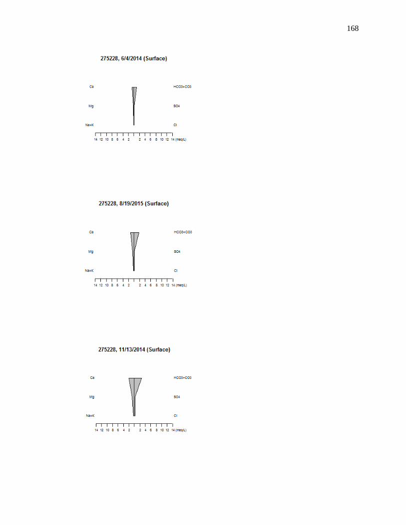
168

169

170

171

172

173

174

175