Transactions of the ASABE

Vol. 55(1): 137-147 � 2012 American Society of Agricultural and Biological Engineers ISSN 2151-0032 137

DETERMINING NUTRIENT AND SEDIMENT

CRITICAL SOURCE AREAS WITH SWAT:EFFECT OF LUMPED CALIBRATION

R. Niraula, L. Kalin, R. Wang, P. Srivastava

ABSTRACT. In many watershed modeling studies, due to limited data, model parameters for flow, sediment, and nutrients arecalibrated and validated against observed data only at the watershed outlet. Model parameters are adjusted systematicallyfor the entire watershed to obtain the closest match between the model‐simulated and observed data at the watershed outlet(lumped calibration). It is hypothesized that the relative loadings of pollutants and/or sediments contributed by eachcomputational unit are not affected by this calibration procedure. In other words, areas generating relatively higher pollutantloads with an uncalibrated model will still generate relatively higher loads after calibration. This study explored the effectof lumped calibration of the Soil and Water Assessment Tool (SWAT) on locations of sediment and nutrient critical source areas(CSAs). Two watersheds in Alabama with differing size, topography, hydrology, and land use/cover characteristics were usedto study the variations in locations of sediment, total phosphorus (TP), and total nitrogen (TN) CSAs identified by calibratedand uncalibrated SWAT models. Identified CSAs for sediment, TP, and TN were mostly the same with and without thecalibration of the model in both watersheds. This study thus concluded that lumped calibration of the SWAT model using dataat the watershed outlet has little effect on the locations of CSAs. Based on the results from these two watersheds, it was furtherconcluded that SWAT can be used without calibration for identification of CSAs in watersheds that lack sufficient data formodel calibration, but not for all other modeling purposes. More studies are encouraged to support these findings.

Keywords. Critical source area, Model calibration, Nutrient, Sediment, SWAT, Watershed.

onpoint‐source (NPS) pollution, unlike pollutionfrom specific point sources, such as dischargefrom industries and wastewater treatment plants,originates from numerous diffuse sources. It is

caused by natural and anthropogenic pollutants from agricul‐tural lands, urban areas, construction sites, forested lands,and pasture lands (USEPA, 2010). Major agricultural activi‐ties that are responsible for NPS pollution include poorlymanaged animal feeding operations, overgrazing, frequentplowing, and excessive application of fertilizers and pesti‐cides (USEPA, 2002). Construction and use of roads are theprime sources of NPS pollution from forest areas. Urbaniza‐tion enhances the variety and quantity of pollutants carriedinto water bodies (USEPA, 2002). Land uses such as lawns,parking lots, roofs, roads, and streets located in the residen‐tial, commercial, and industrial portions of urban areas are re‐

Submitted for review in June 2011 as manuscript number SW 9240;approved for publication by the Soil & Water Division of ASABE inNovember 2011.

The authors are Rewati Niraula, Graduate Student, Department ofHydrology and Water Resources, University of Arizona, Tucson, Arizona;Latif Kalin, Associate Professor, School of Forestry and Wildlife Sciences,Auburn University, Auburn, Alabama; Ruoyu Wang, Graduate Student,Department of Agricultural and Biological Engineering, PurdueUniversity, West Lafayette, Indiana; and Puneet Srivastava, ASABEMember, Associate Professor, Department of Biosystems Engineering,Auburn University, Auburn, Alabama. Corresponding author: LatifKalin, School of Forestry and Wildlife Sciences, Auburn University, 602Duncan Drive, Auburn, AL 36849; phone: 334‐844‐4671; fax: 334‐844‐1084; e‐mail: kalinla@auburn.edu.

sponsible for most of the phosphorus and heavy metal NPSpollution in urban watersheds (Bannerman et al., 1993).

Nonpoint‐source pollution is considered the principalcontributor of nitrogen (N) and phosphorus (P) to most sur‐face waters (USEPA, 2004). Excessive N and P cause eutro‐phication of lakes and reservoirs (USEPA, 2004). Approxi-mately 82% of N and 84% of P discharge to U.S. surface wa‐ter bodies come from nonpoint sources (Carpenter et al.,1998). In addition, the spatial distribution of sediment, P, andN sources is not homogeneous across a watershed (Ballantineet al., 2009). While some areas of a watershed are more proneto erosion and contribute larger amounts of sediment, otherparts of the watershed contribute little to overall load. Sometypically small and well‐defined areas contribute much of thesediment, P, and N into the watershed outflow (Walter et al.,2000; Pionke et al., 2000) and over relatively short periods(Dillon and Molot, 1997; Heathwaite et al., 2005). The criti‐cal sources of sediment associated with P are those hydrolog‐ically active areas that overlap with easily erodible soil withhigh P concentrations (Pionke et al., 2000; Heathwaite et al.,2005; Ballantine et al., 2009). These source areas are oftenlocated in relatively small definable areas near the streams(Walter et al., 2000, Russell et al., 2000; Gburek et al., 2002;Agnew et al., 2006; Walter et al., 2009; Ballantine et al.,2009). Thus, not all parts of a watershed are equally criticaland responsible for producing high amounts of sediment andnutrient loads (Ouyang et al., 2008). Some unique combina‐tions of soil, land use/cover, and topography are responsiblefor contributing higher sediment, N, and P loads. These areknown as critical source areas (CSAs). When resources arelimited, management should be directed toward CSAs

N

138 TRANSACTIONS OF THE ASABE

(Smith et al., 2001). Management practices implemented inthese targeted areas have the potential to be more effective attreating larger quantities of pollution (White et al., 2009).

CSAs are best identified through field investigations andsource tracking techniques, such as fingerprinting, which re‐quire tremendous labor and financial resources. Therefore,distributed watershed models are commonly used to locateCSAs. In most watershed modeling studies, models are cali‐brated for flow, sediment, or nutrients using observed data atone or two locations, generally at the watershed outlet (Chuet al., 2004; Hao et al., 2005; Santhi et al., 2006; Ouyang etal., 2008; Ahl et al., 2008; Kumar and Marwade, 2009). Thisis the case even with distributed models, in which model pa‐rameters for the entire watershed are adjusted, without ade‐quate calibration and validation at the subwatershed level, toensure that the model simulations match the observed data atthe outlet (Santhi et al., 2008). This means that parametersare systematically changed without actually making use ofthe distributed nature of the models, which is known aslumped calibration. The most common reason for this ap‐proach is the lack of observed data at various locations insidethe watershed (Santhi et al., 2008). If a lumped calibration re‐sults in a systematic increase or decrease in loadings from allareas, or if there is a monotonic relationship between modelparameters and model outputs, then the locations of CSAsshould not be affected by the calibration process.

The Soil and Water Assessment Tool (SWAT) (Arnold etal., 1998) is one of the most commonly used watershed mod‐els for predicting locations of CSAs in watersheds (Tripathiet al., 2003; Ouyang et al., 2008; Kalin and Hantush, 2009;Busteed et al., 2009; White et al., 2009; Singh et al., 2011).Although Santhi et al. (2001) stated that SWAT was devel‐oped for use in large uncalibrated watersheds, it is typicallycalibrated to improve performance. The SWAT model hasbeen used around the world for various purposes, includingmodeling daily streamflow (Spruill et al., 2000), predictingsediment and P (Kirsh et al., 2002; Veith et al., 2005), and de‐termining the impacts of urbanization on hydrology (Kalinand Hantush, 2006; Jha et al., 2007), the impacts of land useand climate change (Wang et al., 2008), and the impacts ofmanagement practices (Santhi et al., 2001; Vache et al.,2002).

There are limited studies reported in the literature thatused the SWAT model without calibration. Some studies usedSWAT in an uncalibrated mode to eliminate the bias causedby parameter optimization for modeling streamflow (Rosen‐thal et al., 1995; Heathman et al., 2008). Others used SWATin the uncalibrated mode to predict changes in water yield ina large river basin resulting from doubled CO2 concentration(Stone et al., 2001), to estimate surface water quality impactsfrom riparian buffers (Qiu and Prato, 2001), and to study theimpacts of soil and land use/cover datasets on simulated flow(Heathman et al., 2009).

Previous studies on identification of CSAs relied on bothcalibrated and uncalibrated watershed models. Yet, to thebest of our knowledge, no study has explored how the loca‐tions of CSAs are affected due to a calibrated vs. uncalibratedmodel. When model parameters are systematically adjustedover the entire watershed, the relative loadings of pollutantsand/or sediments contributed by each computational unit arepotentially not affected. This study thus hypothesizes that thelocations of CSAs do not change significantly due to lumpedcalibration. Calibrated and uncalibrated SWAT models were

used in two watersheds with different characteristics to iden‐tify and compare the locations of sediment, total phosphorus(TP), and total nitrogen (TN) CSAs.

MATERIALS AND METHODSSTUDY AREA

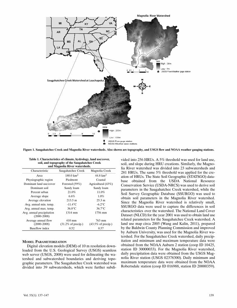
Two watersheds differing in size, physiographic charac‐teristics, land use/cover composition, climate, and hydrology(table 1) were selected for this study to test the above hypoth‐esis. The Saugahatchee Creek watershed (fig. 1) is part of theLower Tallapoosa basin in eastern Alabama. Although a ma‐jor portion of the watershed lies in the Piedmont physio‐graphic province, a small portion of the watershed is in theCoastal Plains province. The watershed is comprised of59.0% forested land, 21.0% urban area, 9.4% agriculturalland (hay/pasture and row crops), and 6.8% grassland(NLCD, 2001). The elevation ranges between 158 m and255�m with an average elevation of 213.5 m. The MagnoliaRiver watershed (fig. 1) is located on the Gulf of Mexico inBaldwin County, southern Alabama, and drains to WeeksBay, a sub‐estuary to Mobile Bay. It is dominantly agricultur‐al land (43.0%), followed by pasture (25.0%), wetland(11.5%), urban (11.0%), and forest (8.2%) (NLCD, 2001).Unlike the Saugahatchee Creek watershed, this watershed isrelatively flat.

SWAT MODELThe Soil Water Assessment Tool (SWAT) is a watershed‐

scale, continuous, semi‐distributed watershed model (Arnoldet al., 1998). Although the model has been described as physi‐cally based (Neitsch et al., 2005; Gassman et al., 2007; De‐bele et al., 2009), process‐based (Confesor and Whittaker,2007; Ekstrand et al., 2010), and physical process‐based(Behera and Panda, 2006), it would be best to describe it asa quasi‐process‐based model because it includes several em‐pirical relationships (e.g., the SCS CN method for runoff, andMUSLE for soil erosion). It was primarily developed to pre‐dict the impact of management practices on water, sediment,and agricultural chemicals in watersheds comprising differ‐ent soils, land use, and management conditions over long pe‐riods of time (Neitsch et al., 2005). The major model inputsare topography, soil properties, land use/cover type, weather/climate, and land management practices. The SWAT modelrequires the watershed to be subdivided into several subwa‐tersheds, which are further divided into hydrological re‐sponse units (HRUs) according to topography, land use, andsoil. Surface runoff from daily precipitation is estimated witha modification of the SCS curve number method (USDA,1972). Runoff from all HRUs in the subwatershed yields thetotal subwatershed discharge.

In SWAT, erosion and sediment yields from each HRU arepredicted based on the modified soil loss equation (MUSLE)developed by Williams (1975). Channel sediment is routedbased on the modified Bagnold's sediment transport equation(Bagnold, 1977). SWAT has complex N and P cycles in whichmineralization, decomposition, and immobilization are im‐portant processes. Organic N and P transport with sedimentand runoff is calculated with a loading function (Williamsand Hann, 1978). Neitsch et al. (2005) provide a detailed de‐scription of the SWAT model.

139Vol. 55(1): 137-147

Figure 1. Saugahatchee Creek and Magnolia River watersheds. Also shown are topography, and USGS flow and NOAA weather gauging stations.

Table 1. Characteristics of climate, hydrology, land use/cover,soil, and topography of the Saugahatchee Creek

and Magnolia River watersheds.Characteristic Saugahatchee Creek Magnolia Creek

Area 180.0 km2 44.8 km2

Physiographic region Piedmont CoastalDominant land use/cover Forested (59%) Agricultural (43%)

Dominant soil Sandy loam Sandy loamPercent urban 21.0% 11.0%Average slope 6.6% 1.0%

Average elevation 213.5 m 25.3 mAvg. annual min. temp. ‐11.4°C ‐6.2°CAvg. annual max. temp. 36.8°C 36.7°C

Avg. annual precipitation (2000‐2008)

1314 mm 1756 mm

Average annual flow (2000‐2008)

410 mm (31.2% of precip.)

763 mm(43.5% of precip.)

Baseflow index 0.52 0.57

MODEL PARAMETERIZATION

Digital elevation models (DEM) of 10 m resolution down‐loaded from the U.S. Geological Survey (USGS) seamlessweb server (USGS, 2008) were used for delineating the wa‐tershed and subwatershed boundaries and deriving topo‐graphic parameters. The Saugahatchee Creek watershed wasdivided into 39 subwatersheds, which were further subdi‐

vided into 256 HRUs. A 5% threshold was used for land use,soil, and slope during HRU creations. Similarly, the Magno‐lia River watershed was divided into 23 subwatersheds and281 HRUs. The same 5% threshold was applied for the cre‐ation of HRUs. The State Soil Geographic (STATSGO) data‐base obtained from the USDA National ResourceConservation Service (USDA‐NRCS) was used to derive soilparameters in the Saugahatchee Creek watershed, while theSoil Survey Geographic Database (SSURGO) was used toobtain soil parameters in the Magnolia River watershed.Since the Magnolia River watershed is relatively small,SSURGO data were used to capture the differences in soilcharacteristics over the watershed. The National Land CoverDataset (NLCD) for the year 2001 was used to obtain land userelated parameters for the Saugahatchee Creek watershed. Aland use map circa 2005 (Wang and Kalin, 2011), preparedby the Baldwin County Planning Commission and improvedby Auburn University, was used for the Magnolia River wa‐tershed. For the Saugahatchee Creek watershed, daily precip‐itation and minimum and maximum temperature data wereobtained from the NOAA Auburn 2 station (coop ID 10425,station ID 30000033). For the Magnolia River watershed,daily precipitation data were obtained from the USGS Mag‐nolia River station (USGS 02378300). Daily minimum andmaximum temperature data were obtained from the NOAARobertsdale station (coop ID 016988, station ID 20000359).

140 TRANSACTIONS OF THE ASABE

Table 2. Adjusted parameters for model calibration.

Parameter DescriptionsDefaultValue

Calibrated Values[a]

Saugahatchee Magnolia

CN2 Initial SCS runoff curve number for moisture AMC‐II Varies ‐5 +5ESCO Soil evaporation compensation factor 0.95 0.2 1

GWQMN (mm) Threshold depth of water in shallow aquifer required for the return flow to occur 0 1200 ‐‐GW_DELAY (days) Groundwater delay 31 ‐‐ 93

REVAPMN (mm) Threshold depth of water in the shallow aquifer for revap to occur 1 ‐‐ 500ALPHA_BF (days) Baseflow alpha factor 0.048 ‐‐ 0.015

SOL_AWC (mm mm‐1) Available water capacity of soil layer Varies ‐‐ ‐0.04SURLAG Surface runoff lag time 4 1 0.5

SPEXP Exponent parameter for calculating sediment re‐entrained in channel sediment routing 1 1.5 0.5PRF Peak rate adjustment factor for sediment routing in the main channel 1 1.97 0.6

ADJ_PKR Peak rate adjustment factor for sediment routing in the subbasins 0 2 ‐‐USLE_C (AGRR) USLE crop factor for agricultural land 0.2 ‐‐ 0.05

PPERCO Phosphorus percolation coefficient 10 17.5 17.5PHOSKD Phosphorus soil partitioning coefficient 175 200 200P‐UPDIS Phosphorus uptake distribution factor 20 80 100

PSP Phosphorus sorption coefficient 0.4 0.7 0.7SOL_LABP (mg kg‐1) Initial soluble P concentration in surface soil layer 0 12 3

NPERCO Nitrogen percolation coefficient 0.2 1 1SOL_NO3 (mg kg‐1) Initial NO3 concentration in the soil 0 21 ‐‐

BC1 Rate constant for biological oxidation of NH4 to NO2 in the reach 0.55 ‐‐ 1BC2 Rate constant for biological oxidation of NO2 to NO3 in the reach 1.1 ‐‐ 2BC3 Rate constant for hydrolysis of organic N to NH4 in the reach 0.21 ‐‐ 0.4BC4 Rate constant for mineralization of organic P to mineral P in the reach 0.35 ‐‐ 0.1RCN Concentration of nitrogen in rainfall 1 ‐‐ 2RS4 Organic P settling rate in reach at 20°C 0.05 ‐‐ 0.1RS5 Rate coefficient for organic N settling 0.05 ‐‐ 0.001

[a] “+” or “‐” indicates increase or reduction of the default value by the given amount; if there is no sign, then the value shown is the final calibratedvalue; “‐‐” indicates that the default value is the final parameter value.

MODEL CALIBRATION AND VALIDATIONA manual calibration approach was adopted to calibrate

the SWAT model. Review of current literature identified ageneral list of parameters that are commonly adjusted duringcalibration. An informal sensitivity analysis was carried outby varying parameters one at a time to create a qualitativemeasure of parameter sensitivities. Prior knowledge frompast studies in the region was relied upon for possible param‐eter ranges and the most sensitive parameters (Srivastava etal., 2010; Singh et al., 2011; Wang and Kalin, 2011; Mondalet al., 2011). The most sensitive parameters were then manu‐ally adjusted to calibrate the model (table 2). Most parame‐ters were systemically changed either by a certain percentageor by certain values in each HRU to match the model outputsto the observed data at the watershed outlet. Some parameterswere adjusted at the basin scale (e.g., SURLAG). The modelwas then validated with an independent dataset from a differ‐ent period. In other words, the “split sampling” method wasused for calibration and validation, where roughly half of thedataset was used for calibration, and the remaining half wasused for validation.

The SWAT model was parameterized at the SaugahatcheeCreek watershed and run from 1995 to 2008. Likewise, the

SWAT model was parameterized at the Magnolia River wa‐tershed and run from 1994 to 2009. The first five years of thesimulation periods served to warm up the model in order tominimize uncertainties due to initial unknown conditions,such as antecedent soil moisture conditions. Streamflow, sed‐iment, TP, and TN were calibrated and validated on a month‐ly time scale at the watershed outlet. The calibration andvalidation periods for streamflow, sediment, TN, and TP forthe Saugahatchee Creek watershed and Magnolia River wa‐tershed are presented in table 3.

It is recognized that for more robust calibration and val‐idation, sediment and nutrient data from longer periods aredesirable. However, for the purpose of this study, which is toscrutinize whether locations of CSAs differ when model pa‐rameters are changed, this does not constitute a major limita‐tion.

MODEL EVALUATION

The performance of the SWAT model was evaluated quali‐tatively by visual inspection of graphs and quantitativelyusing the Nash‐Sutcliffe efficiency (E; Nash and Sutcliffe,1970), percent bias (Pb), and coefficient of determination

Table 3. Calibration and validation periods for flow, sediment, TP, and TN.Saugahatchee Creek Watershed Magnolia River Watershed

Calibration Validation Calibration Validation

Flow Jan. 2000 to Dec. 2004 Jan. 2005 to Dec. 2008 Oct. 1999 to Sept. 2004 Oct. 2004 to Sept. 2009Sediment Jan. 2000 to Dec. 2000 Jan. 2002 to Dec. 2002 Feb. 2000 to Jan. 2001 Feb. 2001 to Jan. 2002

TN Jan. 2000 to Dec. 2001 Jan. 2002 to Dec. 2002 Feb. 2000 to Jan. 2001 Feb. 2001 to Jan. 2002TP Jan. 2000 to Dec. 2001 Jan. 2002 to Dec. 2002 Feb. 2000 to Jan. 2001 Feb. 2001 to Jan. 2002

141Vol. 55(1): 137-147

(R2) (Moriasi et al., 2007). According to Santhi et al. (2001),E > 0.5 and R2 > 0.6 are considered acceptable for stream‐flow, sediments, and nutrient prediction. Similarly, Pb of±15%, ±20%, and ±25% was considered acceptable forflow, sediment, and nutrients, respectively.

IDENTIFICATION OF CSASCSAs were identified at the HRU level. Analyzing results

at the HRU level helps identify CSAs with better accuracy,as compared to subwatershed‐scale analysis. At the subwa‐tershed scale, the averaging effect can hinder identificationof small CSAs. The sediment and nutrient loads from eachHRU were analyzed to identify and compare the locations ofCSAs. While the Saugahatchee Creek watershed was subdi‐vided into 256 HRUs, the Magnolia River watershed was sub‐divided into 281 HRUs. The HRUs were ranked based onload per unit area. Percent contribution of each HRU with re‐spect to the total loading from the entire watershed was calcu‐lated. The top 20 HRUs, yielding significantly highersediment, TP, and TN loads compared to the remainingHRUs, were considered CSAs. The relative proportion (%)of the watershed area covered by the top 20 HRUs variesbased on the water quality parameter (sediment, TP, TN) ineach watershed (<1% up to 13%). The choice of the top20�HRUs was a subjective choice. As a matter of fact, addi‐tional analysis showed that varying the number of HRUs de‐fined as CSAs would have had little to no effect on theoutcome. Maps were created using ArcGIS Desktop 9.2 todepict the location of CSAs for sediment, TP, and TN in boththe Saugahatchee Creek and Magnolia River watersheds.

RESULTS AND DISCUSSIONMODEL PERFORMANCE BEFORE AND AFTER CALIBRATION

Since the objective of this study was to compare the loca‐tion of CSAs at the HRU level with and without model cal‐ibration, the performance of the SWAT model in predictingflow, sediment, TP, and TN before and after the calibrationwas compared first.

Saugahatchee Creek WatershedBefore calibration, the model consistently overpredicted

flow (fig. 2), sediment, TP, and TN. SWAT overestimatedstreamflow for the entire period by 70% before calibration.Overprediction was reduced to 1% after model calibration(table 4). A high R2 value suggested that the model was corre‐lated with the observed data before the calibration. Modelcalibration improved all three performance measures forflow (table 4). The same trend occurred for sediment, TP, andTN. High R2 values for sediment, TP, and TN clearly showedthat the model was able to pick up the trend (table 4). On theother hand, low E along with high R2 values suggested sys-

Figure 2. SWAT monthly streamflow predictions with the calibrated anduncalibrated parameters compared to the observed flows in the Sauga‐hatchee Creek watershed.

tematic under‐ or overestimation. Sediment was overesti‐mated by 18% before model calibration, which was reducedto 2% with model calibration (table 4). Similarly, TP wasoverestimated by 44% before model calibration. Calibrationreduced this overestimation to 2% (table 4). Likewise, TNwas overestimated by 31% before calibration, and calibrationreduced this error to 1% (table 4). All the performance mea‐sures were above the acceptable values given by Santhi et al.(2001).

Magnolia River WatershedFor the Magnolia River watershed, SWAT showed mixed

trends for predicting flow (fig. 3), sediment, TP, and TN.While SWAT underestimated flow and TN, it overestimatedsediment and TP before calibration. Streamflow was under‐estimated by 18% before calibration. Calibration reducedthis underestimation to 4% (table 5). Similarly, TN was un‐derestimated by 49% before calibration, which was reducedto 5% after model calibration (table 5). Sediment was overes‐timated by 169% before calibration. Calibration brought thisoverestimation down to 3% (table 5). While TP was signifi‐cantly overestimated before the calibration (by almost600%), calibration improved the model performance dramat‐ically (5% underestimation) (table 5). Although R2 values be‐fore model calibration were not as high as the R2 values forthe Saugahatchee Creek watershed, the model was able topick up the general trend to some extent compared to the ob‐served data before calibration. Model calibration substantial‐ly improved all the performance measures (table 5), whichwere above the acceptable values provided by Santhi et al.(2001).

Table 6 summarizes the land use level outputs for sedi‐ment, TN, and TP from the Magnolia River and Sauga-hatchee Creek watersheds. The last two columns of table 6

Table 4. Model performances in Saugahatchee Creek watershed.[a]

CalibrationPeriod

ValidationPeriod

Whole Period

Before Calibration After Calibration

E R2 Pb (%) E R2 Pb (%) E R2 Pb (%) E R2 Pb (%)

Flow 0.90 0.90 3 0.74 0.78 ‐1 0.39 0.80 70 0.83 0.84 1Sediment 0.72 0.72 1 0.86 0.87 4 0.57 0.59 18 0.79 0.80 2

TP 0.85 0.89 7 0.88 0.89 0 ‐1.25 0.89 44 0.88 0.91 2TN 0.75 0.81 ‐2 0.90 0.92 0 0.59 0.87 31 0.60 0.91 1

[a] E = Nash‐Sutcliffe efficiency, R2 = coefficient of determination, and Pb = percent bias.

142 TRANSACTIONS OF THE ASABE

Figure 3. SWAT monthly streamflow predictions with the calibrated anduncalibrated parameters compared to the observed flows in the MagnoliaRiver watershed.

provide the range of export coefficients (the average totalamount of pollutant loaded annually into a system from a de‐fined area) reported by Reckhow et al. (1980) for TN and TP.Reckhow et al. (1980) probably provide the most comprehen‐sive compilation of export coefficients. Further, data frommany southeastern states have been used during their litera‐ture survey. As can be seen in table 6, all values for TN andTP are within the ranges reported by Reckhow et al. (1980).

EFFECT OF CALIBRATION ON DISTRIBUTION OF SEDIMENT,TP, AND TN LOADINGS

The effect of calibration on the distribution of sediment,TP, and TN yields at the HRU level was explored by plottingcumulative percent area of HRUs versus percent cumulativeloadings. This was done with both the calibrated and the un‐calibrated model results. The HRUs were first ranked accord‐ing to their loadings per unit area, with the HRU having thehighest loading per unit area being ranked first. After theranking, the cumulative percent areas and cumulative per‐cent loads were computed and plotted against each other. Fora given constituent, these plots can be used to determine whatpercentage of the total loading was contributed by what per‐

centage of the watershed. An arbitrary value of 10% of thewatershed area was targeted for management practices forthe purpose of demonstrating how calibration affects the dis‐tributions of sediment, TN, and TP loadings from targetCSAs. Readers interested in any other percentage can referto figures 4 and 5.

Saugahatchee Creek WatershedResults from the calibrated model showed that only 10%

of the watershed is responsible for 52% of the sediment, 39%of the TP, and 36% of the TN loadings (fig. 4). This contribu‐tion can vary based on the land use, soil, and topographicproperties of a watershed. Similar studies reported in the lit‐erature show mixed results. For instance, Busteed et al.(2009) found that 10% area of the Wister Lake basin, Oklaho‐ma, is responsible for 80% of the sediment and TP loads. Simi‐larly, White et al. (2009) estimated that 50% of the sedimentload and 34% of the TP load stemmed from 5% of the watershedarea in the Warner Creek watershed, Maryland. Singh et al.(2011) found that 7% of the watershed contributed almost 50%of the sediment load in the Weeks Bay watershed, Alabama.

When the same analysis was carried out with the uncali‐brated model, it was found that the same fraction of the wa‐tershed is responsible for 52% of the sediment, 31% of the TP,and 49% of the TN loadings (fig. 4). Based on 10% contribut‐ing area, there was almost no effect of calibration on sedi‐ment. The most significant effect of calibration was on TN.Adjusting the parameters to get the best fit with the observeddata caused a significant reduction in TN loadings fromHRUs contributing higher TN, with little effect on low TNcontributing HRUs. It was also observed that, after modelcalibration, there was a significant reduction in the percentcontribution of TN from four large HRUs covered with hay.Calibration significantly reduced the surface runoff and con‐sequently the erosion, which in turn caused a reduction of or‐ganic nitrogen. Calibration also affected the mineralizationrate of nitrogen in four HRUs covered with hay. This causeda reduction of ammonia and subsequently nitrate in surfacerunoff as well as in groundwater. Thus, the contribution of TNloadings from 10% of the area was reduced from 49% to 36%by calibration.

Table 5. Model performances in Magnolia River watershed.[a]

Calibration Period Validation Period

Whole Period

Before Calibration After Calibration

E R2 Pb (%) E R2 Pb (%) E R2 Pb (%) E R2 Pb (%)

Flow 0.84 0.84 ‐4 0.65 0.84 ‐4 0.62 0.66 ‐18 0.69 0.75 ‐4Sediment 0.85 0.90 9 0.88 0.93 ‐2 ‐2.89 0.55 169 0.87 0.92 3

TP 0.89 0.96 11 0.80 0.85 17 ‐26.22 0.47 594 0.84 0.89 ‐5TN 0.62 0.75 ‐14 0.86 0.87 5 ‐0.59 0.55 ‐49 0.75 0.80 ‐5

[a] E = Nash‐Sutcliffe efficiency, R2 = coefficient of determination, and Pb = percent bias.

Table 6. Summary of land use level outputs from the Magnolia River and Saugahatchee Creekwatersheds compared to range of values reported by Reckhow et al. (1980).

Land Use

Magnolia River Watershed Saugahatchee Creek Watershed Reckhow et al. (1980)

Sediment(tons ha‐1

year‐1)

TN(kg ha‐1

year‐1)

TP(kg ha‐1

year‐1)

Sediment(tons ha‐1

year‐1)

TN(kg ha‐1

year‐1)

TP(kg ha‐1

year‐1)

TN(kg ha‐1

year‐1)

TP(kg ha‐1

year‐1)

Forested wetland 0.004 86.98 0.054 0.099 0.766 0.025 ‐‐ ‐‐Cropland 4.75 38.43 0.63 9.01 41.94 3.04 0.97 to 79.6 0.08 to 18.6

Developed land 0.140 12.84 0.36 8.61 3.33 0.73 1.48 to 38.47 0.19 to 6.23Forest 0.014 8.768 0.007 0.64 1.01 0.10 1.38 to 6.26 0.019 to 0.830Pasture 0.010 18.44 0.15 0.02 7.28 0.15 1.48 to 30.85 0.14 to 4.90

143Vol. 55(1): 137-147

Figure 4. Distribution of sediment, TP, and TN loads by area (%) in theSaugahatchee Creek watershed.

Magnolia River WatershedThe calibrated model revealed that only 10% of the wa‐

tershed is responsible for 36% of the sediment, 32% of the TP,and 23% of the TN loadings. However, based on the uncali‐brated model, only 10% of the watershed is responsible for31% of the sediment, 25% of the TP, and 31% of the TN load‐ings (fig. 5). The relatively low contribution from 10% of thearea compared with the Saugahatchee Creek watershed ismostly due to the high acreage of agricultural land in theMagnolia River watershed. In this watershed, calibration af‐fected the sediment, TP, and TN distributions almost equally.

EFFECT OF CALIBRATION ON CSA LOCATIONS

The top 20 HRUs that yielded the highest amounts of sedi‐ment, TP, and TN per unit area were first identified with re‐sults from the calibrated and uncalibrated models. The HRUsthat constituted CSAs were compared to assess the effects ofcalibration on CSA locations. The same analysis was carriedout for both the Saugahatchee Creek and Magnolia River wa‐tersheds.

Figure 5. Distribution of sediment, TP, and TN loads by area (%) in theMagnolia River watershed.

Figure 6. Locations of sediment CSAs based on the calibrated and uncali‐brated models in the Saugahatchee Creek watershed. “Common” refersto areas identified as CSA by both the calibrated and uncalibrated models.

Saugahatchee Creek WatershedSediment: Among the top 20 HRUs considered as sedi‐

ment CSAs by the calibrated and uncalibrated models,15�were common to both approaches (fig. 6). The top eightHRUs identified as CSAs by the calibrated model were alsoidentified as CSAs by the uncalibrated model. The non‐matching ones were among the lower‐ranked HRUs. Identi‐fied CSAs for sediment are medium‐density urban andagricultural lands with slopes greater than 10%.

TP: In the case of TP, 19 out of 20 HRUs that were consid‐ered CSAs were common to the uncalibrated and calibratedmodels (fig. 7). The lower‐ranked HRU was different in thiscase also. The top 18 HRUs identified as CSAs by the cali‐brated model were also captured by the uncalibrated model.Identified CSAs for TP are agricultural lands with slopesgreater than 10%.

Figure 7. Locations of TP CSAs based on the calibrated and uncalibratedmodels in the Saugahatchee Creek watershed. “Common” refers to areasidentified as CSA by both the calibrated and uncalibrated models.

144 TRANSACTIONS OF THE ASABE

Figure 8. Locations of TN CSAs based on the calibrated and uncalibratedmodels in the Saugahatchee Creek watershed. “Common” refers to areasidentified as CSA by both the calibrated and uncalibrated models.

TN: The set of HRUs identified as CSAs for TN by the cal‐ibrated and uncalibrated model were identical (fig. 8). Simi‐lar to sediment and TP, the identified CSAs were agriculturallands. This is interesting because, when the TN contributionfrom 10% of the watershed area with the calibrated and un‐calibrated models was scrutinized earlier, the highest differ‐ence was for TN. There was a 13% reduction after modelcalibration; however, when the top 20 HRUs were analyzed,they were exactly the same. It was found that although thesame HRUs were contributing higher percentages of TN,there was a significant reduction after model calibration inthe TN contribution from four large HRUs covered with hay,which reduced the total TN contribution from the 10% wa‐tershed area by 13%.

Magnolia River WatershedSediment: In the Magnolia River watershed, among the

top 20 HRUs considered as sediment CSAs by the calibratedand uncalibrated models, 18 were found to be the same

Figure 9. Locations of sediment CSAs based on the calibrated and uncali‐brated models in the Magnolia River watershed. “Common” refers toareas identified as CSA by both the calibrated and uncalibrated models.

Figure 10. Locations of TP CSAs based on the calibrated and uncalibratedmodels in the Magnolia River watershed. “Common” refers to areas iden‐tified as CSA by both the calibrated and uncalibrated models.

(fig.�9). Again, the lower‐ranked HRUs were the ones thatwere different. The uncalibrated model was able to captureall the top 15 HRUs identified as CSAs by the calibrated mod‐el. In this case, the identified CSAs were agricultural landsand transportation. Transportation as a land use refers to theset of transport infrastructures, such as roads, highways, rail‐roads, airports, and other facilities. In SWAT, transportationis an urban land area with the highest amount of impervious‐ness (98%).

TP: For TP, 17 out of the 20 HRUs identified as CSAs byboth models were the same (fig. 10). In this case, too, the dif‐ferent CSAs were the lower‐ranked HRUs, and the top 15were captured by the uncalibrated model as well. Agricultur‐al land, pasture land, and transportation in combination withdifferent soil type and slope were identified as CSAs.

TN: The results for TN CSAs are similar to those for sedi‐ment and TP CSAs. Among the 20 HRUs, 17 were the same

Figure 11. Locations of TN CSAs based on the calibrated and uncali‐brated models in the Magnolia River watershed. “Common” refers toareas identified as CSA by both the calibrated and uncalibrated models.

145Vol. 55(1): 137-147

(fig. 11). Similar to the sediment and TP CSAs, the differ‐ences were among the lower‐ranked HRUs. The top 17 HRUsidentified as CSAs by the calibrated model were again identi‐fied as CSAs by the uncalibrated model. In this case, the iden‐tified CSAs had the same soil type, i.e., wet loamy alluvialland, which has high organic matter content. Thus, soil typewas more important than land use in this case. Forested wet‐land, pasture land, and deciduous forest on wet loamy allu‐vial land were identified as CSAs for TN. The abundantorganic matter is mineralized into ammonia, which is later ni‐trified and flows into the shallow groundwater, eventuallyreaching the streams with baseflow. Other studies also foundhigh nitrate levels in highly forested watersheds in nearbyWeeks Bay watershed (Basnyat et al., 1999; Lehrter, 2003;Morrison, 2010). Note that most of the CSAs are along thestream, mostly in riparian wetlands (fig. 11).

SUMMARY AND CONCLUSIONSThe Soil and Water Assessment Tool (SWAT) was used in

both calibrated and uncalibrated modes with the Saugahatch‐ee Creek and Magnolia River watersheds to identify CSAs forsediment, TN, and TP so that management practices can beconcentrated on these areas for water quality improvement.Identified CSAs from both the calibrated and uncalibratedmodes were then compared to determine the effect of calibra‐tion on identification of CSAs. The models were calibratedand validated at monthly time scales. SWAT consistentlyoverestimated flow, sediment, TP, and TN in the Saugahatch‐ee Creek watershed before calibration. Model calibrationsubstantially improved model performances across the flow,sediment, and nutrient load model outputs. In the MagnoliaRiver watershed, the model underestimated flow and TN butoverestimated sediment and TP. Model calibration again con‐siderably reduced those over‐ and underestimations. Modeloutputs were then analyzed at the HRU level to identify theCSAs and their locations in the subwatersheds. Results basedon the calibrated model revealed that only 10% of the Sauga‐hatchee Creek watershed area was responsible for almost52% of the sediment, 39% of the TP, and 36% of the TN load‐ings. Some differences were observed in the distribution ofTP and TN loadings when compared with the uncalibratedmodel. For the Magnolia River watershed, 10% of the areawas responsible for 36% of the sediment, 32% of the TP, and23% of the TN yield based on the calibrated model. In thiscase, too, some differences in the distributions of sediment,TP, and TN were observed compared to the uncalibratedmodel. The relatively low contributions from 10% of the areacompared to the Saugahatchee Creek watershed are mostlydue to the high acreage of agricultural land in the MagnoliaRiver watershed.

Based on rankings, the top 20 HRUs were identified as CSAsand their locations within the subwatersheds were determinedbased on the results from both the calibrated and uncalibratedSWAT models. Results revealed that the identified CSAs andtheir locations for sediment and TP were mostly the same (75%and 95% for sediment and TP, respectively) with and withoutmodel calibration in the Saugahatchee Creek watershed. TheCSAs for TN were exactly the same (100% match) with andwithout model calibration in that watershed. To determine ifthese results were unique to the Saugahatchee Creek watershed,a similar analysis was carried out for the Magnolia River wa‐

tershed, which has different characteristics than the Saugahatch‐ee Creek watershed. In the Magnolia River watershed, SWATagain identified almost the same (>85%) areas as CSAs for sedi‐ment, TP, and TN regardless of whether or not calibration wasused. This validated the hypothesis that lumped calibration ofSWAT has little effect on CSA locations. Although two wa‐tersheds of different characteristics were chosen, the resultswere similar.

Lack of observed data (especially for TN and TP) in mostwatersheds highlights the importance of this study, which isthat an uncalibrated SWAT model is still acceptable for iden‐tifying CSAs. The SWAT model‐predicted CSAs are best ver‐ified through field investigations; however, such data arerarely available. Future studies should include some verifica‐tion to demonstrate SWAT's ability to generate reliableCSAs.

This study found that although absolute loadings maychange substantially, relative loadings may not change aftercarrying out a lumped model calibration, which relies on dataat the watershed outlet. Because model parameters are ad‐justed systematically for all HRUs over the entire watershed,similar effects occurred in each HRU. However, the resultsmay or may not change if the model is calibrated at variouslocations inside the watershed. This requires additional dataat the subwatershed level, which are rarely available. It wasthus concluded that calibration has a relatively minor effecton CSA selection, and that SWAT can be used to evaluateCSAs in watersheds lacking calibration data.

ACKNOWLEDGEMENTS

This research project was funded by the Water ResourcesCenter at Auburn University.

REFERENCESAgnew, L. J., S. Lyon, P. Gerard‐Marchant, V. B. Collins, A. J.

Lembo, T. S. Steenhuis, and M. T. Walter. 2006. Identifyinghydrologically sensitive areas: Bridging the gap between scienceand application. J. Environ. Mgmt. 78(1): 63‐76.

Ahl, R. S., S. W Woods, and H. R. Zuuring. 2008. Hydrologiccalibration and validation of SWAT in a snow‐dominated RockyMountain watershed, Montana, U.S.A. J. American WaterResources Assoc. 44(6): 1411‐1430.

Arnold, J. G., R. Srinivasan, R. S. Muttiah, and J. R. Williams.1998. Large‐area hydrologic modeling and assessment: Part I.Model development. J. American Water Resources Assoc. 34(1):73‐89.

Bagnold, R. A. 1977. Bedload transport by natural rivers. WaterResources Res. 13(2): 303‐312.

Ballantine, D., D. E. Walling, and G. J. L. Leeks. 2009.Mobilization and transport of sediment‐ associated phosphorusby surface runoff. Water Air Soil Pollution 196(1‐4): 311‐320.

Bannerman, R. T., D. W. Owens, R. B. Dodds, and N. J. Hornewer.1993. Sources of pollutants in Wisconsin stormwater. Water Sci.Tech. 28(3‐5): 241‐259.

Basnyat, P., L. D. Teeter, K. M. Flynn, and B. C. Lockaby. 1999.Relationships between landscape characteristics and nonpoint‐source pollution inputs to coastal estuaries. Environ. Mgmt.23(4): 539‐549.

Behera, S., and R. K. Panda. 2006. Evaluation of managementalternatives for an agricultural watershed in a sub‐humidsubtropical region using a physical process based model. Agric.Ecosystems Environ. 113(1‐4): 62‐72.

Busteed, P. R., D. E. Storm, M. J. White, and S. H. Stoodley. 2009.Using SWAT to target critical source sediment and phosphorus

146 TRANSACTIONS OF THE ASABE

areas in the Wister Lake basin, USA. American J. Environ. Sci.5(2): 156‐163.

Carpenter, S. R., N. F. Caraco, D. L. Correll, R. W. Howarth, A. N.Sharpley, and V. H. Smith. 1998. Nonpoint pollution of surfacewaters with phosphorus and nitrogen. Ecol. Applic. 8(3): 559‐568.

Chu, T. W., A. Shirmohammadi, H. Montas, and A. Sadeghi. 2004.Evaluation of the SWAT model's sediment and nutrientcomponents in the Piedmont physiographic region of Maryland.Trans. ASAE 47(5): 1523‐1538.

Confesor, R. B., and G. W. Whittaker. 2007. Automatic calibrationof hydrologic models with multi‐objective evolutionaryalgorithm and Pareto optimization. J. American Water ResourcesAssoc. 43(4): 981‐989.

Debele, B., R. Srinivasan, and A. K. Gosain. 2009. Comparison ofprocess‐based and temperature‐index snowmelt modeling inSWAT. Water Res. Mgmt. 24(6): 1065‐1088.

Dillon, P. J., and L. A. Molot. 1997. Effect of landscape form onexport of dissolved organic carbon, iron, and phosphorus fromforested stream catchments. Water Res. Res. 33(11): 2591‐2600.

Ekstrand, S., P. Wallenberg, and F. Djodjic. 2010. Process‐basedmodeling of phosphorus losses from arable land. Ambio 39(2):100‐115.

Gassman, P. W., M. R. Reyes, C. H. Green, and J. G. Arnold. 2007.The Soil and Water Assessment Tool: Historical development,applications, and future research directions. Trans. ASABE50(4): 1211‐1250.

Gburek, W. J., C. C. Drungil, M. S. Srinivasan, B. A. Needelman,and D. E. Woodward. 2002. Variable‐source‐area controls onphosphorus transport: Bridging the gap between research anddesign. J. Soil Water Cons. 57(6): 534‐543.

Hao, F. H., X. S. Zhang, and Z. F. Yang. 2005. A distributednonpoint‐source pollution model: Calibration and validation inthe Yellow River basin. J. Environ. Sci. 16(4): 646‐650.

Heathman, G. C., D. C. Flanagan, M. Larose, and B. W. Zuercher.2008. Application of the Soil and Water Assessment Tool andAnnualized Agricultural Nonpoint Source models in the St.Joseph River watershed. J. Soil Water Cons. 63(6): 552‐568.

Heathman, G. C., M. Larose, and J. C. Ascough II. 2009. Soil andWater Assessment Tool evaluation of soil and land usegeographic information system data sets on simulatedstreamflow. J. Soil Water Cons. 64(1): 17‐32.

Heathwaite, A. L., P. F. Quinn, and C. J. M. Hewett. 2005.Modelling and managing critical source areas of diffusepollution from agricultural land using flow connectivitysimulation. J. Hydrol. 304(1‐4): 446‐461.

Jha, M. K., P. W. Gassman, and J. G. Arnold. 2007. Water qualitymodeling for the Raccoon River watershed using SWAT. Trans.ASABE 50(2): 479‐493.

Kalin, L., and M. M. Hantush. 2006. Impact of urbanization onhydrology of Pocono Creek watershed: A model study. Finalreport submitted to USEPA, Cincinnati, Ohio.

Kalin, L., and M. M. Hantush. 2009. An auxiliary method to reducepotential adverse impacts of projected land developments:Subwatershed prioritization. Environ. Mgmt. 43(2): 311‐325.

Kirsh, J., A. Kirsh, and J. G. Arnold. 2002. Predicting sediment andphosphorus loads in the Rock River basin using SWAT. Trans.ASAE 45(6): 1757‐1769.

Kumar, S., and V. Merwade. 2009. Impact of watershed subdivisionand soil data resolution on SWAT model calibration andparameter uncertainty. J. American Water Resources Assoc.45(5): 1179‐1196.

Lehrter, J. C. 2003. Estuarine ecosystem metabolism and retentionof allocthonous nutrient loads in three tidal estuarine systems.PhD diss. Tuscaloosa, Ala.: University of Alabama.

Mondal, P., P. Srivastava, L. Kalin, and S. N. Panda. 2011.Ecologically sustainable surface water withdrawal for croplandirrigation through incorporation of climate variability. J. SoilWater Cons. 66(4): 221‐232.

Moriasi, D. N., J. G. Arnold, M. W. Van Liew, R. L. Bingner, R. D.Harmel, and T. L. Veith. 2007. Model evaluation guidelines forsystematic quantification of accuracy in watershed simulations.Trans. ASABE 50(3): 885‐900.

Morrison, A. G. 2010. Spatial and temporal trends and the role ofland use/cover on water quality and hydrology in the Fish Riverwatershed. MS thesis. Auburn, Ala.: Auburn University.

Nash, J. E., and J. V. Sutcliffe. 1970. River flow forecasting throughconceptual models: Part 1. A discussion of principles. J. Hydrol.10(3): 282‐290.

Neitsch, S. L., J. G. Arnold, J. R. Kiniry, J. R. Williams, and K. W.King. 2005. Soil and Water Assessment Tool, TheoreticalDocumentation, Version 2005. Temple, Tex.: Texas A&MUniversity, Blacklands Research Center. Available at: www.brc.tamus.edu/swat.

NLCD. 2001. National land cover data 2001 for Alabamadownloaded from AlabamaView. Auburn, Ala.: AuburnUniversity. Available at: www.alabamaview.org.

Ouyang, W., F. H. Hao, and X. L. Wang. 2008. Regionalnonpoint‐source organic pollution modeling and critical areasidentification for watershed best environmental management.Water Air Soil Pollution 187(1‐4): 251‐261.

Pionke, H. B., W. J. Gburek, and A. N. Sharpley. 2000. Criticalsource area controls on water quality in an agricultural watershedlocated in the Chesapeake basin. Ecol. Eng. 14(4): 325‐335.

Qiu, Z., and T. Prato. 2001. Physical determinants of economicvalue of riparian buffers in an agricultural watershed. J.American Water Resources Assoc. 34(3): 531‐544.

Reckhow, K. H., M. N. Beaulac, and J. T. Simpson. 1980. Modelingphosphorus loading and lake response under uncertainty: Amanual and compilation of export coefficients. U.S. EPA ReportNo. EPA‐440/5‐80‐011. Washington, D.C.: U.S. EnvironmentalProtection Agency, Office of Water Regulations.

Rosenthal, W. D., R. Srinivasan, and J. G. Arnold. 1995. Alternativeriver management using a linked GIS‐hydrology model. Trans.ASAE 38(3): 783‐790.

Russell, M. A., D. E. Walling, and R. A. Hodgkinson. 2000.Appraisal of a simple device for collecting time‐integratedfluvial suspended sediment samples. In The Role of Erosion andSediment Transport in Nutrient and Contaminant Transfer,119‐127. IAHS Publ. 263. M. Stone, ed. Wallingford, U.K.:International Association of Hydrologic Sciences.

Santhi, C., J. G. Arnold, J. R. Williams, L. M. Hauck, and W. A.Dugas. 2001. Application of a watershed model to evaluatemanagement effects on point‐ and nonpoint‐source pollution.Trans. ASAE 44(6): 1559‐1570.

Santhi, C., R. Srinivasan, J. G. Arnold, and J. R. Williams. 2006. Amodeling approach to evaluate the impacts of water qualitymanagement plans implemented in a watershed in Texas.Environ. Modelling Software 21(8): 1141‐1157.

Santhi, C., N. Kannan, J. G. Arnold, and M. Di Luzio. 2008. Spatialcalibration and temporal validation of flow for regional‐scalehydrologic modeling. J. American Water Resources Assoc.44(4): 829‐846.

Singh, H. V., L. Kalin, and P. Srivastava. 2011. Effect of soil dataresolution on identification of critical source areas of sediment.J. Hydrol. Eng. 16(3): 253‐263.

Smith, E. P., K. Ye, C. Hughes, and L. Shabman. 2001. Statisticalassessment of violations of water quality standards under section303(d) of the Clean Water Act. Environ. Sci. Tech. 35(3):606‐612.

Spruill, C. A., S. R. Workman, and J. L. Taraba. 2000. Simulationof daily and monthly stream discharge from small watershedsusing the SWAT model. Trans. ASAE 43(6): 1431‐1439.

Srivastava, P., A. K. Gupta, and L. Kalin. 2010. An ecologicallysustainable surface water withdrawal framework for croplandirrigation: A case study in Alabama. Environ. Mgmt. 46(2):302‐313.

147Vol. 55(1): 137-147

Stone, M. C., R. H. Hotchkiss, C. M. Hubbard, T. A. Fontaine, L.O. Mearns, and J. G. Arnold. 2001. Impacts of climate changeon Missouri River basin water yield. J. American WaterResources Assoc. 37(5): 1119‐1129.

Tripathi, M. P., R. K. Panda, and N. S. Raghuwanshi. 2003.Identification and prioritization of critical subwatersheds for soilconservation management using the SWAT model. Biosys. Eng.85(3): 365‐379.

USDA. 1972. Chapters 4‐10: Hydrology Section 4. In NationalEngineering Handbook. Washington, D.C.: USDA SoilConservation Service.

USEPA. 2002. 2000 national water quality inventory. Washington,D.C.: U.S. Environmental Protection Agency, Assessment andWatershed Protection Division. Available at: water.epa.gov/lawsregs/guidance/cwa/305b/2000report_index.cfm.

USEPA. 2004. Managing manure nutrients at concentrated animalfeeding operations. EPA‐821‐B‐04‐006. Washington, D.C.: U.S.Environmental Protection Agency, Office of Water (4303T).Available at: www.epa.gov/nscep/index.html.

USEPA. 2010. Nonpoint‐source pollution. Washington, D.C.: U.S.Environmental Protection Agency. Available at: www.epa.gov/agriculture/lcwa.html#Nonpoint Source Pollution.

USGS. 2008. 10 m DEM downloaded from USGS Seamless DataWarehouse. Reston, Va.: U.S. Geological Survey. Available at:seamless.usgs.gov. Accessed September 2008.

Vache, K. B., J. M. Eilers, and M. V. Santelmann. 2002. Waterquality modeling of alternative agricultural scenarios in the U.S.Corn Belt. J. American Water Resources Assoc. 38(3): 773‐787.

Veith, T. L., A. N. Sharpley, J. L. Weld, and W. J. Gburek. 2005.Comparison of measured and stimulated phosphorus withindexed site vulnerability. Trans. ASAE 48(2): 557‐565.

Walter, M. T., M. F. Walter, E. S. Brooks, T. S. Steenhuis, J. Boll,and K. Weiler. 2000. Hydrologically sensitive areas: Variablesource area hydrology implications for water quality riskassessment. J. Soil Water Cons. 55(3): 277‐284.

Walter, M. T., J. A. Archibald, B. Buchanan, H. Dahlke, Z. M.Easton, R. D. Marjerison, A. N. Sharma, and S. B. Shaw. 2009.A new paradigm for sizing riparian buffers to reduce risks ofpolluted storm water: A practical synthesis. J. Irrig. DrainageEng. 135(2): 200‐209.

Wang, R., and L. Kalin. 2011. Modeling effects of land use/coverchanges under limited data. Ecohydrol. 4(2): 265‐276.

Wang, S., S Kang., L. Zhang, and F. Li. 2008. Modelinghydrological response to different land use and climate changescenarios in the Zamu River basin of northwest China. Hydrol.Proc. 22(14): 2502‐2510.

White, M. J., D. E. Storm, P. R. Busteed, S. H. Stoodley, and S. J.Phillips. 2009. Evaluating nonpoint‐source critical source areacontributions at the watershed level. J. Environ. Qual. 38(4):1654‐1663.

Williams, J. R. 1975. Sediments routing for agricultural watershed.Water Resources Bull. 11(5): 964‐975.

Williams, J. R., and R. W. Hann. 1978. Optimal operation of largeagricultural watersheds with water quality constraints. Tech.Report No. 96. College Station, Tex.: Texas A&M University,Texas Water Resources Institute.

148 TRANSACTIONS OF THE ASABE