determining the feasibility of - universiteit twenteessay.utwente.nl/68119/1/poel_ma_tnw.pdf ·...
TRANSCRIPT
Determining the feasibility of
Cerenkov Luminescence Imagingin surgical oncology
BY
Robert Poel

I
Determining the Feasibility of Cerenkov Luminescence Imaging in Surgical Oncology
Robert Poel, BSc.
September 2014 – August 2015
Technical Medicine, Medical Imaging and Interventions University of Twente, Enschede, the Netherlands
Netherlands Cancer Institute, Department of surgical oncology Antoni van Leeuwenhoek, Amsterdam, the Netherlands
Graduation Committee
Chairman Prof. Th. J. M. Ruers, MD, PhD MIRA institute for Biomedical Technology and Technical Medicine University of Twente, Enschede, The Netherlands
Clinical Supervisor Prof. Th. J. M. Ruers, MD, PhD Department of Surgical Oncology Netherlands Cancer Institute, Amsterdam, The Netherlands
Technical Supervisors Prof. M. M. A. E. Claessens, PhD MIRA institute for Biomedical Technology and Technical Medicine University of Twente, Enschede, The Netherlands
Prof. H. J. C. M. Sterenborg, PhD Department of Surgical Oncology Netherlands Cancer Institute, Amsterdam, The Netherlands
Process Supervisor P. A. van Katwijk, PhD MIRA institute for Biomedical Technology and Technical Medicine University of Twente, Enschede, The Netherlands

PREFACE
Ever since my first understanding of cancer I am intrigued by the once unspeakable disease that
now has one of the highest impact on death rates in the western countries. Cancer is a disease
that has been studied for so many years in which a lot of knowledge about the mechanisms of
cancer is gathered. However, still we are not fully capable to control the disease let alone to
diminish its impact. This has triggered me to delve more into the world of oncology and that is
also the reason why I landed in the NKI-AvL during my second clinical internship. This
experience, and the present I received at the end of the internship, a wonderful book called
‘The emperor of all maladies’, made me decide to stay involved with oncology.
For my graduation internship I decided to go back to the NKI-AvL because Professor Ruers had a
challenging and ambitious research project that I was able to cooperate in. The scope of this
project was to see if Cerenkov luminescence imaging could be used to image tumors during
surgery. This project was brought to the NKI with the arrival of Dr. Jeffrey Steinberg who
experienced working with Cerenkov imaging at his previous job in Singapore. Due to some delay
in his own activities in the animal facility he, together with Professor Ruers, suggested this new
research project.
During the past year I have worked with pleasure on this project and my clinical activities in the
NKI-AvL. As a rookie in the hospital a lot of help and supervision was available to guide me
through this internship and enabled me to deliver this master thesis. Therefor a special word of
thanks goes out to Jeffrey Steinberg. He was the enthusiastic driving force behind this project
but also my closest supervisor and collaborator.
I would also like to thank the other members that were involved in this project. First of all Theo
Ruers from whom I learned that research has to be purposeful, implementable but above all
clinical relevant. Next to that I would like to thank Dick Sterenborg whose knowledge and critical
view were essential for the results of this project. I also am very thankful for the involvement of
Linda de Wit van der Veen. She was always kindly available to help me with all my practical and
clinical problems even though she was busy enough for herself. Furthermore I want to thank
Linda Janssen Pinkse for her work and cooperation in this project.
A word of thanks goes out to Paul van Katwijk and Annelies Lovink for guarding the learning
process and the progress during the clinical internships. Although, it required long trips from
Amsterdam to Enschede we had always satisfactory conversations also due to Alette Koopman
and Paul van Leuteren.
III
Thanks to Mireille Claessens for being kind enough to act as technical supervisor and take place
in the graduation committee.
I especially want to express my gratitude to all the patients who were willing to cooperate with
the different experiments I have performed. Despite their sickness they showed there patience
and willingness to help out a student and his research project.
Another thanks goes out to my friends at ‘the beach’ who employed me throughout my study
making sure I didn’t have to live in poverty and I could pay for all the necessary expenses.
At last, but not least, I would like to thank my mom and dad for lovingly taking me in during my
internships and giving me all the space resources to complete my study.
Robert Poel
IV
ABSTRACT
Background: Surgical oncology is still one of the main treatments for curing cancer. For a
successful surgery however, a clean and radical resection is required. This can only be obtained if
there is precise knowledge on were the tumor is situated and what parts of the tissue are
malignant and which are not. To localize a tumor a lot of techniques are available. Peroperative
determination if a tissue is malignant or benign is still a challenge. To be able to do this a
technique is required that is fast, implementable in the OR and foremost is tumor specific.
Cerenkov Luminescence Imaging (CLI) combines optical imaging with tumor specific PET tracers
such as 18F-FDG. Within biological tissue these tracers send out a very faint luminescence which
can be detected with highly sensitive EMCCD cameras. This will make it a promising technique
that might be able to visualize tumors during surgery.
Purpose: In this study we are trying to determine if CLI is a feasible technique for peroperative
tumor visualization.
Methods: Different in vitro studies are performed to determine the characteristics of Cerenkov
luminescence and to predict the sensitivity of CLI. Different cameras have been tested to be able
to come up with the best CLI setup with the highest sensitivity. The technique was tested in 5
subjects who had a superficial tumor and subsequently had undergone an 18F-FDG PET/CT scan.
Images with the CLI setup, containing an EMCCD camera, where made 4 cm from the skin where
the tumor was situated. Thereafter the obtained images were processed to see if the Cerenkov
light from the tumor was detected.
Results: We were able to visualize an activity of 3.5 kBq/ml in vivo. On average a tumor takes up
around 10 kBq/ml. However, the biological tissue absorbs the majority of the light. We were not
able to detect any light coming from the 18F-FDG during the in vivo studies.
Conclusion: Image guided surgery based on Cerenkov Imaging is theoretically very promising.
However, the reality is that the intensities of the signal are too weak to use for in vivo imaging
during surgery.

V
TABLE OF CONTENTS
Preface ................................................................................................................................................................... II
Abstract ................................................................................................................................................................. IV
List of figures ...................................................................................................................................................... VIII
List of tables .......................................................................................................................................................... X
List of abbreviations ............................................................................................................................................ XI
1 Introduction .................................................................................................................................................. 1
1.1 Rationale for this study .......................................................................................................................... 1
1.2 Research questions and subquestions ............................................................................................ 2
1.3 Plan of approach ................................................................................................................................ 2
2 Cerenkov radiation ...................................................................................................................................... 4
2.1 Discovery .............................................................................................................................................. 4
2.2 Applications ......................................................................................................................................... 6
2.3 Principles of Cerenkov radiation ...................................................................................................... 7
2.3.1 When does Cerenkov Light occur? ............................................................................................. 9
2.3.2 Characteristics of Cerenkov Luminescence.............................................................................. 10
3 Cerenkov Luminescence Imaging using clinically used radiotracers ................................................ 14
3.1 Concept of Cerenkov luminescence imaging .............................................................................. 14
3.2 Possible applications for Cerenkov. ............................................................................................... 14
3.2.1 Animals vs Patients....................................................................................................................... 15
3.2.2 Objectives ...................................................................................................................................... 15
3.3 Radiotracers ....................................................................................................................................... 20
4 Image guided Surgery .............................................................................................................................. 28
4.1 Difficulties in Surgical oncology ..................................................................................................... 28
4.2 Positive surgical margins (PSM) ..................................................................................................... 29
4.3 Optical imaging ................................................................................................................................ 30
4.4 Optical and molecular imaging combined................................................................................... 32
5 EMCCD cameras ........................................................................................................................................ 35
5.1 Noise sources .................................................................................................................................... 36
5.2 Signal to noise ratio ......................................................................................................................... 38
6 Preclinical studies ...................................................................................................................................... 40
6.1 Cerenkov luminescence attenuation by tissue ............................................................................ 40
6.2 Absolute uptake values of radiopharmaceuticals in tumours and organs ............................. 43
Methods ...................................................................................................................................................... 43
6.2.1 Results ............................................................................................................................................ 44
6.2.2 Discussion ...................................................................................................................................... 46
6.3 Minimal detectable activity concentration of 18F-FDG and 68Ga. .............................................. 47
6.3.1 Methods ......................................................................................................................................... 47
6.3.2 Results ............................................................................................................................................ 50
6.4 Determining the best standalone camera and its minimal detectability ................................. 51
6.4.1 Methods ......................................................................................................................................... 55
6.4.2 Results ............................................................................................................................................ 58
7 Clinical Pilot studies ................................................................................................................................... 63
7.1 Human in vivo CLI study ................................................................................................................. 63
7.1.1 Rationale for the study ................................................................................................................ 63
7.1.2 Methods: ........................................................................................................................................ 63
7.1.3 Results: ........................................................................................................................................... 69
7.1.4 Discussion ...................................................................................................................................... 72
7.2 Prostate ex vivo CLI study ............................................................................................................... 73
7.2.1 Rationale for this experiment: .................................................................................................... 73
7.2.2 Methods ......................................................................................................................................... 74
7.2.3 Results ............................................................................................................................................ 77
7.2.4 Discussion ...................................................................................................................................... 78
8 Radiation safety ......................................................................................................................................... 81
8.1 Radiation Regulation ........................................................................................................................ 81

VII
8.2 Determining the received dose ...................................................................................................... 82
8.2.1 Methods ......................................................................................................................................... 83
8.2.2 Results ............................................................................................................................................ 83
8.2.3 Discussion ...................................................................................................................................... 85
8.3 Dose measurements during RALP ................................................................................................. 85
8.3.1 Results ............................................................................................................................................ 87
9 Discussion, recommendation and conclusion ...................................................................................... 88
9.1 Discussion .......................................................................................................................................... 88
9.2 Recommendations ........................................................................................................................... 89
9.3 Conclusion ......................................................................................................................................... 91
10 Bibliography ............................................................................................................................................... 92
11 Appendix A: History timeline Cerenkov radiation .............................................................................. 100
12 Appendix B: Medical uses of different isotopes ................................................................................. 102
13 Appendix C: Detailed images study subjects ...................................................................................... 104
13.1 CLI-01 ................................................................................................................................................ 104
13.2 CLI-02 ............................................................................................................................................... 105
13.3 CLI-03 ............................................................................................................................................... 106
13.4 CLI-04 ............................................................................................................................................... 107
13.5 ClI-05 ................................................................................................................................................ 108
14 Appendix D: METC Approval ................................................................................................................ 109

LIST OF FIGURES
FIGURE 1 - CERENKOV GLOW .......................................................................................................................................... 4
FIGURE 2 - FRAGMENT FROM MADAME CURIE ..............................................................................................................5
FIGURE 3 - PRINCIPLES OF CERENKOV LUMINESCENCE ...................................................................................................8
FIGURE 4 - OCCURENCE OF CERENKOV LUMINESCENCE ............................................................................................... 10
FIGURE 5 - ENERGY SPECTRA OF 18F AND 90Y .............................................................................................................. 12
FIGURE 6 - WAVELENGTH SPECTRUM OF CERENKOV LIGHT .......................................................................................... 13
FIGURE 7 - THE IVIS 200 ............................................................................................................................................... 16
FIGURE 8 - CERENKOV LUMINESCENCE IMAGE GUIDED SURGERY .................................................................................. 17
FIGURE 9 - CLI IN HUMANS ............................................................................................................................................ 19
FIGURE 10 - HALLMARKS OF CANCER ............................................................................................................................ 30
FIGURE 11 - THE OPTICAL WINDOW .............................................................................................................................. 32
FIGURE 12 - EMISSION INTENSITIES OF DIFFERENT LUMINESCENCE SOURCES ............................................................... 33
FIGURE 13 - PRINCIPLE OF CCD CHIP ........................................................................................................................... 36
FIGURE 14 - NOISE PRODUCTION IN EMCCD CAMERAS ............................................................................................. 38
FIGURE 15 - MOUSE FAT PENETRATION SETUP ............................................................................................................... 41
FIGURE 16 - CERENKOV SIGNAL VS MOUSE FAT ............................................................................................................ 42
FIGURE 17 - PREPARING DILUTION SERIES ..................................................................................................................... 48
FIGURE 18 - SIGNAL TO NOISE DETERMINATION ........................................................................................................... 49
FIGURE 19 - CLI ON 18F DILUTION SERIES .................................................................................................................... 50
FIGURE 20 - EMCCD CAMERAS ................................................................................................................................... 54
FIGURE 21 - STAND ALONE CAMERA SETUP .................................................................................................................. 55
FIGURE 22 - LENS APERTURES ....................................................................................................................................... 56
FIGURE 23 - SIZES OF CCD CHIP AND LENS FORMATS ................................................................................................ 56
FIGURE 24 - IMAGES ANDOR CAMERA .......................................................................................................................... 58
FIGURE 25 - IMAGES PRINCETON INSTRUMENTS CAMERA ............................................................................................ 59
FIGURE 26 - IMAGES NÜVÜ CAMERA ............................................................................................................................ 60
IX
FIGURE 27 - IMAGES HAMAMATSU CAMERA ................................................................................................................. 61
FIGURE 28 - IN VIVO STUDY SETUP................................................................................................................................ 65
FIGURE 29 - TIMELINE IN VIVO EXPERIMENTS ................................................................................................................ 67
FIGURE 30 - SNR DETERMINATION IN VIVO STUDY ...................................................................................................... 68
FIGURE 31 - PET MIP IMAGE SUBJECT 1........................................................................................................................ 70
FIGURE 32 - MERGED CLI IMAGES IN VIVO STUDY ........................................................................................................ 71
FIGURE 33 - CORRELATION CLI TUMOR POSITION ........................................................................................................ 71
FIGURE 34 - LIGHT LEAKAGE ......................................................................................................................................... 72
FIGURE 35 - TIMELINE PROSTATE CLI STUDY ................................................................................................................ 76
FIGURE 36 - PET IMAGES PROSTATE ............................................................................................................................. 77
FIGURE 37 - RESULTS PROSTATE CLI STUDY ................................................................................................................ 78
FIGURE 38 - SCHEMATIC PROSTATE .............................................................................................................................. 79
FIGURE 39 - COLOR IMAGES RESECTED PROSTATE ....................................................................................................... 80
FIGURE 40 - DOSE TEMPO CURVE 68GA ....................................................................................................................... 84
FIGURE 41 - DOSE TEMPO CUVRVE 18F ........................................................................................................................ 85

LIST OF TABLES
TABLE 1 – RADIOISOTOPES USED IN MEDICINE .............................................................................................................. 25
TABLE 2 – LUMINESCENCE PRODUCTION PER DECAY PER ISOTOPE .............................................................................. 26
TABLE 3 – CERENKOV RADIANCE THROUGH MOUSEFAT ............................................................................................... 42
TABLE 4 – ABSOLUTE UPTAKE VALUES BASED ON PET ................................................................................................. 45
TABLE 5 – OVERVIEW IN VITRO CLI STUDIES ................................................................................................................ 46
TABLE 6 – OVERVIEW EMCCD SPECIFICATIONS .......................................................................................................... 52
TABLE 7 – SNR PERFORMANCE EMCCD CAMERAS..................................................................................................... 62
TABLE 8 – PATIENT CHARACTERISTICS IN VIVO CLI STUDY ........................................................................................... 69
TABLE 9 – LITERATURE OVERVIEW DOSE RATES ON SURGEONS .................................................................................... 83
TABLE 10 – TIME – DISTANCE TO PATIENT TABLE .......................................................................................................... 86
TABLE 11 – RESULTS DOSE MEASUREMENTS OR ........................................................................................................... 87

XI
LIST OF ABBREVIATIONS
µSv microsievert
11C carbon-11
124I iodine-124
131I Iodine-131
18F fluorine-18
32P phosporus-32
68Ga gallium-68
89Zr zirconium-89
90Y yttrium-90
ALARA as low as reasonably achievable
AvL Antoni van Leeuwenhoek
Bq becquerel
cc cubic centimeter
CCD charge-coupled device
CL Cerenkov luminescence
CLI Cerenkov luminescence imaging
CR Cerenkov radiation
CT computed tomography
CTE charge transfer efficiency
DFO desferrioxamine
ECLI endoscopic Cerenkov luminescence imaging
EGF epidermal growth factor
EMA European medicines agency
EMCCD electron multiplying charge-coupled device
FDA food and drug administration
FDG fluorodeoxyglucose
FITC fluorescein isothiocyanate
GBq Giga becquerel
ICCD intensified charge-coupled device
ICG indo cyanine green
ICRP international commission on radiological protection
IVIS in vitro imaging system
kBq kilobecquerel
keV kiloelectronvolt
kg kilogram
LED light emitting diode
MBq megabecquerel
MIPAV medical imaging processing, analysis and visualisation
mL millilitre
mm millimetre
MOS metal oxide semiconductor
MRI magnetic resonance imaging
msV milisievert
NIR near infrared
NKI Nederlands kanker instituut (Netherlands cancer institute)
nm nanometre
NPS nanophotosensitizers
OR operating room
PACS picture archiving and communication system
PET positron emission tomography
PSM positive surgical margins
PSMA prostate-specific membrane antigen
QE quantum efficiency
RALP robot-assisted laparoscopic prostatectomy
ROI region of interest
SD standard deviation
SNR signal to noise ratio
SUV standard uptake value
sV sievert
VEGF vascular endothelial growth factor

1
1 INTRODUCTION
Begin July the central bureau of statistics published their data on mortality and its causes over 2014.
This was picked up by most media with the main message “Cancer still the number one cause of
death in the Netherlands”. Ever since 2007 cancer has the dubious honour of topping the mortality
list in the Netherlands. The mortality rates are increasing every year while the mortality rates of heart
attacks are declining since the seventies. This does not mean that oncology lacks the development
which is present in cardiology as expressed by the lower mortality rates. The main reason is the ever
growing life expectancy which causes an inevitable growth in developing cancer. This causes the
absolute number of cancer mortality to increase but the numbers of people that are cured shows an
even higher increase. This trend of growing number of cancer rates will last for a couple of decades
until it will be surpassed by dementia.
Oncologic surgery was one of the first effective treatments of cancer and was performed already
centuries ago. Today a diversity of treatments is available from which most of them are the most
effective when they are applied in a multi-modal fashion. However, surgery is still the obvious choice
of treatment for solid solitary malignant tumours. Despite the fact that surgery is a risky business it
offers patients good prospects for long term survival. Still today the majority of cancer cures are
accomplished with surgery.
1.1 RATIONALE FOR THIS STUDY
For oncologic surgery with curative intentions the most important outcome is a clean resection to
make sure there will be no recurrent disease. To make sure all malignant tissue will be removed the
surgeon has to know exactly where the malignant tissue is situated. This can be achieved by
different types of imaging that take place prior to the surgery. During the procedure the surgeon
has to navigate to the tumour based on his anatomical knowledge. In this, he can be assisted by
radio guidance, by placing a radioactive seed in the tumour, or by surgical navigation. However,
when the surgeon has reached the site of the tumour he must determine what is malignant tissue
and what is not. From now on the surgeon mainly relies on his visual and tactile feedback. This is a
difficult task since a lot of tumours cannot be visually distinguished from the surrounding healthy
tissue and in some cases the tumour cannot be felt. At this point the surgeon will benefit from a
technique that makes it possible to distinguish malignant from benign tissue.
Techniques that are currently used for tumour assessment such as CT (Computed Tomography),
MRI (Magnetic Resonance Imaging), Ultrasound and PET (Positron Emitted Tomography) are not
suited for intraoperative use because they are either too bulky for the OR, too slow, not specific

enough or lack the resolution that is required. The ideal technique will be one that can visualize the
tumour in real time with a high specificity and a high resolution. Optical imaging seems the most
suited for this job.
However, the difficulty is to specifically distinguish malignant tissue. For many years they are trying
to develop fluorescence and bioluminescence agents that are able to highlight malignant tissue. Up
to now, hardly any of these have found their way into clinical practice.
Recently Robertson et al. discovered that that it is possible to image Cerenkov light derived from
radioactive decay in biological tissues[1]. This Cerenkov light arises when charged particles exceed
the speed of light in a biological tissue. Clinically used PET radiotracers such as 18F produce these
charged particles. This led to a new technique called Cerenkov luminescence imaging (CLI) that can
possibly be used for several biomedical applications. The advantage over fluorescent and
bioluminescent agents is that this new technique provides clinically used and widespread available
tumour specific tracers. In this thesis we try to answer the question whether CLI is a feasible
technique for intraoperative assistance during oncological surgery.
1.2 RESEARCH QUESTIONS AND SUBQUESTIONS
Based on the rationale in section 1.1 the main research question for this study can be formulated as:
Is it clinically feasibile to develop a novel image guided surgery application based on Cerenkov Luminescenc imaging in oncological surgery?
To perform a structuered investigation and to be able to provide a solid statement on behalf of this
question, a series of subquestions have been formulated that should be answered throughout the
study:
• What are the possibilities and limatations of CLI?
• What are the requirements for an intraoperative CLI application?
• How sensitive should a CLI system be for in vivo human applications?
• What is the most suitable camera for CLI?
• Are we able to image Cerenkov luminescence from an in vivo tumor in humans with
radioactive uptake?
• Are there other possible applications of CLI in surgical oncology?
1.3 PLAN OF APPROACH
On the department of surgery, by the knowledge of Jeffrey Steinberg, it was known that Cerenkov
Luminescence imaging could be performed using a highly sensitive camera. Money was made
available so that the department could buy such a camera to start up a new route towards

3
improving surgery. However, the opinions in different departments were divided on the feasibility of
a clinical valuable application. It was our task to investigate the feasibility of CLI and its possible
applications in oncological surgery prior to the purchase of a camera. To proof that CLI is feasible
we wanted to image Cerenkov radiation from a radiotracer taken up by an actual tumor in a human
being in vivo. In order to do so we have divided this investigation into a number of consecutive
steps:
• The first step was to study the available literature. We did this to learn about the possibilities
and the limitations of CLI were. We wanted to know how sensitive such a system could be
and if this type of imaging was already performed in humans. Furthermore we wanted to
know for what possible applications CLI could be used. To do this we needed information
on the characteristics of the Cerenkov phenomenon. At last we wanted to know how others
performed their studies with CLI so that we were able to reproduce these or could come up
with the best method to perform CLI.
• The next step was to determine what the requirements were a CLI application for
oncological system has to fulfill. We had to determine which radiotracers we could use. We
should determine how much signal could obtained from a tumor on how much activity we
could administer and what the consequences were for radiation safety. Next to that we had
to resolve where the surgeon wants to use CLI and then what ahis requirements are for such
an application.
• The third step was to determine what camera we could use. What are the options and
which one is the most sensitive and the most suitable for this application. To proof that CLI
is feasible we wanted to have the best suitable camera available. To determine which
camera that is, we wanted to test them for ourselves and compare them with each other.
• Step four was to determine what the possibilities of the most suitable camera are. Are we
able to detect Cerenkov luminescence in an own build setup in vitro. We want to determine
what the least detectable activity is in an optimal setting and how long the exposure time
has to be. Furthermore, we wanted to test the difference of different isotopes and we
wanted to test the attenuation by tissue.
• Based on the first four steps we would be able to give a well-reasoned assumption on
whether we are able to detect Cerenkov radiation due to radiotracer uptake in an actual
tumor. To proof the theory we set up a pilot study in which we want to image tumors in vivo
of patients who are administered with a radioactive tracer. The result of this pilot study
should give an answer on whether CLI is feasible in a clinical application

2 CERENKOV RADIATION
2.1 DISCOVERY
Cerenkov luminescence or radiation is light generated when charged particles travel through a
dielectric medium with a velocity exceeding the phase velocity of light in that particular medium.
These charged particles can either be positrons, electrons or α particles and are often derived from
radioactive decay. When this occurs in a dielectric medium such as water or biological tissues a faint
bluish light arises along the path of the charged particle. This phenomenon can be observed as blue
glow in the water coolers of nuclear reactors (Fig 1).
Figure 1
The typical blue glow, known as Cerenkov luminescence that can be seen with the naked eye in nuclear power
plants.
The phenomenon of the blue light caused by the Cerenkov luminescence was first noticed by Pierre
and Marie Curie shortly after their discovery of radioactivity [2]. In the biography of Marie Curie
they speak of a bluish glow from glass vessels containing radium, that could be seen in the dark
[3].(Fig. 2) This is undoubtedly the Cerenkov radiation.
5
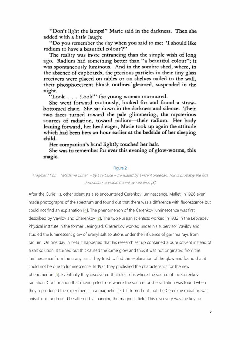
Figure 2
Fragment from “Madame Curie”- by Eve Curie – translated by Vincent Sheehan. This is probably the first
description of visible Cerenkov radiation [3].
After the Curie’s, other scientists also encountered Cerenkov luminescence. Mallet, in 1926 even
made photographs of the spectrum and found out that there was a difference with fluorescence but
could not find an explanation [4]. The phenomenon of the Cerenkov luminescence was first
described by Vavilov and Cherenkov [2]. The two Russian scientists worked in 1932 in the Lebvedev
Physical institute in the former Leningrad. Cherenkov worked under his supervisor Vavilov and
studied the luminescent glow of uranyl salt solutions under the influence of gamma rays from
radium. On one day in 1933 it happened that his research set up contained a pure solvent instead of
a salt solution. It turned out this caused the same glow and thus it was not originated from the
luminescence from the uranyl salt. They tried to find the explanation of the glow and found that it
could not be due to luminescence. In 1934 they published the characteristics for the new
phenomenon [5]. Eventually they discovered that electrons where the source of the Cerenkov
radiation. Confirmation that moving electrons where the source for the radiation was found when
they reproduced the experiments in a magnetic field. It turned out that the Cerenkov radiation was
anisotropic and could be altered by changing the magnetic field. This discovery was the key for

researchers Franck and Tamm to come up with the theory for the Cerenkov phenomenon [6]. They
explained the characteristics of the Cerenkov radiation and stated a formula to calculate the number
and angle of photons depending on the energy of the charged particle and the refractive index of
the medium. This is the so called Frank Tamm formula. In 1958 Cerenkov, Frank and Tamm received
the Nobel Prize for Physics for their discovery. A timeline on the history of Cerenkov luminescence
can be found in appendix A.
2.2 APPLICATIONS
The most prominent development following the discovery of Cerenkov radiation was the Cerenkov
Counter [2]. This is basically a large water tank with photomultiplier detectors to detect the photons.
The device is capable to detect high velocity charged particles like a Geiger Muller counter. The
advantage, however, is that it is way faster and in addition is able to determine the direction the
particle travels and its primary energy. In the following years Cerenkov radiation was mainly used in
particle physics. The light coming from high energy particles formed an ideal method of detecting
high energy nuclear interactions. This led to a lot of knowledge of neutrinos. It is also used in
neutrino astronomy like the detection or cosmic air showers [7]. This can be done with big size
Cerenkov counters as the SuperKamioKande, a 40 by 50 meter water basin covered by
photomultipliers in an underground cave in Japan.
The first appearance of Cerenkov radiation in medical biology in 1971 was the study into diagnosis of
eye tumours after the administration of Phosphorus 32 (32P). This 32P is incorporated preferentially in
dividing and thus malignant tissue. The idea was that the Cerenkov light originating in the vitreous
humour would be detected by the patient [8]. This idea was based on the discovery of cosmic rays
causing flashes in astronaut’s eyes during the early space missions.
Although Cerenkov in his Nobel prize speech mentioned that the usefulness of Cerenkov radiation
would extend rapidly in the future it was until 2009 where Robertson described a totally knew
biomedical application for the light phenomenon [1], [9]. He was the first one to perform optical
imaging based on Cerenkov luminescence derived from PET tracers in mice. He was hereby helped
by the high sensitivity camera systems that were developed for low light imaging as in fluorescence
and bioluminescence. Since then, Cerenkov luminescence imaging has quickly emerged as a
preclinical molecular imaging modality and a lot of new applications in clinical research were
developed based on CLI such as cancer imaging [10]–[13], therapy monitoring [14]–[16],
radionuclide detection [17], dose calibration for radiotherapy [18], [19] and fluorophore excitation
[20]–[22]. In the last 6 years a lot of knowledge is gained on the use of different radiotracers, and on
how to make the technique more sensitive. This led to the understanding that we have the

7
possession of a compact, high resolution molecular device which could have a lot of potential in the
medical clinic. Currently a lot of efforts are done to translate the applications from a preclinical
setting into applications that can be used in oncology. Cerenkov based Image guided surgery is one
of those prestigious ideas.
2.3 PRINCIPLES OF CERENKOV RADIATION
Cerenkov radiation or Cerenkov luminescence is light that arises when a charged particle moves
through a dielectric medium with a speed exceeding the speed of light 𝑐𝑐, in that particular medium.
The first thing that should be noticed is that particles are exceeding the speed of light. The concept
of particles exceeding the speed of light was already described independently by Oliver Heaviside
(1888) [23], Lord Kelvin (1901) [24] and Arnold Sommerfeld (1905) [25]. They all described how an
electromagnetic cone forms round the moving particle by the disturbance of the magnetic field.
Analogous to how Mach described the sonic boom, where particles exceed the speed of sound.
However, due to Einstein’s theory of relativity (1905) this earlier work was neglected for several
years until it was adopted by Franck and Tamm to explain the light found by Vavilov and Cerenkov.
It turned out that particles can indeed travel with a speed higher than the speed of sound.
However, this can only take place in a dielectric medium. A dielectric medium is a medium with a
high polarizability, optical transparency and has insulating properties. Lots of media are dielectric
such as water but also organic tissues.
The speed of light in vacuum is determined by the parameters permeability and permittivity. This is
the well-known constant 𝑐𝑐 (299 792 458 m/s). The wave velocity in a medium is dependent on the
polarizability of the materials in the medium. This is also called the phase velocity the higher the
polarizability the slower the velocity of light is in the material. The ratio between the speed of light in
vacuum and the phase velocity of light we call the refractive index. The refractive index thus
determines the speed of light in that particular material. In water where the refractive index is 1.33
(𝑛𝑛 = 1.33) the speed of light is only 𝑐𝑐/1.33 = 0.75 𝑐𝑐. This means that a particle can travel faster than
light in this medium without compromising the special theory of relativity.
Charged particles can travel statically through a medium. When this occurs in a polarizable medium
the molecules of that medium along the path of the charged particle are excited to higher states.
When these molecules relax back to their ground state these molecules emit some photons in the
form of electromagnetic waves. If the charged particle moves slower than the phase velocity 𝑛𝑛/𝑐𝑐
these electromagnetic waves do not interact with each other and extinguish slowly. However, if the
particle moves faster than the electromagnetic waves, the waves cross each other and add up at
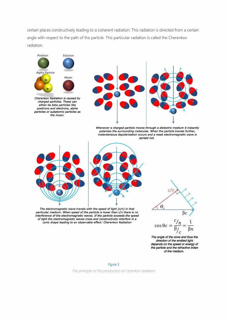
certain places constructively leading to a coherent radiation. This radiation is directed from a certain
angle with respect to the path of the particle. This particular radiation is called the Cherenkov
radiation.
Figure 3
The principle of the production of Cerenkov radiation.

9
2.3.1 WHEN DOES CERENKOV LIGHT OCCUR?
From the definition of Cerenkov radiation we know that there are three conditions that have to be
met. There will have to be charged particles. They have to travel in a dielectric medium. At last they
have to exceed the phase velocity. Charged particles may result from radioactive decay such as
positrons, β and α particles or as a result of internal conversions due to gamma or X-rays. A
dielectric medium is an insulating and optical transparent medium but most of all it means that the
molecules making up the material are polarizable. Water and many other liquids are dielectric and
thus so are organic tissues.
The last condition is the most difficult one. The speed of the particle has to exceed the phase
velocity of the medium. This thus depends on the kinetic energy of the particle and the refractive
index of the media. For moving objects we know the famous formula of the relativity theory by
Einstein, 𝐸𝐸 = 𝑚𝑚𝑐𝑐2. In developing its special relativity Einstein found for the kinetic energy of a
moving body the following formula:
𝑬𝑬𝒌𝒌 = 𝑴𝑴𝑴𝑴𝟐𝟐 � 𝟏𝟏𝒗𝒗𝟐𝟐
𝒄𝒄𝟐𝟐
− 𝟏𝟏� ( 1 )
With this formula the velocity of the particle can be calculated in terms of 𝑐𝑐, the speed of light when
the kinetic energy of the particle is known. Furthermore, the phase velocity can be calculated in
terms of 𝑐𝑐 by the following formula:
𝒗𝒗′ = 𝒄𝒄𝑵𝑵
( 2 )
This means that for a certain refractive index 𝑛𝑛, there is a threshold for the kinetic energy where the
particle will exceed the speed of light, and thus Cerenkov light arises. For a positron in water, which
has a refractive index of 1.33, this threshold is 263 KeV. However, if the refractive index increases the
threshold decreases. In figure 4 the threshold energy for Cerenkov is plotted against the refractive
index. For β particles like positrons and electrons, which have a very low mass these thresholds can
be easily overcome. α particles, however, have too much mass and therefor their energy threshold
is many times higher to obtain a speed higher than the phase velocity. In practice α particles will not
directly be the source of Cerenkov radiation.
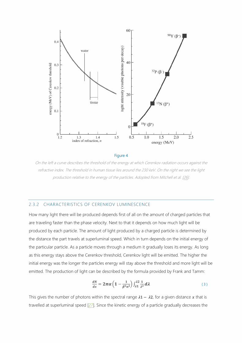
Figure 4
On the left a curve describes the threshold of the energy at which Cerenkov radiation occurs against the
refractive index. The threshold in human tissue lies around the 230 keV. On the right we see the light
production relative to the energy of the particles. Adopted from Mitchell et al. [26].
2.3.2 CHARACTERISTICS OF CERENKOV LUMINESCENCE
How many light there will be produced depends first of all on the amount of charged particles that
are traveling faster than the phase velocity. Next to that it depends on how much light will be
produced by each particle. The amount of light produced by a charged particle is determined by
the distance the part travels at superluminal speed. Which in turn depends on the initial energy of
the particular particle. As a particle moves through a medium it gradually loses its energy. As long
as this energy stays above the Cerenkov threshold, Cerenkov light will be emitted. The higher the
initial energy was the longer the particles energy will stay above the threshold and more light will be
emitted. The production of light can be described by the formula provided by Frank and Tamm:
𝒅𝒅𝑵𝑵𝒅𝒅𝒅𝒅
= 𝟐𝟐𝟐𝟐𝟐𝟐�𝟏𝟏 − 𝟏𝟏𝜷𝜷𝟐𝟐𝒏𝒏𝟐𝟐
� ∫ 𝟏𝟏𝝀𝝀𝟐𝟐𝒅𝒅𝝀𝝀𝝀𝝀𝟐𝟐
𝝀𝝀𝟏𝟏 ( 3 )
This gives the number of photons within the spectral range 𝜆𝜆1 − 𝜆𝜆2, for a given distance 𝑥𝑥 that is
travelled at superluminal speed [27]. Since the kinetic energy of a particle gradually decreases the

11
intensity of the produced light is directly proportional to the energy of the particle as can be seen in
figure 4 [26].
The energy of a particle depends on the principle of how this particle is originated. This can be done
through excitation of certain gamma or X-rays. In this way the energy and direction of the charged
particle is determined by the excitation beam. The direction of the particles and thus the emitted
light are also dependent on the direction of the excitation. Another possibility for having charged
particles is radioactive decay. In this case the particles are transmitted isotropically from a
radioactive source. The energy of the charged particles is dependent on this source. We take
Fluorine 18 (18F), a widely used positron emitter in nuclear medicine, as an example. 18F sends out
positrons with a yield of 97%. The energy of these positrons form a parabolic spectrum around 250
Kev with a maximum of 633 keV (Fig. 5). The Cerenkov threshold in water (𝑛𝑛 = 1.33) is 263 keV.
Therefor 47 % of the emitted positrons will travel at superluminal speeds and thus form Cerenkov
light. By using the Frank and Tamm formula we can calculate the amount of light that is produced
per travelled distance for a certain initial energy and a wavelength range. Mitchell et al calculated
that an endpoint positron of 633 keV will emit 16 photons per mm in the visible spectrum of 400-
800 nm [26]. The distance that this positron will travel at superluminal speed in water is 2.1 mm [28].
This means that a 18F derived endpoint positron in water produces 34 Photons. However, as we can
see from the energy spectrum we expect positrons with less energy than 633 keV and therefore
overall less photons than 34 will be produced per positron.
To determine the average production of photons per decay, Mitchell et al performed a Monte Carlo
simulation. A point source with an energy spectrum of positrons emitted by 18F was modelled in a
volume of water. Based on the Frank and Tamm formula the pathway of positrons travelling at
superluminal speeds was modelled. The distance from the origin had a root mean square (RMS) of
0.3 mm. Since the number of photons can be calculated from distance travelled at superluminal
speed they determined that for 18F an average of 1.4 photons are created per decay, in the visible
spectrum. If the refractive index is higher, the Cerenkov threshold is lower and more photons will be
produced. In biological tissue with a refractive index of 1.4 the photon production will be 2.4 per
decay. If we take another radioactive source with a different and an overall higher energy spectrum
also more photons per decay will be formed. Yttrium 90 (90Y) which has an endpoint energy of 2.23
MeV will produce 57 photons per decay and thus produces 40 times as much light as 18F (Fig. 4 and
Fig. 5). Evidently the travelled path at superluminal speed will also be longer. The RMS of travelled
distance at superluminal speed for Y90 is 2 mm.
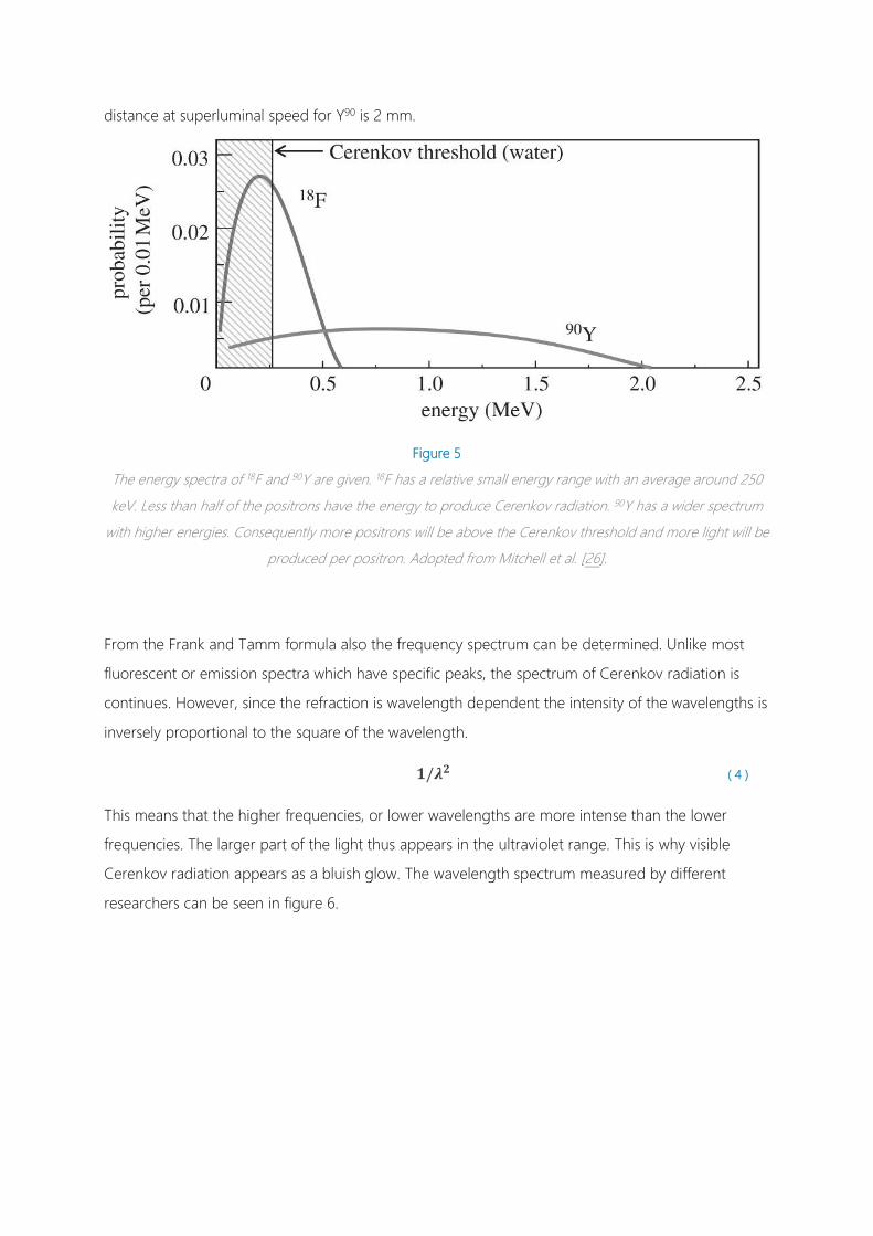
Figure 5
The energy spectra of 18F and 90Y are given. 18F has a relative small energy range with an average around 250
keV. Less than half of the positrons have the energy to produce Cerenkov radiation. 90Y has a wider spectrum
with higher energies. Consequently more positrons will be above the Cerenkov threshold and more light will be
produced per positron. Adopted from Mitchell et al. [26].
From the Frank and Tamm formula also the frequency spectrum can be determined. Unlike most
fluorescent or emission spectra which have specific peaks, the spectrum of Cerenkov radiation is
continues. However, since the refraction is wavelength dependent the intensity of the wavelengths is
inversely proportional to the square of the wavelength.
𝟏𝟏/𝝀𝝀𝟐𝟐 ( 4 )
This means that the higher frequencies, or lower wavelengths are more intense than the lower
frequencies. The larger part of the light thus appears in the ultraviolet range. This is why visible
Cerenkov radiation appears as a bluish glow. The wavelength spectrum measured by different
researchers can be seen in figure 6.

13
Figure 6
Different measurements on the wavelength of the Cerenkov induced luminescence. In all graphs we slightly see
the relation to the inverse square of the wavelength. Reproduced from [29]–[31]

3 CERENKOV LUMINESCENCE IMAGING USING CLINICALLY USED
RADIOTRACERS
3.1 CONCEPT OF CERENKOV LUMINESCENCE IMAGING
In 2009 Robertson et al. found a new scope for the Cerenkov effect. They discovered that Cerenkov
radiation also occurs with positron emitting radiotracers in biological tissue, but more importantly
that this radiation could be imaged optically. This resulted in a new molecular optical imaging
modality based on FDA (Food and Drug Administration) and EMA (European Medicines Agency)
approved positron emitting radiotracers with extensive possibilities. This technique is now known as
Cerenkov luminescence imaging. Since the first publication a lot of research has been done by
different groups scattered throughout the world. It started with in vitro and preclinical small animal
studies but in only a few years’ time this has led to numerous possible clinical and preclinical
applications. The overall conclusion of most publications is that the technique is at least ‘ feasible’
and more outspoken ‘very promising’.
The concept of Cerenkov Luminescence Imaging is to inject PET radiotracers into a human body or
an animal subject. These radiotracers tend to spread to specific tissues in a the body. The PET
tracers send out high energetic positrons which will produce Cerenkov luminescence in biological
tissue. When this takes place in a completely dark environment, the emitted photons can be
detected through the tissue by means of a high sensitivity super cooled CCD camera.
To bring a new imaging technique into clinical practice the first question is where it can be of added
value compared with currently used modalities. In this chapter we try to answer this question by
presenting an overview of the broad range of possible application different researchers have
explored over the past years.
3.2 POSSIBLE APPLICATIONS FOR CERENKOV.
In the last six years many applications have been suggested. These applications have different
scopes, different purpose and/or different methods. Concerning the scope you can use Cerenkov
on animals, patients or on specimens. Next to that the purpose to use Cerenkov radiation makes a
big difference. You can either use it for diagnostics, therapy monitoring, treatment response, image
guidance or as excitation for photo therapy. Lastly there are different methods of how Cerenkov
imaging can be performed for instance in vitro or ex vivo, planar or tomographic. It is important that
the choices that are made are matched with each other in order to come up with a successful
15
clinical application. Tomographic optical imaging in humans is for instance improbable due to
penetration properties of optical signals. For this project we focused on Cerenkov imaging in
humans that could assist in oncological surgery.
3.2.1 ANIMALS VS PATIENTS
There is a lot of difference in using Cerenkov imaging for animals or for patients. The most obvious
reason is that the for imaging patients there are a lot of regulations that do not apply to small
anmals because they are euthanized afterwards. This is reflected primarily in the amount of
radioactivity that can be administered. The administration doses for patients have strict regulations
that can be neglected in small animals. Especially in mice the dose weight ratio can become very
high which will result in a dose per kilogram bodyweight that is over 100 times higher than is used in
human. Next to that the we are measuring light as a signal. Light has a very poor ability to penetrate
through biological tissue. This will make the technique feasible for imaging small animals that lack
thick layers of tissue. For imaging in a larger species such as humans, detecting light is more difficult
and imaging of deeper structures can only be done invasively. At last, there is the available imaging
system. For imaging mice, the commercially available IVIS (In Vitro Imaging System) can be used
(Fig. 7). This is a very sensitive precisely tuned and tailored system to perform low light imaging on
mice. The mice can be sedated and be imaged five at a time in a light tight cabinet. For patients,
such a device is not available and other solutions have to be found. Problems that arise here are to
obtain a light tight system that is as sensitive as the IVIS system keeping the size and the
convenience of the patient in mind.
3.2.2 OBJECTIVES
Since the discovery of CLI it is clear that it is a promising new modality for molecular imaging with
the use of PET tracers and as an additional advantage could image β- radiation or electron emission.
It would especially be suitable for preclinical mouse studies. This was independently stated by the
pioneers of Cerenkov Imaging, [1], [32], [33]. Hu et al. even explored the options for 3 dimensional
Cerenkov imaging or Cerenkov luminescence tomography [34].
Besides the straightforward applications as in vivo tumour imaging, treatment response and therapy
monitoring that are also used in PET imaging, there are numerous other applications suggested or
explored such as: In vitro assays [33], plant studies [33], imaging of pure β min emitters [30],
Reporter gene expression [30], source depth measurements [30], microfluidic chip measurements
[35], Imaging of α emitting radionuclides [36], imaging Cerenkov radiation excited by external
beam radiation [19], excitation of quantum dots or other luminescent material by CR for diagnostic

or therapeutic purposes[21], [22], [30], negative contrast imaging[37],selective bandwidth quenching
of the CR spectrum[17], [38] and CR imaging of positron distribution in proton therapy[18].
Figure 7
The in vivo imaging system which is designed especially for optical imaging with low light levels in small
animals. It consists of a light tight cabinet with a high sensitivity super cooled CCD camera with different lenses,
band filters and special lights to excite fuorophores. On our case we do not use the lights. Reproduced from
www.perkinelmer.com.
In 2010 Ruggiero et al. were the first to mention that optical imaging methods have to be translated
into the clinic so that endoscopy and surgery could benefit from it [39]. Shortly after that, from the
same group of the Memorial Sloan Kettering hospital, Holland et al, published a paper on
intraoperative Cerenkov luminescence imaging [12]. He performed intraoperative CLI on mice with
Zirconium 89 (89Zr) DFO-trastuzumab. The data he published really captures the imagination of the
application(Fig. 8). However, it was performed on mice and not on a clinical scale. Nevertheless, he
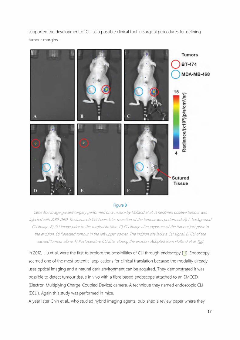
17
supported the development of CLI as a possible clinical tool in surgical procedures for defining
tumour margins.
Figure 8
Cerenkov image guided surgery performed on a mouse by Holland et al. A her2/neu positive tumour was
injected with Zr89-DFO-Trastuzumab 144 hours later resection of the tumour was performed. A) A background
CLI image. B) CLI image prior to the surgical incision. C) CLI image after exposure of the tumour just prior to
the excision. D) Resected tumour in the left upper corner. The incision site lacks a CLI signal. E) CLI of the
excised tumour alone. F) Postoperative CLI after closing the excision. Adopted from Holland et al. [12]
In 2012, Liu et al. were the first to explore the possibilities of CLI through endoscopy [11]. Endoscopy
seemed one of the most potential applications for clinical translation because the modality already
uses optical imaging and a natural dark environment can be acquired. They demonstrated it was
possible to detect tumour tissue in vivo with a fibre based endoscope attached to an EMCCD
(Electron Multiplying Charge-Coupled Device) camera. A technique they named endoscopic CLI
(ECLI). Again this study was performed in mice.
A year later Chin et al., who studied hybrid imaging agents, published a review paper where they

compared CLI to fluorescence [40]. In this review he pointed out what the current weaknesses for
CLI where namely ; low light, ambient light distortion, low penetration power and the necessary
radioactivity. Nonetheless he stated that it is a very exciting research line and that these limitations
could be overcome by technical developments.
In 2013 the first CLI on humans was performed. Spinelli et al. detected light emitted from the thyroid
of a patients treated for hyperthyroidism with Iodine-131(131I) [41].This was the first proof that CLI
was actually possible in patients. (Fig. 9) This result suggested the application of monitoring
radiation dose of therapy with β emitters in superficial organs. This would especially be relevant for
β- emitters since there is currently no efficient way of imaging them.
In that same year Thorek et al. also performed CLI in humans [42]. He had performed a pilot study
on four patients and they showed that they were able to image a positive axillary node in a patient
with lymphoma after injection of 18F-FDG. With this result they demonstrated it was feasible to
detect tumours with CLI using diagnostic doses of 18F-FDG. They also stated that for establishing the
value of CLI for clinical use, they required larger studies with possible more sensitive equipment and
higher energy positrons. From the article it is not really clear how they exactly obtained their results.
This is also questioned in a response to this article made by Spinelli and Boschi [43]. Despite the fact
that a lot of the criticism could be refuted, the results of Thorek is difficult to explain next to the
other published data concerning CLI. Even today a reproduction of Thoreks work has not been
published.
In 2014, Jarvis et al. published its results on the visualization of the surface dose due to radiation
therapy [19]. By use of CLI he was able to image the surface dose on human subjects in real time.
They proposed that Cerenkov video imaging could detect errors in everyday clinic and therefor
improve the safety and quality of radiation therapy.
The latest published study performed in humans is a feasibility study for the ECLI system for
detecting gastro-intestinal disease. Hu et al. performed endoscopic CLI on four patients after 18F-
FDG administration [44]. They found elevated signals in cancerous tissue compared with normal
tissue. This result will make the application of CLI for endoscopic diagnostic procedures very
feasible.

19
Figure 9
Cerenkov imaging that is performed on humans. In the upper left corner we see a patient with who is treated
with 131I for hyperthyroidism. 550 MBq was administered and after 24 hours a 2 minute acquisition with a
EMCCD camera was made. A clear elevated intensity can be seen at the position of the thyroid gland. Adopted
from [41]. On the upper right we see a malignant lymph node in the axilla that is imaged with an ICCD camera.
470 MBq of 18F-FDG was administered and after 68 minutes a 5 minute acquisition was made. Image B and D
show the left axilla which shows elevated intensity corresponding to the PET examination (E). Adopted from
[42]. In the lower left corner we see the results of an endoscopic approach of CLI. With a fiberscope coupled to
an EMCCD camera malignant tissue (A and C) is compared to benign tissue (B and D). For this study this

patient was administered with 9.25 MBq/kg 18F-FDG was administered. Adopted from [44]. In the lower right
corner we see an image from a study from Jarvis et al. He imaged the dose on the surface of a breast that is
radiated with an external beam. This high energetic radiation causes Cerenkov radiation in human tissue that
can be real time monitored with an EMCCD camera during the treatment. Adopted from [19]
In the most recent years Cerenkov radiation has been explored for therapeutic purposes. This was
initiated by the work to overcome the problems of the penetrability of Cerenkov light. It was
demonstrated that fluorescent probes as small molecules and quantum dots could be excited by
Cerenkov radiation [45]. This meant that the spectrum of Cerenkov radiations that peaks in the blue
and green wavelengths could be changed to narrow band high penetrable wavelengths without
compromising the tissue specificity of the used radioisotope.
Ran et al. were the first to describe the concept of Cerenkov radiation as a tissue specific light
source [21]. He used Cerenkov radiation derived from administered 18F-FDG as photo activation of
luciferin to have activation at specific malignant sites deep in vivo where external photo activation
was not possible.
In a recent review published by Grimm, the results of the group from Achelifu was discussed [22].
They studied the activation of titanium dioxide nanophotosensitizers (NPS) by Copper-64 (64Cu).
When he injected both in fibrosarcoma tumours in mice, the disease showed a complete regression
in 30 days. They repeated this with a slightly different approach by injecting the NPS and 18F-FDG
intravenously. Also this study showed good result. Again there is a remark that this work was
performed on mice and that NPS as were used here have a long way to go before they can be used
in clinical practice.
From the literature it can be concluded that CLI has a large potential. Many researchers describe the
possible uses in clinical practice. The current results however, are very poor and as with all optical
imaging the translation from small animals to life-size humans is difficult due to the attenuation of
light by tissue. To make a successful start into clinical translation more easily adaptable applications
should be developed first. Such small steps are for instance made with the ECLI. It might not have a
large impact on clinical relevance but foremost it is likely to succeed since an optical guided
procedure and system are already implemented in endoscopic examinations and it makes use of the
naturally dark environment in the colon. For assistance in oncological surgery can be thought of
margin detection as the principle application. For this only small specimens have to be imaged and
there is no need to look in deeper layers of the tissue.
3.3 RADIOTRACERS

21
As it appears from the literature there are a lot of properties that make CLI very difficult. The
biggest challenge perhaps is that the Cerenkov light is produced in very low quantities, resulting in a
weak signal. It should be noticed that a lot of research is currently performed on enhancing the CLI
signal. Next to that this weak signal has to stand out against the background. A problem we also
encounter with other nuclear modalities and with fluorescence optical imaging. The amount of light
and also the signal to background ratio is determined by the type of radiotracer that will be used.
Today there are a lot of different radiotracers available for different purposes. To have an overview
of what radiotracers are suited for CLI and which one is the best option for a specific purpose this
paragraph gives an overview of the clinically used radiotracers and their most important properties
for CLI.
It has been made clear that Cerenkov radiation arises when radioactive decay occurs in water or
biological tissue. There are a lot of radionuclides used in nuclear medicine, over 40 different
isotopes. But there are a handful of properties that make these isotopes suitable for Cerenkov
imaging.
1. The first and most important factor is that the radioisotope has to emit high velocity
charged particles. With high velocity we mean they have to possess a certain energy that
enables the particle to move faster than the phase velocity or medium specific speed of
light. In general these include all isotopes that emit either positrons or electrons of sufficient
energy. α particles typically are too heavy to be able to reach speeds like that. However,
certain isotopes which initially decay into α particles or γ rays might produce daughters that
emit high energy β particles. However, the forming of the daughters might cause a delay in
obtaining a signal. This means that radioactive isotopes that produce Cerenkov radiation
are the ones that decay trough β particles or produce daughters that will decay by β
emission.
2. The second important factor is that it has a sufficient amount of yield and energy. The
amount of light that is produced by Cerenkov radiation is relatively low and to make a light
source visible, especially within a tissue, an intended number of photons is required. The
amount of photons that are produced depend mainly on the number of charged particles
that are emitted. This can be determined by the activity and the yield. Furthermore the
energy of the charged particles is important. The higher the energy the more photons it will
produce before it drops under the Cerenkov threshold. For positrons in biological tissue
with a refractive index of 1.4 this threshold is 230 keV. Therefor isotopes with a high yield of
β emissions and a high initial energy of those β particles are particularly suitable for
Cerenkov imaging.
3. The half-life of an isotope is also important for imaging purposes. Since we want to image
light that is emitted by radioactive decay the signal is directly associated to the activity of the
radioactive source. We have to make sure that there is enough activity at the right site in a
human or animal body or even in a specimen at the time of the imaging. The half-life of the
isotope should not be too low in order to keep the activity on an intended level for imaging
and to give the pharmacokinetics the time to reach the targeted parts. Next to that you also
want a half-life that is not too long to make sure the radioactivity is cleared from a subject
within a reasonable time. On the contrary, there are some circumstances a longer half-life
could be beneficial. If the radioisotope probes can stay at its target for a prolonged time the
majority of the activity, that is not specifically bound, will leave the body by excretion. This
could reduce the total activity in the whole body while maintaining a high activity at the
targets of interest. For instance in intraoperative Cerenkov imaging this could reduce the
radiation dose to the surgeons. Due to this diversity in applications we accept a broad
range of half-lives.
4. The radioisotope that you want to image should have a clinical value. This means that the
information of the distribution of the isotope through the body or specimen gives you
relevant information. The isotope therefor has to possess some properties to bind to certain
elements or structures that are interesting to visualize. These properties can either be part of
the isotope itself or come from a molecular labelling structure it can bind or chelate to.
Radiotracers suitable for CLI are thus the ones with specific binding or distribution capacities.
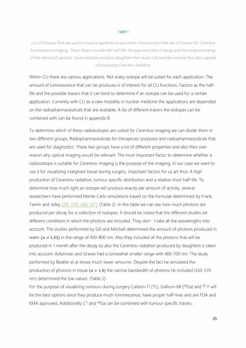
5. The last important property which is one of the important benefits of CLI is that the
radiotracers are FDA or EMA approved and already used in the clinic. Based on these
properties a list of isotopes is composed that seem to be suitable for Cerenkov imaging
(Table 1).
23

25
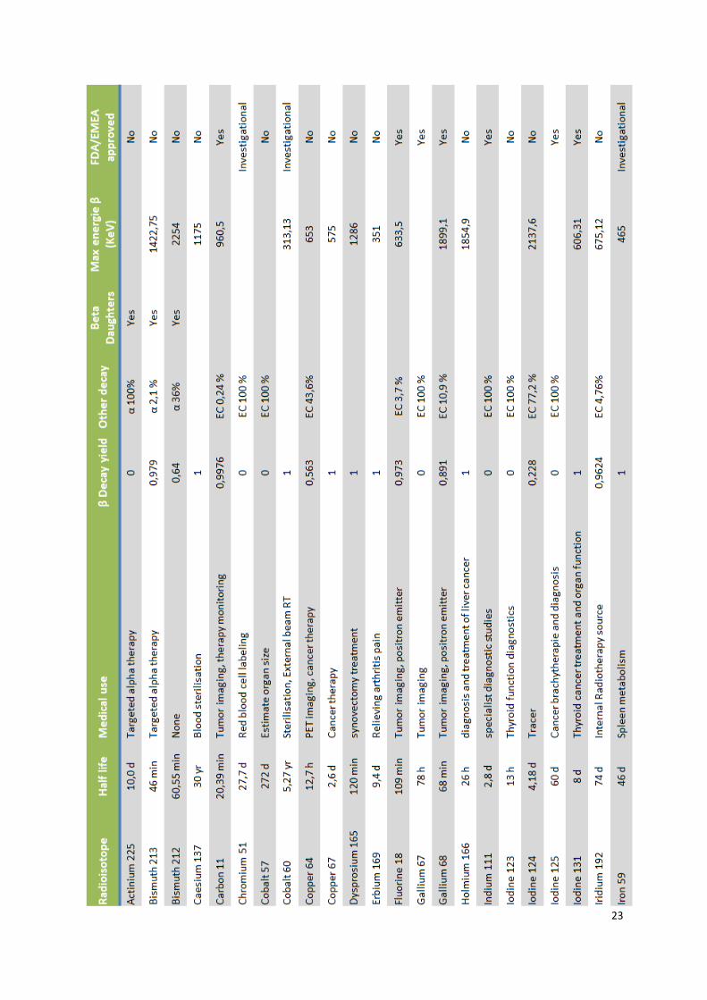
Table 1
List of isotopes that are used in medical applications and there characteristics that are of interest for Cerenkov
luminescence imaging. These factors include the half-life, the type and yield of decay and the endpoint energy
of the derived β particles. Some isotopes produce daughters that result in β particles and are thus also capable
of producing Cerenkov radiation.
Within CLI there are various applications. Not every isotope will be suited for each application. The
amount of luminescence that can be produces is of interest for all CLI functions. Factors as the half-
life and the possible tracers that it can bind to determine if an isotope can be used for a certain
application. Currently with CLI as a new modality in nuclear medicine the applications are depended
on the radiopharmaceuticals that are available. A list of different tracers the isotopes can be
combined with can be found in appendix B.
To determine which of these radioisotopes are suited for Cerenkov imaging we can divide them in
two different groups. Radiopharmaceuticals for therapeutic purposes and radiopharmaceuticals that
are used for diagnostics. These two groups have a lot of different properties and also their own
reason why optical imaging would be relevant. The most important factor to determine whether a
radioisotope is suitable for Cerenkov imaging is the purpose of the imaging. In our case we want to
use it for visualizing malignant tissue during surgery. Important factors for us art thus: A high
production of Cerenkov radiation, tumour specific distribution and a relative short half-life. To
determine how much light an isotope will produce exactly per amount of activity, several
researchers have performed Monte Carlo simulations based on the formulas determined by Frank,
Tamm and Jelley [26], [36], [46], [47]. (Table 2). In this table we can see how much photons are
produced per decay for a collection of isotopes. It should be noted that the different studies set
different conditions in which the photons are included. They don’t take all the wavelengths into
account. The studies performed by Gill and Mitchell determined the amount of photons produced in
water (𝑛𝑛 = 1.33) in the range of 400-800 nm. Also they included all the photons that will be
produced in 1 month after the decay so also the Cerenkov radiation produced by daughters is taken
into account. Ackerman and Graves had a somewhat smaller range with 400-700 nm. The study
performed by Beattie et al shows much lower amounts. Despite the fact he simulated the
production of photons in tissue (𝑛𝑛 = 1.4) the narrow bandwidth of photons he included (550-570
nm) determined the low values. (Table 2)
For the purpose of visualizing tumours during surgery Carbon-11 (11C), Gallium-68 (68Ga) and 90 Y will
be the best options since they produce much luminescence, have proper half-lives and are FDA and
EMA approved. Additionally C11 and 68Ga can be combined with tumour specific tracers.

Table 2
This table gives an overview of four studies that are conducted to determine the amount of Cerenkov radiation
that is produced per decay. This is based on performed Monte Carlo simulations. The different studies used a
different range for the wavelength and are therefore not comparable with each other. However, the studies per

27
se give a good estimation on the relative difference in light production between different isotopes. The study
performed by Ackerman et al. was done to determine the amount of light produced by the intrinsic isotope
and the total through all the daughters. This number is given in brackets.[26], [36], [46], [47]

4 IMAGE GUIDED SURGERY
4.1 DIFFICULTIES IN SURGICAL ONCOLOGY
One of the biggest challenges in surgical oncology is often to make sure all of the malignant tissue
is removed without compromising functional and cosmetic outcomes. To achieve this, a surgeon
should be very well aware where the primary tumour and possible metastasis are located within the
body. Besides the location of the tumour, its location with respect to critical organs is very
important. The next step is to make sure the surgeon exactly knows what tissue belongs to the
tumour and what not. In other words he has to make a distinction between malignant and benign
tissue.
Over the past decades several techniques are developed for locating a tumour. In most cases this is
done based on imaging that took place days or weeks before the surgery. This can either be CT,
MRI, PET-CT or Ultrasound imaging. With these modalities the location and often the spatial
orientation can be recovered. Based on these images and the anatomical knowledge of the surgeon
a plan is made prior to the surgery. The difficulty with this method is that the patient’s position
between imaging and surgery can be changed and additionally the position of the tumour can
change during surgery. Furthermore the time between them could have caused proliferation or
shrinkage of the tumour. Several techniques are currently performed to improve this method. One
of the most recent applications is surgical navigation. This tracks and registers the position of the
patient and the tools of the surgeon and displays it on an imaging based model. However, in cases
as breast and rectal cancer the organs are very mobile during surgery and lack the proximity of rigid
anatomical landmarks which are important for navigation and intra-operative guidance. There are
numerous ways to solve this including; intraoperative ultrasound guided resection, the placement of
guide wires or markers, the use of dyes, cryoprobe assisted localization or the use of injected
radiopharmaceuticals [40], [48]–[50]. With the help of radiography and or gamma probes the exact
location of the tumour can be determined during the surgery.
This means that the first step, localizing a tumour, is pretty well solved. However, all these
techniques do not solve the second step of discriminating tumour tissue from healthy tissue. To do
this surgeons still depend on their visual and tactile input. For some tumours this is a difficult task
since they have almost the same visual and textural properties as the surrounding healthy tissue.
Also in patients that have recurrent disease or who underwent extensive chemo-radiotherapy,
determining the borders of the tumour is even more difficult due to a disturbed anatomy and

29
fibroses caused by prior surgery or radiation. It follows that resection in these cases is hampered
and will impede optimal tumour resection.
4.2 POSITIVE SURGICAL MARGINS (PSM)
A non-clean resection means that there are positive surgical margins. In the literature researchers
have reported positive margin rates of 20-40% in breast conserving treatment of primary breast
tumours [48], 16-27% in radical prostatectomy [51], [52], and up to 28 % in rectal cancer [53]. It
should be noted that these are not the current numbers representative for the NKI-AvL (Netherlands
Cancer Institute – Antoni van Leeuwenhoek) , but findings in other centres in the Netherlands and
other western countries. PSMs are a typical risk factor for local recurrence. Positive margins in
patients who received breast conserving surgery will give a fivefold increased risk of local recurrence
[54]. In prostatectomy PSM will lead to a fivefold increased risk of additional treatment [51]. Besides
the additional treatment in the form of surgery or radiation therapy, PSMs will lead to uncertainty
and anxiety for the patient. Next to that the additional treatment comes with extra costs, risks and
more discomfort for the patient. It should be noted that the assessment of PSMs is not an exact
science and therefore not always properly diagnosed. Improper diagnosis will results in an even
higher risk for local recurrence [55]–[57], and hence a worsened patient outcome. This provides
even more reason to prevent positive surgical margins.
One of the approaches to obtain clean margins is to do intraoperative margin assessment. Several
techniques have been explored over the last decades such as: Intraoperative Specimen
Radiography, frozen section analysis and intraoperative touch preparation cytology (imprint
cytology )[58]–[60]. Of these only the latter showed promising results but is not widely implemented
because it is not applicable to most of the tumours and requires on site pathology personnel.
Another approach is to develop a technique that enables the surgeon to distinguish tumour tissue
from healthy tissue even when the visual and textural appearance cannot be distinguished. We can
already do this with different types of imaging like MRI or PET-CT. In this case we need an imaging
device that is very tumour specific and next to that has a very high sensitivity and resolution to
detect small tumour manifestations. For practical reasons it also has to be easy to handle, easily
implementable and fast. And with fast we mean at least near real time. The one technique that
seems very suitable for this kind of image guidance is optical imaging.

Figure 10
The new hallmarks of cancer. The properties that define malignancy. They consist of the 6 originally hallmarks
proposed in 2000 completed with four new processes that characterize malignant tissue. Adopted from [63]
4.3 OPTICAL IMAGING
Optical imaging systems have the advantage of being free of ionizing radiation, being easy to
handle, having fast acquisitions and a high resolution. Next to that they are relatively inexpensive
and can be easily implemented in a surgery setting. Real time technologies really puts the images
directly in the hands of the surgeon. The big question is how we can distinguish tumour tissue. The
answer to this question can be found in the hallmarks of cancer: 10 different properties that define
malignancy. (Fig. 10) These properties can be used to make a distinction between benign and
malignant tissue.
There are different forms of optical imaging that can be used for optical imaging. Autofluorescence
is the intrinsic fluorescence of tissue that is excited by a certain wavelength of light. An advantage is
that no exogenous agents have to be administered. It is shown that they found robust correlations
for elevated red fluorescence and decreased green fluorescence in tumour tissue in the oral cavity
[61]. However, the technique did not show an advantage over the naked eye and furthermore the
specificity of the detection remains uncertain because it is not clear what the exact contribution of
the individual components are [62].
31
In conventional fluorescence they use probes that emit between 400-600 nm that will give high
levels of nonspecific background in tissue. Furthermore they have little optical penetration and a lot
of absorption by haemoglobins. Since optical imaging is all about the signal to background ratio,
and for this purpose tumour to background ratio, conventional fluorescence in not a good choice
for image guided surgery.
Near infrared (NIR) fluorescence was a crucial step in optical imaging and especially for imaging in
vivo. The optical imaging window where the least absorption and scattering takes place in tissue lies
between 700 and 900 nm. (Fig. 11) Probes with these wavelengths thus have a better penetration,
less scattering and less autofluorescence and therefor provide a better signal to background ratio.
There are different approaches to form suitable fluorophores for NIR fluorescence [62]:
• Non targeted fluorophores as fluorescein and indo cyanine green (ICG) which have excellent
fluorescent properties but do not have the ability to bind to a specific tissue.
• Non-targeted activatable fluorophores. These are non-specific markers that are delivered in
a quenched state. Due to cleavage of certain enzymes they can be activated to make them
more specific to tissues where the intended enzyme is situated. However, this has not led to
tumour specific agents yet.
• Targeted organic fluorophores are NIR fluorescent agents that have the ability to provide
molecularly specific detection. The agents are foremost conjugated to specific target ligands
or monoclonal antibodies. Different types of fluorophores like Cy 5.5, Alexa Fluor and
IRdye800CW are targeted to epidermal growth factor (EGF), vascular endothelial growth
factor (VEGF) or her2/neu receptors. These agents show excellent signal to background ratio
and this can even be increased by using specific quenching.
• Quantum dot nanoparticles are small inorganic crystals. They can provide high signal
intensities and can be designed to peak at a certain wavelength. Furthermore they can be
targeted to multiple biomarkers. Unfortunately the quantum dot nanoparticles show a high
level of toxicity that forms a large obstacle for their way into the clinic.
Techniques like fluorescence seem very suitable for tumour localization and intraoperative margin
assessment. Although the recent years has seen an increase in the number of commercially available
fluorophores, translation towards the clinical setting is still very limited. Their appearance in clinical
practice is hampered by lacking FDA or EMA approval and limited standardization of production,
imaging and quality control [64].

Figure 11
In this graph we can see the different absorption coefficients in human tissue against the wavelength. The
region between 700 and 900 nm has we see a lower absorption by bound and unbound haemoglobin and
water. This region is also known as the optical window. In light blue we see the spectrum of Cerenkov
luminescence which shows a very low yield in this particular window. Reproduced from [65]
4.4 OPTICAL AND MOLECULAR IMAGING COMBINED.
The question that remains is on how we will be able to detect malignant cells by optical imaging. A
good example for tumour specific imaging can be found in nuclear imaging and PET in particular.
They are capable of detecting malignancies using highly tumour-specific radioactive tracers that are
readily available for clinical use. The mainstay tracer for oncology is 18F-FDG, which makes use of the
increased metabolism due to the limitless replicative potential. It is used to localise lesions, monitor
disease burden and therapy efficacy. Unfortunately, the technology used for the detection of
radioactivity is less suitable for intraoperative use because it lacks the resolution, the speed and the
ease of use we need for image guidance during surgery.
CLI provides us with the means of combining optical imaging with molecular imaging through
clinical available radiopharmaceuticals. It actually combines the best of both worlds. From the optical
imaging point of view we have the advantage that it is a sensitive technique with a high resolution.
The optical devices are relatively inexpensive, easy to operate and can be easily implemented into
clinical practice due to their small profile. Furthermore they are capable of fast acquisitions and able
to provide real time or near real time imaging data.
The radioactive molecular imaging probes provide us with a wide range of clinically available and

33
approved probes. These radiopharmaceuticals are widely used and produced on large scale and
therefore relatively inexpensive. This means that no large costly studies into pharmacokinetics and
toxicology are required and there can be a rapid translation into clinical practices. Also, performed
studies have proven that CLI can provide a quantative measure and that it shows good correlation
with PET studies [1], [10], [39], [66].
Figure 12
This graph shows the emission intensity of the different wavelengths of Cerenkov luminescence compared with
fluorescent and bioluminescent agents. We clearly see that most of the Cerenkov signal is located in the
ultraviolet region. Additionally the intensity peak is a factor 1000 lower than the other agents. Adopted from
[40].
These characteristics make CLI very promising as a new technique for image guided surgery.
However, there are also some limitations that have to be overcome before CLI can be actually
applied in the clinic. First of all, the signal derived from the Cerenkov effect is very low, more than
three orders of magnitude less than luminescent markers. (Fig. 12) This results in two additional
challenges. First of all the signal is so low that it can be overshadowed by any glimmer of ambient
light. This requires that images have to be made in total darkness. For in vivo imaging in humans
this will not be easy and especially in a surgical setting this will be very difficult to accomplish.
Secondly, this means that to obtain a sufficient signal, lots of radiotracer should be administered. Liu
et al. calculated that for her endoscopic system an amount of 2.1 GBq (giga Becquerel) should be
administered to obtain detectable concentrations in a small head and neck tumour [11]. Since the
administration preferably has to take place several hours before the surgery, decay determines that

the administered dose should be even higher. This will lead to very high doses for the patients but
also for the OR personnel who have to follow much stricter rules for exposure.
The low signal intensity will become even a bigger problem when performing imaging in vivo. This is
caused by the nature of the spectrum. The yield is proportional to the inverse square of the
wavelength. (Eq. 4 ) As a result the spectrum peaks at 180 nm with the majority of the light in the
ultraviolet region and only a fraction of the light in the optical imaging window (700-900 nm).
Thus, with performing CLI in practice we face the challenge of having a low signal of which only a
small portion is usefull when used in vivo.
35
5 EMCCD CAMERAS
In order to make Cerenkov radiation visible we need a very sensitive camera which provides a very
high signal to noise ratio in a very low light environment. For this purpose we use an EMCCD
camera. EMCCD stands for electron multiplying charge-coupled device. It is an innovative design for
amplifying low light signals above the read noise floor of already sensitive CCD sensors without
compromising the quantum efficiency. Together with low costs and a high resolution this makes it
better candidate than other high sensitive cameras as for instance the intensified CCD.
The low light capabilities of EMCCD are primarily of use in astronomy and biomedical research. In
astronomy it is used to look at faint stars. Biomedical applications are photon counting and different
types of spectroscopy among others. More recently EMCCDs have broken into the field of
fluorescence microscopy and small animal imaging.
A CCD chip is a piece of technique that is extensively used in digital imaging. It enables the shift of a
charge to different areas of a chip for further processing. For instance, the conversion from charge
to digital values. The chip consists of two parts; an imaging part and a storage part. The upper
surface of the imaging part consists of a silicon photoactive region. Here incident photons are
transformed into photoelectrons. Under this layer each pixel of the chip is represented by a
capacitor well. Often this is a metal oxide semiconductor (MOS) capacitor. It stores and accumulates
charge proportional to the amount of incident photons during an acquisition.
The storing part consists of the same amount of capacitor wells as the imaging part. After an
exposure the charges of each capacitor well are shifted to the storing area. At this time the image
can be read out one line at the time and each pixel is converted from an analogous to a digital
signal. (Fig. 13) At the same time of the readout the imaging part can start a new exposure.

Figure 13
Working principle of a CCD chip. On the image section the photons are collected during the exposure time.
During the readout the charge in the capacitor wells which represent the pixels are shifted towards the store
section. From the store section they are read out per line and then per pixel converted to a digital signal.
Adopted from www.andor.com
In electron multiplying an additional gain is built in between the readout and the conversion to a
digital signal. This is done by a technique called the electron avalanche effect. This gain can be set
digitally and is capable of multiplying the charge by a thousand. The exact placement of this gain
results in the suppressing of certain noise factors leading to a higher signal to noise ratio [67].
5.1 NOISE SOURCES
With low light imaging it comes all down to signal to noise ratio. When imaging something it is the
goal to elevate the signal above the noise floor. There are different types of noise that have different
natures and contribute at different moments in the process (Fig. 14). For an EMCCD camera we have
the following types of noise[68]:
• Shot Noise (𝑵𝑵𝒔𝒔𝒔𝒔𝒔𝒔𝒔𝒔): This is a property of the quantum nature of light. It appears due to
statistical fluctuation of the number of photons that are emitted by the source. It can be
seen as the natural variation in the signal and this cannot be removed.

37
• Dark Current (𝑵𝑵𝒅𝒅𝒄𝒄): Is caused by thermally generated electrons in the photoactive part of
the CCD chip. This current also has its own stochastic variance known as the dark noise. The
contribution of dark current can be greatly reduced by lowering the temperature of the
chip to temperatures of minus 80 degrees Celsius. For these low temperatures the dark
current drops from 300 electrons per second per pixel at 20 degrees to lower than 0.001
electrons per second per pixel at minus 80 degrees.
• Readout Noise(𝑵𝑵𝒓𝒓): Is the noise that is generated by the electronic circuitry that converts
the charges to a digital signal. The readout noise has different contributors as the reset
noise, output amplifier noise, excess noise, quantization noise and clock induced charge. It
cannot be eliminated but the different contributors can be suppressed due to sophisticated
designs. Within an EMCCD chip we can divide the different contributors by noise generated
before reaching the gain amplifier as charge transfer noise (𝑁𝑁𝑐𝑐𝑡𝑡) and the remaining readout
noise (𝑁𝑁𝑟𝑟0).
• Total noise (𝑵𝑵𝒔𝒔𝒔𝒔𝒔𝒔): The total noise that is generated by an EMCCD is thus:
𝑵𝑵𝒔𝒔𝒔𝒔𝒔𝒔 = (𝑵𝑵𝒔𝒔𝒔𝒔𝒔𝒔𝟐𝟐 + 𝑵𝑵𝒅𝒅𝒄𝒄
𝟐𝟐 + 𝑵𝑵𝒓𝒓𝟐𝟐)𝟏𝟏/𝟐𝟐 ( 5 )
The shot noise and the dark current are both dependent on the integration time of the
acquisition. Therefor we can group them as 𝑁𝑁𝜏𝜏. Furthermore the charge transfer part of the
readout noise depends on the electron multiplying gain. This gives us the following total
noise:
𝑵𝑵𝒔𝒔𝒔𝒔𝒔𝒔 = (𝑵𝑵𝝉𝝉𝟐𝟐 + 𝑵𝑵𝒓𝒓
𝟐𝟐)𝟏𝟏/𝟐𝟐 ( 6 )
𝑾𝑾𝑾𝑾𝒔𝒔𝒔𝒔: 𝑵𝑵𝒓𝒓 = [𝑵𝑵𝒓𝒓𝒓𝒓𝟐𝟐 + (𝑮𝑮 × 𝑵𝑵𝒄𝒄𝒔𝒔)𝟐𝟐]𝟏𝟏/𝟐𝟐 ( 7 )

Figure 14
Here we see a schematic of an EMCCD camera. When the signal is collected through the lens of the camera
the signal only contains shot noise. With every part of the signal processing in the CCD chip the signal is
adjusted or noise is added. In the first step the signal is multiplied with the quantum efficiency (QE) of the CCD
at the same time dark current is added. When the pixels are read out the charge transfer noise is added. When
the EM-gain is applied the signal will be amplified at the cost of some more noise. Eventually when the signal
from the CCD chip is converted to digits output noise is generated.
5.2 SIGNAL TO NOISE RATIO
If we want to image very low light intensities we besides a sensitive system a system with a high
discriminative power of the signal. This is indicated with the signal to noise ratio:
𝑺𝑺𝑵𝑵𝑺𝑺 = 𝑺𝑺𝑾𝑾𝑺𝑺𝒏𝒏𝑺𝑺𝑺𝑺𝑵𝑵𝒔𝒔𝑾𝑾𝒔𝒔𝑵𝑵
( 8 )
We already know how the noise of an EMCCD system is constructed. However, also the signal
depends on the integration time and the electron multiplying gain. This results in the following
signal to noise ratio:
𝑺𝑺𝑵𝑵𝑺𝑺 = 𝑮𝑮×𝑺𝑺×𝝉𝝉(𝑵𝑵𝒔𝒔𝟐𝟐+𝑵𝑵𝒓𝒓𝟐𝟐)𝟏𝟏/𝟐𝟐 ( 9 )
Since we know from equation (7) that only a part of the noise is affected by the gain G, we can see
that increasing the gain higher than unity will result in a higher signal to noise ratio. In addition,
activating the gain will also result in excess noise produced by the electron multiplying procedure.
Thus the signal to noise ratio will only benefit when the amount of remaining readout noise is higher
than the noise due to the gain. Furthermore, as the charge packages begin to grow above 100
thousands of photons per pixel a problem arises with the charge transfer efficiency. Small amounts

39
of charges are left behind during amplification eventually leading to horizontal artefacts in the
image. The EMCCD camera will therefor only be beneficial for signals that are higher than the clock
induced charge and at the same time is not high enough to cause problems with the CTE.
To obtain the best signal to noise ratio we want to have a back illuminated highly sensitive CCD chip
with a high quantum efficiency over a large wavelength range. It should have a thermoelectric
cooling system to reduce the dark current as much as possible. It should have an electron
multiplying gain to reduce most of the readout noise and be able to do acquisitions as short as
possible. At last it should have a sophisticated design in order to minimize the clock induced charge
and electron multiplying derived noise and artefacts.

6 PRECLINICAL STUDIES
At the beginning of this project we gained a lot of knowledge on Cerenkov imaging from the
literature. We have seen that it is a very useful technique in preclinical research. We are aware of the
possible opportunities for in vivo imaging and image guidance. We also have proof that Cerenkov
imaging is possible in living human subjects. However, we are also very well aware of the limitations
of in vivo imaging with Cerenkov. Because there is so little known about the practical use of CLI in
humans the goal of our research was to determine if Cerenkov imaging can be a possible
application for intraoperative assistance in oncological surgery.
6.1 CERENKOV LUMINESCENCE ATTENUATION BY TISSUE
Our biggest concern was if there was enough light produced to detect a tumour especially in vivo.
Due to the continuous spectrum of the Cerenkov light the penetration trough tissue is more difficult
to predict. It is therefore valuable to know how much light is attenuated by tissue. These first
experiments were carried out in an earlier phase of this study by another technical medicine student
[69]. These experiments were performed on the IVIS 200 system that was available in the animal lab
of the NKI. The camera is provided by a back illuminated grade one CCD chip with a high quantum
efficiency over the visible and NIR spectrum. The CCD has 2048 by 2048 pixels (1920x1920 effective)
and is peltier cooled to minus 90 degrees Celsius. Due to the strict regulations with radioactive
sources in the mouse facility of the NKI we were only able to work with closed sources of 18F and we
could only use mouse derived tissue to test the penetration depth.

41
Figure 15
Schematic of the setup for the mouse fat attenuation experiment. An Eppendorf tube containing 18F-FDG is
placed on the floor of the IVIS 200. In between the lens and the vial a light blocking plastic cone with a hole is
placed. On top of the hole a plastic cylinder containing the mouse fat is positioned. Reproduced from [69].
For this experiment 2 vials with activity were created. One Eppendorf tube with 6.97 MBq 18F-FDG,
and another with 25.47 MBq 18F-FDG. Mouse fat was created from mice in the animal facility of the
NKI. The mouse fat was moulded into plastic cylinders with different thicknesses of fat: 1.5, 3, 8 and
12 mm. The Eppendorf tubes were placed in the IVIS 200 and 7 different images were made with
FOV 6.5 cm and binning 8x8 (Fig. 15):
• Image of the active tube alone
• Image of the active tube with an empty plastic cylinder on top.
• Image of the active tube with different layers of mouse fat on top; 1.5, 3, 8 and 12 mm.
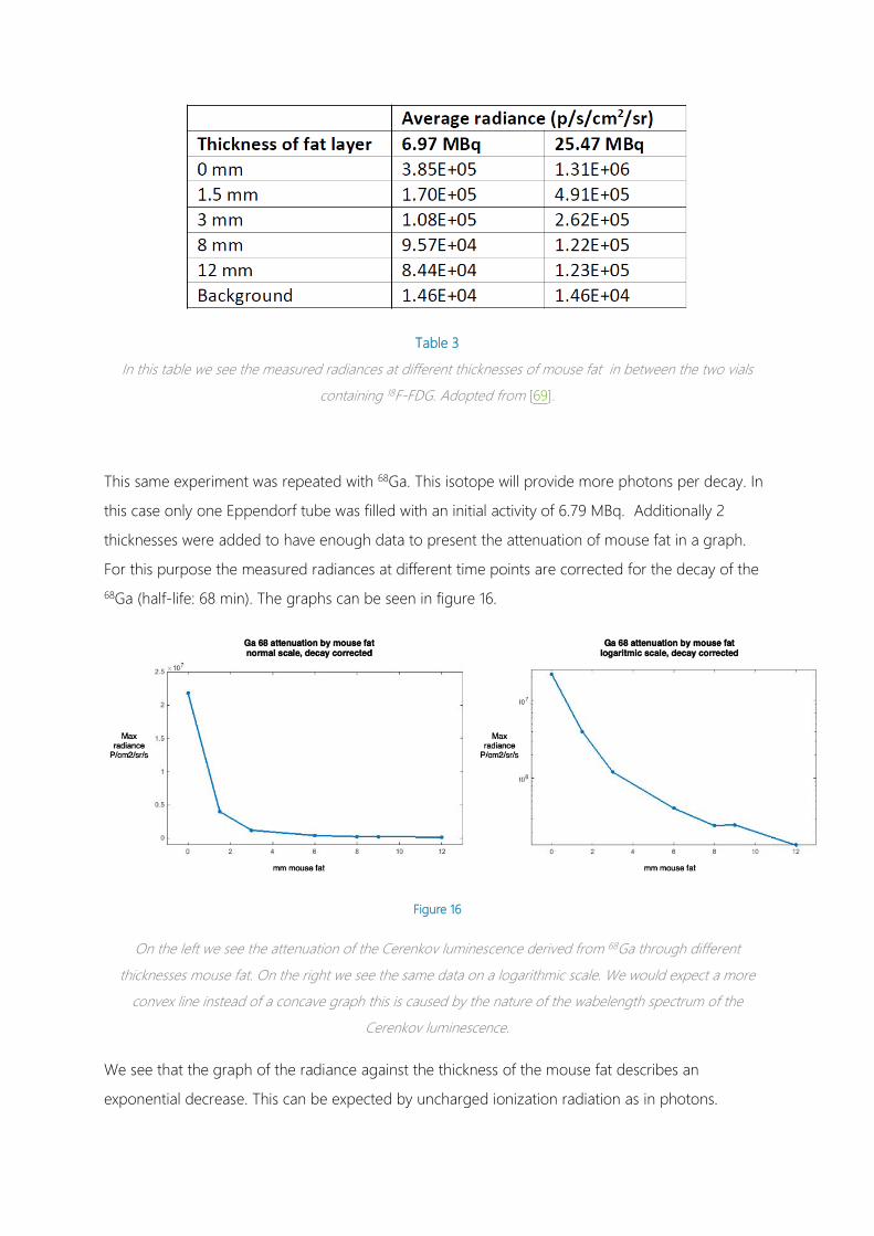
Table 3
In this table we see the measured radiances at different thicknesses of mouse fat in between the two vials
containing 18F-FDG. Adopted from [69].
This same experiment was repeated with 68Ga. This isotope will provide more photons per decay. In
this case only one Eppendorf tube was filled with an initial activity of 6.79 MBq. Additionally 2
thicknesses were added to have enough data to present the attenuation of mouse fat in a graph.
For this purpose the measured radiances at different time points are corrected for the decay of the
68Ga (half-life: 68 min). The graphs can be seen in figure 16.
Figure 16
On the left we see the attenuation of the Cerenkov luminescence derived from 68Ga through different
thicknesses mouse fat. On the right we see the same data on a logarithmic scale. We would expect a more
convex line instead of a concave graph this is caused by the nature of the wabelength spectrum of the
Cerenkov luminescence.
We see that the graph of the radiance against the thickness of the mouse fat describes an
exponential decrease. This can be expected by uncharged ionization radiation as in photons.
43
However, on a semi-logarithmic scale on the right we see that the relation between radiance and
tissue thickness is not exponential and not even shows a convex shape as you expect with a
pointsource. This is influenced by the scatter that occurs in the tissue. Scatter tends to attenuate
even more light with a thicker layer of tissue. However, the inverse exponential nature of the
spectrum of Cerenkov has even more influence on the attenuation curve. Because the majority of
the radiance consists of short wavelengths with low penetrative power the attenuation ratio is the
highest in the beginning. This gives the logarithmic curve a downwards dent. Eventually this leads to
a loss of signal of 95% in the first 3 mm of tissue, 65% in the second 3 mm of tissue and 40 % in the
third 3 mm of tissue. This means that roughly 1 % of the signal will survive 1 cm of prepared mouse
fat.
6.2 ABSOLUTE UPTAKE VALUES OF RADIOPHARMACEUTICALS IN TUMOURS AND
ORGANS
The Cerenkov light derived from radioactive decay is very limited. As stated in the introduction the
amount of light depends mainly on the activity, the energy spectrum of the corresponding isotope
and the refractive index of the medium. Since the amount of light is directly proportional to the
activity it is important to know how much activity is taken up by a tumour. In standard clinical
practice the uptake in a tumour is determined by the SUV (standard uptake value). The SUV is a
simple quantative analysis for the uptake of PET tracers in human tissue. The SUV is calculated as
the ratio between: (1) the radioactivity concentration �𝑐𝑐(𝑡𝑡)� determined by the PET scan and (2) the
administered activity divided by bodyweight. Adjusted for time and decay.
𝑺𝑺𝑺𝑺𝑺𝑺 = 𝒄𝒄(𝒔𝒔)𝑰𝑰𝒏𝒏𝑰𝑰𝑵𝑵𝒄𝒄𝒔𝒔𝑵𝑵𝒅𝒅 𝑺𝑺𝒄𝒄𝒔𝒔𝑾𝑾𝒗𝒗𝑾𝑾𝒔𝒔𝒂𝒂 (𝒔𝒔)
𝑩𝑩𝒔𝒔𝒅𝒅𝒂𝒂𝑩𝑩𝑵𝑵𝑾𝑾𝑺𝑺𝒔𝒔𝒔𝒔� ( 10 )
It presents the uptakes of a certain tissue relative to an imaginary situation were the activity is
equally distributed over the whole body. This means it also provides information on the amount of
activity against the background and thus the tumour to background ratio. This is of course an
important parameter in optical imaging but for the experiments where we want to determine the
sensitity we are interested in what the actual activity in a human tumour is. Therefor we took the
parameter �𝑐𝑐(𝑡𝑡)� from different PET-CT scans of different tumors in different patients.
METHODS
In the database of the nuclear medicine department we have selected patients who underwent an
18F-FDG PET-CT scan who were known to have primary breast tumours, breast metastasis, and
colorectal cancer. For each group we included 10 patients. Evaluation of the images was performed

on the Osirix imaging processing software. To determine the activity we drew a region of interest
(ROI) around the tumour based on the PET and CT data. From this ROI we determined the mean
activity concentration in Bq/mL, the max activity in Bq/mL and the volume of the tumour in mL. We
also did this for patients who received a 68Ga-Dotatate PET-CT scan. Since we determined this is a
potentially valuable isotope for CLI. 68Ga-Dotatate is a fairly different radiopharmaceutical than 18F-
FDG with another distribution pattern and a lower administration dose.
Because the 68Ga scans take place less frequently we studied all types of tumours that were present
in the available patients. We examined the tumours in the same way as we did for the 18F-FDG
scans. Additionally since the distribution of 68Ga accumulates highly in certain organs we determined
the uptake in the thyroid, salivary glands, liver, spleen, kidneys and bladder. We did this to
determine which organs could interfere with Cerenkov imaging.
6.2.1 RESULTS
For the 18F-FDG we selected 10 primary breast tumours, 10 breast metastasis and 10 colorectal
tumours. Additionally we included 2 lung tumours and 4 liver metastasis. We also measured the
uptake in the liver.
The average mean uptake concentration in primary breast tumours was 7.5 kBq/mL (±3.8). For
breast metastasis this was comparable; 7.1 kBq/mL (±4.1). In colorectal cancer the average mean
uptake was slightly higher with concentrations of 12.2 KBq/ml (±3.2). The overall uptake
concentration including the liver metastasis and the lung tumours is 8.9 kBq/ml (±4.0)(Table 4).
For the 68Ga we selected 12 patients. In these 12 patients we found 31 tumours including 11 in the
liver, 8 in lymph nodes throughout the body, 6 in the pancreas, 4 metastasis in the bone and further
in the ileum the breast and in the lung. In addition we have measured the uptake values of the
following organs in all twelve patients; Thyroid liver, spleen, kidneys and the bladder. We could only
find the uptake of the salivary glands in 8 patients.
We saw an average mean uptake concentration of 12.9 kBq/mL (±7.8) in liver tumors.4.7 kBq/mL
(±2.2) for lymph nodes and 16.2 kBq/ml (±15) for pancreas tumours. For all tumours together we
had an average mean uptake of 10.6 kBq/ml (±9.5).
The uptake average uptake in the organs was low for the thyroid and the salivary glands, moderate
for the liver and the kidneys but high for the spleen and exceptionally high 35,4 kBq/mL in the
bladder.

45
Table 4
Absolute uptake values that are determined in PET/CT images. The mean concentration of activity of 10
tumours in 10 different patients are given. In the right two columns the uptake of the most active and least
active tumour are shown. In the 68Ga-Dotatate scans also organs with high physiological uptake have been
included.
On average the tumour uptake of 18F-FDG lies slightly under 10 kBq/mL and for 68Ga slightly over 10
kBq/mL. This gives us an idea of the order of magnitude we should at least be able to detect.
Because we also want to measure in vivo we have attenuation due to the tissue. This means that
produced Cerenkov Luminescence can be detected only partially. Converted back to in vitro studies
this means we should be able to detect even lower concentrations than 10 kBq/mL
What we also can see from this data is that despite the fact 68Ga is administered in lower doses than
18F, pproximately 80 MBq versus around 190 MBq, the absolute dose in the tumour is slightly higher.
As we look at equation 10 we can see that this will result in a SUV that is more than 2 times higher
than that in 18F-FDG. Together with the fact that there is very high uptake in certain organs this
means that there is a relative low uptake in the overall healthy tissue. This means that for tumours
outside the proximity of the high uptake organs there will be a high tumour to background ratio
which is an advantage for optical imaging.

6.2.2 DISCUSSION
From these results it is made clear that we have to be able to detect very small activities. If we want
to perform in vivo imaging we should be able to detect activities of at least lower than 10 kBq/ml. To
determine if this was possible we first consulted the literature. Many articles are published on in vitro
Cerenkov imaging with known activities. In these articles we looked what the lowest activity was they
used or that they could detect. This information can be seen in table 5.
Table 5
Collection of all the studies that have published their results on in vitro CLI. The important factor is what the
lowest activity was they were able to measure. This activity is given in the third and fourth column. The show
the perspective also the isotope the acquisition time and the imaging modality are given. The lowest activity of 18F that is measured is 37 kBq by Liu et al. [1], [14], [26], [29], [33], [34], [39], [42], [44], [66], [70]
In general these studies use high activities for their experiments and especially higher than the
amounts of activity we have found as the uptake in human tumours. There results that came the
closest were the 37 kBq of 18F measured by Liu et al and 39 kBq by Park et al [33], [66]. This is still 4
times higher than the limit we need to be able to detect. Really low activities could be detected for
90Y by Liu and Iodine-124 (124I) and 68Ga by Park. However, according to Gill et al. these emit
respectively 35.8, 6.8 and 25.7 as much photons as 18F [47]. Furthermore it is not really clear if the

47
experiments in these publications tried to find the minimal detectable activity. In many cases they
used convenient measurable amounts like the 37 kBq from Liu et al. which comes down at 1 µCi.
Most of the in vitro experiments are performed in one of the types of IVIS systems by PerkinElmer.
Thorek et al was the first to perform in vivo measurements with an ICCD (Intensified Charge-
Coupled Device) standalone camera. He managed to detect an activity of 100 kBq this is even 10
times as much as we should detect [42]. The last three publications are from a Chinese group who
are developing the ECLI. In this case a fibre scope is attached to the camera which has a smaller
aperture lens. Such a construction leads to a lower intensity than otherwise will be obtained. Due to
the lack of inromation of the numerical aperture not good comparison can be made. Furthermore in
all of the publications they talk about the absolute activity and they do not concern the
concentration of the activity which is an important factor of how intense the luminescence should
be.
Besides the in vivo Cerenkography performed by Thorek et al. We cannot determine from the
literature if it is feasible to image the activity actually taken up by a human tumour. To determine
what the detection limits concerning the activity are we performed our own series of tests.
6.3 MINIMAL DETECTABLE ACTIVITY CONCENTRATION OF 18F-FDG AND 68GA.
Like previous experiments we performed Cerenkov imaging on the IVIS 200 in the animal facility of
the NKI. We performed the imaging on Eppendorf tubes filled with 18F-FDG. We made a dilution
series of 8 Eppendorf tubes to determine the minimal detectable activity concentration.
6.3.1 METHODS
The IVIS system has several options to make acquisitions. The different acquisition settings will result
in changes in the sensitivity of the system, a change in background noise or on total SNR (Signal to
Noise Ratio). These settings were thus of importance for this experiment. There are five parameters
that can be set on the IVIS 200:
• Field of view: There are 5 different settings for the field of view; A,B,C,D and E. They
represent a field of view between 4 cm for A and 25 cm for E. Concurrently with changing
the FOV the object distance gets smaller as the field of view gets smaller. The closer the
object is to the lens, the more light will be detected by the camera and your signal will be
higher.
• F/stop: This represents the aperture of the lens. It controls both the amount of light and the
depth of field of the acquisition. The higher the f-stop number the smaller the aperture and
the less light will be detected by the camera. The choice for a low f/stop number will result

in a high sensitivity but comes at the cost of a small depth of field. The lowest f/stop number
is f/1.
• Binning: With binning you can artificially increase the pixel sizes. This will give a higher
sensitivity because you will catch more signal per pixel but it also comes at the cost of the
spatial resolution. Binning options are 1x1, 2x2, 4x4, 8x8 and 16x16. A binning of 2x2 means
that each pixel is build-up of 4 components. A binning of 4x4 means that each pixel consists
of 16 components. The SNR will have a quadratic improvement with each binning step.
• Exposure time: The amount of time the shutter of the camera is open to make an image.
This number can be chosen from 0.5 seconds. Naturally the longer the exposure time the
more signal will be detected.
• Emission filters: Different types of filters can be placed in front of the CCD camera lens. This
is especially useful for fluorescence and spectral imaging. For bioluminescence and also for
Cerenkov imaging the filter will be left open to obtain the best images.
For our experiment we want to have an acquisition with the most optimal setting to detect a small
activity of 18F. We thus need best possible sensitivity and the highest signal to noise ratio but the
acquisition cannot be too long and the spatial resolution must be sufficient enough to distinct the
shape of the activity. We therefor take the smallest field of view that is possible with the smallest
object distance and we also take the lowest f/stop number to obtain the most signal. We tested
different binning options and exposure times to determine what the best acquisition settings are for
CL detection.
Figure 17
A dilution series is prepared with an initial activity of around 1 MBq in 1ml in the first vial. All the other vials are
filled with 500 µL of water. From the first vial 500 µL is pipetted and mixed with the second vial. We repeat this
for the second vial were we take 500 µL and mix it with the third vial. We do this up to the last vial and after we
mixed this we remove 500 µL. In the end we add 500 µL of water to each vial to obtain the activity that is
shown under the vials per mL
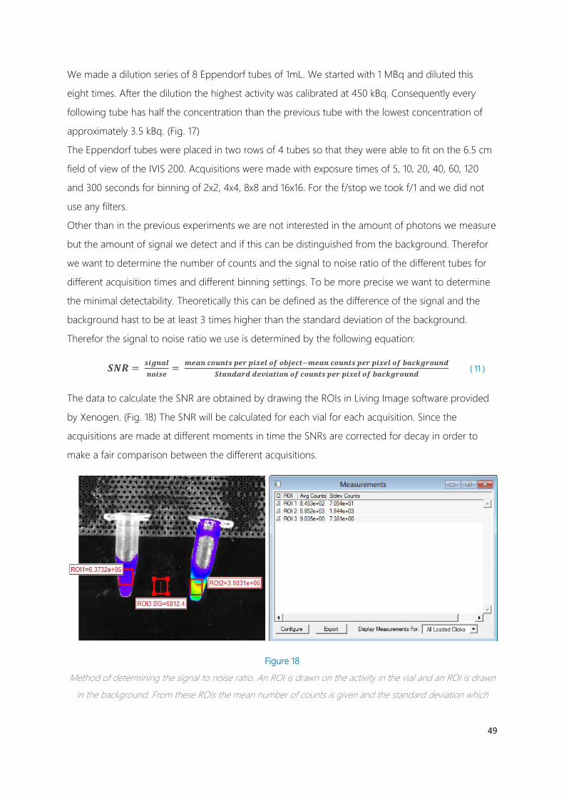
49
We made a dilution series of 8 Eppendorf tubes of 1mL. We started with 1 MBq and diluted this
eight times. After the dilution the highest activity was calibrated at 450 kBq. Consequently every
following tube has half the concentration than the previous tube with the lowest concentration of
approximately 3.5 kBq. (Fig. 17)
The Eppendorf tubes were placed in two rows of 4 tubes so that they were able to fit on the 6.5 cm
field of view of the IVIS 200. Acquisitions were made with exposure times of 5, 10, 20, 40, 60, 120
and 300 seconds for binning of 2x2, 4x4, 8x8 and 16x16. For the f/stop we took f/1 and we did not
use any filters.
Other than in the previous experiments we are not interested in the amount of photons we measure
but the amount of signal we detect and if this can be distinguished from the background. Therefor
we want to determine the number of counts and the signal to noise ratio of the different tubes for
different acquisition times and different binning settings. To be more precise we want to determine
the minimal detectability. Theoretically this can be defined as the difference of the signal and the
background hast to be at least 3 times higher than the standard deviation of the background.
Therefor the signal to noise ratio we use is determined by the following equation:
𝑺𝑺𝑵𝑵𝑺𝑺 = 𝒔𝒔𝑾𝑾𝑺𝑺𝒏𝒏𝑺𝑺𝑺𝑺𝒏𝒏𝒔𝒔𝑾𝑾𝒔𝒔𝑵𝑵
= 𝒎𝒎𝑵𝑵𝑺𝑺𝒏𝒏 𝒄𝒄𝒔𝒔𝒄𝒄𝒏𝒏𝒔𝒔𝒔𝒔 𝒑𝒑𝑵𝑵𝒓𝒓 𝒑𝒑𝑾𝑾𝒅𝒅𝑵𝑵𝑺𝑺 𝒔𝒔𝒐𝒐 𝒔𝒔𝒐𝒐𝑰𝑰𝑵𝑵𝒄𝒄𝒔𝒔−𝒎𝒎𝑵𝑵𝑺𝑺𝒏𝒏 𝒄𝒄𝒔𝒔𝒄𝒄𝒏𝒏𝒔𝒔𝒔𝒔 𝒑𝒑𝑵𝑵𝒓𝒓 𝒑𝒑𝑾𝑾𝒅𝒅𝑵𝑵𝑺𝑺 𝒔𝒔𝒐𝒐 𝒐𝒐𝑺𝑺𝒄𝒄𝒌𝒌𝑺𝑺𝒓𝒓𝒔𝒔𝒄𝒄𝒏𝒏𝒅𝒅𝑺𝑺𝒔𝒔𝑺𝑺𝒏𝒏𝒅𝒅𝑺𝑺𝒓𝒓𝒅𝒅 𝒅𝒅𝑵𝑵𝒗𝒗𝑾𝑾𝑺𝑺𝒔𝒔𝑾𝑾𝒔𝒔𝒏𝒏 𝒔𝒔𝒐𝒐 𝒄𝒄𝒔𝒔𝒄𝒄𝒏𝒏𝒔𝒔𝒔𝒔 𝒑𝒑𝑵𝑵𝒓𝒓 𝒑𝒑𝑾𝑾𝒅𝒅𝑵𝑵𝑺𝑺 𝒔𝒔𝒐𝒐 𝒐𝒐𝑺𝑺𝒄𝒄𝒌𝒌𝑺𝑺𝒓𝒓𝒔𝒔𝒄𝒄𝒏𝒏𝒅𝒅
( 11 )
The data to calculate the SNR are obtained by drawing the ROIs in Living Image software provided
by Xenogen. (Fig. 18) The SNR will be calculated for each vial for each acquisition. Since the
acquisitions are made at different moments in time the SNRs are corrected for decay in order to
make a fair comparison between the different acquisitions.
Figure 18
Method of determining the signal to noise ratio. An ROI is drawn on the activity in the vial and an ROI is drawn
in the background. From these ROIs the mean number of counts is given and the standard deviation which

determines how noisy the signal is. The mean of the background is subtracted from the average signal from the
activity. This is then divided by the standard deviation of the background.
6.3.2 RESULTS
From the results we could confirm that as expected the relation between the activity and the SNR is
linear as well as the relation between exposure time and the SNR. We could also confirm the
quadratic relation between the binning and the SNR. This means that we obtained the highest signal
to noise ratio for the higher activities, the longer exposure times and the highest binning. We
obtained a SNR of 737 for the 450 kBq/ml vial an exposure time of 300 seconds and 16x16 binning.
(Fig. 19) More interesting was the activity that was the least detectable to determine the limits of the
imaging device. Theoretically the SNR has to exceed 3 for the signal to be detectable. In 4 of the 28
acquisitions the SNR for the least active vial exceeded this threshold. In the 300 second acquisition
with 8x8 binning and for the 60, 120 and 300 second acquisition with 16x16 binning. This means that
we are practically able to detect activity concentrations of 3.5 kBq per mL but at the cost of long
exposure times and extensive binning.
Figure 19
Image of the dilution series containing 18F performed on the IVIS 200. This is a 300 second acquisition with the
highest amount of binning 16x16. We can distinct all the vials from the background including the one with the
least activity. The signal to noise ratio for this particular vial was 13.85.

51
6.4 DETERMINING THE BEST STANDALONE CAMERA AND ITS MINIMAL
DETECTABILITY
Since we want to determine the clinical feasibility of CLI we cannot use a system as the IVIS 200 but
we have to make use of another type of commercially available camera. This camera has to be a
standalone camera and preferably an EMCCD camera. As mentioned in chapter 5 EMCCD cameras
will give the best performance for low light imaging as is the case in CLI. We made a selection of
commercially available EMCCD cameras and a few other types of cameras that have been used in
CLI and made a comparison based on their specifications. Because we wanted to know what the
minimal detectable activity was we needed the most sensitive camera which provides the best SNR.
Important are thus the factors that determine the sensitivity and the noise of the camera.
The most important specifications are on the one hand the QE which determines the sensitivity of
the CCD chip and on the other hand the mechanisms that contribute to the total noise floor. These
mechanisms are the amount of chip cooling that will have an effect on the dark current, the readout
noise and the clock induced charge. Furthermore the gain possibilities and the resolution of the chip
are of importance.
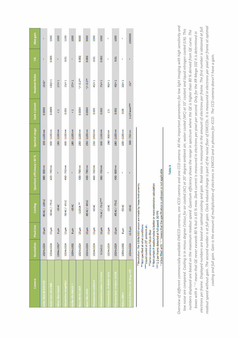
Tabl
e 6
Ove
rvie
w o
f diff
eren
t com
mer
cial
ly a
vaila
ble
EMCC
D ca
mer
as, o
ne IC
CD c
amer
a an
d on
e CC
D ca
mer
a. A
ll th
e im
port
ant p
aram
eter
s for
low
ligh
t im
agin
g w
ith h
igh
sens
itivi
ty a
nd
low
noi
se a
re c
ompa
red.
Coo
ling
is in
min
us d
egre
e Ce
lsius
for a
ir co
oled
(AC)
at 2
0˚ d
egre
e am
bien
t air,
wat
er c
oole
d (W
C) a
t 10˚
coo
lant
and
liqu
id n
itrog
en c
oole
d (L
N).
This
num
bers
disp
laye
d ar
e ba
sed
on th
e m
axim
um re
adou
t spe
ed. Q
uant
um e
ffici
ency
show
s the
rang
e in
spec
trum
whe
re th
e Q
E is
high
er th
an 8
0 %
der
ived
from
QE
curv
e. T
he
boxe
s with
a '
~' m
ean
that
QE
neve
r exc
eeds
80
% b
ut is
65
% m
ax. D
ark
curr
ent i
s mea
sure
d in
ele
ctro
ns p
er p
ixel
per
seco
nd. O
nly
for t
he X
R M
ega
10Z
it is
dete
rmin
ed in
el
ectr
ons p
er fr
ame.
Disp
laye
d nu
mbe
rs a
re b
ased
on
optim
al c
oolin
g an
d ga
in. R
ead
noise
is m
easu
red
in th
e am
ount
of e
lect
rons
per
fram
e. T
he fi
rst n
umbe
r is o
btai
ned
at fu
ll re
adou
t spe
ed w
ithou
t gai
n. T
he se
cond
num
ber i
s at f
ull g
ain.
Clo
ck in
duce
d ch
arge
is p
art o
f the
noi
se fl
oor o
f EM
CCDs
. It i
s mea
sure
d in
ele
ctro
ns p
er p
ixel
per
fram
e at
opt
imal
co
olin
g an
d fu
ll ga
in. G
ain
is th
e am
ount
of m
ultip
licat
ion
of e
lect
rons
in E
MCC
D an
d in
pho
tons
for I
CCD.
The
CCD
cam
era
does
n’t h
ave
a ga
in.

53
As we can see from table 6 there are two types of chips manufactured. The chips made by Texas
instruments show inferior specifications than the other chips. They are not cooled to extreme low
temperatures and besides they lack the information on the QE. The rest of the chips show to have a
similar quantum efficiency. The big difference is made in the cooling possibilities and the
performances on the different types of noise. We have selected 4 cameras that in our opinion
promised the best performance for low light imaging (Fig. 20):
• Andor iXon ultra 888
• Princeton ProEM+ 1024b
• Nüvü Hnü 1024
• Hamamatsu ImagEMx2
We have tested these four cameras in our own build setup in a similar way as we did in the previous
experiment on the IVIS. In this way we tried to determine what camera is the best and at the same
time determine the limit for Cerenkov luminescence detection.

Figure 20
The 4 different EMCCD cameras that were tested.
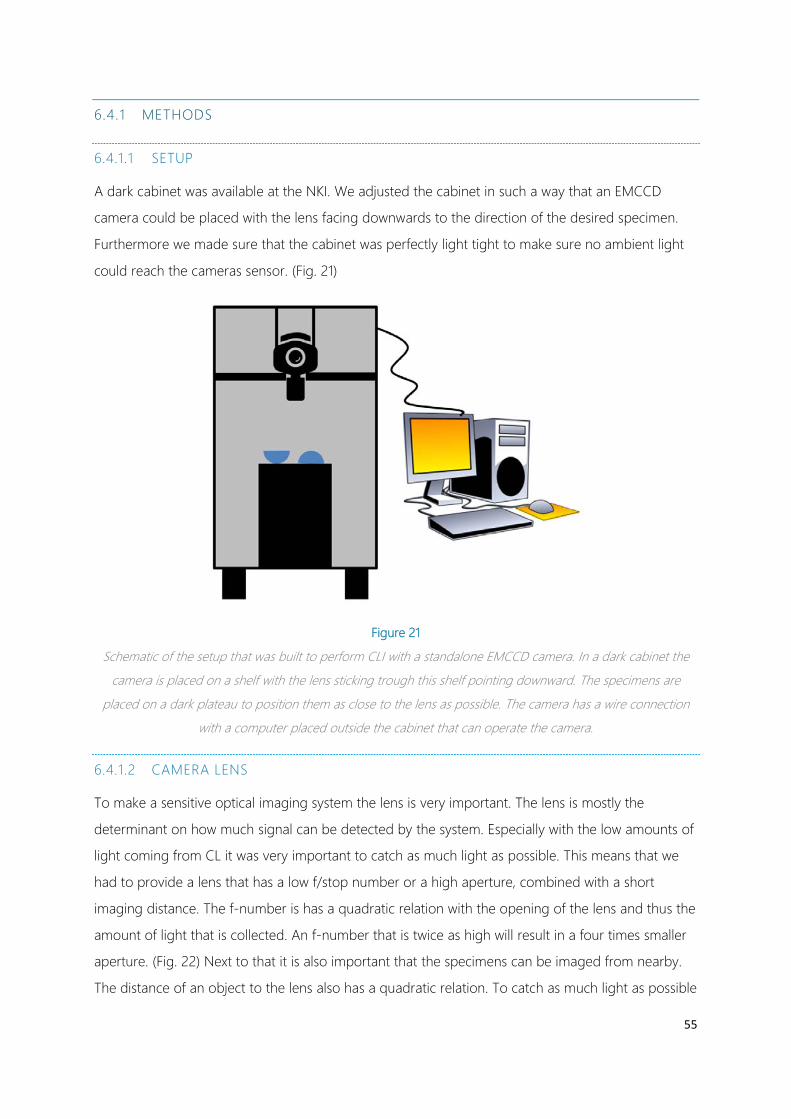
55
6.4.1 METHODS
6.4.1.1 SETUP
A dark cabinet was available at the NKI. We adjusted the cabinet in such a way that an EMCCD
camera could be placed with the lens facing downwards to the direction of the desired specimen.
Furthermore we made sure that the cabinet was perfectly light tight to make sure no ambient light
could reach the cameras sensor. (Fig. 21)
Figure 21
Schematic of the setup that was built to perform CLI with a standalone EMCCD camera. In a dark cabinet the
camera is placed on a shelf with the lens sticking trough this shelf pointing downward. The specimens are
placed on a dark plateau to position them as close to the lens as possible. The camera has a wire connection
with a computer placed outside the cabinet that can operate the camera.
6.4.1.2 CAMERA LENS
To make a sensitive optical imaging system the lens is very important. The lens is mostly the
determinant on how much signal can be detected by the system. Especially with the low amounts of
light coming from CL it was very important to catch as much light as possible. This means that we
had to provide a lens that has a low f/stop number or a high aperture, combined with a short
imaging distance. The f-number is has a quadratic relation with the opening of the lens and thus the
amount of light that is collected. An f-number that is twice as high will result in a four times smaller
aperture. (Fig. 22) Next to that it is also important that the specimens can be imaged from nearby.
The distance of an object to the lens also has a quadratic relation. To catch as much light as possible

you want the object to be as close to the lens as possible. Therefor a short focus distance is required
to obtain a short object distance without compromising the sharpness of the image.
Figure 22
A representation of the different f/stop numbers that indicate the aperture. We see that a quadratic relation
between the f/stop number and the area of the aperture. This means that a twice as low f/stop number leads
to a four time increase in signal. Adopted from www.gotosnapshot.com
Figure 23
Here we see a schematic of the CCD sensor and different image projection surfaces of different lens formats.
The sensor in red, is 13 by 13 mm. You would think this would have the best fit with a ½”. However, lens
formats are measured by the diagonal of the square the circle just fits in. This means that for this CCD chip we
need a 1” lens format to make use of the entire CCD chip.
For our experiments we selected the best option that was available in house and was compatible
with all the EMCCD cameras (C-mount). We had the opportunity to use a Pentax TV lens with a
focal distance of 8.5 mm and a maximal aperture of f/1.5. This led to a minimal object distance of

57
20 cm. However, the format of the lens, a manufacturing parameter of the housing combined with
the mount, was a 2/3”. This meant that the CCD chip which have a size of 13x13 mm are not fully
utilized. (Fig. 23) Preferably we would like a 1” format lens.
6.4.1.3 ACQUISITION
The cameras were delivered with the corresponding software to operate the camera. Besides the
options that were available in the IVIS system the different EMCCD systems provided a lot more
options to set up different acquisitions. There are different readout modes, you can choose not only
times for the exposure but also the rate of readout. Furthermore you can choose the speed of the
storage shift on the chip and the pixel rate of the analogue to digital converter. Additionally the
temperature of the chip can be set and there are different options to perform corrections. These
settings will have a huge effect on the resulting image. Especially the noise levels can be tweaked for
any other acquisition setting.
It was not a simple task to find out what the optimal acquisition options are because many of the
settings are interdependent. For instance the speed of the readout should be matched with the gain
and the exposure time. Also for all cameras the setting options were slightly different and the
behaviour of each camera was unique. Some cameras were more prone to noise than others and
other cameras showed artefacts if the settings were not fully optimized.
The performance of the camera and the ease of use was very important. Next to that we wanted to
know which camera could provide us with the highest SNR when imaging a certain amount of
radioactivity. Therefor we did not compare the cameras in the exact same settings but we tested
them all to their limits to compare their overall performance. This means that all the parameters that
were not camera dependent were kept the same: the used lens, the distance between the lens and
the specimens, the exposure time and the amount of binning. Although the activity in the vials of
the dilution series was not always the same we can easily correct for this since it shows a linear
relation.
With each camera we have performed a series of acquisitions on the dilution series with 18F and
68Ga. We chose the acquisition settings that after extensive testing showed the best performance. As
with the experiments on the IVIS we compared different acquisition times but additionally we also
made acquisitions with different EM gains. To compare the different acquisitions for a camera with
each other we compared the SNR of the highest active vial. Next to that we determined the lowest
detectable activity for the best 60 second acquisition and the best 300 second acquisition.

6.4.2 RESULTS
6.4.2.1 ANDOR IXON ULTRA 888
With the Andor camera we were able to obtain nice images without any gain. This is the so called
conventional mode. For longer acquisitions however, a lot of ‘cosmic rays’, saturated pixels due
to gamma rays falling directly on the camera chip, appeared. The software had no options to
remove this data from the image. In the conventional modes these dots could be ignored. However,
when the EM-gain was increased to a certain amount the cosmic rays resulted in a horizontal
striking pattern. This is an artefact caused by charge transfer efficiency problems. A phenomenon
known to EMCCD’s when pixels in the gain register pack to many electrons [67]. As a result
acquisitions with long exposure times and high EM-gain are useless. (Fig. 24)
Figure 24
Raw data images of the dilution series made with the Andor EMCCD camera. We can see a lot of incident
gamma rays which will disturb the images significantly. Especially when the EM-gain is applied, upper right, this
will lead to horizontal patterns that distort a lot of the data. On the lower left we see an image made with 68Ga.
Due to higher light production lower activities can be used which lead to less gamma rays and consequently a
better distinction with the background. Also there is less binning required (1x1 instead of 4x4) which results in a
higher resolution.

59
6.4.2.2 PRINCETON INSTRUMENTS PROEM + 1024B
The performance of the ProEm for the 18F dilution series was a little bit poor, and definitely less than
the Andor. An explanation for this performance can be that there was some degree of light leakage
into the light tight cabinet. This can be seen by the brighter circle in the centre which represents the
aperture of the lens. For the 68Ga dilution series no such thing could be detected. These resulted in
very clear images of the activity up to low levels of activity. The striking artefacts caused by CTE
problems was not present in this camera.(Fig 25)
Figure 25
Selection of the results made with the Princeton instruments EMCCD camera. Above we see the 18F dilution
series. Only a few of higher active vials can be detected. Only several hundreds of kBq/ml can be distinguished.
We can also see a bright circle in the middle of the images. This is the projection surface of the 2/3” lens. This
means that there was some ambient light present during the acquisitions. The images with the 68Ga again show
more clear images and the vial of 21 kBq/ml can be distinguished.
6.4.2.3 NÜVÜ HNÜ 1024
The Nüvü camera was the one which had the best specifications and therefor the expectations of
the performance were high. Unfortunately the company that manufactured the camera is a new kid
on the block and this was reflected by the provided software that gave a lot of problems. As a
consequence we were not able to perform exposure times longer than 30 seconds and even these
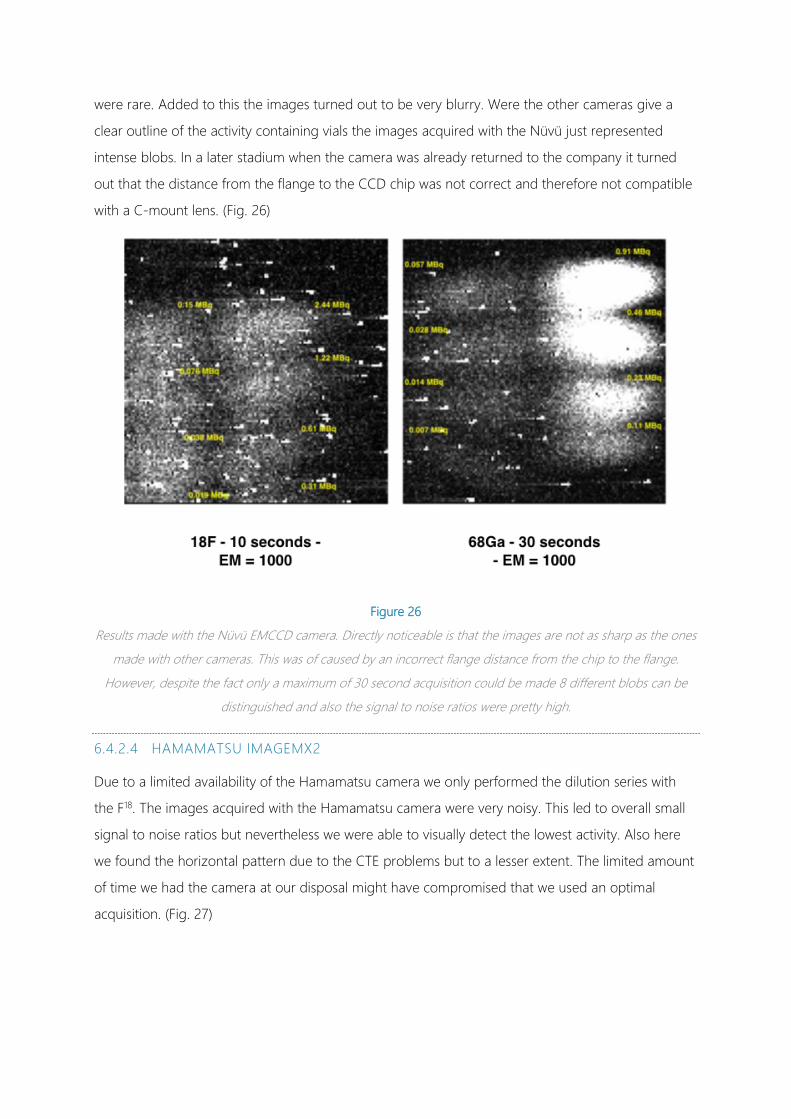
were rare. Added to this the images turned out to be very blurry. Were the other cameras give a
clear outline of the activity containing vials the images acquired with the Nüvü just represented
intense blobs. In a later stadium when the camera was already returned to the company it turned
out that the distance from the flange to the CCD chip was not correct and therefore not compatible
with a C-mount lens. (Fig. 26)
Figure 26
Results made with the Nüvü EMCCD camera. Directly noticeable is that the images are not as sharp as the ones
made with other cameras. This was of caused by an incorrect flange distance from the chip to the flange.
However, despite the fact only a maximum of 30 second acquisition could be made 8 different blobs can be
distinguished and also the signal to noise ratios were pretty high.
6.4.2.4 HAMAMATSU IMAGEMX2
Due to a limited availability of the Hamamatsu camera we only performed the dilution series with
the F18. The images acquired with the Hamamatsu camera were very noisy. This led to overall small
signal to noise ratios but nevertheless we were able to visually detect the lowest activity. Also here
we found the horizontal pattern due to the CTE problems but to a lesser extent. The limited amount
of time we had the camera at our disposal might have compromised that we used an optimal
acquisition. (Fig. 27)
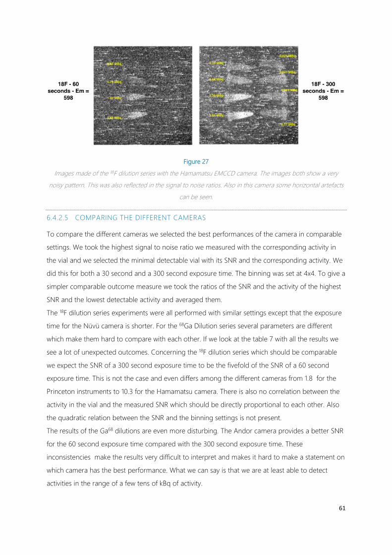
61
Figure 27
Images made of the 18F dilution series with the Hamamatsu EMCCD camera. The images both show a very
noisy pattern. This was also reflected in the signal to noise ratios. Also in this camera some horizontal artefacts
can be seen.
6.4.2.5 COMPARING THE DIFFERENT CAMERAS
To compare the different cameras we selected the best performances of the camera in comparable
settings. We took the highest signal to noise ratio we measured with the corresponding activity in
the vial and we selected the minimal detectable vial with its SNR and the corresponding activity. We
did this for both a 30 second and a 300 second exposure time. The binning was set at 4x4. To give a
simpler comparable outcome measure we took the ratios of the SNR and the activity of the highest
SNR and the lowest detectable activity and averaged them.
The 18F dilution series experiments were all performed with similar settings except that the exposure
time for the Nüvü camera is shorter. For the 68Ga Dilution series several parameters are different
which make them hard to compare with each other. If we look at the table 7 with all the results we
see a lot of unexpected outcomes. Concerning the 18F dilution series which should be comparable
we expect the SNR of a 300 second exposure time to be the fivefold of the SNR of a 60 second
exposure time. This is not the case and even differs among the different cameras from 1.8 for the
Princeton instruments to 10.3 for the Hamamatsu camera. There is also no correlation between the
activity in the vial and the measured SNR which should be directly proportional to each other. Also
the quadratic relation between the SNR and the binning settings is not present.
The results of the Ga68 dilutions are even more disturbing. The Andor camera provides a better SNR
for the 60 second exposure time compared with the 300 second exposure time. These
inconsistencies make the results very difficult to interpret and makes it hard to make a statement on
which camera has the best performance. What we can say is that we are at least able to detect
activities in the range of a few tens of kBq of activity.
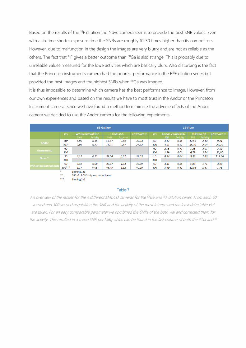
Based on the results of the 18F dilution the Nüvü camera seems to provide the best SNR values. Even
with a six time shorter exposure time the SNRs are roughly 10-30 times higher than its competitors.
However, due to malfunction in the design the images are very blurry and are not as reliable as the
others. The fact that 18F gives a better outcome than 68Ga is also strange. This is probably due to
unreliable values measured for the lowe activities which are basically blurs. Also disturbing is the fact
that the Princeton instruments camera had the poorest performance in the F18F dilution series but
provided the best images and the highest SNRs when 68Ga was imaged.
It is thus impossible to determine which camera has the best performance to image. However, from
our own experiences and based on the results we have to most trust in the Andor or the Princeton
Instrument camera. Since we have found a method to minimize the adverse effects of the Andor
camera we decided to use the Andor camera for the following experiments.
Table 7
An overview of the results for the 4 different EMCCD cameras for the 68Ga and 18F dilution series. From each 60
second and 300 second acquisition the SNR and the activity of the most intense and the least detectable vial
are taken. For an easy comparable parameter we combined the SNRs of the both vial and corrected them for
the activity. This resulted in a mean SNR per MBq which can be found in the last column of both the 68Ga and 18

63
7 CLINICAL PILOT STUDIES
7.1 HUMAN IN VIVO CLI STUDY
7.1.1 RATIONALE FOR THE STUDY
In the first experiments we have proven in vitro that we are able to detect activities, in accordance
with the actual uptake in human tumours. This is of course a favourable setting with transparent
substances and vials. Translation of this technique from a preclinical setting into the operating room
has led to a is another challenge. One of the biggest issues is the spectral character of the Cerenkov
light. Blue light is generally well attenuated by perfused tissue, thus the penetration depth of this
light is in the order of a few millimetres. For a superficial tumour in the skin, like the mouse tumour
models often used in a preclinical setting, this is not a problem and enough light will reach the CCD
camera. Obviously, humans are much bigger than mice and tumours are not always located in the
skin. Imaging of Cerenkov light in-vivo will be a much tougher assignment. This means that, before
we start using a CCD camera in a surgical setting, we have to prove that we are able to make
clinically relevant images with the available techniques. With clinical relevant images we mean
exactly comparable to actual uptake activity in real human tissue. To do this we want to image
actual tumour in living human beings.
This is not an easy task since cancer patients with administered activity are required and
subsequently the tumour has to be accessible with the EMCCD camera. To prevent invasive
methods and additional doses of radiopharmaceuticals we selected a special group of patients for
this pilot study. Patients with relatively superficial tumours that are already scheduled for diagnostic
or follow-up 18F-FDG or 68Ga-Dotatate PET imaging are asked to participate in this study.
7.1.2 METHODS:
PATIENT SELECTION:
Eligible patients are patients of the NKI-AvL which will undergo a routine 18F-FDG PET-CT scan. The
inclusion criteria are:
• Scheduled for a routine 18F-FDG PET-CT scan.
• Patients with a superficial tumour. (< 2 cm from surface)
• Any tumour type can be included however, it must show sufficient uptake during the PET-
CT scan.
• Written informed consent should be provided.

• Patients ≥ 18 years old
The exclusion criteria are:
• Melanomas with high melanin levels as determined by visual assessment prior to the PET/CT
scan because melanin can absorb a lot of light.
Patients will be selected after they are planned for a PET-CT scan. This planning occurs for the
majority of the patients one or two weeks prior to the PET-CT scan. If patients are scheduled the
researcher will screen their dossier to determine if they have a superficial tumour. This will be done
based on the PET-CT indication, clinical dossier and when available prior CT, PET-CT or MRI scans.
When patients are eligible they will be contacted by telephone to confirm if they really have a
tumour at the moment and are up for a PET-scan. They are informed on the study and asked to
join, additionally patient information will be sent by post or e-mail. The decision to join the study
and informed consent will be asked at the day of the investigation, prior to the PET-CT scan. When
a patient decides to participate, informed consent will be signed.
Taking into account possible errors and the fact that we want to measure tumours at different
depths in the patient we have set the maximum sample size at 12 patients in total. After each patient
an evaluation is made on the feasibility of the camera set-up. If it is necessary the imaging protocol
will be modified. When sufficient data is acquired to answer the question within the 12 patients the
study will not be continued.
7.1.2.1 ROOM PREPARATION HOW TO MAKE IT DARK
For the imaging of the patients a special room was available near the nuclear department. This
room had only a small window to the hallway and was therefore relatively perfect to eliminate as
much light as possible. To make to room as dark as possible the window was covered with
aluminium foil on the outside and a darkening cloth on the inside. The slits around the door were
covered by an extra layer of insulation strips on the inside of the door frame. Additionally, the slits
were covered on the inside by more darkening cloth. In the room all tiny light sources such as LEDs
from different devices were covered with black aluminium tape. The fluorescent tube lights were off
for at least an hour in advance of the experiments to minimize the afterglow.
The light elimination was checked by making images with the EMCCD camera with a high gain from
every corner of the room. The most prominent light source left was the keyhole in the door which
was also covered with black aluminium tape. However, there was still some degree of light in the
room but it was not clear where exactly this came from. It might have been photons in the NIR
region coming through the suspended ceiling.
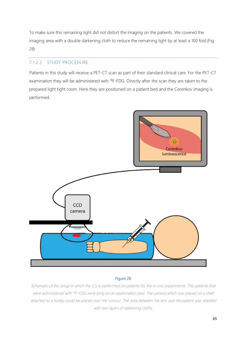
65
To make sure this remaining light did not distort the imaging on the patients. We covered the
imaging area with a double darkening cloth to reduce the remaining light by at least a 100 fold.(Fig.
28)
7.1.2.2 STUDY PROCEDURE
Patients in this study will receive a PET-CT scan as part of their standard clinical care. For the PET-CT
examination they will be administered with 18F-FDG. Directly after the scan they are taken to the
prepared light tight room. Here they are positioned on a patient bed and the Cerenkov imaging is
performed.
Figure 28
Schematic of the setup in which the CLI is performed on patients for the in vivo experiments. The patients that
were administered with 18F-FDG were lying on an examination bed. The camera which was placed on a shelf
attached to a trolley could be placed over the tumour. The area between the lens and the patient was shielded
with two layers of darkening cloths.
All patients will undergo the following procedures:
• Standard clinical care:
o Patients are administered with 18F-FDG.
o Patients will receive a PET-CT scan as usual.
• Procedures related to this study:
o After the PET-CT scan is finished patients are taken to a prepared light tight room at
the nuclear medicine department.
o In the CLI room patients will be placed on an examination bed with the site of the
tumour uncovered and accessible for the camera.
o The camera will be positioned in the direction of the tumour.
o Darkening cloths are positioned around the camera and the tumour location.
o Multiple acquisitions will be performed in total darkness while the patient remain
still. Acquisition times vary from 1 to 300 seconds.
o When the imaging is finished, the patient is ready to go home.
The CLI examination will take place roughly two hours after the administration of the
radiopharmaceutical. The total CLI procedure will take no more than 30 minutes.
STUDY PARAMETERS
Based on the PET-CT scan the absolute uptake of the concerned tumour will be determined in the
same way as is done in chapter 6.2. Additionally the distance from the surface of the tumour to the
surface of the skin will be determined. This will be used to correlate the acquired signal to the depth
and the activity.
The images will be analysed and the number of counts per pixel will be determined for two regions
of interest (ROI) for each tumour (Fig 28).

67
Figure 29
Timeline of the study procedure as it will be carried out for patients that will have an 18F-FDG PET scan. This
includes a fasting period of 6 hours prior to administration and an exposure period of an hour before the PET-
CT scan.
The first ROI will represent the healthy tissue around the tumour and thus can be seen as
background. The second ROI will be located on top of the tumour and will represent the tumour
signal. The number of counts derived from the tumour should be related to the radioactivity in the
tumour and the depth of the tumour within the tissue. From the mean number of counts in each
ROI and the standard deviations (SD) the signal to noise ratio and thus the detectability can be
determined. The signal will be the mean number of counts in ROI 2 and the noise will be the SD in
the number of counts in ROI 1. The signal to noise ratio will be the following:
𝑺𝑺𝑵𝑵𝑺𝑺 = 𝒔𝒔𝑾𝑾𝑺𝑺𝒏𝒏𝑺𝑺𝑺𝑺𝒏𝒏𝒔𝒔𝑾𝑾𝒔𝒔𝑵𝑵
= 𝑴𝑴𝑵𝑵𝑺𝑺𝒏𝒏 𝑺𝑺𝑹𝑹𝑰𝑰 𝟐𝟐−𝑴𝑴𝑵𝑵𝑺𝑺𝒏𝒏 𝑺𝑺𝑹𝑹𝑰𝑰 𝟏𝟏𝑺𝑺𝑺𝑺 𝑺𝑺𝑹𝑹𝑰𝑰 𝟏𝟏
( 12 )
If the SNR is larger than 3, the tumour can theoretically be distinguished from the background.

Figure 30
If the dashed red circle represents the tumour the blue square will be the imaging area that is captured with the
camera. From these images the counts per pixel will be determined for 2 ROIs: ROI 1 will be measured a few cm
outside the tumour area and consist of healthy tissue . ROI 2 will be measured at the site of the tumour.
The ultimate goal eventually is to visualize a tumour based on its Cerenkov luminescence. Therefor
we will perform image processing to select the signal from the background noise and other
disturbing factors such as incident gamma rays. Thereafter this processed image is overlaid with a
light image that shows the view of the imaged area. This will lead to an intensity map of the
Cerenkov signal over the normal photo just like is done for the images of the IVIS. This will be done
independently by two researchers by different methods:
Matlab
The raw data that was made with the camera software is loaded into Matlab. First the cosmic rays
are removed by selecting a threshold that will eliminate all pixels above that value. These pixels are
replaced with the average of their surroundings. After that the image is smoothed. The noise floor is
removed by providing another threshold that eliminates all pixels below a certain value. What is left
is the signal caused by CLI. Of this signal an intensity colormap is produced which is overlaid with
the light image.

69
ImageJ
The raw data is opened in ImageJ. The image is processed by using successively the ‘Remove
Outliers’, algorithm and the despeckle function to get rid of the cosmic rays. Subsequently the
image is smoothed. The image is then merged with the light image in MIPAV (Medical Image
Processing, Analysis, and Visualization). This program enables to set an intensity scaled colormap for
one of the datasets.
Table 8
Characteristics of the 5 included patients for the in vivo CLI study. The distance of the tumour to the surface,
the SUVmax and the mean activity are based on the PET-CT scan that was made prior to the CLI. The SNR was
determined on the CLI images.
7.1.3 RESULTS:
For this study we have included a total of 5 patients. The main reason only 5 patients were included
is that the trial period of the camera ended before we could include more patients. The relevant
characteristics of the patients can be seen in table 8. Among these 5 patients were patients with
ideal conditions to perform CLI on. Ideal conditions are tumours that are very superficial with a high
uptake value. Especially the third subject seemed very promising with a tumour directly at the
surface of the lower leg and with high uptake values with an average of 7.7 kBq/ml and a SUVmax
of 11.7. On all of the patients acquisitions up to 300 seconds were performed. In patient number
two were the tumour was located on the hand there was light leakage through the darkening cloth
which resulted in a useless result. From then on we used two separate darkening cloths to prevent
any light from contaminating the imaging.
In none of the images with acquisition shorter than 300 seconds any signal could be detected. For
the 300 second acquisition in the first patient we did detect a signal. As you can see from the SNR
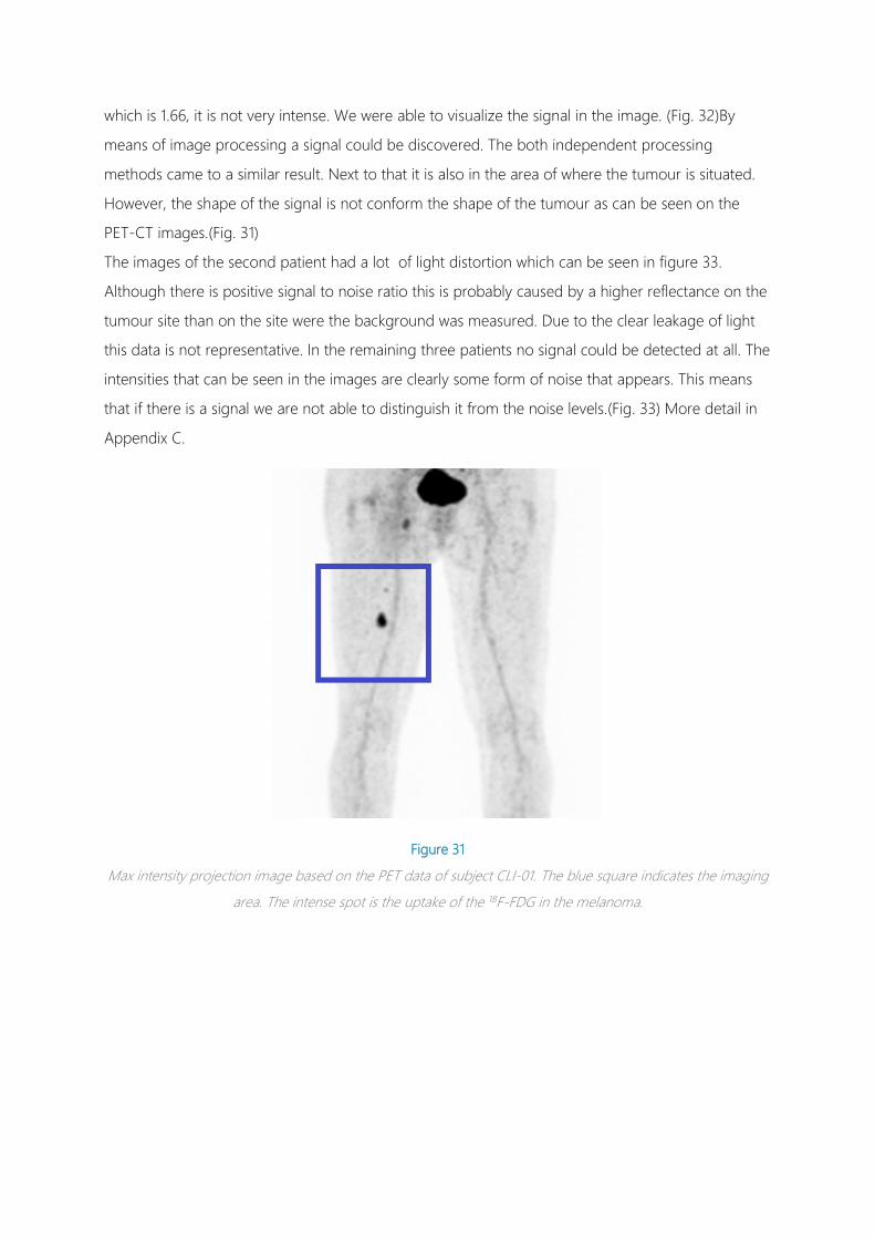
which is 1.66, it is not very intense. We were able to visualize the signal in the image. (Fig. 32)By
means of image processing a signal could be discovered. The both independent processing
methods came to a similar result. Next to that it is also in the area of where the tumour is situated.
However, the shape of the signal is not conform the shape of the tumour as can be seen on the
PET-CT images.(Fig. 31)
The images of the second patient had a lot of light distortion which can be seen in figure 33.
Although there is positive signal to noise ratio this is probably caused by a higher reflectance on the
tumour site than on the site were the background was measured. Due to the clear leakage of light
this data is not representative. In the remaining three patients no signal could be detected at all. The
intensities that can be seen in the images are clearly some form of noise that appears. This means
that if there is a signal we are not able to distinguish it from the noise levels.(Fig. 33) More detail in
Appendix C.
Figure 31
Max intensity projection image based on the PET data of subject CLI-01. The blue square indicates the imaging
area. The intense spot is the uptake of the 18F-FDG in the melanoma.

71
Figure 32
On the left we see the light images made of the imaging area that is seen in figure 31. The red circle indicates
where the tumour is located. In the middle we see a merged image of the light image and the CLI image
processed with Matlab. On the right we see the merged image of the light image and the CLI image processed
in ImageJ.
Figure 33
Merged images the light image and the processed CLI image. The CLI images have an exposure time of 300
seconds and a binning of 8x8, CLI 1-3, or 4x4, CLI 4 and 5. The red circles indicate the location of the tumour.
In none of the images there is a correct correlation between the obtained signal and the location of the
tumour.

7.1.4 DISCUSSION
The results show that only in the first patient there was some signal detected that could be derived
from Cerenkov luminesnce. However, it is highly likely that the signal is derived from some other
source. First of all the shape of the signal does not exactly match the shape and position of the
tumour. Next to that we found much higher activities of 18F in more superficial tumours in patient 3
and 5 in which we were not able to detect any signal here. This means that if we have detected
Cerenkov radiation in the first patients we should have definitely detected it in patient 3 and 5.
Moreover during the first two patients only one darkening cloth was used to cover the imaging area.
In the second case it is very clear that there is light leakage since the intensity of the dark image
corresponds to the brighter areas of the light image. This makes it more likely that the intensity is
caused by reflectance of some light leakage.
The conclusion is thus that we are not able to detect any activity. In the first two cases a possible
explanation could be the light leakage. It is evident that any slight amount of light will overshadow
the Cerenkov luminescence signal. In the last three cases light leakage could not be detected in the
images. However, the histogram data tells us that in any case there was at least some ambient light
in the data. (Fig. 34)
Figure 34
A method to check if there is ambient light distorting the acquisition is by looking at the histogram of the
counts. We see two histograms with the same range from 500-700. On the left we see an acquisition that is
made with the lens cap on so there is no ambient light at all. We see a very high peak around the offset of 500.
On the right a histogram is shown of an acquisition that was contaminated with light leakage. We can see that
each pixel starts with an offset of at least 600 counts.

73
Furthermore it can be explained why we can’t detect any activity by the results of our previous
experiments. In an in vitro experiment in ideal settings with near perfect darkness and transparent
phantoms we were only able to barely detect an activity concentration of around 20 kBq/ml. The
activities in these patients at the moment of the PET-CT scan are more than twice as low. Due to the
decay the activities would be even lower at the moment of the CLI experiments. Next to that the
activity was situated in human tissue covered by the epidermis which causes a lot of absorbance and
scattering of the Cerenkov light. Based on the experiments in mouse fat this will lead to a loss of
95% in the first 3 mm of tissue. This means that we are dealing with an intensity that is
approximately 50 times lower than the lowest intensity we were able to detect so far.
7.1.4.1 COSMIC RAYS
The cosmic rays showed to have a lot of influence on the CLI imaging. Especially when longer
exposure times or the gain was used. These cosmic rays are caused by the gamma rays that are
coming from the patient which is at that moment very active. In experiments with the second subject
were the tumour was situated at the hand we positioned a few lead blocks in between the camera
chip and the patient’s body to eliminate most of the incident rays. This was however, not an option
for the other measurements since it was not possible to shield the chip from most of the patient’s
body.
Eventually we came up with a solution to remove the cosmic rays by making two exposures at the
same setting and remove all pixels which had a too large intensity difference between the two
datasets. This led to twice as long acquisitions which was especially inconvenient for the longer
exposure times. Furthermore the longer exposure times resulted in so many incident rays that a lot
of data was useless. To solve this we did multiple shorter exposures and added them later when the
cosmic rays were removed.
7.2 PROSTATE EX VIVO CLI STUDY
7.2.1 RATIONALE FOR THIS EXPERIMENT:
Besides imaging tumours through the skin performing CLI on a resected specimens is also of
interest. Imaging of radioactive tumour specimens is to a certain extent also similar to a realistic
clinical situation since it consists of actual human tissue and it contains an actual tumour.
Furthermore it provides an actual uptake of the radiopharmaceutical in the tumour. Imaging of
specimens has some advantages over in vivo imaging through the skin. First of all you will have
direct access to the tumour because it is not covered by large amounts of skin or blocked by other

organs. Also you are not dependant on melanoma’s or other superficial tumours but any type of
tumour that is resected can be included. Next to that you are able to image them in a light tight
cabinet were you are better able to prevent ambient light from distorting the image. Lastly you are
able to image with longer exposure times and do more acquisitions since you don’t have to worry
about the convenience for the patient.
On the other hand imaging resected specimens is more problematic because you have to
administer additional activity to the patient resulting in an increased dose. This is of course not
preferred. Next to you will bring a radioactive patient into the OR which causes a dose to all the
personnel who are involved with the patient during and around the surgery.
Ex vivo measurements on resection specimens can be of clinical relevance in for instance
perioperative margin assessment. However, the radiation safety issues have a significant impact. In
the Netherlands and most of the western countries the total effective annual dose a surgeon can
receive is only 1 mSv. When performing surgery on a patient who is injected with a PET tracer like
18F-FDG this will cause a significant dose per surgery for the surgeon and other personnel standing
directly next to the patient. The consequence is that a surgeon can only perform a small amount of
these surgeries a year. This makes the technique not applicable clinically.
A solution for this problem could be robotic surgery where the surgeon is positioned several meters
away from the patient for the majority of the procedure. In the NKI mainly prostatectomies are
performed by robotic surgery. This is a so called RALP (Robotic Assisted Laparoscopic
Prostatectomy) procedure. Intraoperative margins assessment is a very welcome development for
prostatectomies since positive margins are a serious issue [51]. Furthermore, new
radiopharmaceuticals are under development for prostate cancer based on 68Ga and DOTATATE, an
isotope with a lot more light production then 18F [71]. In our opinion this could be the field of the
first clinical application of CLI we wanted to test the feasibility of Cerenkov imaging on a resected
prostate.
In agreement with the urologist and the radiation safety officer we were authorized to do a pilot in
one patient.
7.2.2 METHODS
For this study we need one patient that will undergo a prostatectomy. For the cause of the study the
patient will have to be administered with 18F choline. To prevent additional administration of a
radiopharmaceutical the patient receives a PET-CT scan with 18F choline as part of the standard
clinical care. This PET-CT scan will be planned directly prior to the surgery. The patient was selected
when it was included for surgery by the involved.

75
Inclusion criteria:
• Had to be scheduled for RALP performed by involved urologist.
• Prostatic tumour should be clearly present. Preferably near the surface of the prostate.
• There must be an indication to do a Choline PET-CT scan.
• The Choline PET-CT scan could be planned directly prior to the surgery.
• Patient must agree to participate in this pilot.
• Patients ≥ 18 years old.
Exclusion criteria are:
• Sentinel node procedure with radioactive sources.
Choline PET-CT scans are normally made at specific days and in specific time slots because it has to
be ordered from an outdoors company. The choline can only be delivered from 11:00 o’clock. The
standard days for choline scans in the NKI-AvL are Wednesday and Thursday. The RALP procedures
are often planned on one day with 3 to 4 slots a day starting at 8:00. This means that only the third
slot that will start around 12:30 provides a proper connection with a PET-CT scan that will start at
11:00. Unfortunately this is also the timeslot the more complex surgeries with sentinel node
procedures are planned.
7.2.2.1 STUDY PROCEDURE
The patient will undergo a PET-CT and a RALP procedure on the same day. The prostate that will be
resected during the surgery will be imaged within the light tight cabinet before it will be delivered to
the pathology.
The patient will undergo the following procedures:
• Patient is hospitalized in the morning.
• Administration of the 18F choline directly prior to the scan
• 18F choline PET-CT scan
• Scan is send directly to PACS (Patient Archiving and Communication System) server, patient
is send to holding.
• The PET-CT scan will be reported by nuclear physician
• Start surgery
• Removal of the prostate

• Prostate is prepared for CLI
• CLI is performed on the Prostate
• Prostate is delivered to the pathology department
Figure 35
Timeline scheme of the ex vivo specimen experiment. Above the timeline we see the schedule for the patient.
The procedure starts with a PET scan with 18F-choline. Directly after the PET scan the patient is prepared for
surgery. After the resection of the prostate the prostate is imaged before it is delivered to the pathology
department.
7.2.2.2 CERENKOV IMAGING
The resected prostate and possible active lymph nodes will be prepared for imaging on the OR. The
specimens are rinsed with saline to reduce the amount of blood and urine from the specimen. The
specimens are placed in a black container tray. The specimen is imaged on the Cerenkov Imaging
setup that is installed in the specially prepared room. Acquisitions will be made in the light tight
cabinet in the prepared light tight room. Specimens are measured in their container without the lid.
Both sites of the prostate will be imaged to make sure that most of the surface will be covered.
Several acquisitions will be made on the resected prostate. Total time of the procedure will be 30
minutes. After the imaging procedure the specimens will be delivered to the Pathology department
were it will be routinely processed.
The goal of the imaging is to see if we can detect the Cerenkov light derived from the 18F-Choline
that is taken up by the tumour. We do this with the setup containing a high sensitive EMCCD
camera. The image will be processed in the same way as described in the previous study. For
correlation of the obtained Cerenkov images the 18F choline PET-CT images will be used and the
pathology examinations will be consulted.
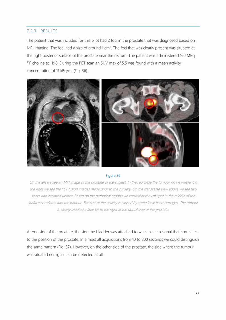
77
7.2.3 RESULTS
The patient that was included for this pilot had 2 foci in the prostate that was diagnosed based on
MRI imaging. The foci had a size of around 1 cm3. The foci that was clearly present was situated at
the right posterior surface of the prostate near the rectum. The patient was administered 160 MBq
18F choline at 11:18. During the PET scan an SUV max of 5.5 was found with a mean activity
concentration of 11 kBq/ml (Fig. 36).
Figure 36
On the left we see an MRI image of the prostate of the subject. In the red circle the tumour nr. I is visible. On
the right we see the PET fusion images made prior to the surgery. On the transverse view above we see two
spots with elevated uptake. Based on the patholical reports we know that the left spot in the middle of the
surface correlates with the tumour. The rest of the activity is caused by some local haemorrhages. The tumour
is clearly situated a little bit to the right at the dorsal side of the prostate.
At one side of the prostate, the side the bladder was attached to we can see a signal that correlates
to the position of the prostate. In almost all acquisitions from 10 to 300 seconds we could distinguish
the same pattern (Fig. 37). However, on the other side of the prostate, the side where the tumour
was situated no signal can be detected at all.

Figure 37
CLI images of the resected prostate. Above we see the images made of the more ventral side of the prostate
corresponding to images A from figure 38 and figure 39. On the left a raw image is shown from an acquisition
with a 300 second exposure time. Right of that 3 merged images of the light and processed CLI images are
shown for three different exposure times. A clear signal can be seen that correlates to the position of the
prostate. The lower three images are form the dorsal side of the prostate. They correlate to images B from
figure 38 and figure 39. Already in the raw image no signal can be detected. Also the processed merged
images show no signal but only some artefacts and a little bit of light leakage from the right were the door of
the cabinet is located.
7.2.4 DISCUSSION
We did see activity on the side imaged from position A (Fig. 39) but on the other side we did not
detect any activity at all. The places where we saw the activity was the side that was situated towards
the bladder. Based on the imaging the first lesion was situated at the other side near the rectum.
This was confirmed by pathological examination. The pathologist found 2 significant lesions. The
first lesion, lesion I corresponded with the lesion that was visible in the MRI and PET-CT scans.
Another lesion was found near the right seminal vesicle with ingrowth into the seminal vesicle. This is
lesion II in the images.
If we would have detected radioactivity from the tumour uptake it should have shown in image B
and then most likely at the marked areas. However, no signal was detected at this side at all. We can
thus conclude that we were not able to image the tumours within the prostate. Even though at
some places there was only a minimal surgical margin.
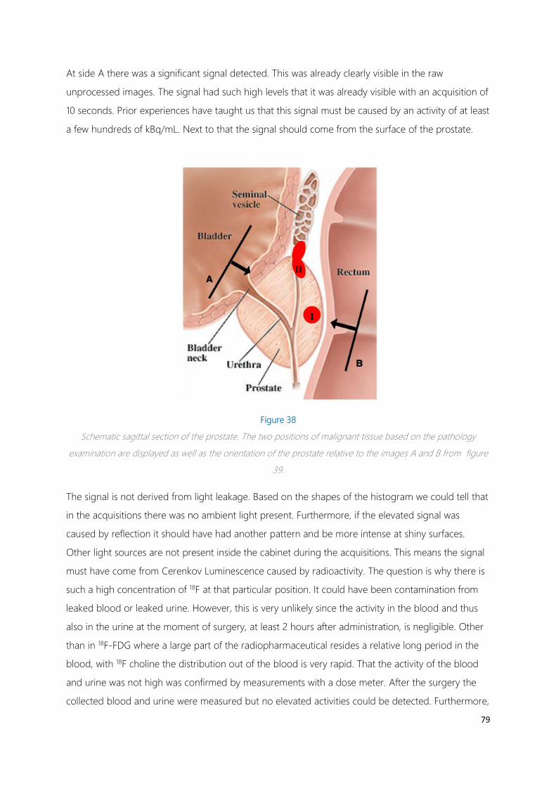
79
At side A there was a significant signal detected. This was already clearly visible in the raw
unprocessed images. The signal had such high levels that it was already visible with an acquisition of
10 seconds. Prior experiences have taught us that this signal must be caused by an activity of at least
a few hundreds of kBq/mL. Next to that the signal should come from the surface of the prostate.
Figure 38
Schematic sagittal section of the prostate. The two positions of malignant tissue based on the pathology
examination are displayed as well as the orientation of the prostate relative to the images A and B from figure
39.
The signal is not derived from light leakage. Based on the shapes of the histogram we could tell that
in the acquisitions there was no ambient light present. Furthermore, if the elevated signal was
caused by reflection it should have had another pattern and be more intense at shiny surfaces.
Other light sources are not present inside the cabinet during the acquisitions. This means the signal
must have come from Cerenkov Luminescence caused by radioactivity. The question is why there is
such a high concentration of 18F at that particular position. It could have been contamination from
leaked blood or leaked urine. However, this is very unlikely since the activity in the blood and thus
also in the urine at the moment of surgery, at least 2 hours after administration, is negligible. Other
than in 18F-FDG where a large part of the radiopharmaceutical resides a relative long period in the
blood, with 18F choline the distribution out of the blood is very rapid. That the activity of the blood
and urine was not high was confirmed by measurements with a dose meter. After the surgery the
collected blood and urine were measured but no elevated activities could be detected. Furthermore,
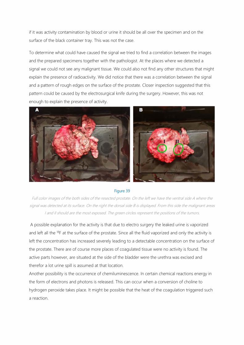
if it was activity contamination by blood or urine it should be all over the specimen and on the
surface of the black container tray. This was not the case.
To determine what could have caused the signal we tried to find a correlation between the images
and the prepared specimens together with the pathologist. At the places where we detected a
signal we could not see any malignant tissue. We could also not find any other structures that might
explain the presence of radioactivity. We did notice that there was a correlation between the signal
and a pattern of rough edges on the surface of the prostate. Closer inspection suggested that this
pattern could be caused by the electrosurgical knife during the surgery. However, this was not
enough to explain the presence of activity.
Figure 39
Full color images of the both sides of the resected prostate. On the left we have the ventral side A where the
signal was detected at its surface. On the right the dorsal side B is displayed. From this side the malignant areas
I and II should are the most exposed. The green circles represent the positions of the tumors.
A possible explanation for the activity is that due to electro surgery the leaked urine is vaporized
and left all the 18F at the surface of the prostate. Since all the fluid vaporized and only the activity is
left the concentration has increased severely leading to a detectable concentration on the surface of
the prostate. There are of course more places of coagulated tissue were no activity is found. The
active parts however, are situated at the side of the bladder were the urethra was excised and
therefor a lot urine spill is assumed at that location.
Another possibility is the occurrence of chemiluminescence. In certain chemical reactions energy in
the form of electrons and photons is released. This can occur when a conversion of choline to
hydrogen peroxide takes place. It might be possible that the heat of the coagulation triggered such
a reaction.

81
8 RADIATION SAFETY
As we learned Cerenkov imaging is dependent on radioactive sources. Since we are looking into an
intraoperative use we want to use the technique in patients. This requires a lot of activity that has to
be administered to those patients. The administered doses have to be at least equal to the amounts
that are used in PET imaging. As mentioned earlier this such an activity cannot indiscriminately be
administered. Although it is not a big issue for that particular patient. The patient can receive this
dose since it is of use for his clinical care and there will be more benefit then it does harm. However,
for the personnel that is involved in the administration, imaging, transport and surgery of this
patient this naturally does not apply. All the persons will receive a dose via the radioactive patient
and for them it can only do harm. The should keep the received dose as low as reasonably possible
conform the ALARA (As Low as Reasonably Achievable) principle. The workers on the nuclear
medicine department are specially trained to deal with radioactivity and can receive an excepted
annual dose. The bottleneck is the OR personnel. They are not specially trained as a radioactive
worker are limited to low annual dose while at the same time they have to stand next to the
radioactive patients throughout the entire surgery which will result in a high dose. Depending on the
dose they receive per surgery they are restricted to a certain number of these types of surgery a
year. If a surgeon cannot perform a certain amount of surgeries a year the technique will not be
valuable enough. The surgeon is not able to specialize in and optimize the surgery and relatively
little patients can be treated with a new invested technique.
The dose a surgeon will receive during a surgery with a radioactive patient is thus an important
parameter for the success of CLI.
8.1 RADIATION REGULATION
The protection of people against radiation in the Netherlands is regulated conform the
‘kernenergiewet’ and the ‘besluit stralingsbescherming’. In these laws dose limits are
described for all employees. These limits are defined as the annual effective dose a person can
receive. This is not a measurable variable but it can be calculated from different other physical
parameters and weigh factors as stipulated in directive ICRP 60. It is a measure for the amount of
radiation that is received by the whole body corrected for the type and energy of radiation and the
amount of damage it can do to any part of the body. It is measured in Sievert. The naturally
received background dose in the Netherlands for any person is 2.5 mSv/year. This is derived from
naturally present radon and radiation from space. The dose limits set by the ‘kernenergiewet’ are
defined as the annual dose that is received from ionizing radiation and artificial radiation sources in
addition to the background radiation. There are different categories of dose limits for employees:
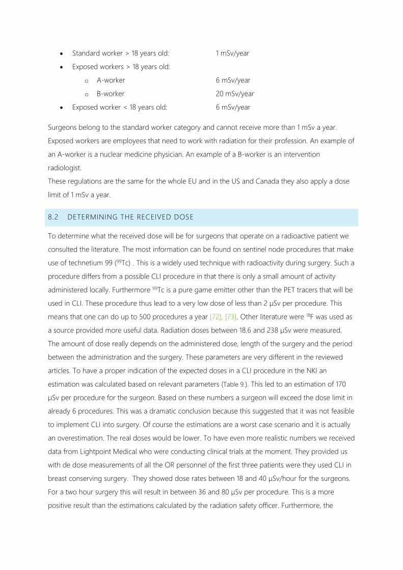
• Standard worker > 18 years old: 1 mSv/year
• Exposed workers > 18 years old:
o A-worker 6 mSv/year
o B-worker 20 mSv/year
• Exposed worker < 18 years old: 6 mSv/year
Surgeons belong to the standard worker category and cannot receive more than 1 mSv a year.
Exposed workers are employees that need to work with radiation for their profession. An example of
an A-worker is a nuclear medicine physician. An example of a B-worker is an intervention
radiologist.
These regulations are the same for the whole EU and in the US and Canada they also apply a dose
limit of 1 mSv a year.
8.2 DETERMINING THE RECEIVED DOSE
To determine what the received dose will be for surgeons that operate on a radioactive patient we
consulted the literature. The most information can be found on sentinel node procedures that make
use of technetium 99 (99Tc) . This is a widely used technique with radioactivity during surgery. Such a
procedure differs from a possible CLI procedure in that there is only a small amount of activity
administered locally. Furthermore 99Tc is a pure game emitter other than the PET tracers that will be
used in CLI. These procedure thus lead to a very low dose of less than 2 µSv per procedure. This
means that one can do up to 500 procedures a year [72], [73]. Other literature were 18F was used as
a source provided more useful data. Radiation doses between 18.6 and 238 µSv were measured.
The amount of dose really depends on the administered dose, length of the surgery and the period
between the administration and the surgery. These parameters are very different in the reviewed
articles. To have a proper indication of the expected doses in a CLI procedure in the NKI an
estimation was calculated based on relevant parameters (Table 9.). This led to an estimation of 170
µSv per procedure for the surgeon. Based on these numbers a surgeon will exceed the dose limit in
already 6 procedures. This was a dramatic conclusion because this suggested that it was not feasible
to implement CLI into surgery. Of course the estimations are a worst case scenario and it is actually
an overestimation. The real doses would be lower. To have even more realistic numbers we received
data from Lightpoint Medical who were conducting clinical trials at the moment. They provided us
with de dose measurements of all the OR personnel of the first three patients were they used CLI in
breast conserving surgery. They showed dose rates between 18 and 40 µSv/hour for the surgeons.
For a two hour surgery this will result in between 36 and 80 µSv per procedure. This is a more
positive result than the estimations calculated by the radiation safety officer. Furthermore, the

83
administered dose they used was 5 MBq/kg which is twice as high as the doses we use in the NKI.
The actual doses thus will probably be significantly lower. To give a more precise estimation of what
the received dose for a surgeon in the NKI will be we performed dose measurements on patients at
the nuclear department who were administered with clinical doses of 18F-FDG and 68Ga-Dotatate.
We also wanted to know what the received dose will be directly at the surface of a patient.
Table 9
Overview of a literature study into the received dose to surgeons when performing surgery on a radioactive
patient. The first two studies show the results for Tc99 which is used in sentinel node procedures. Next 5
different studies that have published received doses due to patients administered with 18F. The last row shows
the calculated estimation done by the radiation safety officer for a plausible scenario.
8.2.1 METHODS
We have measured patients who received clinical doses of 18F-FDG and 68Ga-Dotatate in the context
of a PET-CT scan. We measured the dose tempo with a dosimeter. We have measured on the
surface of the patients on the right and left flank in between the hip bone and the ribs and from the
front 30 cm from the bellybutton. The measurements were done prior to the PET-scan and directly
after the PET study.
The data will be plotted against the time obtain a curve that represents the dose flux for any time
after the administration of the radioactivity. This will be done for the three different measurement
positions and for both the 68Ga and the 18F.
8.2.2 RESULTS
We have measured seven patients who were administered with 68Ga and 10 patients who received
18F-FDG. In all the patients we measured twice on each position. Once prior to the scan and once
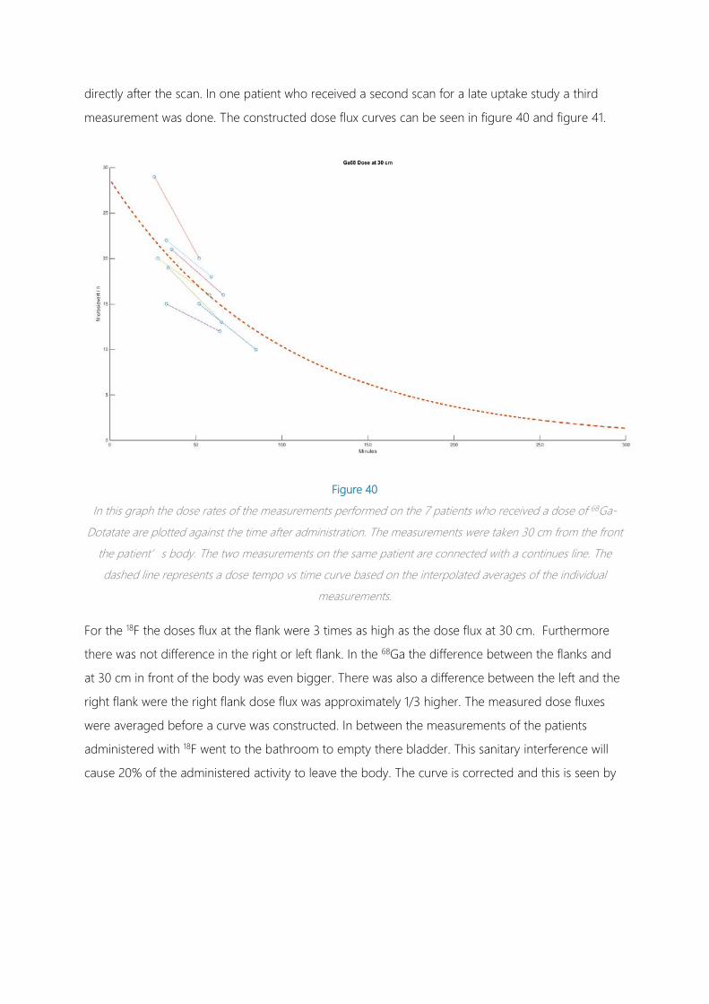
directly after the scan. In one patient who received a second scan for a late uptake study a third
measurement was done. The constructed dose flux curves can be seen in figure 40 and figure 41.
Figure 40
In this graph the dose rates of the measurements performed on the 7 patients who received a dose of 68Ga-
Dotatate are plotted against the time after administration. The measurements were taken 30 cm from the front
the patient’s body. The two measurements on the same patient are connected with a continues line. The
dashed line represents a dose tempo vs time curve based on the interpolated averages of the individual
measurements.
For the 18F the doses flux at the flank were 3 times as high as the dose flux at 30 cm. Furthermore
there was not difference in the right or left flank. In the 68Ga the difference between the flanks and
at 30 cm in front of the body was even bigger. There was also a difference between the left and the
right flank were the right flank dose flux was approximately 1/3 higher. The measured dose fluxes
were averaged before a curve was constructed. In between the measurements of the patients
administered with 18F went to the bathroom to empty there bladder. This sanitary interference will
cause 20% of the administered activity to leave the body. The curve is corrected and this is seen by
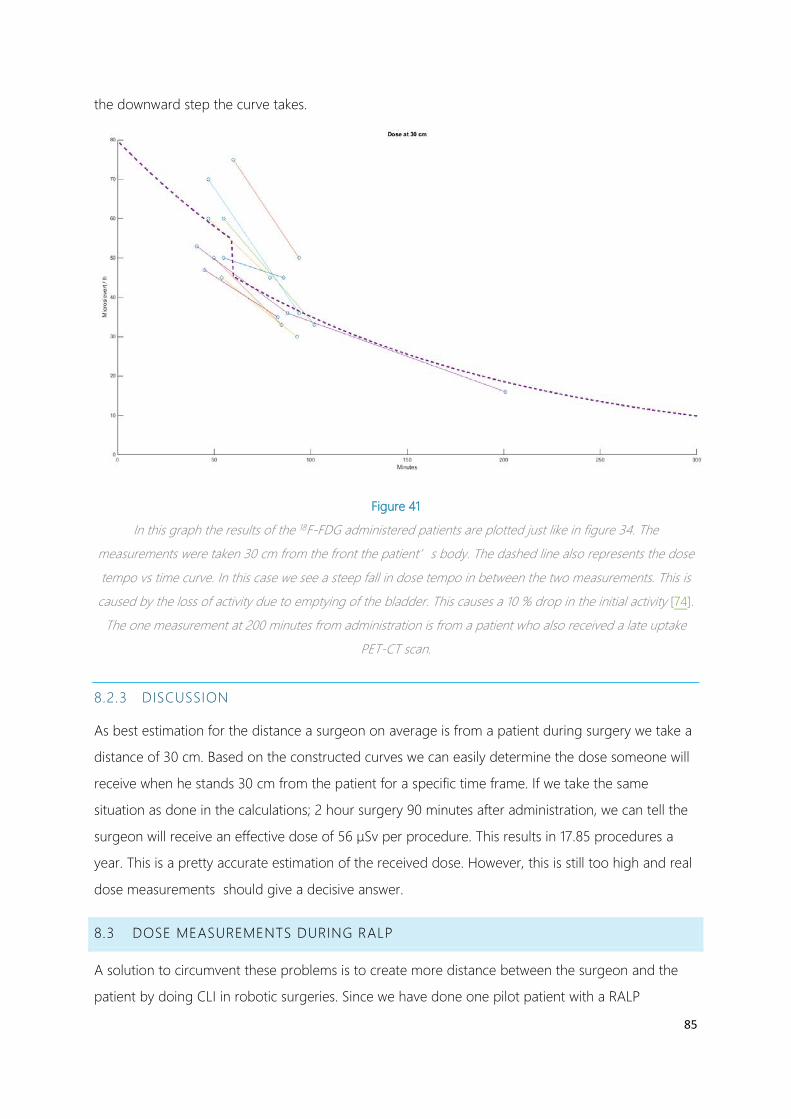
85
the downward step the curve takes.
Figure 41
In this graph the results of the 18F-FDG administered patients are plotted just like in figure 34. The
measurements were taken 30 cm from the front the patient’s body. The dashed line also represents the dose
tempo vs time curve. In this case we see a steep fall in dose tempo in between the two measurements. This is
caused by the loss of activity due to emptying of the bladder. This causes a 10 % drop in the initial activity [74].
The one measurement at 200 minutes from administration is from a patient who also received a late uptake
PET-CT scan.
8.2.3 DISCUSSION
As best estimation for the distance a surgeon on average is from a patient during surgery we take a
distance of 30 cm. Based on the constructed curves we can easily determine the dose someone will
receive when he stands 30 cm from the patient for a specific time frame. If we take the same
situation as done in the calculations; 2 hour surgery 90 minutes after administration, we can tell the
surgeon will receive an effective dose of 56 µSv per procedure. This results in 17.85 procedures a
year. This is a pretty accurate estimation of the received dose. However, this is still too high and real
dose measurements should give a decisive answer.
8.3 DOSE MEASUREMENTS DURING RALP
A solution to circumvent these problems is to create more distance between the surgeon and the
patient by doing CLI in robotic surgeries. Since we have done one pilot patient with a RALP
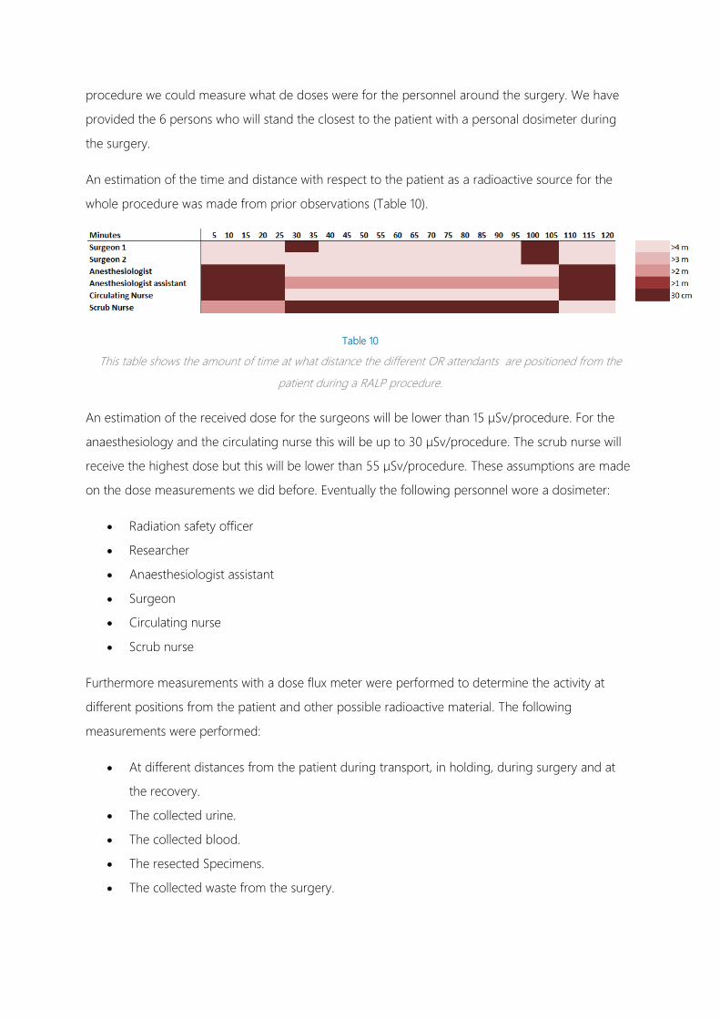
procedure we could measure what de doses were for the personnel around the surgery. We have
provided the 6 persons who will stand the closest to the patient with a personal dosimeter during
the surgery.
An estimation of the time and distance with respect to the patient as a radioactive source for the
whole procedure was made from prior observations (Table 10).
Table 10
This table shows the amount of time at what distance the different OR attendants are positioned from the
patient during a RALP procedure.
An estimation of the received dose for the surgeons will be lower than 15 µSv/procedure. For the
anaesthesiology and the circulating nurse this will be up to 30 µSv/procedure. The scrub nurse will
receive the highest dose but this will be lower than 55 µSv/procedure. These assumptions are made
on the dose measurements we did before. Eventually the following personnel wore a dosimeter:
• Radiation safety officer
• Researcher
• Anaesthesiologist assistant
• Surgeon
• Circulating nurse
• Scrub nurse
Furthermore measurements with a dose flux meter were performed to determine the activity at
different positions from the patient and other possible radioactive material. The following
measurements were performed:
• At different distances from the patient during transport, in holding, during surgery and at
the recovery.
• The collected urine.
• The collected blood.
• The resected Specimens.
• The collected waste from the surgery.

87
8.3.1 RESULTS
The patient was administered at 11:18 with 160 MBq 18F-FDG. The surgery started at 12:30 and ended
at 14:35. In this time span the surgeon received a dose of 7 µSv. The highest dose was received by
the scrub nurse who has to stand next to the patient for almost the whole procedure. She received a
dose of 22 µSv. This means that the surgeon can perform 142 such procedures a year based on
these measurements (Table 11). The scrub nurse however, is the limiting factor with 45 procedures a
year. This is already a lot more than was earlier determined for a standard operating procedure
without robotic assistance.
Table 11
The doses measured with the personal dosimeters during the RALP procedure. The dose is given in micro
Sievert. In the right column the amount of procedures per year that can be performed based on these doses is
given
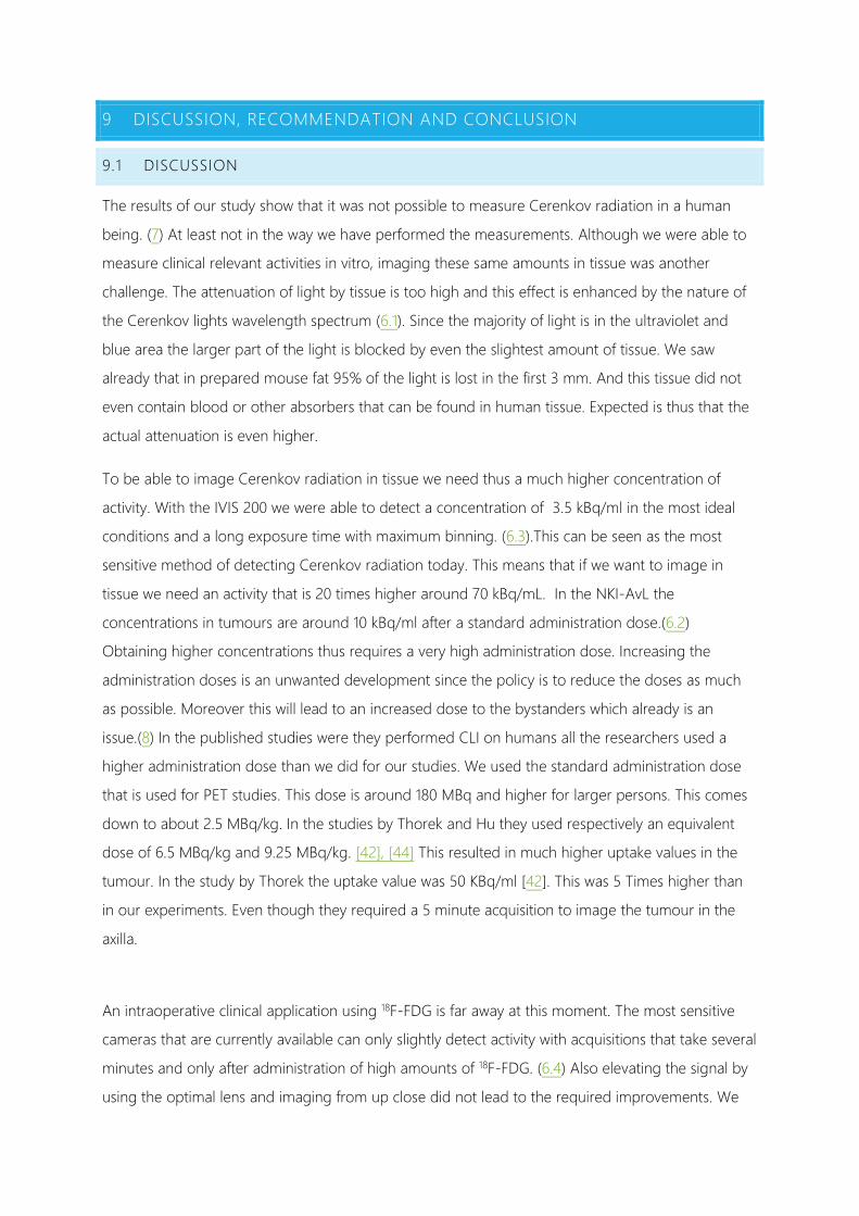
9 DISCUSSION, RECOMMENDATION AND CONCLUSION
9.1 DISCUSSION
The results of our study show that it was not possible to measure Cerenkov radiation in a human
being. (7) At least not in the way we have performed the measurements. Although we were able to
measure clinical relevant activities in vitro, imaging these same amounts in tissue was another
challenge. The attenuation of light by tissue is too high and this effect is enhanced by the nature of
the Cerenkov lights wavelength spectrum (6.1). Since the majority of light is in the ultraviolet and
blue area the larger part of the light is blocked by even the slightest amount of tissue. We saw
already that in prepared mouse fat 95% of the light is lost in the first 3 mm. And this tissue did not
even contain blood or other absorbers that can be found in human tissue. Expected is thus that the
actual attenuation is even higher.
To be able to image Cerenkov radiation in tissue we need thus a much higher concentration of
activity. With the IVIS 200 we were able to detect a concentration of 3.5 kBq/ml in the most ideal
conditions and a long exposure time with maximum binning. (6.3).This can be seen as the most
sensitive method of detecting Cerenkov radiation today. This means that if we want to image in
tissue we need an activity that is 20 times higher around 70 kBq/mL. In the NKI-AvL the
concentrations in tumours are around 10 kBq/ml after a standard administration dose.(6.2)
Obtaining higher concentrations thus requires a very high administration dose. Increasing the
administration doses is an unwanted development since the policy is to reduce the doses as much
as possible. Moreover this will lead to an increased dose to the bystanders which already is an
issue.(8) In the published studies were they performed CLI on humans all the researchers used a
higher administration dose than we did for our studies. We used the standard administration dose
that is used for PET studies. This dose is around 180 MBq and higher for larger persons. This comes
down to about 2.5 MBq/kg. In the studies by Thorek and Hu they used respectively an equivalent
dose of 6.5 MBq/kg and 9.25 MBq/kg. [42], [44] This resulted in much higher uptake values in the
tumour. In the study by Thorek the uptake value was 50 KBq/ml [42]. This was 5 Times higher than
in our experiments. Even though they required a 5 minute acquisition to image the tumour in the
axilla.
An intraoperative clinical application using 18F-FDG is far away at this moment. The most sensitive
cameras that are currently available can only slightly detect activity with acquisitions that take several
minutes and only after administration of high amounts of 18F-FDG. (6.4) Also elevating the signal by
using the optimal lens and imaging from up close did not lead to the required improvements. We

89
were able to improve the images by using more sophisticated acquisitions and by image processing.
However, for image guided surgery this is not sufficient enough. For this purpose we want to have
fast acquisitions that are near real time with a clear signal to background ratio and a high a
resolution.
Besides the problems we have with the sensitivity the ambient light forms a problem. In a system
such as the IVIS 200 that are designed for small animals or specimens it is not difficult to eliminate
all the light. In this case you build a cabinet with light tight materials and a perfect seal to close the
door. Of course you are able to build such a design on a larger scale that will fit humans. It is of
course not very patient friendly to put patients in a dark box. Also in a surgical setting this is not an
option. Another option is that you are able to make the whole OR dark. In practice this is very
difficult since any small LED on any device should be eliminated because any spec of light can
disturb the measurements. Furthermore, temporarily eliminating all the light in the OR seems like a
bad idea when a whole OR team is present with all kinds of equipment that keep the patient alive
that have to be constantly monitored. The best option is to try to seal of only a small area of the
patient that you want to image. However, it will not be easy to come up with a design that can give
a light tight seal between the lens and any part of the patient that meets the quality standards for
sterile OR equipment. Such a system is currently under development by Lightpoint Medical from the
UK. Another option to eliminate light is to use the technique during scopic procedures. In this case
you bring the lens of the camera inside the patient's body. Turning of the light inside the body can
be harmlessly done. However, it is not really clear if there will be no light at all. When performing
scopic surgery on the abdomen a thin skin might transmit some of the light from the OR room. Next
to that the holes that provide the entrance of the scope and other equipment should be sealed of
light tight.
Image guided surgery using 18F-FDG is currently not feasible. In order to make such an application
useful a large tumour to background ratio, a high signal and a sensitive system are required to be
able to detect malignant tissue in near time and behind a layer of tissue. The Cerenkov radiation
derived from 18F-FDG is able to provide a good tumour to background ratio in the same way as it
does with PET imaging. The intensity of the signal or the sensitivity of the imaging equipment is the
limiting factor. To meet the demands for image guided surgery several orders of magnitude in
sensitivity have to be gained.
9.2 RECOMMENDATIONS
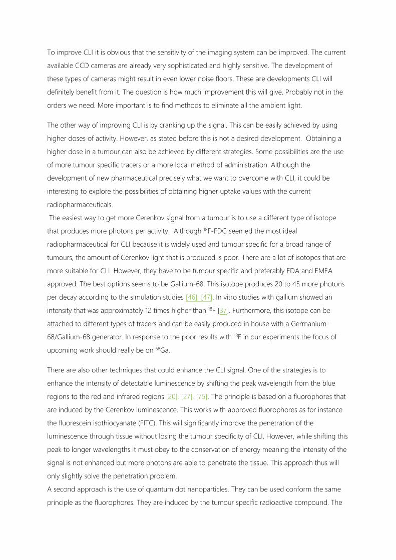
To improve CLI it is obvious that the sensitivity of the imaging system can be improved. The current
available CCD cameras are already very sophisticated and highly sensitive. The development of
these types of cameras might result in even lower noise floors. These are developments CLI will
definitely benefit from it. The question is how much improvement this will give. Probably not in the
orders we need. More important is to find methods to eliminate all the ambient light.
The other way of improving CLI is by cranking up the signal. This can be easily achieved by using
higher doses of activity. However, as stated before this is not a desired development. Obtaining a
higher dose in a tumour can also be achieved by different strategies. Some possibilities are the use
of more tumour specific tracers or a more local method of administration. Although the
development of new pharmaceutical precisely what we want to overcome with CLI, it could be
interesting to explore the possibilities of obtaining higher uptake values with the current
radiopharmaceuticals.
The easiest way to get more Cerenkov signal from a tumour is to use a different type of isotope
that produces more photons per activity. Although 18F-FDG seemed the most ideal
radiopharmaceutical for CLI because it is widely used and tumour specific for a broad range of
tumours, the amount of Cerenkov light that is produced is poor. There are a lot of isotopes that are
more suitable for CLI. However, they have to be tumour specific and preferably FDA and EMEA
approved. The best options seems to be Gallium-68. This isotope produces 20 to 45 more photons
per decay according to the simulation studies [46], [47]. In vitro studies with gallium showed an
intensity that was approximately 12 times higher than 18F [37]. Furthermore, this isotope can be
attached to different types of tracers and can be easily produced in house with a Germanium-
68/Gallium-68 generator. In response to the poor results with 18F in our experiments the focus of
upcoming work should really be on 68Ga.
There are also other techniques that could enhance the CLI signal. One of the strategies is to
enhance the intensity of detectable luminescence by shifting the peak wavelength from the blue
regions to the red and infrared regions [20], [27], [75]. The principle is based on a fluorophores that
are induced by the Cerenkov luminescence. This works with approved fluorophores as for instance
the fluorescein isothiocyanate (FITC). This will significantly improve the penetration of the
luminescence through tissue without losing the tumour specificity of CLI. However, while shifting this
peak to longer wavelengths it must obey to the conservation of energy meaning the intensity of the
signal is not enhanced but more photons are able to penetrate the tissue. This approach thus will
only slightly solve the penetration problem.
A second approach is the use of quantum dot nanoparticles. They can be used conform the same
principle as the fluorophores. They are induced by the tumour specific radioactive compound. The

91
difference with these nanoparticles is that depending on their design can be induced by photons or
gamma radiation [70], [76]. The most promising part is that they possess high quantum yields and
thus can deliver a very high intensity. Mice studies have shown a 50 fold increase in sensitivity in vivo
[70]. The downside here is that most quantum dot nanoparticles are cytotoxic and although new
more biocompatible approaches are being developed quantum dots are far from approval for
clinical use [62].
CLI for image guided oncology surgery seems to be far from achievable. There are more
opportunities for other intraoperative applications. A possible application is on site margin
detection. The immediate knowledge on the surgical margins can be very valuable. Such an
application solves already a large part of the difficulties that are presented for image guidance. First
of all it can take place ex vivo and thus in a specialized cabinet where all ambient light can be
blocked. Furthermore we don’t need near real time speed. For an application like this a five minute
acquisition will be no problem. Lastly you only want to look at the surface of the specimen. The lack
of penetration by the Cerenkov light would be beneficial for this purpose. An extension to this
technique could be to do in vivo margin detection. By imaging the resection area you might be able
to detect any residual malignant tissues. If you are able to image the whole resection area in one
acquisition this will not take much time but if any residue can be detected you directly know where
extra tissue should be removed.
9.3 CONCLUSION
Image guided surgery based on Cerenkov Imaging is theoretically very promising. However, the
reality is that the intensities of the signal are too weak to use for in vivo imaging during surgery.
Also, there are currently no possibilities to sufficiently enhance the signal besides the use of
tremendously high activities. In the quest for bringing CLI in the clinic further research should focus
on high emitting isotopes of which 68Ga seems to be the most logical choice. More specifically, to
bring CLI into the OR an application that focuses on perioperative margin detection is most likely to
succeed. A good starting point can be the margin detection of resected prostates. In this type of
surgery immediate knowledge of surgical margins is very relevant. Also the radiation safety issue can
be bypassed since most prostatectomy's are performed using the RALP procedure. To conclude, a
specific radiotracer for prostate cancer with 68Ga will be available in the near future.
10 BIBLIOGRAPHY
[1] R. Robertson, M. S. Germanos, C. Li, G. S. Mitchell, S. R. Cherry, and M. D. Silva,
“Optical imaging of Cerenkov light generation from positron-emitting
radiotracers.,” Phys. Med. Biol., vol. 54, no. 16, pp. N355–65, Aug. 2009.
[2] B. M. Bolotovskii, “Vavilov – Cherenkov radiation: its discovery and application,”
Physics-Uspekhi, vol. 52, no. 11, pp. 1099–1110, Nov. 2009.
[3] E. Curie and V. Sheean, Madame Curie. 1938.
[4] Pavel A. Cherenkov, “Radiation of Particles Moving at a Velocity Exceeding That of
Light, and Some of the Possibilities for Their Use in Experimental Physics,” Nobel
Lect. Phys. 1942-1962, p. 1964, 1964.
[5] P. a. Cherenkov, “Visible radiation produced by electrons moving in a medium with
velocities exceeding that of light [1],” Phys. Rev., vol. 52, pp. 378–379, 1937.
[6] J. V. Jelley, Cerenkov Radiation and its Applications. 1958.
[7] A. A. Watson, “The discovery of Cherenkov radiation and its use in the detection of
extensive air showers,” in Cosmic Ray International Seminar 2010, 2010, pp. 1–10.
[8] W. M. Burch, “Čerenkov Light from 32P, Burch.pdf,” Nature, vol. 234, p. 358, 1971.
[9] Pavel A. Cherenkov, “Radiation of Particles Moving at a Velocity Exceeding That of
Light, and Some of the Possibilities for Their Use in Experimental Physics,” Nobel
Lect. Phys. 1942-1962, pp. 426–440, 1964.
[10] F. Boschi, L. Calderan, D. D’Ambrosio, M. Marengo, A. Fenzi, R. Calandrino, A.
Sbarbati, and A. E. Spinelli, “In vivo 18F-FDG tumour uptake measurements in small
animals using Cerenkov radiation.,” Eur. J. Nucl. Med. Mol. Imaging, vol. 38, no. 1,
pp. 120–7, Jan. 2011.
[11] H. Liu, C. M. Carpenter, H. Jiang, G. Pratx, C. Sun, M. P. Buchin, S. S. Gambhir, L.
Xing, and Z. Cheng, “Intraoperative imaging of tumors using Cerenkov
luminescence endoscopy: a feasibility experimental study.,” J. Nucl. Med., vol. 53,
no. 10, pp. 1579–84, Oct. 2012.
93
[12] J. P. Holland, G. Normand, A. Ruggiero, and J. S. Lewis, “Intraoperative Imaging of
Positron Emission Tomographic Radiotracers Using Cerenkov Luminescence
Emissions,” Mol. Imaging Biol., vol. 10, no. 3, pp. 177–186, 2011.
[13] D. L. J. Thorek, D. S. Abou, B. J. Beattie, R. M. Bartlett, R. Huang, P. B. Zanzonico, and
J. Grimm, “Positron lymphography: multimodal, high-resolution, dynamic mapping
and resection of lymph nodes after intradermal injection of 18F-FDG.,” J. Nucl.
Med., vol. 53, no. 9, pp. 1438–45, Sep. 2012.
[14] S. Y. Jeong, M.-H. Hwang, J. E. Kim, S. Kang, J. C. Park, J. Yoo, J.-H. Ha, S.-W. Lee, B.-
C. Ahn, and J. Lee, “Combined Cerenkov luminescence and nuclear imaging of
radioiodine in the thyroid gland and thyroid cancer cells expressing sodium iodide
symporter: initial feasibility study.,” Endocr. J., vol. 58, no. 7, pp. 575–83, Jan. 2011.
[15] Y. Xu, E. Chang, H. Liu, H. Jiang, S. S. Gambhir, and Z. Cheng, “Proof-of-concept
study of monitoring cancer drug therapy with cerenkov luminescence imaging.,” J.
Nucl. Med., vol. 53, no. 2, pp. 312–7, Feb. 2012.
[16] C. Lohrmann, H. Zhang, D. L. Thorek, P. Desai, P. B. Zanzonico, J. a. O’Donoghue,
C. P. Irwin, T. Reiner, J. Grimm, and W. a. Weber, “Cerenkov luminescence imaging
for radiation dose calculation of a 90Y-labeled gastrin releasing peptide receptor
(GRPr) antagonist,” J. Nucl. Med., 2015.
[17] J. Czupryna, a. V. Kachur, E. Blankemeyer, a. V. Popov, a. D. Arroyo, J. S. Karp, and E.
J. Delikatny, “Cerenkov-Specific Contrast Agents for Detection of pH In Vivo,” J.
Nucl. Med., vol. 56, no. 215, pp. 483–488, 2015.
[18] S. Yamamoto, T. Toshito, K. Fujii, Y. Morishita, S. Okumura, and M. Komori, “High
resolution Cerenkov light imaging of induced positron distribution in proton
therapy,” Med. Phys., vol. 41, p. 111913, 2014.
[19] L. a Jarvis, R. Zhang, D. J. Gladstone, S. Jiang, W. Hitchcock, O. D. Friedman, A. K.
Glaser, M. Jermyn, and B. W. Pogue, “Cherenkov video imaging allows for the first
visualization of radiation therapy in real time.,” Int. J. Radiat. Oncol. Biol. Phys., vol.
89, no. 3, pp. 615–22, Jul. 2014.
[20] M. A. Lewis, V. D. Kodibagkar, O. K. Oz, and R. P. Mason, “On the potential for
molecular imaging with Cerenkov luminescence,” Opt. Lett., vol. 35, no. 23, pp.
3889–3891, 2011.
[21] C. Ran, Z. Zhang, J. Hooker, and A. Moore, “In vivo photoactivation without
‘light’: use of Cherenkov radiation to overcome the penetration limit of light.,”
Mol. Imaging Biol., vol. 14, no. 2, pp. 156–62, Apr. 2012.
[22] J. Grimm, “Cancer nanomedicine: Therapy from within,” Nat. Nanotechnol., vol. 10,
no. 4, pp. 299–300, 2015.
[23] O. Heaviside, “Electromagnetic effects of a moving charge,” Electr., p. 23, 1888.
[24] Lord Kelvin, “Philosophical Magazine,” Philos. Mag. J. Sci., vol. 2, no. 7, pp. 1–40,
1901.
[25] G. N. Afanasiev, Vavilov Cherenkov and Synchotron Radiation - Foundations and
applications. 2004, pp. 32–36.
[26] G. S. Mitchell, R. K. Gill, D. L. Boucher, C. Li, and S. R. Cherry, “In vivo Cerenkov
luminescence imaging: a new tool for molecular imaging.,” Philos. Trans. A. Math.
Phys. Eng. Sci., vol. 369, no. 1955, pp. 4605–19, Nov. 2011.
[27] X. Ma, J. Wang, and Z. Cheng, “Cerenkov radiation: a multi-functional approach for
biological sciences,” Front. Phys., vol. 2, no. February, pp. 1–14, 2014.
[28] “Measurement of beta emitting nuclides using cerenkov radiation, Ross 1969.” .
[29] A. E. Spinelli, D. D’Ambrosio, L. Calderan, M. Marengo, A. Sbarbati, and F. Boschi,
“Cerenkov radiation allows in vivo optical imaging of positron emitting
radiotracers.,” Phys. Med. Biol., vol. 55, no. 2, pp. 483–95, Jan. 2010.
[30] Y. Xu, H. Liu, and Z. Cheng, “Harnessing the power of radionuclides for optical
imaging: Cerenkov luminescence imaging.,” J. Nucl. Med., vol. 52, no. 12, pp. 2009–
18, Dec. 2011.
[31] D. L. J. Thorek, R. Robertson, W. A. Bacchus, J. Hahn, J. Rothberg, and J. Bradley,
“Cerenkov imaging - a new modality for molecular imaging,” vol. 2, no. 2, pp.
163–173, 2012.

95
[32] A. E. Spinelli, D. D’Ambrosio, L. Calderan, M. Marengo, A. Sbarbati, and F. Boschi,
“Optical Imaging of Positron Emitting Radiotracers,” Phys. Med. Biol., vol. 55, pp.
483–495, 2009.
[33] J. C. Park, G. Il An, S.-I. Park, J. Oh, H. J. Kim, Y. Su Ha, E. K. Wang, K. Min Kim, J. Y.
Kim, J. Lee, M. J. Welch, and J. Yoo, “Luminescence imaging using radionuclides: a
potential application in molecular imaging.,” Nucl. Med. Biol., vol. 38, no. 3, pp.
321–9, Apr. 2011.
[34] Z. Hu, J. Liang, W. Yang, W. Fan, C. Li, X. Ma, X. Chen, X. Ma, X. Li, X. Qu, J. Wang, F.
Cao, and J. Tian, “Experimental Cerenkov luminescence tomography of the mouse
model with SPECT imaging validation.,” Opt. Express, vol. 18, no. 24, pp. 24441–50,
Nov. 2010.
[35] J. S. Cho, R. Taschereau, S. Olma, K. Liu, Y.-C. Chen, C. K.-F. Shen, R. M. van Dam,
and A. F. Chatziioannou, “Cerenkov radiation imaging as a method for quantitative
measurements of beta particles in a microfluidic chip.,” Phys. Med. Biol., vol. 54, no.
22, pp. 6757–71, Nov. 2009.
[36] N. L. Ackerman and E. E. Graves, “The potential for Cerenkov luminescence
imaging of alpha-emitting radionuclides.,” Phys. Med. Biol., vol. 57, no. 3, pp. 771–
83, Feb. 2012.
[37] J. D. Steinberg, A. Raju, P. Chandrasekharan, C.-T. Yang, K. Khoo, J.-P. Abastado, E.
G. Robins, and D. W. Townsend, “Negative contrast Cerenkov luminescence
imaging of blood vessels in a tumor mouse model using [68Ga]gallium chloride.,”
EJNMMI Res., vol. 4, no. 1, p. 15, Jan. 2014.
[38] D. L. J. Thorek, S. Das, and J. Grimm, “Molecular Imaging Using Nanoparticle
Quenchers of Cerenkov Luminescence.,” Small, vol. 7, no. 33, pp. 1–6, May 2014.
[39] A. Ruggiero, J. P. Holland, J. S. Lewis, and J. Grimm, “Cerenkov luminescence
imaging of medical isotopes.,” J. Nucl. Med., vol. 51, no. 7, pp. 1123–30, Jul. 2010.
[40] P. T. K. Chin, M. M. Welling, S. C. J. Meskers, R. a Valdes Olmos, H. Tanke, and F. W.
B. van Leeuwen, “Optical imaging as an expansion of nuclear medicine: Cerenkov-
based luminescence vs fluorescence-based luminescence.,” Eur. J. Nucl. Med. Mol.
Imaging, vol. 40, no. 8, pp. 1283–91, Aug. 2013.

[41] A. E. Spinelli, M. Ferdeghini, C. Cavedon, E. Zivelonghi, R. Calandrino, A. Fenzi, A.
Sbarbati, and F. Boschi, “First human Cerenkography.,” J. Biomed. Opt., vol. 18, no.
2, p. 20502, Feb. 2013.
[42] D. L. J. Thorek, C. C. Riedl, and J. Grimm, “Clinical Cerenkov luminescence imaging
of (18)F-FDG.,” J. Nucl. Med., vol. 55, no. 1, pp. 95–8, Jan. 2014.
[43] D. L. J. Thorek, C. C. Riedl, and J. Grimm, “Reply: Human Cerenkov imaging using
18F-FDG.,” J. Nucl. Med., vol. 55, no. 3, pp. 523–4, Mar. 2014.
[44] H. Hu, X. Cao, F. Kang, M. Wang, Y. Lin, M. Liu, S. Li, L. Yao, J. Liang, J. Liang, Y. Nie,
X. Chen, J. Wang, and K. Wu, “Feasibility study of novel endoscopic Cerenkov
luminescence imaging system in detecting and quantifying gastrointestinal disease:
first human results,” Eur. Radiol., 2015.
[45] H. Liu, X. Zhang, B. Xing, P. Han, S. S. Gambhir, and Z. Cheng, “Radiation-
luminescence-excited quantum dots for in vivo multiplexed optical imaging,” Small,
vol. 6, pp. 1087–1091, 2010.
[46] B. J. Beattie, D. L. J. Thorek, C. R. Schmidtlein, K. S. Pentlow, J. L. Humm, and A. H.
Hielscher, “Quantitative modeling of Cerenkov light production efficiency from
medical radionuclides,” PLoS One, vol. 7, no. 2, 2012.
[47] R. K. Gill, G. S. Mitchell, and S. R. Cherry, “Computed Cerenkov luminescence yields
for radionuclides used in biology and medicine,” Phys. Med. Biol., vol. 60, pp.
4263–4280, 2015.
[48] R. G. Pleijhuis, M. Graafland, J. de Vries, J. Bart, J. S. de Jong, and G. M. van Dam,
“Obtaining adequate surgical margins in breast-conserving therapy for patients
with early-stage breast cancer: current modalities and future directions.,” Ann. Surg.
Oncol., vol. 16, no. 10, pp. 2717–30, Oct. 2009.
[49] L. Tafra, R. Fine, P. Whitworth, M. Berry, J. Woods, G. Ekbom, J. Gass, P. Beitsch, D.
Dodge, L. Han, T. Potruch, D. Francescatti, L. Oetting, J. S. Smith, H. Snider, D.
Kleban, A. Chagpar, and S. Akbari, “Prospective randomized study comparing cryo-
assisted and needle-wire localization of ultrasound-visible breast tumors,” Am. J.
Surg., vol. 192, pp. 462–470, 2006.
97
[50] I. C. Bennett, J. Greenslade, and H. Chiam, “Intraoperative ultrasound-guided
excision of nonpalpable breast lesions,” World J. Surg., vol. 29, pp. 369–374, 2005.
[51] S. M. Evans, J. L. Millar, M. Frydenberg, D. G. Murphy, I. D. Davis, T. Spelman, D. M.
Bolton, G. G. Giles, J. Dean, A. J. Costello, A. G. Frauman, P. a Kearns, L. Day, C.
Daniels, and J. J. McNeil, “Positive surgical margins: rate, contributing factors and
impact on further treatment: findings from the Prostate Cancer Registry.,” BJU Int.,
pp. 1–11, Oct. 2013.
[52] A. Tewari, P. Sooriakumaran, D. a Bloch, U. Seshadri-Kreaden, A. E. Hebert, and P.
Wiklund, “Positive surgical margin and perioperative complication rates of primary
surgical treatments for prostate cancer: a systematic review and meta-analysis
comparing retropubic, laparoscopic, and robotic prostatectomy.,” Eur. Urol., vol. 62,
no. 1, pp. 1–15, Jul. 2012.
[53] I. D. Nagtegaal and P. Quirke, “What is the role for the circumferential margin in
the modern treatment of rectal cancer?,” J. Clin. Oncol., vol. 26, no. 2, pp. 303–312,
2008.
[54] V. S. Klimberg, S. Harms, and S. Korourian, “Assessing margin status,” Surg.
Oncol., vol. 8, no. 1999, pp. 77–84, 1999.
[55] P. Swindle, J. a Eastham, M. Ohori, M. W. Kattan, T. Wheeler, N. Maru, K. Slawin, and
P. T. Scardino, “Do margins matter? The prognostic significance of positive surgical
margins in radical prostatectomy specimens.,” J. Urol., vol. 174, no. 3, pp. 903–7,
Sep. 2005.
[56] A. Binahmed, R. W. Nason, and A. a Abdoh, “The clinical significance of the positive
surgical margin in oral cancer.,” Oral Oncol., vol. 43, no. 8, pp. 780–4, Sep. 2007.
[57] N. Houssami, P. MacAskill, M. L. Marinovich, J. M. Dixon, L. Irwig, M. E. Brennan, and
L. J. Solin, “Meta-analysis of the impact of surgical margins on local recurrence in
women with early-stage invasive breast cancer treated with breast-conserving
therapy,” Eur. J. Cancer, vol. 46, no. 18, pp. 3219–3232, 2010.
[58] C. H. Lee and D. Carter, “Detecting residual tumor after excisional biopsy of
impalpable breast carcinoma: Efficacy of comparing preoperative mammograms

with radiographs of the biopsy specimen,” Am. J. Roentgenol., vol. 164, pp. 81–86,
1995.
[59] T. Tsuboi, M. Ohori, K. Kuroiwa, V. E. Reuter, M. W. Kattan, J. a. Eastham, and P. T.
Scardino, “Is intraoperative frozen section analysis an efficient way to reduce
positive surgical margins?,” Urology, vol. 66, no. 6, pp. 1287–1291, 2005.
[60] M. Bakhshandeh, O. S. Tutuncuoglu, G. Fischer, and S. Masood, “Use of Imprint
Cytology for Assessment of Surgical Margins in Lumpectomy Specimens of Breast
Cancer Patients,” Diagn. Cytopathol., vol. 35, no. 10, pp. 525–528, 2007.
[61] P. M. Lane, T. Gilhuly, P. Whitehead, H. Zeng, C. F. Poh, S. Ng, P. M. Williams, L.
Zhang, M. P. Rosin, and C. E. MacAulay, “Simple device for the direct visualization
of oral-cavity tissue fluorescence.,” J. Biomed. Opt., vol. 11, no. 2, p. 024006, 2006.
[62] S. Keereweer, J. D. F. Kerrebijn, P. B. a a van Driel, B. Xie, E. L. Kaijzel, T. J. a Snoeks, I.
Que, M. Hutteman, J. R. van der Vorst, J. S. D. Mieog, A. L. Vahrmeijer, C. J. H. van
de Velde, R. J. Baatenburg de Jong, and C. W. G. M. Löwik, “Optical image-guided
surgery--where do we stand?,” Mol. Imaging Biol., vol. 13, no. 2, pp. 199–207, Apr.
2011.
[63] D. Hanahan and R. A. Weinberg, “Hallmarks of cancer: The next generation,” Cell,
vol. 144, no. 5. pp. 646–674, 2011.
[64] T. J. a Snoeks, P. B. a a Van Driel, S. Keereweer, S. Aime, K. M. Brindle, G. M. Van
Dam, C. W. G. M. Löwik, V. Ntziachristos, and a. L. Vahrmeijer, “Towards a
successful clinical implementation of fluorescence-guided surgery,” Mol. Imaging
Biol., vol. 16, no. November 2013, pp. 147–151, 2014.
[65] T. G. Phan and A. Bullen, “Practical intravital two-photon microscopy for
immunological research: faster, brighter, deeper.,” Immunol. Cell Biol., vol. 88, no.
4, pp. 438–444, 2010.
[66] H. Liu, G. Ren, Z. Miao, X. Zhang, X. Tang, P. Han, S. S. Gambhir, and Z. Cheng,
“Molecular optical imaging with radioactive probes.,” PLoS One, vol. 5, no. 3, p.
e9470, Jan. 2010.
[67] D. J. Denvir and E. Conroy, “Electron-multiplying CCD: the new ICCD,” Proc. SPIE,
vol. 4796, no. Cic, pp. 164–174, 2003.
99
[68] D. Dussault and P. Hoess, “Noise performance comparison of ICCD with CCD and
EMCCD cameras,” Proc. SPIE, vol. 5563, pp. 195–204, 2004.
[69] L. Kuster, “Feasibility study of Cerenkov Luminescence Imaging for Clinical
Applications,” 2014.
[70] X. Cao, X. Chen, F. Kang, X. Cao, Y. Zhan, J. Wang, K. Wu, and J. Liang, “Sensitivity
improvement of Cerenkov luminescence endoscope with terbium doped Gd2O2S
nanoparticles,” Appl. Phys. Lett., vol. 106, p. 213702, 2015.
[71] C. Sachpekidis, A. Afshar-Oromieh, M. Roethke, H.-P. Schlemmer, U. Haberkorn, and
A. Dimitrakopoulou-Strauss, “68Ga-PSMA dynamic PET/CT imaging of prostate
cancer: Tracer distribution patterns and pharmacokinetics,” J. Nucl. Med., vol. 56,
no. supplement_3, p. 397–, May 2015.
[72] M. Keshtgar, W. Waddington, Lakhani, and P. Ell, “The Sentinel Node in Surgical
Oncology.” pp. 98–99, 1999.
[73] M. Giuliano, A. E. Giuliiano, and W. H. Strauss, Radioguided Surgery - A
comprehensive team approach. 2008, p. 41.
[74] T. Bach-Gansmo, J. Dybvik, T. Adamsen, and A. Naum, “Variation in urinary
excretion of FDG, yet another uncertainty in quantitative PET.,” Acta Radiol. short
reports, vol. 1, no. 8, p. 26, Jan. 2012.
[75] D. L. J. Thorek, A. Ogirala, B. J. Beattie, and J. Grimm, “Quantitative imaging of
disease signatures through radioactive decay signal conversion.,” Nat. Med., vol. 19,
no. January, pp. 1345–50, 2013.
[76] W. Guo, X. Sun, O. Jacobson, X. Yan, K. Min, A. Srivatsan, G. Niu, D. O. Kiesewetter, J.
Chang, and X. Chen, “Intrinsically Radioactive [ 64 Cu]CuInS/ZnS Quantum Dots
for PET and Optical Imaging: Improved Radiochemical Stability and Controllable
Cerenkov Luminescence,” ACS Nano, vol. 9, pp. 488–495, 2015.

11 APPENDIX A: HISTORY TIMELINE CERENKOV RADIATION

101
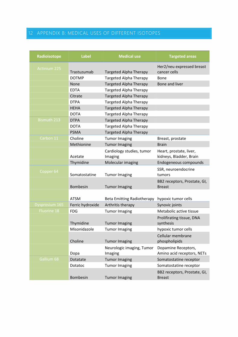
12 APPENDIX B: MEDICAL USES OF DIFFERENT ISOTOPES
Radioisotope Label Medical use Targeted areas
Actinium 225 Trastuzumab Targeted Alpha Therapy
Her2/neu expressed breast cancer cells
DOTMP Targeted Alpha Therapy Bone None Targeted Alpha Therapy Bone and liver EDTA Targeted Alpha Therapy Citrate Targeted Alpha Therapy DTPA Targeted Alpha Therapy HEHA Targeted Alpha Therapy DOTA Targeted Alpha Therapy
Bismuth 213 DTPA Targeted Alpha Therapy DOTA Targeted Alpha Therapy PSMA Targeted Alpha Therapy
Carbon 11 Choline Tumor Imaging Breast, prostate Methionine Tumor Imaging Brain
Acetate
Cardiology studies, tumor Imaging
Heart, prostate, liver, kidneys, Bladder, Brain
Thymidine Molecular imaging Endogeneous compounds
Copper 64 Somatostatine Tumor Imaging
SSR, neuroendocrine tumors
Bombesin Tumor Imaging
BB2 receptors, Prostate, GI, Breast
ATSM Beta Emitting Radiotherapy hypoxic tumor cells
Dysprosium 165 Ferric hydroxide Arthritis therapy Synovic joints Fluorine 18 FDG Tumor Imaging Metabolic active tissue
Thymidine Tumor Imaging
Prolifirating tissue, DNA synthesis
Misonidazole Tumor Imaging hypoxic tumor cells
Choline Tumor Imaging
Cellular membrane phospholipids
Dopa
Neurologic imaging, Tumor Imaging
Dopamine Receptors, Amino acid receptors, NETs
Gallium 68 Dotatate Tumor Imaging Somatostatine receptor Dotatoc Tumor Imaging Somatostatine receptor
Bombesin Tumor Imaging
BB2 receptors, Prostate, GI, Breast
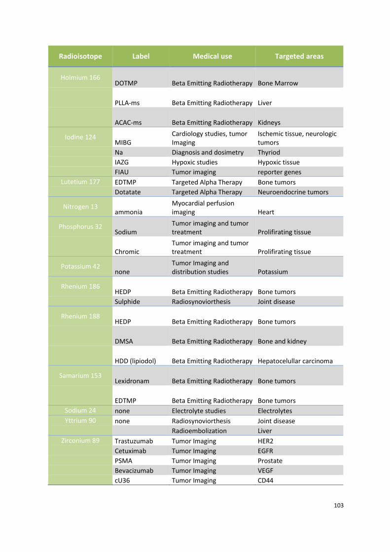
103
Radioisotope Label Medical use Targeted areas
Holmium 166 DOTMP Beta Emitting Radiotherapy Bone Marrow
PLLA-ms Beta Emitting Radiotherapy Liver
ACAC-ms Beta Emitting Radiotherapy Kidneys
Iodine 124 MIBG
Cardiology studies, tumor Imaging
Ischemic tissue, neurologic tumors
Na Diagnosis and dosimetry Thyriod IAZG Hypoxic studies Hypoxic tissue FIAU Tumor imaging reporter genes
Lutetium 177 EDTMP Targeted Alpha Therapy Bone tumors Dotatate Targeted Alpha Therapy Neuroendocrine tumors
Nitrogen 13 ammonia
Myocardial perfusion imaging Heart
Phosphorus 32 Sodium
Tumor imaging and tumor treatment Prolifirating tissue
Chromic
Tumor imaging and tumor treatment Prolifirating tissue
Potassium 42 none
Tumor Imaging and distribution studies Potassium
Rhenium 186 HEDP Beta Emitting Radiotherapy Bone tumors
Sulphide Radiosynoviorthesis Joint disease
Rhenium 188 HEDP Beta Emitting Radiotherapy Bone tumors
DMSA Beta Emitting Radiotherapy Bone and kidney
HDD (lipiodol) Beta Emitting Radiotherapy Hepatocelullar carcinoma
Samarium 153 Lexidronam Beta Emitting Radiotherapy Bone tumors
EDTMP Beta Emitting Radiotherapy Bone tumors
Sodium 24 none Electrolyte studies Electrolytes Yttrium 90 none Radiosynoviorthesis Joint disease
Radioembolization Liver Zirconium 89 Trastuzumab Tumor Imaging HER2
Cetuximab Tumor Imaging EGFR PSMA Tumor Imaging Prostate Bevacizumab Tumor Imaging VEGF cU36 Tumor Imaging CD44
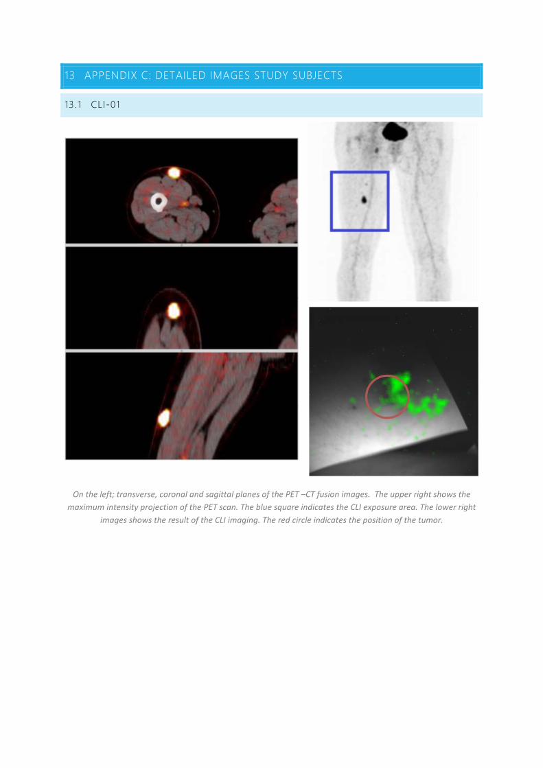
13 APPENDIX C: DETAILED IMAGES STUDY SUBJECTS
13.1 CLI-01
On the left; transverse, coronal and sagittal planes of the PET –CT fusion images. The upper right shows the maximum intensity projection of the PET scan. The blue square indicates the CLI exposure area. The lower right
images shows the result of the CLI imaging. The red circle indicates the position of the tumor.
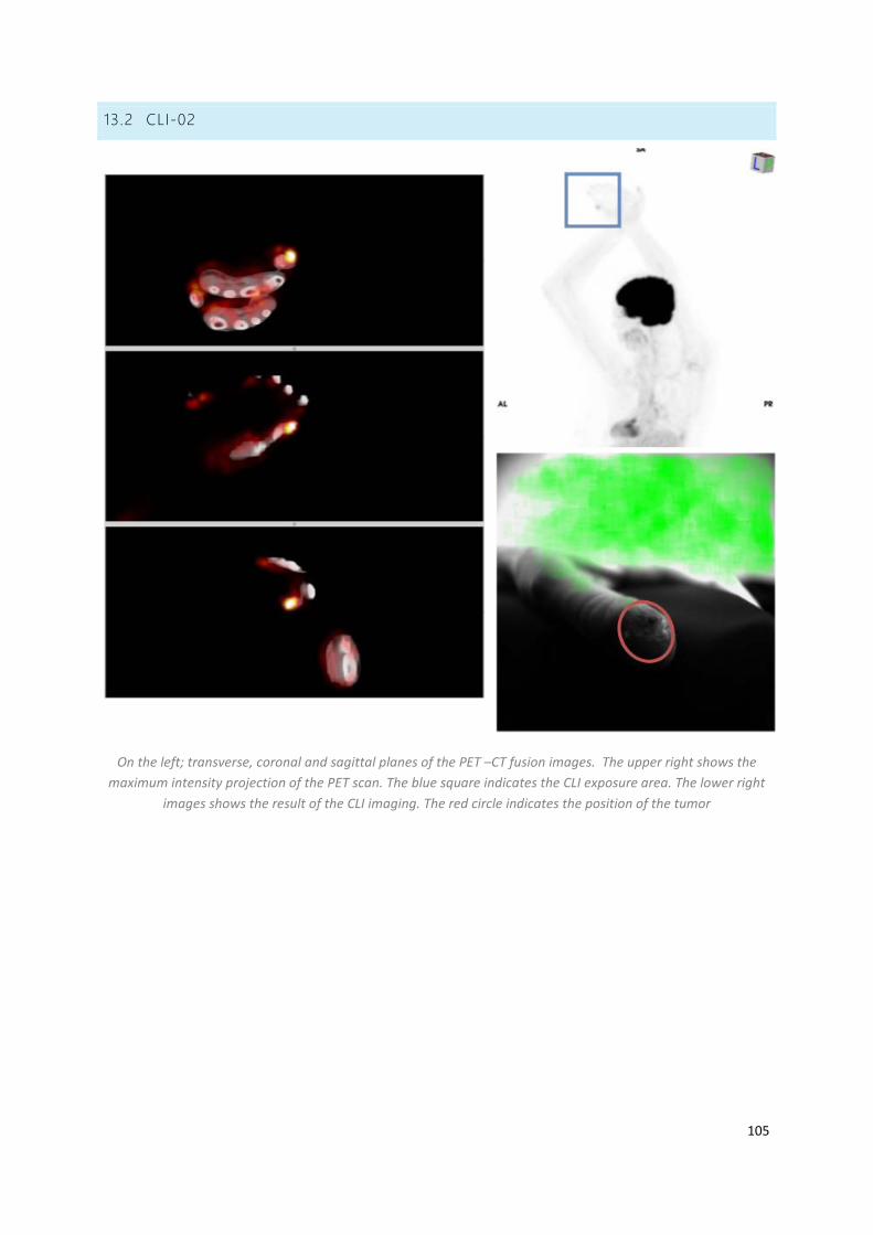
105
13.2 CLI-02
On the left; transverse, coronal and sagittal planes of the PET –CT fusion images. The upper right shows the maximum intensity projection of the PET scan. The blue square indicates the CLI exposure area. The lower right
images shows the result of the CLI imaging. The red circle indicates the position of the tumor

13.3 CLI-03
On the left; transverse, coronal and sagittal planes of the PET –CT fusion images. The upper right shows the maximum intensity projection of the PET scan. The blue square indicates the CLI exposure area. The lower right
images shows the result of the CLI imaging. The red circle indicates the position of the tumo
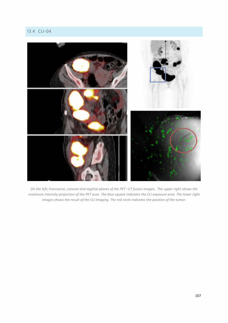
107
13.4 CLI-04
On the left; transverse, coronal and sagittal planes of the PET –CT fusion images. The upper right shows the maximum intensity projection of the PET scan. The blue square indicates the CLI exposure area. The lower right
images shows the result of the CLI imaging. The red circle indicates the position of the tumor.
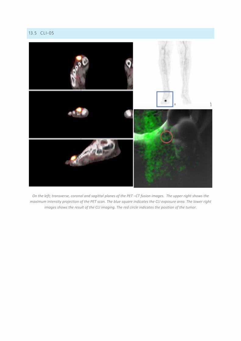
13.5 CLI-05
On the left; transverse, coronal and sagittal planes of the PET –CT fusion images. The upper right shows the maximum intensity projection of the PET scan. The blue square indicates the CLI exposure area. The lower right
images shows the result of the CLI imaging. The red circle indicates the position of the tumor.

109
14 APPENDIX D: METC APPROVAL