determining the ideal ratio of worker and machine …
TRANSCRIPT

1
DETERMINING THE IDEAL RATIO OF WORKER AND MACHINE TO INCREASE OPERATOR’S
UTILIZATION
By Ayu Pangestuti Chasanah Putri
ID No. 004200900010
A Thesis presented to the Faculty of Engineering President University in partial fulfillment of the requirements of Bachelor Degree in
Engineering Major in Industrial Engineering
2013

i
THESIS ADVISOR
RECOMMENDATION LETTER
This thesis entitled “Determining the Ideal Ratio of Worker and
Machine to Increase Operator’s Utilization” prepared and
submitted by Ayu Pangestuti Chasanah Putri in partial fulfillment
of the requirements for the degree of Bachelor of Engineering in the
Faculty of Engineering has been reviewed and found to have satisfied
the requirements for a thesis fit to be examined. I therefore
recommend this thesis for Oral Defense.
Cikarang, Indonesia, January 2013
Johan Oscar Ong, ST.,MT.

ii
DECLARATION OF ORIGINALITY
I declare that this thesis, entitled “Determining the Ideal Ratio of
Worker and Machine to Increase Operator’s Utilization” is to the
best of my knowledge and belief, an original piece of work that has
not been submitted, either in whole or in part, to another university to
obtain a degree.
Cikarang, Indonesia, January 2013
Ayu Pangestuti Chasanah Putri

iii
AUTHOR STATEMENT I, the undersigned bellow,
Name : Ayu Pangestuti Chasanah Putri ID Number : 004200900010 Faculty/ Study Program : Industrial Engineering
state that,
1. Considering a development of science, I hereby assign, transfer, and convey all rights, title, and its accompanying original tables and figures, including copyright ownership of this thesis entitled “Determining the Ideal Ratio of Worker and Machine to Increase Operator’s Utilization” to the President University in the event that this thesis is published by President University.
2. In making this assignment of ownership, I understand that all accepted thesis become the permanent property of President University and may not be published elsewhere without written permission from President University.
3. President University reserves the right to store, transfer media/ transfer format, manage in softcopy for academic purposes without needing to ask permission from me as long as my name is still listed as the author.
4. I am willing to underwrite and insure privately, without involving the President University any lawsuits arising from the infringement of copyright in this thesis.
This statement is truly made to be utilized as deemed. Cikarang, January 2013 Ayu Pangestuti C.P.

iv
DETERMINING THE IDEAL RATIO OF WORKER
AND MACHINE TO INCREASE OPERATOR’S
UTILIZATION
By
Ayu Pangestuti Chasanah Putri
ID No. 004200900010
Approved by,
Johan Oscar Ong, ST.,MT. HerwanYusmira, B.Sc. MET,MTech.
Thesis Advisor Program Head of Industrial Engineering
Dr. –Ing Erwin Sitompul, M. Sc.
Dean of the Faculty of Engineering

v
ABSTRACT
This thesis is mainly focused on determining the ideal ratio of worker and
machine to increase operator’s utilization in auto rooting process area. Low
operator’s utilization could give impact to operator productivity and cost of
production. Therefore, the ideal ratio of worker and machine should be
determined to avoid excess resource. In order to determine the ratio of worker and
machine, a time study should be conducted. By using time study the standard time
of operator could be established, and it will be used to create a simulation model
of ideal worker and machine ratio. There are three scenarios of ideal worker and
machine ratio that the author made. Those three scenarios are compared by using
Bonferroni approach to get the best scenario of ideal worker and machine ratio.
The result of Bonferroni approach shows that the ideal ratio of worker and
machine is one operator for three machines. By implement this ideal ratio, the
operator utilization can be increased up to 26% and the operator productivity can
be increased up to 67%.
Keywords: worker and machine ratio, worker and machine utilization,
productivity, time study, simulation model, Bonferroni approach.

vi
ACKNOWLEDGEMENT Thanks to Allah for the blessings and power so the author can finish this research
as partial fulfillment of the requirements of Bachelor Degree in Industrial
Engineering. This research is hardly to be done without a big support from many
parties. Therefore, the author would like to deliver her gratitude to:
1. Beloved family, thank you for the never-ending support and everlasting love.
2. Mr. Johan Ocscar Ong, thank you for guidance and support in doing this
research.
3. All my lectures in President University, thank you for giving the knowledge
through my university years.
4. Mrs. Ngatmi and all leaders in Auto Rooting process area for the opportunity
to conduct research in their area and also for guidance, encouragement, and
support in completing this research.
5. Mrs. Diery I.R. Sembiring, Mr. Dahliar Dalfi and all LSC team for help,
advice and big support during the research.
6. Industrial Engineering students and all university students especially batch
2009, thanks for the friendship and togetherness in pursuing for the bachelor
degree.
7. Dirga Sapto Nugratama, thanks for the spirit, motivation, love, and pray.
8. Other parties that help the author and could not be mentioned one by one.

vii
TABLE OF CONTENTS
THESIS ADVISOR RECOMMENDATION LETTER……………………….. .…..i
DECLARATION OF ORIGINALITY………………………………………… .….ii
AUTHOR STATEMENT……………………………………………………… ….iii
APPROVAL PAGE……………………………………………………………. .…iv
ABSTRACT……………………………………………………………………. ….v
ACKNOWLEDGEMENT……………………………………………………… …vi
TABLE OF CONTENTS………………………………………………………. ...vii
LIST OF TABLES…………………………………………………………....... ....xii
LIST OF FIGURE……………………………………………………………… …xiv
LIST OF TERMINOLOGIES…………………………………………………. …xvi
CHAPTER I INTRODUCTION…………………….………………………..... ......1
1.1 Problem Background……………………………………………………. ......1
1.2 Problem Statement…………….………………………………………… ......3
1.3 Objective………………………….…………………………….……..… ......3
1.4 Scope………………………………….……………………………….… ......3
1.5 Assumption……………………………….……………………………… ......3
1.6 Research Outline…………………………….…………………………… ......4
CHAPTER II LITERATURE STUDY………………………………………… ......5
2.1 Recording and Analysis Tools…………………………………………… ......5
2.1.1 Worker and Machine Process Chart………………………………… ......5
2.1.2 Gang Process Chart………………………………………………… ......9
2.2 Quantitative Tools, Workers, and Machine Relationship………………. ......9

viii
2.2.1 Synchronous Servicing…………………………………………….. ......9
2.2.2Random Servicing…………………………………………………… ....10
2.3 Time Study……………………………………………………………… ....10
2.3.1 Cycle of Study……………………………………………………… ...12
2.3.2 Performance Rating………………………………………………… ...12
2.3.3 Allowance………………………………………………………….. ...14
2.3.4 Normality Test……………………………………………………… ....15
2.3.5 Uniformity Test……………………………………………………. ....15
2.3.6 Sufficiency Test……………………………………………………. ...16
2.4 Simulation………………………………………………......................... ....16
2.4.1 Model Verification and Validation………………………………… ....17
2.4.2 Number of Replication (Sample Size)……………………………… ....18
2.4.3Comparing Two Alternative System…………………………….…. ....20
2.4.4 Comparing More Than Two Alternative System………………….. ...21
2.5 Goal Programming……………………………………………………… ....22
2.5.1 The Weights Method………………………………………………. ....24
2.5.2 The Preemptive Method…………………………………………… ....25
CHAPTER III RESEARCH METHODOLOGY……………….……………… ...26
3.1 Initial Observation…………………………………………………......... ....27
3.2 Problem Identification…………………………………………………… ....27
3.3 Literature Study…………………………………………………………. ...27
3.4 Data Collection and Calculation………………………………………… ...28
3.5 Analysis and Development……………………………………………… ...28
3.6 Conclusion and Recommendation……………………………………… ...28
3.7 Detail Framework ……………………………………………………… ...29

ix
CHAPTER IV DATA COLLECTION AND ANALYSIS …………………… ...30
4.1 Current Condition in Auto Rooting Process Area……………………… ...30
4.1.1 Worker and Machine Utilization…………………………………… ….31
4.1.2 Operator Productivity……………………………………………… ….32
4.1.3 Labor Cost ………………………………………………………… ….33
4.2 Operator Standard Time ………………………………………………… …..34
4.2.1 Normality Test……………………………………………………… …..34
4.2.2 Uniformity Test……………………………………………………. ...35
4.2.3 Sufficiency Test……………………………………………………. ...36
4.2.4 Performance Rating……………………………………….………… ...36
4.2.5 Allowance………………………………………………………….. ...37
4.2.6 Standard Time……………………………………………………… ...37
4.3 Analysis and Development…………………………………………....... ...38
4.3.1 Number of Machine to be Assigned for One Operator…….……… …..38
4.3.2 Simulation Model – Current Condition………………………......... ....39
4.3.2.1 Location……………………………………………………… ....39
4.3.2.2 Entities………………………………………………………. ...40
4.3.2.3 Arrival ……………………………………………………… ...40
4.3.2.4 Resources…………………………………………………… ...40
4.3.2.5 Path Network………………………………………………… ….41
4.3.2.6 Variables…………………………………………………….. ….42
4.3.2.7 Processing…………………………………………………… ….42
4.3.2.8 Result of Simulation Model………………………………… ….42
4.3.2.9 Verification and Validation…………………………………. ...43
4.3.2.10 Number of Replication (Sample Size)……………………… ….46

x
4.3.2.11 Mathematical Model………………………………………. …47
4.3.3 Simulation Model – Scenario 1 : One Operator Handles Three
Machines…………………………………………………………............ ...49
4.3.4 Simulation Model – Scenario 2 : One Operator Handle Four
Machines…………………………………………………........................
...50
4.3.5 Simulation Model – Scenario 3 : Two Operators Handle
Seven Machines…………………………………………………………..
...51
4.4 Comparing Alternative System………………………………………..… ....52
4.4.1 Average Output per Machine……………………………………… ….53
4.4.2 Average Machine Utilization ……………………………………… ….57
4.4.3 Average Operator Utilization……………………………………… ….59
4.4.4 Comparison Result of Three Strategies……………………………. ...61
4.5 Proposed System: One Operator Handle Three Machines ……………… ….62
4.6 Comparison between Current System and Proposed System …………… ….65
CHAPTER V CONCLUSION AND RECOMMENDATION ………………… ...67
5.1 Conclusion……………………………………………………………… ...67
5.2 Recommendation……………………………………………………….. ...67
REFFERENCES……………………………………………………………..… ...69
APPENDICES………………………………..……………………………..… ...71
Appendix 1 Current worker and machine utilization …………………..… ...72
Appendix 2 Time Study………………………………………………..….. ...80
Appendix 3 Normality & Uniformity Test…………………………..……. ...82
Appendix 4 Sufficiency Test……………………………………………..… ....86
Appendix 5 Simulation Model – Current Condition……………………… ....88
Appendix 6 Simulation Model– Scenario 1: One Operator Handles Three
Machines…………………………………………………………...............
.101

xi
Appendix 7 Simulation Model - Scenario 2: One Operator Handles Four
Machines……………………………………………………………………
.104
Appendix 8Simulation Model - Scenario 3: Two Operators Handle Seven
Machines………….……………………………………….......................... .107
Appendix 9 Critical Value for Student’s t Distribution…………………... .112
Appendix 10 Proposes System……………………………………………. .113

xii
LIST OF TABLE
Table 2.1Time study form……………………………………………………… .11
Table 2.2 Recommended number of observation cycle………………………… .13
Table 4.1 Worker utilization………………………………………………….... .31
Table 4.2 Machine utilization………………………………………………...... .31
Table 4.3 Current worker and machine utilization…………………………...... .32
Table 4.4 Average output per day per operator………………………………… .33
Table 4.5 Result of time study current auto rooting process…………………… .34
Table 4.6 Result of normality test…………………………………………….... .35
Table 4.7 Result of sufficiency test …………………………………………… .36
Table 4.8 Result of time study current auto rooting process …………………… .38
Table 4.9 Result of two machine for one operator…………………………….. .43
Table 4.10 Result of 16 replications………………………………………….... .46
Table 4.11 Result of scenario 1: three machines for one operator……………… .50
Table 4.12 Result of scenario 2: four machines for one operator……………… .51
Table 4.13 Result of scenario 3: seven machines for two operators…………… .53
Table 4.14 Result of Bonferroni approach for average output per machine…… .55
Table 4.15 Result of Bonferroni approach for average machine utilization…… .57
Table 4.16 Result of Bonferroni approach for average machine utilization…… .59
Table 4.17 Comparison of three strategies……………………………………… .61

xiii
Table 4.18 Score of three strategies…………………………………………..... .62
Table 4.19 Result one operator handle three machines ………………………… .62
Table 4.20 One operator handle three machine………………………………… .63
Table 4.21 Comparison between current and proposed system………………… .65

xiv
LIST OF FIGURE
Figure 2.1 Worker and machine process chart for milling machine operation.... …6
Figure 2.2 Another type of worker and machine process chart………………... …7
Figure 2.3 Gang process chart for operation of hydraulic extrusion process..… …8
Figure 3.1 Research methodology……………………………………………… ..26
Figure 3.2 Detail framework of the research…………………………………… .29
Figure 4.1 Auto rooting process chart…………………………………………. .30
Figure 4.2Auto rooting process layout………………………………………… .30
Figure 4.3 The location in simulation………………………………………….. .39
Figure 4.4 Display of the location in simulation………………………………. .39
Figure 4.5 The entities in simulation …………………………………………… .40
Figure 4.6 The arrival in simulation…………………………………………… .40
Figure 4.7 The resources in simulation……………………………………….… .41
Figure 4.8 The path in simulation……………………………………………… .41
Figure 4.9 Display of path network in simulation……………………………… .41
Figure 4.10 Variables in simulation……………………………………………. .42
Figure 4.11 Processing in simulation…………………………………………… .42
Figure 4.12 Display of running simulation……………………………………… .43
Figure 4.13 Display of trace result……………………………………………… .44
Figure 4.14 Display of debugger result………………………………………… .44

xv
Figure 4.15 Result of simulation modeling……………………………………. .45
Figure 4.16 Display of simulation modeling, three machines for one operator ………………………………………………………………….………
49
Figure 4.17 Display of simulation modeling, four machines for one operator…………………………………………………………………………
.50
Figure 4.18 Display of simulation modeling, seven machines for two operators…………………………………………………………………………
.52

xvi
LIST OF TERMINOLOGIES
Allowance : Time added to normal time to provide for personal
delays, unavoidable delays, and fatigue.
Auto rooting : Rooting process that use semi-automatic machine.
Confidence interval : A range within which the researches can have a
certain level of confidence that the true mean falls.
Cycle time : The period required to complete one cycle of
operation or to complete a function, job, or task
from start to finish.
Efficiency : The comparison of what is actually produced with
what can be achieved with the some consumption
of resources.
Hair yarn : The yarn that will be used as doll’s hair.
Inspection : The process of checking the product’s quality after
finishing a kind of production process.
Johnson wax : A liquid that used in rooting process to make hair
yarn easily attach to doll’s scalp.
Normal time : The amount of time required for a repeated
operation by an experienced worker of average
skill working at a normal pace.
Painted head : The output of painting process that will be used as

xvii
an input for rooting process or the doll’s head
without hair.
Performance rating : A process to evaluate the performance of operator.
Productivity of operator : Amount of product that can be produced by one
operator in one hour.
PT. X : A manufacturing company that produce dolls.
Rooted head : Output of rooting process or doll’s head with hair.
Rooting : The process of stitching hair yarn into the doll’s
scalp.
Significance level : The probability that the test will reject null
hypothesis when the hypothesis is true.
Standard time : The time for completing the work process with
allowance.
Time study : The examination and analysis of time and motion
required to complete an action.

1
CHAPTER I
INTRODUCTION
1.1 Problem Background
Nowadays, global competition in the world of industry has been risen up. Every
company is competes against each other to win customer hearts. One of the ways
is by reducing their cost while maintain their quality or if it possible improve their
quality. In order to reduce cost of production, a company should eliminate the
excess cost waste in the system. Another way is by increasing the efficiency.
Having high efficiency is important for the company. By having high efficiency, a
company could get many benefits. A company will be able to produce more
output with fewer resources. This could be happen because all resources such as
man, materials, machines, and space are well-utilized. Thus, the excess resources
could be allocated to other project.
Having high efficiency is also important for PT.X. PT.X is a part of a
multinational company that produces many kind of toy. One of the toys is called
fashion doll. Fashion dolls are produced in two Subsidiaries Company, ABC in
China and PT.X in Indonesia. Headquarter can choose which company they will
give the order. The one who can give better quality and better price will get more
order from headquarter. That is why PT.X always make continues improvement in
all manufacturing process area to produce better quality with lower cost of
production.
In PT.X, the process of making doll can be classified into three major processes
which are costume process, body process, and head process. Costume process
starting with costume development and then continues with costume sewing
production. Another process is body process that consists of two major processes
which are injection molding and torso assembly. Injection molding is the process
of making part of doll’s body and then the part will be assembled in torso
assembly process. The last is head process. Head process started with rotocast

2
process to produce basic head and then the basic head will go to face decoration
process. After face decoration process is complete, the head will go to rooting
process to get doll’s hair.
Rooting is a part of head process that stitching the hair yarn into the doll’s scalp to
make the hair attached onto its scalp area. In PT.X, rooting process can be
classified into two processes, which are manual rooting process and auto rooting
process. Manual rooting uses manual machine to assist the process. Operator
stitch hair yarn to the scalp manually one by one. In addition, auto rooting use
semi-automatic machine that can stitch hair yarn automatically to the scalp.
Operator just needs to load or unload head to the machine and the machine will
run automatically. That machine can reduce the number of operator because one
operator can handle more than one machine. With that machine, the number of
output can also increase because the speed of that machine is higher than
operator’s speed in manual machine. In short, we can say that auto rooting is more
beneficial than manual rooting.
Although auto rooting process is better than manual rooting process, the company
should not be satisfied. Auto rooting process still has several problems; such as
low operator utilization. The initial observation shows that the operator in auto
rooting process area still has 45% idle time. This situation results to some
consequences such as low productivity and high cost of production. This
condition can be improved by check whether all resources is properly used or not.
One of resources that should be checked is a man power. The author believes that
operator utilization can be increase by increasing man machine ratio due to high
idle time of operator. In auto rooting process, currently man machine ratio is 1:2.
It means one operator handle two machines. If one operator can handle more than
two machines, not only operator utilization that will be increase but also the
productivity of operator will be increase too. Moreover, the cost of production
will decrease because the company can reduce the labor cost. Therefore some
study need to be held to see this opportunity.

3
1.2 Problem Statement The background of the problem leads into the statement below.
• How to determine the ideal ratio of worker and machine to increase
operator’s utilization and reduce labor cost in auto rooting process area?
1.3 Objectives
The main objective of this research is finding the way to determine the ideal ratio
of worker and machine to increase operator’s utilization and reduce labor cost in
auto rooting process area.
1.4 Scope
Due to limited time and resources in doing this research, there will be some scope
in the observation:
1. The observation focus on auto rooting process.
2. The observation is done in September 28th – October 13th 2012.
3. The observation of this research conducted only in shift 2.
1.5 Assumption
The author has assumption as follows:
1. The type of doll’s head observation is assumed to be the same which
means neglecting the variance of doll’s size and shape.
2. The material type of the doll’s head and hair yarn is assumed to be the
same.
3. The Auto Rooting machine performance is assumed to be the same and no
machine breakdown during the process.
4. The skill operator is the same because skill is not as variable in this
research.
5. There will be no defect in the midst of auto rooting process.

4
1.6 Research Outline
Chapter I Introduction
This chapter consists of the background of research, problem
statement, objectives, scope, and assumption of the study.
Chapter II Literature Study
In this chapter, all related concepts and theories are given. These
concepts and theories are expected to be useful for the reader when
reading the rest parts of this final project.
Chapter III Research Methodology
The flow of this research is explained in this chapter.
Chapter IV Data Collection and Analysis
The data observation is processed and analyze in this chapter.
Chapter V Conclusion and Recommendation
This chapter will give the conclusion result of this research, and
also recommendation for future research.
In this chapter, the problem and objectives of this research have been clearly
explained. Furthermore, the scope and assumption have also stated. These are
becoming the direction of this research. After having the direction, it is needed to
know the way to solve the problem in order to achieve the objectives. Therefore,
some previous studies about related subject are delivered in the next chapter.

5
CHAPTER II
LITERATURE STUDY
1.1 Recording and Analysis Tools
1.1.1 Worker and Machine Process Charts
According to Niebel and Freivalds (2003), the worker and process chart is used to
study, analyze and improve on the workstation at a time. The exact time
relationship between the working cycle of the person and the operating cycle of
the machine is showed by this chart. It is important to get a fuller utilization of
both worker and machine time, and a better balance of the work cycle. The areas
in which both idle machine time and worker time occur is clearly showed in the
complete worker and machine process chart. These areas are a good place to start
in effecting improvement.
Figure 2.1 shows worker and machine process chart for milling machine operation.
On that figure, the right side shows the working time and the idle time of the
machine and the left side shows the operations and time for the worker. A solid
line drawn vertically shows the employee’s working time and a break in the
vertical work-time line signifies idle time. Similarly, a solid vertical line under
each machine heading indicates machine operating time and break in the vertical
machine line designates idle machine time. A dotted line under the machine
column indicates loading and unloading machine time. During that time, the
machine is neither idle nor productive.
Another method of constructing worker and machine process chart for two
machines is shown in figure 2.2. Idle time is shown as dotted spaces, using the
symbol “O” for the operator and “M” for the machine. Machine interference is
shown as black space.

6
Figure 2.1 Worker and machine process chart for milling machine operation
Source: Methods, Standards, and Work Design Twelve Edition (Niebel and Freivalds, 2003)

7
Figure 2.2 Another type of worker and machine process chart
Source: Engineered Work Measurement (Karger and Bayha, 1977

8
0.07
0.08
0.04
0.06
0.45
0.10
0.15
Elevate Billet
Position Billet
Position Dummy0.05Build Pressure
Unlock DN
Locate and pushOut Shell
Withdraw Ram & Lock Die in Head
Extrude
MACHINE
OPERATION TIME
0.07
0.08
0.040.05
0.05
0.45
0.10
0.15
TIME
PRESS OPERATOR
OPERATION
Elevate Billet
Position Billet
Position Dummy
Build Pressure
Unlock DN
Locate and pushOut Shell
Extrude
0.12
0.11
0.04
0.05
0.68
Withdraw Ram & Lock Die in Head
TIMEOPERATIONOPERATION
ASSISTANT PRESS OPERATOR
Grease Die & Position Deck in Die Head
Idle Time
Run Head & Shell Out
Pull Die Off End of Rod
Shear Rod from Shell
TIMEOPERATION
FURNACE MAN
0.20
0.51
0.19
0.10
RearrangeBilliets in Furnace
Idle Time
Open Furnace Door and Remove BilletRam Billet from Furnace & Close Furnace Door
TIMEOPERATION
DUMMY KNOCKER
0.10
0.12
0.18
0.12
0.43
0.05
Position Shell on Small Press
Press Dummy Out on Shell
Dispose of Shell
Dispose of Dummy and Lay Aside Tengs
Idle Time
Grab Tengs & Move to Position
TIMEOPERATION
ASSISTANT DUMMYKNOCKER
0.12
0.68
0.20
Move Away from Small Press and Lay Aside Tengs
Idle Time
Guide Shell from Shear to Small Press
TIMEOPERATION
PULL-OUT MAN
0.20
0.15
0.12
0.08
Pull Rod Toward Cooling Rack
Walk Back Toward Press
Grab Rod withTengs and Pull Out
0.45
Straighten Rod End with Mellet
Mold Rod whileDie Removed at Press
WORKING TIME 1.00 MIN. 1.00 MIN. 0.32 MIN. 0.49 MIN. 0.57 MIN. 0.32 MIN. 1.00 MIN.
IDLE TIME 0 " 0 " 0.68 " 0.51 " 0.43 " 0.68 " 0 "
GANG PROCESS CHART OF PRESENT METHOD
Figure 2.3 Gang process chart for operation of hydraulic extrusion process
Source: Methods, Standards, and Work Design Twelve Edition (Niebel and Freivalds, 2003)

9
2.1.2 Gang Process Chart
The gang process chart is an adaptation of the worker and machine chart (Niebel
and Freivalds, 2003). The exact relationship between the idle and operating cycle
of the machine and the idle and operating times per cycle of workers who service
that machine is clearly showed by this chart. This chart reveals the possibilities for
improvement by reducing both idle operator time and idle machine time. Figure
2.3 illustrates a gang process chart for a process in which a large number of idle
work-hours exist, up to 18.4 hours per 8 hours shift.
2.2 Quantitative Tools, Workers and Machine Relationship
Beside worker and machine process chart, mathematical model is also can be used
to know the number of facilities that can be assigned to an operator (Niebel and
Freivalds, 2003). This can often be computed in much less time. A worker and
machine relationship is usually one of these types:
1. Synchronous servicing.
2. Completely random servicing.
3. Combination of synchronous servicing and random servicing.
2.2.1 Synchronous Servicing
Assigning more than one machine to one operator seldom results in the ideal case
where both the worker and the machine are occupied during the whole cycle. Such
ideal cases are referred to as synchronous servicing. The number of machine to be
assigned can compute as:
𝑁 = 𝑙+𝑀𝑙
(2-1)
where: N = Number of machines the operator is assigned
l = Total operator loading and unloading (servicing) time per machine
m = Total machine running time (automatic power feed)

10
2.2.2 Random Servicing
Random servicing situations are those cases in which it is not known when a
facility needs to be serviced and how long servicing takes. Mean values are
usually known or can be determined. With these mean values, the laws of
probability can provide a useful tool in determining the number of machines to
assign a single operator.
The successive terms of binomial expansion give a useful approximation of the
probability of 0, 1, 2, 3, ...,n machine down (where n is relatively small).
Assuming that each machine is down at random times during the day and that
probability of downtime is p and the probability of running time is q = (1 - p).
Each term of the binomial expansion can be expressed as probability of M (out of
N) machines down:
𝑃(𝑀𝑜𝑓𝑁) = 𝑁!𝑀!(𝑁−𝑀)!
𝑝𝑀𝑞𝑁−𝑀 (2-2)
2.3 Time Study
Time study frequently defined as a method of determining a fair day’s work
(Niebel and Freivalds, 2003). Fair day’s work is the amount of work that can be
produced by a qualified employee when working at a normal pace and effectively
utilizing his time where work is not restricted by process limitations. In time study,
the operation should be divided into groups of motions known as elements.
Elements should be broken down into divisions that are as fine as possible but not
too small that reading accuracy is sacrificed. Table 2.1 shows a time study form.
On this form, analyst would record the various elements horizontally across the
top of the sheet, and the cycle studied would be entered vertically row by row.

11
Table 2.1 Time study form
Source: Methods, Standards, and Work Design Tenth Edition (Niebel and Freivalds,2003)
Column R is provided for ratings, column W for watch reading, column OT for
observed time, column NT for normal time. The value NT is getting from the
formula below.
NT = OT × R/100 (2-3)
R W OT NT R W OT NT R W OT NT R W OT NT R W OT NT R W OT NT R W OT NT
Sym w1 w2 OTABCDEFG
Elapsed Time Variable FatigueTEBS SpecialTEAF Total Allowance %Total Check Time Remarks:
Synthetic Time % Unaccounted TimeObserved Time Recording Error %
Effective TimeIneffective Time
Rating Check Total Recorded Time
Description Finishing Time Personal NeedsStarting Time Basic Fatigue
Total Standard Time (sum standard time for all elements)Foreign Elements Time Check Allowance Summary
Standard TimeNo. OccurrencesElemental Std. Time% AllowanceAverage NTNo. ObservationsTotal NTAverage OT
20Summary
Total OT
171819
141516
111213
89
10
567
234
Notes Cycle1
Element No. and Description
1 2 3 4
Time study Observation Form Study No.: Date:Operation: Operator: Oberver:
6 75

12
Time elapsed before study (TEBS) is the readout when the analyst snaps the
watch at the start of the first element. Time elapsed after study (TEAS) is the last
readout when the analyst snaps the watch at the very end of the study. These
quantities are totaled forming check time. Effective time is got from the summary
of all observed times. Ineffective time is got from the summary of all foreign
elements time. The summary of checkout time, effective time and ineffective time
become total recorded time. The difference between the starting time and
finishing time equals to elapsed time. The difference between the total recorded
time and elapsed time is called unaccounted time. In a good study, this value
would be zero. The unaccounted time divided by the elapsed time is a percentage
of reading error. If the reading error exceeds 2%, the time study should be
repeated.
2.3.1 Cycle of Study
According to Barnes (1980), a preliminary observation should be taken before
conducting time study. In preliminary observation, small number of sample cycle
time is taken (usually 5 samples). This preliminary cycle time will be used for
determining the number of sample for real time study. The general electric
company has established a recommended number of observation cycle based on
length of the process. The recommendation for the number of observation cycle is
presented in the table 2.2.
2.3.2 Performance Rating
Performance rating is probably the most important step in the entire work
measurement procedure. It is based on the experience, training, and judgment of
the work measurement analysis. The rating factor is based on the speed or tempo
of the output or on the performance of the operator compared to that of a qualified
worker. Experience and judgment are still the criteria for determining the rating
factor (Niebel and Freivalds, 2003).

13
Table 2.2 Recommended Number of Observation Cycle
Source: Niebel’s Methods, Standards, and Work Design Twelve Edition (Niebel and Freivalds, 2003)
The basic principle of performance rating is to adjust the average observed time
(OT) for each element performed during the study to the normal time (NT) that
would be required by the normal operator to perform the same work:
NT = OT x R/100 (2-4)
R is expressed as a percentage, with 100 percent being standard performance by a
normal operator. To do a fair job of rating, the time study analyst must be able to
disregard personalities and other varying factors, and consider only the amount of
work being done per unit of time, as compared to the amount of work that the
normal operator would produce.
Performance rating system consists of four methods. Those four methods are
speed rating, the Westinghouse system, synthetic rating, and objective rating.
Westinghouse system is one of commonly used for rating system (Niebel and
Freivalds, 2003).
Cycle Time (minutes) Recommended number of cycles 0.1 200
0.25 100 0.5 60
0.75 40 1 30 2 20
2.00-5.00 15 5.00-10.00 10
10.00-20.00 8 20.00-40.00 5
>40.00 3

14
2.3.3 Allowance
The time added to normal time to provide for personal delays, unavoidable delays,
and fatigue is called allowance. Allowance are applied to three parts of the study
which are total cycle time, machine time only, and manual effort time only.
Allowance is given because no operator can maintain an average pace every
minute of the working day. There are 2 allowances that usually use in time study.
First is constant allowance and the second is special allowance. Constant
allowances consist of personal need and basic fatigue. Personal need allowance
includes cessations in the work necessary for maintaining the general well-being
of the employees. For example, trips to the restroom or drinking. The general
working conditions and class of work influence the time necessary for personal
delays. There is no scientific basis for this allowance, however, detailed
production records that mostly 5% allowance for personal time (Niebel and
Freivalds, 2003).
Basic fatigue allowance is a constant to account for the energy expand to carry out
the work and to alleviate monotony. A value 4% of normal time is considerate
adequate for an operator who is doing a light work, while seated, under good
working conditions, with no special demands on the sensory or motor systems
(ILO, 1957).There are many variable fatigue allowances that have no exact value
of allowance, including abnormal posture, use of force or muscular energy (lifting,
pulling or pushing), bad light, atmospheric conditions (heat and humidity), noise
level, tediousness, etc.
An allowance must be added to the normal time to arrive at a fair standard time
that can reasonably be achieved by the operator since the time study is taken over
a relatively short period and since foreign elements should have been removed in
determining the normal time. Standard time (ST) is the time required for a fully
qualified, trained operator, working at standard pace and exerting average effort to
perform the operation.
S𝑇 = 𝑁𝑇 + (𝑁𝑇 𝑥 𝑎𝑙𝑙𝑜𝑤𝑎𝑛𝑐𝑒%) = 𝑁𝑇 𝑥 (1 + 𝑎𝑙𝑙𝑜𝑤𝑎𝑛𝑐𝑒%) (2-5)

15
2.3.4 Normality Test
Normality test is used to determine whether the data observed normally
distributed or not. To test formally for normality, Anderson-Darling test is used
with the help of Minitab 14 software. The test uses significant level (α) and the
total number of data (n) to test the data is normally distributed or not. Then
compare the result of p-value with the significance level. The statistical
hypotheses consist of two hypotheses:
H0: The data is normally distributed.
H1: The data is not normally distributed.
After the significant level (α) is chosen, the decision is made. If P is less than or
equal to α, reject H0 and if P is greater than α, fail to reject H0. It means null
hypotheses is accepted and normally distributed. Thus, the data are applicable for
the next analysis.
2.3.5 Uniformity Test
After normality test, the uniformity test is conducted. The purpose of uniformity
test is to make sure that all data in the expected range area. If the data outside the
limit thus, that data must be removed. The steps of conducting uniformity test are
as follows (Sutalaksana et al, 2006):
Calculate average observed time (�̅�) for each operation
�̄� = ∑ 𝑥𝑖𝑁𝑖=1𝑁
(2-6) Calculate the standard deviation (σ) of each operation
σ = �∑ (𝑥𝑖− 𝑥 ̄)2𝑁𝑖=1𝑁−1
(2-7) Determine the Upper Control Limit (UCL) and Lower Control Limit
(LCL). 𝑈𝐶𝐿 = �̅� + 3𝜎𝑥 (2-8)
𝐿𝐶𝐿 = �̅� − 3𝜎𝑥 (2-9)

16
2.3.6 Sufficiently Test
Sufficiency is conducted to know the data observed is sufficient or not for
determined confidence level. The following formula is to calculate how many
observations must be done to reach 5% significance level and 95% confidence
level (Sutalaksana et al, 2006). The formula can be expressed as follows:
𝑁′ = �40 �𝑁.∑𝑥𝑖
2−(∑𝑥𝑖)2
∑𝑥𝑖�
2
(2-10)
N’ is the number of observation needed and N is number of preliminary data. If
N >N’ so the preliminary data is enough but if N < N’ thus, it is needed to take
more data until the number of observation.
2.4 Simulation
Simulation is defined by Oxford American Dictionary (1980) as a way to
reproduce the condition of a situation, as by means of a model, for study or testing
or training, etc. Simulation can be done in many ways; one of them is by a
computer program. According to Schriber (1987), simulation is the modeling of a
process or system in such a way that model mimics the response of the actual
system to events that take place over. Simulation is essentially an experimentation
tool in which a computer model of new or existing system is created for the
purpose of conducting an experiment. Simulation avoids the expensive, time-
consuming, and disruptive nature of traditional trial-and-error techniques (Harrel
et al, 2012).
The procedure for doing simulation follows the scientific method of formulating a
hypothesis, setting up experiment, testing the hypothesis through experimentation,
and drawing the conclusion about the validity of the hypothesis. For many
companies, simulation has become a standard practice when a new facility is
being planned or a process change is being evaluated. As a guideline, simulation
is appropriate if the following criteria hold true:
An operational (logical or quantitative) decision is being made.
The process being analyze is well defined and repetitive.

17
Activities and events are interdependent and variable.
The cost impact of the decision is greater than the cost of doing the
simulation.
The cost to experiment on the actual system is greater than the cost of
simulation.
Based on Harrel et al (2012), simulation has been using widely in recent days.
This happens because the simulation program is getting easier to be learned thus
the user will be very helped in developing a model. Moreover, simulation
accommodates many cases which are very useful to model a wide range of actual
events. Therefore, simulation has been used to help plan and make improvements
in many areas both manufacturing and service industries. One of the software to
do a simulation in those areas is ProModel.
ProModel is a simulation package designed specifically for ease of use, yet it
provides the flexibility to model any discrete event or continues flow process
(Harrel et al, 2012). Entities (the object being processed), locations (the place
where processing occur), resources (the agents used to process the entities), and
paths (the course of travel for entities and resources in moving between locations)
are the basic modeling objects in ProModel. Logical behavior such as the way
entities arrive and their routings can be defined with little programming using the
data entry table that are provided.
2.4.1 Model Verification and Validation
After the model has been built, model verification and validation should be done.
Model verification is the process of determining whether the simulation model
correctly reflects the conceptual model and model validation is the process of
determining whether the conceptual model correctly reflects the real system
(Harrel et al, 2012).Several techniques can be used to verify the model. Some of
the common ways include
• Conduct model code reviews.

18
• Check the output for reasonableness.
• Watch the animation for correct behavior.
• Using trace and debug facilities provided with the software.
In addition, there are also several techniques that can be used to validate the
model. Some of the techniques are the same as those used to verify the model.
These are the several techniques that described by Sargen (1998)
• Watching the animation.
• Comparing the actual system.
• Comparing with other models.
• Conducting degeneracy and extreme condition test.
• Checking for face validity.
• Testing against historical data.
• Performing sensitivity analysis.
• Running traces.
• Conducting Turing tests.
2.4.2 Number of Replication (Sample Size)
According to Harrel et al.(2012), the sample size or number of replication are used
to establish a particular confidence interval for a specified amount of absolute
error (denoted by e) between the point estimate of the mean 𝑥 �and the unknown
true mean µ. A point estimate is a single value estimate of a parameter of interest
(Harrel et al, 2012). Point estimate is calculated for mean and standard deviation
of the population. To estimate the mean of population (denoted as µ), the average
of the sample values (denoted as �̅�) is calculated by using the following equation.
�̄� = ∑ 𝑥𝑖𝑁𝑖=1𝑁
(2-11)
where n is the sample size (number of observation) and xi is the value of ith
observation.

19
The standard deviation for the population (denoted as σ) is similarly estimated by
calculating a standard deviation of the sample of values (denoted as s)
s = �∑ (𝑥𝑖− 𝑥 ̄)2𝑁𝑖=1𝑁−1
(2-12)
A point estimate gives little information about how accurately it estimates the true
value of the unknown parameter while interval estimates constructed using �̅� and
s that provides information about how far off the point estimate 𝑥 �might be from
the true mean µ. The method used to determine this is referred to as confidence
interval estimation (Harrel et al, 2012).
A confidence interval is a range within which we can have a certain level of
confidence that the true mean falls. The interval is symmetric about �̅� and the
distance that each endpoint is from �̅� is called half-width (hw). A confidence
interval is expressed as the probability P that the unknown true mean µ lies within
the interval �̅� ± hw. The probability P is called the confidence level (Harrel et al,
2012).
The following equation can be used to calculate the half-width of a confidence
interval for a given level of confidence.
ℎ𝑤 = �𝑡𝑛−1,𝛼/2�𝑠
√𝑛 (2-13)
where 𝑡𝑛−1,𝛼/2 is a factor that can be obtained from student’s table in appendix. α
is the complement of P. That is, α = 1 – P and is referred to the significance level.
Significance level is defined as the “risk level” or probability that µ will fall
outside the confidence level (Harrel et al, 2012).
After done with all the calculation above, the sample size (number of replication)
can be calculated by using the following equation.
𝑛′ = �(𝑍𝛼/2)𝑠𝑒
�2 (2-14)
Zα/2= t∞, α/2 and can be obtained from student’s table in appendix. The absolute
error (e) can be calculated by using equation below.

20
𝑒 = ℎ𝑤 (2-15)
𝑒 = �𝑡𝑛−1,𝛼/2�𝑠
√𝑛
2.4.3 Comparing Two Alternative System
Simulations are usually used to compare two or more alternative system to
identify the superior system relative to some performance measure. There are
several techniques to comparing alternative systems; one of them is Paired-t
confidence interval method. Paired-t confidence interval method is used to
compare two alternative systems. It requires that the observation from each
population be normally distributed and independent within a population. This
method also requires that the number of samples drawn from one population (n1)
equal to the number of samples drawn from the other population (n2).
In this method, we pair the observations from each population (x1j and x2j) to
define a new random variable x(1-2)j = x1j – x2j, for j = 1, 2, 3, …, n. The x1jdenoted
the jth observation from the first population sampled (the output from the jth
replication of the simulation model for the first alternative design), x2j denotes the
jth observation from the second population sampled (the output from the jth
replication of the simulation model for the second alternative design), and x(1-2)j
denotes the difference between the jth observations from the two populations. The
point estimators for new random variable are
𝑠𝑎𝑚𝑝𝑙𝑒 𝑚𝑒𝑎𝑛 = �̄�(1−2) = ∑ 𝑥(1−2)𝑗𝑁𝑖=1
𝑁 (2-16)
𝑠𝑎𝑚𝑝𝑙𝑒 𝑠𝑡𝑎𝑛𝑑𝑎𝑟𝑑 𝑑𝑒𝑣𝑖𝑎𝑡𝑖𝑜𝑛 = 𝑠(1−2) = �∑ �𝑥(1−2)𝑗−𝑥̄(1−2)�
2𝑁𝑖=1
𝑁−1 (2-17)
where�̄�(1−2) estimates µ(1−2) and 𝑠(1−2) estimates σ(1-2). The half-width equation
for the paired-t confidence interval is
ℎ𝑤 = �𝑡𝑛−1,𝛼/2�𝑠(1−2)
√𝑛 (2-18)

21
Thus, the paired-t confidence interval for an α level of confidence is
𝑃��̄�(1−2) − ℎ𝑤 ≤ µ(1−2) ≤ �̄�(1−2) + ℎ𝑤� = 1 − 𝛼 (2-19)
The hypotheses for an α level of confidence are
H0 = µ1 - µ2 = 0 or using the new “paired” notation µ(1-2) = 0
H0 = µ1 - µ2 ≠ 0 or using the new “paired” notation µ(1-2) ≠ 0
2.4.4 Comparing More Than Two Alternative System
If there are more than two alternative systems to be compared, Bonferroni
approach can be used. Given K alternative system design to compare, the null
hypothesis H0 and alternative H1 become
H0: µ1 = µ2 = µ3 = … = µk = µ for K alternative systems
H1 : µi≠µi’ for at least one pair i≠i’
where i and i’ are between K and i<i’. The null hypothesis H0 states that the
means from K populations are not different, and the alternative hypothesis H1
states that at least one pair of the means are different.
Bonferroni approach is similar to the two confidence interval method presented in
previous section. It is implemented by constructing a series of confidence
intervals to compare all system designs to each other. The number of pairwise
comparisons for K candidate design is calculated by using following equation.
𝑁𝑢𝑚𝑏𝑒𝑟 𝑜𝑓 𝑝𝑎𝑖𝑟𝑤𝑖𝑠𝑒 = 𝐾 (𝐾−1)2
(2-20)
A paired-t confidence interval is constructed for each pairwise comparison. For
example three candidate designs, denoted D1, D2, and D3, the three paired-t
confidence intervals are
𝑃 ��̄�(𝐷1−𝐷2) − ℎ𝑤 ≤ µ(𝐷1−𝐷2) ≤ �̄�(𝐷1−𝐷2) + ℎ𝑤� = 1 − 𝛼1

22
𝑃 ��̄�(𝐷1−𝐷3) − ℎ𝑤 ≤ µ(𝐷1−𝐷3) ≤ �̄�(𝐷1−𝐷3) + ℎ𝑤� = 1 − 𝛼2
𝑃 ��̄�(𝐷2−𝐷3) − ℎ𝑤 ≤ µ(𝐷2−𝐷3) ≤ �̄�(𝐷2−𝐷3) + ℎ𝑤� = 1 − 𝛼3
𝛼1= 𝛼2 = 𝛼3 = 𝛼 i is called individual significance level. Individual significance
level can be calculated by using equation below.
𝛼𝑖 = 𝛼𝐾(𝐾−1)/2
(2-21)
For i = 1, 2, 3, … ,K(K-1)/2
2.5 Goal Programming
According to Taha (2007), goal programming is a method to seek a compromise
solution based on the relative importance of each objective. Goal programming is
used where multiple (conflicting) objectives may be more appropriate. There are
two methods for solving goal programs. The two methods are the weight method
and the preemptive method. The weights method forms a single objective function
consisting of the weighted sum of the goals while preemptive method optimizes
the goals one at a time starting with the highest priority goal and terminating with
the lowest, never degrading the quality of a higher priority goal. The idea of goal
programming can be illustrated by the following example.
Example: Tax Planning1
Fairville is a small city with a population of about 20,000 residents. The city
council is in the process of developing an equitable city tax rate table. The annual
taxation base for real estate property is $550 million. The annual taxation base for
food and drugs and for general sales are $35 million and $55 million, respectively.
Annual local gasoline consumption is estimated at 7.5 million gallons. The city
council wants to develop the tax rates based on four main goals.
1. Tax revenues must be at least $16 million to meet the city’s financial
commitments.
2. Food and drug taxes cannot exceed 10% of all taxes collected.
1This example is based on Taha, 2007.
23
3. General sales taxes cannot exceed 20% of all taxes collected.
4. Gasoline taxes cannot exceed 2 cents per gallon.
Let the variables xp, xf, and xs represent the tax rates (expressed as proportions of
taxation bases) for property, food and drug, and general sales, and define the
variable xgas the gasoline tax in cents per gallon. The goals of the city council are
then expressed as
550xp + 35xf + 55xs + .075xg ≥ 16 (Tax revenue)
35 xf ≤ .1(550xp +35xf + 55xs + .075 xg) (Food/drug tax)
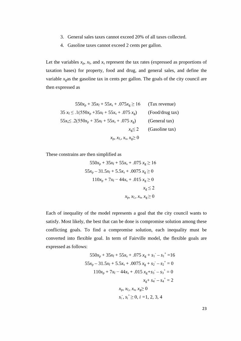
55xs≤ .2(550xp + 35xf + 55xs + .075 xg) (General tax)
xg≤ 2 (Gasoline tax)
xp, xf,, xs, xg≥ 0
These constrains are then simplified as
550xp + 35xf + 55xs + .075 xg ≥ 16
55xp – 31.5xf + 5.5xs + .0075 xg ≥ 0
110xp + 7xf − 44xs + .015 xg ≥ 0
xg ≤ 2
xp, xf,, xs, xg ≥ 0
Each of inequality of the model represents a goal that the city council wants to
satisfy. Most likely, the best that can be done is compromise solution among these
conflicting goals. To find a compromise solution, each inequality must be
converted into flexible goal. In term of Fairville model, the flexible goals are
expressed as follows:
550xp + 35xf + 55xs + .075 xg + s1- – s1
+ =16
55xp – 31.5xf + 5.5xs + .0075 xg + s2- – s2
+ = 0
110xp + 7xf − 44xs + .015 xg+s3- – s3
+ = 0
xg+ s4- – s4
+ = 2
xp, xf,, xs, xg≥ 0
si-, si
+ ≥ 0, i =1, 2, 3, 4

24
si- and si
+ are nonnegative variables that called deviational variables. They
represent the deviations below and above the right-hand side of constraints i.
The deviational variables si- and si
+ are by definition dependent, and hence cannot
be basic variables simultaneously. This means that in any simplex iteration, at
most one of the two deviational variables can assume a positive value. If the
original ith inequality is of the type ≤ and its si-> 0, then ith goal is satisfied.
Otherwise, if si+> 0, goal i is not satisfied. In essence, the definition of si
- and si+
allows meeting or violating the ith goal at will. This is the type of flexibility that
characterizes goal programming when it seeks a compromise solution. Naturally,
a good solution aims at minimizing the amount by which each goal is violated.
In Fairville model, given that the first three constrains are of the type ≥ and the
forth constrains is of the type ≤, the deviational variabless1-, s2
-, s3-, s4
- represent
the amounts by which the respective goals are violated. Thus, the compromise
solution tries to satisfy the following four objectives as much as possible:
Minimize G1 = s1-
Minimize G2 = s2-
Minimize G3 = s3-
Minimize G4 = s4+
2.5.1 The Weights Method
Suppose that the goal programming has n goals, the ith goal is given as
Minimize Gi, i = 1, 2, …, n
The combine objective function used in the weights method is defined as
Minimize z = w1G1 + w2G2 + … + wnGn
The parameters wi,i =1, 2, …, n, are positive weight that reflect the decision
maker’s preference regarding the relative importance of each goal (Taha, 2007).
For example, wi=1, for all i, signifies that all goals have equal weights. The
determination of the specific values of these weights is subjective.
25
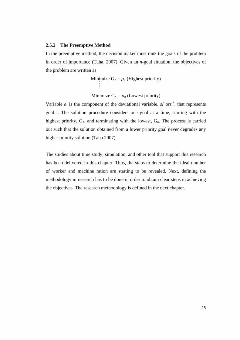
2.5.2 The Preemptive Method
In the preemptive method, the decision maker must rank the goals of the problem
in order of importance (Taha, 2007). Given an n-goal situation, the objectives of
the problem are written as
Minimize G1 = 𝜌1 (Highest priority)
Minimize Gn = 𝜌n (Lowest priority)
Variable 𝜌i is the component of the deviational variable, si- orsi
+, that represents
goal i. The solution procedure considers one goal at a time, starting with the
highest priority, G1, and terminating with the lowest, Gn. The process is carried
out such that the solution obtained from a lower priority goal never degrades any
higher priotity solution (Taha 2007).
The studies about time study, simulation, and other tool that support this research
has been delivered in this chapter. Thus, the steps to determine the ideal number
of worker and machine ration are starting to be revealed. Next, defining the
methodology in research has to be done in order to obtain clear steps in achieving
the objectives. The research methodology is defined in the next chapter.

26
CHAPTER III
RESEARCH METHODOLOGY
Research method of the project can be describe through following figure
Figure 3.1: Research methodology
Initial Observation
Problem Identification
Literature Study
Data Collection and Calculation
Analysis and Development
Conclusion and Recommendation
Initial Observation • Direct observation in PT X Indonesia
Problem Identification
• Analyze auto rooting process • Problem and objective identification • Determine scopes and assumption
Literature Study
• Recording and Analysis Tools • Quantitative Tools, Workers and
Machine Relationship • Time Study • Simulation
Data Collection and Calculation
• Observation by using time study Analysis and Development
• Time study • Analyze current condition • Create a model by using simulation • Propose a new system • Comparison current versus propose
system
Conclusion and Recommendation • Conclusion • Recommendation for the company and
future research

27
3.1 Initial Observation
The initial observation is done by observing auto rooting process area directly.
Auto rooting process was being observed because this area has several issues that
cannot be solved until now. Some limitations are given by PT. X to determine the
scope of the project.
3.2 Problem Identification
After observation in auto rooting process area is conducted, the author saw several
problems happened. One of the problems is the author saw that operators in auto
rooting process area still have idle time when they waited the process finish. The
author believed that some improvements could be conducted in this area. Then,
she shares this initial observation to her supervisor in PT. X and the supervisor
agrees that the author raise this problem as her project. Some scopes and
assumption are made to limit the project due the limitation of resources and time.
3.3 Literature Study
When the problem has been identified, literature should be conducted to find any
relevant references related to the problem. It is needed when doing problem
identification, data collection and tabulation, and data analysis. This activity will
provide the insight in terms of theories and concept as guidance for the author in
accomplishing the project. The gathered theories and concept are the ones
correlated with the problem identification and problem solving, which are worker
and machine process chart, gang process chart, time study, simulation, etc. Further
details of the theories and concepts used in this project can be found in Chapter II.

28
3.4 Data Collection and Calculation
Data will be collected based on time study analysis with several variables and
constraints. The data will be recorded on time-study form with video recorder.
Video recorder is used instead of stopwatch because by using a video recorder,
author can get more precise data based on evidence and the playback feature is
very useful to avoid the skipped activities. The author will break down the
elements and find the cycle time of every element. Normality and uniformity test
will keep the data from time study as the main tools valid. After get the cycle time,
the next step is to find the standard time and make the proposed system.
3.5 Analysis and Development
After having data collection and calculation, analyzing must be done. The author
will analyze the result of time study. The author will also analyze worker
utilization, machine utilization, and cost of production due to labor cost. After all
of the analysis done, author will propose new work arrangement for operator.
Since this final project has not been implemented, the new work arrangement
which resulted from the analysis is required to be developed into a model.
ProModel is a simulation program that will be used to develop that model. Then
the model has to be evaluated whether it gives improvement or not.
3.6 Conclusion and Recommendation
This is the last phase of this research. The author will conclude the improvements
and effects resulted from the solution implementation achieve the objectives or
not. In addition, the recommendation also includes in this phase. The
recommendation is addressed for both the readers and the company.

29
3.7 Detail Framework
The detail framework of this research is illustrated as follow.
Start
Initial Observation
Find abnormality?
Literature Study
Analyze current condition
Time study – record cycle time
Normality Test
Normal data?
Uniformity Test
Uniform data?
A
Worker and Machine Process Chart
Analysis and development
Propose improvement
Simulation
Significant result?
Compare current vs proposecondition
Conclusion and recommendation
End
Remove outliers data
Yes
No
Yes
No
Yes
No
Sufficiency Test
Sufficient data?
A
No
No
Yes
Get standard time
Yes
No
Figure 3.2 Detail framework of the research

30
CHAPTER IV
DATA COLLECTION AND ANALYSIS
4.1 Current Condition in Auto Rooting Process Area
Auto rooting machine is a great innovation that has successfully made by PT.X
three years ago. With auto rooting machine, the operator does not need to stitch
hair yarn to the doll’s scalp manually. The operator just need to load head to the
machine and the machine will run automatically. The detail process of auto
rooting shows at figure 4.1.Currently, there are 110 full auto rooting machines in
PT.X. Those machines run by 55 operators, with the composition two machines
for one operator. Figure 4.2 below show the layout of auto rooting machine.
Figure 4.2 Auto rooting process layout
Figure 4.1 Auto rooting process chart
Start
Load head to johnson wax
Unload head from johnson wax
Load head to machine
Unload head from machine
End
Inspection

31
4.1.1 Worker and Machine Utilization
In initial observation, the author saw that the idle time of the operator is high. It
can be seen directly if the author passes this area. This condition can be improved
by increasing worker utilization. To increase worker utilization, the author must
know the current condition of worker utilization. The author records operator’s
real jobs element by element include the movement from one machine to another
machine. Part of calculation can be seen at table 4.3 and the full calculation is
presented in appendix. The left column (Time) is the observed time and the right
column (Cumulative Time) is the cumulative of the observation time. Next to
Time column is the worker and machine detail job. The blue color shows the
running process, white color shows idle, and green color shows the movement of
operator from one machine to another machine. The following table shows the
result of worker and machine utilization.
Table 4.1 Worker utilization
WORKER Running Time Idle Time % Idle Time % Utilization Observation 1 283 s 115 s 41% 59% Observation 2 937 s 314 s 34% 66% Observation 3 1205 s 375 s 31% 69%
TOTAL 2425 s 804 s 35% 65%
Table 4.2 Machine utilization
MACHINE 1 Running Time Idle Time % Idle Time % Utilization Observation 1 283 s 30 s 11% 89% Observation 2 937 s 82 s 9% 91% Observation 3 1205 s 121 s 10% 90%
TOTAL 2425 s 233 s 10% 90% MACHINE 2 Running Time Idle Time % Idle Time % Utilization Observation 1 283 s 19 s 7% 93% Observation 2 937 s 98 s 10% 90% Observation 3 1205 s 130 s 11% 89%
TOTAL 2425 s 247 s 9% 91%

32
Table 4.3 Current worker and machine utilization
From the result above, it can be seen that the machine utilization is already good
which is above 90% utilization but the worker utilization still low which is 65%.
4.1.2 Operator Productivity
PTX use this calculation below to calculate operator productivity
𝑃𝑟𝑜𝑑𝑢𝑐𝑡𝑖𝑣𝑖𝑡𝑦 = 𝑇𝑜𝑡𝑎𝑙 𝑜𝑢𝑡𝑝𝑢𝑡𝑇𝑜𝑡𝑎𝑙 𝐻𝑜𝑢𝑟 𝑥 𝑁𝑢𝑚𝑏𝑒𝑟 𝑜𝑓 𝑜𝑝𝑒𝑟𝑎𝑡𝑜𝑟
(3-1)
IDLE (s)
IDLE (s)
IDLE (s)
4 mc 1 - load unload head load unload 1427 mc 1 - inspect 1491 mc 1 - load jhonson 1501 walk to mc 2 1517 idle 7 1584 mc 2 - load unload head load unload 4 1628 mc 2 - inspect 1704 mc 2 - load jhonson 1742 walk to mc 1 1762 mc 1 - unload jhonson 178
18 idle 18 1964 mc 1 - load unload head load unload 4 2008 mc 1 - inspect 2082 mc 1 - load jhonson 2101 walk to mc 2 2112 mc 2 - unload jhonson 2133 idle 3 2165 mc 2 - load unload head load unload 5 2217 mc 2 - inspect 2282 mc 2 - load jhonson 2301 walk to mc 1 2313 mc 1 - unload jhonson 234
20 idle 20 2543 mc 1 - load unload head load unload 3 257
10 mc 1 -inspect 2671 mc 1 - load jhonson 2681 walk to mc 2 2692 mc 2 - unload jhonson 2713 idle 3 2745 mc 2 - load unload head load unload 5 2798 mc 2 - inspect 2872 mc 2 - load jhonson 2891 walk to mc 1 2901 mc 1 - unload jhonson 291
20 idle 20 3114 mc 1 - load unload head load unload 4 3158 mc 1 - inspect 3231 mc 1 - load jhonson 3241 walk to mc 2 3252 mc 2 - unload jhonson 327
TIME (s)
WORKER MACHINE 1 MACHINE 2 CUMMULATIVE TIMEOPERATION OPERATION OPERATION

33
To know the number of operator productivity, the author must know the number
of total output per operator per day. Table below shows the number of output per
operator per day.
Table 4.4 Average output per day per operator
Output Day 1
Output Day 2
Output Day 3
Output Day 4
Average per day
Operator 1 698 722 730 700 713 Operator 2 685 658 722 675 685 Operator 3 696 704 684 713 699 Operator 4 674 702 630 663 667
Average output per day per operator 691
By using equation 3-1, productivity of the operator is valued as below.
𝑃𝑟𝑜𝑑𝑢𝑐𝑡𝑖𝑣𝑖𝑡𝑦 =𝑇𝑜𝑡𝑎𝑙 𝑜𝑢𝑡𝑝𝑢𝑡
𝑇𝑜𝑡𝑎𝑙 𝐻𝑜𝑢𝑟 x 𝑁𝑢𝑚𝑏𝑒𝑟 𝑜𝑓 𝑜𝑝𝑒𝑟𝑎𝑡𝑜𝑟
𝑃𝑟𝑜𝑑𝑢𝑐𝑡𝑖𝑣𝑖𝑡𝑦 =691
8 𝑥 1
𝑃𝑟𝑜𝑑𝑢𝑐𝑡𝑖𝑣𝑖𝑡𝑦 = 𝟖𝟔.𝟑𝟕𝟓
The calculation of operator’s productivity above is used to obtain the number of
product output that produced by the operator in one hour. The result of calculation
shows that in current condition the operator can produce 86 products per hour.
4.1.3 Labor Cost
Labor cost in auto rooting process area is valued as below
𝑀𝑜𝑛𝑡ℎ𝑙𝑦𝐿𝑎𝑏𝑜𝑟𝐶𝑜𝑠𝑡 = 𝑁𝑢𝑚𝑏𝑒𝑟𝑜𝑓𝑜𝑝𝑒𝑟𝑎𝑡𝑜𝑟 x 𝑀𝑖𝑛𝑖𝑚𝑢𝑚 𝑤𝑎𝑔𝑒 𝑜𝑓 𝑜𝑝𝑒𝑟𝑎𝑡𝑜𝑟
𝑀𝑜𝑛𝑡ℎ𝑙𝑦𝐿𝑎𝑏𝑜𝑟𝐶𝑜𝑠𝑡 = 55 𝑜𝑝𝑒𝑟𝑎𝑡𝑜𝑟𝑠 x 𝑅𝑝 1,700,000.00
𝑀𝑜𝑛𝑡ℎ𝑙𝑦𝐿𝑎𝑏𝑜𝑟𝐶𝑜𝑠𝑡 = 𝑹𝒑𝟗𝟑,𝟓𝟎𝟎,𝟎𝟎𝟎.𝟎𝟎

34
Calculation of labor cost above is just a rough calculation. The author just
calculate the minimum wage of operator while in fact, the wage that received by
the operator is always more than minimum wage. Calculation above shows that
PTX should pay Rp 93,500,000.00 per month for labor cost.
4.2 Operator Standard Time
Previous explanation shows that low worker utilization is very detrimental for the
company. New work arrangement for operator must be created to solve this
problem. Before creating new work arrangement for operator, it is very important
to know operator standard time. This is standard time is used for determining
operator job. To get the standard time, the author conducts time study with a
different way. In this time study, the author does not record all job of operator.
The author just record the operator’s job in one machine, exclude the movement
from one machine to another machine. The following table presents the result
from time study in current auto rooting process. Detail data can be seen at
appendix.
Table 4.5 Result of time study current auto rooting process
4.2.1 Normality Test
For the validation of data, the author use normality test, uniformity test, and
sufficiency test to make sure the data valid to be use. In normality test, the author
use MINITAB 14 in order to calculate p-value. The significant level for the data is
No Work Element Average Observed Time
1 Load head to Johnson wax and unload head from Johnson wax 2.6 s
2 Load head to machine and unload head from machine 4.4 s
3 Output inspection 8.3 s
Total 15.3 s

35
0.05. If the p-value is greater than 0.05 thus, the conclusion is “accept H0” but if
the p-value is less than 0.05, the conclusion is “reject H0” or “accept H1”.
H0: The data is normally distributed.
H1: The data is not normally distributed.
Table 4.6 Result of normality test
Operation p-value Result
Load unload head from Johnson wax 0.317 Normally distributed
Load unload head from the machine 0.141 Normally distributed
Inspect 0.847 Normally distributed
Table 4.6 shows the result of normality test. All the process pass the normality test,
thus all the data are normally distributed. The complete data is shown in Appendix.
4.2.2 Uniformity Test
After Normality test, the Uniformity test should be conducted because a set of
data may normally distribute but has a wide variance. Upper and lower limit can
determine whether the data is uniform or not. By using equation 2-7, the standard
deviation can be found. That standard deviation is used to calculate upper and
lower limit. Operation 1 (load and unload head to Johnson wax) has 2.594
seconds as the mean and 0.361 seconds as the standard deviation. Thus, the UCL
(Upper Control Limit) and LCL (Lower Control Limit) are valued by the equation
2-8 and 2-9.
𝑈𝐶𝐿 = �̅� + 3𝜎𝑥 𝐿𝐶𝐿 = �̅� − 3𝜎𝑥
𝑈𝐶𝐿 = 3.954 + 3(0.361) 𝐿𝐶𝐿 = 3.954 − 3(0.361)
𝑈𝐶𝐿 = 3.677 𝐿𝐶𝐿 = 1.511

36
In order to simplify this test, maximum and minimum data of the operation is
needed to be determined instead of checking the value one by one. The maximum
data in operation 1 (load and unload head to Johnson wax) is 3.592 seconds, and
the minimum value is 1.989 seconds. Thus, the conclusion is operation 1 has
uniform data since all data in operation 1 have value between those limits. The
other operations also have the same procedures. The detail value of UCL and
LCL, maximum and minimum data of each process is shown in Appendix 5.
4.2.3 Sufficiency Test
After pass the normality and uniformity test, the next step is sufficiency test.
Sufficiency is conducted to know the data observed is sufficient or not for
determined confidence level. The sufficiency test is calculated with the formula
that has been explained in chapter two. The result of sufficiency test shows at
table 4.7, detail data is presented in appendix. It is obvious that all n (number of
data) is greater than N’. Therefore the number of data is sufficient.
Table 4.7 Result of sufficiency test
No Work Element N' N Result
1 Load head to Johnson wax and unload head from Johnson wax 31 50 Sufficient
2 Load head to machine and unload head from the machine 22 50 Sufficient
3 Output inspection 45 50 Sufficient
4.2.4 Performance Rating
The performance of each operator is different each other. However, all the
operators in auto rooting area have the same average time. Thus, the author can
assume that the performance rating is equal to 1. The calculation of normal time
for operation one (load and unload had to Johnson wax), two (load and unload
head to machine), and three (inspection) is shown as follow.

37
Operation one (load and unload head to Johnson wax)
𝑁𝑇 = 2.6 𝑠 𝑥 1 𝑁𝑇 = 2.6 s
Operation two (load and unload head to machine) 𝑁𝑇 = 4.4 𝑠 𝑥 1
𝑁𝑇 = 4.4 𝑠
Operation three (Inspection)
𝑁𝑇 = 8.3 𝑠 𝑥 1
𝑁𝑇 = 8.3 𝑠
The results calculation above show that the normal time of operation one (load
and unload head to Johnson wax) is 2.6 seconds, normal time of operation two
(load and unload head to machine) is 4.4 seconds, and normal time of operation
three (inspection) is 8.3 seconds.
4.2.5Allowance
PT.X has done a study to determine the allowance for the operator in each area of
its manufacturing, including in auto rooting process area. The allowance for auto
rooting operator is 11.2% for personal needs, basic fatigue, and unavoidable
delays in operation three which is inspection process because in this element the
operator has to put more concentration and effort on it. This allowance has cover
both personal, fatigue, and delay allowance.
4.2.6 Standard Time
After having the allowance, the standard time can be calculated by using equation
2-5.The following table presents the result of standard time in current auto rooting
process.

38
Table 4.8 Result of time study current auto rooting process
4.3 Analysis and Development
4.3.1 Number of Machine to be assigned for One Operator
Number of machine to be assigned for one operator should be precisely
determined. Too many machines to be assigned could cause over load job for
operator. The operator cannot handle all the machines, therefore many machines
idle for several time. It is very detrimental since the cost of machine is very high.
On the other way, too few machines to be assigned generate high number of
operator’s idle time. It is also detrimental for the company because the labor cost
is always increases every year. By using equation 2-1, the number of machine to
be assigned can calculated as follow.
𝑁 =𝑙 + 𝑀𝑙
𝑁 =16.3 𝑠 + 58 𝑠
16.3 𝑠
𝑁 =16.3 𝑠 + 58 𝑠
16.3 𝑠
𝑁 = 4.56
It is found that based on the theory above, the number of machine to be assigned
for one operator is 4 machines. Actually this is not the final result, the author must
check whether this result could be implemented or not in the real condition.
No Work Element Average OT
Standard Time
1 Load head to Johnson wax and unload head from Johnson wax 2.6 s 2.6 s
2 Load head to machine and unload head from machine 4.4 s 4.4 s
3 Output inspection 8.3 s 9.2 s
Total 15.3 s 16.3 s

39
4.3.2 Simulation Model – Current Condition
This auto rooting process can be simulated by using ProModel. As define as
chapter II, there are several steps to operate this program. Those steps are
explained as follows.
4.3.2.1Location
Figure 4.3 The location in simulation
There are seven locations to simulate auto rooting process. The location consists
of two machines, two staging, two racks, and one arrival. Machine, staging, and
rack have one capacity while arrival has infinite capacity. It means each machine,
staging, and rack is able to handle only one piece of head during the one cycle
time while the arrival could accommodate head as much as possible. The picture
below shows the layout of location which has been constructed.
Figure 4.4 Display of the location in simulation

40
4.3.3.2 Entities
After having the location and its layout, the entities of this process must be
defined. There are two entities determined for this process. The detail of entities is
displayed by the following picture.
Figure 4.5 The entities in simulation
4.3.2.3 Arrival
All of the entities which are not result from the process must be defined in arrival.
Rooted head is the output of the auto rooting process. Therefore painted head need
to be put in arrival. The frequency of the arrival is 0.96 minutes which is the time
that machine needs to finish one cycle of auto rooting process. In addition, the
quantity of each arrival is two pieces, one piece for machine 1 and another piece is
for machine 2.
Figure 4.6 The arrival in simulation
4.2.2.4 Resources
Resources are the agents used to process entities in the system. Resource in this
simulation model is operator. Operator is used to do to auto rooting process which

41
are load and unload head to Johnson wax, load and unload head to machine, and
output inspection.
Figure 4.7 The resources in simulation
4.3.2.5 Path Network
Path network is the way of resource travels between locations. In this simulation
model, there are six paths, four nodes, and four interfaces. The rule of paths,
nodes, and interfaces in this simulation model is shown in figure 4.8.
Figure 4.8 The path network in simulation
Figure 4.9 Display of path network in simulation

42
4.3.2.6 Variables
In this simulation model, variables are used to show the number of machine
output. There are three variables in this simulation model which are output
machine 1, output machine 2, and output machine 3.
Figure 4.10 Variables in simulation
4.3.2.7 Processing
The process of this simulation model is shown in figure 4.11.
Figure 4.11 Processing in simulation
4.3.2.8 Result of Simulation Model
After all the process of creating simulation model has been done, the result can be
seen. The author uses eight hours of running time to see the result of this
simulation model. The result of the simulation model is presented in table 4.9 and
figure 4.12.

43
Table 4.9 Result of two machines for one operator
Total Output Operator Utilization (%)
Average machine utilization (%)
731 50.67 94.70
Figure 4.12 Display of running simulation
4.3.2.9 Verification and validation
Verification and validation must be done after creating the simulation model.
Verification and validation are very important to determine whether the
simulation model correctly reflect the real system. The author use trace and debug
facilities to verify the simulation model. Part of trace result is shown in figure
4.13. The simulation time is shown in the left column followed by a description of
what happening at that time in the right column. The complete result can be seen
at appendix. In addition, verification is also could be done by using debugging
facility. Debugger can show variable and state value as they dynamically change.
The result of the debugger is shown in figure 4.14. The complete result can be
seen in appendix.

44
Figure 4.13 Display of trace result
Figure 4.14 Display of debugger result
After verification has been done, the next step is validation. There are several
techniques to validate the simulation model as explained in chapter two. The

45
author use combination of comparing with the actual system, testing against
historical data, and running traces to validate this simulation model. By running
traces, the author compares the simulation model with the actual system to see if it
follows the behavior that would occur in the actual system. The author also
compares the result of the simulation model with the actual system. From
historical data, the author knew that the average total output of operator per day is
691 pieces and the standard deviation is 19.66. The sample size of this
observation is four replications. Assuming that the data of output per day is
normally distributed, a 98 percent confidence interval is constructed as follows:
�̄� − �𝑡𝑛−1,𝛼2
� 𝑠
√𝑛 ≤ µ ≤ �̄� +
�𝑡𝑛−1,𝛼2� 𝑠
√𝑛
691 − �𝑡3,0.01�𝑠
√4 ≤ µ ≤ 691 +
�𝑡3,0.01�𝑠√4
691 – (4.541)19.66
2 ≤ µ ≤ 691 +
(4.541)19.662
691 – (4.541)19.66
2 ≤ µ ≤ 691 +
(4.541)19.662
646.36 ≤ µ ≤ 735.64
From the calculation above, it can be seen that the interval estimation is between
646.36 and 735.64. By using a simulation model, the total output of operator per
day is 731 pieces. That number falls between the interval estimation. Thus, the
author concludes that this simulation model reflects the actual system.
Figure 4.15 Result of simulation modeling

46
4.3.2.10 Number of Replications (Sample size)
Number of replication can be calculated by using equation 2-14 and 2-15. Before
those calculations can be used, an initial sample of observations must be collected
to compute sample standard deviation of the output. The author uses 16
replications as initial sample of observation. The result of 16 replications is shown
in table 4.10
Table 4.10 Result of 16 replications Replication Output (xi) (xi - x̄)2
1 731 50.91 2 736 4.56 3 741 8.21 4 731 50.91 5 743 23.67 6 742 14.94 7 725 172.53 8 742 14.94 9 745 47.13 10 735 9.83 11 739 0.75 12 741 8.21 13 733 26.37 14 748 97.32 15 738 0.02 16 740 3.48 x̄ 738.125 Sum of (xi - x̄)2 533.75
Standard deviation (s) can be calculated by using equation 2-12.
𝑠 = �∑ [𝑥𝑖 − 𝑥]� 2𝑛𝑖=1𝑛 − 1
𝑠 = �533.7515
𝑠 = 5.97

47
After get the standard deviation, absolute error (e) should be calculated to
determine the number of replication. The author uses 95 percent confidence level
in this calculation.
𝑒 = ℎ𝑤
𝑒 = ��𝑡𝑛−1,𝛼2
� 𝑠
√𝑛�
𝑒 = ��𝑡15,0.025�5.97
√16�
𝑒 = �(2.131)5.97
4�
𝑒 = 3.18 = 3
Then the number of observation can calculated after get the value of e by using
equation 2-14.
𝑛′ = ��𝑍𝛼/2�𝑠
𝑒�2
𝑛′ = �(𝑍0.025)5.97
3�2
𝑛′ = �(1.96)5.97
3�2
𝑛′ = 15.2 = 16
From the calculation above, the number of the replication is 16 replications.
4.3.2.11 Mathematical Model
This simulation model is also can be illustrated by using a mathematical model.
The author uses goal programming because there are multiple goals in this model.
Let the variables x1,x2, andx3 represent the operator, machine, and output per
machine. The goals for this model are then expressed as

48
x1 > 65 (Operator utilization)
x2 ≥ 90 (Machine utilization)
x3 ≥ 691(Output per machine)
In order to find a compromise solution, the inequality above should be converted
to a flexible goal. The flexible goals and constrains are expressed as follows.
x1 + s1-- s1
+ = 65 (operator utilization)
x2 + s2-- s2
+ = 90 (machine utilization)
x3 + s3-- s3
+ = 691 (output per machine)
x1 + x2 ≤ 75 (production time)
x1, x2, x3 ≥ 0
si--si
+ ≥ 0, i = 1, 2, 3
si- and si
+, i = 1, 2, 3 are nonnegative variables called deviational variables. It
represent the deviations below and above the right-hand side of constraint i. Thus,
the compromise solution tries to satisfy the following three objectives as much as
possible:
Minimize G1 = s1- (Satisfy operator utilization goal)
Minimize G2 = s2- (Satisfy machine utilization goal)
Minimize G3 = s3- (Satisfy output per machine goal)
By using The Weight Method, the combined objectives method thus becomes
Minimize z = G1 + G2 + G3 = s1-+ s2
- + s3-

49
4.3.3 Simulation Model - Scenario 1: One Operator Handles Three Machines
By using the same way with the current condition model, the author build a
simulation model that one operator handles three machine. This model tries to
satisfy three objectives that have been stated in the previous section. Those three
objectives are
x1 > 65 (Operator utilization)
x2 ≥ 90 (Machine utilization)
x3 ≥ 340 (Output per machine)
The display of the simulation model is shown in figure 4.16 and result of this
simulation model is shown in the table 4.11. Detail information of this simulation
model can be seen in appendix.
Figure 4.16 Display of simulation modeling, three machines for one operator
From table 4.11, the average operator utilization is 78.37%, average machine
utilization is 94.48%, and average output per machine is 342 pieces. From this
result, it can be seen that all the goals is not violated.

50
Table 4.11 Result of scenario 1: three machines for one operator
Replication
Total Output
Average Output per Machine
Operator Utilization (%)
Average machine utilization (%)
1 1029 343 78.12 94.99 2 1021 340 78.46 94.35 3 1032 344 78.66 94.36 4 1032 344 78.54 94.26 5 1026 342 78.24 94.88 6 1016 339 78.25 94.42 7 1022 341 78.56 94.06 8 1025 342 78.06 94.85 9 1029 343 78.29 94.58
10 1026 342 78.40 94.26 11 1031 344 77.77 95.12 12 1020 340 78.36 94.19 13 1016 339 78.68 94.10 14 1029 343 78.50 94.28 15 1019 340 78.66 94.27 16 1020 340 78.40 94.67
AVERAGE 1025 342 78.37 94.48
4.3.4 Simulation Model - Scenario 2: One Operator Handles Four Machines
Another scenario that the author made is one operator handles four machines. By
using the same way with the previous model, the simulation model of this
scenario is created. Figure 4.17 shows the layout model of this scenario and table
4.12 shows the result of this scenario.
Figure 4.17 Display of simulation modeling, four machines for one operator

51
Table 4.12 Result of scenario 2: four machines for one operator
Replication Total Output
Average Output per Machine
Operator Utilization (%)
Average machine utilization (%)
1 1245 311.25 96.98 94.24 2 1219 304.75 97.14 93.7 3 1237 309.25 96.91 93.81 4 1239 309.75 97.63 93.29 5 1240 310 97.36 92.62 6 1229 307.25 97.41 93.78 7 1248 312 97.81 93.55 8 1218 304.5 96.45 94.31 9 1242 310.5 96.7 94.3
10 1231 307.75 96.79 94.31 11 1228 307 97.17 93.63 12 1226 306.5 97 94.02 13 1230 307.5 97.37 93.59 14 1236 309 97.98 92.46 15 1236 309 97.68 93.33 16 1241 310.25 97.95 92.71
AVERAGE 1234 309 97.27 93.60
From table 4.12, the average operator utilization is 97.27%, average machine
utilization is 93.60%, and average output per machine is 309 pieces. From this
result, it can be seen that operator utilization goal and machine utilization goal is
not violated. Conversely, output per machine goal is missed.
4.3.5 Simulation Model - Scenario 3: Two Operators Handle Seven Machines
The last scenario that the author made is two operators handle seven machines.
This scenario is the combination of scenario 1 and scenario 2. The result of this
scenario is presented in table 4.13 and the layout of this scenario can be seen in
figure 4.18.

52
Figure 4.18 Display of simulation modeling, seven machines for two operators
From table 4.13, the average operator utilization is 97.16%, average machine
utilization is 92.09%, and average output per machine is 339 pieces. From this
result, it can be seen that operator utilization goal and machine utilization goal is
not violated. Conversely, output per machine goal is missed.
4.4 Comparing Alternative System
After get the result from each scenario, the comparing process must be done.
Comparing process is very important to decide the most suitable system. The
author will compare each scenario with the actual system by using Bonferroni
Approach. There are three categories that compared by the author. Those three
categories are output per machine, machine utilization, and worker utilization. The
author simulates each strategy for 1 day (8 hours). The simulation experiment was
replicated 16 times for each strategy. Therefore, the author obtained a sample size
of 16 for each strategy (n1 = n2 = n3 = 16).

53
Table 4.13 Result of scenario 3: seven machines for two operators
Replication Total Output
Average Output per Machine
Average Operator Utilization (%)
Average machine utilization (%)
1 2336 334 97.01 92.24 2 2335 334 97.13 92.02 3 2336 334 97.36 92.03 4 2360 337 97.24 92.15 5 2353 336 97.60 92.20 6 2336 334 97.12 92.04 7 2338 334 97.22 91.98 8 2327 332 97.45 91.80 9 2332 333 97.03 92.00
10 2350 336 97.27 92.45 11 2323 332 97.04 91.89 12 2339 334 97.00 91.84 13 2336 334 97.09 92.11 14 2329 333 97.00 92.21 15 2338 334 96.76 92.44 16 2344 335 97.27 92.08
AVERAGE 2338 334 97.16 92.09
4.4.1 Average Output per Machine
The evaluation of three strategies (K = 3) requires that three pairwise comparisons
be made. The three pairwise comparisons are shown in column A, B, C of table
4.14. Also shown in table 4.14 are the sample means (x)̄, standard deviation (s),
and half-width (hw) for each pairwise comparison. The author uses an overall
significance level of α = 0.06 to evaluate the strategies. For the individual level of
significance (αi), the author set α1 = α2 = α3 = 0.02 by using equation 2.21.
𝛼𝑖 = 𝛼𝐾 (𝐾−1)/2
fori = 1, 2, 3
𝛼𝑖 = 0.063 (2)/2
= 0.02

54
Sample standard deviation for column A is calculated by using the following
equation. Sample standard deviation for column B and C in table 4.14 are also
calculated by this way.
𝑠(1−2) = �∑ �𝑥(1−2)𝑗−�̄�(1−2�
2𝑛𝑗=1
𝑛−1
𝑠(1−2) = �88.415
𝑠(1−2) = 2.4
After get the standard deviation, half-width can be calculated by using equation
2.13. The calculation of half-width for column A is shown the calculation bellow.
Half-width will be used to compare each strategy. The value of 𝑡𝑛−1,𝛼𝑖/2 is
obtained from appendix. By using the same way, half-width for column B and C
in table 4.14 are determined.
ℎ𝑤 = �𝑡𝑛−1,𝛼𝑖/2�𝑠(1−2)
√𝑛
ℎ𝑤 = �𝑡15,0.01�2.4
√16
ℎ𝑤 = (1.341)2.4
4
ℎ𝑤 = 0.814

55
Table 4.14: Result of Bonferroni approach for average output per machine
Comparing strategy 1 and strategy 2
Strategy 1 and strategy 2 can be compared by using the calculation below.
�̄�(1−2) − ℎ𝑤 ≤ µ(1−2) ≤ �̄�(1−2) + ℎ𝑤
33.005 − 0.814 ≤ µ(1−2) ≤ 33.005 + 0.814
32.191 ≤ µ(1−2) ≤ 33.819
The result of calculation above shows that there is a significant difference
between these two strategies because the interval exclude zero. The
confidence interval further suggests that the mean output per machine µ1 of
strategy 1 is higher than the mean output per machine µ2 of strategy 2 (an
estimated 32 pieces per machine per day to 33 pieces per machine per day
higher).
Replication(j )
Scenario 1 (x1)
Scenario 2 (x2)
Scenario 3(X3)
(A)x1 - x2
(B)x1 - x3
( C )x2 - x3
(A - x̄ A)2 (B - x̄B)2 (C - x̄C)2
1 343.00 311.25 333.71 31.75 9.29 -22.46 1.6 3.2 9.3 2 340.33 304.75 333.57 35.58 6.76 -28.82 6.6 0.5 10.9 3 344.00 309.25 333.71 34.75 10.29 -24.46 3.0 7.8 1.1 4 344.00 309.75 337.14 34.25 6.86 -27.39 1.5 0.4 3.5 5 342.00 310.00 336.14 32.00 5.86 -26.14 1.0 2.7 0.4 6 338.67 307.25 333.71 31.42 4.95 -26.46 2.5 6.4 0.9 7 340.67 312.00 334.00 28.67 6.67 -22.00 18.8 0.7 12.4 8 341.67 304.50 332.43 37.17 9.24 -27.93 17.3 3.1 5.8 9 343.00 310.50 333.14 32.50 9.86 -22.64 0.3 5.6 8.3 10 342.00 307.75 335.71 34.25 6.29 -27.96 1.5 1.4 6.0 11 343.67 307.00 331.86 36.67 11.81 -24.86 13.4 18.7 0.4 12 340.00 306.50 334.14 33.50 5.86 -27.64 0.2 2.7 4.5 13 338.67 307.50 333.71 31.17 4.95 -26.21 3.4 6.4 0.5 14 343.00 309.00 332.71 34.00 10.29 -23.71 1.0 7.8 3.3 15 339.67 309.00 334.00 30.67 5.67 -25.00 5.5 3.3 0.3 16 340.00 310.25 334.86 29.75 5.14 -24.61 10.6 5.5 0.8
528.0833 119.7619 -408.321 88.4 76.3 68.4 33.005 7.485 -25.5202.427 2.255 2.135
Half-width (hw ) 0.814 0.756 0.716
TOTALSample Mean (x ̄)
Sample standard deviation (s)

56
Comparing strategy 1 and strategy 3
Strategy 1 and strategy 3 can be compared by using the calculation below.
�̄�(1−3) − ℎ𝑤 ≤ µ(1−3) ≤ �̄�(1−3) + ℎ𝑤
7.485 − 0.756 ≤ µ(1−3) ≤ 7.485 + 0.756
6.729 ≤ µ(1−3) ≤ 8.241
The result of calculation above shows that there is a significant difference
between these two strategies because the interval exclude zero. The
confidence interval further suggests that the mean output per machine µ1 of
strategy 1 is higher than the mean output per machine µ3of strategy 3 (an
estimated 6 pieces per machine per day to 8 pieces per machine per day
higher).
Comparing strategy 2 and strategy 3
Strategy 2 and strategy 3 can be compared by using the calculation below.
�̄�(2−3) − ℎ𝑤 ≤ µ(2−3) ≤ �̄�(2−3) + ℎ𝑤
−25.52 − 0.716 ≤ µ(2−3) ≤ −25.52 + 0.716
−26.236 ≤ µ(2−3) ≤ −24.804
The result of calculation above shows that there is a significant difference
between these two strategies because the interval exclude zero. The
confidence interval further suggests that the mean output per machine µ3 of
strategy 3 is higher than the mean output per machine µ2of strategy 2 (an
estimated 24 pieces per machine per day to 26 pieces per machine per day
higher).
From the comparison above, the author conclude that strategy 2 is the least
favorable with respect to mean output per machine while strategy 1 is the most
favorable.

57
4.4.2 Average Machine Utilization
By using the same way with the previous, the comparison of three strategies for
machine utilization is presented in table 4.15.
Table 4.15: Result of Bonferroni approach for average machine utilization
Comparing strategy 1 and strategy 2
Strategy 1 and strategy 2 can be compared by using the calculation below
�̄�(1−2) − ℎ𝑤 ≤ µ(1−2) ≤ �̄�(1−2) + ℎ𝑤
0.874 − 0.075 ≤ µ(1−2) ≤ 0.874 + 0.075
0.799 ≤ µ(1−2) ≤ 0.949
The result of calculation above shows that there is a significant difference
between these two strategies because the interval exclude zero. The
confidence interval further suggests that the mean machine utilization µ1 of
strategy 1 is higher than the mean machine utilization µ2 of strategy 2 (an
estimated 0.799% to 0.949% higher).
Replication(j )
Scenario 1 (x1)
Scenario 2 (x2)
Scenario 3(X3)
(A)x1 - x2
(B)x1 - x3
( C )x2 - x3
(A - x̄ A)2 (B - x̄B)2 (C - x̄C)2
1 94.99 94.24 92.24 0.74 2.75 2.00 0.02 0.13 0.25 2 94.35 93.70 92.02 0.65 2.33 1.68 0.05 0.00 0.03 3 94.36 93.81 92.03 0.56 2.33 1.78 0.10 0.00 0.07 4 94.26 93.29 92.15 0.97 2.11 1.14 0.01 0.08 0.14 5 94.88 92.62 92.20 2.26 2.68 0.42 1.93 0.09 1.19 6 94.42 93.78 92.04 0.65 2.38 1.74 0.05 0.00 0.05 7 94.06 93.55 91.98 0.50 2.08 1.58 0.14 0.09 0.00 8 94.85 94.31 91.80 0.54 3.05 2.51 0.11 0.45 1.00 9 94.58 94.30 92.00 0.27 2.58 2.30 0.36 0.04 0.63 10 94.26 94.31 92.45 (0.05) 1.81 1.86 0.85 0.33 0.12 11 95.12 93.63 91.89 1.48 3.23 1.74 0.37 0.71 0.05 12 94.19 94.02 91.84 0.17 2.34 2.17 0.50 0.00 0.44 13 94.10 93.59 92.11 0.51 1.99 1.48 0.13 0.16 0.00 14 94.28 92.46 92.21 1.83 2.07 0.25 0.91 0.10 1.60 15 94.27 93.33 92.44 0.94 1.83 0.89 0.00 0.31 0.38 16 94.67 92.71 92.08 1.96 2.58 0.63 1.17 0.04 0.78
13.99 38.14 24.15 6.70 2.53 6.73 0.874 2.384 1.509 0.223 0.084 0.224
Half-width (hw ) 0.075 0.028 0.075
TOTALSample Mean (x ̄)
Sample standard deviation (s)

58
Comparing strategy 1 and strategy 3
Strategy 1 and strategy 3 can be compared by using the calculation below.
�̄�(1−3) − ℎ𝑤 ≤ µ(1−3) ≤ �̄�(1−3) + ℎ𝑤
2.384 − 0.028 ≤ µ(1−3) ≤ 2.384 + 0.028
2.356 ≤ µ(1−3) ≤ 2.412
The result of calculation above shows that there is a significant difference
between these two strategies because the interval exclude zero. The
confidence interval further suggests that the mean machine utilization µ1 of
strategy 1 is higher than the mean machine utilization µ3of strategy 3 (an
estimated 2.356% to 2.412% higher).
Comparing strategy 2 and strategy 3
Strategy 2 and strategy 3 can be compared by using the calculation below.
�̄�(2−3) − ℎ𝑤 ≤ µ(2−3) ≤ �̄�(2−3) + ℎ𝑤
1.509 − 0.075 ≤ µ(2−3) ≤ 1.509 + 0.075
1.434 ≤ µ(2−3) ≤ 1.584
The result of calculation above shows that there is a significant difference
between these two strategies because the interval exclude zero. The
confidence interval further suggests that the mean machine utilization µ2of
strategy 2 is higher than the mean machine utilization µ3of strategy 3 (an
estimated 1.434% to 1.584% higher).

59
From the comparison above, the author conclude that strategy 3 is the least
favorable with respect to mean machine utilization while strategy 1 is the most
favorable.
4.4.3 Average Operator Utilization
By using the same way with the previous, the comparison of three strategies for
operator utilization is presented in table 4.16.
Table 4.16: Result of Bonferroni approach for average operator utilization
Comparing strategy 1 and strategy 2
Strategy 1 and strategy 2 can be compared by using the calculation below.
�̄�(1−2) − ℎ𝑤 ≤ µ(1−2) ≤ �̄�(1−2) + ℎ𝑤
−18.899 − 0.029 ≤ µ(1−2) ≤ −18.899 + 0.029
−18.929 ≤ µ(1−2) ≤ −18.87
Replication(j )
Scenario 1 (x1)
Scenario 2 (x2)
Scenario 3(X3)
(A)x1 - x2
(B)x1 - x3
( C )x2 - x3
(A - x̄ A)2 (B - x̄B)2 (C - x̄C)2
1 78.12 96.98 97.01 -18.86 -18.89 -0.04 0.00 0.01 0.022 78.46 97.14 97.13 -18.68 -18.68 0.01 0.05 0.01 0.013 78.66 96.91 97.36 -18.25 -18.70 -0.45 0.42 0.01 0.314 78.54 97.63 97.24 -19.10 -18.70 0.40 0.04 0.01 0.085 78.24 97.36 97.60 -19.12 -19.36 -0.24 0.05 0.32 0.126 78.25 97.41 97.12 -19.16 -18.87 0.29 0.07 0.01 0.037 78.56 97.81 97.22 -19.25 -18.66 0.59 0.12 0.02 0.238 78.06 96.45 97.45 -18.39 -19.39 -1.00 0.26 0.35 1.229 78.29 96.70 97.03 -18.41 -18.74 -0.33 0.24 0.00 0.19
10 78.40 96.79 97.27 -18.40 -18.87 -0.47 0.25 0.01 0.3411 77.77 97.17 97.04 -19.40 -19.27 0.13 0.25 0.23 0.0012 78.36 97.00 97.00 -18.64 -18.63 0.00 0.07 0.02 0.0113 78.68 97.37 97.09 -18.69 -18.42 0.28 0.04 0.14 0.0314 78.50 97.98 97.00 -19.48 -18.50 0.98 0.33 0.08 0.7615 78.66 97.68 96.76 -19.02 -18.10 0.92 0.02 0.48 0.6616 78.40 97.95 97.27 -19.55 -18.87 0.69 0.43 0.01 0.33
-302.39 -300.633 1.756851 2.63344 1.71322 4.35728-18.8994 -18.7896 0.1098030.087781 0.057107 0.145243
Half-width (hw ) 0.029 0.019 0.049
TOTALSample Mean (x ̄)
Sample standard deviation (s)

60
The result of calculation above shows that there is a significant difference
between these two strategies because the interval exclude zero. The
confidence interval further suggests that the mean operator utilization µ2 of
strategy 2 is higher than the mean operator utilization µ1of strategy 1 (an
estimated 18.87% to 18.929% higher).
Comparing strategy 1 and strategy 3
Strategy 1 and strategy 3 can be compared by using the calculation below.
�̄�(1−3) − ℎ𝑤 ≤ µ(1−3) ≤ �̄�(1−3) + ℎ𝑤
−18.7896 − 0.019 ≤ µ(1−3) ≤ −18.7896 + 0.019
−18.8087 ≤ µ(1−3) ≤ −18.77
The result of calculation above shows that there is a significant difference
between these two strategies because the interval exclude zero. The
confidence interval further suggests that the mean operator utilization µ3 of
strategy 3 is higher than the mean operator utilization µ1of strategy 1 (an
estimated 18.77% to 18.81% higher).
Comparing strategy 2 and strategy 3
Strategy 2 and strategy 3 can be compared by using the calculation below.
�̄�(2−3) − ℎ𝑤 ≤ µ(2−3) ≤ �̄�(2−3) + ℎ𝑤
0.1098 − 0.049 ≤ µ(2−3) ≤ 0.1098 + 0.049
0.0611 ≤ µ(2−3) ≤ 0.16
The result of calculation above shows that there is a significant difference
between these two strategies because the interval exclude zero. The
confidence interval further suggests that the mean operator utilization µ2 of

61
strategy 2 is higher than the mean operator utilization µ3of strategy 3 (an
estimated 0.06% to 0.16% higher).
From the comparison above, the author conclude that strategy 1 is the least
favorable with respect to mean machine utilization while strategy 2 is the most
favorable.
4.4.4 Comparison Result of Three Strategies
The result of three strategies is presented in table 4.17. The author put the most
favorable strategy from each criterion in 1st rank column and the least favorable in
3rd rank column. It can be seen from the table that the result is different for each
criteria. Therefore, the author uses scoring to decide the best strategy that can be
implemented in auto rooting area. The author give 3 score for the 1st rank, 2 score
for 2nd rank, and 1 score for 3rd rank. The result of scoring can be seen in table
4.18.
Table 4.17 Comparison of three strategies
1st rank 2nd rank 3rd rank
Output per machine Strategy 1 Strategy 3 Strategy 2
Machine utilization Strategy 1 Strategy 2 Strategy 3
Operator utilization Strategy 2 Strategy 3 Strategy 1
The scoring table shows that strategy 1 is the best strategy because strategy 1 has
the highest score compared with others strategies. Thus, the author suggests to
implementing this strategy in auto rooting area.

62
Table 4.18 Score of three strategies
Strategy 1 Strategy 2 Strategy 3
Output per machine 3 1 2
Machine utilization 3 2 1
Operator utilization 1 3 2
TOTAL SCORE 7 6 5
4.5 Proposed System: One Operator Handle Three Machines
The result of Bonferroni approach in the previous section proves that the scenario
of three machines for one operator is the best scenario that can be implemented in
auto rooting area. The work arrangement for this scenario can be seen at table
4.20. It can be seen that the cumulative time of machine per cycle is exactly 58
seconds. It is a good condition for PTX because there will be idle time of machine
except load and unload time. Thus, this scenario can be implemented in PT.X.
Table 4.19 shows the result of worker and machine utilization for this scenario,
three machines for one operator. Detail data can be seen at appendix.
Table 4.19: Result one operator handle three machines
Running Time Idle Time % Idle Time % Utilization
OPERATOR 901 166.6 18% 82% MACHINE 1 901 61.6 7% 93% MACHINE 2 901 61.6 7% 93% MACHINE 3 901 61.6 7% 93%

63
Table 4.20: One operator handle three machine
Time Idle Cum Time Idle Cum Time Idle Cum Time Idle CumUnload head from machine #1 2.2 127.4 0 2.2 2.2 53.5 2.2 46.8Load head to machine #1 2.2 129.6 0 2.2 2.2 55.7 2.2 49Move to #2 1 130.6 1 1 1 56.7 1 50Unload head to jhonson #2 1.3 131.9 1.3 2.3 1.3 58 1.3 51.3Unload head from machine #2 2.2 134.1 2.2 4.5 0 2.2 2.2 53.5Load head to machine #2 2.2 136.3 2.2 6.7 0 2.2 2.2 55.7Move to #3 1 137.3 1 7.7 1 1 1 56.7Unload head from jhonson #3 1.3 138.6 1.3 9 1.3 2.3 1.3 58Unload head from machine #3 2.2 140.8 2.2 11.2 2.2 4.5 0 2.2Load head to machine #3 2.2 143 2.2 13.4 2.2 6.7 0 2.2Inspection #3 9.2 152.2 9.2 22.6 9.2 15.9 9.2 9.2Load head to jhonson #3 1.3 153.5 1.3 23.9 1.3 17.2 1.3 10.5Move to #2 1 154.5 1 24.9 1 18.2 1 11.5Inspection #2 9.2 163.7 9.2 34.1 9.2 27.4 9.2 20.7Load head to jhonson #2 1.3 165 1.3 35.4 1.3 28.7 1.3 22Move to #1 1 166 1 36.4 1 29.7 1 23Inspection #1 9.2 175.2 9.2 45.6 9.2 38.9 9.2 32.2Load head to jhonson #1 1.3 176.5 1.3 46.9 1.3 40.2 1.3 33.5Unload head to jhonson #1 1.3 177.8 1.3 48.2 1.3 41.5 1.3 34.8IDLE 9.8 9.8 187.6 9.8 58 9.8 51.3 9.8 44.6Unload head from machine #1 2.2 189.8 0 2.2 2.2 53.5 2.2 46.8Load head to machine #1 2.2 192 0 2.2 2.2 55.7 2.2 49Move to #2 1 193 1 1 1 56.7 1 50Unload head to jhonson #2 1.3 194.3 1.3 2.3 1.3 58 1.3 51.3Unload head from machine #2 2.2 196.5 2.2 4.5 0 2.2 2.2 53.5Load head to machine #2 2.2 198.7 2.2 6.7 0 2.2 2.2 55.7Move to #3 1 199.7 1 7.7 1 1 1 56.7Unload head from jhonson #3 1.3 201 1.3 9 1.3 2.3 1.3 58Unload head from machine #3 2.2 203.2 2.2 11.2 2.2 4.5 0 2.2Load head to machine #3 2.2 205.4 2.2 13.4 2.2 6.7 0 2.2Inspection #3 9.2 214.6 9.2 22.6 9.2 15.9 9.2 9.2Load head to jhonson #3 1.3 215.9 1.3 23.9 1.3 17.2 1.3 10.5Move to #2 1 216.9 1 24.9 1 18.2 1 11.5Inspection #2 9.2 226.1 9.2 34.1 9.2 27.4 9.2 20.7Load head to jhonson #2 1.3 227.4 1.3 35.4 1.3 28.7 1.3 22Move to #1 1 228.4 1 36.4 1 29.7 1 23Inspection #1 9.2 237.6 9.2 45.6 9.2 38.9 9.2 32.2Load head to jhonson #1 1.3 238.9 1.3 46.9 1.3 40.2 1.3 33.5Unload head to jhonson #1 1.3 240.2 1.3 48.2 1.3 41.5 1.3 34.8IDLE 9.8 9.8 250 9.8 58 9.8 51.3 9.8 44.6Unload head from machine #1 2.2 252.2 0 2.2 2.2 53.5 2.2 46.8Load head to machine #1 2.2 254.4 0 2.2 2.2 55.7 2.2 49Move to #2 1 255.4 1 1 1 56.7 1 50Unload head to jhonson #2 1.3 256.7 1.3 2.3 1.3 58 1.3 51.3Unload head from machine #2 2.2 258.9 2.2 4.5 0 2.2 2.2 53.5Load head to machine #2 2.2 261.1 2.2 6.7 0 2.2 2.2 55.7Move to #3 1 262.1 1 7.7 1 1 1 56.7Unload head from jhonson #3 1.3 263.4 1.3 9 1.3 2.3 1.3 58Unload head from machine #3 2.2 265.6 2.2 11.2 2.2 4.5 0 2.2Load head to machine #3 2.2 267.8 2.2 13.4 2.2 6.7 0 2.2Inspection #3 9.2 277 9.2 22.6 9.2 15.9 9.2 9.2Load head to jhonson #3 1.3 278.3 1.3 23.9 1.3 17.2 1.3 10.5Move to #2 1 279.3 1 24.9 1 18.2 1 11.5Inspection #2 9.2 288.5 9.2 34.1 9.2 27.4 9.2 20.7
Operator Machine 1 Machine 2 Machine 3Element Description

64
By using this proposed system, it can be seen that the operator’s utilization is
higher than current condition (65%). Beside utilization, output is also important
for PTX. From this scenario, the output will be 12 pieces per machine during 15
minutes (48 pieces for 1 hour). The total output will become 1152 pieces per day
per operator. The calculation can be seen as follow.
𝑇𝑜𝑡𝑎𝑙 𝑂𝑢𝑡𝑝𝑢𝑡 𝑝𝑒𝑟 𝑑𝑎𝑦 = 𝑇𝑜𝑡𝑎𝑙 𝑚𝑎𝑐ℎ𝑖𝑛𝑒 x 𝑂𝑢𝑡𝑝𝑢𝑡 𝑝𝑒𝑟 ℎ𝑜𝑢𝑟 x 8 ℎ𝑜𝑢𝑟𝑠
𝑇𝑜𝑡𝑎𝑙 𝑂𝑢𝑡𝑝𝑢𝑡 𝑝𝑒𝑟 𝑑𝑎𝑦 = 3 𝑚𝑎𝑐ℎ𝑖𝑛𝑒𝑠 x 48 𝑝𝑖𝑒𝑐𝑒𝑠 x 8 ℎ𝑜𝑢𝑟𝑠
𝑇𝑜𝑡𝑎𝑙 𝑂𝑢𝑡𝑝𝑢𝑡 𝑝𝑒𝑟 𝑑𝑎𝑦 = 𝟏𝟏𝟓𝟐 𝒑𝒊𝒆𝒄𝒆𝒔
Afterward, the productivity of the operator is also increasing by using this
proposed system. The productivity of the operator can be calculated by using the
following equation. The result of this calculation shows that the operator can
produce 144 products per hour.
𝑃𝑟𝑜𝑑𝑢𝑐𝑡𝑖𝑣𝑖𝑡𝑦 =𝑇𝑜𝑡𝑎𝑙 𝑜𝑢𝑡𝑝𝑢𝑡
𝑇𝑜𝑡𝑎𝑙 𝐻𝑜𝑢𝑟 x 𝑁𝑢𝑚𝑏𝑒𝑟 𝑜𝑓 𝑜𝑝𝑒𝑟𝑎𝑡𝑜𝑟
𝑃𝑟𝑜𝑑𝑢𝑐𝑡𝑖𝑣𝑖𝑡𝑦 =1152 𝑝𝑖𝑒𝑐𝑒𝑠
8 ℎ𝑜𝑢𝑟𝑠 𝑥 1 𝑜𝑝𝑒𝑟𝑎𝑡𝑜𝑟
𝑃𝑟𝑜𝑑𝑢𝑐𝑡𝑖𝑣𝑖𝑡𝑦 = 𝟏𝟒𝟒 pieces/hour
In addition, the number of operator in auto rooting process area can also reduce by
this scenario. The number of operator needed will be 37 operators. It can be
calculated as follow.
𝑂𝑝𝑒𝑟𝑎𝑡𝑜𝑟 𝑛𝑒𝑒𝑑𝑒𝑑 =𝑇𝑜𝑡𝑎𝑙 𝑚𝑎𝑐ℎ𝑖𝑛𝑒𝑠 𝑖𝑛 𝑎𝑢𝑡𝑜 𝑟𝑜𝑜𝑡𝑖𝑛𝑔 𝑎𝑟𝑒𝑎𝑁𝑢𝑚𝑏𝑒𝑟 𝑜𝑓 𝑚𝑎𝑐ℎ𝑖𝑛𝑒𝑠 𝑡𝑜 𝑏𝑒 𝑎𝑠𝑠𝑖𝑔𝑛𝑒𝑑
𝑂𝑝𝑒𝑟𝑎𝑡𝑜𝑟 𝑛𝑒𝑒𝑑𝑒𝑑 =110 𝑚𝑎𝑐ℎ𝑖𝑛𝑒𝑠
3 𝑚𝑎𝑐ℎ𝑖𝑛𝑒𝑠
𝑂𝑝𝑒𝑟𝑎𝑡𝑜𝑟 𝑛𝑒𝑒𝑑𝑒𝑑 = 36.67 = 𝟑𝟕 𝒐𝒑𝒆𝒓𝒂𝒕𝒐𝒓𝒔

65
As a result of operator reduction and increment of operator utilization, there will
be a reduction of labor cost. The calculation of labor cost show as follow.
𝑀𝑜𝑛𝑡ℎ𝑙𝑦 𝐿𝑎𝑏𝑜𝑟 𝐶𝑜𝑠𝑡 = 𝑁𝑢𝑚𝑏𝑒𝑟 𝑜𝑓 𝑜𝑝𝑒𝑟𝑎𝑡𝑜𝑟 x 𝑀𝑖𝑛𝑖𝑚𝑢𝑚 𝑤𝑎𝑔𝑒 𝑜𝑓 𝑜𝑝𝑒𝑟𝑎𝑡𝑜𝑟
𝑀𝑜𝑛𝑡ℎ𝑙𝑦 𝐿𝑎𝑏𝑜𝑟 𝐶𝑜𝑠𝑡 = 37 𝑜𝑝𝑒𝑟𝑎𝑡𝑜𝑟𝑠 x 𝑅𝑝 1,700,000.00
𝑀𝑜𝑛𝑡ℎ𝑙𝑦 𝐿𝑎𝑏𝑜𝑟 𝐶𝑜𝑠𝑡 = 𝑹𝒑 𝟔𝟐,𝟗𝟎𝟎,𝟎𝟎𝟎.𝟎𝟎
The result of calculation above shows that PTX should pay Rp 62,900,000.00 per
month for labor cost.
4.6 Comparison between Current System and Proposed System
After done with the proposed system, the author tries to compare the result
between the current system and the proposed system. Table below shows the
comparison between current system and proposed system
Table 4.21: Comparison between current and proposed system
ITEMS CURRENT PROPOSED
Machine utilization 90% 93%
Operator utilization 65% 82%
Operator productivity 86 pcs/hour 144 pcs/hour
Total operator in auto rooting area 55 operators 37 operators
Labor Cost Rp 93,500,000.00 Rp 62,900,000.00
From the table above, there is a significant increment in operator utilization.
Proposed system gives 26% increment of operator utilization. The increment of
operator utilization brings increment of operator productivity too. The increment
of the operator productivity is 67%. In addition, the number of operator also can
be reduced by using this proposed system. The decrement number of operator is
32%. By reducing the number of operator, the cost of production due to labor cost
is also decreased. There are 33% decrement cost of production due to labor cost.

66
This chapter has already given the way of processing data using related theories
and concepts. Conclusions and recommendations from this data will be explained
in the next chapter.

67
CHAPTER V
CONCLUSION AND RECOMMENDATION
5.1 Conclusion
Based on the objective of this final project which already states in chapter I, the
author gives some conclusion about it. These are some conclusion from this
research:
1. The ideal ratio of worker and machine can be determined by using time
study and simulation modeling.
2. The ideal number of worker and machine ratio is 1:3 (one operator for
three machines).
3. Proposed system gives 26% increment of operator’s utilization (from 65%
to 82%) and 67% increaments of operator’s productivity (from 86 pieces
per hour to 144 pieces per hour).
4. By using the proposed system, there will be 33% cost reduction due to
labor cost (from Rp 93,500,000.00 to Rp 62,900,000.00).
5.2 Recommendation
The author gives some recommendation for the company and future research such
as:
1. Conduct some research to solve the quality issue in auto rooting process
area.The author suggests to make some improvement in auto rooting
machine. The consistency of the machine must be improved. If the
machine already consistence, the output result will be the same so the
inspection process can be deleted. Moreover, standard time of the operator
can be decrease and worker and machine ratio can be increase.
2. Focus on training and motivating all operators in auto rooting process area.
It is very important because the turnover of operator in auto rooting area is
high since there is no permanent worker in auto rooting process area.

68
3. For the future research, the author suggests to focus on work station layout
of auto rooting process area because in this research the author did not do
anything about it. The author just uses the current work station layout to
determine the ideal number of operator.If there is some improvement of
work station layout in auto rooting process area, may be the ideal ratio of
worker and machine can be changed.

69
REFFERENCES
Barnes, R.M., Motion and Time Study Design and Measurement of Work,7th
Edition, John Wiley & Sons, Canada, 1980.
Harrell, C., Ghosh, B.K. and Bowden, R.O., Simulation Using Promodel 3rd
Edition, McGraw-Hill, New York, 2012.
ILO, Introduction to Work Study, 1st ed., International Labor Office, Geneva,
Switzerland, 1957.
Karger, D.W. & Bayha, F.H., Engineered Work Measurement, Industrial Press
Inc., New York, 1977.
Liker, J. K., The Toyota Way Field Book: A Practical Guide for Implementing
Toyota's 4Ps, McGraw-Hill, New York, 2006.
Niebel, B.W. & Freivalds, A., Methods, Standards, and Work Design 13th Edition,
McGraw-Hill, New York, 2003.
Sargent, Robert G., “Verifying and Validating Simulation Models” In
Proceedings of the 1998 Winter Simulation Conference, ed., D. J. Medeiros, E. F.
Watson, J. S. Carson and M. S. Manivannan, 1998.
Singh, Rajender.,Introduction to Basic Manufacturing Processes and Workshop
Technology, New Age International, New Delhi, 2006.
Schriber, T. J., “The Nature and Role of Simulation in the Design of
Manufacturing System” Simulation in CIM and Artificial Intelligence Techniques,
ed., J. Retti and K. E. Wichmann. S. D., CA.: Society for Computer Simulation,
1987.
Sutalaksana, Iftikar Z., Anggawisastra, R. An d Tjakraatmaja, J.H.,Teknik
Perancangan Sistem Kerja, ITB, Bandung, 2006.

70
Taha, Hamdy A. Operation Research: An Introduction, Pearson Prentice Hall,
Upper Saddle River, New Jersey, 2007.
Vincenzi, D.A., Wise, J.A., Mauloua, M. and Hancock, P.A., Human Factors in
Simulation and Training, CRC Press Taylor & Francis Group, Boca Raton, 2009.

71
APPENDICES

72
APPENDIX 1
Current worker and machine utilization
Observation 1
IDLE (s)
IDLE (s)
IDLE (s)
1 mc 1 - load jhonson 12 walk to mc 2 3
21 idle 21 241 mc 2 - unload jhonson 25
10 idle (hold head) 10 353 mc 2 - load unload head load unload 3 386 mc 2 - inspect 441 mc 2 - load jhonson 451 walk to mc 1 461 mc 1 - unload jhonson 476 mc 1 - load unload head load unload 6 535 mc 1 - inspect 581 walk to mc 2 593 mc 2 - error tanggle 3 621 walk to mc 1 637 mc 1 - inspect 703 mc 1 - load jhonson 731 walk to mc 2 746 idle 6 80
16 mc 2 - change yarn change yarn 961 walk to mc 1 973 mc 1 - unload jhonson 1008 idle (hold head) 8 1084 mc 1 - load unload head load unload 4 1121 walk to mc 2 1132 mc 2 - error tanggle 2 1151 walk to mc 1 1167 mc 1 - error tanggle 7 1231 walk to mc 2 1241 mc 2 - unload jhonson 1253 mc 2 - load unload head load unload 3 1287 mc 2 - inspect 1352 mc 2 - load jhonson 1371 walk to mc 1 1383 mc 1 - load jhonson 1417 mc 1 - inspect 1481 walk to mc 2 149
17 idle 17 1661 walk to mc 1 1674 idle 4 1711 mc - unload jhonson 1724 idle (hold head) 4 1764 mc 1 - load unload head load unload 4 1805 mc 1 - inspect 1851 mc 1 - load jhonson 1861 walk to mc 2 1874 idle 4 191
WORKER MACHINE 1 MACHINE 2TIME (s)
CUMMULATIVE TIMEOPERATION OPERATION OPERATION

73
5 mc 2 - load unload head load unload 5 1968 mc 2 - inspect 2042 mc 2 - load jhonson 2061 walk to mc 1 207
25 idle 25 2322 mc 1 - load unload jhonson 2345 mc 1 - load unload head load unload 5 2391 walk to mc 2 2401 mc 2 - unload jhonson 241
11 idle (hold head) 11 2523 mc 2 - load unload head load unload 3 2555 mc 2 - inspect 2602 mc 2 - load jhonson 2621 walk to mc 1 2638 mc 1 - inspect 2712 mc 1 - load jhonson 2735 idle 5 2781 mc 1 - unload jhonson 2794 mc 1 - load unload head load unload 4 283
TOTAL 115 30 19 283
NOTESOperationMovingIdle time
IDLE (s)
IDLE (s)
IDLE (s)
WORKER MACHINE 1 MACHINE 2TIME (s)
CUMMULATIVE TIMEOPERATION OPERATION OPERATION

74
Observation 2
IDLE (s)
IDLE (s)
IDLE (s)
9 mc 1 - load unload head load unload 9 46 mc 1 - inspect 101 mc 1 - load jhonson 111 walk to mc 2 129 idle 9 214 mc 2 - load unload head load unload 4 256 mc 2 - inspect 31
25 mc 2 - ganti benang change yarn 25 561 walk to mc 1 574 mc 1 - load unload head load unload 4 618 mc 1 - inspect 692 mc 1 - load jhonson 711 walk to mc 2 723 mc 2 - load jhonson 75
24 idle 24 995 mc 2 - load unload head load unload 5 1047 mc 2 - inspect 1111 mc 2 - load jhonson 1121 walk to mc 1 113
20 mc 1 - ganti benang change yarn 20 1335 idle 5 1384 mc 1 - load unload head load unload 1427 mc 1 - inspect 1491 mc 1 - load jhonson 1501 walk to mc 2 1517 idle 7 1584 mc 2 - load unload head load unload 4 1628 mc 2 - inspect 1704 mc 2 - load jhonson 1742 walk to mc 1 1762 mc 1 - unload jhonson 178
18 idle 18 1964 mc 1 - load unload head load unload 4 2008 mc 1 - inspect 2082 mc 1 - load jhonson 2101 walk to mc 2 2112 mc 2 - unload jhonson 2133 idle 3 2165 mc 2 - load unload head load unload 5 2217 mc 2 - inspect 2282 mc 2 - load jhonson 2301 walk to mc 1 2313 mc 1 - unload jhonson 234
20 idle 20 2543 mc 1 - load unload head load unload 3 257
10 mc 1 -inspect 2671 mc 1 - load jhonson 2681 walk to mc 2 2692 mc 2 - unload jhonson 2713 idle 3 2745 mc 2 - load unload head load unload 5 2798 mc 2 - inspect 2872 mc 2 - load jhonson 2891 walk to mc 1 2901 mc 1 - unload jhonson 291
20 idle 20 3114 mc 1 - load unload head load unload 4 315
TIME (s)
WORKER MACHINE 1 MACHINE 2 CUMMULATIVE TIMEOPERATION OPERATION OPERATION

75
8 mc 1 - inspect 3231 mc 1 - load jhonson 3241 walk to mc 2 3252 mc 2 - unload jhonson 3276 idle 6 3334 mc 2 - load unload head load unload 4 337
10 mc 2 - inspect 3471 mc 2 - load jhonson 3481 walk to mc 1 3492 mc 1 - unload jhonson 351
18 idle 18 3693 mc 1 - load unload head load unload 3 372
11 mc 1 - inspect 3831 mc 1 - load jhonson 3841 walk to mc 2 3852 mc 2 - unload jhonson 3875 idle 5 3925 mc 2 - load unload head load unload 5 397
11 mc 2 - inspect 4081 mc 2 - load jhonson 4091 walk to mc 1 4102 mc 1 - unload jhonson 412
14 idle 14 4263 mc 1 - load unload head load unload 3 429
10 mc 1 - inspect 4392 mc 1 - load jhonson 4411 walk to mc 2 4422 mc 2 -unload jhonson 4447 idle 7 4514 mc 2 - load unload head load unload 4 455
11 mc 2 - inspect 4661 mc 2 - load jhonson 4671 walk to mc 1 4682 mc 1 -unload jhonson 470
13 idle 4834 mc 1 - load unload head load unload 4 4879 mc 1 - inspect 4961 mc 1 - load jhonson 4972 walk to mc 2 4991 mc 2 - unload jhonson 5009 idle 9 5095 mc 2 - load unload head load unload 5 514
10 mc 2 - inspect 5241 mc 2 - load jhonson 5251 walk to mc 1 5262 mc 1 - unload jhonson 528
12 idle 12 5404 mc 1 - load unload head load unload 4 544
10 mc 1 - inspect 5541 mc 1 - load jhonson 5551 walk to mc 2 5561 mc 2 - unload jhonson 557
10 idle 10 5675 mc 2 - load unload head load unload 5 5729 mc 2 - inspect 5811 mc 2 - load jhonson 5821 walk to mc 1 5831 mc 1 - unload jhonson 584
14 idle 14 5984 mc 1 - load unload head load unload 4 6027 mc 1 - inspect 6091 mc 1 - load jhonson 6101 walk to mc 2 6112 idle 2 613
26 mc 2 - ganti benang change yarn 639
IDLE (s)
IDLE (s)
IDLE (s)
TIME (s)
WORKER MACHINE 1 MACHINE 2 CUMMULATIVE TIMEOPERATION OPERATION OPERATION

76
1 walk to mc 1 64028 mc 1 - ganti benang change yarn 6681 walk to mc 2 6691 mc 2 - unload jhonson 6706 mc 2 - load unload head load unload 6 6767 mc 2 - inspect 6831 mc 2 - load jhonson 6841 walk to mc 1 6851 mc 1 - unload jhonson 6867 idle 7 6934 mc 1 - load unload head load unload 4 6978 mc 1 - inspect 7051 mc 1 - load jhonson 7061 walk to mc 2 7071 mc 2 - unload jhonson 708
22 idle 22 7304 mc 2 - load unload head load unload 4 7348 mc 2 - inspect 7421 walk to mc 1 7431 mc 1 - unload jhonson 7447 idle 7 7514 mc 1 - load unload head load unload 4 755
10 mc 1 - inspect 7651 mc 1 - load jhonson 7661 walk to mc 2 7673 mc 2 - load unload jhonson 770
19 idle 19 7895 mc 2 - load unload head load unload 5 7947 mc 2 - inspect 8011 mc 2 - load jhonson 8021 walk to mc 1 8032 mc 1 - unload jhonson 8054 idle 4 8093 mc 1 - load unload head load unload 3 812
11 mc 1 - inspect 8231 mc 1 - load jhonson 8241 walk to mc 2 8251 mc 2 - unload jhonson 826
21 idle 21 8476 mc 2 - load unload head load unload 6 8536 mc 2 inspect 8591 walk to mc 1 8601 mc 1 - unload jhonson 8615 idle 5 8664 mc 1 - load unload head load unload 4 8709 mc 1 - inspect 8791 mc 1 - load jhonson 8801 walk to mc 2 8814 mc 2 - load unload jhonson 885
21 idle 21 9066 mc 2 - load unload head load unload 6 9126 mc 2 - inspect 9181 mc 2 - load jhonson 9191 walk to mc 1 9202 mc 1 - unload jhonson 9222 idle 2 9245 mc 1 - load unload head load unload 5 9298 mc 1 - inspect 937
TOTAL 314 82 98 937
NOTESOperationMovingIdle time
IDLE (s)
IDLE (s)
IDLE (s)
TIME (s)
WORKER MACHINE 1 MACHINE 2 CUMMULATIVE TIMEOPERATION OPERATION OPERATION

77
Observation 3
IDLE (s)
IDLE (s)
IDLE (s)
5 mc 1 - load unload head 5 520 taroh peg board ke supermarket 251 walk to mc 2 2611 taroh peg board ke supermarket 373 mc 2 - load unload jhonson 404 mc 2 - load unload head 4 449 mc 2 - inspect 531 walk to mc 1 5425 mc 1 - ganti benang 25 793 mc 1 - load unload jhonson 8210 idle 10 924 mc 1 - load unload head 4 968 mc 1 - inspect 1041 walk to mc 2 1053 mc 2 - load unload jhonson 1085 mc 2 - load unload head 5 11312 mc 2 - inspect 1251 walk to mc 1 1262 mc 1 - load jhonson 12823 idle 23 1514 mc 1 - laod unload head 4 1558 mc 1 - inspect 1631 walk to mc 2 1642 mc 2 - load unload jhonson 1662 idle 2 1685 mc 2 - load unload head 5 1737 mc 2 - inspect 1802 mc 2 - load jhonson 1821 walk to mc 1 1832 mc 1 - load unload jhonson 18525 idle 25 2104 mc 1 - load unload head 4 2149 mc 1 - inspect 2231 walk to mc 2 2241 mc 2 - unload jhonson 2252 idle 2275 mc 2 - load unload head 2 5 23210 mc 2 - inspect 2421 walk to mc 1 2433 mc 1 - load unload jhonson 24622 idle 22 2684 mc 1 - load unload head 4 2729 mc 1 - inspect 2811 mc 1 - load jhonson 2821 walk to mc 2 2832 mc 2 - load unload jhonson 2855 mc 2 - load unload head 5 29010 mc 2 - inspect 3001 mc 2 - load jhonson 3011 walk to mc 1 3022 mc 1 - unload jhonson 30422 idle 22 3264 mc 1 - load unload head 4 33010 mc 1 - inspect 3401 mc 1 - load jhonson 3411 walk to mc 2 3421 mc 2 unload jhonson 343
TIME (s)
WORKER MACHINE 1 MACHINE 2 CUMMULATIVE TIMEOPERATION OPERATION OPERATION

78
5 mc 2 - load unload head 5 3486 mc 2 - inspect 3541 walk to mc 1 3551 mc 1 - unload jhonson 35628 idle 28 3844 mc 1 - load unload head 4 3888 mc 1 - inspect 3961 walk to mc 2 3972 mc 2 - load unload jhonson 3995 idle 5 4045 mc 2 - load unload head 5 40910 mc 2 - inspect 4191 mc 2 - load jhonson 4208 idle 8 4287 mc 2 - tanggle 4351 walk to mc 1 4362 mc 1 - load jhonson 4385 idle 5 4434 mc 1 - load unload head 4 4471 walk to mc 2 44824 mc 2 - ganti benang 24 4721 walk to mc 1 47313 mc 1 - inspect 4861 mc 1 - load jhonson 4871 walk to mc 2 4881 mc 2 - unload jhonson 4896 idle 6 4954 mc 2 - load unload head 4 4991 walk to mc 1 5001 mc 1 - unload jhonson 5015 mc 1 - load unload head 5 5069 mc 1 - inspect 5151 mc 1 - load jhonson 5161 walk to mc 2 51713 mc 2 - inspect 5303 mc 2 - load unload jhonson 5331 walk to mc 1 5341 walk to mc 2 53520 idle 20 5555 mc 2 load unload head 5 5601 walk to mc 1 5611 mc 1 - unload jhonson 5624 mc 1 - load unload head 4 5669 mc 1 - inspect 5751 mc 1 - load jhonson 5761 walk to mc 2 57713 mc 2 - inspect 5901 mc 2 - load jhonson 5911 walk to mc 1 5925 idle 5 59721 mc 1 - ganti benang 21 6181 walk to mc 2 6192 idle 2 6211 mc 2 - unload jhonson 6224 mc 2 - load unload head 4 62610 mc 2 - inspect 6361 walk to mc 1 6371 mc 1 - unload jhonson 6385 idle 5 6435 mc 1 - load unload head 5 64812 mc 1 - inspect 6603 mc 1 - load jhonson 6631 walk to mc 2 6642 mc 2 - load unload jhonson 66617 idle 17 6834 mc 2 - load unload head 4 68710 mc 2 - inspect 6971 mc 2 - load jhonson 6981 walk to mc 1 6994 idle 4 7035 mc 1 - load unload head 5 70813 mc 1 - inspect 7211 mc 1 - load jhonson 7221 walk to mc 2 7231 mc 2 - unload jhonson 724
IDLE (s)
IDLE (s)
IDLE (s)
TIME (s)
WORKER MACHINE 1 MACHINE 2 CUMMULATIVE TIMEOPERATION OPERATION OPERATION

79
17 idle 17 7414 mc 2 - load unload head 4 7459 mc 2 - inspect 7541 walk to mc 1 7551 mc 1 - unload jhonson 7565 idle 5 7615 mc 1 - load unload head 5 76610 mc 1 - inspect 7761 mc 1 - load jhonson 7771 walk to mc 2 7782 mc 2 - load unload jhonson 78019 idle 19 7994 mc 2 - load unload head 4 8039 mc 1 - inspect 8121 walk to mc 2 8131 mc 1 - unload jhonson 8145 idle 5 8194 mc 1 - load unload head 4 82313 mc 1 - inspect 8361 mc 1 - load jhonson 8371 walk to mc 2 8382 mc 2 - load unload jhonson 84017 idle 17 8574 mc 2 - load unload head 4 86111 mc 2 - inspect 8721 mc 2 - load jhonson 8731 walk to mc 1 8741 mc 1 - unload jhonson 8753 idle 3 8784 mc 1 - load unload head 4 88212 mc 1 - inspect 8941 mc 1 - load jhonson 8951 walk to mc 2 8961 mc 2 - unload jhonson 89719 idle 19 9164 mc 2 - load unload head 4 9208 mc 2 - inspect 9281 mc 2 - load jhonson 9291 walk to mc 1 9301 mc 1 - unload jhonson 9315 idle 5 9364 mc 1 - load unload head 4 94014 mc 1 - inspect 9541 mc 1 - load jhonson 9551 walk to mc 2 9562 mc 2 - unload jhonson 95818 idle 18 9765 mc 2 - load unload head 5 98110 mc 2 - inspect 9911 mc 2 - load jhonson 9921 walk to mc 1 9931 mc1 - unload jhonson 9942 idle 2 9964 mc 1 - load unload head 4 100011 mc 1 - inspect 10111 mc 1 - load jhonson 10121 walk to mc 2 10131 mc 2 - unload jhonson 101421 idle 21 10355 mc 2 - load unload head 5 10407 mc 2 - inspect 10474 idle 4 10517 mc 2 - ganti benang 7 10581 walk to mc 1 10595 mc 1 - load unload head 5 106414 mc 2 - ganti benang 14 10784 idle 4 108213 mc 1 - inspect 10951 walk to mc 2 10961 mc 2 load jhonson 1097
IDLE (s)
IDLE (s)
IDLE (s)
TIME (s)
WORKER MACHINE 1 MACHINE 2 CUMMULATIVE TIMEOPERATION OPERATION OPERATION
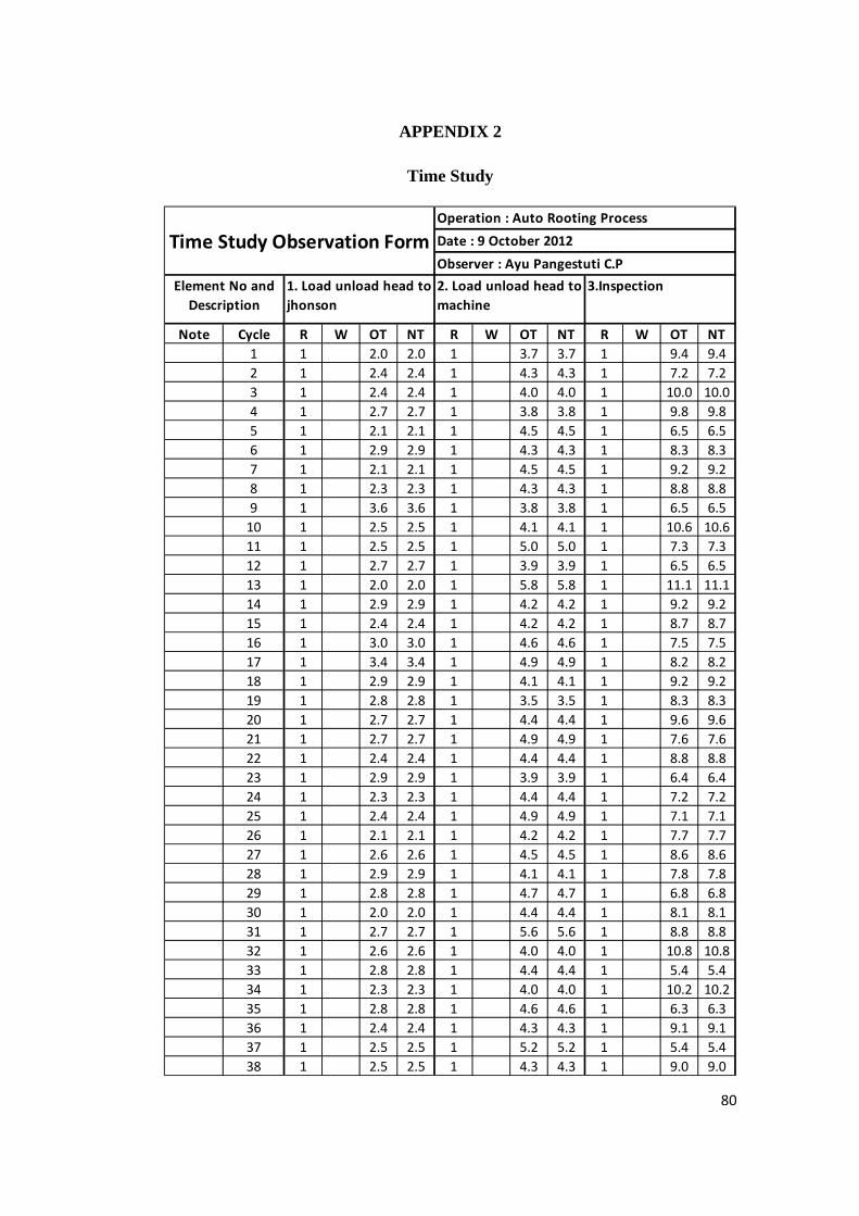
80
APPENDIX 2
Time Study
Note Cycle R W OT NT R W OT NT R W OT NT1 1 2.0 2.0 1 3.7 3.7 1 9.4 9.42 1 2.4 2.4 1 4.3 4.3 1 7.2 7.23 1 2.4 2.4 1 4.0 4.0 1 10.0 10.04 1 2.7 2.7 1 3.8 3.8 1 9.8 9.85 1 2.1 2.1 1 4.5 4.5 1 6.5 6.56 1 2.9 2.9 1 4.3 4.3 1 8.3 8.37 1 2.1 2.1 1 4.5 4.5 1 9.2 9.28 1 2.3 2.3 1 4.3 4.3 1 8.8 8.89 1 3.6 3.6 1 3.8 3.8 1 6.5 6.5
10 1 2.5 2.5 1 4.1 4.1 1 10.6 10.611 1 2.5 2.5 1 5.0 5.0 1 7.3 7.312 1 2.7 2.7 1 3.9 3.9 1 6.5 6.513 1 2.0 2.0 1 5.8 5.8 1 11.1 11.114 1 2.9 2.9 1 4.2 4.2 1 9.2 9.215 1 2.4 2.4 1 4.2 4.2 1 8.7 8.716 1 3.0 3.0 1 4.6 4.6 1 7.5 7.517 1 3.4 3.4 1 4.9 4.9 1 8.2 8.218 1 2.9 2.9 1 4.1 4.1 1 9.2 9.219 1 2.8 2.8 1 3.5 3.5 1 8.3 8.320 1 2.7 2.7 1 4.4 4.4 1 9.6 9.621 1 2.7 2.7 1 4.9 4.9 1 7.6 7.622 1 2.4 2.4 1 4.4 4.4 1 8.8 8.823 1 2.9 2.9 1 3.9 3.9 1 6.4 6.424 1 2.3 2.3 1 4.4 4.4 1 7.2 7.225 1 2.4 2.4 1 4.9 4.9 1 7.1 7.126 1 2.1 2.1 1 4.2 4.2 1 7.7 7.727 1 2.6 2.6 1 4.5 4.5 1 8.6 8.628 1 2.9 2.9 1 4.1 4.1 1 7.8 7.829 1 2.8 2.8 1 4.7 4.7 1 6.8 6.830 1 2.0 2.0 1 4.4 4.4 1 8.1 8.131 1 2.7 2.7 1 5.6 5.6 1 8.8 8.832 1 2.6 2.6 1 4.0 4.0 1 10.8 10.833 1 2.8 2.8 1 4.4 4.4 1 5.4 5.434 1 2.3 2.3 1 4.0 4.0 1 10.2 10.235 1 2.8 2.8 1 4.6 4.6 1 6.3 6.336 1 2.4 2.4 1 4.3 4.3 1 9.1 9.137 1 2.5 2.5 1 5.2 5.2 1 5.4 5.438 1 2.5 2.5 1 4.3 4.3 1 9.0 9.0
Time Study Observation FormOperation : Auto Rooting ProcessDate : 9 October 2012Observer : Ayu Pangestuti C.P
Element No and Description
1. Load unload head to jhonson
2. Load unload head to machine
3.Inspection

81
39 1 2.4 2.4 1 5.2 5.2 1 7.8 7.840 1 2.4 2.4 1 3.8 3.8 1 9.0 9.041 1 3.2 3.2 1 4.0 4.0 1 7.8 7.842 1 2.7 2.7 1 4.3 4.3 1 8.1 8.143 1 2.6 2.6 1 4.4 4.4 1 8.5 8.544 1 2.3 2.3 1 5.3 5.3 1 6.6 6.645 1 3.2 3.2 1 4.7 4.7 1 9.5 9.546 1 3.0 3.0 1 4.8 4.8 1 10.6 10.647 1 2.2 2.2 1 3.4 3.4 1 8.7 8.748 1 2.2 2.2 1 5.0 5.0 1 8.8 8.849 1 2.5 2.5 1 5.2 5.2 1 10.3 10.350 1 3.0 3.0 1 4.2 4.2 1 6.9 6.9
221.0
129.7
Average NT
Standard Time
2.6129.7
2.6
2.9
Total OTAverage OTTotal NT
Allowance 11.2%4.4
4.9
221.0SUMMARY
415.68.3
415.64.4
9.2
8.311.2% 11.2%
Time Study Observation FormOperation : Auto Rooting ProcessDate : 9 October 2012Observer : Ayu Pangestuti C.P
Element No and Description
1. Load unload head to jhonson
2. Load unload head to machine
3.Inspection

82
APPENDIX 3
Normality & Uniformity Test
By using MINITAB 14
Normality Test

83
Uniformity Test

84
By using manual calculation
OperationLoad unload head from jhonshon
Load unload head from machine
Inspect
1 2.0 3.7 9.42 2.4 4.3 7.23 2.4 4.0 10.04 2.7 3.8 9.85 2.1 4.5 6.56 2.9 4.3 8.37 2.1 4.5 9.28 2.3 4.3 8.89 3.6 3.8 6.510 2.5 4.1 10.611 2.5 5.0 7.312 2.7 3.9 6.513 2.0 5.8 11.114 2.9 4.2 9.215 2.4 4.2 8.716 3.0 4.6 7.517 3.4 4.9 8.218 2.9 4.1 9.219 2.8 3.5 8.320 2.7 4.4 9.621 2.7 4.9 7.622 2.4 4.4 8.823 2.9 3.9 6.424 2.3 4.4 7.225 2.4 4.9 7.126 2.1 4.2 7.727 2.6 4.5 8.628 2.9 4.1 7.829 2.8 4.7 6.830 2.0 4.4 8.131 2.7 5.6 8.832 2.6 4.0 10.833 2.8 4.4 5.434 2.3 4.0 10.235 2.8 4.6 6.3
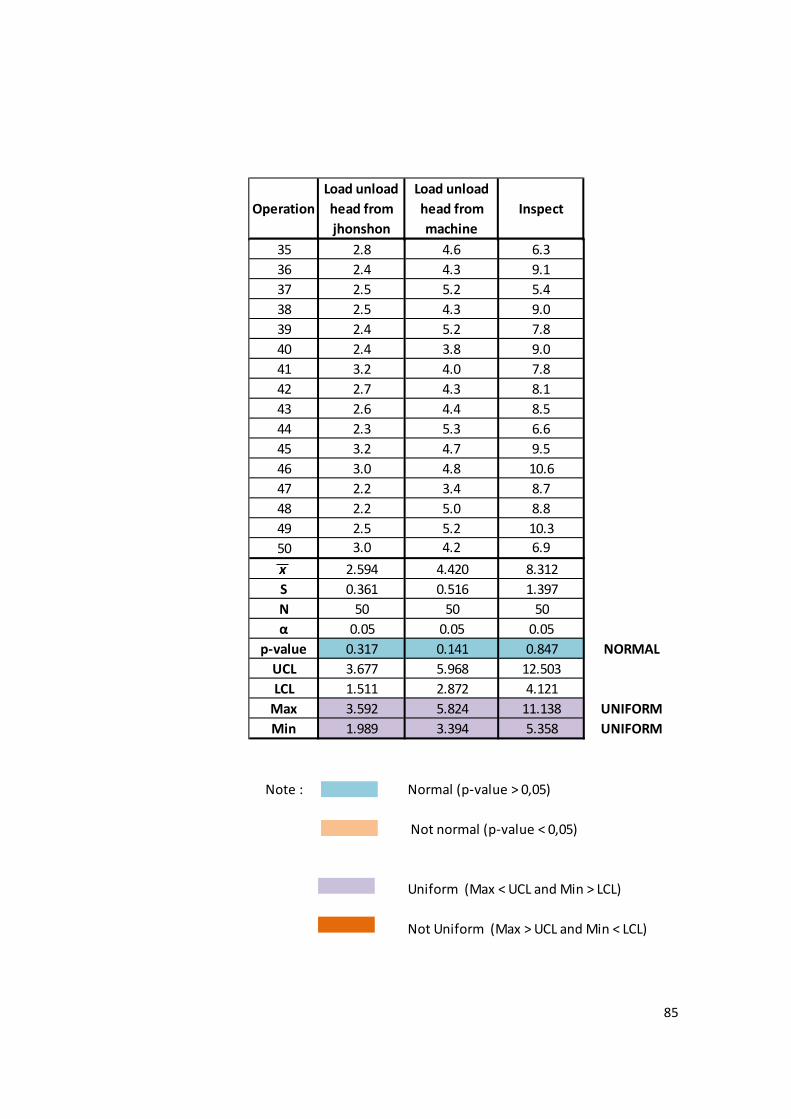
85
35 2.8 4.6 6.336 2.4 4.3 9.137 2.5 5.2 5.438 2.5 4.3 9.039 2.4 5.2 7.840 2.4 3.8 9.041 3.2 4.0 7.842 2.7 4.3 8.143 2.6 4.4 8.544 2.3 5.3 6.645 3.2 4.7 9.546 3.0 4.8 10.647 2.2 3.4 8.748 2.2 5.0 8.849 2.5 5.2 10.350 3.0 4.2 6.9x 2.594 4.420 8.312S 0.361 0.516 1.397N 50 50 50α 0.05 0.05 0.05
p-value 0.317 0.141 0.847 NORMALUCL 3.677 5.968 12.503LCL 1.511 2.872 4.121
Max 3.592 5.824 11.138 UNIFORMMin 1.989 3.394 5.358 UNIFORM
Note : Normal (p-value > 0,05)
Not normal (p-value < 0,05)
Uniform (Max < UCL and Min > LCL)
Not Uniform (Max > UCL and Min < LCL)
OperationLoad unload head from jhonshon
Load unload head from machine
Inspect

86
APPENDIX 4
Sufficiency Test
Operation
xi xi^2 xi xi^2 xi xi^21 2.0 4.0 3.7 13.5 9.4 88.02 2.4 6.0 4.3 18.4 7.2 51.33 2.4 5.8 4.0 15.7 10.0 99.54 2.7 7.4 3.8 14.5 9.8 96.25 2.1 4.6 4.5 20.3 6.5 42.96 2.9 8.7 4.3 18.2 8.3 68.57 2.1 4.4 4.5 20.0 9.2 84.98 2.3 5.1 4.3 18.6 8.8 77.99 3.6 12.9 3.8 14.1 6.5 41.910 2.5 6.4 4.1 16.9 10.6 111.611 2.5 6.3 5.0 25.2 7.3 53.312 2.7 7.3 3.9 15.1 6.5 41.913 2.0 4.0 5.8 33.9 11.1 124.014 2.9 8.2 4.2 17.4 9.2 84.915 2.4 5.8 4.2 18.0 8.7 75.716 3.0 9.1 4.6 20.8 7.5 55.717 3.4 11.3 4.9 23.7 8.2 67.618 2.9 8.2 4.1 16.8 9.2 85.519 2.8 7.9 3.5 12.1 8.3 69.520 2.7 7.4 4.4 19.5 9.6 92.021 2.7 7.3 4.9 24.4 7.6 57.222 2.4 5.7 4.4 19.6 8.8 77.823 2.9 8.5 3.9 15.4 6.4 41.024 2.3 5.1 4.4 19.6 7.2 52.025 2.4 5.7 4.9 23.6 7.1 49.826 2.1 4.4 4.2 17.4 7.7 58.727 2.6 6.9 4.5 20.7 8.6 74.728 2.9 8.2 4.1 16.9 7.8 60.729 2.8 8.0 4.7 22.4 6.8 45.730 2.0 4.0 4.4 19.8 8.1 65.931 2.7 7.4 5.6 31.3 8.8 78.232 2.6 6.6 4.0 16.3 10.8 116.133 2.8 7.9 4.4 19.0 5.4 29.434 2.3 5.2 4.0 16.2 10.2 104.635 2.8 8.0 4.6 21.6 6.3 39.6
Load unload head from jhonshon
Load unload head from machine
Inspect

87
36 2.4 5.9 4.3 18.2 9.1 82.037 2.5 6.1 5.2 27.2 5.4 28.738 2.5 6.1 4.3 18.1 9.0 80.239 2.4 5.6 5.2 26.5 7.8 60.540 2.4 5.7 3.8 14.8 9.0 81.641 3.2 10.1 4.0 16.0 7.8 61.642 2.7 7.4 4.3 18.8 8.1 66.343 2.6 6.6 4.4 19.7 8.5 72.244 2.3 5.3 5.3 27.7 6.6 43.445 3.2 10.0 4.7 21.9 9.5 90.446 3.0 9.2 4.8 22.9 10.6 112.447 2.2 4.7 3.4 11.5 8.7 75.648 2.2 4.9 5.0 25.2 8.8 77.849 2.5 6.3 5.2 27.2 10.3 106.550 3.0 9.1 4.2 17.5 6.9 48.0
∑ xi(∑ xi)^2∑ xi^2
NN'N' 31 22 45
30.27 21.56 44.6550 50 50
342.79 989.87 3551.4916821.34 48835.59 172753.53
129.70 220.99 415.64
OperationLoad unload head
from jhonshonLoad unload head
from machineInspect

88
APPENDIX 5
Simulation Model – Current Condition

89

90
TRACE
Load & unload head

91

92

93

94

95

96
DEBUG
Machine 1 - Load painted
head to Johnson wax
Machine 1 - Painted
head arrival
Machine 2 - Painted head
arrival
Machine 2 - Load painted
head to Johnson wax
Operation finish at rack
1
Machine 1 – Load painted
head to machine

97
Operation finish at rack
2
Machine 2 – Load painted
head to machine
Machine 1 – Running
Machine 2 – Running
Machine 1 - Painted head
arrival
Machine 1 - Load painted
head to Johnson wax

98
Machine 2 - Painted head
arrival
Machine 2 - Load painted
head to Johnson wax
Operation finish at rack
1
Operation finish at rack
2
Operation finish at
machine 1
Inspection process –
output machine 1

99
Machine 1 – Load painted
head to machine
Operation finish at
machine 2
Inspection process –
output machine 2
Machine 2 – Load painted
head to machine
Increase output
machine 1
Machine 1 – Running

100
Machine 2 – Running
Increase output
machine 2

101
APPENDIX 6
Simulation Model– Scenario 1: One Operator Handles Three Machines

102

103

104
APPENDIX 7
Simulation Model - Scenario 2: One Operator Handles Four Machines

105

106

107
APPENDIX 8
Simulation Model - Scenario 3: Two Operators Handle Seven Machines

108

109

110

111

112
APPENDIX 9
Critical Values for Student’s t Distribution

113
APPENDIX 10
Proposed System
Element Description Operator Machine 1 Machine 2 Machine 3
Time Idle Cum Time Idle Cum Time Idle Cum Time Idle Cum Load head to jhonson #1 1.3 1.3 0 1.3 0 1.3 0 1.3 Unload head from jhonson #1 1.3 2.6 0 1.3 0 1.3 0 1.3 Load head to machine #1 2.2 4.8 0 2.2 0 2.2 0 2.2 Move to #2 1 5.8 1 1 0 1 0 1 Load head to jhonson #2 1.3 7.1 1.3 2.3 0 1.3 0 1.3 Unload head from jhonson #2 1.3 8.4 1.3 3.6 0 1.3 0 1.3 Load head to machine #2 2.2 10.6 2.2 5.8 0 2.2 0 2.2 move to #3 1 11.6 1 6.8 1 1 0 1 Load head to jhonson #3 1.3 12.9 1.3 8.1 1.3 2.3 0 1.3 Unload head from jhonson #3 1.3 14.2 1.3 9.4 1.3 3.6 0 1.3 Load head to machine #3 2.2 16.4 2.2 11.6 2.2 5.8 0 2.2 Load head to jhonson #3 1.3 17.7 1.3 12.9 1.3 7.1 1.3 1.3 Move to #2 1 18.7 1 13.9 1 8.1 1 2.3 Load head to jhonson #2 1.3 20 1.3 15.2 1.3 9.4 1.3 3.6 Move to #1 1 21 1 16.2 1 10.4 1 4.6 Load head to jhonson #1 1.3 22.3 1.3 17.5 1.3 11.7 1.3 5.9 Unload head from jhonson #1 1.3 23.6 1.3 18.8 1.3 13 1.3 7.2

114
Element Description Operator Machine 1 Machine 2 Machine 3
Time Idle Cum Time Idle Cum Time Idle Cum Time Idle Cum IDLE 39.2 39.2 62.8 39.2 58 39.2 52.2 39.2 46.4 Unload head from machine #1 2.2 65 0 2.2 2.2 54.4 2.2 48.6 Load head to machine #1 2.2 67.2 0 2.2 2.2 56.6 2.2 50.8 Move to #2 1 68.2 1 1 1 57.6 1 51.8 Unload head from jhonson #2 1.3 69.5 1.3 2.3 1.3 58.9 1.3 53.1 Unload head from machine #2 2.2 71.7 2.2 4.5 0 2.2 2.2 55.3 Load head to machine #2 2.2 73.9 2.2 6.7 0 2.2 2.2 57.5 Move to #3 1 74.9 1 7.7 1 1 1 58.5 Unload head from jhonson #3 1.3 76.2 1.3 9 1.3 2.3 1.3 59.8 Unload head from machine #3 2.2 78.4 2.2 11.2 2.2 4.5 0 2.2 Load head to machine #3 2.2 80.6 2.2 13.4 2.2 6.7 0 2.2 Inspection #3 9.2 89.8 9.2 22.6 9.2 15.9 9.2 9.2 Load head to jhonson #3 1.3 91.1 1.3 23.9 1.3 17.2 1.3 10.5 Move to #2 1 92.1 1 24.9 1 18.2 1 11.5 Inspection #2 9.2 101.3 9.2 34.1 9.2 27.4 9.2 20.7 Load head to jhonson #2 1.3 102.6 1.3 35.4 1.3 28.7 1.3 22 Move to #1 1 103.6 1 36.4 1 29.7 1 23 Inspection #1 9.2 112.8 9.2 45.6 9.2 38.9 9.2 32.2 Load head to jhonson #1 1.3 114.1 1.3 46.9 1.3 40.2 1.3 33.5 Unload head to jhonson #1 1.3 115.4 1.3 48.2 1.3 41.5 1.3 34.8 IDLE 9.8 9.8 125.2 9.8 58 9.8 51.3 9.8 44.6 Unload head from machine #1 2.2 127.4 0 2.2 2.2 53.5 2.2 46.8 Load head to machine #1 2.2 129.6 0 2.2 2.2 55.7 2.2 49

115
Element Description Operator Machine 1 Machine 2 Machine 3
Time Idle Cum Time Idle Cum Time Idle Cum Time Idle Cum Move to #2 1 130.6 1 1 1 56.7 1 50 Unload head to jhonson #2 1.3 131.9 1.3 2.3 1.3 58 1.3 51.3 Unload head from machine #2 2.2 134.1 2.2 4.5 0 2.2 2.2 53.5 Load head to machine #2 2.2 136.3 2.2 6.7 0 2.2 2.2 55.7 Move to #3 1 137.3 1 7.7 1 1 1 56.7 Unload head from jhonson #3 1.3 138.6 1.3 9 1.3 2.3 1.3 58 Unload head from machine #3 2.2 140.8 2.2 11.2 2.2 4.5 0 2.2 Load head to machine #3 2.2 143 2.2 13.4 2.2 6.7 0 2.2 Inspection #3 9.2 152.2 9.2 22.6 9.2 15.9 9.2 9.2 Load head to jhonson #3 1.3 153.5 1.3 23.9 1.3 17.2 1.3 10.5 Move to #2 1 154.5 1 24.9 1 18.2 1 11.5 Inspection #2 9.2 163.7 9.2 34.1 9.2 27.4 9.2 20.7 Load head to jhonson #2 1.3 165 1.3 35.4 1.3 28.7 1.3 22 Move to #1 1 166 1 36.4 1 29.7 1 23 Inspection #1 9.2 175.2 9.2 45.6 9.2 38.9 9.2 32.2 Load head to jhonson #1 1.3 176.5 1.3 46.9 1.3 40.2 1.3 33.5 Unload head to jhonson #1 1.3 177.8 1.3 48.2 1.3 41.5 1.3 34.8 IDLE 9.8 9.8 187.6 9.8 58 9.8 51.3 9.8 44.6 Unload head from machine #1 2.2 189.8 0 2.2 2.2 53.5 2.2 46.8 Load head to machine #1 2.2 192 0 2.2 2.2 55.7 2.2 49 Move to #2 1 193 1 1 1 56.7 1 50 Unload head to jhonson #2 1.3 194.3 1.3 2.3 1.3 58 1.3 51.3 Unload head from machine #2 2.2 196.5 2.2 4.5 0 2.2 2.2 53.5

116
Element Description Operator Machine 1 Machine 2 Machine 3
Time Idle Cum Time Idle Cum Time Idle Cum Time Idle Cum Load head to machine #2 2.2 198.7 2.2 6.7 0 2.2 2.2 55.7 Move to #3 1 199.7 1 7.7 1 1 1 56.7 Unload head from jhonson #3 1.3 201 1.3 9 1.3 2.3 1.3 58 Unload head from machine #3 2.2 203.2 2.2 11.2 2.2 4.5 0 2.2 Load head to machine #3 2.2 205.4 2.2 13.4 2.2 6.7 0 2.2 Inspection #3 9.2 214.6 9.2 22.6 9.2 15.9 9.2 9.2 Load head to jhonson #3 1.3 215.9 1.3 23.9 1.3 17.2 1.3 10.5 Move to #2 1 216.9 1 24.9 1 18.2 1 11.5 Inspection #2 9.2 226.1 9.2 34.1 9.2 27.4 9.2 20.7 Load head to jhonson #2 1.3 227.4 1.3 35.4 1.3 28.7 1.3 22 Move to #1 1 228.4 1 36.4 1 29.7 1 23 Inspection #1 9.2 237.6 9.2 45.6 9.2 38.9 9.2 32.2 Load head to jhonson #1 1.3 238.9 1.3 46.9 1.3 40.2 1.3 33.5 Unload head to jhonson #1 1.3 240.2 1.3 48.2 1.3 41.5 1.3 34.8 IDLE 9.8 9.8 250 9.8 58 9.8 51.3 9.8 44.6 Unload head from machine #1 2.2 252.2 0 2.2 2.2 53.5 2.2 46.8 Load head to machine #1 2.2 254.4 0 2.2 2.2 55.7 2.2 49 Move to #2 1 255.4 1 1 1 56.7 1 50 Unload head to jhonson #2 1.3 256.7 1.3 2.3 1.3 58 1.3 51.3 Unload head from machine #2 2.2 258.9 2.2 4.5 0 2.2 2.2 53.5 Load head to machine #2 2.2 261.1 2.2 6.7 0 2.2 2.2 55.7 Move to #3 1 262.1 1 7.7 1 1 1 56.7 Unload head from jhonson #3 1.3 263.4 1.3 9 1.3 2.3 1.3 58

117
Element Description Operator Machine 1 Machine 2 Machine 3
Time Idle Cum Time Idle Cum Time Idle Cum Time Idle Cum Unload head from machine #3 2.2 265.6 2.2 11.2 2.2 4.5 0 2.2 Load head to machine #3 2.2 267.8 2.2 13.4 2.2 6.7 0 2.2 Inspection #3 9.2 277 9.2 22.6 9.2 15.9 9.2 9.2 Load head to jhonson #3 1.3 278.3 1.3 23.9 1.3 17.2 1.3 10.5 Move to #2 1 279.3 1 24.9 1 18.2 1 11.5 Inspection #2 9.2 288.5 9.2 34.1 9.2 27.4 9.2 20.7 Load head to jhonson #2 1.3 289.8 1.3 35.4 1.3 28.7 1.3 22 Move to #1 1 290.8 1 36.4 1 29.7 1 23 Inspection #1 9.2 300 9.2 45.6 9.2 38.9 9.2 32.2 Load head to jhonson #1 1.3 301.3 1.3 46.9 1.3 40.2 1.3 33.5 Unload head to jhonson #1 1.3 302.6 1.3 48.2 1.3 41.5 1.3 34.8 IDLE 9.8 9.8 312.4 9.8 58 9.8 51.3 9.8 44.6 Unload head from machine #1 2.2 314.6 0 2.2 2.2 53.5 2.2 46.8 Load head to machine #1 2.2 316.8 0 2.2 2.2 55.7 2.2 49 Move to #2 1 317.8 1 1 1 56.7 1 50 Unload head to jhonson #2 1.3 319.1 1.3 2.3 1.3 58 1.3 51.3 Unload head from machine #2 2.2 321.3 2.2 4.5 0 2.2 2.2 53.5 Load head to machine #2 2.2 323.5 2.2 6.7 0 2.2 2.2 55.7 Move to #3 1 324.5 1 7.7 1 1 1 56.7 Unload head from jhonson #3 1.3 325.8 1.3 9 1.3 2.3 1.3 58 Unload head from machine #3 2.2 328 2.2 11.2 2.2 4.5 0 2.2 Load head to machine #3 2.2 330.2 2.2 13.4 2.2 6.7 0 2.2 Inspection #3 9.2 339.4 9.2 22.6 9.2 15.9 9.2 9.2
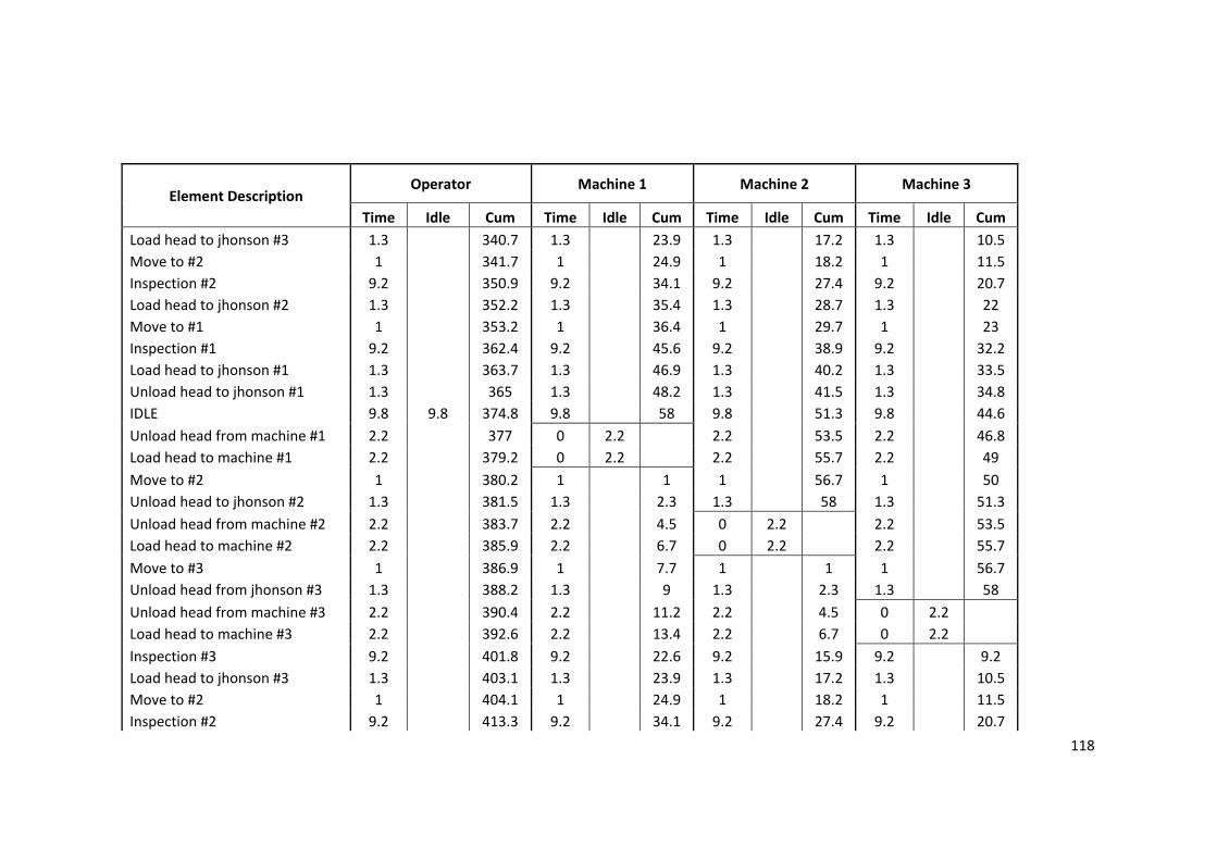
118
Element Description Operator Machine 1 Machine 2 Machine 3
Time Idle Cum Time Idle Cum Time Idle Cum Time Idle Cum Load head to jhonson #3 1.3 340.7 1.3 23.9 1.3 17.2 1.3 10.5 Move to #2 1 341.7 1 24.9 1 18.2 1 11.5 Inspection #2 9.2 350.9 9.2 34.1 9.2 27.4 9.2 20.7 Load head to jhonson #2 1.3 352.2 1.3 35.4 1.3 28.7 1.3 22 Move to #1 1 353.2 1 36.4 1 29.7 1 23 Inspection #1 9.2 362.4 9.2 45.6 9.2 38.9 9.2 32.2 Load head to jhonson #1 1.3 363.7 1.3 46.9 1.3 40.2 1.3 33.5 Unload head to jhonson #1 1.3 365 1.3 48.2 1.3 41.5 1.3 34.8 IDLE 9.8 9.8 374.8 9.8 58 9.8 51.3 9.8 44.6 Unload head from machine #1 2.2 377 0 2.2 2.2 53.5 2.2 46.8 Load head to machine #1 2.2 379.2 0 2.2 2.2 55.7 2.2 49 Move to #2 1 380.2 1 1 1 56.7 1 50 Unload head to jhonson #2 1.3 381.5 1.3 2.3 1.3 58 1.3 51.3 Unload head from machine #2 2.2 383.7 2.2 4.5 0 2.2 2.2 53.5 Load head to machine #2 2.2 385.9 2.2 6.7 0 2.2 2.2 55.7 Move to #3 1 386.9 1 7.7 1 1 1 56.7 Unload head from jhonson #3 1.3 388.2 1.3 9 1.3 2.3 1.3 58 Unload head from machine #3 2.2 390.4 2.2 11.2 2.2 4.5 0 2.2 Load head to machine #3 2.2 392.6 2.2 13.4 2.2 6.7 0 2.2 Inspection #3 9.2 401.8 9.2 22.6 9.2 15.9 9.2 9.2 Load head to jhonson #3 1.3 403.1 1.3 23.9 1.3 17.2 1.3 10.5 Move to #2 1 404.1 1 24.9 1 18.2 1 11.5 Inspection #2 9.2 413.3 9.2 34.1 9.2 27.4 9.2 20.7

119
Element Description Operator Machine 1 Machine 2 Machine 3
Time Idle Cum Time Idle Cum Time Idle Cum Time Idle Cum Load head to jhonson #2 1.3 414.6 1.3 35.4 1.3 28.7 1.3 22 Move to #1 1 415.6 1 36.4 1 29.7 1 23 Inspection #1 9.2 424.8 9.2 45.6 9.2 38.9 9.2 32.2 Load head to jhonson #1 1.3 426.1 1.3 46.9 1.3 40.2 1.3 33.5 Unload head to jhonson #1 1.3 427.4 1.3 48.2 1.3 41.5 1.3 34.8 IDLE 9.8 9.8 437.2 9.8 58 9.8 51.3 9.8 44.6 Unload head from machine #1 2.2 439.4 0 2.2 2.2 53.5 2.2 46.8 Load head to machine #1 2.2 441.6 0 2.2 2.2 55.7 2.2 49 Move to #2 1 442.6 1 1 1 56.7 1 50 Unload head to jhonson #2 1.3 443.9 1.3 2.3 1.3 58 1.3 51.3 Unload head from machine #2 2.2 446.1 2.2 4.5 0 2.2 2.2 53.5 Load head to machine #2 2.2 448.3 2.2 6.7 0 2.2 2.2 55.7 Move to #3 1 449.3 1 7.7 1 1 1 56.7 Unload head from jhonson #3 1.3 450.6 1.3 9 1.3 2.3 1.3 58 Unload head from machine #3 2.2 452.8 2.2 11.2 2.2 4.5 0 2.2 Load head to machine #3 2.2 455 2.2 13.4 2.2 6.7 0 2.2 Inspection #3 9.2 464.2 9.2 22.6 9.2 15.9 9.2 9.2 Load head to jhonson #3 1.3 465.5 1.3 23.9 1.3 17.2 1.3 10.5 Move to #2 1 466.5 1 24.9 1 18.2 1 11.5 Inspection #2 9.2 475.7 9.2 34.1 9.2 27.4 9.2 20.7 Load head to jhonson #2 1.3 477 1.3 35.4 1.3 28.7 1.3 22 Move to #1 1 478 1 36.4 1 29.7 1 23 Inspection #1 9.2 487.2 9.2 45.6 9.2 38.9 9.2 32.2

120
Element Description Operator Machine 1 Machine 2 Machine 3
Time Idle Cum Time Idle Cum Time Idle Cum Time Idle Cum Load head to jhonson #1 1.3 488.5 1.3 46.9 1.3 40.2 1.3 33.5 Unload head to jhonson #1 1.3 489.8 1.3 48.2 1.3 41.5 1.3 34.8 IDLE 9.8 9.8 499.6 9.8 58 9.8 51.3 9.8 44.6 Unload head from machine #1 2.2 501.8 0 2.2 2.2 53.5 2.2 46.8 Load head to machine #1 2.2 504 0 2.2 2.2 55.7 2.2 49 Move to #2 1 505 1 1 1 56.7 1 50 Unload head to jhonson #2 1.3 506.3 1.3 2.3 1.3 58 1.3 51.3 Unload head from machine #2 2.2 508.5 2.2 4.5 0 2.2 2.2 53.5 Load head to machine #2 2.2 510.7 2.2 6.7 0 2.2 2.2 55.7 Move to #3 1 511.7 1 7.7 1 1 1 56.7 Unload head from jhonson #3 1.3 513 1.3 9 1.3 2.3 1.3 58 Unload head from machine #3 2.2 515.2 2.2 11.2 2.2 4.5 0 2.2 Load head to machine #3 2.2 517.4 2.2 13.4 2.2 6.7 0 2.2 Inspection #3 9.2 526.6 9.2 22.6 9.2 15.9 9.2 9.2 Load head to jhonson #3 1.3 527.9 1.3 23.9 1.3 17.2 1.3 10.5 Move to #2 1 528.9 1 24.9 1 18.2 1 11.5 Inspection #2 9.2 538.1 9.2 34.1 9.2 27.4 9.2 20.7 Load head to jhonson #2 1.3 539.4 1.3 35.4 1.3 28.7 1.3 22 Move to #1 1 540.4 1 36.4 1 29.7 1 23 Inspection #1 9.2 549.6 9.2 45.6 9.2 38.9 9.2 32.2 Load head to jhonson #1 1.3 550.9 1.3 46.9 1.3 40.2 1.3 33.5 Unload head to jhonson #1 1.3 552.2 1.3 48.2 1.3 41.5 1.3 34.8 IDLE 9.8 9.8 562 9.8 58 9.8 51.3 9.8 44.6

121
Element Description Operator Machine 1 Machine 2 Machine 3
Time Idle Cum Time Idle Cum Time Idle Cum Time Idle Cum Unload head from machine #1 2.2 564.2 0 2.2 2.2 53.5 2.2 46.8 Load head to machine #1 2.2 566.4 0 2.2 2.2 55.7 2.2 49 Move to #2 1 567.4 1 1 1 56.7 1 50 Unload head to jhonson #2 1.3 568.7 1.3 2.3 1.3 58 1.3 51.3 Unload head from machine #2 2.2 570.9 2.2 4.5 0 2.2 2.2 53.5 Load head to machine #2 2.2 573.1 2.2 6.7 0 2.2 2.2 55.7 Move to #3 1 574.1 1 7.7 1 1 1 56.7 Unload head from jhonson #3 1.3 575.4 1.3 9 1.3 2.3 1.3 58 Unload head from machine #3 2.2 577.6 2.2 11.2 2.2 4.5 0 2.2 Load head to machine #3 2.2 579.8 2.2 13.4 2.2 6.7 0 2.2 Inspection #3 9.2 589 9.2 22.6 9.2 15.9 9.2 9.2 Load head to jhonson #3 1.3 590.3 1.3 23.9 1.3 17.2 1.3 10.5 Move to #2 1 591.3 1 24.9 1 18.2 1 11.5 Inspection #2 9.2 600.5 9.2 34.1 9.2 27.4 9.2 20.7 Load head to jhonson #2 1.3 601.8 1.3 35.4 1.3 28.7 1.3 22 Move to #1 1 602.8 1 36.4 1 29.7 1 23 Inspection #1 9.2 612 9.2 45.6 9.2 38.9 9.2 32.2 Load head to jhonson #1 1.3 613.3 1.3 46.9 1.3 40.2 1.3 33.5 Unload head to jhonson #1 1.3 614.6 1.3 48.2 1.3 41.5 1.3 34.8 IDLE 9.8 9.8 624.4 9.8 58 9.8 51.3 9.8 44.6 Unload head from machine #1 2.2 626.6 0 2.2 2.2 53.5 2.2 46.8 Load head to machine #1 2.2 628.8 0 2.2 2.2 55.7 2.2 49 Move to #2 1 629.8 1 1 1 56.7 1 50

122
Element Description Operator Machine 1 Machine 2 Machine 3
Time Idle Cum Time Idle Cum Time Idle Cum Time Idle Cum Unload head to jhonson #2 1.3 631.1 1.3 2.3 1.3 58 1.3 51.3 Unload head from machine #2 2.2 633.3 2.2 4.5 0 2.2 2.2 53.5 Load head to machine #2 2.2 635.5 2.2 6.7 0 2.2 2.2 55.7 Move to #3 1 636.5 1 7.7 1 1 1 56.7 Unload head from jhonson #3 1.3 637.8 1.3 9 1.3 2.3 1.3 58 Unload head from machine #3 2.2 640 2.2 11.2 2.2 4.5 0 2.2 Load head to machine #3 2.2 642.2 2.2 13.4 2.2 6.7 0 2.2 Inspection #3 9.2 651.4 9.2 22.6 9.2 15.9 9.2 9.2 Load head to jhonson #3 1.3 652.7 1.3 23.9 1.3 17.2 1.3 10.5 Move to #2 1 653.7 1 24.9 1 18.2 1 11.5 Inspection #2 9.2 662.9 9.2 34.1 9.2 27.4 9.2 20.7 Load head to jhonson #2 1.3 664.2 1.3 35.4 1.3 28.7 1.3 22 Move to #1 1 665.2 1 36.4 1 29.7 1 23 Inspection #1 9.2 674.4 9.2 45.6 9.2 38.9 9.2 32.2 Load head to jhonson #1 1.3 675.7 1.3 46.9 1.3 40.2 1.3 33.5 Unload head to jhonson #1 1.3 677 1.3 48.2 1.3 41.5 1.3 34.8 IDLE 9.8 9.8 686.8 9.8 58 9.8 51.3 9.8 44.6 Unload head from machine #1 2.2 689 0 2.2 2.2 53.5 2.2 46.8 Load head to machine #1 2.2 691.2 0 2.2 2.2 55.7 2.2 49 Move to #2 1 692.2 1 1 1 56.7 1 50 Unload head to jhonson #2 1.3 693.5 1.3 2.3 1.3 58 1.3 51.3 Unload head from machine #2 2.2 695.7 2.2 4.5 0 2.2 2.2 53.5 Load head to machine #2 2.2 697.9 2.2 6.7 0 2.2 2.2 55.7

123
Element Description Operator Machine 1 Machine 2 Machine 3
Time Idle Cum Time Idle Cum Time Idle Cum Time Idle Cum Move to #3 1 698.9 1 7.7 1 1 1 56.7 Unload head from jhonson #3 1.3 700.2 1.3 9 1.3 2.3 1.3 58 Unload head from machine #3 2.2 702.4 2.2 11.2 2.2 4.5 0 2.2 Load head to machine #3 2.2 704.6 2.2 13.4 2.2 6.7 0 2.2 Inspection #3 9.2 713.8 9.2 22.6 9.2 15.9 9.2 9.2 Load head to jhonson #3 1.3 715.1 1.3 23.9 1.3 17.2 1.3 10.5 Move to #2 1 716.1 1 24.9 1 18.2 1 11.5 Inspection #2 9.2 725.3 9.2 34.1 9.2 27.4 9.2 20.7 Load head to jhonson #2 1.3 726.6 1.3 35.4 1.3 28.7 1.3 22 Move to #1 1 727.6 1 36.4 1 29.7 1 23 Inspection #1 9.2 736.8 9.2 45.6 9.2 38.9 9.2 32.2 Load head to jhonson #1 1.3 738.1 1.3 46.9 1.3 40.2 1.3 33.5 Unload head to jhonson #1 1.3 739.4 1.3 48.2 1.3 41.5 1.3 34.8 IDLE 9.8 9.8 749.2 9.8 58 9.8 51.3 9.8 44.6 Unload head from machine #1 2.2 751.4 0 2.2 2.2 53.5 2.2 46.8 Load head to machine #1 2.2 753.6 0 2.2 2.2 55.7 2.2 49 Move to #2 1 754.6 1 1 1 56.7 1 50 Unload head to jhonson #2 1.3 755.9 1.3 2.3 1.3 58 1.3 51.3 Unload head from machine #2 2.2 758.1 2.2 4.5 0 2.2 2.2 53.5 Load head to machine #2 2.2 760.3 2.2 6.7 0 2.2 2.2 55.7 Move to #3 1 761.3 1 7.7 1 1 1 56.7 Unload head from jhonson #3 1.3 762.6 1.3 9 1.3 2.3 1.3 58 Unload head from machine #3 2.2 764.8 2.2 11.2 2.2 4.5 0 2.2

124
Element Description Operator Machine 1 Machine 2 Machine 3
Time Idle Cum Time Idle Cum Time Idle Cum Time Idle Cum Load head to machine #3 2.2 767 2.2 13.4 2.2 6.7 0 2.2 Inspection #3 9.2 776.2 9.2 22.6 9.2 15.9 9.2 9.2 Load head to jhonson #3 1.3 777.5 1.3 23.9 1.3 17.2 1.3 10.5 Move to #2 1 778.5 1 24.9 1 18.2 1 11.5 Inspection #2 9.2 787.7 9.2 34.1 9.2 27.4 9.2 20.7 Load head to jhonson #2 1.3 789 1.3 35.4 1.3 28.7 1.3 22 Move to #1 1 790 1 36.4 1 29.7 1 23 Inspection #1 9.2 799.2 9.2 45.6 9.2 38.9 9.2 32.2 Load head to jhonson #1 1.3 800.5 1.3 46.9 1.3 40.2 1.3 33.5 Unload head to jhonson #1 1.3 801.8 1.3 48.2 1.3 41.5 1.3 34.8 IDLE 9.8 9.8 811.6 9.8 58 9.8 51.3 9.8 44.6 Unload head from machine #1 2.2 813.8 0 2.2 2.2 53.5 2.2 46.8 Load head to machine #1 2.2 816 0 2.2 2.2 55.7 2.2 49 Move to #2 1 817 1 1 1 56.7 1 50 Unload head to jhonson #2 1.3 818.3 1.3 2.3 1.3 58 1.3 51.3 Unload head from machine #2 2.2 820.5 2.2 4.5 0 2.2 2.2 53.5 Load head to machine #2 2.2 822.7 2.2 6.7 0 2.2 2.2 55.7 Move to #3 1 823.7 1 7.7 1 1 1 56.7 Unload head from jhonson #3 1.3 825 1.3 9 1.3 2.3 1.3 58 Unload head from machine #3 2.2 827.2 2.2 11.2 2.2 4.5 0 2.2 Load head to machine #3 2.2 829.4 2.2 13.4 2.2 6.7 0 2.2 Inspection #3 9.2 838.6 9.2 22.6 9.2 15.9 9.2 9.2 Load head to jhonson #3 1.3 839.9 1.3 23.9 1.3 17.2 1.3 10.5

125
Element Description Operator Machine 1 Machine 2 Machine 3
Time Idle Cum Time Idle Cum Time Idle Cum Time Idle Cum Move to #2 1 840.9 1 24.9 1 18.2 1 11.5 Inspection #2 9.2 850.1 9.2 34.1 9.2 27.4 9.2 20.7 Load head to jhonson #2 1.3 851.4 1.3 35.4 1.3 28.7 1.3 22 Move to #1 1 852.4 1 36.4 1 29.7 1 23 Inspection #1 9.2 861.6 9.2 45.6 9.2 38.9 9.2 32.2 Load head to jhonson #1 1.3 862.9 1.3 46.9 1.3 40.2 1.3 33.5 Unload head to jhonson #1 1.3 864.2 1.3 48.2 1.3 41.5 1.3 34.8 IDLE 9.8 9.8 874 9.8 58 9.8 51.3 9.8 44.6 Unload head from machine #1 2.2 876.2 0 2.2 2.2 53.5 2.2 46.8 Load head to machine #1 2.2 878.4 0 2.2 2.2 55.7 2.2 49 Move to #2 1 879.4 1 1 1 56.7 1 50 Unload head to jhonson #2 1.3 880.7 1.3 2.3 1.3 58 1.3 51.3 Unload head from machine #2 2.2 882.9 2.2 4.5 0 2.2 2.2 53.5 Load head to machine #2 2.2 885.1 2.2 6.7 0 2.2 2.2 55.7 Move to #3 1 886.1 1 7.7 1 1 1 56.7 Unload head from jhonson #3 1.3 887.4 1.3 9 1.3 2.3 1.3 58 Unload head from machine #3 2.2 889.6 2.2 11.2 2.2 4.5 0 2.2 Load head to machine #3 2.2 891.8 2.2 13.4 2.2 6.7 0 2.2 Inspection #3 9.2 901 9.2 22.6 9.2 15.9 9.2 9.2
TOTAL IDLE TIME 166.6 61.6 61.6 61.6

1