DETERMINING THE ORBIT HEIGHT OF A LOW EARTH ORBITING ARTIFICIAL SATELLITE OBSERVED NEAR

THE LOCAL ZENITH by Michael A. Earl, Ottawa Centre (mikeearl@castor2.ca)

INTRODUCTION

hen you look up at satellites passing through your early evening (or early morning) sky, do you ever wonder how far away they are from you? You can determine the orbit height of a low Earth orbiting (LEO) artificial satellite by

using the satellite’s apparent travel when the satellite appears to be near your local zenith. Using the determined orbit height, you can also determine the approximate orbit period of the satellite.

W This method takes advantage of the fact that the satellite’s true velocity can be seen when it is nearly overhead, i.e. near your local zenith.

PRELIMINARY

When you stand near a highway and look at the cars passing by, do you ever notice that when a car is far away (in either direction), it does not appear to move very fast? Do you also notice that a car seems to move fastest when it is closest and just passing you? What you are experiencing is a simple example of vectors. When a car is far away, its velocity vector is directed nearly toward (or away from) you, so you cannot see a lot of motion. When a car is at its closest and just passing you, its velocity vector is exactly perpendicular to your line of sight, so what you see is the true velocity of the car and its fastest apparent motion.

Imagine a car traveling down a highway at a constant velocity v, and a person is observing that car’s travel. Figure 1 illustrates what the velocity vector is doing in this scenario.

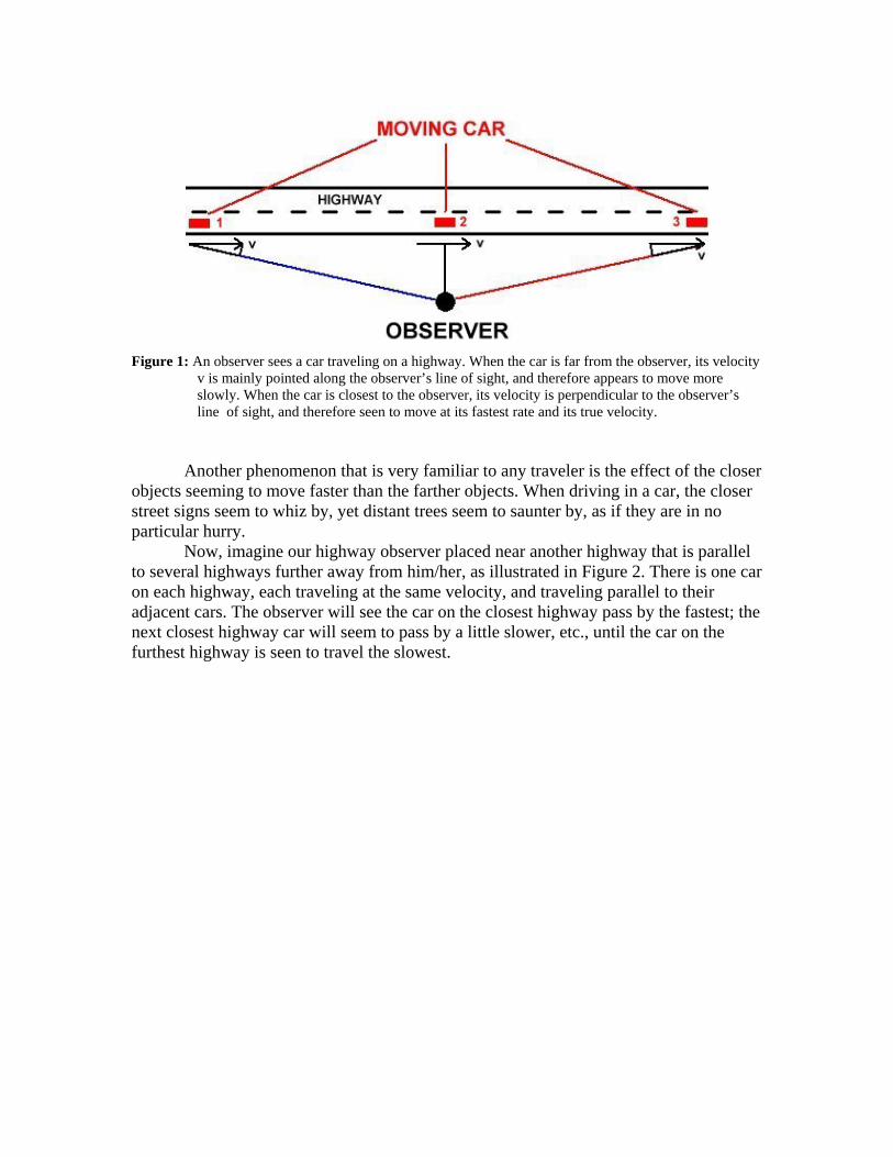
Figure 1: An observer sees a car traveling on a highway. When the car is far from the observer, its velocity

v is mainly pointed along the observer’s line of sight, and therefore appears to move more slowly. When the car is closest to the observer, its velocity is perpendicular to the observer’s line of sight, and therefore seen to move at its fastest rate and its true velocity.

Another phenomenon that is very familiar to any traveler is the effect of the closer objects seeming to move faster than the farther objects. When driving in a car, the closer street signs seem to whiz by, yet distant trees seem to saunter by, as if they are in no particular hurry. Now, imagine our highway observer placed near another highway that is parallel to several highways further away from him/her, as illustrated in Figure 2. There is one car on each highway, each traveling at the same velocity, and traveling parallel to their adjacent cars. The observer will see the car on the closest highway pass by the fastest; the next closest highway car will seem to pass by a little slower, etc., until the car on the furthest highway is seen to travel the slowest.

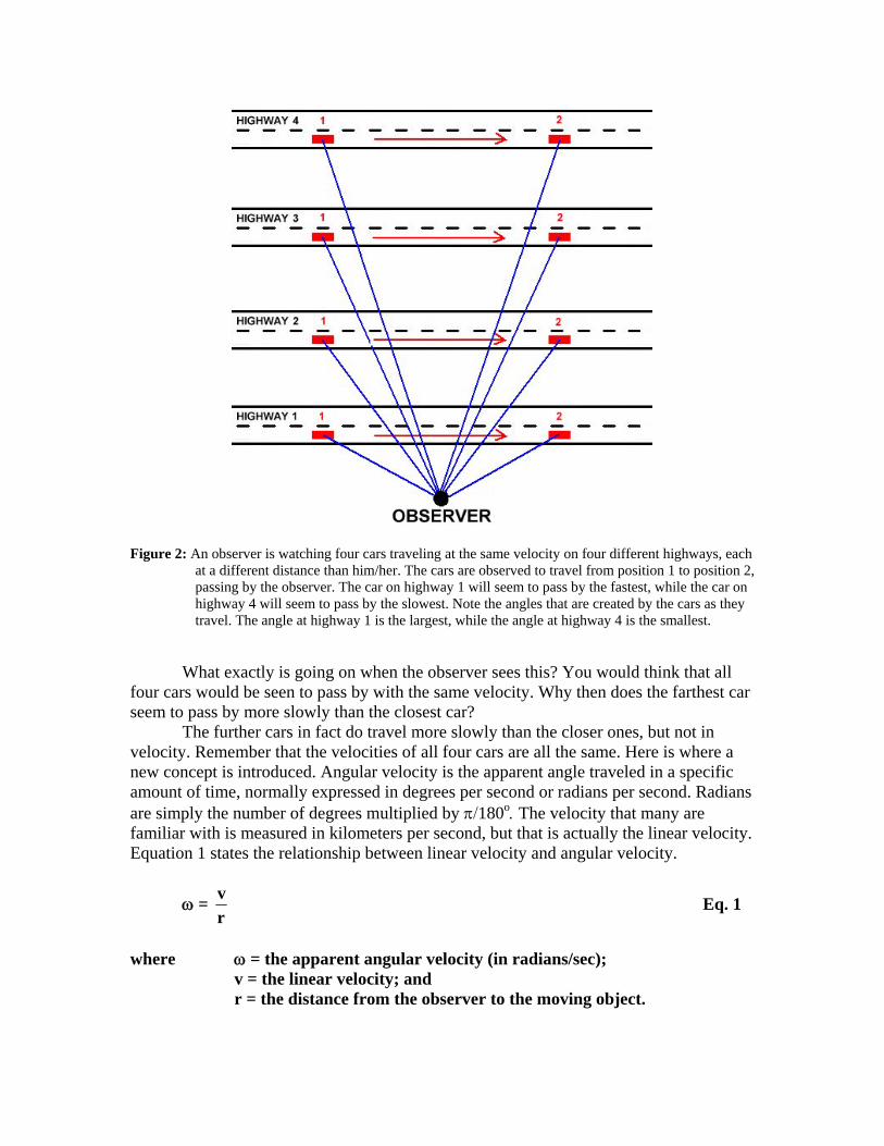
Figure 2: An observer is watching four cars traveling at the same velocity on four different highways, each at a different distance than him/her. The cars are observed to travel from position 1 to position 2, passing by the observer. The car on highway 1 will seem to pass by the fastest, while the car on highway 4 will seem to pass by the slowest. Note the angles that are created by the cars as they travel. The angle at highway 1 is the largest, while the angle at highway 4 is the smallest.

What exactly is going on when the observer sees this? You would think that all four cars would be seen to pass by with the same velocity. Why then does the farthest car seem to pass by more slowly than the closest car? The further cars in fact do travel more slowly than the closer ones, but not in velocity. Remember that the velocities of all four cars are all the same. Here is where a new concept is introduced. Angular velocity is the apparent angle traveled in a specific amount of time, normally expressed in degrees per second or radians per second. Radians are simply the number of degrees multiplied by π/180o. The velocity that many are familiar with is measured in kilometers per second, but that is actually the linear velocity. Equation 1 states the relationship between linear velocity and angular velocity.

ω = rv Eq. 1

where ω = the apparent angular velocity (in radians/sec); v = the linear velocity; and r = the distance from the observer to the moving object.

As the distance (r) increases, the apparent angular velocity (ω) decreases, for some linear velocity (v). This is what causes the more distant cars to appear to move more slowly than the closer cars. Watching a low Earth orbit satellite pass by in your evening sky is no different than looking at a car on the highway, except that the satellite highway is much further away and traces a very large circular (or nearly circular) road. The satellite analogy to the highway of Figure 1 is shown in Figure 3. The satellite analogy to the multiple highway concept of Figure 2 is shown in Figure 4.

Figure 3: The satellite equivalent of the highway analogy in Figure 1. When the satellite is further from the

observer, a large part of its velocity is pointed at or away from the observer, thus causing the satellite to appear to travel more slowly in the observer’s sky. As the satellite appears closer to the zenith (and decreasing in distance), the satellite appears to travel much faster, as the velocity becomes increasingly perpendicular to the observer’s line of sight. For a LEO satellite, the linear velocity (v) is approximately constant within its respective orbit.

Figure 4: Four satellites in four different orbits seen by an observer. In all four cases, each satellite crosses

the observer’s zenith. Unlike the example in Figure 2, the satellites will not have the same linearvelocity because of their four different orbit heights. As a result, the observed angular velocities will depend on both the satellites’ distances from the observer and the satellites’ linear velocities, as stated in Equation 1.

THEORY Now, imagine the observer at point P on the Earth observing a satellite S appearing near his/her zenith, as illustrated in Figure 5. The observer notes the apparent position of the satellite in his/her sky at two specific times.

Figure 5: An observer at point P sees a satellite S passing near his/her local zenith. He/she measures the

apparent angle the satellite travels θp, and divides it by the elapsed time Δt to determine the apparent angular velocity ωp. The angles have been exaggerated to better show the labels.

Once the observer measures the angle traveled (θp) in a specific time duration (Δt), the apparent angular velocity (ωp) can be determined using Equation 2.

ωp = tp

Δθ Eq. 2

where ωp = the angular velocity of the satellite seen by the observer at P; θp = the angle the satellite is observed to travel as seen at point P; and Δt = the elapsed time the satellite is seen to travel the angle θp. The satellite’s linear velocity (v) is the same with respect to both the observer (point P) and the center of the Earth (point C). This is exactly the same concept described in Figure 2.

v = ωph Eq. 3 where v = the linear velocity of the satellite; ωp = the apparent angular velocity of the satellite (in radians); and h = the height of the satellite above the Earth’s surface.

The height of the satellite (h) is the variable that needs to be solved. The distance from the center of the Earth to the satellite (rcs) is also dependent on the satellite’s linear velocity v through Kepler’s Third Law of Orbital Mechanics. Equation 4 simply states that the centripetal force acting on the satellite is equal to the gravitational force that the Earth exerts on it. This equation is always true for a perfectly circular orbit.

cs

2

rmv = 2

csrGMm Eq. 4

where m = the satellite’s mass; G = the Gravitational Constant; M = the Earth’s mass; and

rcs = the distance from the center of the Earth to the satellite. Simplifying Equation 4 leads to Equation 5.

v2 = csr

GM Eq. 5

Combining Equation 3 and Equation 5 gives us Equation 6.

v2 = csr

GM = ωp2h2 Eq. 6

so that:

ωp2h2 =

csrGM

Eq. 7

The distance rcs is not known. Since the satellite is near the observer’s zenith

however, we can take advantage of the fact that a line drawn from the center of the Earth (C) to the satellite (S) is nearly co-located with the line drawn from the observer (P) to the satellite. This is illustrated in Figure 6.

Figure 6: When observed at zenith, a satellite’s distance from an observer P and its height above the

Earth’s surface are identical. At zenith, the distance of the satellite from the Earth’s center C is the addition of the orbit height and the Earth’s radius at the point P.

When the satellite is observed very near the local zenith, its distance from the

observer and its height above the Earth’s surface are nearly identical. Therefore, the relationship described in Equation 8 can be used.

rcs = rcp + h Eq. 8

where rcp = the distance from the center of the Earth to the observer. Substituting for rcs using Equation 8:

ωp2h2 =

)hr(GM

cp + Eq. 9

So that: ωp

2h2rcp + ωp2h3 - GM = 0 Eq. 10

Finally,

h3 + rcph2 - 2p

GMω

= 0 Eq. 11

Equation 11 is known as a cubic equation and as a consequence the satellite orbit

height (h) will have three unique solutions. Two of the three solutions will be gibberish (which is slang for “not physically possible”), and therefore can be ignored. The solution that is left should be the correct and physically possible one.

Solving a cubic equation from scratch is not fun. If you thought the Quadratic Formula (that messy equation you learned, or at least tried to learn, in high school) was

bad, the Cubic Formula is even worse. Fortunately, the Internet has cubic equation solvers that automatically determine the solutions for you. See the References section to see the one that I used for this article. The coefficients for Equation 11 are:

A = 1; B = rcp; C = 0; and D = -GM / ωp

2

When plugging in these values, make sure that the units are correct. For rcp, I use

kilometers, for G, km3 / kg.s2, and for M, kilograms, so that I get kilometers for the answer’s units. Don’t forget the negative sign for the D coefficient either, or all three solutions will be gibberish!

PRACTICAL EXAMPLES

This would be the end of the article, except we need to test out theories using actual data before they can be taken as correct. For this reason, I set up my CCD camera, very much as illustrated in Figure 7, to capture satellites traveling through my local zenith. I used three different sites; Ottawa, Kemptville, and Brockville. On the evening of February 11, 2006, I set up my CCD camera in Ottawa, fitted with a 50mm lens to point directly at my local zenith, as shown in Figure 7.

Figure 7: My ST-9XE CCD camera mounted on a simple tripod. The CCD camera was fitted with a 50mm

lens and pointed at my local zenith with the aid of a simple bubble level. It caught LEO satellites as it continuously took images of the zenith with an 11.2 by 11.2 degree field of view.

From 7 p.m. to 9 p.m. E.S.T., February 11, 2006, the camera continuously captured 5 second exposures of my local zenith (yes, the sky was clear). I used the same method on May 27 and May 29, 2006, but using 10 second exposures. About 3000 images were collected in total. I sifted through these images, 20 images at a time, using blink comparator software to check for satellite streaks. I found 26 usable satellite streaks of differing lengths, and therefore differing heights. I used 2 of the 26 images as examples here, shown in Figure 8 and Figure 9.

EXAMPLE 1: SL-3 ROCKET BODY (#13771)

Figure 8: An image of a Russian SL-3 rocket body (#13771) that was captured by my ST-9XE’s CCD

camera pointed at my local zenith at 23:48:45 U.T.C. on February 11, 2006. The location of mylocal zenith at that time is denoted by the large red cross. The image FOV is about 11.2 by 11.2 degrees. North is at top, East is at left. The exposure time was 5 seconds.

I used the original image depicted in Figure 8 to determine the image scale of all images taken with the camera and the 50mm lens for future reference. I used 15 stars scattered throughout the image and plotted actual angular separation (in arc-minutes) between the stars vs. the pixel separation (in pixels) on the image for all combinations of two stars. I used a polynomial curve fitting technique to find the most accurate equation for the resultant graph. To make a long story short, the resultant image scale equation is stated in Equation 12.

θp = (-3 x 10-8) λ3 + (3 x 10-5) λ2 + 1.3154 λ + 0.2783 Eq. 12

where θp = angular separation between stars (in arc-minutes); and λ = the pixel separation between stars (in pixels).

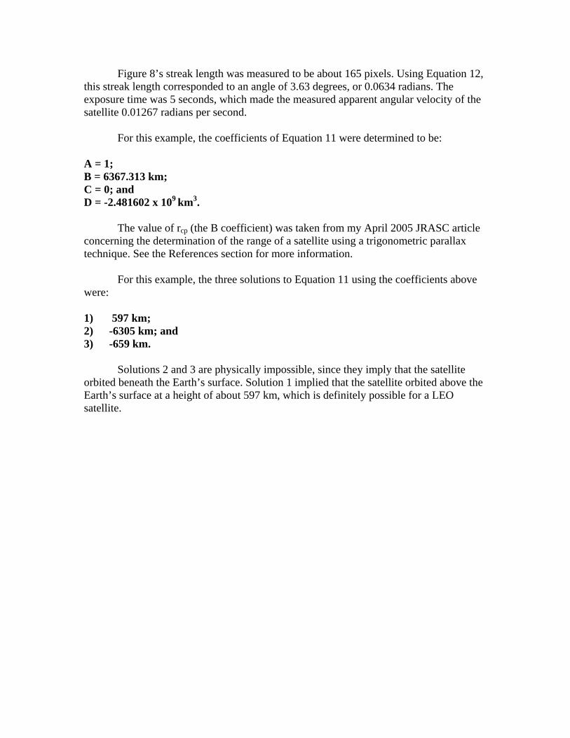
Figure 8’s streak length was measured to be about 165 pixels. Using Equation 12, this streak length corresponded to an angle of 3.63 degrees, or 0.0634 radians. The exposure time was 5 seconds, which made the measured apparent angular velocity of the satellite 0.01267 radians per second.

For this example, the coefficients of Equation 11 were determined to be:

A = 1; B = 6367.313 km; C = 0; and D = -2.481602 x 109

km3. The value of rcp (the B coefficient) was taken from my April 2005 JRASC article concerning the determination of the range of a satellite using a trigonometric parallax technique. See the References section for more information. For this example, the three solutions to Equation 11 using the coefficients above were: 1) 597 km; 2) -6305 km; and 3) -659 km.

Solutions 2 and 3 are physically impossible, since they imply that the satellite orbited beneath the Earth’s surface. Solution 1 implied that the satellite orbited above the Earth’s surface at a height of about 597 km, which is definitely possible for a LEO satellite.

EXAMPLE 2: MONITOR-E/SL-19 (#27840)

Figure 9: An image of a Russian Monitor-E/SL-19 satellite (#27840) captured at 00:15:16 U.T.C. February

12, 2006. The exposure time was 5 seconds, the same as in Example 1. The streak in this image is shorter than the one in Figure 4, implying that this satellite’s orbit height is larger than 597km.

The streak length in this image was measured to be about 123 pixels, which corresponded to an angle of 2.7 degrees, or 0.0474 radians. The exposure time was 5 seconds, which made the apparent angular velocity of the satellite 0.0095 radians per second. With this information, the coefficients became:

A = 1; B = 6367.313 km; C = 0; and D = -4.42946 x 109

km3.

Note that the only coefficient that changed between the first and second examples was the D coefficient. If the second measurement was performed on a different place on Earth, the B coefficient would have also changed, depending on the observation latitude.

The three solutions to Equation 11 using the coefficients above were:

1) 788 km; 2) -6254 km; and 3) -901 km.

Solutions 2 and 3 are physically impossible; therefore this satellite must have an orbit height of approximately 788 km. This result confirms it is higher up than the SL-3 rocket body’s 597 km height determined in Example 1.

ADDITIONAL MEASUREMENTS

I used this method on all the satellites I captured on that night (Table 1), and two future nights (Table 2). I tabulated the results in order of ascending measured orbit height to study the error behavior with respect to decreasing streak length. I also used two different exposure times, 5 and 10 seconds, to explore error behavior vs. streak length and orbit height. These are tabulated in Table 1 and Table 2 respectively. Table 3 was created to analyze other sources of error, such as orbit eccentricity and streak location in the image (angle from local zenith).

ID STREAK LENGTH

(pixels)

STREAK LENGTH

(rads)

D COEFFICIENT ( GM / ωp

2 )

HEIGHT (km)

TRUE HEIGHT

(km) PERIOD (min)

TRUE PERIOD

(min) 12465 177.912900 0.013677 -2.130869E+09 555 547 95.57 95.76 25527 169.434353 0.013024 -2.349776E+09 582 583 96.01 96.20 13771 164.878743 0.012673 -2.481590E+09 597 585 96.39 95.95 27840 123.328829 0.009477 -4.437512E+09 788 788 100.34 100.11 24968 120.503112 0.009260 -4.648144E+09 805 784 100.76 100.40 11111 113.216607 0.008700 -5.265847E+09 854 796 101.78 100.45 27433 105.304321 0.008092 -6.086907E+09 914 871 103.09 102.11 06154 94.810337 0.007286 -7.508461E+09 1009 953 105.07 104.53 25963 60.415230 0.004646 -1.846902E+10 1529 1418 116.40 114.08 25162 58.830264 0.004524 -1.947516E+10 1567 1471 117.21 115.23 09063 56.859948 0.004373 -2.084474E+10 1616 1499 118.30 115.17 25746 25.553865 0.001973 -1.024068E+11 3261 3013 156.71 148.48

Table 1: The determined orbit heights of 12 LEO satellites imaged in Ottawa, Ontario on February 11,

2006. The true height was obtained by using Software Bisque’s TheSky’s satellite orbit propagator (see the Software section below). The true period was obtained by taking the reciprocal of the mean motion value of the satellites’ orbit elements. The exposure time for each of these examples was 5 seconds. Each of the satellites was identified and correlated with the help of Software Bisque software (see the Software section below).

ID STREAK LENGTH

(pixels)

STREAK LENGTH

(rads)

D COEFFICIENT ( GM / ωp

2 )

HEIGHT (km)

TRUE HEIGHT

(km) PERIOD (min)

TRUE PERIOD

(min) 28651 317.971697 0.012235 -2.662660E+09 617 625 96.89 97.99 24966 243.977458 0.009383 -4.527491E+09 795 783 100.55 100.40 27597 241.238471 0.009277 -4.631089E+09 804 811 100.68 100.98 27421 234.079047 0.009001 -4.919286E+09 827 831 101.21 101.41 28051 235.586502 0.009059 -4.856413E+09 827 826 100.56 101.29 07734 232.038790 0.008923 -5.006343E+09 834 846 101.34 101.54 28888 198.406149 0.007627 -6.851340E+09 967 958 104.13 97.59 10731 197.344876 0.007586 -6.925351E+09 971 979 104.32 104.88 01314 140.174891 0.005386 -1.373795E+10 1335 1304 112.17 111.48 26083 123.422040 0.004742 -1.772324E+10 1501 1418 115.76 114.08 25771 122.298814 0.004699 -1.805041E+10 1513 1419 116.07 114.08 05104 119.104996 0.004576 -1.903177E+10 1550 1430 116.88 113.58 19195 112.538882 0.004324 -2.131788E+10 1632 1528 118.71 116.05 24829 98.600203 0.003789 -2.777030E+10 1840 1770 123.29 130.06

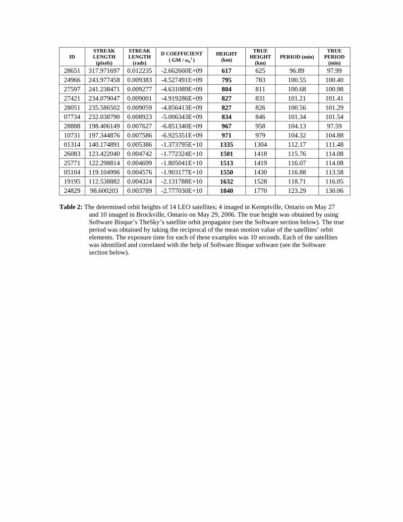
Table 2: The determined orbit heights of 14 LEO satellites; 4 imaged in Kemptville, Ontario on May 27

and 10 imaged in Brockville, Ontario on May 29, 2006. The true height was obtained by using Software Bisque’s TheSky’s satellite orbit propagator (see the Software section below). The true period was obtained by taking the reciprocal of the mean motion value of the satellites’ orbit elements. The exposure time for each of these examples was 10 seconds. Each of the satellites was identified and correlated with the help of Software Bisque software (see the Software section below).

ID TRUE

HEIGHT (km)

ORBIT ECCENTRICITY

STREAK LOCATION IN IMAGE

EXPOSURE TIME (sec)

HEIGHT ERROR

(km)

PERIOD ERROR

(min) 12465 547 0.0038 Far Left Center 5 8 -0.19 25527 583 0.00085 Top Left Corner 5 -1 -0.19 13771 585 0.0034 Left of Center 5 8 0.44 28651 625 0.0080 Top Left Corner 10 -8 -1.10 24966 783 0.00025 Top Right 10 12 0.15 24968 784 0.00025 Far Right Center 5 21 0.36 27840 788 0.0099 Bottom Right Corner 5 0 0.23 11111 796 0.0019 Top Left Corner 5 58 1.33 27597 811 0.000059 Bottom Right 10 -7 -0.30 28051 826 0.00028 Top Center 10 1 -0.73 27421 831 0.00013 Bottom Left 10 -4 -0.20 07734 846 0.0012 Bottom Right 10 -12 -0.20 27433 871 0.0015 Far Right Center 5 43 0.98 06154 953 0.0059 Right of Center 5 56 0.54 28888 958 0.054 Far Right Center 10 9 6.54 10731 979 0.0025 Center 10 -8 -0.56 01314 1304 0.0029 Center 10 31 0.69 25963 1418 0.000067 Top Left Corner 5 111 2.32 26083 1418 0.00012 Top Center 10 83 1.68 25771 1419 0.000045 Center 10 94 1.99 05104 1430 0.0043 Top Left Corner 10 120 3.30 25162 1471 0.000066 Top Right Corner 5 96 1.98 09063 1499 0.0061 Left of Center 5 117 3.13 19195 1528 0.0024 Left of Center 10 104 2.66 24829 1770 0.082 Bottom Left 10 140 -6.77 25746 3013 0.024 Bottom Left Corner 5 248 8.23

Table 3: A comparison between the orbit height, orbit eccentricity, streak location in the image and

exposure time vs. the orbit height error and orbit period error. All the satellites that are listed in Table 1 and Table 2 are listed here in the order of their true orbit height at the time of their imaging.

CONCLUSIONS

It is evident by looking at Table 1 and Table 2 that the smaller the apparent angular velocity (streak length) was, the higher the orbit height error became. Note how the longer exposure time in Table 2 slightly remedies the height error for a specific range.

The image scale equation that I derived from the SL-3 rocket body image

(Equation 12) might be a significant source of error. I used angular separations of 50 pixels and larger to determine it and therefore it might be biased against the smaller angular separations, such as the smaller streaks. Solutions to this problem might be to re-determining the image scale equation using smaller angular separations between stars and

a larger amount of stars, using a CCD with a higher resolution, and/or increasing the exposure time for the lower apparent angular velocity satellites, giving a longer streak. It will not matter if the stars streak as well, as the image scale has already been determined from the image of the SL-3 rocket body. As long as the apparatus does not change (ST-9XE CCD with 50mm lens) the image scale should not change appreciably from night to night.

Another interesting trend is that the height error is always positive for those

heights 1000km or larger. This definitely indicates a particular error that is dominating, most probably the field scale bias. However, if the field scale was solely determined through linear regression, these large errors might have been much worse. Determining the field distortions in more depth might be a way of minimizing such a bias.

Table 3 is interesting, yet difficult to analyze. It nevertheless illustrates the many

factors that can add to the overall height error that will be experienced. For instance, the error due to orbit eccentricity seems to be particularly noticeable when the eccentricity is 0.05 or above, as with the case of #24829 and #28888. This is not surprising, as the higher the height becomes, the larger the orbit eccentricity is allowed to be. As Table 3 also illustrates, the zenith angle of the satellite can also have a noticeable effect. Those satellites that appear at the far corners of the image will have a slightly larger height error than those nearer the center (zenith). The height equation was derived assuming that the satellite was at zenith, so the further from zenith the satellite appears, the larger the error will become. In the 11.2 by 11.2 degree field of view used here, satellites can be detected as far as 6 degrees from the zenith (at the image corners).

Table 3 effectively illustrates an interesting effect when determining the causes of

error. The question that should arise after looking at this table should be; “How can these errors be isolated, and minimized?” The answer might not be so cut and dry, since, as with the case of orbit height vs. eccentricity, one cause of error can directly influence another.

No satellite that orbits the Earth has a perfectly circular orbit. Many LEOs

satellites simply have very low eccentricity orbits, as Table 3 implies. This means that the orbit height cannot be constant, and therefore there is still a small radial velocity component that is not accounted for. However, the small 5-second exposure times that I used would guarantee that the height of the satellites would be generally constant over that time. So, the height determined would be the height that the satellite would have at that particular time, and does not automatically mean that the satellite is constantly at that height. As a result, the determined orbit period might also be larger or smaller than the true value.

Increasing the exposure time to over 10 seconds might further improve the height

determination error, but this can make the imaging more difficult. Note that in order to determine the angular velocity of the satellite, both endpoints of the streak had to be present and clearly defined. If the exposure time is increased, most of the lowest orbit

satellites would be able to pass outside the FOV during the exposure time, thereby causing a streak with only one (or no) endpoints.

When all is said and done, this method is surprisingly accurate for the lower

orbiting LEO satellites (200km to 800km orbit heights), and can be made more accurate for the higher orbiting LEO satellites (800km to 4000km orbit heights) when required.

REFERENCES AKiTi.ca Cubic Equation Solver

www.akiti.ca/Quad3Deg.html Earl, M. “Determining the Range of an Artificial Satellite Using its Observed

Trigonometric Parallax” JRASC: Vol. 99, No. 2, p. 54 Gupta, R. ed. 2006, Observer’s Handbook, The Royal Astronomical Society of

Canada (University of Toronto Press: Toronto)

Space Track: The Source for Space Surveillance Data www.space-track.org/perl/login.pl (Authorized Account Required)

SOFTWARE

“SatSort” Version 2: Satellite TLE Sorting Software: Mike Earl “TheSky” Level IV, Version 5: Astronomy Software: Software Bisque (www.bisque.com) “CCDSoft” Version 5: CCD Camera Control and Image Analysis Software: Software Bisque (www.bisque.com)

Mr. Michael A. Earl has been an avid amateur astronomer for over 30 years, and

served the Ottawa RASC as both its Meeting Chair and its Vice President. He currently serves as the "Artificial Satellites" Coordinator and the Webmaster for the Ottawa Centre’s web site (ottawa.rasc.ca). He constructed the Canadian Automated Small Telescope for Orbital Research (CASTOR): the very first remotely controlled and automated optical satellite tracking facility in Canada. He is currently working on a second-generation CASTOR system geared toward the advanced amateur and professional astronomy communities. You are welcome to visit his new CASTOR optical satellite tracking web site at www.castor2.ca.