developing a handbook for construction equipment

DEVELOPING A HANDBOOK FOR CONSTRUCTION EQUIPMENT MANAGEMENT AND

IMPLEMENTATION

By

RUSSELL V. SEIGNIOUS

A REPORT PRESENTED TO THE GRADUATE COMMITTEE OF THE DEPARTMENT OF CIVIL ENGINEERING IN PARTIAL FULFILLMENT OF THE

REQUDREMENNTS FOR THE DEGREE OF MASTER OF ENGINEERING

UNIVERSITY OF FLORIDA

SUMMER 1999

DISTRIBUTION STATEMENT A: Approved for Public Release -

Distribution Unlimited jmO QUALITY INSPECTED 4

19990827 101

Table of contents

1. INTRODUCTION . 1

2. EQUIPMENT ECONOMICS 2

2.1. TIME VALUE OF MONEY 2 2.2. COMPOUND INTEREST FACTORS 2

2.2.1. Single Payment Factors 3 2.2.2. Uniform Series Factors 3

2.3. DEPRECIATION TECHNIQUES 6 2.3.1. Straight Line 6 2.3.2. Sum Of the Years Digit 7 2.3.3. Declining Balance. 8

3. COST OF EQUIPMENT 11

3.1. ELEMENTS OF EQUIPMENT COST 11 3.2. OWNERSHIP COSTS 11

3.2.1. Amortized Method 12 3.2.2. Average Annual Investment Method. 13

3.3. OPERATING COSTS 15 3.3.1. Fuel Costs 15 3.3.2. Lubrication Costs 16 3.3.3. Repair Costs 16 3.3.4. Tire Costs 17 3.3.5. Special Items 17 3.3.6. Operators Wages 18

3.4. SOURCES OF TABULATED EQUIPMENT COSTS 19 3.4.1. Army Corps of Engineers 19 3.4.2. Rental Rate Blue Book 20

4. SOIL PROPERTIES AND HANDLING 21

4.1. SOIL CONDITIONS 21 4.1.1. Bank Measure 21 4.1.2. Loose Measure 21 4.1.3. Compacted Measure 21

4.2. SOIL SWELL 22 4.3. SOIL SHRINKAGE 22 4.4. LOAD AND SHRINKAGE FACTORS 23 4.5. SPOILBANKS 24

5. PRODUCTIVITY 27

6. EXCAVATING EQUIPMENT 29

6.1. SHOVELS 29 6.2. BACKHOES 32 6.3. DRAGLINES 36

7. TRACTORS/DOZERS 40

8. LOADERS 44

9. HAULING EQUEPMENT 48

9.1. ROLLING RESISTANCE 48 9.2. GRADE RESISTANCE 49 9.3. EFFECTIVE GRADE 49 9.4. SCRAPERS 49 9.5. PUSH LOADING 55 9.6. TRUCKS 59

10. EQUIPMENT SELECTION 61

10.1. LINE OF BALANCE 61

11. REFERENCES 65

APPENDIX A - COMPOUND INTEREST TABLES 66

1. Introduction Construction equipment may constitute one of the single largest long term capital

investments for a contractor. This is particularly true for those contractors engaged

primarily in horizontal construction. Regardless of the type of construction, the goal of

successful construction management is to complete projects in accordance with plans and

specifications, on time, within budget, and at the least possible cost. A crucial element in

accomplishing the aforementioned goal is the effective management and implementation of

construction equipment.

The fundamental goal of the equipment management process is to determine the

best piece of equipment for a given job. Although this is not necessarily a complex notion,

there are many factors to consider in making this determination. Most importantly, the

equipment must pay for itself. In other words, the cost to own and operate the equipment

must be less than what the equipment owner charges for its use. Today there exist many

different types of equipment that can accomplish the same job. Thus, the equipment

manager must typically consider more than one option.

Inefficient management of equipment can result in low production and/or idle

equipment; either of which can impact project duration and cost. Therefore, it is

important for contractors, construction managers, project managers, and any person

directly responsible for equipment management to be familiar with the methods leading to

selection of the appropriate equipment for a given job.

Not only is it important for equipment managers to be familiar with this subject, it

is also important for project owners, contract administrators, and others responsible for

representing the project owner. By being familiar with equipment cost formulation, the

owner's representative can more easily identify an inappropriate charge on a contract

action.

What this report sets forth to provide is a clear and concise handbook for the

equipment management process. It provides a basic overview of the subject and will allow

the reader to develop a construction equipment management process based on his or her

own set of criteria.

2. Equipment Economics

2.1. Time Value of Money It is an accepted fact that the value of money varies over time. Simply put, one

dollar today will have more buying power than one dollar ten years from today. Similarly,

one dollar deposited in a interest bearing savings account will grow to some value greater

than one dollar in the future. Because the value of money changes over time, it is

important for equipment managers to consider this time value of money when making

decisions on different equipment options. By reviewing the economic impacts of each

option the equipment manager can ensure the least expensive option is chosen. He does

this by developing equivalence models for each option. Equivalence is a concept that

looks at the value of two different options and determines the equivalent value of each

option based on interest and number of payments. For example; $1,000 is deposited in an

account earning 10% per year, so the value ofthat account at the end of the first year will

be $1,100. Therefore, it is said that $1,000 today is equivalent to $1,100 one year from

today, provided the interest rate is 10%.

2.2. Compound Interest Factors Compound interest factors are obtained from simple mathematical formulas.

These factors provide a simple means for analyzing economic alternatives to determine

equivalence. Most economic texts have tables with compound interest factors in tabulated

form. Appendix 1 of this report contains compound interest tables for convenience.

The following notations will be used in the compound interest factors to be

discussed subsequently:

P = The present value of a sum of money. For example: equipment purchase price, loan amount, down payment etc.

A = A uniform series of end of period payments. Loan payments are an example.

F = A future sum of money. n = The number of interest periods. /' = The interest rate per period.

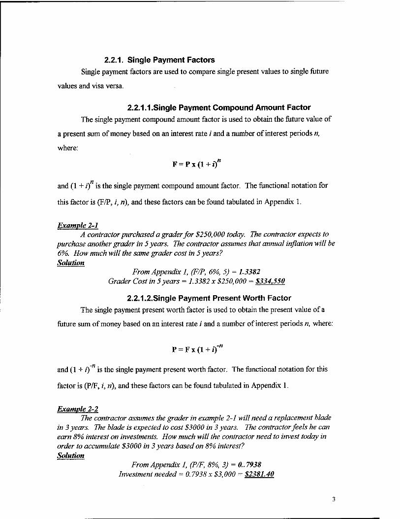
2.2.1. Single Payment Factors Single payment factors are used to compare single present values to single future

values and visa versa.

2.2.1.I.Single Payment Compound Amount Factor The single payment compound amount factor is used to obtain the future value of

a present sum of money based on an interest rate /' and a number of interest periods n,

where:

F = P x (1 + if

and (1+0 is the single payment compound amount factor. The functional notation for

this factor is (F/P, /', ri), and these factors can be found tabulated in Appendix 1.

Example 2-1 A contractor purchased a grader for $250,000 today. The contractor expects to

purchase another grader in 5 years. The contractor assumes that annual inflation will be 6%. How much will the same grader cost in 5 years? Solution

From Appendix 1, (F/P, 6%, 5) = 1.3382 Grader Cost in 5 years = 1.3382 x $250,000 = $334,550

2.2.1.2.Single Payment Present Worth Factor The single payment present worth factor is used to obtain the present value of a

future sum of money based on an interest rate /' and a number of interest periods n, where:

P = F x (1 + i)n

and (1 + /')" is the single payment present worth factor. The functional notation for this

factor is (P/F, i, n), and these factors can be found tabulated in Appendix 1.

Example 2-2 The contractor assumes the grader in example 2-1 will need a replacement blade

in 3 years. The blade is expected to cost $3000 in 3 years. The contractor feels he can earn 8% interest on investments. How much will the contractor need to invest today in order to accumulate $3000 in 3 years based on 8% interest? Solution

From Appendix 1, (P/F, 8%, 3) = ft. 7938 Investment needed = 0.7938 x $3,000 = $2381.40

2.2.2. Uniform Series Factors Uniform series factors are used to determine what a known uniform series of

payments future or present value will be. They are also used to determine what value of

uniform payment will result in a known present or future sum of money.

2.2.2.1.Uniform Series Capital Recovery Factor The uniform series capital recovery factor is used to obtain the series of equal

payments that are equal to a know present sum of money based on an interest rate / and a

number of interest periods n, where:

A = Yx[i(l + if]/[(l+if-l]

and [/(l + if]f[(l +if - 1] is the uniform series capital recovery factor. The functional

notation for this factor is (A/P, /, ri), and these factors can be found tabulated in Appendix

1.

Example 2-3 A contractor has found a used tractor with a price of $25,000. The contractor

wishes to finance this purchase. The bank offers a 5 year loan at 12% interest compounded annually with the payments due at the end of each year. What will the contractor's annual payments be? Solution

From Appendix 1, (A/P, 5, 12%) = 0.2774 Five annual payments = 0.2774 x $25,000 = $6,935

2.2.2.2.Uniform Series Present Worth Factor The uniform series present worth factor is used to obtain the present worth of a

series of known payments based on an interest rate /' and a number of interest periods n,

where:

p = AX[(i + ow-i]/['(i + 0"]

and [(1 + /')" - l]/[/(l + if] is the uniform series present worth factor. The functional

notation for this factor is (P/A, z, ri), and these factors can be found tabulated in Appendix

1.

2.2.2.3.Uniform Series Sinking Fund Factor

The uniform series sinking fond factor is used to obtain the uniform series of

investments required to accumulate a desired future sum of money base on an interest rate

/" and a number of interest periods n, where:

A = F xi/[(l +if-1]

and //[(l + if -1] is the uniform series sinking fond factor. The functional notation for

this factor is (A/F, /', ri), and these factors can be found tabulated in Appendix 1.

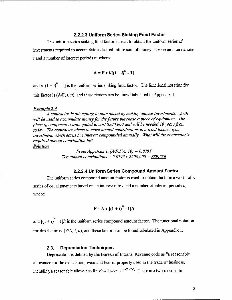
Example 2-4 A contractor is attempting to plan ahead by making annual investments, which

will be used to accumulate money for the future purchase apiece of equipment. The piece of equipment is anticipated to cost $500,000 and will be needed 10 years from today. The contractor elects to make annual contributions to a fixed income type investment, which earns 5% interest compounded annually. What will the contractor's required annual contribution be? Solution

From Appendix 1, (A/F,5%, 10) = 0.0795 Ten annual contributions = 0.0795 x $500,000 = $39,750

2.2.2.4.Uniform Series Compound Amount Factor

The uniform series compound amount factor is used to obtain the future worth of a

series of equal payments based on an interest rate / and a number of interest periods n,

where:

F = Ax[(l + i)"-l]/i

and [(1 + /') - l]/f is the uniform series compound amount factor. The functional notation

for this factor is (F/A, /', ri), and these factors can be found tabulated in Appendix 1.

2.3. Depreciation Techniques Depreciation is defined by the Bureau of Internal Revenue code as "a reasonable

allowance for the exhaustion, wear and tear of property used in the trade or business,

including a reasonable allowance for obsolescence."*2 ~2#6) There are two reasons for

depreciating equipment. The first reason is to establish you tax liability, and the second

reason is to determine the depreciation component of an equipment cost. It is legal to use

two different methods of depreciation for the two different reasons. Often owners will

elect to use the fastest depreciation technique, thus reducing the tax liability more quickly

over the first few years of an equipment's useful life. However, if the equipment is sold

for more than its depreciated book value, the excess will be treated as ordinary income and

taxed accordingly.

There are several methods of depreciation recognized by the Internal Revenue

Service. Three of the methods typically used for construction equipment are discussed in

detail subsequently. A graphical comparison of three of these methods is shown in Figure

2-1.

2.3.1. Straight Line

The straight line method of depreciation results in equal annual depreciation

amounts. The following formula is used to calculate straight line depreciation:

Dn = Initial Cost - Salva£e Value N

Where Dn = Depreciation for year in question N = Equipment life in years

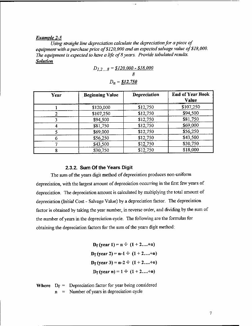
Example 2-5 Using straight line depreciation calculate the depreciation for apiece of

equipment with a purchase price of $120,000 and an expected salvage value of $18,000. The equipment is expected to have a life of 8 years. Provide tabulated results. Solution

Dlt2....8 = $120.000-$18.000 8

D„ = $12.750

Year Beginning Value Depreciation End of Year Book Value

1 $120,000 $12,750 $107,250

2 $107,250 $12,750 $94,500 3 $94,500 $12,750 $81,750 4 $81,750 $12,750 $69,000

5 $69,000 $12,750 $56,250

6 $56,250 $12,750 $43,500

7 $43,500 $12,750 $30,750

8 $30,750 $12,750 $18,000

2.3.2. Sum Of the Years Digit The sum of the years digit method of depreciation produces non-uniform

depreciation, with the largest amount of depreciation occurring in the first few years of

depreciation. The depreciation amount is calculated by multiplying the total amount of

depreciation (Initial Cost - Salvage Value) by a depreciation factor. The depreciation

factor is obtained by taking the year number, in reverse order, and dividing by the sum of

the number of years in the depreciation cycle. The following are the formulas for

obtaining the depreciation factors for the sum of the years digit method:

Df (year 1) = n 4- (1 + 2....+n)

Df (year 2) = n-1 4- (1 + 2....+n)

Df (year 3) = n-2 4- (1 + 2....+n)

Df (year n) = 1 -r- (1 + 2....+n)

Where Df = Depreciation factor for year being considered n = Number of years in depreciation cycle

Example 2-6 Using the same information from Example 2-5 calculate depreciation using the

sum of the years digit method and tabulate results. Solution

Dfiyear l)=8+36 = 0.2222

Df(year 2) = 7+36 = 0.1944

Df(year 3) = 6+36 = 0.1667

Df(year 4) =5+36 = 0.1389

Df(year 5) =4+36 = 0.1111

Dfiyear 6) =3+36 = 0.0833

Dfiyear 7) =2+36 = 0.0556

Dfiyear 8) = 1+36 = 0.0278 D„=Dfx (Total Depreciation) =Dfx $102,000.00

Year Beginning Value

Depreciation Factor

Depreciation End of Year Book Value

1 $120,000.00 0.2222 $22,664.40 $97,335.60 2 $97,335.60 0.1944 $19,828.80 $77,506.80 3 $77,506.80 0.1667 $17,003.40 $60,503.40 4 $60,503.40 0.1389 $14,167.80 $46,335.60 5 $46,335.60 0.1111 $11,332.20 $35,003.40 6 $35,003.40 0.0833 $8,496.60 $26,506.80 7 $26,506.80 0.0556 $5,671.20 $20,835.60 8 $20,835.60 0.0278 $2,835.60 $18,000.00

2.3.3. Declining Balance The declining balance method of depreciation is similar to the sum of the years

digit method in that the highest levels of depreciation occur in the first few years of

depreciation. Unlike the sum of the years digit method, when using the declining balance

method, the depreciation amount for a given year is obtained by multiplying the book

value at the beginning of the year being considered by a depreciation factor. Depreciation

factors for declining balance depreciation are obtained from the following formula:

Df=DBf^N

Where Df =

DBf =

N -

Depreciation factor

Declining Balance Factor (2 = Double Declining, 3 4 = Quadruple Declining, etc.) Number of years in depreciation cycle

Triple Declining,

Although any declining balance factor can, in theory, be used for calculating

declining balance depreciation, the most common factor is the double declining balance

factor.

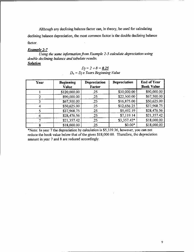
Example 2-7 Using the same information from Example 2-5 calculate depreciation using

double declining balance and tabulate results. Solution

Df=2+8 = 0.25 D„ = DfX Years Beginning Value

Year Beginning Value

Depreciation Factor

Depreciation End of Year Book Value

1 $120,000.00 .25 $30,000.00 $90,000.00 2 $90,000.00 .25 $22,500.00 $67,500.00 3 $67,500.00 .25 $16,875.00 $50,625.00 4 $50,625.00 .25 $12,656.25 $37,968.75 5 $37,968.75 .25 $9,492.19 $28,476.56 6 $28,476.56 .25 $7,119.14 $21,357.42 7 $21,357.42 .25 $3,357.42* $18,000.00 8 $18,000.00 .25 $0.00* $18,000.00

*Note: In year 7 the depreciation by calculation is $5,339.36, however, you can not reduce the book value below that of the given $18,000.00. Therefore, the depreciation amount in year 7 and 8 are reduced accordingly.

Figure 2-1 Comparison of Depreciation Methods

120000

3 (Q > o o ffi

100000 -

80000 -

60000 --

40000

20000

—I—

4

Year

■ Straight Line

■Double Declining

■SOYs Digit

10

3. Cost of Equipment

3.1. Elements of Equipment Cost There are two basic elements of equipment cost. These two elements are

ownership costs and operating costs. It is understood that your equipment must pay for

itself, therefore it is imperative that equipment owners accurately calculate ownership and

operating costs for their equipment. By accurately calculating these costs, the equipment

owner can confidently assign a cost that will result in the equipment being profitable.

Generally, ownership and operating costs are calculated based on an hourly rate.

The reason for calculating these costs on an hourly basis is because that is how they are

normally billed on construction projects.

3.2. Ownership Costs Ownership costs are those costs which the owner will incur regardless of whether

the equipment is used or not. Typical ownership costs are listed below.

• Depreciation • Interest (Investment, Cost of Capital) • Insurance • Taxes • Storage

The owner accounts for depreciation by knowing the purchase price and estimating a

salvage value and equipment useful life. The remaining items: interest, insurance, taxes,

and storage will be used to develop a minimum attractive rate of return. Minimum

attractive rate of return will be detailed in a subsequent example.

Interest is the cost resulting from borrowed money. The equipment owner should

account for this cost even if money is not borrowed, as the cash used to purchase the

equipment will no longer be available to earn interest in a savings or investment vehicle.

Insurance costs are for liability and equipment damage protection. Taxes covers those

costs associated with personal property taxes. Storage costs are for those times when the

equipment is not employed on a job.

11

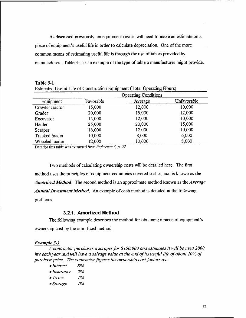
As discussed previously, an equipment owner will need to make an estimate on a

piece of equipment's useful life in order to calculate depreciation. One of the more

common means of estimating useful life is through the use of tables provided by

manufactures. Table 3-1 is an example of the type of table a manufacturer might provide.

Table 3-1 Estimated Useful Life of Construction Equipment (Total Operating Hours)

Operating Conditions Equipment Favorable Average Unfavorable

Crawler tractor 15,000 12,000 10,000 Grader 20,000 15,000 12,000 Excavator 15,000 12,000 10,000 Hauler 25,000 20,000 15,000 Scraper 16,000 12,000 10,000 Tracked loader 10,000 8,000 6,000 Wheeled loader 12,000 10,000 8,000 Data for this table was extracted from Reference 6, p. 27

Two methods of calculating ownership costs will be detailed here. The first

method uses the principles of equipment economics covered earlier, and is known as the

Amortized Method. The second method is an approximate method known as the Average

Annual Investment Method, An example of each method is detailed in the following

problems.

3.2.1. Amortized Method

The following example describes the method for obtaining a piece of equipment's

ownership cost by the amortized method.

Example 3-1 A contractor purchases a scraper for $150,000 attd estimates it will be used 2000

hrs each year and will have a salvage value at the end of its useful life of about 10% of purchase price. The contractor figures his ownership cost factors as:

• Interest 8% •Insurance 2% • Taxes 1% • Storage 1%

12

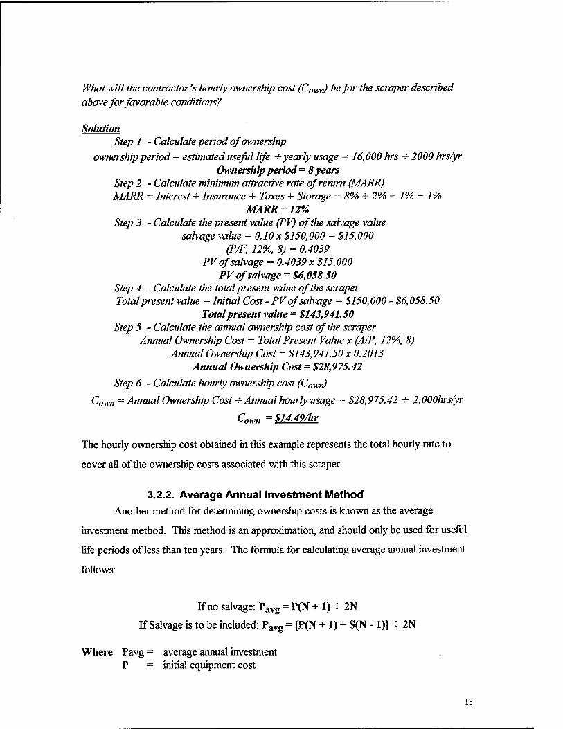
What will the contractor's hourly ownership cost (Cown) be for the scraper described above for favorable conditions?

Solution Step 1 - Calculate period of ownership

ownership period = estimated useful life +yearly usage = 16,000 hrs -t- 2000 hrs/yr Ownership period = 8 years

Step 2 - Calculate minimum attractive rate of return (MARR) MARR = Interest + Insurance + Taxes + Storage = 8% + 2% + 1% + 1%

MARR = 12% Step 3 - Calculate the present value (PV) of the salvage value

salvage value = 0.10x $150,000 = $15,000 (P/F, 12%, 8) = 0.4039

PV of salvage = 0.4039 x $15,000 PV of salvage = $6,058.50

Step 4 - Calculate the total present value of the scraper Total present value = Initial Cost - PV of salvage = $150,000 - $6,058.50

Total present value = $143,941.50 Step 5 - Calculate the annual ownership cost of the scraper

Annual Ownership Cost = Total Present Value x (A/P, 12%, 8) Annual Ownership Cost = $143,941.50 x 0.2013

Annual Ownership Cost = $28,975.42

Step 6 - Calculate hourly ownership cost (Cown)

Cown = Annual Ownership Cost + Annual hourly usage = $28,975.42 + 2,000hrs/yr

Cown =$14.49/hr

The hourly ownership cost obtained in this example represents the total hourly rate to

cover all of the ownership costs associated with this scraper.

3.2.2. Average Annual Investment Method Another method for determining ownership costs is known as the average

investment method. This method is an approximation, and should only be used for useful

life periods of less than ten years. The formula for calculating average annual investment

follows:

If no salvage: Pavg = P(N + 1) ■*• 2N

If Salvage is to be included: Pavg = [P(N + 1) + S(N - 1)] -5- 2N

Where Pavg^ average annual investment P = initial equipment cost

13

N = useful life in years S = salvage value

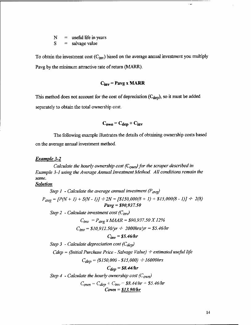
To obtain the investment cost (CjnV) based on the average annual investment you multiply

Pavg by the minimum attractive rate of return (MARR).

Ci„v = Pavg x MARR

This method does not account for the cost of depreciation (Cdep), so itmust be added

separately to obtain the total ownership cost.

C-own = C-dep + ^inv

The following example illustrates the details of obtaining ownership costs based

on the average annual investment method.

Example 3-2

Calculate the hourly ownership cost (Cown)for the scraper described in Example 3-1 using the Average Annual Investment Method. All conditions remain the same. Solution

Step 1 - Calculate the average annual investment (P^g)

Pavg = [P(N + 1) + S(N- 1)] + 2N = [$150,000(8 + 1) + $15,000(8 - 1)] -f- 2(8) Pavg = $90,937.50

Step 2 - Calculate investment cost (Cjm)

Q„v = PavgX MAAR = $90,937.50 X12%

Cinv = $10,912.50/yr -f- 2000hrs/yr = $5.46/hr

Qnv = $5.46/hr

Step 3 - Calculate depreciation cost (Cdep)

Cdep = (Initial Purchase Price - Salvage Value) -r- estimated useful life

Cdep = ($150,000-$15,000) -h 16000hrs

Cdep = $8.44/hr

Step 4 - Calculate the hourly ownership cost (Cown)

Cown = Cdep + Cinv = $8.44/hr + $5.46/hr Cown = $13.90/hr

14

The results of examples 3-1 and 3-2 show that these two methods differ only

slightly in the end result. That being the case, it should still be noted that the amortized

method is the more accurate of the two methods.

3.3. Operating Costs Operating costs are those costs that are incurred only when the equipment is in

use. One of the best sources for obtaining operating costs is historical data. Most

equipment manufacturers provide tables of adjustment factors to aid equipment owners in

estimating equipment operating costs. The following is a list of those items that are

generally considered operating costs.

• Fuel Costs • Lubrication Costs • Repair Costs • Tire Costs • Special Items • Operators Wages

The sum of these individual costs will represent the total operating cost of a piece

of equipment, and the sum of the total operating cost and total ownership cost will

represent the total equipment cost.

Total Equipment Cost = Total Ownership Costs + Total Operating Costs

3.3.1. Fuel Costs The cost of fuel will be obtained by multiplying a given piece of equipment's

hourly fuel burn in gallons per hour by the cost of fuel in dollars per gallon. A load factor

is usually applied to the basic fuel burn. Table 3-2 is an example of a fuel consumption

load factor table. Hourly fuel burn will be provided with most manufactures equipment

performance data. However, if fuel burn is unavailable the hourly fuel burn can be

estimated with the following formulas:

Gasoline Engines

Q = (0.7 x hp x load factor) -r- 6.2gph

15

Diesel Engines

Q = (0.5 x hp x load factor) 4- 7.2gph

Where Q = Fuel Burn (gallons per hour) hp = Equipment Horsepower

Table 3-2 Load Factors for Fuel Consumption

Operating Conditions

Equipment Favorable Average Severe Wheel Type, on pavement Wheel Type, off pavement Tracked Crawler Power Excavator

0.25 0.50 0.50 0.50

0.30 0.55 0.63 0.55

0.40 0.60 0.75 0.60

Data for this table was extracted from Reference 1, p. 33

Example 3-3 What would the estimated hourly cost of fuel be for a 30 horsepower diesel wheel

type loader used off road if the cost of diesel is $1.25/gallon and operating conditions are average? Solution

Step 1 - Calculate hourly fuel burn (O)

Q = (0.5xhpx load factor) 4- 7.2gph = (0.5x30x 0.55) 4- 7.2gph Q = 1.14gph

Step 2 - Calculate fuel cost per hour(Cfuei)

Cfuel = Q x Cost of fuel per gallon = 1.14gph x $1.25/gallon

Cfuei = $L42/hr

3.3.2. Lubrication Costs

Lubrication costs are those costs associated with equipment lubrication, hydraulic

fluids, oil filters, grease, etc.. Lubrication costs are best estimated from historical data.

Once enough historical data is obtained you can reduce lubrication costs to a percentage

of fuel costs.

3.3.3. Repair Costs

Repair costs are those cost associated with other than routine maintenance and

tires. Again, repair costs are best estimated from historical real data.

16

3.3.4. Tire Costs

Tire costs is not a negligible cost when it comes to heavy equipment. Replacing

four tires on a loader might cost upwards of $10,000. Hence, tire costs is an operating

cost element all its own. Tire life will vary widely based on the operating conditions,

therefore tire costs is somewhat difficult to estimate. As mentioned previously, historical

data is the best method for estimating tire life and costs. However, there are various

tables available for estimating tire life. Table 3-3 is an example of a tire life estimating aid.

Tire repair will add about 15% to tire replacement cost.*3"4945 The following equation can

be used to estimate tire cost:

Tire Cost ($/hr) = (Cost of set of tires) -^ (Estimated tire life)

Table 3-3 Typical Tire Life (hrs)

Operating Conditions

Equipment Favorable Average Severe Dozers and loaders 3,200 2,100 1,300 Motor graders 5,000 3,200 1,900 Scrapers

Conventional 4,600 3,300 2,500 Twin Engine 4,000 3,000 2,300 Push-pull and elevating 3,600 2,700 2,100

Trucks and wagons 3,500 2,100 1,100 Data for this table was extracted from Reference 3, p. 494

3.3.5. Special Items Special items represents the cost associated with high-wear items. Examples of

these type of items include, but are not limited to, scraper blade cutting edges and ripper

tips. Hourly costs for these items are calculated by simply dividing the cost of the item by

the expected life of the item.

17

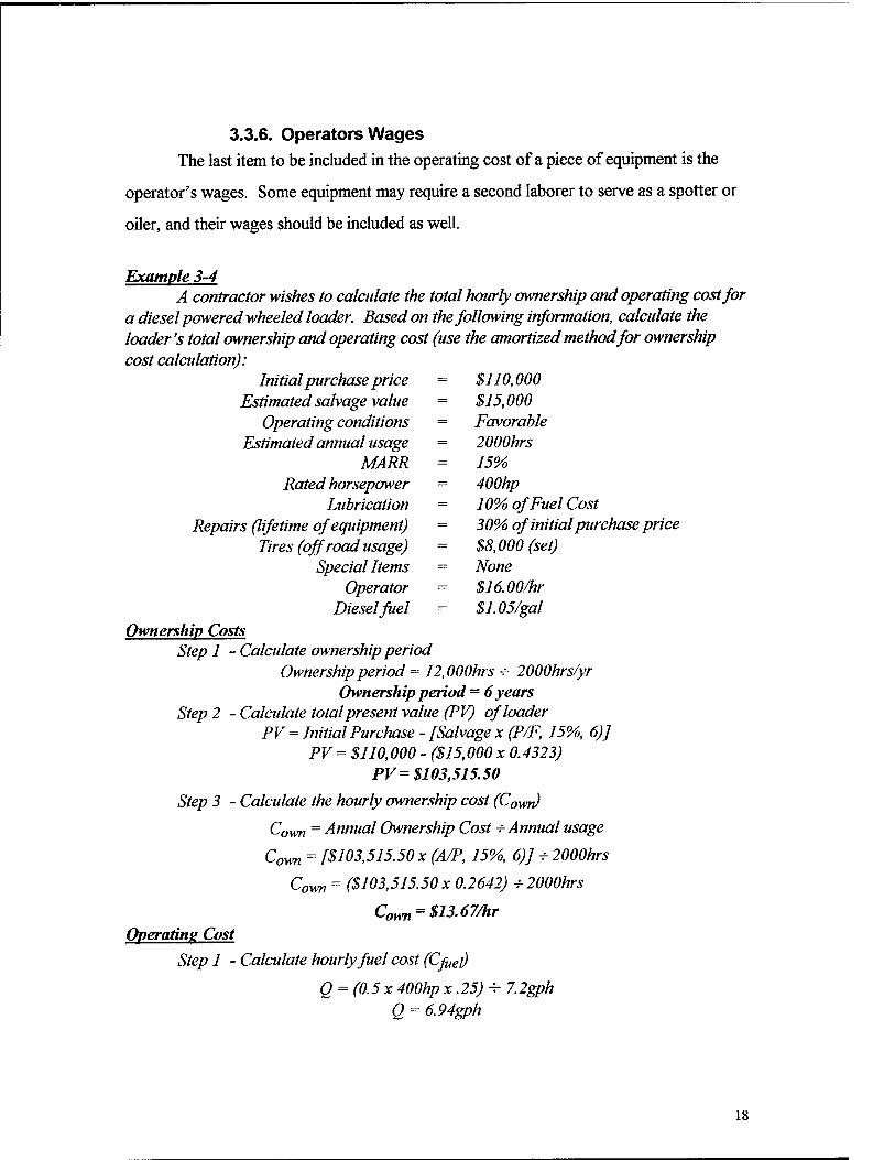
3.3.6. Operators Wages The last item to be included in the operating cost of a piece of equipment is the

operator's wages. Some equipment may require a second laborer to serve as a spotter or

oiler, and their wages should be included as well.

Example 3-4 A contractor wishes to calculate the total hourly ownership and operating cost for

a diesel powered wheeled loader. Based on the following information, calculate the loader's total ownership and operating cost (use the amortized method for ownership cost calculation):

Initial purchase price = $110,000 Estimated salvage value = $15,000

Operating conditions - Favorable Estimated annual usage = 2000hrs

MARR = 15% Rated horsepower = 400hp

Lubrication = 10% of Fuel Cost Repairs (lifetime of equipment) = 30% of initial purchase price

Tires (off road usage) = $8,000 (set) Special Items = None

Operator = $16.00/hr Diesel fuel = $1.05/gal

Ownership Costs Step 1 - Caladate ownership period

Ownership period = 12,000hrs + 2000hrs/yr Ownership period = 6 years

Step 2 - Calculate total present value (PV) of loader PV = Initial Purchase - [Salvage x (P/F, 15%, 6)]

PV = $110,000 - ($15,000 x 0.4323) PV= $103,515.50

Step 3 - Calculate the hourly ownership cost (Cown)

Cown = Annual Ownership Cost + Annual usage

Cown = [$103,515.50 x (A/P, 15%, 6)J +2000hrs

Cown = ($103,515.50x0.2642) +2000hrs

Cown = $13.67/hr Qperatins Cost

Step 1 - Calculate hourly fuel cost (Cfuei)

O = (0.5x 400hp x.25) + 7.2gph Q = 6.94gph

18

Cßel = 6.94gph x $1.05/gal

Cfuei = $7.29/hr

Step 2 - Calculate hourly lubrication cost (Ciuhe)

Qube = 0.10 x $7.29/hr = $. 73/hr

Step 3 - Calculate hourly repair cost (Crep)

Crep = (0.30 x $110,000) ■¥ 15,000hrs

Crep = $2.20/hr

Step 4 - Calculate hourly tire cost (Cfire)

Cure = $8,000 / 3,200hrs

Ctire = $2.50/hr

Step 5 - Calculate hourly operator wages (Cwage)

Cyi,age = $16.00/hr

Step 6 - Calculate total operating cost (Coper)

Coper ~ Cfuel + W«Z>e + Crep + Cfire + Cwage

Coper = S7.29 + $.73 + $2.20 + $2.50 + $16.00

C0peT = $28.72/hr Total equipment cost = Cown + Coper = $13.67 + $28.72 = $42.39/hr

3.4. Sources of Tabulated Equipment Costs There are several sources of tabulated equipment costs that equipment owners or

managers can use to obtain estimates of equipment ownership and operating costs. Two

sources that will be briefly discussed here, are the Army Corps of Engineers Construction

Equipment Ownership and Operating Expense Schedule and the Rental Rate Blue Book.

These two publications use different methods for obtaining their respective ownership and

operating costs. Thus, the rates in each will generally differ to some extent.

3.4.1. Army Corps of Engineers The Army Corps of Engineers Construction Equipment Ownership and Operating

Expense Schedule is published primarily for the use of government contracting agencies as

a guide to verifying and estimating contractor equipment charges on government projects.

This schedule attempts to represent, as realistically as possible, actual ownership and

operating costs. A review of this book reveals that the Army applies a discount to the list

price of equipment. This discount ranges from 7.5 % to 15% of list price. It is generally

19

accepted that contractors will receive some form of discount on equipment purchases, and

the Army attempts to reflect this in calculating the ownership portion of an equipment's .

cost. The Army Corps of Engineers Construction Equipment Ownership and Operating

Expense Schedule considers all those ownership and operating costs discussed previously

in this report with the exception of operator's wages.

3.4.2. Rental Rate Blue Book The Rental Rate Blue Book is published by Dataquest Incorporated. This book is

also a source of estimated ownership and operating cost for equipment. This publication

is somewhat conservative in comparison to the Army Corps of Engineers Construction

Equipment Ownership and Operating Expense Schedule, as evidenced by the fact the

manufacture's suggested list price is used in calculating the ownership cost of a piece of

equipment. In using the manufactures suggested list price, the resulting ownership cost

will typically be somewhat higher than what a contractor might actually incur in owning a

piece of equipment. As with the Army Corps of Engineers Construction Equipment

Ownership and Operating Expense Schedule, each of the ownership and operating costs

discussed previously in this report are considered in the Rental Rate Blue Book's

calculation of ownership and operating costs with the exception of operator's wages.

20

4. Soil Properties and Handling Heavy equipment in the construction industry is primarily employed in the

excavation, hauling, stabilization, loading, placing, grading, and finishing of material in the

earth's crust. This material consists primarily of soil and rock. Soil possesses some

unique characteristics that must be considered in selecting equipment that will most

efficiently carryout these tasks. Therefore, it is important that the equipment manager

have a basic understanding of these characteristics.

4.1. Soil Conditions Earthmoving material can be measured in three primary states. These states

include:

• Bank Measure • Loose Measure • Compacted Measure

4.1.1. Bank Measure Bank measure represents the volume of a soil before being disturbed. This is also

sometimes referred to as in-place or in-situ. This measure will typically be abbreviated as

BCY or BCM for bank cubic yard and bank cubic meter respectively.

4.1.2. Loose Measure Loose measure represents the volume of a disturbed soil, or one that has been

excavated or loaded. This measure will typically be abbreviated as LCY or LCM for loose

cubic yard and loose cubic meter respectively.

4.1.3. Compacted Measure Compacted measure represents the volume of a soil after it has been placed and

compacted. This measure will typically be abbreviated as CCY or CCM for compacted

cubic yard and compacted cubic meter respectively.

21

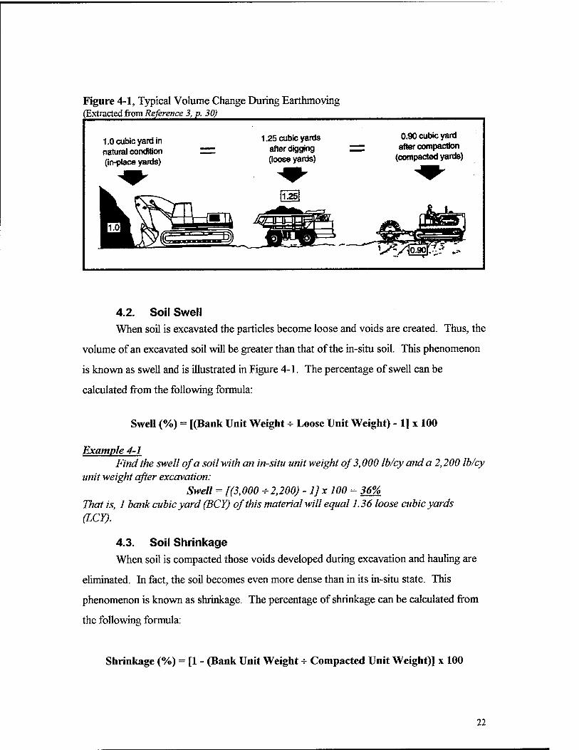
Figure 4-1, Typical Volume Change During Earthmoving (Extracted from Reference 3, p. 30)

1.0 cubic yard in natural condition (in-place yards)

1.25 cubic yards after digging (loose yards)

0.90 cubic yard after compaction

(compacted yards)

4.2. Soil Swell When soil is excavated the particles become loose and voids are created. Thus, the

volume of an excavated soil will be greater than that of the in-situ soil. This phenomenon

is known as swell and is illustrated in Figure 4-1. The percentage of swell can be

calculated from the following formula:

Swell (%) = [(Bank Unit Weight 4- Loose Unit Weight) - 1] x 100

Example 4-1 Find the swell of a soil with an in-situ unit weight of 3,000 Ib/cy and a 2,200 Ib/cy

unit weight after excavation: Swell = [(3,000 + 2,200) - 1]x 100 = 36%

That is, 1 bank cubic yard (BCY) of this material will equal 1.36 loose cubic yards (LCY).

4.3. Soil Shrinkage When soil is compacted those voids developed during excavation and hauling are

eliminated. In fact, the soil becomes even more dense than in its in-situ state. This

phenomenon is known as shrinkage. The percentage of shrinkage can be calculated from

the following formula:

Shrinkage (%) = [1 - (Bank Unit Weight - Compacted Unit Weight)] x 100

22

Example 4-2 Find the shrinkage of a soil with an in-situ unit weight of 2,800 Ib/cy and a 3,500

Ib/cy unit weight after compaction: Shrinkage = [1 - (2,800 +3,500)] x 100 = 20%

That is, 1 bank cubic yard (BCY) of this material will equal 0.80 compacted cubic yards (CCY).

4.4. Load and Shrinkage Factors It is often desirable to express earthmoving measures in a consistent measure,

often bank measure. Therefore, load and shrinkage factors were developed to make

converting between the three measures easier.

Haul units are often expressed in loose measure, therefore it is convenient to have

a factor for converting loose measure to bank measure. This factor is known as the load

factor and is expressed as follows:

Load Factor = Loose Unit Weight + Bank Unit Weight or

Load Factor = 1 + (1 + swell) and

Load Factor x Loose Measure = Bank Measure

A factor was also developed for converting bank measure to compacted measure,

and is known as the shrinkage factor. This factor is expressed as follows:

Shrinkage Factor = Bank Unit Weight + Compacted Unit Weight or

Shrinkage Factor = 1 - Shrinkage and

Shrinkage Factor x Bank Measure = Compacted Measure

Some typical soil volume characteristics, with respect to earthmoving operations, are

provided in Table 4-1.

Example 4-3 A soil has the following unit weights: 2,000 lb/LCY, 2,700 lb/BCY, and 3,400

Ib/CCY. (a) What is the load factor and shrinkage factor for this soil? (b) How many BCY's and CCY's will there be in 500,000 LCY's of this soil? Solution

(a) Load Factor = 2,000 + 2,700 = 0J4

Shrinkage Factor = 2,700 + 3,400 = 0.79 (b)

0.74 x 500. OOP LCY = 370.000 BCY 0.79 x 370,000 BCY = 292300 CCY

Table 4-1 Typical Soil Volume Change Characteristics*

Unit Weight (Ib/cy) Swell

(%) Shrinkage

(%) Load

Factor , Loose Bank Compacted Shrinkage

Factor

Clay 2310 Common Earth 2480 Rock (blasted) 3060 Sand and Gravel 2860

3000 3100 4600 3200

3750 3450 3550 3650

30 25 50 12

20 10

-30** 12

0.77 0.80 0.67 0.89

0.80 0.90

1.30** 0.88

*Exact Values vary with grain size distribution, moisture, compaction, and other factors. Tests are required to determine exact values for a specific soil. "Compacted rock, unlike soil, is less dense than in-place rock. Data for this table was extracted from Reference 3, p. 33

4.5. Spoil Banks It is often necessary to stockpile excavated material when performing earthmoving

operations. As a result, one must be able to determine the size of the expected stockpile

in order to determine an acceptable location for the stockpile. Stockpiled material can

either be in the form of a spoil bank or spoil pile. Spoil banks are triangular in cross

section and relatively long. Spoil piles are created when material is deposited from a fixed

position, and they are conical in shape. The size of a spoil bank or pile is governed by the

spoil material's angle of repose. Angle of repose is the angle measured from horizontal

that the sides of a spoil bank or pile will naturally form when deposited. Table 4-2 list

some common values for soil angle of repose.

24

Triangular Spoil Banks

Volume = Section Area x Length B = [(4V)-(LxtanR)]1/2

H = (B x tan R) - 2

Where B = base width H = pile height L = pile length R = angle of repose (deg) V = pile volume

Conical Spoil Piles Volume = 1/3 x Base area x Height

D = [(7.64V) * (tan R)]1/3

H = (D - 2) x tan R

Where D = Diameter of pile base

Table 4-2 Typical Values For Excavated Soil Angle of Repose

Material Angle of Repose (deg) Clay Common earth, dry Common earth, moist Gravel Sand, dry Sand, moist

35 32 37 35 25 37


Example 4-4 Find the base width and height of a spoil bank containing 100,000 BCY of

material. The length of the bank is 500 feet, and the material is clay. Solution

From Table 4-1 Swell for Clay = 30% From Table 4-2 Angle of repose for clay = 35° Step 1 - Calculate Loose Volume

Loose Volume = 1.3x 100,000BCYx27f?/yd? = 3.510,000 tf Step 2 - Calculate Base Width

Base Width = f(4 x 3,510,000) + (500 x tan 35 °)]m

Base Width = 200feet

25

Step 3 - Calculate Height Height = (200x tan 35°)

Height = 70 feet

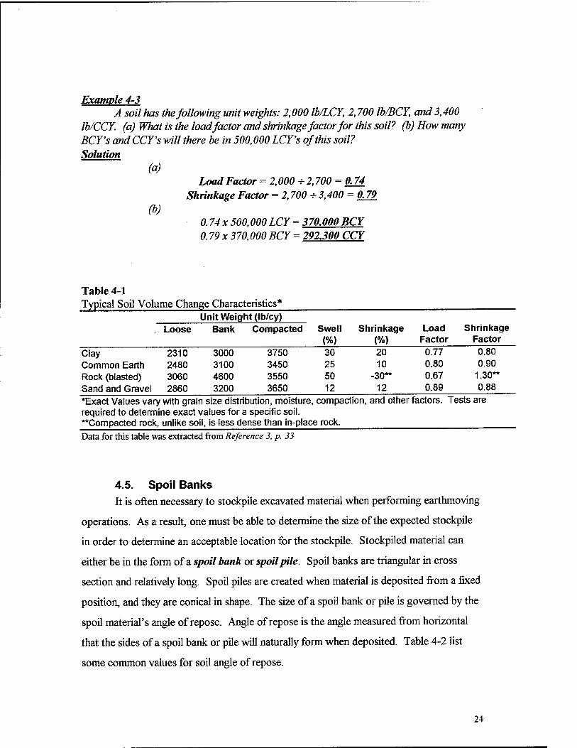
Example 4-4 Find the base diameter and height of a spoil pile containing 200 BCY of dry sand.

Solution From Table 4-1 Swell for sand = 12% From Table 4-2 Angle of repose for dry sand = 25° Step 1 - Calculate Loose Volume

Loose Volume = 1.12x 200 x 27f?/ya* = 6.048 ft Step 2 - Calculate Base Diameter

Base Diameter = [(7.64 x 6,048) + (tan 25 °)Jl/3

Base Diameter = 46 feet Step 3 - Calculate Height

Height = (46 + 2)x tan 25 ° Height = 10.7 feet

26

5. Productivity The production of any particular earthmoving operation consists of the following

elements:

• Loading • Hauling • Dumping • Return • Spot

Most of these terms are self explanatory with the possible exception of spot. Spot

represents the time necessary for a haul unit to maneuver into position for loading. These

elements represent the total production of a particular earthmoving activity. To calculate

the total production you must first be able to calculate the production of each individual

piece of equipment involved in the operation. The production of a piece of equipment is

based on cycle time and volumetric capacity of the equipment. Cycle time is the time

required of a given piece of equipment to complete one cycle of its intended operation.

Production can be calculated as:

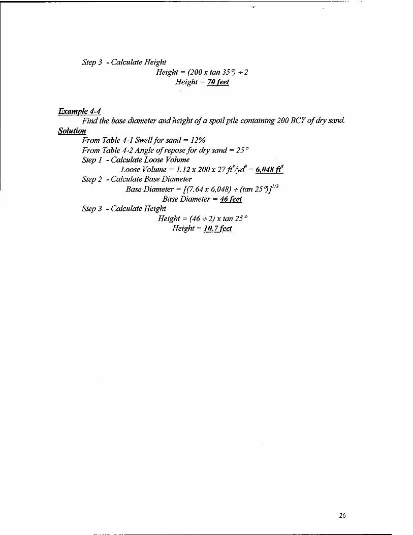
Production = volume per cycle x cycles per hour x efficiency factor

Because it is not possible to operate a piece of equipment at 100% efficiency, the

production is reduced by some efficiency factor. There are two ways of estimating an

efficiency factor. One method is to estimate the number of working minutes per hour, 50

minutes per hour or 0.833 is popular. The second method uses information obtained from

tables similar to Table 5-1. Regardless of the method used, efficiency is effected by

management conditions and job conditions.

Management Conditions Include: • worker skill, training, and motivation • selection, operation, and maintenance of equipment • planning, job layout, supervision, and coordination

27

Job Conditions Include: • topography and work dimensions • surface and weather conditions • work methods or sequence

Table 5-1 Efficiency Factors For Earthmoving Operations

Management Conditions Job Conditions Excellent Good Fair Poor Excellent 0.84 0.81 0.76 0.70 Good 0.78 0.75 0.71 0.65 Fair 0.72 0.69 0.65 0.60 Poor 0.63 0.61 0.57 0.52 Data for this table was extracted from Reference 3, p. 23

28

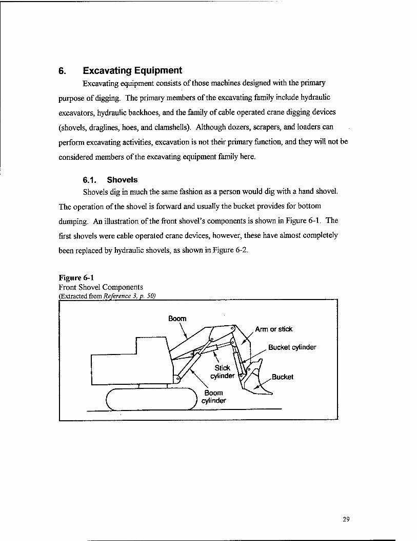
6. Excavating Equipment Excavating equipment consists of those machines designed with the primary

purpose of digging. The primary members of the excavating family include hydraulic

excavators, hydraulic backhoes, and the family of cable operated crane digging devices

(shovels, draglines, hoes, and clamshells). Although dozers, scrapers, and loaders can

perform excavating activities, excavation is not their primary function, and they will not be

considered members of the excavating equipment family here.

6.1. Shovels Shovels dig in much the same fashion as a person would dig with a hand shovel.

The operation of the shovel is forward and usually the bucket provides for bottom

dumping. An illustration of the front shovel's components is shown in Figure 6-1. The

first shovels were cable operated crane devices, however, these have almost completely

been replaced by hydraulic shovels, as shown in Figure 6-2.

Figure 6-1 Front Shovel Components Extracted from Reference 3, p. 50)

Boom

Stick A \U V cylinder Ppv

\ Boom ) cylinder

Arm or stick

Bucket cylinder

'S . Bucket I i

(

*s

29

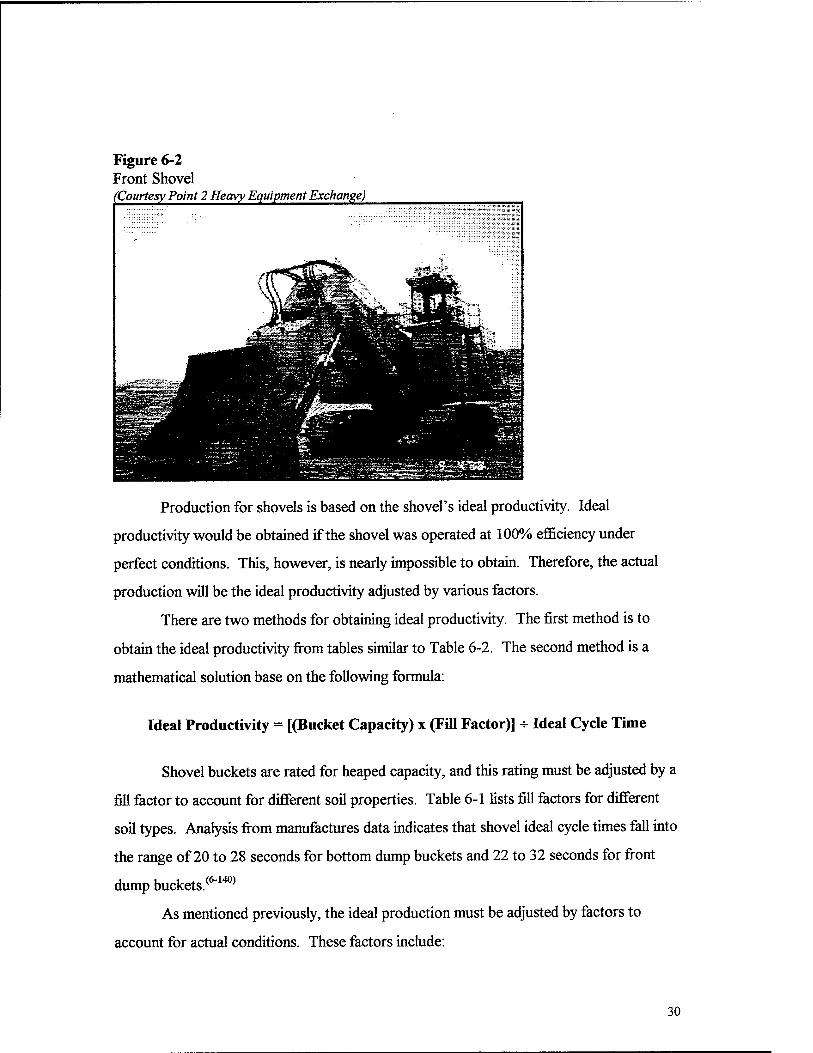
Figure 6-2 Front Shovel (Courtesy Point 2 Heavy Equipment Exchange)

Production for shovels is based on the shovel's ideal productivity. Ideal

productivity would be obtained if the shovel was operated at 100% efficiency under

perfect conditions. This, however, is nearly impossible to obtain. Therefore, the actual

production will be the ideal productivity adjusted by various factors.

There are two methods for obtaining ideal productivity. The first method is to

obtain the ideal productivity from tables similar to Table 6-2. The second method is a

mathematical solution base on the following formula:

Ideal Productivity = [(Bucket Capacity) x (Fill Factor)] ■*■ Ideal Cycle Time

Shovel buckets are rated for heaped capacity, and this rating must be adjusted by a

fill factor to account for different soil properties. Table 6-1 lists fill factors for different

soil types. Analysis from manufactures data indicates that shovel ideal cycle times fall into

the range of 20 to 28 seconds for bottom dump buckets and 22 to 32 seconds for front

dump buckets.(6"140)

As mentioned previously, the ideal production must be adjusted by factors to

account for actual conditions. These factors include:

30

• Swing/depth Factor (Table 6-3) • Efficiency Factor (Table 5-1)

and the actual productivity is given by:

Actual Productivity = Ideal Productivity x Efficiency Factor x Swing/depth Factor

Table 6-1 Bucket Fill Factors For Shovels Material Bucket Fill Factor Bank Clay; earth Rock/Earth Mixtures Poorly Blasted Rock Well Blasted Rock Shale; sandstone

1.00-1.10 1.05-1.15 0.85-1.00 1.00-1.10 0.85-1.10


Table 6-2 Ideal Shovel Productivity in Bank Cubic Yards per Hour (BCY/hr)

Bucket Capacity '/icy %cy 1 cy 1 lAcy 1*4 cy 1 % cy 2cy 2'/2cy Material

Moist Loam 115 165 205 250 285 320 355 405 Sand and Gravel 110 155 200 230 270 300 330 390 Common Earth 95 135 175 210 240 270 300 350 Tough Clay 75 110 145 180 210 235 265 310 Well blasted rock 60 95 125 155 180 205 230 275 Earth/rock mixture 50 80 105 130 155 180 200 245 Wet Clay 40 70 95 120 145 165 185 230 Poorly blasted rock 25 50 75 95 115 140 160 195


Table 6-3 Shovel Productivity Correction Factors for Depth of Cut and Angle of Swing % of Optimum

Depth Angle of

Swing 45° 60° 75° 90° 120° 150°


180° 40% 0.93 0.89 0.85 0.80 0.72 0.65 0.59 60% 1.10 1.03 0.96 0.91 0.81 0.73 0.66 80% 1.22 1.12 1.04 0.98 0.86 0.77 0.69 100% 1.26 1.16 1.07 1.00 0.88 0.79 0.71 120% 1.20 1.11 1.03 0.97 0.86 0.77 0.70 140% 1.12 1.04 0.97 0.91 0.81 0.73 0.66 160% 1.03 0.96 0.90 0.85 0.75 0.67 0.62

Example 6-1 A contractor elects to use a bottom dump front excavator with a 1 cubic yard

bucket and a 10 feet ideal depth of cut to perform the excavation for a new motel. The average depth of cut for this excavation will be 6 feet. The excavated material is common earth. The job conditions are excellent, while management conditions are fair. The job site provides for a 90 ° angle of swing, (a) Calculate the actual production of this shovel in BCY's based on an ideal productivity from table 6-2. (b) Calculate the actual production of this shovel in BCY's based on the ideal productivity formula. Solution

(a) Step 1 - Obtain Ideal Productivity (Table 6-2)

With 1 cy bucket and material common earth Ideal Productivity = 175 BCY/hr

Step 2 - Determine Efficiency Factor (Table 5-1) With Fair Management and Excellent Job Conditions

Efficiency Factor = 0.76 Step 3 - Determine Swing/Depth Factor (Table 6-3)

With 90 ° Angle of Swing and 60% depth of cut (6 VI0') Swing/Depth Factor = 0.91

Step 4 - Calculate Actual Production Actual Production = Ideal Production x Efficiency Factor x Swing/Depth Factor

Actual Production = 175 BCY/hr x 0.76x0.91 = 121.03BCY/hr (b) Step 1 - Obtain Ideal Productivity by Formula With: Bucket Fill Factor = 1.10 (Table 6-1)

Swell = 25% (Table 4-1) Ideal Cycle Time = 20 sec (estimated)

Ideal Productivity = [(Bucket Capacity) x (Fill Factor)] s- Ideal Cycle Time Ideal Productivity = [1 LCYx 1.10 x 3600 sec/hr] +[20 sec x 1.25 BCY/LCY]

Ideal Productivity = 158.4 BCY/hr Step 2 - Calculate Actual Production

Actual Production = 158.4 BCY/hr x0.76x 0.91 = 109.5 BCY/hr

Example 6-1 illustrates that different methods may produce slightly different

answers. It should also be noted that most manufactures have there own tables of

adjustment factors, and the factors will generally differ slightly between manufactures.

6.2. Backhoes

Another popular piece of equipment for excavating is the hydraulic backhoe,

Figure 6-3. Backhoes can be either wheel mounted or track mounted. Often small

wheeled tractors will have a small backhoe attachment, Figure 6-4. For larger excavations

32

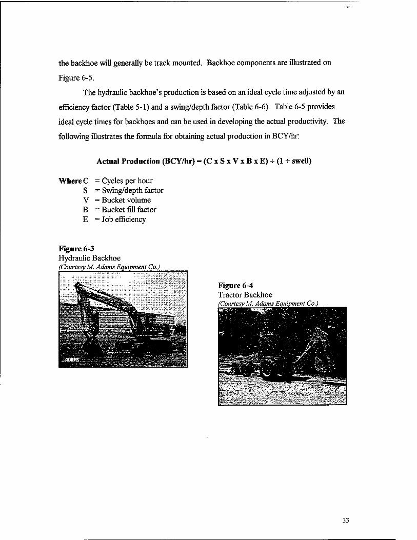
the backhoe will generally be track mounted. Backhoe components are illustrated on

Figure 6-5.

The hydraulic backhoe's production is based on an ideal cycle time adjusted by an

efficiency factor (Table 5-1) and a swing/depth factor (Table 6-6). Table 6-5 provides

ideal cycle times for backhoes and can be used in developing the actual productivity. The

following illustrates the formula for obtaining actual production in BCY/hr:

Actual Production (BCY/hr) = (CxSxVxBxE)^(l + swell)

c = Cycles per hour s = Swing/depth factor V = Bucket volume B = Bucket fill factor E = Job efficiency

Figure 6-3 Hydraulic Backhoe 'Courtesy M. Adams Equipment Co.)

Figure 6-4 Tractor Backhoe (Courtesy M. Adams Et went Co.)

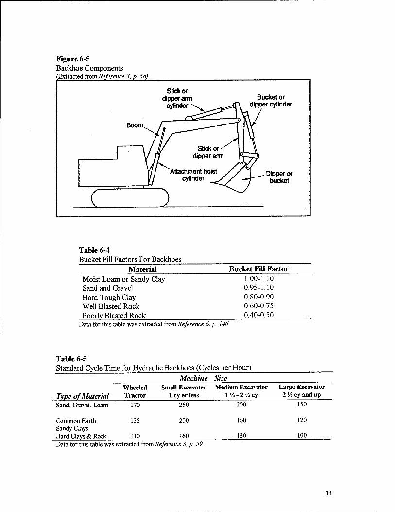
Figure 6-5 Backhoe Components (Extracted from Reference 3, p. 58)

Stick or dipper arm

cylinder

Boom

c

Bucket or dipper cylinder

Dipper or bucket

Table 6-4 Bucket Fill Factors For Backhoes

Material Bucket Fill Factor Moist Loam or Sandy Clay Sand and Gravel Hard Tough Clay Well Blasted Rock Poorly Blasted Rock

1.00-1.10 0.95-1.10 0.80-0.90 0.60-0.75 0.40-0.50


Table 6-5 Standard Cycle Time for Hydraulic Backhoes (Cycles per Hour)

Machine Size

Type of Material Wheeled Tractor

Small Excavator 1 cy or less

Medium Excavator 1 % - 2 V* cy

Large IVz

: Excavator cy and up

Sand, Gravel, Loam

Common Earth, Sandy Clays Hard Clays & Rock

170

135

110

250

200

160

200

160

130

150

120

100 Data for this table was extracted from Reference 3, p. 59

34

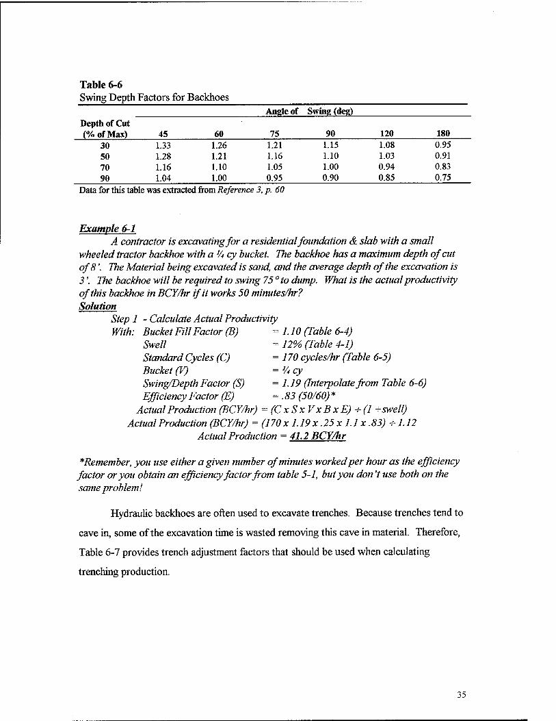
Table 6-6 Swing Depth Factors for Backhoes

Angle of Swing (deg) Depth of Cut (%ofMax) 45 60 75 90 120 180

30 1.33 1.26 1.21 1.15 1.08 0.95 50 1.28 1.21 1.16 1.10 1.03 0.91 70 1.16 1.10 1.05 1.00 0.94 0.83 90 1.04 1.00 0.95 0.90 0.85 0.75


Example 6-1 A contractor is excavating for a residential foundation & slab with a small

wheeled tractor backhoe with a 'A cy bucket. The backhoe has a maximum depth of cut of 8'. The Material being excavated is sand, and the average depth of the excavation is 3'. The backhoe will be required to swing 75 ° to dump. What is the actual productivity of this backhoe in BCY/hr if it works 50 minutes/hr? Solution

Step 1 - Calculate Actual Productivity With: Bucket Fill Factor (B) = 1.10 (Table 6-4)

Swell = 12% (Table 4-1) Standard Cycles (C) =170 cycles/hr (Table 6-5) Bucket (V) = 'Acy Swing/Depth Factor (S) = 1.19 (Interpolate from Table 6-6) Efficiency Factor (E) = .83 (50/60) *

Actual Production (BCY/hr) = (CxSxVxBxE) -i-(l +swell) Actual Production (BCY/hr) = (170 x 1.19 x .25 x 1.1 x .83) s-1.12

Actual Production = 41.2 BCY/hr

*Remember, you use either a given number of minutes worked per hour as the efficiency factor or you obtain an efficiency factor from table 5-1, but you don't use both on the same problem!

Hydraulic backhoes are often used to excavate trenches. Because trenches tend to

cave in, some of the excavation time is wasted removing this cave in material. Therefore,

Table 6-7 provides trench adjustment factors that should be used when calculating

trenching production.

35

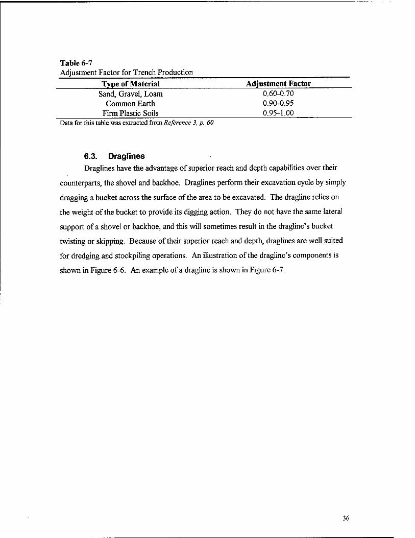
Table 6-7 Adjustment Factor for Trench Production Type of Material Adjustment Factor

Sand, Gravel, Loam 0.60-0.70 Common Earth 0.90-0.95

Firm Plastic Soils 0.95-1.00 Data for this table was extracted from Reference 3, p. 60

6.3. Draglines Draglines have the advantage of superior reach and depth capabilities over their

counterparts, the shovel and backhoe. Draglines perform their excavation cycle by simply

dragging a bucket across the surface of the area to be excavated. The dragline relies on

the weight of the bucket to provide its digging action. They do not have the same lateral

support of a shovel or backhoe, and this will sometimes result in the dragline's bucket

twisting or skipping. Because of their superior reach and depth, draglines are well suited

for dredging and stockpiling operations. An illustration of the dragline's components is

shown in Figure 6-6. An example of a dragline is shown in Figure 6-7.

36

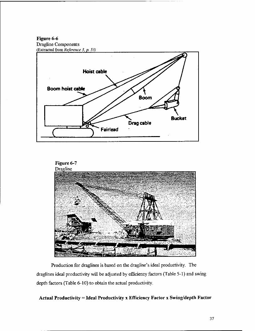
Figure 6-6 Dragline Components (Extracted from Reference 3, p. 53)

Hoist cable

Boom hoist cable

I Bucket

Figure 6-7 Dragline

äaaa^lis&s&siSd.

Production for draglines is based on the dragline's ideal productivity. The

draglines ideal productivity will be adjusted by efficiency factors (Table 5-1) and swing

depth factors (Table 6-10) to obtain the actual productivity.

Actual Productivity = Ideal Productivity x Efficiency Factor x Swing/depth Factor

37

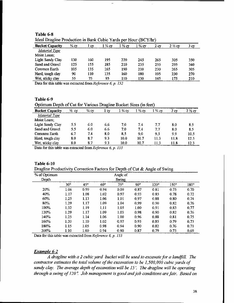
Table 6-8 Ideal Dragline Production in Bank Cubic Yards per Hour (BCY/hr) Bucket Capacity %cy 1 cy 1 Vicy 1 Vicy l3/4cy 2cy IVzcy 3cy

Material Tvpe Moist Loam; Light Sandy Clay 130 160 195 220 245 265 305 350 Sand and Gravel 125 155 185 210 235 255 295 340 Common Earth 105 135 165 190 210 230 265 305 Hard, tough clay 90 110 135 160 180 195 230 270 Wet, sticky clay 55 75 95 110 130 145 175 210 Data for this table was extracted from Reference 6, p. 152

Table 6-9 Optimum Depth of Cut for Various Dragline Bucket Sizes (in feet) Bucket Capacity Vi cy 3/4cy 1 cy IVicy 1 Vicy l3/4cy 2cy 2 Vicy

Material Tvpe Moist Loam; Light Sandy Clay 5.5 6.0 6.6 7.0 7.4 7.7 8.0 8.5 Sand and Gravel 5.5 6.0 6.6 7.0 7.4 7.7 8.0 8.5 Common Earth 6.7 7.4 8.0 8.5 9.0 9.5 9.9 10.5 Hard, tough clay 8.0 8.7 9.3 10.0 10.7 11.3 11.8 12.3 Wet, sticky clay 8.0 8.7 9.3 10.0 10.7 11.3 11.8 12.3 Data for this table was extracted from Reference 6, p. 153

Table 6-10 Dragline Productivity Correction Factors for Depth of Cut & Angle of Swing % of Optimum Angle of

Depth Swing 30° 45° 60° 75° 90° 120° 150° 180°

20% 1.06 0.99 0.94 0.09 0.87 0.81 0.75 0.70 40% 1.17 1.08 1.02 0.97 0.93 0.85 0.78 0.72 60% 1.25 1.13 1.06 1.01 0.97 0.88 0.80 0.74 80% 1.29 1.17 1.09 1.04 0.99 0.90 0.82 0.76 100% 1.32 1.19 1.11 1.05 1.00 0.91 0.83 0.77 120% 1.29 1.17 1.09 1.03 0.98 0.90 0.82 0.76 140% 1.25 1.14 1.06 1.00 0.96 0.88 0.81 0.75 160% 1.20 1.10 1.02 0.97 0.93 0.85 0.79 0.73 180% 1.15 1.05 0.98 0.94 0.90 0.82 0.76 0.71 200% 1.10 1.00 0.94 0.90 0.87 0.79 0.73 0.69


Example 6-2 A dragline with a 2 cubic yard bucket will be used to excavate for a landfill. The

contractor estimates the total volume of the excavation to be 1,500,000 cubic yards of sandy clay. The average depth of excavation will be 15'. The dragline will be operating through a swing of 120 °. Job management is good arid job conditions are fair. Based on

38

this information what will the actual production be in bank cubic yards per hour (BCY/hr)? Additionally, what will the expected duration be for this excavation? Solution

Step 1 - Calculate Ideal Production Ideal Production = 265 BCY/hr (Table 6-8)

Step 2 - Calculate Swing/depth Factor Optimum depth of cut = 8.0' (Table 6-9) % of Optimum = 15 V8 'xlOO = 187.5%

Swing = 120° Swing/depth Factor = 0.81 (Table 6-10)

Step 3 - Calculate Efficiency Factor Efficiency Factor = 0.69 (Table 5-1)

Step 4 - Calculate Actual Production Actual Productivity = Ideal Productivity x Efficiency Factor x Swing/depth Factor

Actual Productivity = 265BCY/hrx 0.69x0.81 Actual Productivity = 148.1 BCY/hr

Step 5 - Calculate Duration Duration = Quantity of Excavation -v- Actual Production

Duration = 1,500,000 -#-148.1 BCY/hr Duration = 10.128.3 hrs. or 422 days

39

7. Tractors/Dozers Tractors/dozers are a common sight on most construction sites. They are of two

variants, either wheel type (Figure 7-1) or track type (Figure 7-2). Some common uses of

tractors/dozers include:

• Backfilling • Clearing & grubbing • Creating stockpiles • Excavating • Slope shaping • Spreading materials • Towing • Rough grading

There are many ways to calculate tractor/dozer production. Some methods

include calculating theoretical blade capacity coupled with equipment cycle time and other

factors. However, equipment manufactures generally have production charts, similar to

Figure 7-3, for aiding the equipment manager in estimating production. These production

estimating charts combined with the correction factors provided in Table 7-1 will provide

the basis for evaluating tractor/dozer production here.

Figure 7-1 Wheel Type Dozer (Courtesy Caterpillar)

Figure 7-2 Track Type Dozer (Courtesy M. Adams EauipmentCo.)

40

Figure 7-3 Estimated Dozing Production (Extracted from Reference 1, p. 113)

Lnfilw LCY/hr 011IMI

2400

2200

2000

1800

1600

1400

1200

1000

800

600

400

200

3000

2800

-2600

_2400

2200

2000

-1800

_1600

1400

1200

"1000

-800

600

400

" 200

(W »Ml 1

h JMJ\

DWM

0704 \\

.—PIUMI

LOMHI 1 4

if ■«• •• i^- "^"«■1 1 OTH4J 1 i u u

I 1(

L .. 1 10 20

1 1 10 300 400 500 600

l l 1 1 1 1 1 t 1 FEET

I

0 15 30 45 60 75 00 105 120 135 150165 160 1«

AVERAGE OOZING DISTANCE

i METERS

41

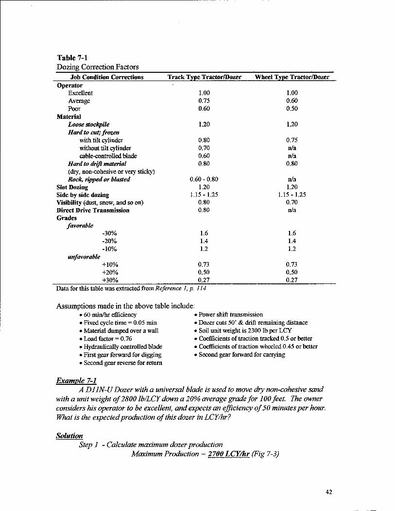
Table 7-1 Dozing Correction Factors

Job Condition Corrections Track Type Tractor/Dozer Wheel Type Tractor/Dozer

1.00 0.60 0.50

1.20

0.75 n/a n/a

0.80

n/a 1.20

1.15 - 1.25 0.70 n/a

1.6 1.4 1.2

0.73 0.50 027 Data for this table was extracted from Reference 1, p. 114

Assumptions made in the above table include: • 60 min/hr efficiency • Power shift transmission • Fixed cycle time = 0.05 min • Dozer cuts 50' & drift remaining distance • Material dumped over a wall • Soil unit weight is 2300 lb per LCY • Load factor = 0.76 • Coefficients of traction tracked 0.5 or better • Hydraulically controlled blade • Coefficients of traction wheeled 0.45 or better • First gear forward for digging • Second gear forward for carrying • Second gear reverse for return

Example 7-1 A D11N-U Dozer with a universal blade is used to move dry non-cohesive sand

with a unit weight of 2800 lb/LCY down a 20% average grade for 100 feet. The owner considers his operator to be excellent, and expects an efficiency of 50 minutes per hour. What is the expected production of this dozer in LCY/hr?

Operator Excellent 1.00 Average 0.75 Poor 0.60

Material Loose stockpile 1.20 Hard to cut; frozen

with tilt cylinder 0.80 without tilt cylinder 0.70 cable-controlled blade 0.60

Hard to drift material 0.80 (dry, non-cohesive or very sticky) Rock, ripped or blasted 0.60 - 0.80

Slot Dozing 1.20 Side by side dozing 1.15 - 1.25 Visibility (dust, snow, and so on) 0.80 Direct Drive Transmission 0.80 Grades

favorable -30% 1.6 -20% 1.4 -10% 1.2

unfavorable +10% 0.73 +20% 0.50 +30% 0.27

Solution Step 1 - Calculate maximum dozer production

Maximum Production = 2700 LCY/hr (Fig 7-3)

42

Step 2 - Determine applicable correction factors (Table 7-1) Excellent operator = 1.00 Non-cohesive sand = 0.80 Grade of-20% =1.40 Weight correction = 0.82 (2300/2800, see assumptions for Table 7-1) Efficiency = 0.83 Step 3 - Calculate expected production

Expected Production = Maximum Production x Correction Factors Expected Production = 2700 xl.OOx 0.80 x 1.40 x 0.82 x 0.83

Expected Production = 2058.1 LCY/hr

43

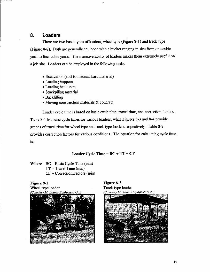
8. Loaders There are two basic types of loaders; wheel type (Figure 8-1) and track type

(Figure 8-2). Both are generally equipped with a bucket ranging in size from one cubic

yard to four cubic yards. The maneuverability of loaders makes them extremely useful on

a job site. Loaders can be employed in the following tasks:

• Excavation (soft to medium hard material) • Loading hoppers • Loading haul units • Stockpiling material • Backfilling • Moving construction materials & concrete

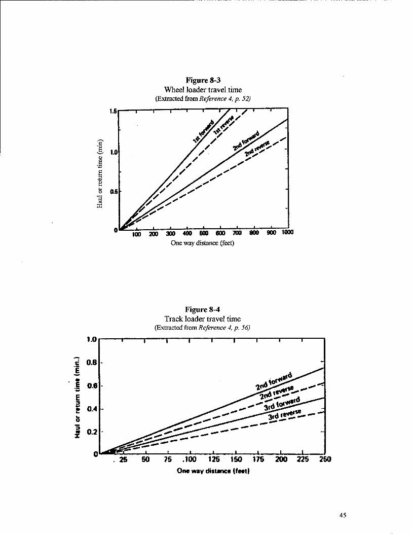
Loader cycle time is based on basic cycle time, travel time, and correction factors.

Table 8-1 list basic cycle times for various loaders, while Figures 8-3 and 8-4 provide

graphs of travel time for wheel type and track type loaders respectively. Table 8-2

provides correction factors for various conditions. The equation for calculating cycle time

is:

Loader Cycle Time = BC + TT + CF

Where BC = Basic Cycle Time (min) TT = Travel Time (min) CF = Correction Factors (min)

Figure 8-1 Wheel type loader (Courtesy M. Adams Equipment Co.)

BOSS?

;ffJK^^j^j: ,^?ZL*%\_** *7iT,,~fr?*X''l -^JtZtl **?■-£ - ^ ^■'-'^ ^■L~JS£*T'5**r:z~$iJ

Figure 8-2 Track type loader (Courtesy M. Adams Equipment Co.)

44

I 1 e s

3 es

Figure 8-3 Wheel loader travel time

(Extracted from Reference 4, p. 52)

100 200300400600600700800900 1000

One way distance (feet)

Figure 8-4 Track loader travel time

(Extracted from Reference 4, p. 56)

250 One way distance (feet)

45

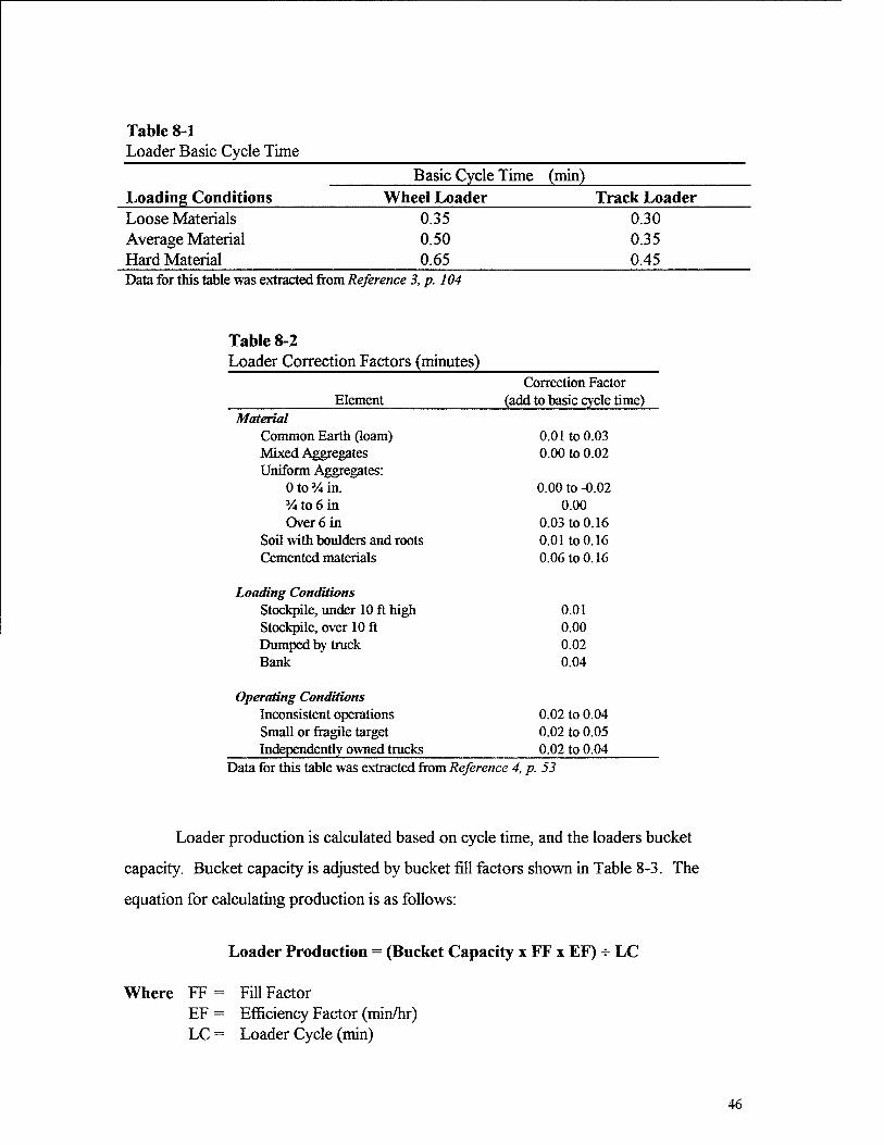
Table 8-1 Loader Basic Cycle Time

Basic Cycle Time (min) Loading Conditions Wheel Loader Track Loader Loose Materials Average Material Hard Material

0.35 0.30 0.50 0.35 0.65 0.45


Table 8-2 Loader Correction Factors (minutes)

Correction Factor Element (add to basic cycle time)

Material Common Earth (loam) 0.01 to 0.03 Mixed Aggregates 0.00 to 0.02 Uniform Aggregates:

0 to J/4 in. 0.00 to -0.02 % to 6 in 0.00 Over 6 in 0.03 to 0.16

Soil with boulders and roots 0.01 to 0.16 Cemented materials 0.06 to 0.16

Loading Conditions Stockpile, under 10 ft high 0.01 Stockpile, over 10 ft 0.00 Dumped by truck 0.02 Bank 0.04

Operating Conditions Inconsistent operations 0.02 to 0.04 Small or fragile target 0.02 to 0.05 Independently owned trucks 0.02 to 0.04


Loader production is calculated based on cycle time, and the loaders bucket

capacity. Bucket capacity is adjusted by bucket fill factors shown in Table 8-3. The

equation for calculating production is as follows:

Loader Production = (Bucket Capacity x FF x EF) ^ LC

Where FF = Fill Factor EF = Efficiency Factor (min/hr) LC = Loader Cycle (min)

46

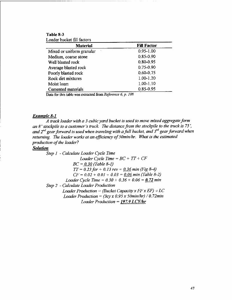
Table 8-3 Loader bucket fill factors Material Fill Factor Mixed or uniform granular 0.95-1.00 Medium, coarse stone 0.85-0.90 Well blasted rock 0.80-0.95 Average blasted rock 0.75-0.90 Poorly blasted rock 0.60-0.75 Rock dirt mixtures 1.00-1.20 Moist loam 1.00-1.10 Cemented materials 0.85-0.95


Example 8-1 A track loader with a 3 cubic yard bucket is used to move mixed aggregate form

an 8' stockpile to a customer's truck. The distance from the stockpile to the truck is 75', and 2nd gear forward is used when traveling with a full bucket, and 3rd gear forward when returning. The loader works at an efficiency ofSOmin/hr. What is the estimated production of the loader? Solution

Step 1 - Calculate Loader Cycle Time Loader Cycle Time =BC+TT+CF

BC = 0.30 (Table 8-1) TT = 0.23 for + 0.13 rev = 0J6 min (Fig 8-4) CF =0.02 + 0.01 + 0.03 = 0M min (Table 8-2)

Loader Cycle Time = 0.30 + 0.36 +0.06 = 0J2 min Step 2 - Calculate Loader Production

Loader Production = (Bucket Capacity x FF x EF) +LC Loader Production = (3cy x0.95x 50min/hr) / 0.72min

Loader Production = 197.9 LCY/hr

47

9. Hauling Equipment In estimating hauling equipment cycle times and production it is import to consider

some additional factors. These factors include the equipment's rolling resistance, grade

resistance, and effective grade. The total resistance of a piece of equipment will be:

Total Resistance = Rolling Resistance + Grade Resistance

Resistance is typically expressed in pounds per ton of vehicle weight (lb/ton) or in pounds

(lb's) only. For the purposes of this report, resistance factors will carry the unit of lb/ton

and resistance will cany the unit of lb's.

9.1. Rolling Resistance Rolling resistance is primarily a factor of the resistance incurred from tire flexing

and penetration of tires into the surface being traversed. It has been shown that a vehicle

traveling over a hard surface roadway will have a rolling resistance factor of about 40

lb/ton of vehicle weight, and this will increase by 30 lb/ton of vehicle weight for each inch

of tire surface penetration. This leads to the following equation for rolling resistance

factor:

Rolling Resistance Factor (lb/ton) = 40 + (30 x Inches of tire penetration)

Table 9-1 provides a list of some typical values of rolling resistance factors.

Table 9-1 Typical Values of Rolling Resistance Factors Type of Surface Rolling Resistance Factor (lb/ton) Concrete or Asphalt 40 (30)* Firm, smooth, flexing slightly under load 64 (52)* Rutted dirt roadway, 1-2 inches penetration 100 Soft, rutted dirt, 3-4 inches penetration 150 Loose sand or gravel 200 Soft, muddy, deeply rutted 300-400 * Values in parenthesis are for radial tires Data for this table was extracted from Reference 3, p. 84

48

9.2. Grade Resistance

Grade resistance results from resistance encountered as a result of positive or

negative grades. Grade resistance is that component of resistance acting parallel to the

grade. The actual grade resistance can be obtained by multiplying the sine of the angle of

grade with respect to horizontal by the vehicles weight. However, because the grades in

construction are typically small, it is generally accepted that 1% of grade will have a grade

resistance of 1% of a vehicles weight. This corresponds to a grade resistance factor of

201b/ton for each 1% of grade, or:

Grade Resistance Factor (lb/ton) = 20 x grade (%) Grade Resistance (lb) = Vehicle wight (tons) x Grade Resistance Factor (lb/ton)

9.3. Effective Grade Effective grade is a simple method of representing the sum of rolling resistance and

grade resistance. Effective grade is important because it is often used in equipment

manufactures performance charts for estimating equipment performance parameters.

Effective grade is the method that will be demonstrated in this paper. The equation for

effective grade is given by:

Effective Grade = Grade (%) + [Rolling Resistance Factor (lb/ton) -s- 20]

9.4. Scrapers A scraper is a single piece of equipment that has the ability to excavate, load, haul,

and dump. There are a number of different scraper types including:

• Single Engine Overhung • Three Axle • Twin Engine, All Wheel Drive (Figure 9-1) • Elevating (Figure 9-2) • Push Pull

49

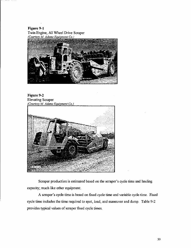
Figure 9-1 Twin Engine, All Wheel Drive Scraper

Figure 9-2 Elevating Scraper (Courtesy M. Adams Equipment Co.)

Ä

Scraper production is estimated based on the scraper's cycle time and hauling

capacity; much like other equipment.

A scraper's cycle time is based on fixed cycle time and variable cycle time. Fixed

cycle time includes the time required to spot, load, and maneuver and dump. Table 9-2

provides typical values of scraper fixed cycle times.

50

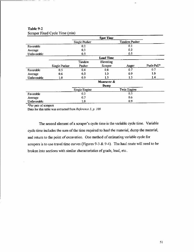
Table 9-2 Scraper Fixed Cycle Time (min)

Spot Time Single Pusher Tandem Pusher

Favorable Average Unfavorable

0.2 0.3 0.5

0.1 0.2 0.5

Load Time

Single Pusher Tandem Pusher

Elevating Scraper Auger Push-Pull*

Favorable Average Unfavorable

0.5 0.6 1.0

0.4 0.5 0.9

0.8 1.0 1.5

0.7 0.9 1.3

0.7 1.0 1.4

Maneuver & Dump

Single Engine Twin Engine Favorable Average Unfavorable

0.3 0.7 1.0

0.3 0.6 0.9

*Per pair of scrapers Data for this table was extracted from Reference 3, p. 109

The second element of a scraper's cycle time is the variable cycle time. Variable

cycle time includes the sum of the time required to haul the material, dump the material,

and return to the point of excavation. One method of estimating variable cycle for

scrapers is to use travel time curves (Figures 9-3 & 9-4). The haul route will need to be

broken into sections with similar characteristics of grade, load, etc..

51

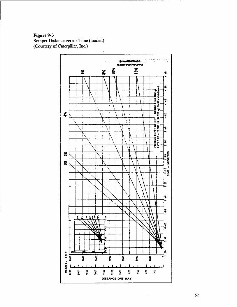
Figure 9-3 Scraper Distance versus Time (loaded) (Courtesy of Caterpillar, Inc.)

\ \ \

E is— «• >• <J m _ «V

M —

8 o s- m

§ 1

O < — o >

o

'*■

o «■

'V

o

«

o

"•*

•V»

'-§

a *■ UJ

o o M

O

O W

O

O

0

o

o o

\ i

j \ \ . i * K ! \

I \ M

8

: : i V ! \ ;\i ! ; ,; ! ! ■ : N ■ ' V \ - V 1 i

£ N - ■ : \j I 1 i\ : ■ » ! ? \ . . K j !\\: ■ I IS •\! ■ ■ \i : \! \l . it s ■ \: : : K i \ !\ i !\

m. 2 IM

i i i \ \j \ I\ >

\ ! I\l \ \ *

v i \ ! ] f\ ! \ \

Si V! 1 i N , j \ \ A \ * V

\ \

\\ i v \

\ \ \ \ \ v>

V \ ^

A \ \ \

\ v \\ \

V \ N A ,\

V \ \>

\

i t f '.a'-. 5 IN h" s\ \\ NN: \\\

v ^

^ ^ s m \ f-

^ ^8 \ * — Ti u

«- m> F ■ »•■ -T^

M

§ i 1 p* 9> SS

t . i . i . i . i . i . i , 1 .

i i i . i . i . i

»**

*- *i

8 i 1 § 5 g 1 § 1 § 2 DISTANCE ONE WAV

52

Figure 9-4 Scraper Distance versus Time (empty) (Courtesy of Caterpillar, Inc.)

TOTAL MBCTJVCf g * WUOCfUftMUMO

o «M

\ s

0

\ 1 w - o

m * >-

\ \ ! i i • \ • . 1

y !\i : ! : \ ■ i :

: N ! \ i ■ ; \ : ! ! i 1 1°

1 \ IM -1 u

" X w >

«9 w*

eM • U*

'-S z i

5 i

s

o «9

o »

o

o «• o

a

~o

o o

\ 1 \ ! : i\ i i \ ; i ' \ \ 1 1 ' \ 1

1 \ 1 \

I \

^ \ \

\

\ \ •v \

\ \ 1 \

\s \ > \ \ \

i Hi i s ^ ^ V\ ^ \ 1

v^ ^

• s ̂ ssi\

1 \ t a v- s

Ml Ml

«• «M

Mi— §

1 . 1 . 1 . 1 . 1 . 1 . 1 . 1 . 1 . 1 . 1 . 1

I 1 i I § 1 § § I § 1 2 DISTANCE OWE WAY

53

In determining a scrapers per cycle capacity, one must consider both the scrapers

rated payload capacity and volumetric capacity. The governing value will be the lesser of

the two capacities. For example, if a scraper is rated for a 50,000 lb payload and 30

LCY's volume, and the material being excavate has a unit weight of 2,000 lb/LCY, then

payload would govern, because 30 LCY's of a 2,000 lb/LCY material would weigh

60,000 lb, which exceeds the rated payload capacity. Therefore, in this example the

scraper could only handle a volume of 50,000 lb divided by 2,000 lb/LCY or 25 LCY of

material not the rated 30 LCY.

Example 9-1 A single engine tandem pusher scraper, which has travel time/distance curves as

shown in figures 9-3 & 9-4 is being used to excavate for a large parking lot. The scraper has a heaped volume capacity of 30 LCY, and a maximum payload capacity of 65,000 lb. The material being removed is sand with a unit weight of 2,800 lb/LCY and 3,200 lb/BCY. The job conditions are average and job efficiency is equivalent to 50 min/hr. The scraper is working in a dirt roadway environment with approximately 1.5 inch of tire penetration. The haul route can be broken up as follows:

1. Level loading area 2. Haul down a 4% grade for 1,500 feet 3. Level dump area 4. Return up a 4% grade for 1,500 feet 5. Level turnaround of 600 feet

Based on this information, what will is the estimated scraper production? Solution

Step 1- Calculate weight of heaped capacity Weight of Heaped Capacity = Loose Unit Weight x Capacity = 2,800 lb/LCY x 30 LCY

Weight of Heaped Capacity = 84,000 lb Note: Weight of heaped capacity (84,000 lb) exceeds rated payload capacity of 65,000 lb, therefore scraper will work at less than heaped capacity. Step 2 - Calculate Maximum Capacity (BCY)

Maximum Capacity (BCY) = Payload Capacity + Bank Unit Weight Maximum Capacity (BCY) = 65,000 lb + 3,200 lb/BCY

Maximum Capacity = 20.31 BCY Step 3 - Calculate Effective Grades (EG) Where:

EG = Grade (%) + [Rolling Resistance Factor (lb/ton) +20] Haul:

EG = -4% + [100 +20] = 1% Return:

EG = 4% + [100+20] = 9%

54

Turnaround: EG = 0% + [100 +20] = 5%

Step 4 - Calculate variable cycle time from Figures 9-3 & 9-4 Haul =0.84 min Return = 1.20 min Turnaround = 0.41 min

Step 5 - Calculate fixed cycle time from Table 9-2 Spot = 0.2 min Load =0.5 min Maneuver/Dump = 0.7 min

Step 6 - Calculate Total Cycle Time Total Cycle = fixedcycle + variable = 0.84 + 1.20 + 0.41 + 0.2 + 0.5 + 0.7

Total Cycle = 3.85 min Step 7 - Calculate estimated production

Estimated Production = [Maximum Capacity (BCY) x Efficiency (min/hr)] + Total Cycle Estimated Production = [20.31 BCYx 50 min/hr] + 3.85 min

Estimated Production = 263.8 BCY/hr

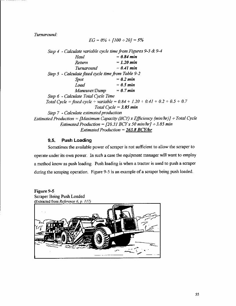
9.5. Push Loading Sometimes the available power of scraper is not sufficient to allow the scraper to

operate under its own power. In such a case the equipment manager will want to employ

a method know as push loading. Push loading is when a tractor is used to push a scraper

during the scraping operation. Figure 9-5 is an example of a scraper being push loaded.

Figure 9-5 Scraper Being Push Loaded (Extracted from Reference 6, p. 117)

55

There are three basic methods of push loading. The three methods are Back Track

Loading, Chain Loading, and Shuttle Loading. Figure 9-6 illustrates the three methods of

push loading. Typically push loading will be accomplished by using either one pusher per

scraper or two pushers per scraper.

56

Figure 9-6 Methods of Push Loading (Extracted from Reference 3, p. 113)

, Scraper,

Loading Loaded

Pusher tractor

Fsna—&*2nfi^r-^ -ffl K*3"^ SS_JteLTcJLv> N "S S=n-rd

--SÜZS30 Back-track loading

sms^'N loses Chain loading & K~S1 w*

CTT aazsra^-r- npr

cc irfL

i i x/ Shuttle ^ I, ' loading

57

Because a tractor is involved in a push loading operation, it is important to be able

to determine the number of scrapers that a pusher can support, and the number of pushers

required to support a fleet of scrapers. These numbers can be obtained with the following

equations:

No. scrapers served by one pusher = Scraper Cycle Time -^Pusher Cycle Time

Number of Pushers Required = Number of Scrapers 4- No. scrapers served by one

pusher

Table 9-3 provides a list of typical pusher cycle times.

Table 9-3 Typical Pusher Cycle Times (min)

Loading Method Single Pusher Tandem Pusher Back Track Chain or Shuttle

1.5 1.0

1.4 0.9


To determine the expected production of a scraper fleet the following equation

applies:

Fleet Production = [No. of Pushers -s- No. Pushers Required] x No. Scrapers x Single Scraper Production

Example 9-2 A contractor is employing a fleet of 6 scrapers with single pushers for back track

push loading. The estimated cycle time for each scraper is 5 minutes. The scrapers have a capacity of 200 BCYper hour, and the contractor has 3 dozers available for pushig. (a) What is the number of pushers required to serve the fleet? (b) What is the estimated production of this fleet? Solution

(a) No. scrapers served by one pusher = 5 min +1.5 = 3.33 scrapers/pusher

No. pushers required =6+3.33 = 1.8 use 2 pushers (b)

Fleet Production = [3 -r-3.33] x 6x 200 BCY/hr = 1081.1 BCY/hr

58

9.6. Trucks It is obvious that hauling is a major part of any earthmoving process, and the most

prevalent piece of equipment used for hauling materials in the construction industry is the

truck. Many trucks are licensed for highway use, which is of particular usefulness when a

borrow pit or dump site is located some distance from the construction site. Knowing that

trucks are one of the most popular haulers, it is important to be familiar with estimating

truck production.

Truck production is based on cycle time. A truck's cycle time has two

components, fixed cycle time and variable cycle time. Fixed cycle time is the time required

for spot, maneuver, and dump. Table 9-4 list typical fixed cycle times for trucks. The

second component of truck cycle time is the variable component. Variable cycle time

consists of the load time and haul time. Load time is given by the following equation:

Load Time = Haul Unit Capacity + Loader Production

The haul time can simply be calculated by dividing the distance to the dump site by the

average speed of the truck.

Table 9-4 Typical Truck Fixed Cycle Times (min)

Bottom Dump Rear Dump Favorable 1.1 Average 1.6 Unfavorable 2.0

0.5 1.1 2.5


Because it is inefficient to have either loaders or haulers sitting idle, it is important

to accurately calculate the number of haul units required to support a loading operation.

The number of haulers required to support a loading operation is given by:

Number of haulers required = Haul Unit Cycle Time -^ Load Time

The aforementioned equation provides the theoretical number of haulers required

for a loading operation, however, the actual number of haulers available may differ from

59

the theoretical number required. When the actual number of haulers differs from the

theoretical number required, production can be estimated with the following equation:

Expected Production = (Haul Units Available 4- Number Haulers Required) x loader production

Example 9-3 Based on the following loader truck operation, (a) calculate the number of trucks

required theoretically to support the operation; (b) calculate the expected production if 8 trucks are available.

Loader Production = 350 BCY/hr Job Efficiency = 50 min/hr Truck Capacity = 20 BCY Truck Cycle Time = 0.5 hr (not including loading)

Solution (a) Step 1 - Calculate Load Time

Load Time = Haul Unit Capacity +Loader Production = 20 BCY + 350 BCY/hr Load Time = 0.057 hr

Step 2 - Calculate Truck Cycle Time Truck Cycle = 0.5 hr + 0.057 hr = 0.557hr

Step 3 - Calculate Number Trucks Required Number Trucks Required = Haul Unit Cycle Time -v-Load Time

Number Trucks Required = 0.557 hr + 0.057 Number Trucks Required = 9.8 (in theory)

0>) Step 1 - Calculate Expected Production of 8 Trucks

Expected Production = (Haul Units Available + Number Haulers Required) x loader production

Expected Production = (8+9.8)x 50min/60min x 350 BCY/hr Expected Production = 238 BCY/hr

60

10. Equipment Selection It is often necessary for an equipment manager to evaluate two equipment

alternatives to determine which is the most advantageous. The alternatives being

evaluated will likely have different costs per quantity, costs per time, and fixed costs.

There are several methods for making this determination, but only one method will be

presented here, and that method is the Line of Balance Method.

10.1. Line of Balance The Line of Balance Method is a mathematical model for analyzing two equipment

alternatives for the purpose of selecting the most advantageous.

To employ the Line of Balance Method a cost equation for each option must be

developed. The equation will take into account fixed costs, time dependant costs, and

quantity dependant costs.

Fixed Costs include, but are not limited to:

• Move In • Move Out • Mobilization • Demobilization • Purchase Price

Time dependant costs include, but are not limited to:

• Rental Costs • Interest

Quantity dependant costs include, but are not limited to:

• Wages • Operating Costs

The total costs of each option will include the sum of fixed costs, time dependant

costs, and quantity dependant costs. The following equation represents the total costs of a

given option:

Ct = Cf+Ctd + Cqty

61

Where Ct = Total Cost Cf = Fixed Costs Ctd = Time Dependant Costs Cqty = Quantity Dependant Costs

Example 10-1 Find the cost equation for an equipment option with the following cost data:

Move in/Move out =$2,000 Monthly Rental = $1,500/month Productivity = 6 CY/hr Labor Costs = $25/hr Operating Costs = $5/hr

Equation

Where

Ct = 2,000 + 1.500T + [($25 + $5)+6 CY/hr]Q Ct = 2,000 + 1,500T+5Q

T = Time (months) Q = Quantity (cubic yards)

Once the equation for each option is obtained, the equations are set equal to one

another, such that the resulting combined equation is that of a straight line. This equation

is then plotted. From this plot a determination of which option is best for a given quantity

and time can be made. The following example illustrates the entire Line of Balance

Method.

Example 10-2 Data

Small Mixer Large Mixer Mobilization/Demobilization $2,000 $4,000 Monthly Rental Costs $1,500/month $2,500/month Productivity 6CY/hr 10CY/hr Number of Laborers 5 3 Wages $5/hr $6/hr Operating Cost $5/hr $2/hr

This equipment will be used to place 1000 cubic yards of concrete, and it must be completed within 3 months. Which mixer is more advantageous? Solution

Step 1 -Calculate the cost equation for the small mixer Csmall mixer = 2,000 + 1,500T + [(($5 x 5)+ $5) + 6 CY/hrJQ

Csmall mixer = 2,000 + 1,500T+ SQ Step 2 - Calculate the cost equation for the large mixer

62

Clarge mixer = 4,000 + 2,500T + [(($6 x 3)+ $2)J +10 CY/hrJQ Clarge mixer = 4,000 + 2,500T+2Q

Step 3 - Combine Cost Equations Csmall mixer = Clarge mixer

2000 + 1.500T+ 5Q = 4,000 + 2,500T+ 2Q Q = (2,000+ 10001)+3

Step 4 - Plot combined equation

Combined Equation Plot

5000 -r

4 6 8

Time (months)

Step 5 - Use 3 months and 1,000 cubic yards and solve for each mixer equation. Small Mixer

Csmall mixer = 2,000 + 1,500(3) + 5(1000) Csmall mixer = $11,500

Large Mixer Clarge mixer = 4,000 + 2,500(3) + 2(1000)

Clarge mixer = $13,500

From this it can be determined that at 3 months and 1000 cubic yards the small mixer is more advantageous, and the intersection of 3 months and 1000 cubic yards falls below the plotted line. Therefore, the area below the line represents the area more advantageous to the small mixer and visa versa.

What would happen if there was a mistake in estimating the quantity, and the job required 2,000 cubic yards instead of 1,000 cubic yards?

63

In this case the intersection of 3 months and 2,000 cubic yards falls above the plotted line. Therefore, the large mixer would be selected.

In the preceding example the Line of Balance Method was used to evaluate two

pieces of equipment. It should be noted that this method is not limited to only two pieces

of equipment. This method could be used to analyze multiple options.

64

References

1. Day, David A., Construction Equipment Guide, Second Edition, John Wiley & Sons, Inc., New York, 1991

2. Drevdahl, Elmer R., Fundamentals of Excavation Equipment, Roadrunner Technical Publications Desert Laboratories, Inc., Arizona, 1963

3. Nunnally, S. W., Construction Methods and Management, Prentice-Hall, Inc., New Jersey, 1998

4. Nunnally, S. W., Managing Construction Equipment, Prentice-Hall, Inc., New Jersey, 1977

5. Peurifoy, R. L. and W. B. Ledbetter, Construction Planning Equipment, and Methods, Fourth Edition, McGraw-Hill, Inc., 1985

6. Schaufelberger, John E., Construction Eguipment Management, Prentice- Hall, Inc., New Jersey, 1999

7. White, John A, Marvin H. Agee, and Kenneth E. Case, Principles of Engineering Economic Analysis, Third Edition, John Wiley & Sons, Inc., New York, 1989

8. U. S. Army Corps of Engineers, Construction Equipment Ownership and Operating Expense Schedule, Volume II, August 1995

9. Rental Rate Blue Book, Volume 1, Dataquest Incorporated, 1992

65

Appendix A Compound Interest Tables

66

Compound Intereste Table for: i = 1%

Single Payment Uniform Series

Compound Amount Present Worth Compound Amount Sinking Fund Factor Present Worth Capital Recovery Factor Factor Factor Factor Factor

To find F when given To find P when given To find F when given To find A when given To find P when given To find A when given aP anF anA anF anA aP

n (F/P, i, n) (P/F, i, n) (F/A, i, n) (A/F, i, n) (P/A, i, n) (A/P, i, n) 1 1.0100 0.9901 1.0000 1.0000 0.9901 1.0100

2 1.0201 0.9803 2.0100 0.4975 1.9704 0.5075

3 1.0303 0.9706 3.0301 0.3300 2.9410 0.3400

4 1.0406 0.9610 4.0604 0.2463 3.9020 0.2563

5 1.0510 0.9515 5.1010 0.1960 4.8534 0.2060

6 1.0615 0.9420 6.1520 0.1625 5.7955 0.1725

7 1.0721 0.9327 7.2135 0.1386 6.7282 0.1486

8 1.0829 0.9235 8.2857 0.1207 7.6517 0.1307

9 1.0937 0.9143 9.3685 0.1067 8.5660 0.1167

10 1.1046 0.9053 10.4622 0.0956 9.4713 0.1056

11 1.1157 0.8963 11.5668 0.0865 10.3676 0.0965

12 1.1268 0.8874 12.6825 0.0788 11.2551 0.0888

13 1.1381 0.8787 13.8093 0.0724 12.1337 0.0824

14 1.1495 0.8700 14.9474 0.0669 13.0037 0.0769

15 1.1610 0.8613 16.0969 0.0621 13.8651 0.0721

16 1.1726 0.8528 17.2579 0.0579 14.7179 0.0679

17 1.1843 0.8444 18.4304 0.0543 15.5623 0.0643

18 1.1961 0.8360 19.6147 0.0510 16.3983 0.0610

19 1.2081 0.8277 20.8109 0.0481 17.2260 0.0581

20 1.2202 0.8195 22.0190 0.0454 18.0456 0.0554

21 1.2324 0.8114 23.2392 0.0430 18.8570 0.0530

22 1.2447 0.8034 24.4716 0.0409 19.6604 0.0509

23 1.2572 0.7954 25.7163 0.0389 20.4558 0.0489

24 1.2697 0.7876 26.9735 0.0371 21.2434 0.0471

25 1.2824 0.7798 28.2432 0.0354 22.0232 0.0454

26 1.2953 0.7720 29.5256 0.0339 22.7952 0.0439

27 1.3082 0.7644 30.8209 0.0324 23.5596 0.0424

28 1.3213 0.7568 32.1291 0.0311 24.3164 0.0411

29 1.3345 0.7493 33.4504 0.0299 25.0658 0.0399

30 1.3478 0.7419 34.7849 0.0287 25.8077 0.0387

31 1.3613 0.7346 36.1327 0.0277 26.5423 0.0377

32 1.3749 0.7273 37.4941 0.0267 27.2696 0.0367

33 1.3887 0.7201 38.8690 0.0257 27.9897 0.0357

34 1.4026 0.7130 40.2577 0.0248 28.7027 0.0348

35 1.4166 0.7059 41.6603 0.0240 29.4086 0.0340

36 1.4308 0.6989 43.0769 0.0232 30.1075 0.0332

37 1.4451 0.6920 44.5076 0.0225 30.7995 0.0325

38 1.4595 0.6852 45.9527 0.0218 31.4847 0.0318

39 1.4741 0.6784 47.4123 0.0211 32.1630 0.0311

40 1.4889 0.6717 48.8864 0.0205 32.8347 0.0305

45 1.5648 0.6391 56.4811 0.0177 36.0945 0.0277

48 1.6122 0.6203 61.2226 0.0163 37.9740 0.0263

50 1.6446 0.6080 64.4632 0.0155 39.1961 0.0255

54 1.7114 0.5843 71.1410 0.0141 41.5687 0.0241

60 1.8167 0.5504 81.6697 0.0122 44.9550 0.0222

67






2 1.0404 0.9612 2.0200 0.4950 1.9416 0.5150

3 1.0612 0.9423 3.0604 0.3268 2.8839 0.3468

4 1.0824 0.9238 4.1216 0.2426 3.8077 0.2626

5 1.1041 0.9057 5.2040 0.1922 4.7135 0.2122

6 1.1262 0.8880 6.3081 0.1585 5.6014 0.1785

7 1.1487 0.8706 7.4343 0.1345 6.4720 0.1545

8 1.1717 0.8535 8.5830 0.1165 7.3255 0.1365

9 1.1951 0.8368 9.7546 0.1025 8.1622 0.1225

10 1.2190 0.8203 10.9497 0.0913 8.9826 0.1113

11 1.2434 0.8043 12.1687 0.0822 9.7868 0.1022

12 1.2682 0.7885 13.4121 0.0746 10.5753 0.0946

13 1.2936 0.7730 14.6803 0.0681 11.3484 0.0881

14 1.3195 0.7579 15.9739 0.0626 12.1062 0.0826

15 1.3459 0.7430 17.2934 0.0578 12.8493 0.0778

16 1.3728 0.7284 18.6393 0.0537 13.5777 0.0737

17 1.4002 0.7142 20.0121 0.0500 14.2919 0.0700

18 1.4282 0.7002 21.4123 0.0467 14.9920 0.0667

19 1.4568 0.6864 22.8406 0.0438 15.6785 0.0638

20 1.4859 0.6730 24.2974 0.0412 16.3514 0.0612

21 1.5157 0.6598 25.7833 0.0388 17.0112 0.0588

22 1.5460 0.6468 27.2990 0.0366 17.6580 0.0566

23 1.5769 0.6342 28.8450 0.0347 18.2922 0.0547

24 1.6084 0.6217 30.4219 0.0329 18.9139 0.0529

25 1.6406 0.6095 32.0303 0.0312 19.5235 0.0512

26 1.6734 0.5976 33.6709 0.0297 20.1210 0.0497

27 1.7069 0.5859 35.3443 0.0283 20.7069 0.0483

28 1.7410 0.5744 37.0512 0.0270 21.2813 0.0470

29 1.7758 0.5631 38.7922 0.0258 21.8444 0.0458

30 1.8114 0.5521 40.5681 0.0246 22.3965 0.0446

31 1.8476 0.5412 42.3794 0.0236 22.9377 0.0436

32 1.8845 0.5306 44.2270 0.0226 23.4683 0.0426

33 1.9222 0.5202 46.1116 0.0217 23.9886 0.0417

34 1.9607 0.5100 48.0338 0.0208 24.4986 0.0408

35 1.9999 0.5000 49.9945 0.0200 24.9986 0.0400

36 2.0399 0.4902 51.9944 0.0192 25.4888 0.0392

37 2.0807 0.4806 54.0343 0.0185 25.9695 0.0385

38 2.1223 0.4712 56.1149 0.0178 26.4406 0.0378

39 2.1647 0.4619 58.2372 0.0172 26.9026 0.0372

40 2.2080 0.4529 60.4020 0.0166 27.3555 0.0366

45 2.4379 0.4102 71.8927 0.0139 29.4902 0.0339

48 2.5871 0.3865 79.3535 0.0126 30.6731 0.0326

50 2.6916 0.3715 84.5794 0.0118 31.4236 0.0318

54 2.9135 0.3432 95.6731 0.0105 32.8383 0.0305

60 3.2810 0.3048 114.0515 0.0088 34.7609 0.0288

68




To find F when given TofindP when given To find F when given To find A when given TofindP when given To find A when given aP anF anA anF anA aP

n (F/P, i, n) (P/F. i, n) (F/A, i, n) (A/F, i, n) (P/A, i, n) (A/P, i, n) 1 1.0300 0.9709 1.0000 1.0000 0.9709 1.0300

2 1.0609 0.9426 2.0300 0.4926 1.9135 0.5226

3 1.0927 0.9151 3.0909 0.3235 2.8286 0.3535

4 1.1255 0.8885 4.1836 0.2390 3.7171 0.2690

5 1.1593 0.8626 5.3091 0.1884 4.5797 0.2184

6 1.1941 0.8375 6.4684 0.1546 5.4172 0.1846

7 1.2299 0.8131 7.6625 0.1305 6.2303 0.1605

8 1.2668 0.7894 8.8923 0.1125 7.0197 0.1425

9 1.3048 0.7664 10.1591 0.0984 7.7861 0.1284

10 1.3439 0.7441 11.4639 0.0872 8.5302 0.1172

11 1.3842 0.7224 12.8078 0.0781 9.2526 0.1081

12 1.4258 0.7014 14.1920 0.0705 9.9540 0.1005

13 1.4685 0.6810 15.6178 0.0640 10.6350 0.0940

14 1.5126 0.6611 17.0863 0.0585 11.2961 0.0885

15 1.5580 0.6419 18.5989 0.0538 11.9379 0.0838

16 1.6047 0.6232 20.1569 0.0496 12.5611 0.0796

17 1.6528 0.6050 21.7616 0.0460 13.1661 0.0760

18 1.7024 0.5874 23.4144 0.0427 13.7535 0.0727

19 1.7535 0.5703 25.1169 0.0398 14.3238 0.0698

20 1.8061 0.5537 26.8704 0.0372 14.8775 0.0672

21 1.8603 0.5375 28.6765 0.0349 15.4150 0.0649

22 1.9161 0.5219 30.5368 0.0327 15.9369 0.0627

23 1.9736 0.5067 32.4529 0.0308 16.4436 0.0608

24 2.0328 0.4919 34.4265 0.0290 16.9355 0.0590

25 2.0938 0.4776 36.4593 0.0274 17.4131 0.0574

26 2.1566 0.4637 38.5530 0.0259 17.8768 0.0559

27 2.2213 0.4502 40.7096 0.0246 18.3270 0.0546

28 2.2879 0.4371 42.9309 0.0233 18.7641 0.0533

29 2.3566 0.4243 45.2189 0.0221 19.1885 0.0521

30 2.4273 0.4120 47.5754 0.0210 19.6004 0.0510

31 2.5001 0.4000 50.0027 0.0200 20.0004 0.0500

32 2.5751 0.3883 52.5028 0.0190 20.3888 0.0490

33 2.6523 0.3770 55.0778 0.0182 20.7658 0.0482

34 2.7319 0.3660 57.7302 0.0173 21.1318 0.0473

35 2.8139 0.3554 60.4621 0.0165 21.4872 0.0465

36 2.8983 0.3450 63.2759 0.0158 21.8323 0.0458

37 2.9852 0.3350 66.1742 0.0151 22.1672 0.0451

38 3.0748 0.3252 69.1594 0.0145 22.4925 0.0445

39 3.1670 0.3158 72.2342 0.0138 22.8082 0.0438

40 3.2620 0.3066 75.4013 0.0133 23.1148 0.0433

45 3.7816 0.2644 92.7199 0.0108 24.5187 0.0408

48 4.1323 0.2420 104.4084 0.0096 25.2667 0.0396

50 4.3839 0.2281 112.7969 0.0089 25.7298 0.0389

54 4.9341 0.2027 131.1375 0.0076 26.5777 0.0376

60 5.8916 0.1697 163.0534 0.0061 27.6756 0.0361

69

Compound Interests Table for: i = 4%



To find F when given To find P when given TofindF when given To find A when given To find P when given To find A when given aP anF an A anF an A aP


2 1.0816 0.9246 2.0400 0.4902 1.8861 0.5302

3 1.1249 0.8890 3.1216 0.3203 2.7751 0.3603

4 1.1699 0.8548 4.2465 0.2355 3.6299 0.2755

5 1.2167 0.8219 5.4163 0.1846 4.4518 0.2246

6 1.2653 0.7903 6.6330 0.1508 5.2421 0.1908

7 1.3159 0.7599 7.8983 0.1266 6.0021 0.1666

8 1.3686 0.7307 9.2142 0.1085 6.7327 0.1485

9 1.4233 0.7026 10.5828 0.0945 7.4353 0.1345

10 1.4802 0.6756 12.0061 0.0833 8.1109 0.1233

11 1.5395 0.6496 13.4864 0.0741 8.7605 0.1141

12 1.6010 0.6246 15.0258 0.0666 9.3851 0.1066

13 1.6651 0.6006 16.6268 0.0601 9.9856 0.1001

14 1.7317 0.5775 18.2919 0.0547 10.5631 0.0947

15 1.8009 0.5553 20.0236 0.0499 11.1184 0.0899

16 1.8730 0.5339 21.8245 0.0458 11.6523 0.0858

17 1.9479 0.5134 23.6975 0.0422 12.1657 0.0822

18 2.0258 0.4936 25.6454 0.0390 12.6593 0.0790

19 2.1068 0.4746 27.6712 0.0361 13.1339 0.0761

20 2.1911 0.4564 29.7781 0.0336 13.5903 0.0736

21 2.2788 0.4388 31.9692 0.0313 14.0292 0.0713

22 2.3699 0.4220 34.2480 0.0292 14.4511 0.0692

23 2.4647 0.4057 36.6179 0.0273 14.8568 0.0673

24 2.5633 0.3901 39.0826 0.0256 15.2470 0.0656

25 2.6658 0.3751 41.6459 0.0240 15.6221 0.0640

26 2.7725 0.3607 44.3117 0.0226 15.9828 0.0626

27 2.8834 0.3468 47.0842 0.0212 16.3296 0.0612

28 2.9987 0.3335 49.9676 0.0200 16.6631 0.0600

29 3.1187 0.3207 52.9663 0.0189 16.9837 0.0589

30 3.2434 0.3083 56.0849 0.0178 17.2920 0.0578

31 3.3731 0.2965 59.3283 0.0169 17.5885 0.0569

32 3.5081 0.2851 62.7015 0.0159 17.8736 0.0559

33 3.6484 0.2741 66.2095 0.0151 18.1476 0.0551

34 3.7943 0.2636 69.8579 0.0143 18.4112 0.0543

35 3.9461 0.2534 73.6522 0.0136 18.6646 0.0536

36 4.1039 0.2437 77.5983 0.0129 18.9083 0.0529

37 4.2681 0.2343 81.7022 0.0122 19.1426 0.0522

38 4.4388 0.2253 85.9703 0.0116 19.3679 0.0516

39 4.6164 0.2166 90.4091 0.0111 19.5845 0.0511

40 4.8010 0.2083 95.0255 0.0105 19.7928 0.0505

45 5.8412 0.1712 121.0294 0.0083 20.7200 0.0483

48 6.5705 0.1522 139.2632 0.0072 21.1951 0.0472

50 7.1067 0.1407 152.6671 0.0066 21.4822 0.0466

54 8.3138 0.1203 182.8454 0.0055 21.9930 0.0455

60 10.5196 0.0951 237.9907 0.0042 22.6235 0.0442

70





n (F/P, i, n) (P/F, i, n) (F/A, i, n) (A/F, i, n) (P/A, i, n) (A/P, i, n) 1 1.0500 0.9524 1.0000 1.0000 0.9524 1.0500 2 1.1025 0.9070 2.0500 0.4878 1.8594 0.5378 3 1.1576 0.8638 3.1525 0.3172 2.7232 0.3672 4 1.2155 0.8227 4.3101 0.2320 3.5460 0.2820

5 1.2763 0.7835 5.5256 0.1810 4.3295 0.2310

6 1.3401 0.7462 6.8019 0.1470 5.0757 0.1970

7 1.4071 . 0.7107 8.1420 0.1228 5.7864 0.1728

8 1.4775 0.6768 9.5491 0.1047 6.4632 0.1547 9 1.5513 0.6446 11.0266 0.0907 7.1078 0.1407

10 1.6289 0.6139 12.5779 0.0795 7.7217 0.1295

11 1.7103 0.5847 14.2068 0.0704 8.3064 0.1204 12 1.7959 0.5568 15.9171 0.0628 8.8633 0.1128 13 1.8856 0.5303 17.7130 0.0565 9.3936 0.1065 14 1.9799 0.5051 19.5986 0.0510 9.8986 0.1010

15 2.0789 0.4810 21.5786 0.0463 10.3797 0.0963 16 2.1829 0.4581 23.6575 0.0423 10.8378 0.0923

17 2.2920 0.4363 25.8404 0.0387 11.2741 0.0887 18 2.4066 0.4155 28.1324 0.0355 11.6896 0.0855 19 2.5270 0.3957 30.5390 0.0327 12.0853 0.0827 20 2.6533 0.3769 33.0660 0.0302 12.4622 0.0802 21 2.7860 0.3589 35.7193 0.0280 12.8212 0.0780 22 2.9253 0.3418 38.5052 0.0260 13.1630 0.0760 23 3.0715 0.3256 41.4305 0.0241 13.4886 0.0741 24 3.2251 0.3101 44.5020 0.0225 13.7986 0.0725 25 3.3864 0.2953 47.7271 0.0210 14.0939 0.0710 26 3.5557 0.2812 51.1135 0.0196 14.3752 0.0696 27 3.7335 0.2678 54.6691 0.0183 14.6430 0.0683 28 3.9201 0.2551 58.4026 0.0171 14.8981 0.0671 29 4.1161 0.2429 62.3227 0.0160 15.1411 0.0660 30 4.3219 0.2314 66.4388 0.0151 15.3725 0.0651 31 4.5380 0.2204 70.7608 0.0141 15.5928 0.0641 32 4.7649 0.2099 75.2988 0.0133 15.8027 0.0633

33 5.0032 0.1999 80.0638 0.0125 16.0025 0.0625

34 5.2533 0.1904 85.0670 0.0118 16.1929 0.0618 35 5.5160 0.1813 90.3203 0.0111 16.3742 0.0611

36 5.7918 0.1727 95.8363 0.0104 16.5469 0.0604

37 6.0814 0.1644 101.6281 0.0098 16.7113 0.0598

38 6.3855 0.1566 107.7095 0.0093 16.8679 0.0593

39 6.7048 0.1491 114.0950 0.0088 17.0170 0.0588

40 7.0400 0.1420 120.7998 0.0083 17.1591 0.0583

45 8.9850 0.1113 159.7002 0.0063 17.7741 0.0563

48 10.4013 0.0961 188.0254 0.0053 18.0772 0.0553

50 11.4674 0.0872 209.3480 0.0048 18.2559 0.0548

54 13.9387 0.0717 258.7739 0.0039 18.5651 0.0539

60 18.6792 0.0535 353.5837 0.0028 18.9293 0.0528

71




To find F when given To find P when given To find F when given To find A when given To find P when given To find A when given aP anF an A anF an A aP

n (¥19, i, n) (P/F, i, n) (F/A, i, n) (A/F, i, n) (PIA, i, n) (A/P, i, n) 1 1.0600 0.9434 1.0000 1.0000 0.9434 1.0600

2 1.1236 0.8900 2.0600 0.4854 1.8334 0.5454

3 1.1910 0.8396 3.1836 0.3141 2.6730 0.3741

4 1.2625 0.7921 4.3746 0.2286 3.4651 0.2886

5 1.3382 0.7473 5.6371 0.1774 4.2124 0.2374

6 1.4185 0.7050 6.9753 0.1434 4.9173 0.2034

7 1.5036 0.6651 8.3938 0.1191 5.5824 0.1791

8 1.5938 0.6274 9.8975 0.1010 6.2098 0.1610

9 1.6895 0.5919 11.4913 0.0870 6.8017 0.1470

10 1.7908 0.5584 13.1808 0.0759 7.3601 0.1359

11 1.8983 0.5268 14.9716 0.0668 7.8869 0.1268

12 2.0122 0.4970 16.8699 0.0593 8.3838 0.1193

13 2.1329 0.4688 18.8821 0.0530 8.8527 0.1130

14 2.2609 0.4423 21.0151 0.0476 9.2950 0.1076

15 2.3966 0.4173 23.2760 0.0430 9.7122 0.1030

16 2.5404 0.3936 25.6725 0.0390 10.1059 0.0990

17 2.6928 0.3714 28.2129 0.0354 10.4773 0.0954

18 2.8543 0.3503 30.9057 0.0324 10.8276 0.0924

19 3.0256 0.3305 33.7600 0.0296 11.1581 0.0896

20 3.2071 0.3118 36.7856 0.0272 11.4699 0.0872

21 3.3996 0.2942 39.9927 0.0250 11.7641 0.0850

22 3.6035 0.2775 43.3923 0.0230 12.0416 0.0830

23 3.8197 0.2618 46.9958 0.0213 12.3034 0.0813

24 4.0489 0.2470 50.8156 0.0197 12.5504 0.0797

25 4.2919 0.2330 54.8645 0.0182 12.7834 0.0782

26 4.5494 0.2198 59.1564 0.0169 13.0032 0.0769

27 4.8223 0.2074 63.7058 0.0157 13.2105 0.0757

28 5.1117 0.1956 68.5281 0.0146 13.4062 0.0746

29 5.4184 0.1846 73.6398 0.0136 13.5907 0.0736

30 5.7435 0.1741 79.0582 0.0126 13.7648 0.0726

31 6.0881 0.1643 84.8017 0.0118 13.9291 0.0718

32 6.4534 0.1550 90.8898 0.0110 14.0840 0.0710

33 6.8406 0.1462 97.3432 0.0103 14.2302 0.0703

34 7.2510 0.1379 104.1838 0.0096 14.3681 0.0696

35 7.6861 0.1301 111.4348 0.0090 14.4982 0.0690

36 8.1473 0.1227 119.1209 0.0084 14.6210 0.0684

37 8.6361 0.1158 127.2681 0.0079 14.7368 0.0679

38 9.1543 0.1092 135.9042 0.0074 14.8460 0.0674

39 9.7035 0.1031 145.0585 0.0069 14.9491 0.0669

40 10.2857 0.0972 154.7620 0.0065 15.0463 0.0665

45 13.7646 0.0727 212.7435 0.0047 15.4558 0.0647

48 16.3939 0.0610 256.5645 0.0039 15.6500 0.0639

50 18.4202 0.0543 290.3359 0.0034 15.7619 0.0634

54 23.2550 0.0430 370.9170 0.0027 15.9500 0.0627

60 32.9877 0.0303 533.1282 0.0019 16.1614 0.0619

72




To find F when given To find P when given To find F when given Tofind A when given Tofind P when given To find A when given aP anF an A anF an A aP


2 1.1449 0.8734 2.0700 0.4831 1.8080 0.5531

3 1.2250 0.8163 3.2149 0.3111 2.6243 0.3811

4 1.3108 0.7629 4.4399 0.2252 3.3872 0.2952

5 1.4026 0.7130 5.7507 0.1739 4.1002 0.2439

6 1.5007 0.6663 7.1533 0.1398 4.7665 0.2098

7 1.6058 0.6227 8.6540 0.1156 5.3893 0.1856

8 1.7182 0.5820 10.2598 0.0975 5.9713 0.1675

9 1.8385 0.5439 11.9780 0.0835 6.5152 0.1535

10 1.9672 0.5083 13.8164 0.0724 7.0236 0.1424

11 2.1049 0.4751 15.7836 0.0634 7.4987 0.1334

12 2.2522 0.4440 17.8885 0.0559 7.9427 0.1259

13 2.4098 0.4150 20.1406 0.0497 8.3577 0.1197

14 2.5785 0.3878 22.5505 0.0443 8.7455 0.1143

15 2.7590 0.3624 25.1290 0.0398 9.1079 0.1098

16 2.9522 0.3387 27.8881 0.0359 9.4466 0.1059

17 3.1588 0.3166 30.8402 0.0324 9.7632 0.1024

18 3.3799 0.2959 33.9990 0.0294 10.0591 0.0994

19 3.6165 0.2765 37.3790 0.0268 10.3356 0.0968

20 3.8697 0.2584 40.9955 0.0244 10.5940 0.0944

21 4.1406 0.2415 44.8652 0.0223 10.8355 0.0923

22 4.4304 0.2257 49.0057 0.0204 11.0612 0.0904

23 4.7405 0.2109 53.4361 0.0187 11.2722 0.0887

24 5.0724 0.1971 58.1767 0.0172 11.4693 0.0872

25 5.4274 0.1842 63.2490 0.0158 11.6536 0.0858

26 5.8074 0.1722 68.6765 0.0146 11.8258 0.0846

27 6.2139 0.1609 74.4838 0.0134 11.9867 0.0834

28 6.6488 0.1504 80.6977 0.0124 12.1371 0.0824

29 7.1143 0.1406 87.3465 0.0114 12.2777 0.0814

30 7.6123 0.1314 94.4608 0.0106 12.4090 0.0806

31 8.1451 0.1228 102.0730 0.0098 12.5318 0.0798

32 8.7153 0.1147 110.2182 0.0091 12.6466 0.0791

33 9.3253 0.1072 118.9334 0.0084 12.7538 0.0784

34 9.9781 0.1002 128.2588 0.0078 12.8540 0.0778

35 10.6766 0.0937 138.2369 0.0072 12.9477 0.0772

36 11.4239 0.0875 148.9135 0.0067 13.0352 0.0767

37 12.2236 0.0818 160.3374 0.0062 13.1170 0.0762

38 13.0793 0.0765 172.5610 0.0058 13.1935 0.0758

39 13.9948 0.0715 185.6403 0.0054 13.2649 0.0754

40 14.9745 0.0668 199.6351 0.0050 13.3317 0.0750

45 21.0025 0.0476 285.7493 0.0035 13.6055 0.0735

48 25.7289 0.0389 353.2701 0.0028 13.7305 0.0728

50 29.4570 0.0339 406.5289 0.0025 13.8007 0.0725

54 38.6122 0.0259 537.3164 0.0019 13.9157 0.0719

60 57.9464 0.0173 813.5204 0.0012 14.0392 0.0712

73






2 1.1664 0.8573 2.0800 0.4808 1.7833 0.5608

3 1.2597 0.7938 3.2464 0.3080 2.5771 0.3880

4 1.3605 0.7350 4.5061 0.2219 3.3121 0.3019

5 1.4693 0.6806 5.8666 0.1705 3.9927 0.2505

6 1.5869 0.6302 7.3359 0.1363 4.6229 0.2163

7 1.7138 0.5835 8.9228 0.1121 5.2064 0.1921

8 1.8509 0.5403 10.6366 0.0940 5.7466 0.1740

9 1.9990 0.5002 12.4876 0.0801 6.2469 0.1601

10 2.1589 0.4632 14.4866 0.0690 6.7101 0.1490

11 2.3316 0.4289 16.6455 0.0601 7.1390 0.1401

12 2.5182 0.3971 18.9771 0.0527 7.5361 0.1327

13 2.7196 0.3677 21.4953 0.0465 7.9038 0.1265

14 2.9372 0.3405 24.2149 0.0413 8.2442 0.1213

15 3.1722 0.3152 27.1521 0.0368 8.5595 0.1168

16 3.4259 0.2919 30.3243 0.0330 8.8514 0.1130

17 3.7000 0.2703 33.7502 0.0296 9.1216 0.1096

18 3.9960 0.2502 37.4502 0.0267 9.3719 0.1067

19 4.3157 0.2317 41.4463 0.0241 9.6036 0.1041

20 4.6610 0.2145 45.7620 0.0219 9.8181 0.1019

21 5.0338 0.1987 50.4229 0.0198 10.0168 0.0998

22 5.4365 0.1839 55.4568 0.0180 10.2007 0.0980

23 5.8715 0.1703 60.8933 0.0164 10.3711 0.0964

24 6.3412 0.1577 66.7648 0.0150 10.5288 0.0950

25 6.8485 0.1460 73.1059 0.0137 10.6748 0.0937

26 7.3964 0.1352 79.9544 0.0125 10.8100 0.0925

27 7.9881 0.1252 87.3508 0.0114 10.9352 0.0914

28 8.6271 0.1159 95.3388 0.0105 11.0511 0.0905

29 9.3173 0.1073 103.9659 0.0096 11.1584 0.0896

30 10.0627 0.0994 113.2832 0.0088 11.2578 0.0888

31 10.8677 0.0920 123.3459 0.0081 11.3498 0.0881

32 11.7371 0.0852 134.2135 0.0075 11.4350 0.0875

33 12.6760 0.0789 145.9506 0.0069 11.5139 0.0869

34 13.6901 0.0730 158.6267 0.0063 11.5869 0.0863

35 14.7853 0.0676 172.3168 0.0058 11.6546 0.0858

36 15.9682 0.0626 187.1021 0.0053 11.7172 0.0853

37 17.2456 0.0580 203.0703 0.0049 11.7752 0.0849

38 18.6253 0.0537 220.3159 0.0045 11.8289 0.0845

39 20.1153 0.0497 238.9412 0.0042 11.8786 0.0842

40 21.7245 0.0460 259.0565 0.0039 11.9246 0.0839

45 31.9204 0.0313 386.5056 0.0026 12.1084 0.0826

48 40.2106 0.0249 490.1322 0.0020 12.1891 0.0820

50 46.9016 0.0213 573.7702 0.0017 12.2335 0.0817

54 63.8091 0.0157 785.1141 0.0013 12.3041 0.0813

60 101.2571 0.0099 1253.2133 0.0008 12.3766 0.0808

74






2 1.1881 0.8417 2.0900 0.4785 1.7591 0.5685

3 1.2950 0.7722 3.2781 0.3051 2.5313 0.3951

4 1.4116 0.7084 4.5731 0.2187 3.2397 0.3087

5 1.5386 0.6499 5.9847 0.1671 3.8897 0.2571

6 1.6771 0.5963 7.5233 0.1329 4.4859 0.2229 7 1.8280 0.5470 9.2004 0.1087 5.0330 0.1987

8 1.9926 0.5019 11.0285 0.0907 5.5348 0.1807

9 2.1719 0.4604 13.0210 0.0768 5.9952 0.1668

10 2.3674 0.4224 15.1929 0.0658 6.4177 0.1558

11 2.5804 0.3875 17.5603 0.0569 6.8052 0.1469

12 2.8127 0.3555 20.1407 0.0497 7.1607 0.1397 13 3.0658 0.3262 22.9534 0.0436 7.4869 0.1336 14 3.3417 0.2992 26.0192 0.0384 7.7862 0.1284

15 3.6425 0.2745 29.3609 0.0341 8.0607 0.1241

16 3.9703 0.2519 33.0034 0.0303 8.3126 0.1203

17 4.3276 0.2311 36.9737 0.0270 8.5436 0.1170

18 4.7171 0.2120 41.3013 0.0242 8.7556 0.1142

19 5.1417 0.1945 46.0185 0.0217 8.9501 0.1117 20 5.6044 0.1784 51.1601 0.0195 9.1285 0.1095

21 6.1088 0.1637 56.7645 0.0176 9.2922 0.1076

22 6.6586 0.1502 62.8733 0.0159 9.4424 0.1059

23 7.2579 0.1378 69.5319 0.0144 9.5802 0.1044

24 7.9111 0.1264 76.7898 0.0130 9.7066 0.1030 25 8.6231 0.1160 84.7009 0.0118 9.8226 0.1018 26 9.3992 0.1064 93.3240 0.0107 9.9290 0.1007

27 10.2451 0.0976 102.7231 0.0097 10.0266 0.0997

28 11.1671 0.0895 112.9682 0.0089 10.1161 0.0989

29 12.1722 0.0822 124.1354 0.0081 10.1983 0.0981

30 13.2677 0.0754 136.3075 0.0073 10.2737 0.0973

31 14.4618 0.0691 149.5752 0.0067 10.3428 0.0967

32 15.7633 0.0634 164.0370 0.0061 10.4062 0.0961

33 17.1820 0.0582 179.8003 0.0056 10.4644 0.0956

34 18.7284 0.0534 196.9823 0.0051 10.5178 0.0951

35 20.4140 0.0490 215.7108 0.0046 10.5668 0.0946

36 22.2512 0.0449 236.1247 0.0042 10.6118 0.0942

37 24.2538 0.0412 258.3759 0.0039 10.6530 0.0939

38 26.4367 0.0378 282.6298 0.0035 10.6908 0.0935

39 28.8160 0.0347 309.0665 0.0032 10.7255 0.0932

40 31.4094 0.0318 337.8824 0.0030 10.7574 0.0930

45 48.3273 0.0207 525.8587 0.0019 10.8812 0.0919

48 62.5852 0.0160 684.2804 0.0015 10.9336 0.0915

50 74.3575 0.0134 815.0836 0.0012 10.9617 0.0912

54 104.9617 0.0095 1155.1301 0.0009 11.0053 0.0909

60 176.0313 0.0057 1944.7921 0.0005 11.0480 0.0905

75


Single Payment Uniform Series Compound Amount Present Worth Compound Amount Sinking Fund Factor Present Worth Capital Recovery

Factor Factor Factor Factor Factor To find F when given To find P when given To find F when given To find A when given To find P when given To find A when given

aP anF anA anF anA aP n (F/P, i, n) (P/F, i, n) (F/A, i, n) (A/F, i, n) (P/A, i, n) (A/P, i, n) 1 1.1000 0.9091 1.0000 1.0000 0.9091 1.1000 2 1.2100 0.8264 2.1000 0.4762 1.7355 0.5762 3 1.3310 0.7513 3.3100 0.3021 2.4869 0.4021 4 1.4641 0.6830 4.6410 0.2155 3.1699 0.3155

5 1.6105 0.6209 6.1051 0.1638 3.7908 0.2638 6 1.7716 0.5645 7.7156 0.1296 4.3553 0.2296 7 1.9487 0.5132 9.4872 0.1054 4.8684 0.2054 8 2.1436 0.4665 11.4359 0.0874 5.3349 0.1874 9 2.3579 0.4241 13.5795 0.0736 5.7590 0.1736

10 2.5937 0.3855 15.9374 0.0627 6.1446 0.1627 11 2.8531 0.3505 18.5312 0.0540 6.4951 0.1540 12 3.1384 0.3186 21.3843 0.0468 6.8137 0.1468 13 3.4523 0.2897 24.5227 0.0408 7.1034 0.1408 14 3.7975 0.2633 27.9750 0.0357 7.3667 0.1357 15 4.1772 0.2394 31.7725 0.0315 7.6061 0.1315 16 4.5950 0.2176 35.9497 0.0278 7.8237 0.1278 17 5.0545 0.1978 40.5447 0.0247 8.0216 0.1247 18 5.5599 0.1799 45.5992 0.0219 8.2014 0.1219 19 6.1159 0.1635 51.1591 0.0195 8.3649 0.1195 20 6.7275 0.1486 57.2750 0.0175 8.5136 0.1175 21 7.4002 0.1351 64.0025 0.0156 8.6487 0.1156

22 8.1403 0.1228 71.4027 0.0140 8.7715 0.1140 23 8.9543 0.1117 79.5430 0.0126 8.8832 0.1126 24 9.8497 0.1015 88.4973 0.0113 8.9847 0.1113 25 10.8347 0.0923 98.3471 0.0102 9.0770 0.1102 26 11.9182 0.0839 109.1818 0.0092 9.1609 0.1092 27 13.1100 0.0763 121.0999 0.0083 9.2372 0.1083 28 14.4210 0.0693 134.2099 0.0075 9.3066 0.1075 29 15.8631 0.0630 148.6309 0.0067 9.3696 0.1067 30 17.4494 0.0573 164.4940 0.0061 9.4269 0.1061 31 19.1943 0.0521 181.9434 0.0055 9.4790 0.1055 32 21.1138 0.0474 201.1378 0.0050 9.5264 0.1050 33 23.2252 0.0431 222.2515 0.0045 9.5694 0.1045 34 25.5477 0.0391 245.4767 0.0041 9.6086 0.1041 35 28.1024 0.0356 271.0244 0.0037 9.6442 0.1037 36 30.9127 0.0323 299.1268 0.0033 9.6765 0.1033

37 34.0039 0.0294 330.0395 0.0030 9.7059 0.1030

38 37.4043 0.0267 364.0434 0.0027 9.7327 0.1027

39 41.1448 0.0243 401.4478 0.0025 9.7570 0.1025

40 45.2593 0.0221 442.5926 0.0023 9.7791 0.1023 45 72.8905 0.0137 718.9048 0.0014 9.8628 0.1014 48 97.0172 0.0103 960.1723 0.0010 9.8969 0.1010 50 117.3909 0.0085 1163.9085 0.0009 9.9148 0.1009

54 171.8719 0.0058 1708.7195 0.0006 9.9418 0.1006 60 304.4816 0.0033 3034.8164 0.0003 9.9672 0.1003

76




To find F when given To find P when given To find F when given To find A when given To find P when given To find A when given aP an F an A anF anA aP


2 1.2544 0.7972 2.1200 0.4717 1.6901 0.5917

3 1.4049 0.7118 3.3744 0.2963 2.4018 0.4163

4 1.5735 0.6355 4.7793 0.2092 3.0373 0.3292

5 1.7623 0.5674 6.3528 0.1574 3.6048 0.2774

6 1.9738 0.5066 8.1152 0.1232 4.1114 0.2432

7 2.2107 0.4523 10.0890 0.0991 4.5638 0.2191

8 2.4760 0.4039 12.2997 0.0813 4.9676 0.2013

9 2.7731 0.3606 14.7757 0.0677 5.3282 0.1877

10 3.1058 0.3220 17.5487 0.0570 5.6502 0.1770

11 3.4785 0.2875 20.6546 0.0484 5.9377 0.1684

12 3.8960 0.2567 24.1331 0.0414 6.1944 0.1614

13 4.3635 0.2292 28.0291 0.0357 6.4235 0.1557

14 4.8871 0.2046 32.3926 0.0309 6.6282 0.1509

15 5.4736 0.1827 37.2797 0.0268 6.8109 0.1468

16 6.1304 0.1631 42.7533 0.0234 6.9740 0.1434

17 6.8660 0.1456 48.8837 0.0205 7.1196 0.1405

18 7.6900 0.1300 55.7497 0.0179 7.2497 0.1379

19 8.6128 0.1161 63.4397 0.0158 7.3658 0.1358

20 9.6463 0.1037 72.0524 0.0139 7.4694 0.1339

21 10.8038 0.0926 81.6987 0.0122 7.5620 0.1322

22 12.1003 0.0826 92.5026 0.0108 7.6446 0.1308

23 13.5523 0.0738 104.6029 0.0096 7.7184 0.1296

24 15.1786 0.0659 118.1552 0.0085 7.7843 0.1285

25 17.0001 0.0588 133.3339 0.0075 7.8431 0.1275

26 19.0401 0.0525 150.3339 0.0067 7.8957 0.1267

27 21.3249 0.0469 169.3740 0.0059 7.9426 0.1259

28 23.8839 0.0419 190.6989 0.0052 7.9844 0.1252

29 26.7499 0.0374 214.5828 0.0047 8.0218 0.1247

30 29.9599 0.0334 241.3327 0.0041 8.0552 0.1241

31 33.5551 0.0298 271.2926 0.0037 8.0850 0.1237

32 37.5817 0.0266 304.8477 0.0033 8.1116 0.1233

33 42.0915 0.0238 342.4294 0.0029 8.1354 0.1229

34 47.1425 0.0212 384.5210 0.0026 8.1566 0.1226

35 52.7996 0.0189 431.6635 0.0023 8.1755 0.1223

36 59.1356 0.0169 484.4631 0.0021 8.1924 0.1221

37 66.2318 0.0151 543.5987 0.0018 8.2075 0.1218

38 74.1797 0.0135 609.8305 0.0016 8.2210 0.1216

39 83.0812 0.0120 684.0102 0.0015 8.2330 0.1215

40 93.0510 0.0107 767.0914 0.0013 8.2438 0.1213

45 163.9876 0.0061 1358.2300 0.0007 8.2825 0.1207

48 230.3908 0.0043 1911.5898 0.0005 8.2972 0.1205

50 289.0022 0.0035 2400.0182 0.0004 8.3045 0.1204

54 454.7505 0.0022 3781.2545 0.0003 8.3150 0.1203

60 897.5969 0.0011 7471.6411 0.0001 8.3240 0.1201

77

Compound Intereste Table for: 15%



To find F when given To find P when given To find F when given To find A when given To find P when given To find A when given aP anF an A anF anA aP


2 1.3225 0.7561 2.1500 0.4651 1.6257 0.6151

3 1.5209 0.6575 3.4725 0.2880 2.2832 0.4380

4 1.7490 0.5718 4.9934 0.2003 2.8550 0.3503

5 2.0114 0.4972 6.7424 0.1483 3.3522 0.2983

6 2.3131 0.4323 8.7537 0.1142 3.7845 0.2642

7 2.6600 0.3759 11.0668 0.0904 4.1604 0.2404

8 3.0590 0.3269 13.7268 0.0729 4.4873 0.2229

9 3.5179 0.2843 16.7858 0.0596 4.7716 0.2096

10 4.0456 0.2472 20.3037 0.0493 5.0188 0.1993

11 4.6524 0.2149 24.3493 0.0411 5.2337 0.1911

12 5.3503 0.1869 29.0017 0.0345 5.4206 0.1845

13 6.1528 0.1625 34.3519 0.0291 5.5831 0.1791

14 7.0757 0.1413 40.5047 0.0247 5.7245 0.1747

15 8.1371 0.1229 47.5804 0.0210 5.8474 0.1710

16 9.3576 0.1069 55.7175 0.0179 5.9542 0.1679

17 10.7613 0.0929 65.0751 0.0154 6.0472 0.1654

18 12.3755 0.0808 75.8364 0.0132 6.1280 0.1632

19 14.2318 0.0703 88.2118 0.0113 6.1982 0.1613

20 16.3665 0.0611 102.4436 0.0098 6.2593 0.1598

21 18.8215 0.0531 118.8101 0.0084 6.3125 0.1584

22 21.6447 0.0462 137.6316 0.0073 6.3587 0.1573

23 24.8915 0.0402 159.2764 0.0063 6.3988 0.1563

24 28.6252 0.0349 184.1678 0.0054 6.4338 0.1554

25 32.9190 0.0304 212.7930 0.0047 6.4641 0.1547

26 37.8568 0.0264 245.7120 0.0041 6.4906 0.1541

27 43.5353 0.0230 283.5688 0.0035 6.5135 0.1535

28 50.0656 0.0200 327.1041 0.0031 6.5335 0.1531

29 57.5755 0.0174 377.1697 0.0027 6.5509 0.1527

30 66.2118 0.0151 434.7451 0.0023 6.5660 0.1523

31 76.1435 0.0131 500.9569 0.0020 6.5791 0.1520

32 87.5651 0.0114 577.1005 0.0017 6.5905 0.1517

33 100.6998 0.0099 664.6655 0.0015 6.6005 0.1515

34 115.8048 0.0086 765.3654 0.0013 6.6091 0.1513

35 133.1755 0.0075 881.1702 0.0011 6.6166 0.1511

36 153.1519 0.0065 1014.3457 0.0010 6.6231 0.1510

37 176.1246 0.0057 1167.4975 0.0009 6.6288 0.1509

38 202.5433 0.0049 1343.6222 0.0007 6.6338 0.1507

39 232.9248 0.0043 1546.1655 0.0006 6.6380 0.1506

40 267.8635 0.0037 1779.0903 0.0006 6.6418 0.1506

45 538.7693 0.0019 3585.1285 0.0003 6.6543 0.1503

48 819.4007 0.0012 5456.0047 0.0002 6.6585 0.1502

50 1083.6574 0.0009 7217.7163 0.0001 6.6605 0.1501

54 1895.3236 0.0005 12628.8243 0.0001 6.6631 0.1501

60 4383.9987 0.0002 29219.9916 0.0000 6.6651 0.1500

78



Compound Amount Present Worth Compound Amount Sinking Fund Factor Present Worth Capital Recovery

Factor Factor Factor Factor Factor

TofindF when given To find P when given To find F when given To find A when given To find P when given To find A when given aP anF anA anF anA aP

n (F/P, i, n) (P/F, i, n) (F/A, i, n) (A/F, i, n) (PIA. i, n) (A/P, i, n) 1 1.1800 0.8475 1.0000 1.0000 0.8475 1.1800

2 1.3924 0.7182 2.1800 0.4587 1.5656 0.6387

3 1.6430 0.6086 3.5724 0.2799 2.1743 0.4599

4 1.9388 0.5158 5.2154 0.1917 2.6901 0.3717

5 2.2878 0.4371 7.1542 0.1398 3.1272 0.3198

6 2.6996 0.3704 9.4420 0.1059 3.4976 0.2859

7 3.1855 0.3139 12.1415 0.0824 3.8115 0.2624

8 3.7589 0.2660 15.3270 0.0652 4.0776 0.2452

9 4.4355 0.2255 19.0859 0.0524 4.3030 0.2324

10 5.2338 0.1911 23.5213 0.0425 4.4941 0.2225

11 6.1759 0.1619 28.7551 0.0348 4.6560 0.2148

12 7.2876 0.1372 34.9311 0.0286 4.7932 0.2086

13 8.5994 0.1163 42.2187 0.0237 4.9095 0.2037

14 10.1472 0.0985 50.8180 0.0197 5.0081 0.1997

15 11.9737 0.0835 60.9653 0.0164 5.0916 0.1964

16 14.1290 0.0708 72.9390 0.0137 5.1624 0.1937

17 16.6722 0.0600 87.0680 0.0115 5.2223 0.1915

18 19.6733 0.0508 103.7403 0.0096 5.2732 0.1896

19 23.2144 0.0431 123.4135 0.0081 5.3162 0.1881

20 27.3930 0.0365 146.6280 0.0068 5.3527 0.1868

21 32.3238 0.0309 174.0210 0.0057 5.3837 0.1857

22 38.1421 0.0262 206.3448 0.0048 5.4099 0.1848

23 45.0076 0.0222 244.4868 0.0041 5.4321 0.1841

24 53.1090 0.0188 289.4945 0.0035 5.4509 0.1835

25 62.6686 0.0160 342.6035 0.0029 5.4669 0.1829

26 73.9490 0.0135 405.2721 0.0025 5.4804 0.1825

27 87.2598 0.0115 479.2211 0.0021 5.4919 0.1821

28 102.9666 0.0097 566.4809 0.0018 5.5016 0.1818

29 121.5005 0.0082 669.4475 0.0015 5.5098 0.1815

30 143.3706 0.0070 790.9480 0.0013 5.5168 0.1813

31 169.1774 0.0059 934.3186 0.0011 5.5227 0.1811

32 199.6293 0.0050 1103.4960 0.0009 5.5277 0.1809

33 235.5625 0.0042 1303.1253 0.0008 5.5320 0.1808

34 277.9638 0.0036 1538.6878 0.0006 5.5356 0.1806

35 327.9973 0.0030 1816.6516 0.0006 5.5386 0.1806

36 387.0368 0.0026 2144.6489 0.0005 5.5412 0.1805

37 456.7034 0.0022 2531.6857 0.0004 5.5434 0.1804

38 538.9100 0.0019 2988.3891 0.0003 5.5452 0.1803

39 635.9139 0.0016 3527.2992 0.0003 5.5468 0.1803

40 750.3783 0.0013 4163.2130 0.0002 5.5482 0.1802

45 1716.6839 0.0006 9531.5771 0.0001 5.5523 0.1801

48 2820.5665 0.0004 15664.2586 0.0001 5.5536 0.1801

50 3927.3569 0.0003 21813.0937 0.0000 5.5541 0.1800

54 7614.2721 0.0001 42295.9563 0.0000 5.5548 0.1800

60 20555.1400 0.0000 114189.6665 0.0000 5.5553 0.1800

79






2 1.4400 0.6944 2.2000 0.4545 1.5278 0.6545

3 1.7280 0.5787 3.6400 0.2747 2.1065 0.4747

4 2.0736 0.4823 5.3680 0.1863 2.5887 0.3863

5 2.4883 0.4019 7.4416 0.1344 2.9906 0.3344

6 2.9860 0.3349 9.9299 0.1007 3.3255 0.3007 7 3.5832 0.2791 12.9159 0.0774 3.6046 0.2774 8 4.2998 0.2326 16.4991 0.0606 3.8372 0.2606

9 5.1598 0.1938 20.7989 0.0481 4.0310 0.2481

10 6.1917 0.1615 25.9587 0.0385 4.1925 0.2385

11 7.4301 0.1346 32.1504 0.0311 4.3271 0.2311 12 8.9161 0.1122 39.5805 0.0253 4.4392 0.2253 13 10.6993 0.0935 48.4966 0.0206 4.5327 0.2206

14 12.8392 0.0779 59.1959 0.0169 4.6106 0.2169

15 15.4070 0.0649 72.0351 0.0139 4.6755 0.2139

16 18.4884 0.0541 87.4421 0.0114 4.7296 0.2114

17 22.1861 0.0451 105.9306 0.0094 4.7746 0.2094 18 26.6233 0.0376 128.1167 0.0078 4.8122 0.2078

19 31.9480 0.0313 154.7400 0.0065 4.8435 0.2065 20 38.3376 0.0261 186.6880 0.0054 4.8696 0.2054 21 46.0051 0.0217 225.0256 0.0044 4.8913 0.2044

22 55.2061 0.0181 271.0307 0.0037 4.9094 0.2037

23 66.2474 0.0151 326.2369 0.0031 4.9245 0.2031 24 79.4968 0.0126 392.4842 0.0025 4.9371 0.2025 25 95.3962 0.0105 471.9811 0.0021 4.9476 0.2021 26 114.4755 0.0087 567.3773 0.0018 4.9563 0.2018 27 137.3706 0.0073 681.8528 0.0015 4.9636 0.2015

28 164.8447 0.0061 819.2233 0.0012 4.9697 0.2012

29 197.8136 0.0051 984.0680 0.0010 4.9747 0.2010

30 237.3763 0.0042 1181.8816 0.0008 4.9789 0.2008

31 284.8516 0.0035 1419.2579 0.0007 4.9824 0.2007

32 341.8219 0.0029 1704.1095 0.0006 4.9854 0.2006

33 410.1863 0.0024 2045.9314 0.0005 4.9878 0.2005

34 492.2235 0.0020 2456.1176 0.0004 4.9898 0.2004

35 590.6682 0.0017 2948.3411 0.0003 4.9915 0.2003

36 708.8019 0.0014 3539.0094 0.0003 4.9929 0.2003

37 850.5622 0.0012 4247.8112 0.0002 4.9941 0.2002

38 1020.6747 0.0010 5098.3735 0.0002 4.9951 0.2002

39 1224.8096 0.0008 6119.0482 0.0002 4.9959 0.2002

40 1469.7716 0.0007 7343.8578 0.0001 4.9966 0.2001

45 3657.2620 0.0003 18281.3099 0.0001 4.9986 0.2001

48 6319.7487 0.0002 31593.7436 0.0000 4.9992 0.2000

50 9100.4382 0.0001 45497.1908 0.0000 4.9995 0.2000

54 18870.6685 0.0001 94348.3427 0.0000 4.9997 0.2000

60 56347.5144 0.0000 281732.5718 0.0000 4.9999 0.2000

80





n (F/P, i, n) (P/F, i, n) (F/A, i, n) (A/F, i, n) (PIA, i, n) (A/P, i, n) 1 1.2500 0.8000 1.0000 1.0000 0.8000 1.2500

2 1.5625 0.6400 2.2500 0.4444 1.4400 0.6944

3 1.9531 0.5120 3.8125 0.2623 1.9520 0.5123

4 2.4414 0.4096 5.7656 0.1734 2.3616 0.4234

5 3.0518 0.3277 8.2070 0.1218 2.6893 0.3718

6 3.8147 0.2621 11.2588 0.0888 2.9514 0.3388

7 4.7684 . 0.2097 15.0735 0.0663 3.1611 0.3163

8 5.9605 0.1678 19.8419 0.0504 3.3289 0.3004

9 7.4506 0.1342 25.8023 0.0388 3.4631 0.2888

10 9.3132 0.1074 33.2529 0.0301 3.5705 0.2801

11 11.6415 0.0859 42.5661 0.0235 3.6564 0.2735

12 14.5519 0.0687 54.2077 0.0184 3.7251 0.2684

13 18.1899 0.0550 68.7596 0.0145 3.7801 0.2645

14 22.7374 0.0440 86.9495 0.0115 3.8241 0.2615

15 28.4217 0.0352 109.6868 0.0091 3.8593 0.2591

16 35.5271 0.0281 138.1085 0.0072 3.8874 0.2572

17 44.4089 0.0225 173.6357 0.0058 3.9099 0.2558

18 55.5112 0.0180 218.0446 0.0046 3.9279 0.2546

19 69.3889 0.0144 273.5558 0.0037 3.9424 0.2537

20 86.7362 0.0115 342.9447 0.0029 3.9539 0.2529

21 108.4202 0.0092 429.6809 0.0023 3.9631 0.2523

22 135.5253 0.0074 538.1011 0.0019 3.9705 0.2519

23 169.4066 0.0059 673.6264 0.0015 3.9764 0.2515

24 211.7582 0.0047 843.0329 0.0012 3.9811 0.2512

25 264.6978 0.0038 1054.7912 0.0009 3.9849 0.2509

26 330.8722 0.0030 1319.4890 0.0008 3.9879 0.2508

27 413.5903 0.0024 1650.3612 0.0006 3.9903 0.2506

28 516.9879 0.0019 2063.9515 0.0005 3.9923 0.2505

29 646.2349 0.0015 2580.9394 0.0004 3.9938 0.2504

30 807.7936 0.0012 3227.1743 0.0003 3.9950 0.2503

31 1009.7420 0.0010 4034.9678 0.0002 3.9960 0.2502

32 1262.1774 0.0008 5044.7098 0.0002 3.9968 0.2502

33 1577.7218 0.0006 6306.8872 0.0002 3.9975 0.2502

34 1972.1523 0.0005 7884.6091 0.0001 3.9980 0.2501

35 2465.1903 0.0004 9856.7613 0.0001 3.9984 0.2501

36 3081.4879 0.0003 12321.9516 0.0001 3.9987 0.2501

37 3851.8599 0.0003 15403.4396 0.0001 3.9990 0.2501

38 4814.8249 0.0002 19255.2994 0.0001 3.9992 0.2501

39 6018.5311 0.0002 24070.1243 0.0000 3.9993 0.2500

40 7523.1638 0.0001 30088.6554 0.0000 3.9995 0.2500

45 22958.8740 0.0000 91831.4962 0.0000 3.9998 0.2500

48 44841.5509 0.0000 179362.2034 0.0000 3.9999 0.2500

50 70064.9232 0.0000 280255.6929 0.0000 3.9999 0.2500

54 171056.9414 0.0000 684223.7658 0.0000 4.0000 0.2500

60 652530.4468 0.0000 2610117.7872 0.0000 4.0000 0.2500

81


Single Payment Uniform Series Compound Amount Present Worth Compound Amount Sinking Fund Factor Present Worth Capital Recovery

Factor Factor Factor Factor Factor To find F when given To find P when given To find F when given To find A when given To find P when given To find A when given

aP anF an A an F an A aP n (F/P, i, n) (P/F, i, n) (F/A, i, n) (A/F, i, n) (P/A, i, n) (A/P, i, n) 1 1.3000 0.7692 1.0000 1.0000 0.7692 1.3000 2 1.6900 0.5917 2.3000 0.4348 1.3609 0.7348 3 2.1970 0.4552 3.9900 0.2506 1.8161 0.5506 4 2.8561 0.3501 6.1870 0.1616 2.1662 0.4616 5 3.7129 0.2693 9.0431 0.1106 2.4356 0.4106 6 4.8268 0.2072 12.7560 0.0784 2.6427 0.3784 7 6.2749 0.1594 17.5828 0.0569 2.8021 0.3569 8 8.1573 0.1226 23.8577 0.0419 2.9247 0.3419 9 10.6045 0.0943 32.0150 0.0312 3.0190 0.3312

10 13.7858 0.0725 42.6195 0.0235 3.0915 0.3235 11 17.9216 0.0558 56.4053 0.0177 3.1473 0.3177 12 23.2981 0.0429 74.3270 0.0135 3.1903 0.3135 13 30.2875 0.0330 97.5250 0.0102 3.2233 0.3102 14 39.3738 0.0254 127.9125 0.0078 3.2487 0.3078 15 51.1859 0.0195 167.2863 0.0060 3.2682 0.3060 16 66.5417 0.0150 218.4722 0.0046 3.2832 0.3046 17 86.5042 0.0116 285.0139 0.0035 3.2948 0.3035 18 112.4554 0.0089 371.5180 0.0027 3.3037 0.3027 19 146.1920 0.0068 483.9734 0.0021 3.3105 0.3021 20 190.0496 0.0053 630.1655 0.0016 3.3158 0.3016 21 247.0645 0.0040 820.2151 0.0012 3.3198 0.3012 22 321.1839 0.0031 1067.2796 0.0009 3.3230 0.3009 23 417.5391 0.0024 1388.4635 0.0007 3.3254 0.3007 24 542.8008 0.0018 1806.0026 0.0006 3.3272 0.3006 25 705.6410 0.0014 2348.8033 0.0004 3.3286 0.3004 26 917.3333 0.0011 3054.4443 0.0003 3.3297 0.3003 27 1192.5333 0.0008 3971.7776 0.0003 3.3305 0.3003 28 1550.2933 0.0006 5164.3109 0.0002 3.3312 0.3002 29 2015.3813 0.0005 6714.6042 0.0001 3.3317 0.3001 30 2619.9956 0.0004 8729.9855 0.0001 3.3321 0.3001 31 3405.9943 0.0003 11349.9811 0.0001 3.3324 0.3001 32 4427.7926 0.0002 14755.9755 0.0001 3.3326 0.3001 33 5756.1304 0.0002 19183.7681 0.0001 3.3328 0.3001 34 7482.9696 0.0001 24939.8985 0.0000 3.3329 0.3000 35 9727.8604 0.0001 32422.8681 0.0000 3.3330 0.3000 36 12646.2186 0.0001 42150.7285 0.0000 3.3331 0.3000 37 16440.0841 0.0001 54796.9471 0.0000 3.3331 0.3000 38 21372.1094 0.0000 71237.0312 0.0000 3.3332 0.3000 39 27783.7422 0.0000 92609.1405 0.0000 3.3332 0.3000 40 36118.8648 0.0000 120392.8827 0.0000 3.3332 0.3000 45 134106.8167 0.0000 447019.3890 0.0000 3.3333 0.3000 48 294632.6763 0.0000 982105.5877 0.0000 3.3333 0.3000 50 497929.2230 0.0000 1659760.7433 0.0000 3.3333 0.3000 54 1422135.6538 0.0000 4740448.8458 0.0000 3.3333 0.3000 60 6864377.1727 0.0000 22881253.9091 0.0000 3.3333 0.3000

82

developing a handbook for construction equipment

Documents