developing extended strands in
TRANSCRIPT

Office of Research & Library ServicesWSDOT Research Report
Developing Extended Strands in Girder-Cap Beam Connections for Positive Moment Resistance
WA-RD 867.1 November 2017
18-01-0038
Kristina Tsvetanova John F. StantonMarc O. Eberhard

Research Report Agreement T1461, Task 23
Positive Moment
Developing Extended Strands in Girder-Cap Beam Connections for Positive
Moment Resistance
by
Kristina Tsvetanova, John F. Stanton, and Marc O. Eberhard Department of Civil and Environmental Engineering
University of Washington Seattle, WA 98195
Washington State Transportation Center (TRAC) University of Washington, Box 354802
1107 NE 45th Street, Suite 535 Seattle, Washington 98105
Washington State Department of Transportation Bijan Khaleghi, Technical Monitor
Lu Saechao, Research Manager
Prepared for
The State of Washington Department of Transportation
Roger Millar, Secretary
November 2017

2
TECHNICAL REPORT STANDARD TITLE PAGE 1. REPORT NO. 2. GOVERNMENT ACCESSION NO. 3. RECIPIENT'S CATALOG NO.
WA-RD 867.14. TITLE AND SUBTITLE 5. REPORT DATE
DEVELOPING EXTENDED STRANDS IN GIRDER-CAP BEAM CONNECTIONS FOR POSITIVE MOMENT RESISTANCE
November 20176. PERFORMING ORGANIZATION CODE
7. AUTHOR(S) 8. PERFORMING ORGANIZATION REPORT NO.
Kristina Tsvetanova, John F. Stanton, Marc O. Eberhard9. PERFORMING ORGANIZATION NAME AND ADDRESS 10. WORK UNIT NO.
Washington State Transportation Center (TRAC)University of Washington, Box 354802University District Building; 1107 NE 45th Street, Suite 535Seattle, Washington 98105-4631
11. CONTRACT OR GRANT NO.
Agreement T1461, Task 23
12. SPONSORING AGENCY NAME AND ADDRESS 13. TYPE OF REPORT AND PERIOD COVERED
Research OfficeWashington State Department of TransportationTransportation Building, MS 47372Olympia, Washington 98504-7372Lu Saechao, Research Manager, (360) 705-7260
Final Research Report14. SPONSORING AGENCY CODE
15. SUPPLEMENTARY NOTES
This study was conducted in cooperation with the U.S. Department of Transportation, Federal HighwayAdministration. 16. ABSTRACT
In bridges constructed with precast prestressed concrete girders, resistance to seismic effects is achievedby the interaction between the columns, the cap beam and the girders. These components must be connected to provide flexural resistance. Under the impact of longitudinal seismic motion, the bottom flanges of the two girders that meet end-to-end at the cap beam will be under tension and compression, respectively. The tension connection between bottom girder flange and cap beam is presently made by extending some of the bottom strands into the cast-in-place diaphragm. At this location, the space available is too small for development by bond in the straight strands alone, so some form of mechanical anchorage is needed. Since concrete in the diaphragm is highly confined, it can probably carry high bearing stress and an anchor with a small bearing area may be possible. Thus, the goal of this project is to create a reliable, effective, as well as practically applicable, way of anchoring strands extended from the girder into the cap beam.
The first stage in the development of the girder-diaphragm seismic connection consists of establishing the adequacy of the smallest possible strand anchor that still leads to a strand ductile failure due to yielding rather than strand anchor failure by crushing of the concrete.
As a second stage, the impact of the possible failure mechanisms of the strands, embedded in the diaphragm, on the development of the girder-cap beam positive moment connection was investigated.
Finally, the distribution of girder bending moments across the bridge deck was evaluated, while investigating the influence on that distribution of the most important bridge parameters, such as cracking of bridge components, as well as varying cross sectional dimensions.
17. KEY WORDS 18. DISTRIBUTION STATEMENT
Longitudinal Seismic Resistance, Positive Moment, Extended Girder Strands, Girder-Cap Beam Connection, Precast Prestressed Concrete Girders, Strand Anchorage Bearing Capacity
No restrictions. This document is available to the public through the National Technical Information Service, Springfield, VA 22616
19. SECURITY CLASSIF. (of this report) 20. SECURITY CLASSIF. (of this page) 22. PRICE
None None21. NO. OF PAGES
178

iii
DISCLAIMER
The contents of this report reflect the views of the authors, who are responsible for the facts and the
accuracy of the data presented herein. The contents do not necessarily reflect the official views or
policies of the Washington State Transportation Commission, Department of Transportation, or the
Federal Highway Administration. This report does not constitute a standard, specification, or
regulation.

iv

v
TABLE OF CONTENTS
Page
List of Figures ........................................................................................................................... viii
List of Tables ................................................................................................................................ xi
Chapter 1: Introduction . . . . . . . . . . . . . . . . . . . . . . . . . . . . . . . . 1 1.1 Background . . . . . . . . . . . . . . . . . . . . . . . . . . . . . . . . . . . . 1 1.2 Extended Strand Connection Details . . . . . . . . . . . . . . . . . . . . . . 2
1.2.1 Positive Seismic Moment Connection in Washington State . . . . . . 2 1.2.2 Non-Seismic Applications . . . . . . . . . . . . . . . . . . . . . . . . 4
1.3 Related Research . . . . . . . . . . . . . . . . . . . . . . . . . . . . . . . . . 7 1.3.1 Seismic Loading of Precast Prestressed Girder Bridges - (Holombo
et al., 2000) . . . . . . . . . . . . . . . . . . . . . . . . . . . . . . . . 7 1.3.2 Concrete Capacity Design (CCD) Approach - (Fuchs et al., 1995) . . 8 1.3.3 Spirally Confined Concrete Strength - (Richart et al., 1929) . . . . . 9
1.4 Scope . . . . . . . . . . . . . . . . . . . . . . . . . . . . . . . . . . . . . . . 9
Chapter 2: Confined Anchorage Tests ..................................................................................... 11 2.1 Introduction ............................................................................................................... 11 2.2 Experimental Setup ................................................................................................... 12
2.2.1 Specimen Design ................................................................................................ 12 2.2.2 Concrete Mix ...................................................................................................... 15 2.2.3 Specimen Assembly and Preparation ........................................................... 17
2.3 Testing Procedures .................................................................................................... 19 2.3.1 Tension Tests ......................................................................................................... 20 2.3.2 Compression Tests ................................................................................................ 21
2.4 Test Results................................................................................................................ 26 2.4.1 Tension Test Results ...................................................................................... 27

vi
2.4.2 Compression Test Results ............................................................................. 27 2.5 Analysis of Results ......................................................................................................... 32
2.5.1 Summary of Results ...................................................................................... 32 2.5.2 6” x 6” Cylinder Tension Tests ........................................................................... 38 2.5.3 Compression Tests ................................................................................................ 39
2.6 Conclusions ..................................................................................................................... 54
Chapter 3: Breakout Tests ......................................................................................................... 56 3.1 Introduction ............................................................................................................... 56 3.2 Mechanics of Breakout and Methods of Prediction ...................................................... 58
3.2.1 Concrete Capacity Design Approach ........................................................... 58 3.2.2 ACI Design Approach ................................................................................... 59 3.2.3 PCI Design Approach ................................................................................... 63
3.3 Test Specimens ................................................................................................................ 65 3.3.1 Specimen Configuration ..................................................................................... 65 3.3.2 Specimen Design ................................................................................................ 67
3.4 Test Setup .................................................................................................................. 69 3.4.1 Small Specimens ................................................................................................ 70 3.4.2 Large Specimens ................................................................................................ 71
3.5 Test Results................................................................................................................ 72 3.6 Analysis of Test Results ................................................................................................. 85
3.6.1 Comparison Between Test Results and CCD, ACI and PCI Methods’ Predictions ................................................................................................... 86
3.6.2 Practical Implications of Breakout Tests .......................................................... 92 3.7 Conclusion ....................................................................................................................... 92
Chapter 4: Development of Superstructure Bridge Models ............................................. 93 4.1 Introduction ............................................................................................................... 93 4.2 UCSD Tests ............................................................................................................................... 93 4.3 Current Design Practice ...................................................................................... 95 4.4 Finite Element 3D Model ......................................................................................... 97
4.4.1 Bridge Prototype ........................................................................................... 99 4.4.2 Modeling Strategy ............................................................................................ 101 4.4.3 Loading ............................................................................................................. 102

vii
4.5 Line Element Model ..................................................................................................... 103 4.6 Continuous Model ................................................................................................... 105
Chapter 5: Superstructure Analysis Results and Discussion.......................................... 114 5.1 Introduction ............................................................................................................. 114 5.2 Elastic Uncracked Sections - Effect of Rigid-End Offsets (REO) ........................ 114
5.2.1 Calibration Between Models ....................................................................... 115 5.3 Elastic Uncracked Sections - Effect of Stiffness Ratio ......................................... 118 5.4 Elastic Uncracked Sections - Effect of Number of Girders ....................................... 119 5.5 Effect of Cracking ........................................................................................................ 124 5.6 Likelihood of Cracking ................................................................................................. 126
5.6.1 Cap Beam Cracking .................................................................................... 127 5.6.2 Girder Cracking ........................................................................................... 130
5.7 Comparison with UCSD Configuration ................................................................. 133 5.8 Conclusions ................................................................................................................... 138
Chapter 6: Implementation .............................................................................................. 142 6.1 Girder-Diaphragm Interface Shear Resistance ....................................................... 141 6.2 Bar Pullout ............................................................................................................... 142 6.3 Failure of Extended Strands .................................................................................... 145 6.4 Girder Cracking ....................................................................................................... 146 6.5 Sequence of Failure Events .............................................................................................. 148 6.6 Design Gudelines ...................................................................................................... 150
6.6.1 Design Procedure ......................................................................................... 150 6.6.2 Design Example ........................................................................................... 154
Chapter 7: Summary and Conclusions ............................................................................ 158 7.1 Summary .................................................................................................................. 158 7.2 Conclusions .................................................................................................................... 159 7.3 Recommendations ........................................................................................................... 160 7.3.1 Recommendations for Implementation .............................................................. 160 7.3.2 Recommendations for Further Research ............................................................ 160
References .................................................................................................................................... 161

viii
LIST OF FIGURES
Figure Number Page
1.1 Extended Girder Strands for Positive Longitudinal Seismic Moment Connec- tion in Washington State . . . . . . . . . . . . . . . . . . . . . . . . . . . . . 2
1.2 Precast Bent Cap Construction in the State of Washington . . . . . . . . . . 3 1.3 Bent Extended Strand Detail (Noppakunwijai et al., 2002) . . . . . . . . . . 5 1.4 Bent Extended Strand and Reinforcing Bar Details (Newhouse et al., 2007) . 6 1.5 Prototype Layouts and Test Setup (Holombo et al., 2000) . . . . . . . . . . . . . . 8
2.1 Anchors Used in the Tests ............................................................................................... 13 2.2 Specimen Schematics...................................................................................................... 17 2.3 Specimen Assembly ........................................................................................................ 18 2.4 Hydrostone Pouring .................................................................................................. 19 2.5 Tension Test Setup .................................................................................................... 20 2.6 Schematic Compression Test Assembly Batch A .................................................... 21 2.7 Schematic Compression Test Assembly Batch B .................................................... 24 2.8 Barrel Anchor Tension Test Specimens ................................................................... 27 2.9 Specimen CBA 4 Concrete Flow ................................................................................... 31 2.9 Barrel Anchor Compression Test Specimens ........................................................... 31 2.10 Casting Anchor Compression Test Specimens ........................................................ 32 2.11 Barrel Anchor Tests Summary ................................................................................. 33 2.12 Load vs Displacement Barrel Anchor Tension Tests ................................................... 38 2.13 Load vs Average Displacement Compression Tests .................................................... 40 2.14 Load vs Average Displacement Debonded Barrel Anchor Specimens ................... 42 2.15 Load vs Average Hoop Strain Compression Tests ...................................................... 43 2.16 Load vs Average Hoop Strain CBA 4 and CBA 5 ....................................................... 44 2.17 Lateral Confining Stress vs Load Compression Tests ................................................. 45 2.18 Confinement Coefficient vs Load Compression Tests ................................................ 46 2.19 Axial and Hoop Stress Profiles Along Height for Specimen CBA 6 .......................... 47 2.20 Radial Stress Profiles Along Height for Specimen CBA 6 .......................................... 49

ix
2.21 Experimental Strain Profiles vs ABAQUS Strain Profiles ...................................... 51 2.22 Strain Difference Error vs Strip Width .................................................................... 53 2.23 Internal Pressure Distribution Based on Analysis Results ...................................... 54
3.1 Failure Types of Anchors Under Tensile Load (Fuchs et al., 1995) ......................... 57 3.2 Projected Areas for Different Anchors Subjected to Tensile Load (Fuchs et al.,
1995) ........................................................................................................................ 60 3.3 Projected Areas for Different Anchors Subjected to Tensile Load (ACI318, 2011) 63 3.4 Projected Areas for Different Anchors Subjected to Tensile Load (PCI, 2004) 65 3.5 Breakout Specimen Configuration ........................................................................... 66 3.6 Breakout Specimen Loads .............................................................................................. 68 3.7 Breakout Test Setup .................................................................................................. 69 3.8 Small Specimens Test Assembly .................................................................................... 70 3.9 Large Specimens Test Assembly .................................................................................... 71 3.10 Specimen U_1_O_1.75 Crack Patterns .......................................................................... 73 3.11 Specimen B_1_O_1.75 Crack Patterns .......................................................................... 73 3.12 Specimen U_1_O 3.63 Crack Patterns .......................................................................... 74 3.13 Specimen B_1_O_3.5 Crack Patterns ............................................................................ 74 3.14 Specimen U_1_O_5.19 Crack Patterns .......................................................................... 75 3.15 Specimen B_1_O_5.00 Crack Patterns .......................................................................... 75 3.16 Specimen U_1_O_6.06 Crack Patterns .......................................................................... 76 3.17 Specimen B_1_4_6.50 Crack Patterns ........................................................................... 76 3.18 Specimen U_2_L_2.75 Crack Patterns .......................................................................... 77 3.19 Specimen U_4_L_5.50 Crack Patterns .......................................................................... 79 3.20 Specimen U_4_L_9.25 Crack Patterns .......................................................................... 81 3.21 Specimen U_4_S_9.75 Crack Patterns ........................................................................... 82 3.22 Specimen U_4_S_14.5 Crack Patterns ........................................................................... 84 3.23 Specimen U_4_S_18.5 Crack Patterns ........................................................................... 85 3.24 Normalized Failure Load vs Effective Depth for a Single Strand ............................ 87 3.25 Normalized Failure Load vs Effective Depth for Two Strands ................................ 88 3.26 Normalized Failure Load vs Effective Depth for Four Strands in a Line…………..89 3.27 Normalized Failure Load vs Effective Depth- Four Strands in a Block ................... 90 3.28 Normalized Failure Load vs Effective Depth - CCD ...................................................... 91

x
4.1 Typical Cap Beams in California Bridges ............................................................... 94 4.2 Effective Superstructure Width (WSDOT, 2015) .................................................... 95 4.3 Prototype Bridge Crossbeam Details ....................................................................... 97 4.4 ABAQUS Model ............................................................................................................. 98 4.5 Stick Model ................................................................................................................... 103 4.6 Continuous Model ................................................................................................... 105 4.7 Torsional Moment Distribution Along Cap Beam ................................................ 109 4.8 Discretization of Continuous Model ...................................................................... 110 4.9 Girder Moment Distribution Along Cap Beam ..................................................... 111
5.1 ABAQUS Model Top View (X-Z Plane) and Girder Numbers ............................ 114 5.2 Girder Moment Distribution Along Half Cap Beam, Full Width REO ................ 116 5.3 Girder Moment Distribution Along Half Cap Beam REO Impact ....................... 117 5.4 Girder Moment Distribution with Varying Stiffness Ratio, Full REO, NL = 3...119 5.5 Girder Moment Distribution vs Number of Girder Lines, No REO, λLc = 0.681....121 5.6 Girder Moment Distribution with Varying Stiffness Ratio for Different Number
of Girder Lines, No REO ............................................................................................. 122 5.7 Girder Moment Distribution with Varying Stiffness Ratio for Different Number
of Girder Lines, No REO ............................................................................................. 123 5.8 Variation in Girder Moment Ratio Along Cap Beam for the Effect of Compo-
nent Cracking .......................................................................................................... 125 5.9 Cap Beam Location for Shear Stresses .................................................................. 127 5.10 Cap Beam Shear Stress vs Location, Z=78” .......................................................... 128 5.11 UCSD vs WSDOT Girder Moment Distribution ................................................... 134 5.12 Bridge Bent Deformed Shapes ..................................................................................... 135 5.13 Shear Stress Contours for Partially Cracked Cap Beams ....................................... 136 5.14 Girder Moment Distribution for Partially Cracked Bent Caps ............................... 137
6.1 Girder Pullout Failure Sequence ............................................................................. 148

xi
LIST OF TABLES
Table Number Page
2.1 Confined Anchorage Test Summary........................................................................... 12 2.2 Confined Anchorage Tests Concrete Mix Designs .................................................... 15 2.3 Confined Anchorage Tests Concrete Properties ........................................................ 16 2.4 Batch A Test Setup Variations ................................................................................... 23 2.5 Batch B Test Setup Variations .................................................................................... 25 2.6 Confined Anchorage Test Results .............................................................................. 26 2.7 Analysis of Barrel and Casting Anchor Tension Test Results .................................. 35 2.8 Analysis of Barrel and Casting Anchor Compression Test Results .......................... 35
3.1 Breakout Tests Results ................................................................................................ 72
4.1 Confined Anchorage Test Summary......................................................................... 100
6.1 Girder Moment Ratios as a Function of Stiffness Ratio λLcb ........................................ 153

xii

1
Chapter 1
INTRODUCTION
1.1 Background
A typical Washington State concrete bridge bent consists of cast-in-place piers, precast,
pre- stressed girders, and a cap beam. The latter is comprised of a precast component,
called a crossbeam, and a cast-in-place component, flush with the girders, designated as a
diaphragm. When subjected to longitudinal seismic loading, the column will experience
bending moments, which are then transferred to the cap beam, manifested as torsional
moments there. The torsion of the cap beam induces bending moments in the girders, such
that pairs of girders whose ends meet in the diaphragm will resist positive moments on
one side of the cap beam and negative moments on the other. Thus, interaction between
all three bridge bent components must be achieved, such that the induced loads are
transferred effectively, providing adequate seismic resistance.
This project addresses the load transfer from the cap beam to the girders, focusing on
providing resistance for positive girder bending moments. The bottom flange of a girder
under positive moment will be subjected to tensile stresses; thus, the development of a
tension connection is necessary. The current connection detail used by WSDOT to provide
positive moment resistance consists of extending some of the prestressing strands from
the bottom flange of the girder into the cast-in-place diaphragm. The extended strands are
anchored with strand vices with backing plates welded to them, because the available
length is too short to develop by bond alone. The current WSDOT approach, as well as
other methods such as bending the extended strands, result in congestion and poor
constructability. Bar conflicts are likely in cases where the girders are not collinear such
as in a curved bridge with secant girders. Therefore, the goal of this project is to create
a reliable, effective, as well as practically applicable way of anchoring strands, extended
from the girder into the diaphragm.

2 ``
1.2 Extended Strand Connection Details
1.2.1 Positive Seismic Moment Connection in Washington State The current positive seismic moment detail for the girder-diaphragm connection in the
state of Washington involves extending some of the prestressing strands, located in the
bottom flange of the girders, and anchoring them with barrel anchors, including a 4”x4”x1⁄2”
square backing plate welded to the barrel anchors in order to provide a larger bearing area.
This detail is shown in Figure 1.1.
Figure 1.1: Extended Girder Strands for Positive Longitudinal Seismic Moment
Connection in Washington State
A precast crossbeam, used in the state of Washington is shown in Figure 1.2 and is
meant to give a general idea of a typical diaphragm reinforcement pattern (Marsh et al.,
2013).

3
Figure 1.2: Precast Bent Cap Construction in the State of Washington
As it can be seen, the erection of the girders with extended strands, equipped with
strand vices with welded bearing plates shown in Figure 1.1 would be very difficult, as the
extended anchored strands would be conflicting with the heavy diaphragm reinforcement
shown in Figure 1.2.
It should be noted that the prototype bridge superstructure, for which a crossbeam detail is
shown in Figure 4.3 was used as a reference structure throughout this report. This crossbeam
detail differs from the one depicted in Figure 1.2, albeit it is still similar in terms of the extent of
diaphragm congestion.
Similar connection details, although not explicitly considering a longitudinal seismic
effect, have been investigated by other departments of transportation.
In non-seismic applications, there is less need for longitudinal resistance, and thus
torsional resistance of the cap beam. The primary need is for girder continuity in order to
maintain a constant slope across the cross-beam and a smooth side. Consequently, the
diaphragm can be much narrower than in seismic applications.

4 ``
1.2.2 Non-Seismic Applications
Precast prestressed girders can be made continuous for the effect of live load by
connecting the girders at the support. Once the girders meeting end-to-end are connected
by the casting of the diaphragm, they might camber up due to creep, shrinkage and
temperature effects. These restraints cause a positive moment at the diaphragm. Unless
reinforcement on the bottom girder flange level is provided, the girder-diaphragm joint
would crack, eliminating the longitudinal continuity. Then, the girders would act like
simple spans between supports, leading to midspan moments of much higher magnitude.
Other factors, such as the age of girders at time of erection, and connection details, such
as extending additional mild reinforcement horizontally from girder webs into the
diaphragm have an impact on the severity of the restraint moment effects. The positive
moment reinforcement is provided by extending prestressing strands from the girder
bottom flanges into the diaphragm or by embedding hooked mild reinforcing bars in the
end of the precast girders and embedding the hooks into the diaphragm.
Miller et al. (2004) carried out a detailed research in order to investigate the positive
moment connection between girders, providing continuity of the structure. The research
included a literature review, as well as surveying many different departments of
transportation regarding their current positive moment connection detail and an
experimental study. The latter was carried out in order to determine the impact of varying
factors, such as the embedment of either bent prestressing strand or mild reinforcement
into the diaphragm, embedment of girders into the diaphragm, and the use of additional
stirrups in the diaphragm on the effectiveness of the continuity connection. Connections
with extended bent strands failed due to the pullout of the strands from the concrete in
cases with non-embedded girders; embedded girders experienced pullout of the
diaphragm. Connections, developed by extending bent mild reinforcing bars, with 90°
hooks, which needed to be placed asymmetrically, causing an asymmetric response in the
system and leading to yielding of the steel, followed by a pullout from the diaphragm in
both embedded and non-embedded girders (Miller et al., 2004).

5
Two more research programs, investigating this issue are summarized as follows.
Noppakunwijai et al. (2002) at the University of Nebraska-Lincoln have proposed
extending some of the strands in the bottom girder flanges into the diaphragm and
bending them 90° as an effective method of resisting the positive restraint moments,
occurring due to the positive restraint moments, taking place at the diaphragm due to
shrinkage and creep of the girders. The proposed detail is shown in Figure 1.3.
Figure 1.3: Bent Extended Strand Detail (Noppakunwijai et al., 2002)
A similar detail is also used in other states such as New York. Bending the extended
strands would act as an anchorage of the longitudinal reinforcement, aiding to preventing
bond failure, and thus would also be beneficial in improving girder shear resistance. The
strands are bent at a prestressing plant with little additional cost. As a conclusion of the
research, extending 0.6” strands horizontally for a short distance (10”) and including a 26”
vertical segment bent at 90° into the diaphragm would ensure the strands can develop a
stress of 0.8fpu prior to pullout (Noppakunwijai et al., 2002).
The effectiveness of this detail in resisting longitudinal seismic moment is considered
as follows. This research did not include any investigation of the behaviour of groups of

6 ``
strands, but rather investigated single bent strands with different embedment depths and
dimensions (0.5” and 0.6” diameter) tested in tension. The observed failure modes always
occurred due to pullout of the strands; even for a total embedment depth of 52” for a 0.6”
strand; the strand capacity was not reached. This observation does not agree with findings,
presented later in this report, that 40” of embedment for 0.6” diameter strand is sufficient
for the development of strand fracture. This only goes to show that strand bond is very
unreliable mechanism in developing resistance. If no reinforcing bars are extended from
the girder web, no additional resistance to girder pullout exists, and the girders would be
unseated by the time the strands pullout of the diaphragm. This detail is not practical in
terms of constructability, since for a large number of extended strands there would be
excessive congestion. For example, as a result of the calculations included in the report, it
was determined that 17 strands need to be extended and bent. Such a high number of
extended bent strands would make girder erection extremely difficult.
Similarly, research conducted by Newhouse et al. (2007) at Virginia Polytechnic
Institute and State University studied the effectiveness of both extended strands and
extended reinforcing bars in providing positive moment resistance. The test setup is
shown in Figure 1.4.
(a) (b) Figure 1.4: Bent Extended Strand and Reinforcing Bar Details (Newhouse et al., 2007)

7
The strands were extended a total of 24” including a 9” horizontal portion and a 15”
vertical segment bent at 90°. The bars were bent at 180°, creating a hairpin-shape with
equal length legs embedded 5’ into the girder ends and the bends extending 11” from the
ends of the girders. The test assembly consisted of two girder spans, which framed into a
12” wide cast-in-place diaphragm that was flush with the girder ends, and a cast-in-place
deck above the girders. A cyclic vertical load was applied to one of the girder ends away
from the diaphragm. to assess the performance of each configuration at resisting positive
restraint moments and establishing continuity between the girders as well as providing
additional moment resistance in the event of an overload scenario such as an earthquake.
As a result of these tests the reinforcing bar detail exhibited a much more ductile behavior
when compared to the bent extended strand configuration (Newhouse et al., 2007).
While the U-bar detail provides strength and ductility, the bars’ rigidity risks assembly
difficulties when the girder is lowered into place, because they cannot easily be moved to
alleviate conflicts. Furthermore, the girder bottom flange is also likely to contain many
strands, leaving little place remaining to embed the bars.
Using plain bent extended strands results in very large displacements, which would be
avoided if strand anchorage was utilized.
1.3 Related Research
1.3.1 Seismic Loading of Precast Prestressed Girder Bridges - (Holombo et al., 2000)
Experimental testing of two 40% scale model bridges was conducted to develop a design
approach for precast, prestressed spliced-girder bridges under the impact of longitudinal
seismic loading. The models were comprised of a column connected to a bent cap with
two different girder configurations. In one prototype, four lines of deck bulb tee girders
were used, whereas in the other a pair of lines of bathtub units was utilized. The test
setups are shown in Figure 1.5.

8 ``
Figure 1.5: Prototype Layouts and Test Setup (Holombo et al., 2000)
Based on the results of these tests, the authors came up with the following
recommendation relating to this project. Holombo et al. state that the variation in the
strains, measured in the longitudinal reinforcement across the bridge deck, is indicative of
the distribution of girder bending moments across the bridge deck. A typical California
cap beam system is flush with the girders and so has a smaller cross-section, and is
torsionally flexible, than a Washington “drop-cap” one. This would result in a nonuniform
resistance of the seismic moment across the width of the superstructure. Thus, the
effective width concept was used in order to quantify the superstructure resistance to
seismic moment, concluding that the majority of the seismic moment was resisted by
girders in close proximity to the column.
As this study forms the basis of the WSDOT design practice, its validity was
investigated for a typical Washington State cap beam.
1.3.2 Concrete Capacity Design (CCD) Approach - (Fuchs et al., 1995)
Studies were sought that would provide insight into the bearing stress that the strand vice
and plate could apply to the concrete. The work of Fuchs et al. (1995) provides some
guidance, for both single strands and a group of strands.

9
A series of tension tests on headed steel studs, embedded in concrete blocks, were
carried out by Fuchs et al. (1995) and were used in the development of the Concrete
Capacity Design (CCD) method. This method is used to predict the concrete capacity of
steel anchors under tension, considering the influence of many different factors, such as
the embedment depth of the fastening, the cracking of concrete, edge distance of the
anchor, and the eccentricity of the applied load. It should be noted the methods for
estimating the capacity of anchors under tension in the ACI and PCI design codes are
based on the CCD approach. However, they have been made more conservative by
considering cracked concrete properties, and a 5% fractile for the test database, which
forms the basis for the CCD method.
1.3.3 Spirally Confined Concrete Strength - (Richart et al., 1929) The diaphragm concrete behind any strand anchor benefits from confinement by the
surrounding concrete. To evaluate the effectiveness of that confinement, studies on the
subject were sought. Owen (1998) provides an extensive bibliography on the subject. One
of the first, and mostly widely referenced research programs, was conducted by Richart et
al. (1929), who studied the effect of spiral confinement on the compression strength of
reinforced concrete columns by carrying out a series of experiments. Based on the test
results, an expression predicting the contribution of confinement to concrete compression
strength was derived. That equation forms the basis for the confinement equation used in
ACI 318.
1.4 Scope
The research program reported here evaluates the capacity of the extended strand
connection at the most critical locations.
• In Chapter 2 failure by crushing of the concrete behind the individual strand anchor is
addressed.
• Chapter 3 details the experimental procedures conducted in order to determine the

10 ``
possible failure mechanisms for groups of extended girder strands, anchored with strand
vices, and embedded into the diaphragm. Analysis of the test results, predicting system
behavior was also included.
• Chapter 4 includes the development of different bridge superstructure computational
models, used in determining the behavior of the system under longitudinal seismic
impact.
• Chapter 5 summarizes the results of the bridge superstructure analyses and discusses
the predicted system behavior, recommending an amendment to the current design
practice.
• Chapter 6 offers further recommendations regarding the current girder-diaphragm
connection detail used by WSDOT.
• Chapter 7 provides a summary of all of the key findings of this report.

11
Chapter 2
CONFINED ANCHORAGE TESTS
2.1 Introduction
The positive moment seismic connection in precast prestressed concrete girder
bridges is presently made by extending some of the bottom girder strands into the
cast-in-place diaphragm. In this location, the space available is too small for
development by bond in the straight strands alone. For this reason, the strands are usually
anchored by bending or by being equipped with a strand vice bearing on a steel plate.
The size of the plate is presently based on the concrete strength, f’c, ignoring the benefit of
confinement. The relatively large plates lead to congestion and difficulties in erecting the
girders. Since the concrete in the diaphragm is highly confined, it can probably carry
high bearing stress and the use of a small bearing area may be possible. Thus, in order to
provide designers with the most versatility, the use of straight strands equipped with the
smallest possible anchorage device is proposed.
The first stage in the development of the girder-diaphragm seismic connection consists
of establishing the adequacy of the strand anchor capacity such that a ductile failure due to
yielding and fracture of the strand is achieved before the strand anchor fails.
In order to check the strand anchor efficiency, tests on single chucks (anchors) attached
to strand embedded in small concrete blocks, confined to approximately the same extent
as the concrete in the real diaphragm, were conducted. A summary of the tests is shown in
Table 2.1.

12 ``
Table 2.1: Confined Anchorage Test Summary
It should be noted that the test plan originally included strand chucks bearing on plates of
different sizes, since the current detail includes 4” x 4” x 1⁄2” bearing plates behind the strand
anchors. However, the first tests were conducted without plates and it was discovered that
strand anchors without plates could resist the force of strand at fracture. Therefore, the tests,
which included bearing plates were eliminated from the schedule. The tests are described in
detail in this chapter.
2.2 Experimental Setup
2.2.1 Specimen Design Due to space limitations in the diaphragm, it is proposed that the bottom girder strands
extending into the cap beam are anchored with anchors as small as possible. To that end, two
types of strand vices, namely, barrel anchors and anchor castings were considered. Barrel
anchors are usually used for applications where they bear against a steel plate. Anchor
castings are widely used for unbonded strands in slabs, where they bear on concrete. Their
greater bearing area leads to lower bearing stresses behind the anchor. The anchors and their
dimensions are shown in Figure 2.1.

13
(a) Barrel Anchor (b) Anchor Casting
(c) Barrel Anchor Dimensions (d) Casting Anchor Dimensions
Figure 2.1: Anchors Used in the Tests
In order to test the reliability of the proposed detail, a single strand vice, anchoring
0.6” strand and embedded in concrete was tested. The first tests were conducted by pulling
on a strand engaged in the chuck. It was found that the strand broke before the bearing
interface incurred any damage, showing that the anchor was stronger than the strand. In
order to find out how much stronger, subsequent tests were conducted by loading the
chuck in compression from the opposite end.
The concrete was cast in a steel tube, in order to ensure highly confined concrete,
much like the diaphragm concrete. Extensive research has shown that highly confined
concrete can withstand stresses much higher than f’c . For instance, Richart et al. (1929),
Balmer (1949), Newman and Newman (1971) and Chuan-Zhi et al. (1987) carried out
tests on biaxially and triaxially confined concrete cylinders and cubes in order to
investigate the increase in axial load bearing capacity due to confinement. A more
extensive summary of the aforementioned, as well as other previous research may be
found in Owen (1998).

14
``
c
Thus, the concrete cylinders were confined by steel tube, in order to simulate the confined
concrete behaviour in the diaphragm. The required thickness of the steel tube was determined
by performing a cylindrical pressure vessel analysis, assuming a thin walled cylinder. Other
research carried out by Hawkins (1968) has shown that bearing stresses can exceed f’c without
failure, even in unconfined concrete, if the load is applied over only a small part of the total
surface area. This result is embodied in ACI318-11 Section 10.14 addressing concrete bearing
strength, and in ACI381-11 Appendix D discussing steel headed studs, embedded in concrete,
which allows stresses up to 8f’c at the bearing area under the head of a stud, before local
concrete crushing takes place (ACI318, 2011).
Assuming that the load to be resisted is 50% higher than the strand capacity, a load of 90 kips
was used for the analysis. The required strength of the confined concrete can be determined as
shown in Equation 2.1.
𝑓𝑓𝑏𝑏𝑏𝑏𝑏𝑏𝑏𝑏𝑏𝑏𝑏𝑏𝑏𝑏′ =𝑃𝑃𝐴𝐴𝑏𝑏
2.1
where Ab = 1.94 in2 is the net bearing area under the strand vice, and P = 90 kips is the applied
load
Thus, f’bearing = 44.7 ksi.
Since the concrete is under tri-axial compression, it is assumed that the expression derived by
Richart et al. (1929) for confining stress provided by ties of spiral would be valid here.
𝑓𝑓𝑏𝑏𝑏𝑏𝑏𝑏𝑏𝑏𝑏𝑏𝑏𝑏𝑏𝑏′ = 𝑓𝑓 𝑐𝑐′ + 4.1𝑓𝑓 𝐿𝐿′ 2.2
where f’c is the unconfined 28-day compressive strength of concrete,
f’L is the lateral confining stress.
Thus, the required lateral confining stress, f’L = 9.6 ksi.
Finally, the hoop stress in a thin walled pressure vessel can be determined as follows.
𝜎𝜎ℎ = 𝑝𝑝𝑝𝑝𝑡𝑡
2.3
where

15
p is the internal pressure, or in this case the lateral confining pressure f’L,
and
t and r are the thickness and internal radius of the vessel, respectively.
So, considering the hoop stress σh would be the yield stress of the vessel fy = 42 ksi for HSS Grade B Steel,
𝑓𝑓𝑦𝑦 =𝑓𝑓 𝐿𝐿′ 𝑝𝑝𝑡𝑡
2.3
which results in t = 0.69”. The selected tube thickness was 0.5”. The chosen
thickness was less than that required theoretically because the beneficial effects of
loading a small area had been ignored in the planning phase.
2.2.2 Concrete Mix The concrete mix proportions were determined as per WSDOT standards for 4000 D
class concrete, typically used in the diaphragm region. By reviewing mix designs used
by WSDOT in previous projects it was ensured that the concrete used in the
experiments would exhibit properties close to what the concrete on site would be. The
mix proportions for the two concrete batches used in the experimental program are
given in Table 2.2.
Table 2.2: Confined Anchorage Tests Concrete Mix Designs
For the first batch of concrete (Batch A), three admixtures were used in the mix,
namely, high range water reducer (Glenium 7500), air entrainer (DARAVAIR 1000) and
shrinkage reducer (MasterLife SRA 035). The air entraining agent was used to ensure
that the lab

16 ``
concrete was not artificially strong. Class 4000D concrete is defined by a performance
specification, rather than a specific mix design. The air entraining admixture was added to the
mixing water of the concrete, while the super plasticizer and shrinkage reducer were added into
the mixer while the concrete ingredients were being mixed. Despite these efforts to prevent the
three substances from reacting with each other, upon testing the concrete, it was deemed that
some sort of neutralization between the three took place during the mixing procedure. Ground-
granulated blast-furnace slag (GGBFS) was also used as a substitute pozzolanic material,
conforming to typical WSDOT mix design. Even though air- entraining admixture was used, the
air content in the concrete was determined to be only 2.7%. The concrete slump test resulted in a
9.5” slump. 7 days after the concrete was cast, two 4” x 8” concrete cylinders were tested for
compressive strength and the latter was determined to be 4850 psi. The concrete strength during
testing was about 5400 psi.
New concrete mix proportions were determined for the second batch of concrete (Batch
B) since the three admixtures used in the previous mix, namely, high range water reducer,
air entrainer and shrinkage reducer, neutralized each other’s effectiveness. For the new
mix, it was decided to refrain from using the shrinkage reducer, and increase the amount
of air entraining admixture to be close to the maximum allowed amount per WSDOT
standards, thus resulting in higher air content. The resulting concrete strength was smaller
than the concrete strength of the first concrete batch, which is to be expected due to the
increased air content. As a result, the air content in the concrete was determined to be
11%. The concrete slump was 7.4”. 7 days after the concrete was cast, two 4” x 8”
concrete cylinders were tested for compressive strength and the latter was determined as
4190 psi. The concrete strength during testing was determined as 4350 psi. The concrete
was thus as weak as it could be while still meeting the requirements for class 4000D.
The mix properties for both concrete batches are summarized in Table 2.3.

17
Table 2.3: Confined Anchorage Tests Concrete Properties
2.2.3 Specimen Assembly and Preparation Two slightly different specimen assemblies were used with the different batches of concrete.
A schematic of the test specimens is shown in Figure 2.2.
(a) Casting Anchor Specimens
(b) Barrel Anchor Specimens (c) 6”x12” Cylinder Barrel Anchor
Figure 2.2: Specimen Schematics
The specimen assembly is shown in Figure 2.3.
18 ``
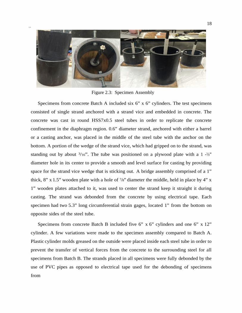
Figure 2.3: Specimen Assembly
Specimens from concrete Batch A included six 6” x 6” cylinders. The test specimens
consisted of single strand anchored with a strand vice and embedded in concrete. The
concrete was cast in round HSS7x0.5 steel tubes in order to replicate the concrete
confinement in the diaphragm region. 0.6” diameter strand, anchored with either a barrel
or a casting anchor, was placed in the middle of the steel tube with the anchor on the
bottom. A portion of the wedge of the strand vice, which had gripped on to the strand, was
standing out by about 3/16”. The tube was positioned on a plywood plate with a 1 -3⁄8”
diameter hole in its center to provide a smooth and level surface for casting by providing
space for the strand vice wedge that is sticking out. A bridge assembly comprised of a 1”
thick, 8” x 1.5” wooden plate with a hole of 7/8” diameter the middle, held in place by 4” x
1” wooden plates attached to it, was used to center the strand keep it straight it during
casting. The strand was debonded from the concrete by using electrical tape. Each
specimen had two 5.3” long circumferential strain gages, located 1” from the bottom on
opposite sides of the steel tube.
Specimens from concrete Batch B included five 6” x 6” cylinders and one 6” x 12”
cylinder. A few variations were made to the specimen assembly compared to Batch A.
Plastic cylinder molds greased on the outside were placed inside each steel tube in order to
prevent the transfer of vertical forces from the concrete to the surrounding steel for all
specimens from Batch B. The strands placed in all specimens were fully debonded by the
use of PVC pipes as opposed to electrical tape used for the debonding of specimens
from

19
Batch A. Two 1/2” diameter holes were drilled 1” from the top of the steel tubes in order to
facilitate the moving of specimens, while ensuring a tight fit of the mold against the steel
tube. This is shown in Figure 2.3. Six strain gages were placed on each 6” x 6” specimen
− two 5.3” long circumferential gages, located 1” from the bottom of the steel cylinder on
opposite sides of the specimen, and two circumferential and two vertical 0.2” long strain
gages, located 2” from the bottom of the specimen above the 5.3” long circumferential
gages. Twenty-two 0.2” long strain gages were placed on the 6” x 12” specimen − 11
circumferential and 11 vertical. Since all of the vertical gages would not fit at once, the
gages were placed in two parallel lines of 6 and 5 gages, respectively. The strain gage
configurations are shown in Figure 2.2, where the circumferential gages are represented by
circles and the vertical gages are represented by vertical line segments.
After casting, the specimens were turned upside down, such that the strand vice was on
top; then, a hydrostone layer of approximately 0.7” thickness was cast under each
specimen, in order to create a level surface during testing. This is shown in Figure 2.4.
Figure 2.4: Hydrostone Pouring
2.3 Testing Procedures
The specimens were initially tested by loading a strand, which was engaged in a chuck, in
tension as discussed in Subsection 2.3.1. However, assuming the strand anchor is stronger
than the strand and the (desired) ductile failure mode would be achieved by the fracture of
the

20 ``
strand, performing only tension tests would stand in the way of obtaining knowledge
about the capacity of the strand vice. Also, since the location of interest is the area of
concrete bearing on the bottom face of the anchor inside the cylinder, the forces are
transferred such that the bottom anchor surface, and the strand vice wedge, located on the
opposite side of the anchor, would both be under compression regardless of whether a
tensile load is applied through pulling the anchored strand, or a compressive load is
applied directly on the chuck body. Thus, it was deemed appropriate to test the anchors in
compression in order to determine their capacity.
2.3.1 Tension Tests
The tension test setup is shown in Figure 2.5.
(a) (b)
Figure 2.5: Tension Test Setup
A 1/4” thick rectangular plate was placed on top of each 6” x 6” specimen, then a
hollow 6” long, 6” ID steel tube was placed above that. A 1-1⁄2” thick 7” x 7” steel plate
was placed

21
on top of the supporting hollow tube. The specimens were then placed on top of wooden
blocks, in order to be lifted high enough for the plate to fit underneath the bottom Baldwin
head. Then, a multiuse strand vice was attached to the free end of the strand and caught in
between the top Baldwin head clamps. The tensile load was applied by moving the top test
head and the lowest surface up simultaneously. Two potentiometers were glued on the
strand. Two specimens from concrete Batch B were tested in tension.
2.3.2 Compression Tests
The schematic compression test assembly for specimens from concrete batch A is shown
in Figure 2.6.
Figure 2.6: Schematic Compression Test Assembly Batch A
In all cases a gap was left below the steel cylinder, with the goal of ensuring that the
steel cylinder provided only radial stress to confine the concrete by preventing the transfer
of vertical stresses from the concrete along the walls of the steel cylinder. To achieve the
gap, the concrete was supported on a pad of hydrostone − a quick-setting high strength
paste. The hydrostone was also cast in order to provide a level bottom surface for the
specimens.
The load application assembly changed slightly between tests, until the best method
was decided on. The initial testing procedure was as follows. All specimens were placed
on the testing machine sitting on the hydrostone with the anchors (barrel or casting) on
top. While

22 ``
testing the first specimen, a 1-3⁄4” diameter Williams rod (fu = 150 ksi) with a nut was
used to apply the compression load directly on the wedge of the strand vice. The rod was
centered by a bridge assembly comprised of a 2” thick, 8” x 4.5” wooden plate with a hole
of 1-7⁄8” diameter the middle, held in place by 4” x 2” wooden plates attached to it. Two
potentiometers were attached to the rod in order to measure the anchor displacement
during the test.
The loading assembly was changed at the end of the first test, since part of the
deformation measured was due to the wedge (which was standing out by about 3/16”) being
pushed into the chuck. A 1-1⁄4” diameter ASTM A490 nut was placed over the chuck body,
covering the wedge and the 1-3⁄4” rod was placed on top of the nut, in which manner the
load would be applied onto the chuck body alone. The nut served as a high-strength tube
through which the load was delivered to the barrel (and not the wedge) of the strand
vice.
At the end of the second test, the 1-3⁄4” Williams rod, as well as the 1-1⁄4” ASTM A490
diameter nut beneath it used to apply the load had both yielded and deformed. Hence, the
final version of the loading assembly was to place a 3/4” thick plate between the loading
rod and the 1-1⁄4” diameter A490 nut. The damage (by local yielding) was then limited to
the plate, and this resulted in maintaining the alignment of the load train components.
Push tests were carried out on all six 6” x 6” specimens from concrete Batch A. The variations in the test assemblies for Batch A specimens are shown in Table 2.4.

23
Table 2.4: Batch A Test Setup Variations
In the first series of tests, discussed above, the displacements measured were partly
due to the yielding of the loading rod, nut and plate, as well as the chuck top surface.
Thus, a new testing assembly was created for the specimens from batch B as shown in
Figure 2.7.

24 ``
Figure 2.7: Schematic Compression Test Assembly Batch B
The initial test setup was as follows. A hollow 6” long, 6” ID supporting steel tube
with a hole in the side was placed on the test machine surface. A 1-1⁄2” thick, 7” x 7” steel
plate with a 1-1⁄2” diameter hole in the middle was placed on top of the hollow steel tube.
The test specimen was placed on top of the 1-1⁄2” thick steel plate, with the strand
extending down the hole and into the supporting tube by approximately 6”. Two
potentiometers were glued to the strand in the hollow tube, their wires extending through
the holes in the supporting tube. The purpose was to measure the movement of the body of
the strand vice relative to the concrete, without including the deformation of the load
train. The strand acted as a push rod for the potentiometers. The potentiometers rested on
a plate with 1⁄2” thickness, placed in the middle of the supporting tube on the bottom of
the assembly.
In order to ensure that the load is being applied to the chuck body and wedge
simultaneously, replicating the actual loading scenario as closely as possible, a piece of
high strength rod with four 1 -1⁄4” diameter A490 nuts tightened onto it (nut-rod loading
assembly) was used to apply the load. The 3⁄4” thick plate, connected to the Baldwin was
placed on top. The nuts were kept in place by a bridge assembly comprised of a 2” thick,
8” x 4.5” wooden plate with a hole of 1 7⁄8” diameter the middle, held in place by 4” x 2”
wooden plates attached to it. Two potentiometers were attached to the nut-rod loading
assembly in order to measure

25
the chuck displacement during the test.
Since the potentiometers detached from the 4 A490 nut - high strength rod loading
assembly during the course of the test, it was decided to include 5 A490 nuts for the
second compression test. Furthermore, since the steel plate, used between the supporting
tube and the testing specimen had a hole larger than the 0.6” strand diameter, a sort of
concrete flow was observed during the test, as the concrete crushed through the hole in the
plate. This is discussed in detail in Section 2.4. Hence, a 1⁄4” thick rectangular plate with 13⁄16” diameter hole was used, to minimize the space around the strand. This revised test
setup was used for the 6” x 12” specimen.
Push tests were carried out on three 6” x 6” specimens, as well as on the 6” x 12”
specimen from concrete Batch B.
The variations in test setups for batch B are summarized in Table 2.5.
Table 2.5: Batch B Test Setup Variations

26 ``
2.4 Test Results The results from all compression and tension tests are summarized in Table 2.6.
Table 2.6: Confined Anchorage Test Results
It should be noted that even though the loads are referred to as ’ultimate load’,
that does not mean load at failure, just the maximum applied load for each test. The
anchor displacement values were measured after the tests were concluded by using a
caliper. It should be noted that these displacements roughly reflect the rigid body motion
of the strand vice, excluding the deformations due to yielding of the loading assembly
and are not the same as the displacements of the testing assembly, which were recorded
by potentiometers.
The specimens for which no plastic mold was used to debond the concrete from the
steel tube (Specimens CBA and CCA 1,2 and 3), a barrel anchor displacement of about
0.25” corresponding to a load of about 200 kips was recorded. Specimens, for which
greased plastic molds were used to debond the concrete from the surrounding steel tube
(specimens CBA 5-6), a barrel anchor displacement of about 0.66” for a load of about 200
kips was measured. The reason behind the high barrel anchor displacement of 1.5” for
specimen CBA 4, which also included a greased plastic mold, is discussed later in detail.

27
The casting anchor displacements were much smaller compared to barrel anchors, which
is to be expected due to the much higher bearing area.
2.4.1 Tension Test Results
The barrel anchor specimens post-tension tests are shown in Figure 2.8.
(a) TBA 1 (b) TBA 2
Figure 2.8: Barrel Anchor Tension Test Specimens
Both specimens failed due to strand fracture prior to the occurrence of any damage
to the strand anchor or the surrounding concrete.
2.4.2 Compression Test Results
The barrel anchor compression test specimens post testing are shown in Figures 2.9a to 2.9f.
28 ``
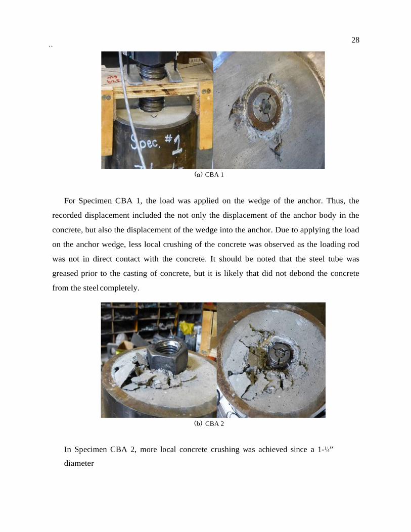
(a) CBA 1
For Specimen CBA 1, the load was applied on the wedge of the anchor. Thus, the
recorded displacement included the not only the displacement of the anchor body in the
concrete, but also the displacement of the wedge into the anchor. Due to applying the load
on the anchor wedge, less local crushing of the concrete was observed as the loading rod
was not in direct contact with the concrete. It should be noted that the steel tube was
greased prior to the casting of concrete, but it is likely that did not debond the concrete
from the steel completely.
(b) CBA 2
In Specimen CBA 2, more local concrete crushing was achieved since a 1-1⁄4”
diameter

29
A490 nut was used to apply the load on the chuck body, as opposed to the anchor wedge.
The loading nut and rod yielded by the end of the test. The steel tube was greased prior to
concrete casting.
(c) CBA 3
In Specimen CBA 3, a 3/4” plate was added on top of the loading 11⁄4” diameter A490
nut in order to prevent it from yielding. The load was still applied to the anchor body and
approximately the same amount of local crushing as in 2.9b was observed. The steel tube
was greased prior to concrete casting.
(d) CBA 4
Beginning with Specimen CBA 4, and continuing through Specimen CBA 6, the
concrete was cast in plastic molds, placed in the greased steel tube in order to debond
the concrete

30 ``
from the tube and prevent the transfer of axial stresses from the concrete through the steel
tube. The goal was that the tube would only act as a confining presence and all the vertical
stress would all pass down through the concrete, without axially engaging the tube. Two 1⁄2” diameter holes were drilled 1” from the top of each specimen, in order to ensure a tight
fit between the plastic mold and the surrounding steel tube. Similarly, for Specimens CBA
4, 5 and 6, the load was applied y using a high strength threaded rod with A490 nuts as
shown in Figure 2.7. A supporting steel tube was used as shown in Figure 2.7. An
assembly comprised of a high-strength rod with (4) 1-1⁄4” diameter A490 nuts was used to
apply the load. Two of them locally crushed the concrete, embedding themselves in it
completely, while displacing the anchor significantly. This happened due to the fact that a
1-1⁄2” thick plate with a 1-1⁄2” diameter hole in the middle was used between the specimen
and the supporting tube, which lead to a concrete flow through the 1-1⁄2” plate hole as
illustrated in Figure 2.9.
Figure 2.9: Specimen CBA 4 Concrete Flow

31
It should be noted that the concrete around the barrel anchor was removed in order
to examine what had occurred beneath the anchor. A region of concrete shaped like a
washer with an approximate thickness of 2 mm was discovered directly underneath the
anchor. Other than that, the concrete around and under the anchor appeared to be
undamaged.
(e) CBA 5
(f) CBA 6
Figure 2.9: Barrel Anchor Compression Test Specimens
In order to prevent the concrete flow observed in Figure 2.9d, a 3/4” thick plate was added

32 ``
on top of the 1-1⁄2” thick plate in the loading assemblies of Specimens CBA 5 and CBA 6.
Thus, the local crushing of the concrete was less severe, as its vertical displacement
capacity was inhibited. The local crushing is still more severe when compared to Figures
2.9b and 2.9c, due to the presence of the supporting tube, as well as the debonding of
concrete.
The casting anchor specimens after compression tests are shown in Figure 2.10.
(a) CCA 1 (b) CCA 2 (c) CCA 3
Figure 2.10: Casting Anchor Compression Test Specimens
The steel tube was greased prior to concrete casting but no plastic mold was used. The
load was applied to the anchor body via A490 nuts and no local crushing was observed at
the end of any of the casting anchor tests.
2.5 Analysis of Results
2.5.1 Summary of Results The loads obtained from all barrel anchor tests are shown in Figure 2.11. Since the
maximum loads obtained from the casting anchor tests were very close to the barrel
anchor maximum loads, they don’t provide any additional contribution. Furthermore, the
casting anchors have large dimensions and are much heavier, thus the use of barrel
anchors would be preferred for facilitation of constructability.

33
Figure 2.11: Barrel Anchor Tests Summary
The maximum loads, obtained from the barrel anchor compression tests were
around 4-4.5 times the fracture load of the strands. Even under these high loads
very little local crushing was observed and he tests were stopped because of
yielding in the steel load train. Thus, it was deemed appropriate to further
investigate this phenomenon.
The main quantities of interest obtained from the barrel anchor and casting
anchor tension and compression tests, respectively, are summarized in Tables 2.7
and 2.8.

34 ``
Table 2.7: Analysis of Barrel and Casting Anchor Tension Test Results
Table 2.8: Analysis of Barrel and Casting Anchor Compression Test Results
The ratio between the bearing stress and lateral confining stress for each test, as shown
in Tables 2.7 and 2.8, is important in evaluating the effectiveness of the confinement. The
bearing stress was obtained from the peak load and the contact area between the anchor
and the concrete, which was 1.94 in2 for the barrel anchors and 17.18 in2 for the casting
anchors. The lateral confinement stress was obtained from the stress in the steel tube,
which was, in turn, obtained from the strain gage readings, using 3-D Hookes law as
shown in Equation 2.5.
𝜎𝜎𝜃𝜃 = 𝐸𝐸𝑠𝑠
(1 + 𝜈𝜈)(1− 2𝜈𝜈) [(1− 𝜈𝜈)𝜖𝜖𝜃𝜃 + 𝜈𝜈(𝜖𝜖𝑏𝑏 + 𝜖𝜖𝑧𝑧)] 2.5
where subscripts r, θ and z refer to the radial, circumferential and axial directions,

35
respectively. Specimens CBA 1,2 and 3 had a pair of circumferential gages on opposite
sides, located at 5” from the top of the specimen on the outside of the steel surface. The
vertical strains for those specimens were determined by using 3-D Hooke’s Law,
assuming σθ = 0 as shown in Equation 2.6.
0 = (1 − 𝜈𝜈)𝜖𝜖𝑏𝑏 + 𝜈𝜈(𝜖𝜖𝜃𝜃 + 𝜖𝜖𝑧𝑧) 2.6
𝜖𝜖𝑏𝑏 = −𝜈𝜈
1 − 𝜈𝜈[𝜖𝜖𝜃𝜃 + 𝜖𝜖𝑧𝑧 ]
Specimens CBA 4 and 5 had a pair of circumferential gages, located 5” from the top of
the specimen, and a pair of circumferential strain gages, as well as a pair of vertical strain
gages, located at 4” from the top of the specimen.
Assuming a thin walled cylindrical pressure vessel,
𝜎𝜎𝜃𝜃 =𝑝𝑝𝑝𝑝𝑡𝑡
2.7
where p is the internal pressure, which is in this case the lateral confining stress, f’ L ,
R = 3 in is the internal radius of the steel tube,
t = 1/2 in is the thickness of the steel tube.
The lateral confining stress on the concrete is equal to the radial stress at the inner
surface of the steel cylinder and is given by Equation 2.8.
𝑓𝑓 𝐿𝐿′ = 𝜎𝜎𝑏𝑏 =
𝑡𝑡𝜎𝜎𝜃𝜃𝑝𝑝
2.8
Concrete is commonly treated as satisfying a Mohr-Coulomb failure criterion, in
which case
𝑓𝑓𝑐𝑐𝑐𝑐 = 𝑓𝑓 𝑐𝑐′ + 𝑐𝑐𝐿𝐿𝑓𝑓 𝐿𝐿′ = 𝑓𝑓 𝑐𝑐′ + �
1 + 𝑠𝑠𝑠𝑠𝑠𝑠𝑠𝑠1 − 𝑠𝑠𝑠𝑠𝑠𝑠𝑠𝑠
� 𝑓𝑓 𝐿𝐿′ 2.9
where φ is the internal angle of friction.
Selecting φ = 37° returns the result found experimentally by Richart, Brandtzaeg and
Brown shown in Equation 2.11 (Richart et al., 1929).
𝑓𝑓 𝑏𝑏𝑏𝑏𝑏𝑏𝑏𝑏𝑏𝑏𝑏𝑏𝑏𝑏′ = 𝑓𝑓 𝑐𝑐′ + 4.1𝑓𝑓 𝐿𝐿
′ 2.10

36 ``
The coefficient cL indicates the effectiveness of the confinement which, according to
the Mohr-Coulomb theory, depends on the internal friction angle. For each test result, a
value of cL can be calculated by treating the bearing stress as the confined concrete
strength, to give
𝑐𝑐𝐿𝐿 =𝑓𝑓𝑏𝑏𝑏𝑏𝑏𝑏𝑏𝑏𝑏𝑏𝑏𝑏𝑏𝑏′ − 𝑓𝑓 𝑐𝑐′
𝑓𝑓 𝐿𝐿′ 2.11
Values of cL are given in Tables 2.7 and 2.8 and may be compared with the 4.1 found
by Richart et al. (1929). For the barrel anchors tested in tension, the comparison is not
really valid, because the concrete had not started to crush significantly by the time the
strand failed and the test was stopped. Thus, the resisting mechanism was still partially
elastic, and was not the sliding shear one that underlies the Mohr-Coulomb theory. The cL
values for the casting anchors are comparable to those found by Richart et al. (Richart et
al., 1929). The cL values for the barrel anchors tested in compression are about an order
of magnitude higher than Richart’s, which suggests that other beneficial mechanism, in
addition to than conventional confinement, was active. It is believed that the bearing stress
was high because the bearing load was applied over only a small proportion of the total
available area. Even though this behavior has been seen before (Hawkins, 1968) and is
incorporated in codes (ACI318 (2011) Chapter 10 and Appendix D), good mechanical
models for it are not yet available.
Even though these cL values from the bearing anchor compression tests are high, they
are still lower bounds, because the bearing stress measured in the test was a lower bound
to the true failure stress. The tests had to be stopped because the ASTM A490 nut and the
Williams bar used in the load train were deforming plastically, and not because the
concrete was failing.
The strains in the steel tube varied over the height of the tube. This was seen in
Specimen CBA 6, which was 12” high, and was equipped with 11 circumferential and 11
vertical strain gages, measuring the strains at every inch along the height of the steel tube.
However, for different specimens, the strains had to be read where gages were available.
In specimens

37
CBA 4 and CBA 5 (6” high), the hoop strains were taken as the average of gage readings
5” and 4” from the top of the specimen, respectively; and the vertical strains were taken as
the average of the gage readings 4” from the top of the specimen. Those heights were
approximately where the maximum strains were observed.
Specimens CBA 1, 2 and 3 were also constructed with 6” high tubes, with only
circumferential gages 5” from the top of the specimen and were placed there because that
location was expected to experience approximately the maximum strain. The lateral
confining stress is thus a local value at the inside of the steel tube, at approximately the
location of the maximum value, and so some variation in results should be expected.
However, the average value was 33, with a Coefficient of Variation of 17%.
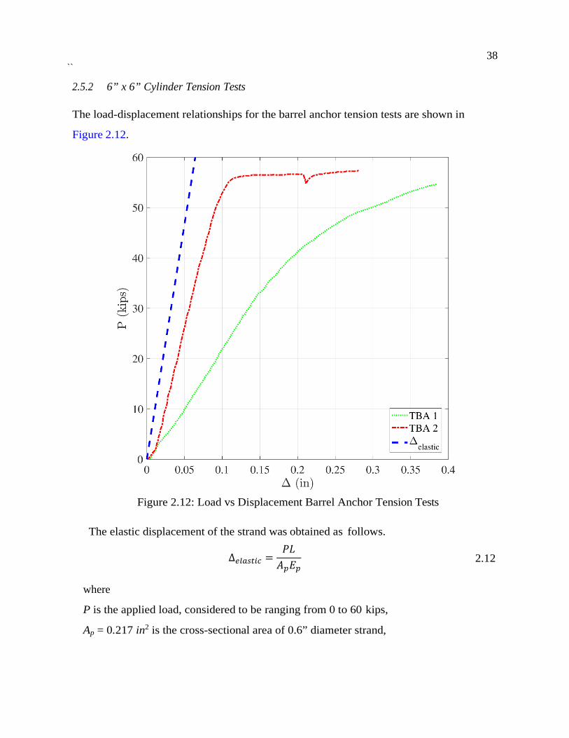
38 ``
2.5.2 6” x 6” Cylinder Tension Tests The load-displacement relationships for the barrel anchor tension tests are shown in
Figure 2.12.
Figure 2.12: Load vs Displacement Barrel Anchor Tension Tests
The elastic displacement of the strand was obtained as follows.
Δ𝑏𝑏𝑒𝑒𝑏𝑏𝑠𝑠𝑒𝑒𝑏𝑏𝑐𝑐 =𝑃𝑃𝑃𝑃𝐴𝐴𝑝𝑝𝐸𝐸𝑝𝑝
2.12
where
P is the applied load, considered to be ranging from 0 to 60 kips,
Ap = 0.217 in2 is the cross-sectional area of 0.6” diameter strand,

39
Ep = 28000 ksi is the modulus of elasticity of the strand,
L = 6.5 in. is the length of the strand
Thus, the elastic displacement of 0.6” diameter strand would be 0.06” at about 55 kips,
resulting in a plastic deformation of about 0.05” for TBA 2 and 0.29” for TBA 1. Specimen
TBA 1 was subjected to two loading cycles. During the first loading cycle, a test setup
malfunction took place preventing strand fracture from occurring. Consequently, a second
loading cycle was conducted, during which strand fracture was achieved. However, while
the stiffness of Specimen TBA 1 was drastically reduced, the ultimate strand capacity was
similar to that of Specimen TBA 2.
2.5.3 Compression Tests The displacement values obtained from the potentiometers during the tests are shown by
illustrating the load-displacement relationship for all compression tests in Figure 2.13.

40 ``
Figure 2.13: Load vs Average Displacement Compression Tests
The displacements for the bonded barrel anchor specimens CBA 1, CBA 2 and CBA
3 are around 0.4” for the maximum load; however it should be kept in mind that part of
the displacement detected by the potentiometers was due to the yielding of the nut and
rod loading assembly, as well as due to the yielding of the chuck top surface. Thus, the
displacements of the chuck body relative to the concrete would be smaller. If one is to
consider a load of about 60 kips (which would be the failure load in practice), the largest
displacement, which occurred for specimen CBA 1 is about 0.07”.
The debonded barrel anchor specimens, namely, CBA 4, CBA 5 and CBA 6, experience

41
much larger displacements at the maximum load level. The reason why the maximum ob-
served displacement for specimen CBA 4 is about 0.5” is because when the concrete flow
occurred, the instruments recording the displacement were damaged.
Overall, the maximum displacements were larger due to the debonding of the concrete
from the steel tube, by the use of plastic molds. This allowed radial displacement of the
concrete to occur where any gaps between the plastic mold and the steel tube may have
existed. This behaviour was confirmed by the fact that oil squeezed through the gap
between the plastic mold and the steel tube during the tests. Furthermore, the debonding
also allowed the free top concrete surface around the anchor to heave more easily when
compared to bonded specimens.
The displacement at a load of about 60 kips (which would be the failure load in
practice) are about 0.15” - 0.2”, proving the barrel anchor performance is satisfactory and
indicating that this detail does not only have sufficient capacity in terms of strength, but
will also not experience significant slipping.
It should be noted that for the bonded barrel anchor specimens CBA 4, CBA 5 and
CBA 6, a pair of potentiometers were attached to each A490 nut in the load train, and to
each strand as shown in Figure 2.7. The displacement values recorded for the nuts and
the strands were very close as shown in Figure 2.14.

42 ``
Figure 2.14: Load vs Average Displacement Debonded Barrel Anchor Specimens
The potentiometers glued to the A490 nuts used for loading and the ones glued to the
strands gave similar results, leading to the conclusion that the obtained displacements
were reasonably well captured.
It should be noted that Specimens CBA 1, CBA 2, CBA 3, CCA 1, CCA 2 and CCA 3
had only two potentiometers, attached on the 1-1⁄4” diameter Williams nut, used to apply
the load as shown in Figure 2.6.
Ultimately, the use of the nut displacement values was deemed appropriate for all

43
compression specimens.
The load-strain relationships for all compression tests are shown in Figure 2.15.
Figure 2.15: Load vs Average Hoop Strain Compression Tests
As previously mentioned, the casting anchor hoop strains are approximately half of the
barrel anchor specimens’ strains. They are certainly expected to be smaller, because the
distribution of load at the point of application is more uniform, however, computing the
expected ratio would be complicated.
The average strain values for the bonded specimens CBA 4, CBA 5 and CBA 6 were
similar to those obtained from the other barrel anchor tests. The jump that occurs at about 108
kips for specimen CBA 4 could have been caused by the concrete flow; a sudden drop in

44 ``
the load took place possibly as the concrete started squeezing out and after several seconds,
the specimen started picking load again.
It should be noted that for Specimens CBA 4 and CBA 5 (6” x 6”), unbonded with the
use of plastic cylinder molds, only the long circumferential strain gage readings were used,
when comparing their behaviour to the bonded Specimens CBA 1, CBA 2, CBA 3, CCA
1, CCA 2, and CCA 3 (6” x 6”). This was done for the sake of consistency between results.
The long and short hoop strain values were fairly close for Specimens CBA 4 and CBA 5 as
shown in Figure 2.16.
Figure 2.16: Load vs Average Hoop Strain CBA 4 and CBA 5

45
Specimen CBA 6 (6” x 12”) had 11 small circumferential and 11 small vertical strain
gages, placed along every inch of the steel tube. Thus, the circumferential and vertical
gage readings at 5” from the top surface of the specimen were used in order to compare
the results with the rest of the compression tests, since all of the strain gages in all of the
other (6” x 6”) specimens were located 4” and 5” from the top of the specimens.
The load vs. lateral confining stress curves for all specimens are shown in Figure 2.17.
This behaviour is consistent with the load vs strain curves, since the lateral confining
pressure was derived from the recorded circumferential strain.
Figure 2.17: Lateral Confining Stress vs Load Compression Tests
The confinement coefficient-load relationships for all compression tests are shown in Figure 2.18.

46 ``
Figure 2.18: Confinement Coefficient vs Load Compression Tests
The steel tube provides very small resistance at low loads, the higher the load applied,
the more confining stress can be obtained. When the confinement ratio is plotted versus
the load, it can be seen that for casting anchors, the ratio is converging to 4, while for
barrel anchors, it is approaching a maximum of 40 at high loads for Specimens CBA 1, 2
and 3 without plastic molds and a maximum of 33 for Specimens CBA 4,5 which
included plastic cylinder molds. Because two features (cylinder height and steel-concrete
bond) were different in the two cases, it is not possible to tell which feature affected the
results the most.
Specimen CBA 6 was constructed with a 6” x 12” cylinder and had 11 circumferential and

47
11 vertical strain gages, in order to determine the distribution of stresses in the concrete
more accurately. The axial and circumferential stress values were determined from the
measured vertical and circumferential strains at every inch along the height of the
specimen, and the stress profiles along the cylinder height at three different load levels
(150, 175 and 200 kips) are shown in Figure 2.19.
(a) (b)
Figure 2.19: Axial and Hoop Stress Profiles Along Height for Specimen CBA 6
Several features are apparent in all three plots.
• Peak Hoop Stress. The peak hoop stress occurs at about 8” up from the bottom,
or 2” below the loading interface at the bottom of the chuck. This suggests that
the load is transferred outwards from its point of application in a conical strut
structure with an outer surface that is at 45°to the vertical. That implied load
transfer mechanism is in agreement with the expected strut-and-tie model. The
hoop stress remains above

48 ``
50% of that maximum value over a 4” wide band, centered on the location of the
peak stress. This suggests a fan mechanism, rather than a pure cone.
• Non-zero Vertical Stress. The vertical stress is non-zero over essentially the whole
height. This suggests that either the tube wall was bending or that some axial stress
was being transferred to the tube wall by friction, despite the greased plastic liner.
If the radial pressure from the concrete on the tube was non-uniform with height,
which was almost certainly the case, then some wall bending was inevitable. The
fact that the peak vertical stress occurred close to the location of peak hoop stress
supports this view.
• Negative Vertical Stress. The vertical stress is negative near the base. This radial
stress there was expected to be nearly uniform with height, and that is confirmed by
the nearly-constant hoop stresses, in which there should be little bending. The
vertical stress is therefore attributed to axial stress in the tube wall. That vertical
stress is in the range of 2-5 ksi from 2”-6” above the base, decreasing gradually
towards the bottom, and it drops sharply to a value close to zero right at the bottom.
This suggests that some friction existed between the tube wall and the concrete,
despite the efforts to eliminate it with the greased plastic sleeve.
In order to investigate further the internal stresses, and particularly the bending, a
finite element numerical model of the system was created using ABAQUS software. The
following features were included in the model:
• The 1/2” thick, 6” ID steel cylinder was investigated in the model, concrete was not
included.
• Generalized Hooke’s Law was used to determine the radial strains along the height
of the specimen, using the axial and circumferential strain values along the
specimen height obtained during testing, as well as to determine axial and hoop
stresses.
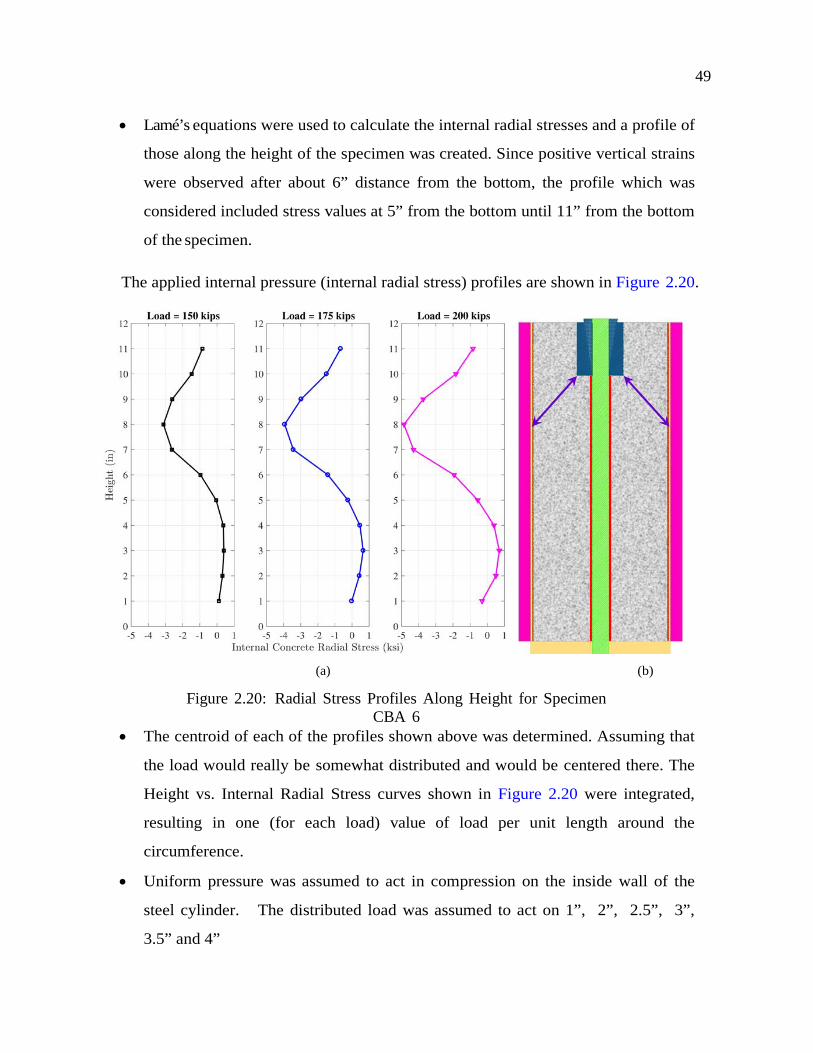
49
• Lamé’s equations were used to calculate the internal radial stresses and a profile of
those along the height of the specimen was created. Since positive vertical strains
were observed after about 6” distance from the bottom, the profile which was
considered included stress values at 5” from the bottom until 11” from the bottom
of the specimen.
The applied internal pressure (internal radial stress) profiles are shown in Figure 2.20.
(a) (b)
Figure 2.20: Radial Stress Profiles Along Height for Specimen CBA 6
• The centroid of each of the profiles shown above was determined. Assuming that
the load would really be somewhat distributed and would be centered there. The
Height vs. Internal Radial Stress curves shown in Figure 2.20 were integrated,
resulting in one (for each load) value of load per unit length around the
circumference.
• Uniform pressure was assumed to act in compression on the inside wall of the
steel cylinder. The distributed load was assumed to act on 1”, 2”, 2.5”, 3”,
3.5” and 4”

50 ``
wide strips and the value of the uniform pressure would be obtained by dividing the
load per unit length by the strip width being analyzed.
• To check the compatibility of the model with the experimental data, the measured
strain profiles along the height of the specimen for 125 kips, 150 kips, 175 kips and
200 kips were compared with the profiles obtained from the ABAQUS model. The
true width of the applied load band could be obtained by finding the curve in the
numerical simulation that the best-fitted the measured strains, and by inspecting the
measured and computed ratios of vertical to horizontal stress.
A comparison between the measured and computed strains on the outside of the steel
cylinder wall, at different load levels is shown in Figure 2.21. Analyses were conducted
for many different widths of the loading band, but only 2”, 3” and 4” are shown in the
interests of clarity. Both vertical and hoop strains are shown.

51
(a) External Steel Tube Circumferential Strain Profile
(b) External Steel Tube Vertical Strain Profile
Figure 2.21: Experimental Strain Profiles vs ABAQUS Strain Profiles

52 ``
The overall shapes of the computed profiles match those of the measured profiles, but
the hoop strains appear to fit better than the vertical strains. Note that no vertical load
on the steel was included in the numerical model, but friction might have introduced
some in the test, which may explain why the computed vertical strains are more
positive (tensile) than their measured counterparts, especially in the peak stress region.
The strain errors were squared, added and normalized with respect to load, for each
load width. The results are plotted against load width in 2.22b, which shows vertical (”V”)
and circumferential (”C”), or hoop, values separately. Results for the vertical and hoop
errors combined are shown in 2.22a.

53
(a) Individual Strain Difference Error
(b) Cumulative Strain Difference Error
Figure 2.22: Strain Difference Error vs Strip Width

54 ``
It can be deduced that the best fit is obtained with a load width between 3” and 4”.
The hoop strains showed smaller errors than the vertical ones, as might be expected from
the profiles in Figure 2.21, and the fits were generally better at lower loads (i.e. 150 rather
than 200 kips).
Other loading patterns, such as a triangular, a parabolic and a sinusoidal distribution
were considered; however, since the strain profile along the height of the specimen for the
uniformly distributed load pattern was always closest to the experimental profile, it was
concluded that investigating the uniform load distribution in more depth would be a
sufficient.
Figure 2.23 shows the best fit model based on the numerical analysis results.
Figure 2.23: Internal Pressure Distribution Based on Analysis Results
2.6 Conclusions
The use of an anchor with a small bearing area, namely a barrel anchor without a bearing
plate was deemed sufficient for the development of the girder- diaphragm connection
as a

55
result of the tests described in this chapter. It was shown that the barrel anchor detail
would have satisfactory capacity in terms of strength, while experiencing little slippage and
local crushing. When tested in tension, the barrel anchors had not sustained any damage
by the time the strand had reached its fracture load. Upon testing the barrel anchors in
compression, it was discovered the concrete directly behind the bearing anchor could resist
bearing stresses as high as 100 ksi with very little local crushing and little slip of the anchor.
Casting anchors’ behaviour under compression was satisfactory, however their use would be
practically challenging due to constructability issues and extra weight, which can be a
problem during girder transportation. They are also larger compared to the current detail,
which includes a 4” x 4” rectangular backing plate welded to a barrel anchor. They were
investigated as they are more convenient, since no extra welding is required. Thus, barrel
anchors would be used in the next stages of the project, when the behaviour of anchored
strands, extended from the girder into the diaphragm.

56 ``
Chapter 3
BREAKOUT TESTS
3.1 Introduction This chapter discusses the tension tests carried out on strands, anchored with post-
tensioning chucks and embedded in concrete blocks, in order to observe the impact of the
possible failure mechanisms of the aforementioned on the development of the girder-cap
beam positive moment connection.
There are four main failure modes for headed studs, subjected to tensile load. One
possibility of failure is due to the yielding and possibly fracture of the anchoring system
before the breakout of concrete takes place, which is a ductile mode of failure and is
desirable. Failure can occur due to pullout - which is the sliding of the anchor (either
partially or completely) from the concrete, and should be prevented at all cost. Another
alternative is a pullthrough failure, which involves the pullout of the anchor (or a part of
it), with the generation of a localized and relatively small breakout cone in close
proximity to the anchor. This failure mode is likely to take place for anchors that have
undergone excessive deformations and is mainly dependent on the quality of the
anchoring device, thus it is viewed as acceptable. Lastly, highly undesirable brittle modes
of failure could occur due to either substantial breakout or splitting of the concrete
member before the yielding of the anchoring device. Splitting failure would be highly
dependent on the spacing between anchors, as well as the edge distance of the anchors and
the member thickness (Fuchs et al., 1995). These possible failure modes are depicted in
Figure 3.1.

57
(a) Steel Failure
(b) Breakout Failure
(c) Pullout Failure (d) Splitting Failure
Figure 3.1: Failure Types of Anchors Under Tensile Load (Fuchs et al., 1995)
For the tests described here, the concrete breakout failure mode was assumed as
58 ``
the governing mechanism. Different block depths and strand patterns were considered, by
taking into account the strands extended from the girders into the cap beam and the
possible breakout cones that could occur.
The goal of these tests is to determine the embedment depth of the anchored strands
at which the failure mode shifts from brittle to ductile, and thus prevents the breakout of
concrete from being the controlling mechanism. To that end, an expression, providing the
strength of the system as a function of depth, was sought.
3.2 Mechanics of Breakout and Methods of Prediction
As previously mentioned, the specimens were designed in accordance with the procedures,
specified in ACI and PCI. Both design methodologies are based on the Concrete Capacity
Design (CCD) Method, developed by Eligehausen (Fuchs et al., 1995).
3.2.1 Concrete Capacity Design Approach The Concrete Capacity Design (CCD) method proposes the following methodology for de-
termining the concrete capacity of steel fastenings under tension load (Fuchs et al., 1995).
For fastenings subjected to tensile load, a conical failure surface inclined at about
35° with respect to the concrete member is assumed. This implies that the failure surface
would spread horizontally roughly three times the effective embedment depth (Fuchs et al.,
1995).
The following equation is proposed by the CCD Method for the cone failure load of
a single anchor, embedded in uncracked concrete and unaffected by edge effects or
overlapping cones.
𝑁𝑁𝑏𝑏𝑛𝑛 = 𝑘𝑘𝑏𝑏𝑐𝑐 �𝑓𝑓 𝑐𝑐′ ℎ𝑏𝑏𝑒𝑒1.5 3.1
where knc = k1 k2 k3 and k1, k2 and k3 are calibration factors.
The Concrete Capacity Design method proposes knc = 40 for cast-in-place anchors. As the
tests described here involve cast-in-place anchors, this value was used when comparing
failure loads obtained from the experiments and predicted failure loads.

59
Since the CCD method is based on rectangular prisms, variations in edge distances,
spacing between anchors, as well as different configurations of anchors (group effect) can be
easily incorporated.
For multiple anchors, the capacity of concrete can be determined by using the following
equation.
𝑁𝑁𝑏𝑏 =𝐴𝐴𝑁𝑁𝐴𝐴𝑁𝑁𝑛𝑛
𝑘𝑘𝑏𝑏𝑐𝑐 �𝑓𝑓 𝑐𝑐′ ℎ𝑏𝑏𝑒𝑒1.5 3.2
where ANo = 9 hef2and is defined as the projected area of one anchor at the concrete surface
unlimited by edge influences or neighboring anchors, idealizing the failure cone as a pyramid
with a base length of 3hef ,
AN is defined as the actual projected area at the concrete surface, assuming the failure
surface of the individual anchors as a pyramid with a base length = 3hef ,
Ψ2 = 1 for edge distance ≥ 1.5hef ,
Ψ2 = 0.7 + 0.3𝑏𝑏𝑒𝑒𝑏𝑏𝑏𝑏 𝑒𝑒𝑏𝑏𝑠𝑠𝑒𝑒𝑏𝑏𝑏𝑏𝑐𝑐𝑏𝑏
1.5ℎ𝑒𝑒𝑒𝑒 for edge distance ≤ 1.5hef ,
hef is the effective embedment depth, in this case measured from the top of the barrel
anchor.
The projected areas mentioned above are illustrated in Figure 3.2.

60 ``
Figure 3.2: Projected Areas for Different Anchors Subjected to Tensile Load (Fuchs et al.,
1995)
3.2.2 ACI Design Approach The test specimens were designed according to the procedure, described in Appendix D in
the ACI 318-11 Code.
As in the CCD model (Fuchs et al., 1995), the breakout strength of concrete is
determined by assuming a concrete failure prism with approximately 35° angle. Similarly,
the failure surface projects 1.5hef horizontally from the center of the anchors.
The breakout strength of a single anchor, as well as a group of anchors embedded in
concrete, assuming cracked conditions, are determined by the following equations,
respectively.
For a single anchor,

61
𝑁𝑁𝑐𝑐𝑏𝑏 =𝐴𝐴𝑁𝑁𝑐𝑐𝐴𝐴𝑁𝑁𝑐𝑐𝑐𝑐
Ψ𝑏𝑏𝑒𝑒,𝑁𝑁Ψ𝑐𝑐,𝑁𝑁Ψ𝑐𝑐𝑝𝑝,𝑁𝑁N𝑏𝑏 3.3
For a group of anchors,
𝑁𝑁𝑐𝑐𝑏𝑏𝑏𝑏 =𝐴𝐴𝑁𝑁𝑐𝑐𝐴𝐴𝑁𝑁𝑐𝑐𝑐𝑐
Ψ𝑏𝑏𝑐𝑐,𝑁𝑁Ψ𝑏𝑏𝑒𝑒,𝑁𝑁Ψ𝑐𝑐,𝑁𝑁Ψ𝑐𝑐𝑝𝑝,𝑁𝑁N𝑏𝑏 3.4
where
ANc is the projected concrete failure area of a single anchor or group of anchors that
shall be approximated as the base of the rectilinear geometrical figure that results from
projecting the failure surface outward 1.5hef from the center lines of the anchor, or in the
case of a group of anchors, from a line through a row of adjacent anchors;
ANc ≤ nANco, and n is the number of anchors in the group, resisting tension,
ANco = 9hef2 and is defined as the projected concrete failure area of a single anchor with
an edge distance ≥ 1.5hef ,
Ψec,N =1
1+2𝑒𝑒𝑁𝑁
′
3ℎ𝑒𝑒𝑒𝑒
is a modification factor for groups of anchors loaded eccentrically in
tension and
e’N is the eccentricity of the tensile force relative to the center of the anchor group.
In the tests described here, the load was applied concentrically, thus Ψec,N = 1.0,
Ψed,N = 1.0 for minimum edge distance ≥ 1.5hef and is defined as a modification factor
for edge effects for single anchors or anchor groups loaded in tension. In tests, described
here, every specimen had edge distance > 1.5hef
Ψc,N = 1.25 for cast-in-place anchors and is defined as the modification factor for
anchors located in a region of a concrete member where analysis indicates no cracking at
service load levels,
Ψcp,N = 1.0 for cast-in-place anchors and is defined as the modification factor for post-
installed anchors designed for uncracked concrete,

62 ``
𝑁𝑁𝑏𝑏 = 𝑘𝑘𝑐𝑐𝜆𝜆𝑏𝑏�𝑓𝑓 𝑐𝑐′
where
kc = 24 for cast- in anchors and its values were determined from a large database of
test results in uncracked concrete at the 5 percent fractile and were adjusted to cracked
concrete,
λa = 1.0 for normal weight concrete.
For embedment depths greather than 11 in, the expression for Nb including the hef1.5
term was determined to be too conservative and an alternative was proposed as shown
below.
For 11 in. ≤ hef ≤ 25 in.
𝑁𝑁𝑏𝑏 = 16𝜆𝜆𝑏𝑏�𝑓𝑓 𝑐𝑐′ ℎ𝑏𝑏𝑒𝑒5 3⁄ ,
and
hef is the effective embedment depth, in this case measured from the top of the barrel
anchor.

63
The projected areas mentioned above are shown in Figure 3.3.
Figure 3.3: Projected Areas for Different Anchors Subjected to Tensile Load (ACI318, 2011)
The test specimens were designed based on designating a target capacity and
determining the required embedment depth to achieve failure at the target load,
according to the ACI procedure, described above.
3.2.3 PCI Design Approach
The design method, described in PCI Design Handbook Chapter 6 was used as an
alternative while designing the test specimens, in order to make a comparison with the
failure loads predicted by ACI.
64 ``
The breakout concrete strength for studs loaded in tension can be determined as
shown in Equation 3.5.
𝑁𝑁𝑐𝑐𝑏𝑏 = 𝑁𝑁𝑐𝑐𝑏𝑏𝑏𝑏 = 𝐶𝐶𝑏𝑏𝑠𝑠𝐴𝐴𝑁𝑁𝐶𝐶𝑐𝑐𝑏𝑏𝑏𝑏Ψ𝑏𝑏𝑒𝑒,𝑁𝑁Ψ𝑏𝑏𝑐𝑐,𝑁𝑁 3.5
where
𝐶𝐶𝑏𝑏𝑠𝑠 = 3.33𝜆𝜆�𝑒𝑒 𝑐𝑐′
ℎ𝑒𝑒𝑒𝑒
AN is the projected surface area for a stud or group of studs,
hef is the effective embedment depth, in this case measured from the top of the barrel
anchor to the surface of the concrete block.
Ccrb = 1.0 assuming uncracked concrete, which was the case here.
λ is a modification factor reflecting the reduced mechanical properties of lightweight
concrete, and λ = 1.0 for the tests described.
The projected areas considered by PCI are shown in Figure 3.4.

65
Figure 3.4: Projected Areas for Different Anchors Subjected to Tensile Load (PCI,
2004)
This method is more conservative than the ACI method, as for anchors, embedded
deeper than 11 in, ACI proposes an adjusted equation, suggesting that the hef1.5 used to
determine the breakout capacity is too conservative, including the use of hef5/3, as
described in Subsection 3.2.2.
3.3 Test Specimens
3.3.1 Specimen Configuration Fourteen specimens with varying depths and strand configurations were designed in order
to observe the effect of embedment depth and collective impact of different groups of
strands on the breakout failure mechanism. Considering the girder strands extended into
the diaphragm, the failure mechanisms for four different strand patterns were investigated-
single strand, two

66 ``
strands, four strands in a line and four strands in a square.
The designed specimens, as well as the details of the considered strand patterns
considered are shown in Figure 3.5.
(a) (b)
Figure 3.5: Breakout Specimen Configuration
The naming system for the specimens should is explained below.
The first letter of the specimen name - either B or U - stands for the bond conditions of

67
the strands in the specimen, indicating whether the specimen is bonded or unbonded.
The subsequent number – 1, 2 or 4 - stands for the number of strands present in the
specimen.
The following letter - O, L or S - represents the pattern of the strands in the specimen,
and corresponds to one, line and square strand patterns respectively.
The final number represents the effective embedment depth of the strand anchors, in
inches. It should be noted that the effective embedment depth was considered as the
distance from the top of the barrel anchor to the concrete surface.
Thus, for instance, U 4 L 9.25 would describe an unbonded specimen with 4 strands in
a line, with 9.25 in. effective embedment depth.
It should be noted that the effect of bonded strands was investigated only for specimens
with a single strand. It was theorized that the bonded specimens would fail at lower loads,
presuming the failure would occur in stages, generating from top of the specimen, creating
cone- like breakout surfaces developing in stages, depending primarily on the bond
between the strand and the concrete. However, all strands were covered with electrical tape
for approximately 1 in - 1.5 in from the top of the strand chuck and the single strand
specimens were quite shallow overall- varying between 1.75 in and 6.5 in. The duct tape
was used in order to prevent concrete from getting between the strand and the barrel
anchor. Thus, it is likely that the smallest bonded specimens weren’t fully bonded and it is
uncertain whether the “true” bonded behaviour can be captured by investigating such small
depths. Test results show that the maximum loads for bonded and unbonded specimens are
quite close, and further investigation of the bond conditions on the failure load was not
carried out.
3.3.2 Specimen Design The strand orientations, investigated in the tests, were selected considering that certain
groups among the extended strands were in danger of suffering a breakout failure, unless
they were embedded into the diaphragm for a sufficient length. To that end, the strands
were embedded in concrete blocks with varying depths, to determine how much

68 ``
embedment is needed to provide ductile failure mode, while investigating how closely the
CCD, ACI and PCI methods agree with the test breakout load values at failure. The
majority of the strands were debonded by using a plastic PVC pipe.
The loads induced in each specimen are shown in Figure 3.6.
Figure 3.6: Breakout Specimen Loads
Tensile load was applied to the strands, embedded in concrete, concentrically, while
the distributed load, acting in compression, represents the effect of the support posts, used
in the tests, pushing down on the ends of the concrete blocks. The support posts were
placed such that they would not interfere with the occurrence of the predicted 35°
breakout cone. As it can be seen in Figure 3.6, the testing system that was used here
generated bending moments on the concrete blocks; the specimens were not under the
effect of pure tension. Thus, flexural and shear effects would also be present in addition to
the failure mechanisms mentioned above. To that end, all of the specimens were
reinforced with flexural steel on top, considering that they would be tested along their
diagonals, such that they could resist the largest negative bending moments that would
arise during the tests. It was aimed to prevent excessive flexural cracking, thus avoiding
failure of the specimens in an undesired mode- flexure. Using flexural reinforcement
would also partially replicate the heavily reinforced diaphragm, and confine the concrete
to some extent, when compared to the concrete in the diaphragm, thus it was deemed to
provide more realistic conditions. Shear reinforcement was not placed in order to prevent
its prohibition of the expected breakout cones.

69
3.4 Test Setup The test setup is shown in Figure 3.7.
Figure 3.7: Breakout Test Setup
A testing assembly composed of a loading beam, namely, 2 MC channels with two
pieces of 3.5 in. wide flat bar between them welded back to back, sitting on two square
HSS 5x5x3/8 support posts was used.
The tension tests were conducted by using a hydraulic ram; the applied load was
recorded both by a pressure sensor connected to the ram, as well as by a load cell. Multi-
use strand chucks were used above the hydraulic ram to conduct the tension tests.

70 ``
Four potentiometers were used to determine the displacements of the concrete surface
and the strands in the duration of the tests.
For specimens with single strand, two potentiometers were placed on the strand, and
two were used to measure the heaving of the concrete surface relative to a timber bridge
attached to the outer edge of the block as shown in Figure 3.7.
For specimens with multiple strands, one potentiometer was used for each strand and
two were used to measure the concrete surface displacement.
Since the sizes of the blocks varied significantly, different setups were used for smaller
and larger specimens.
3.4.1 Small Specimens
The testing assembly for small specimens is shown in Figure 3.8.
Figure 3.8: Small Specimens Test Assembly
For smaller specimens, namely, ones with shallow depths and (mostly) a single strand,
the use of 2 MC6x15.1 channels was determined to be sufficient. The loading beam,
composed of the channels, resting on rectangular HSS posts was placed along the
diagonal of each

71
concrete block in order to maximize the post spacing and minimize the possibility of the
posts’ interfering with the breakout failure.
The channels were designed so that the spacing of the HSS posts could be adjusted to
any desired distance, and the pair of MC6x15.1 was chosen to satisfy bending and shear
requirements for a load of 60 kips at the widest spacing. A hydraulic ram with 60 kips
load capacity, as well as a load cell with 50 kips capacity were used in the tests.
As can be seen in Figure 3.8, plywood shims were placed under the HSS sections, in
order to prevent local crushing failure of a high spot of the concrete. It should also be
noted that the distance between the HSS sections was arranged such that the latter do not
restrict the predicted breakout cone, overlapping with its diameter. The procedures for
design of the breakout cone diameter are explained in detail in Section 3.2.
3.4.2 Large Specimens
The testing assembly for large specimens is shown in Figure 3.9.
Figure 3.9: Large Specimens Test Assembly
For the larger specimens, 2 MC 18x58 were used, because the larger spans and expected

72 ``
breakout forces of the four-strand specimens led to much larger moments.
A hydraulic ram and load cell with 300 kips capacity were used in the tests.
Plywood shims were placed under the HSS sections to prevent local crushing failure,
analogous to the small specimens’ assembly. Similarly, the distance between the HSS
sections was selected such that the predicted breakout cone would not be obstructed.
A piece of plywood was placed between the steel plates, located above the load cell
and below the multi-use strand chucks, in order to ensure that the wedges in the mutli-use
chucks were set the same amount, which would lead to all of the strands being stressed
simultaneously and the applied load being distributed identically among them.
3.5 Test Results
The loads at failure and the failure modes are shown in Table 3.1.
Table 3.1: Breakout Tests Results
For shallow specimens, namely, specimens with single strand and two strands, a
breakout failure mechanism similar to what was expected was achieved.
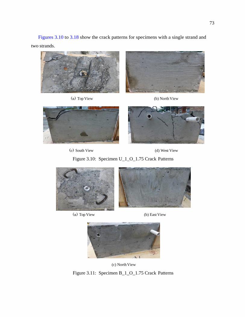
73
Figures 3.10 to 3.18 show the crack patterns for specimens with a single strand and
two strands.
(a) Top View (b) North View
(c) South View (d) West View
Figure 3.10: Specimen U_1_O_1.75 Crack Patterns
(a) Top View (b) East View
(c) North View
Figure 3.11: Specimen B_1_O_1.75 Crack Patterns

74 ``
(a) Top View (b) South View
(c) East View (d) North View
Figure 3.12: Specimen U_1_O_3.63 Crack Patterns
(a) Top View (b) East View
(c) South View
Figure 3.13: Specimen B_1_O_3.5 Crack Patterns
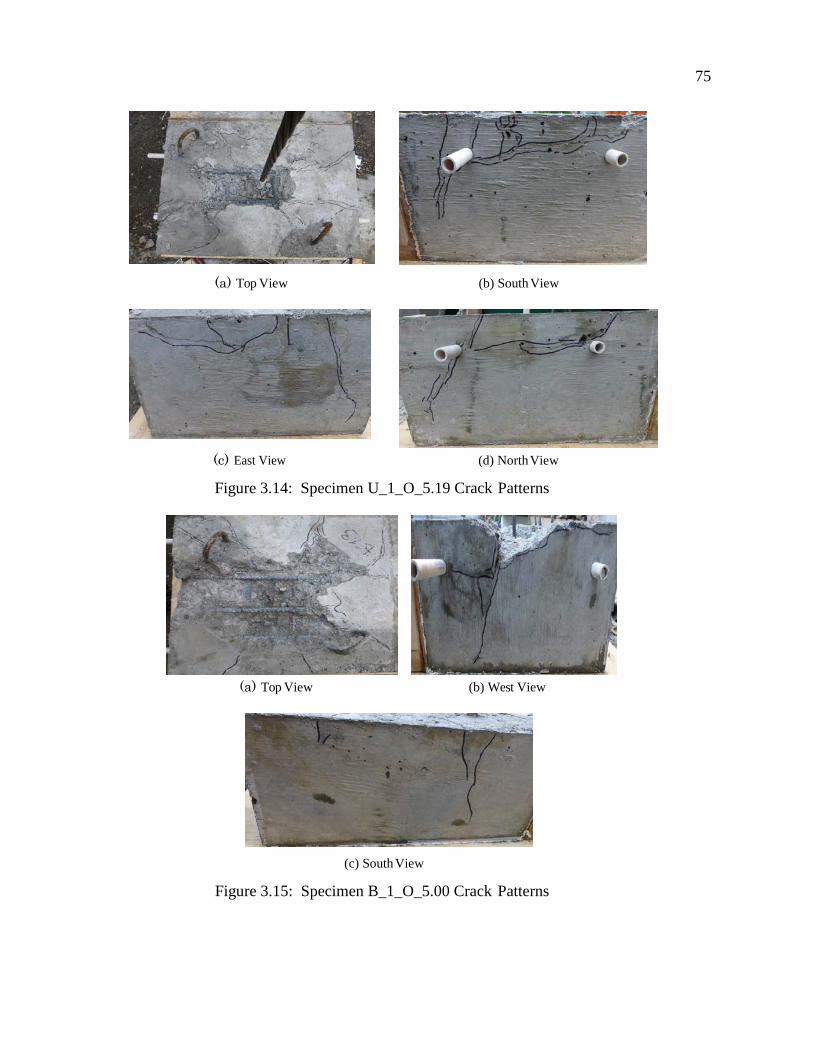
75
(a) Top View (b) South View
(c) East View (d) North View
Figure 3.14: Specimen U_1_O_5.19 Crack Patterns
(a) Top View (b) West View
(c) South View
Figure 3.15: Specimen B_1_O_5.00 Crack Patterns

76 ``
(a) Top View (b) North View
(c) West View (d) South View
Figure 3.16: Specimen U_1_O_6.06 Crack Patterns
(a) Top View (b) South View
(c) West View (d) East View
Figure 3.17: Specimen B_1_4_6.50 Crack Patterns

77
(a) Top View
(b) West View
(c) North View
Figure 3.18: Specimen U_2_L_2.75 Crack Patterns

78 ``
All specimens were designed such that the anchored strands would breakout of the
concrete, creating a conical failure surface. For the specimens with one or two strands, a
breakout failure was observed. However, it was never a pure breakout failure, as one can
see from the photos, since in all cases; the radial cracks propagating from the strand along
the top are often accompanied by some flexural cracks, which in some cases propagate to
the bottom of the specimens.
It should also be noted that in most cases, particularly as depicted in Figures 3.12,
3.16 and 3.18, the compression load generated by the support posts, caused the sides of
the blocks to crack severely, in some cases splitting from the blocks. However, since the
specimen dimensions were chosen such that they would satisfy the required area of
expected breakout cones and the posts were placed on block edges in order to avoid any
interference with the breakout cones, this was thought to have had minimal effects. With
this in mind, looking at the failure cones, the projected breakout area observed on the top
of the blocks matches the predicted area of 3hef x3hef quite closely. Thus, overall, a failure
mode similar to the expected one was achieved.
Photos below show the crack patterns for specimens with four strands.
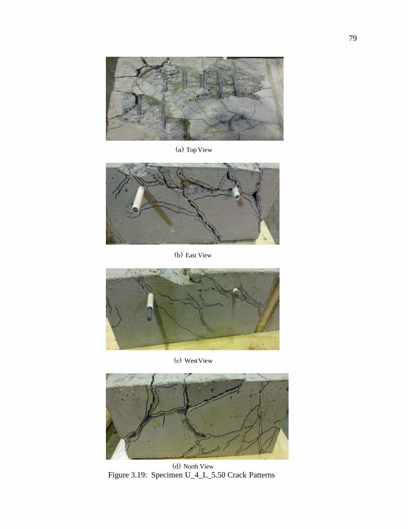
79
(a) Top View
(b) East View
(c) West View
(d) North View
Figure 3.19: Specimen U_4_L_5.50 Crack Patterns

80 ``
As it can be seen in Figure 3.19, severe flexural and shear cracks were observed in specimen
U 4 L 5.50, and the failure mode could be classified as a combination of flexure and shear,
rather than breakout. It should be noted that the radial cracks, accompanying the breakout
cones, observed in all previous (single and two strand) specimens were still present. Severe
cracks under the support posts were present as well.

81
(a) Top View (b) Bottom View
(c) North View (d) South View
(e) East View 1 (f) West View
Figure 3.20: Specimen U_4_L_9.25 Crack Patterns

82 ``
(a) Top View (b) Bottom View
(c) North View (d) South View
(e) East View 1 (f) West View
Figure 3.21: Specimen U_4_S_9.75 Crack Patterns
Specimens U_4_L_9.25 and U_4_S_9.75 exhibit severe shear and flexural cracks but
no radial cracks, propagating from the location of the strands (anchors) can be seen - the
failure mode had fully transitioned from breakout to a combination of bending and shear.

83
Severe flexural cracks can be seen on the bottom, diagonally across the specimen,
underneath where the support HSS posts were placed. The bottom cracks ran
perpendicular to the flexural cracks on the top. This is consistent with the fact that in a
plate subjected to positive bending in one direction, negative moments develop at 90°
to the positive ones. Thus, on the bottom, compressive stresses were acting along the
diagonal underneath the support posts, while tension stresses were generated
perpendicularly to that diagonal, causing the splitting of the concrete. This fact was
overlooked during design, thus no bottom reinforcement was provided. Consequentially,
the bottom cracks could not be inhibited and were quite wide- approximately 1/4 in.

84 ``
(a) Top View (b) Bottom View
(c) North View (d) South View
(e) East View 1 (f) [East View 2
(g) West View
Figure 3.22: Specimen U_4_S_14.5 Crack Patterns

85
For specimen U_4_S_14.5, some flexural cracking can be observed on top of the
specimen, while upon inspection of the sides, some shear cracks propagated down the
sides and along the bottom of the specimen. The bottom view of the specimen shows
concrete splitting, diagonally across the specimen, similarly to what was observed in
specimens U_4_L_9.25 and U_4_S_9.75.
For all cases of groups of strands with higher depth (up to 14.5 in) being tested in
tension, the failure mode switched from breakout to a combination of flexure and shear.
(a) East View
(b) North View (c) Top View
Figure 3.23: Specimen U_4_S_18.5 Crack Patterns
Finally, in the case of the deepest specimen U_4_S_18.5, a maximum load of 231 kips
was achieved and in order to prevent strand fracture, the test was terminated. Thus, it was
concluded that for the given square pattern for four strands, a depth of about 19 in would
be the limit between flexural failure and a ductile failure due to fracture of the strands.
3.6 Analysis of Test Results
This section presents the comparison between test results and the predicted failure loads
from the ACI, PCI and CCD procedures, and discusses the reliability of these models
while deter- mining the required embedment depth of the extended girder strands into
the diaphragm,

86 ``
ensuring ductile failure.
3.6.1 Comparison Between Test Results and CCD, ACI and PCI Methods’ Predictions The specimens were designed according to the procedures described in ACI and PCI in
order to achieve a breakout failure mode for certain target loads.
The failure loads predicted by the Concrete Capacity Design (CCD) method of
analysis were a very close match to the ones obtained from the conducted tests. It should
be noted that the procedures specified in ACI and PCI assume cracked concrete and are
based on the 5% fractile of the database, used to develop the CCD method, while the
CCD approach considers uncracked concrete properties. Thus, the ACI and PCI methods
are more conservative and it was deemed appropriate to match the test data according to
the CCD model, based on the mean values from Eligehausen’s tests for uncracked
concrete specimens, rather than using a 5% fractile and considering cracked concrete.
It should be taken under consideration that a very limited database was used - only 14
tests were conducted - and not in all cases breakout failure was achieved. In specimens
with larger depths the failure occurred due to a combination of flexural and shear
cracking. Yet, the test failure loads match the CCD model almost perfectly in all cases. It
is for this reason that it cannot be claimed with absolute conviction that the CCD
approach will be able to impeccably predict the capacity of a concrete member, regardless
of the edge distance effects, and the anchor groups being investigated.
One thing can be deduced with certainty - the CCD method provides a lower bound to
the true (exact) failure load for these tests. It is for that reason that the obtained results
were deemed sufficient enough that the CCD method was used in estimating the load
capacities for possible strand patterns, extended from the girders into the diaphragm.
Shown below are the failure loads obtained from the tests, as well as the curves
obtained from following the procedures described in ACI, PCI and the CCD
approach. The plots depict the failure loads, normalized with respect to the nominal
strand strength, which was taken as the load, leading to strand fracture, Pfrac = 58 kips
for a single strand for varying block depths and strand patterns.

87
The summary of the tests, carried on specimens with single strands is shown in
Figure 3.24.
Figure 3.24: Normalized Failure Load vs Effective Depth for a Single Strand
Based on the fact that then test results fit the CCD model very closely, it can be
deduced that an embedment depth of 8 in, would be sufficient to ensure a ductile failure
due to strand fracture.
The tests carried out on two strand specimens are summarized in Figure 3.25.

88 ``
Figure 3.25: Normalized Failure Load vs Effective Depth for Two Strands
Considering the fact that the test data seems to fit the CCD model well, it can be
concluded that the required embedment depth for two strands in order to prevent brittle
failure of concrete would be about 11.5 in.
The results for tests, carried out on specimens with four strands in a line are depicted
in Figure 3.26.

89
Figure 3.26: Normalized Failure Load vs Effective Depth for Four Strands in a Line
The test data fits the CCD model very well; thus, it can be deduced that an embedment
depth of 18 in would be sufficient to prevent concrete breakout and provide a ductile
failure mode.
The test results for specimens with four strands in a square pattern are summarized in
Figure 3.27.

90 ``
Figure 3.27: Normalized Failure Load vs Effective Depth- Four Strands in a Block
The test results match the CCD model very closely. Specimen U_4_S_18.50, which was
the deepest specimen tested, did not fail and exhibited no cracking. To prevent strand
fracture, the test was stopped at 231 kips, assuming a nominal strength of 232 kips for
four strands (since Pfrac = 58 kips for a single strand); thus the actual location of the point
representing that specimen would have been higher up on the plot, indicating that the
prediction from the CCD model would likely be slightly smaller than the actual failure
load, similar to all other cases.
The summary of all ultimate test loads normalized with respect to CCD predictions vs
the effective embedment depth is shown in Figure 3.28.

91
Figure 3.28: Normalized Failure Load vs Effective Depth - CCD
As can be seen, the failure loads for the majority of specimens are about 1.1 times the
predicted loads by the CCD method, leading to the conclusion that the Concrete Capacity
Design model is the most reliable one among the three methods described in Section 3.2.
Overall, the failure loads, obtained from experimental data fit the predicted values by
the CCD method much more closely than ACI and PCI predictions. This method was
investigated after the conclusion of the experimental work; thus the design of specimens
was conducted by considering the methodologies described in the subsequent sections
below. The CCD was explored upon the discovery of the conservatism of the ACI and
PCI predictions in comparison with the observed test results.

92 ``
3.6.2 Practical Implications of Breakout Tests The diaphragm region in a typical Washington State bridge bent is very heavily
reinforced, thus, a failure mode, resembling the breakout mechanism, may take place
progressively, rather than suddenly. Since the extended girder strands will be bonded, a
progression of smaller cone failure surfaces would take place along the strand until full
debonding occurred, at which point the strand anchor would bear on the stiff, undamaged
concrete surrounding it, in order to resist the majority of the load. This stage represents
the initiation of the expected 35° breakout failure surface, however its full development
would be arrested by the presence of large amount of flexural and shear reinforcement,
which provide a high degree of confinement. Still, considering how closely the test failure
loads matched those, predicted by the CCD method, it can be used as a guideline in the
determination of the embedment length of the strands into the diaphragm.
3.7 Conclusion
The tests described in this chapter explored the possible failure mechanisms of strands
em- bedded in concrete blocks for different depths and tested in tension. The concrete
block depths were designed according to procedures described in ACI and PCI manuals,
such that a certain target breakout failure load was achieved. Since the test failure loads
were always higher than the design failure loads, the Concrete Capacity Design method,
which is the basis for developing the design methodologies adopted by ACI and PCI, was
investigated and was found to sufficiently correlate to the test ssdata.
Ultimately, since the test results matched the Concrete Capacity Design predictions so
well, it was decided that it can be used to determine the minimum required embedment
depths for different strand patterns to be extended from the girders into the diaphragm in
order to prevent brittle failure due to concrete breakout, ensuring the occurrence of a
ductile failure mode due to fracture of the strands. As a result of these tests, it has been
concluded that using a smaller number of strands embedded in concrete reduces the
likelihood of the occurrence of a brittle breakout failure mode drastically.

93
Chapter 4
DEVELOPMENT OF SUPERSTRUCTURE BRIDGE MODELS 4.1 Introduction
This chapter describes the analyses performed on the bridge superstructure in order to
investigate the system behaviour under the impact of a longitudinal seismic load.
The goals of the analyses were to evaluate the distribution of girder bending
moments across the bridge deck, and to investigate the influence on that distribution of
the most important bridge parameters, such as cracking of bridge components, varying
cross sectional dimensions, and span lengths. If the girder moment distribution is
uniform, the number of strands extended from each girder required to develop the girder-
diaphragm connection could be less than current practice.
The distribution of extended girder strands across the bridge deck depends on the
distribution of girder end moments, which in turn depends on the ratio of the cap beam
torsional stiffness to the girder bending stiffness. If the cap beam is torsionally very stiff,
compared with the flexural stiffness of the girders, the girder moments will be almost
identical, and the same small number of strands could be extended from each girder end
into the diaphragm. Three methods of analysis were pursued to determine the distribution
of bending moments among girders. The issue was investigated by considering a 3-D
model of a typical WSDOT bridge superstructure, followed by the analysis of a less
complicated frame model, and was concluded by creating a continuous model.
4.2 UCSD Tests
Present practice in Washington follows the AASHTO Seismic Design Specifications
(AASHTO, 2009), which is based on tests carried out on two 40%-scale model bridge
structures at UCSD (Holombo et al., 2000).

94 ``
The UCSD tests were based on a typical California cap beam, which is cast-in-place
and flush with the bottom of the girders as shown in Figure 4.1.
(a)
(b)
Figure 4.1: Typical Cap Beams in California Bridges
During the UCSD tests, the cap beam cracked under the effect of torsional moment,
with the result that its stiffness was low, and the majority of the moment imposed by
column bending was resisted by girders within an ”effective width” of the column. The
effective width is defined as the sum of the column diameter and the superstructure
depth, Beff = Dc + Ds, where Dc is the column diameter and Ds is the depth of the
superstructure, including the cap beam, as illustrated in Figure 4.2.
Holombo et al. estimated the contribution of exterior and interior girders to the
resistance of the column plastic moment by considering the distribution of the
longitudinal strains,

95
measured in the deck reinforcement. They concluded that the longitudinal deck strains
recorded over girders within the column effective width were approximately twice as large
as the deck strains recorded over girders outside of the effective width of the column.
Figure 4.2: Effective Superstructure Width (WSDOT, 2015)
4.3 Current Design Practice
Based on the results of the UCSD tests, AASHTO requires that unless an analysis is
carried out to evaluate the stiffness of the girder-bentcap system, it should be assumed
that the girders in close proximity to the column will resist 2/3 of the column plastic
moment and the non-adjacent girders will resist the remaining 1/3.
The design guidelines in the WSDOT Bridge Design Manual (BDM), are based on the
UCSD tests, and include the effective width assumption.
Based on the BDM, for prestressed concrete girders with cast-in-place deck slabs,
where some of the girders are outside the effective widths and the effective widths of the
columns do not overlap, 2/3 of the seismic moment acting at the centroid of the bridge
superstructure will be resisted by girders within the effective width. Thus, the moment
resisted per girder line for girders within the effective width can be calculated as shown
in Equation 4.1.
𝑀𝑀𝑠𝑠𝑏𝑏𝑏𝑏𝐼𝐼𝑏𝑏𝑒𝑒 =
2𝑀𝑀𝑝𝑝𝑛𝑛𝐶𝐶𝐶𝐶
3𝑁𝑁𝑏𝑏𝑏𝑏𝑏𝑏𝑒𝑒 4.1

96 ``
where
𝑀𝑀𝑠𝑠𝑏𝑏𝑏𝑏𝐼𝐼𝑏𝑏𝑒𝑒 is the seismic moment per girder line for girders within the effective width
𝑀𝑀𝑝𝑝𝑛𝑛𝐶𝐶𝐶𝐶 is the plastic hinging moment at the center of gravity of the
superstructure and
𝑁𝑁𝑏𝑏𝑏𝑏𝑏𝑏𝑒𝑒 is the number of girders located within the effective width.
The remainder of the seismic moment, resisted by exterior girders, can be determined
as shown in Equation 4.2.
𝑀𝑀𝑠𝑠𝑏𝑏𝑏𝑏𝐸𝐸𝐸𝐸𝑒𝑒 =
𝑀𝑀𝑝𝑝𝑛𝑛𝐶𝐶𝐶𝐶
3𝑁𝑁𝑏𝑏𝑏𝑏𝐸𝐸𝑒𝑒 4.2
where 𝑀𝑀𝑠𝑠𝑏𝑏𝑏𝑏𝐸𝐸𝐸𝐸𝑒𝑒 is the seismic moment per girderline for girders outside the effective width,
and
𝑁𝑁𝑏𝑏𝑏𝑏𝐸𝐸𝑒𝑒 is the number of girders, outside of the effective width.
Considering Equations 4.1 and 4.2, the seismic moment, Msei, can be determined as
shown in Equation 4.3.
If 𝑀𝑀𝑠𝑠𝑏𝑏𝑏𝑏𝐼𝐼𝑏𝑏𝑒𝑒 ≥ 𝑀𝑀𝑠𝑠𝑏𝑏𝑏𝑏
𝐸𝐸𝐸𝐸𝑒𝑒 𝑀𝑀𝑠𝑠𝑏𝑏𝑏𝑏 = 𝑀𝑀𝑠𝑠𝑏𝑏𝑏𝑏𝐼𝐼𝑏𝑏𝑒𝑒
4.3 If 𝑀𝑀𝑠𝑠𝑏𝑏𝑏𝑏
𝐼𝐼𝑏𝑏𝑒𝑒 < 𝑀𝑀𝑠𝑠𝑏𝑏𝑏𝑏𝐸𝐸𝐸𝐸𝑒𝑒 𝑀𝑀𝑠𝑠𝑏𝑏𝑏𝑏 =
𝑀𝑀𝑝𝑝𝑛𝑛𝐶𝐶𝐶𝐶
𝑁𝑁𝑏𝑏𝑏𝑏𝑏𝑏𝑒𝑒 + 𝑁𝑁𝑏𝑏𝐸𝐸𝐸𝐸𝑒𝑒
This seismic moment is the required moment capacity per girder line (WSDOT, 2015).
Since two girder lines will nearly always be within the column effective width, 𝑀𝑀𝑠𝑠𝑏𝑏𝑏𝑏𝐼𝐼𝑏𝑏𝑒𝑒
would
always be the moment that is considered in the design of all girder lines. This results in a
requirement that all girders be designed for the same end moment, and consequently, the
same number of extended strands.
However, the cap beams in the state of Washington are built in two stages, so the lower
stage can support the precast girders at the time of their erection. They are larger, and
consequently might be expected to lead to a more uniform distribution of girder moments.
If this could be demonstrated, the same total number of extended strands, required to resist
the seismic moment, could be spread over a larger number of girders. Consequently, the

97
maximum number of strands extended from a single girder could be reduced, which
would improve the block pullout strength for a given embedment distance. It would also
reduce the number of bar and strand conflicts that occur during erection. This is
particularly true for curved bridges, for which the opposing girders in a girder line are not
collinear. A reduced number of extended strands would thus provide better
constructability and simpler fabrication through standardization.
4.4 Finite Element 3D Model
ABAQUS software was used to create a 3-D model of a representative WSDOT bridge
and analyze its behaviour under self-weight and longitudinal seismic load.
For the ABAQUS model, the bridge prototype parameters, such as column and cap
beam dimensions, as well as girder type and span lengths, were selected upon examining
the plans of ten typical Washington state bridges. An example of the drawings, showing
the crossbeam detail, is given in Figure 4.3.
Figure 4.3: Prototype Bridge Crossbeam Details
The considerations for the development of the bridge model will be discussed as
follows. First, the configuration of the model, followed by the description of the bridge
components’ geometric

98 ``
and material properties, will be presented. Then, the elements and constraints used in the
finite element model will be examined. Finally, the loading and boundary conditions
applied in the model will be investigated.
The corresponding ABAQUS model is shown in Figure 4.4.
(a) Elevation View (X-Y Plane)
(b) Side View (Z-Y Plane)
Figure 4.4: ABAQUS Model

99
4.4.1 Bridge Prototype The bridge model included a single pier and six WF74G girder lines, supported on a
single- column bent. As previously mentioned, a typical Washington state cap beam
system includes a crossbeam - a lower stage cap - on which girders are erected, and a
diaphragm - an upper stage cap - which is cast after the girder erection, along with the
deck. Consequently, Washington cap beams are much stiffer torsionally, and as a result,
an more uniform girder bending moment distribution is observed, regardless of whether
the column plastic moment is applied to the superstructure at a single point, which is the
case in this model, or if the same total moment is distributed between multiple points, as it
would be for a multi-column bent.
The pier had a circular cross-section with a 6’ diameter and the cap beam cross-section
was idealized as a rectangle. The end of each girder is, in practice, embedded in the cap
beam for a short distance (14.5” for this bridge) as shown in Figure 4.3. However, in the
model, that part of the girder was modeled as if it were a part of the cap beam, and the
higher stiffness of the higher-strength girder concrete started at the outer face of the cap
beam. To model the rest of the bridge superstructure, a composite section, including a
typical WF74G girder cross-section and an 8” thick cast-in-place deck, was used. The
spacing between composite sections was 6’-6” cc. Key dimensions are given in Figure
4.4.
In terms of bridge geometry, the pier had a circular cross-section with a 6’ diameter.
The bent cap cross-section was idealized as a rectangle, excluding the embedment of the
girders into the diaphragm, which is done in practice and shown in Figure 4.3. To model
the rest of the bridge superstructure, a composite section, including a typical WF74G
girder cross-section and an 8” thick cast-in-place deck, was used. The spacing between
composite sections was 6’-6” cc. All dimensions are given in Figure 4.4.
The material properties for each component of the bridge are summarized in Table 4.1.

100 ``
Table 4.1: Bridge Model Material Properties
wE and wDL are the concrete unit weight values, taken from the WSDOT BDM, and
used for the calculation of the modulus of elasticity, and for the calculation of the dead
load, respectively.
The modulus of elasticity, E, for each section was determined as per AASHTO LRFD
Bridge Design Specifications with the expression shown in Equation 4.4 below (AASHTO,
2012).

101
𝐸𝐸 = 33000𝐾𝐾1𝑤𝑤𝐸𝐸1.5�𝑓𝑓 𝑐𝑐′ 4.4
where
K1 = 1.0 is a correction factor for source of aggregate to be taken as 1.0 unless
determined by physical test,
wE is the unit weight of concrete (pcf ), taken according to specifications in WSDOT
BDM,
f’c is the specified compressive strength of concrete (ksi). The resulting values for E for each section are shown in Table 4.1.
4.4.2 Modeling Strategy A linear elastic material model was used to model all bridge components, as the purpose
was to show the general trend of the bridge behaviour under longitudinal seismic load.
The column, cap beam, and composite girders were all modeled as 3-D solid
deformable bodies. The elements used for all components in the ABAQUS model were
C3D8R, that is, continuum (solid), 3-D, 8-node, linear brick (hexahedral) elements with
reduced integration, in order to achieve a less computationally expensive analysis. The cap
beam geometry was simplified as a rectangle in order to facilitate the modeling in
ABAQUS and avoid the use of tetrahedral elements, as the use of the latter may lead to
shear locking, as well as underestimation of displacements and stresses, and is
computationally expensive.
The column-crossbeam and diaphragm-girder surfaces were connected by the use of
tie constraints, which are surface-based constraints, using a master-slave surface
formulation. The ties prevent slave nodes from separating and sliding relative to the
master surface and bond the surfaces permanently. It should be noted that the philosophy
of the tie constraints involves the connection of every node on the master surface to its
closest equivalent, located on the slave surface. This type of constraint accounts for
differences in meshing (different element sizes) in the slave and master surfaces. Models
with and without tie constraints, used to connect the deck portions of the composite
sections to each other were compared to study the influence of a continuous deck on the
overall system behavior.

102 ``
The boundary conditions of the model consisted of pin supports, located at the girder
ends, restricting motion in the x, y and z directions, placed at 52” from the bottom of each
girder, and of pin supports at the bottom of the column surface on two nodes in the X-Z
plane, in the z direction, restricting motion in the y and z directions. The effect of
nonlinear geometry was not considered.
4.4.3 Loading The applied load was estimated from the column flexural strength and length. A 6 ft
diameter column with ρ = 1.55% reinforcement ratio was used in order to determine the
plastic moment capacity, Mp, of the column. No reinforcement was explicitly considered
in the model.
The column dimensions and reinforcement were selected upon investigating a number
of bridges as mentioned earlier.
The column was reinforced with 28#14 bars, thus
𝜌𝜌 =𝐴𝐴𝑠𝑠𝐴𝐴𝑏𝑏
=28(2.25)(4)𝜋𝜋(72)2 4.5
The ratio of the center-to-center distance between the longitudinal reinforcing bars
to the diameter of the column, γ, was determined as follows.
𝛾𝛾 =𝐷𝐷𝑐𝑐 − 2𝑐𝑐𝑐𝑐 − 𝑑𝑑𝑏𝑏 − 2𝑑𝑑𝑏𝑏𝑡𝑡
𝐷𝐷𝑐𝑐 4.6
where Dc is the column diameter (in),
cc is the clear cover (in), chosen to be 1.5”,
db is the diameter of the longitudinal reinforcement (in)
𝑑𝑑𝑏𝑏𝑡𝑡 is the diameter of the transverse reinforcement (in) (here, #9 hoops).
Then,
𝛾𝛾 =72 − 2(1.5) − 1.693 − 2(1.128)
72= 0.903 4.7
Column bending moment-axial force interaction diagram C-5-60-0.9, with γ = 0.9 was used

103
to determine the column moment capacity (Wight and MacGregor 2012). From the diagram,
𝑠𝑠𝑀𝑀𝑏𝑏
𝐴𝐴𝑏𝑏ℎ= 0.51
4.8 𝑠𝑠𝑀𝑀𝑏𝑏 = 0.51 𝐴𝐴𝑏𝑏ℎ
0.9𝑀𝑀𝑏𝑏 = 0.51(𝜋𝜋)(722)(72)
4
𝑀𝑀𝑏𝑏 = 13800 𝑘𝑘 − 𝑓𝑓𝑡𝑡
The plastic moment capacity was then equal to:
𝑀𝑀𝑝𝑝 = 1.2𝑀𝑀𝑏𝑏 = 16600 𝑘𝑘 − 𝑓𝑓𝑡𝑡 4.9
For a column length of 25’ to the inflection point of the load, a longitudinal seismic load
F = 1110 kips was applied to the bottom surface of the column, such that the column
plastic moment would be Mp at the top and zero at the bottom.
4.5 Line Element Model
In order to check the ABAQUS model, a wire frame model was developed, idealizing the
system as a frame structure, using line elements. The stick model is shown in Figure 4.5.
(a) Elevation View (X-Y Plane)
(b) Top View (X-Z Plane)
Figure 4.5: Stick Model

104 ``
The discrete model consists of frame elements, which are deformable in bending
and torsion, with the boundary conditions of the system consisting of a roller
constraint at the bottom end of the column and pin constraints at the remote ends of the
girders. A series of pairs of girders connect to the cap beam at a regular spacing in the
horizontal (X) direction and the column frames into the cap beam at its midpoint from
the bottom in the vertical (Y) direction. Considering the behavior of the system under
longitudinal seismic loading, the torsional rigidity of the cap beam and bending resistance
of the girders govern the overall behavior of the system.
In terms of geometry, the cap beam cross section was idealized as a rectangle, the
column had a circular cross section with a 6’ diameter, and the girders were modeled as
composite WF74G sections with 8” deck on top, similarly to the ABAQUS model. The
system dimensions are shown in Figure 4.5, and the cross sectional properties correspond
to the components shown in Figure 4.4.
The cap beam, column and girders of the real structure were represented as frame
elements located at the centroid of the real elements. To create the frame model, x, y and z
coordinates for the nodes of each element were defined, and element node connectivities
in terms of fixities of the x, y and z axis rotations and displacements were prescribed. A
single-column bent with six girder lines is illustrated in Figure 4.5.
It should be noted that the moment acting at the centroid of the superstructure is
significantly higher than the column plastic moment, Mp. To account for this effect in
the frame model, rigid offset elements, originating from the intersection of the column
centerline and centroid of the composite section and terminating at the sides and bottom
of the cap beam, were added since the frame model represents components as wire
elements through their centerlines. Thus, the girder elements were treated as rigid over a
length 4’ from the centerline of the cap beam, namely, over the half width of the cap
beam. Rigid offset elements, which were 49” wide (girder top flange width) were used
along the cap beam in locations where the girders were connected to it, in order to
account for the fact that the cap beam would be stiffer in locations, where the girders
were framing into it. Similarly, a rigid offset element of 10’-7” was applied at the top of
the column, such that the total torsional moment, acting on the center of gravity of the

105
superstructure would be the same as the ABAQUS model. The rigid offsets are shown
as bold lines in Figure 4.5.
The boundary conditions of the system were the same as the ABAQUS model: the
column was pinned at the bottom, restricting motion in the y and z directions, and the ends
of the girders were pinned, restricting motion in the x, y and z directions, as shown in
4.5a. By using the offset elements as mentioned above, it was ensured that the pin
supports at girder ends were located at 52” from the bottom face of the girders, just as in
the ABAQUS model. No nonlinearities were considered.
A longitudinal load, F = 1110 kips was applied to the bottom of the column, similar
to the ABAQUS model, as shown in 4.5a. This resulted in the same torsional moment
acting at the superstructure center of gravity.
4.6 Continuous Model
As a third analysis strategy, a continuous model of the bridge superstructure was
considered. The cap beam was represented as a line element with torsional stiffness,
and it had rotational springs attached to it, representing the bending stiffness of the girders.
The girder stiffnesses were smeared along the cap beam to create a distributed spring
system. A closed form solution was developed for this system by considering a finite
portion of the cap beam and idealizing it as a rectangular shaft under pure torsion as shown
in Figure 4.6. The effect of gravity was ignored.
Figure 4.6: Continuous Model

106 ``
The continuous model was instrumental in determining the form of the dimensionless
ratios of stiffness and geometry, which governs the distribution of girder moments across
the deck width. The torsional stiffness of the cap beam, GJ, was obtained from its
rectangular cross-section. The girder rotational resistance was represented by a continuous
rotational spring of stiffness per length, β, which can be determined as follows.
𝛽𝛽 =2𝑁𝑁𝐿𝐿𝑃𝑃𝑐𝑐
�3𝐸𝐸𝐼𝐼𝑏𝑏𝑃𝑃𝑏𝑏
� �1
(1 − 𝛼𝛼)3� 4.10
where
NL is the number of girder lines across half the bridge width,
Lc is the length of half of the cap beam (in),
Ig is the moment of inertia of the composite section (WF74G + 8” deck on top) (in4),
Lg is half of the girder span (in)
The factor 2 accounts for the fact that there are two girders per line, and the α accounts for
the rigid end offset in each girder where the girders are attached to the cap beam. It is
given by
𝛼𝛼 = 0.5𝑏𝑏𝑐𝑐𝑏𝑏,𝑏𝑏𝑒𝑒𝑒𝑒
𝑃𝑃𝑏𝑏 4.11
where bcb,eff is the rigid offset along the girders (in), which was taken as 4’, considering the
cap beam width is 8’.
The derivation procedures of the expressions for the distributed spring constant β, as well
as the angle of twist, φ, at any location, z, along the cap beam, are explained below.
If β is the distributed spring constant per unit length, then, the torque applied by
the spring to the cap beam, per unit length, is
𝑡𝑡 = −𝛽𝛽𝑠𝑠 4.12
The resisting torque is
𝑇𝑇 = 𝐺𝐺𝐺𝐺𝑑𝑑𝑠𝑠𝑑𝑑𝑑𝑑
4.13

107
As shown in Figure 4.6, from equilibrium,
𝑑𝑑𝑇𝑇𝑑𝑑𝑑𝑑
+ 𝑡𝑡 = 0 4.14
By combining Equations 4.12 to 4.14, the governing equation for torque is obtained as
follows.
𝐺𝐺𝐺𝐺𝑑𝑑2𝑠𝑠𝑑𝑑𝑑𝑑2
− 𝛽𝛽𝑠𝑠 = 0 4.15
Let
𝜆𝜆2 =𝛽𝛽𝐺𝐺𝐺𝐺
4.16
Then,
𝑑𝑑2𝑠𝑠𝑑𝑑𝑑𝑑2
− 𝜆𝜆2𝑠𝑠 = 0 4.17
The solution has the following form
𝑠𝑠(𝑑𝑑) = 𝐴𝐴𝑒𝑒𝜆𝜆𝑧𝑧 + 𝐵𝐵𝑒𝑒−𝜆𝜆𝑧𝑧 4.18
which can equivalently be represented as
𝑠𝑠(𝑑𝑑) = 𝐴𝐴𝑐𝑐𝐴𝐴𝑠𝑠ℎ(𝜆𝜆𝑑𝑑) + 𝐵𝐵𝑠𝑠𝑠𝑠𝑠𝑠ℎ(𝜆𝜆𝑑𝑑) 4.19
Substituting Equation 4.19 into Equation 4.13 gives the torque
𝑇𝑇(𝑑𝑑) = 𝐺𝐺𝐺𝐺𝜆𝜆[𝐴𝐴𝑠𝑠𝑠𝑠𝑠𝑠ℎ(𝜆𝜆𝑑𝑑) + 𝐵𝐵𝑐𝑐𝐴𝐴𝑠𝑠ℎ(𝜆𝜆𝑑𝑑)] 4.20
If we consider half of the cap beam, with length Lc, the torsional moment To, acting on
the cap beam end, originates as a bending moment in the column, when the bridge is
subjected to horizontal load. Then, this bending moment is transferred from the column
to the cap beam as torsional moment. The magnitude of To is half of the plastic hinging
moment acting on the center of gravity of the superstructure.
At z = Lc, namely, at the outer end of the cap beam, there is no torque acting on the cap
beam; hence,

108
``
𝑇𝑇(𝑃𝑃𝑐𝑐) = 0 = 𝐺𝐺𝐺𝐺𝜆𝜆𝐴𝐴[𝑠𝑠𝑠𝑠𝑠𝑠ℎ(𝜆𝜆𝑃𝑃𝑐𝑐) + 𝐵𝐵𝑐𝑐𝐴𝐴𝑠𝑠ℎ(𝜆𝜆𝑃𝑃𝑐𝑐)] 4.21
Adjacent to the column, at z = 0, the torque To is acting on the cap beam; hence,
𝑇𝑇(0) = 𝑇𝑇𝑛𝑛 = 𝐺𝐺𝐺𝐺𝜆𝜆𝐴𝐴[𝑠𝑠𝑠𝑠𝑠𝑠ℎ(0) + 𝐵𝐵𝑐𝑐𝐴𝐴𝑠𝑠ℎ(0)] = 𝐺𝐺𝐺𝐺𝜆𝜆𝐵𝐵 4.22
As a result,
𝐵𝐵 =𝑇𝑇𝑛𝑛𝐺𝐺𝐺𝐺𝜆𝜆
4.23
From Equation 4.21,
𝐴𝐴 = −𝑇𝑇𝑛𝑛𝐺𝐺𝐺𝐺𝜆𝜆
𝑐𝑐𝐴𝐴𝑡𝑡ℎ( 𝜆𝜆𝑃𝑃𝑐𝑐) 4.24
Thus,
𝑇𝑇(𝑑𝑑) = −𝑇𝑇𝑛𝑛 𝑐𝑐𝐴𝐴𝑡𝑡ℎ( 𝜆𝜆𝑃𝑃𝑐𝑐) 𝑠𝑠𝑠𝑠𝑠𝑠ℎ(𝜆𝜆𝑑𝑑) + 𝑇𝑇𝑛𝑛 𝑐𝑐𝐴𝐴𝑠𝑠ℎ(𝜆𝜆𝑑𝑑) 4.25
And from Equation 4.19,
𝑠𝑠(𝑑𝑑) = −𝑇𝑇𝑛𝑛𝐺𝐺𝐺𝐺𝜆𝜆
𝑐𝑐𝐴𝐴𝑠𝑠ℎ(𝜆𝜆𝑃𝑃𝑐𝑐)𝑠𝑠𝑠𝑠𝑠𝑠ℎ(𝜆𝜆𝑃𝑃𝑐𝑐) 𝑐𝑐𝐴𝐴𝑠𝑠ℎ
(𝜆𝜆𝑑𝑑) +𝑇𝑇𝑛𝑛𝐺𝐺𝐺𝐺𝜆𝜆
𝑠𝑠𝑠𝑠𝑠𝑠ℎ(𝜆𝜆𝑑𝑑)
4.26
𝑠𝑠(𝑑𝑑) =𝑇𝑇𝑛𝑛𝐺𝐺𝐺𝐺𝜆𝜆
�−𝑐𝑐𝐴𝐴𝑠𝑠ℎ(𝜆𝜆𝑃𝑃𝑐𝑐) 𝑐𝑐𝐴𝐴𝑠𝑠ℎ(𝜆𝜆𝑑𝑑) + 𝑠𝑠𝑠𝑠𝑠𝑠ℎ(𝜆𝜆𝑃𝑃𝑐𝑐) 𝑠𝑠𝑠𝑠𝑠𝑠ℎ(𝜆𝜆𝑑𝑑)
sinh(𝜆𝜆𝑃𝑃𝑐𝑐) �
𝑠𝑠(𝑑𝑑) =𝑇𝑇𝑛𝑛𝐺𝐺𝐺𝐺𝜆𝜆
�𝑐𝑐𝐴𝐴𝑠𝑠ℎ(𝜆𝜆(𝑃𝑃𝑐𝑐 − 𝑑𝑑))
sinh(𝜆𝜆𝑃𝑃𝑐𝑐) �
Similarly, from Equation 4.20,
𝑇𝑇(𝑑𝑑) = 𝑇𝑇𝑛𝑛 �𝑠𝑠𝑠𝑠𝑠𝑠ℎ(𝜆𝜆(𝑃𝑃𝑐𝑐 − 𝑑𝑑))
sinh(𝜆𝜆𝑃𝑃𝑐𝑐) � 4.27
For the reference bridge model, λLc = 0.435.

109
The distribution of torque along the cap beam is illustrated in Figure 4.7.
Figure 4.7: Torsional Moment Distribution Along Cap Beam
The torque distribution along the cap beam is shown for two different values of
λLc; λLc = 0.435 for the reference structure, and λLc = 1.947 for a structure, which has a
smaller cap beam, which would have a much smaller torsional stiffness. The torsional
moment distribution is much less uniform for a structure with low cap beam torsional
stiffness.
The real structure consists of discrete girders and not a continuous rotational spring.
Thus, the structure can be discretized to include a number of rotational springs,
representing the girders, and as that number of girders approaches infinity, the model
would behave as the continuous system, since the infinite number of springs would be
equivalent to the girders being smeared along the cap beam.

110
``
The moment attributable to each girder can be obtained as the change in torque in the cap
beam from one side of the girder to the other. For girder line i, the relevant z values are
𝑑𝑑𝑏𝑏 = 𝑃𝑃𝑐𝑐 − 𝑠𝑠𝑠𝑠𝑏𝑏 4.28
and
𝑑𝑑𝑏𝑏−1 = 𝑃𝑃𝑐𝑐 − (𝑠𝑠 − 1)𝑠𝑠𝑏𝑏 4.29
where the girder spacing, 𝑠𝑠𝑏𝑏 = 𝐿𝐿𝑐𝑐𝑁𝑁𝐿𝐿
, and NL is the number of girder lines along (half of
the) cap beam length Lc as shown in Figure 4.8. Note that the structure shown here is
the prototype bridge and it includes three girder lines.
Figure 4.8: Discretization of Continuous Model
Thus, the moment in a single girder on line i is given by
𝑀𝑀𝑏𝑏,𝑏𝑏 =12
𝑇𝑇𝑛𝑛𝑠𝑠𝑠𝑠𝑠𝑠ℎ(𝜆𝜆𝑃𝑃𝑐𝑐) �sinh �𝜆𝜆𝑃𝑃𝑐𝑐 �1−
𝑠𝑠 − 1𝑁𝑁𝐿𝐿
�� − sinh �𝜆𝜆𝑃𝑃𝑐𝑐 �1−𝑠𝑠𝑁𝑁𝐿𝐿��� 4.30
where the factor 1/2 accounts for the fact that two girders per line are framing into the cap
beam Upon the application of several sum and difference of angle formulas for hyperbolic
functions, Equation 4.30 can be further simplified to
𝑀𝑀𝑏𝑏,𝑏𝑏 = 𝑇𝑇𝑛𝑛𝑠𝑠𝑠𝑠𝑠𝑠ℎ �𝜆𝜆𝑃𝑃𝑐𝑐2𝑁𝑁𝐿𝐿
�
𝑠𝑠𝑠𝑠𝑠𝑠ℎ(𝜆𝜆𝑃𝑃𝑐𝑐) 𝑐𝑐𝐴𝐴𝑠𝑠ℎ � 𝜆𝜆𝑃𝑃𝑐𝑐 �1−𝑠𝑠 − 1/2𝑁𝑁𝐿𝐿
�� 4.31

111
The largest cap beam torque takes place in the regions closest to the column, hence the
girder lines, located in the closest proximity to the column will exhibit the largest bending
moments as shown in Figure 4.9.
Figure 4.9: Girder Moment Distribution Along Cap Beam
It should be noted that the ratio of the maximum girder moment, Mg,max to the average
girder moments, Mg,avg , was selected as an appropriate normalization in order to depict the
change in the bending moments in the girders along the cap beam, or with varying girder
stiffnesses and number of girders.
The average moment across the NL girder lines is

112 ``
𝑀𝑀𝑏𝑏,𝑏𝑏𝑎𝑎𝑏𝑏 =𝑇𝑇𝑛𝑛
2𝑁𝑁𝐿𝐿 4.32
For the girder lines closest to the column, i = 1, so the ratio 𝑀𝑀𝑔𝑔,𝑚𝑚𝑚𝑚𝑚𝑚
𝑀𝑀𝑔𝑔,𝑚𝑚𝑎𝑎𝑔𝑔 is
𝑀𝑀𝑏𝑏,𝑚𝑚𝑏𝑏𝐸𝐸
𝑀𝑀𝑏𝑏,𝑏𝑏𝑎𝑎𝑏𝑏= 2𝑁𝑁𝐿𝐿
𝑠𝑠𝑠𝑠𝑠𝑠ℎ �𝜆𝜆𝑃𝑃𝑐𝑐2𝑁𝑁𝐿𝐿�
𝑠𝑠𝑠𝑠𝑠𝑠ℎ(𝜆𝜆𝑃𝑃𝑐𝑐) 𝑐𝑐𝐴𝐴𝑠𝑠ℎ �λLc �1 −1
2NL�� 4.33
This development shows that the distribution of girder moments is controlled by the
dimensionless parameters λLc, and NL. λLc is the square root of the ratio of the flexural
stiffness of the girders to the torsional stiffness of the cap beam.
𝜆𝜆𝑃𝑃𝑐𝑐 = �𝛽𝛽𝑃𝑃𝑐𝑐2 𝐺𝐺𝑐𝑐𝐺𝐺𝑐𝑐
4.34 𝜆𝜆𝑃𝑃𝑐𝑐 = �(𝐾𝐾𝑏𝑏/𝑃𝑃𝑐𝑐)𝑃𝑃𝑐𝑐2
𝐺𝐺𝑐𝑐𝐺𝐺𝑐𝑐
𝜆𝜆𝑃𝑃𝑐𝑐 = �𝐾𝐾𝑏𝑏 𝐾𝐾𝑐𝑐
where
𝐾𝐾𝑏𝑏 = 2(𝑁𝑁𝐿𝐿)3𝐸𝐸𝑏𝑏𝐼𝐼𝑏𝑏
𝑃𝑃𝑏𝑏(1− 𝛼𝛼3) 4.35
which is the total flexural stiffness of all of the girders within half of the bridge width, and
𝐾𝐾𝑐𝑐 =𝐺𝐺𝐶𝐶𝐺𝐺𝑐𝑐𝑃𝑃𝑐𝑐
4.36
which is the torsional stiffness of half of the cap beam.
Since the cap beam would be torsionally stiffened where the girders are connecting to
it, a modification to increase the cap beam stiffness was deemed necessary. The torsional
stiffness of the cap beam was increased by increasing Gc rather than decreasing the free
length between girders. The factor used was cG, where

113
𝑐𝑐𝐶𝐶 =𝑠𝑠𝑏𝑏
𝑠𝑠𝑏𝑏 − 𝑏𝑏𝑏𝑏,𝑏𝑏𝑒𝑒𝑒𝑒 4.37
where bg,eff is the rigid element offset along the cap beam, taken as 49” for the reference
structure.
Thus, the finalized expression for λLc would be
𝜆𝜆𝑃𝑃𝑐𝑐 = �(2𝑁𝑁𝐿𝐿)3𝐸𝐸𝑏𝑏𝐼𝐼𝑏𝑏 𝑃𝑃𝑐𝑐
𝐺𝐺𝑐𝑐𝑐𝑐𝐶𝐶𝐺𝐺𝑐𝑐𝑃𝑃𝑏𝑏(1− 𝛼𝛼3) 4.38

114 ``
Chapter 5
SUPERSTRUCTURE ANALYSIS RESULTS AND DISCUSSION
5.1 Introduction
A parametric study was conducted in order to investigate the effects of varying some of
the important parameters in the models (ABAQUS Model, Stick Model, and Continuous
Model). First, the structure was investigated under uncracked elastic conditions, and the
effects of changing the member stiffness, global geometry, and numbers of girders were
studied. Then the effects of concrete cracking and strand yielding were investigated.
Finally, the results of the parameter study were correlated, and were compared with
Priestley and Holombo’s recommendations.
5.2 Elastic Uncracked Sections - Effect of Rigid-End Offsets (REO)
A bridge bent with six girder lines across the full bridge width, was used as a reference
structure in order to compare the behaviour, predicted by the different models.
The part of the structure for which girder moment distributions will be evaluated, as
well as the girder line numbering, are depicted in Figure 5.1.
Figure 5.1: ABAQUS Model Top View (X-Z Plane) and Girder Numbers

115
5.2.1 Calibration Between Models A single ABAQUS model was used to determine the girder moments for the reference
structure. All bridge components were solid elements, and thus there was no need for rigid
end offsets, used in the other two models. As the joint region is not completely stiff, the
lengths of the rigid end offsets are expected to not be exactly equal to the widths of the
cap beam and girder sections.
The stick and ABAQUS models were run with uncracked elastic material properties,
and the rigid end offsets in the stick model were adjusted as follows. The girders were
treated as 49” wide, and the cap beam was treated as torsionally rigid within that width.
Realistically, since only the girder top flanges are 49” wide, the true width, over which the
cap beam should be considered torsionally rigid, is actually less than 49”. Thus, to check
the effect of the girder width, portions of the cap beam between girders, which are
torsionally flexible, were considered as both the full 78”, which was the center to center
spacing between girders, and 29”, which would be the clear spacing between girders. It
was deemed sufficient to check these two most extreme cases, with the prior being the
worst case scenario, where essentially the girders provide no torsional rigidity to the cap
beam, and the latter being the best case scenario, where the girders provide maximum
torsional rigidity to the cap beam.
The continuous model matched the other two models when rigid end offsets for full
width of the cap beam and girder sections were used.
Considering elastic uncracked section properties for all bridge components, the
distribution of girder moments is shown for all three models for the reference structure in
Figure 5.2.

116 ``
Figure 5.2: Girder Moment Distribution Along Half Cap Beam, Full Width REO This plot depicts the moment distribution in terms of the girder bending moment, normalized
with respect to the average moment in all girders (a total of 3 girder lines), considering half of
the bridge superstructure. All three models agree in terms of the general trend regarding the
girder bending moment distribution, namely, that the girder moments are almost uniformly
distributed, with highest magnitudes closest to the pier. This distribution is expected, since the
largest torsional moment in the cap beam is located in the middle of the cap beam and that
moment magnitude gets smaller with distance farther and farther from mid-cap beam. The
cap beam would transfer that torsional moment as a bending moment to the girders, and the
largest bending moments would occur in girders closest to the column, which is the case
here. The maximum girder moment is less than 4% larger than the average moment. The
Stick Model and the Continuous Model give almost identical results, whereas the ABAQUS
model deviates slightly. However, it should be noted that the ABAQUS model values vary
within less than 0.6% from the other models. Thus, the results are deemed acceptable.

117
Furthermore, the results depicted here include the full width rigid end offsets (REO),
namely, 48” along each girder, and 49” along the cap beam, wherever girders are connected
to it, for both the Continuous and Stick models.
Figure 5.3: Girder Moment Distribution Along Half Cap Beam REO Impact
To check the effect of the rigid offsets, results for the Stick and Continuous Models
without including any offsets were compared with the previously shown results for all
models, which included the rigid offsets. As it can be seen, the girder moment distribution
is less uniform when rigid end offsets are ignored. This is to be expected as ignoring the
rigid end offsets assumes the cap beam is less torsionally stiff than it would be in reality. It
was discovered that the difference in girder moments was less than 5% between stick
models (or continuous models since they behave the same) when rigid end offsets were
accounted for and when their effect was excluded.

118 ``
5.3 Elastic Uncracked Sections - Effect of Stiffness Ratio The distribution of moments among the girders depends on the relative stiffnesses of the girder
and cap beam. The two parameters that determine girder bending moment distribution are λLc
and NL, which are defined in Section 4.6. It is convenient to separate these two parameters, such
that the total girder stiffness Kg = 2(NL)3EgIgLg(1−α)3 would always be kept the same by reducing EgIg
for increasing NL. That way, considering Equation 4.33, one would be able to observe the
variation in moment distribution for a constant number of girder lines, NL, and varying λLc
values. In a similar manner, when the distribution of moments with varying NL is investigated, it
would be ensured that λLc stays constant. The effects of changing the relative stiffnesses
between the girders and cap beam, namely by varying λLc, were studied using the geometry of
the reference structure (three girder lines in the half width of the deck), and rigid-end offsets
equal to the full beam width. The stiffness of the girders was varied from 0.069 to 20 times their
reference value. The lower limit was selected based on the bending stiffness of a cracked
WF74G girder, which would be approximately 6.9% of its uncracked stiffness. The upper limit,
20, represents the ratio of girder bending to cap beam torsional stiffnesses which would take
place if the cap beam were to crack completely, resulting in it having a torsional stiffness equal
to 5% of its uncracked value. The λLc value will change either due to a variation in the cross-
sectional dimensions of the girders and/or the cap beam, or due to cracking. The effect of the
latter will be discussed later in more detail. For reference, λLc = 0.435 is the value for the
reference structure for uncracked elastic section properties and the corresponding moment
ratio 𝑀𝑀𝑔𝑔,max
𝑀𝑀𝑔𝑔,𝑚𝑚𝑎𝑎𝑔𝑔 is 1.040 for the ABAQUS model and 1.035 for the Stick and Continuous models.
The ratio 𝑀𝑀𝑔𝑔,max
𝑀𝑀𝑔𝑔,𝑚𝑚𝑎𝑎𝑔𝑔 is plotted against λLc in Figure 5.4.

119
Figure 5.4: Girder Moment Distribution with Varying Stiffness Ratio, Full REO, NL = 3
The plot shows that the ratio 𝑀𝑀𝑔𝑔,max
𝑀𝑀𝑔𝑔,𝑚𝑚𝑎𝑎𝑔𝑔 increases with λLc, that is, as the girder bending
stiffness increases relative to the torsional stiffness of the cap beam.
The ABAQUS model is a more complicated finite element model, compared to the
stick model, and some of the 3-D solid element interaction might be causing the
observed trend, since the girder moments, obtained from ABAQUS are more uniformly
distributed compared to the other models. However, at low values of λLc the ABAQUS
model approaches the exact solution and follows the trend of the other models.
All in all, the expected system behaviour is similar for all three models.
5.4 Elastic Uncracked Sections - Effect of Number of Girders The effect of the second parameter, namely number of girder lines, NL, on the girder
moment distribution, is complicated by consideration of the rigid-end offsets. If the cap

120 ``
beam length had been kept constant, while the number of girders increased, the space
between girders would diminish and the cap beam would become stiffer in torsion,
thereby changing λLc. If rigid end offsets were accounted for, the cap beam would
become torsionally stiffer, making the distribution of girder moments more uniform. The
extent to which this happens depends on the size of the rigid end offset. Thus, that feature
of modeling affects the influence of the number of girders. Ergo, to investigate the effect
of changing the number of girder lines, the rigid end offsets in the stick and continuous
models were ignored and the stiffness ratio λLc = 0.681 was used in all cases. Note that
λLc = 0.435 until now for uncracked section properties, because full width rigid end
offsets were used. λLc = 0.681 is the stiffness ratio, corresponding to uncracked section
properties, considering a model with no rigid offsets.
The stick model was developed for a superstructure with a maximum of 8 girder lines along
half of the bridge width, in order to see the pattern in girder moment distribution for a large
number of small girders. The number of girders in the half width of the bridge was limited to 8,
because this is likely to be an upper bound to the number of girders used in practice. The cap
beam length and the total girder stiffness were kept at the same as in the reference structure, and
the number of girders and their individual stiffnesses were varied. The results are shown in
Figure 5.5.

121
(a) 3 Girder Lines
(b) 8 Girder Lines
Figure 5.5: Girder Moment Distribution vs Number of Girder Lines, No REO, λLc = 0.681

122 ``
The use of more and smaller girders leads to maximum girder moments that are higher
proportions of the average.
Equation 5.1, which predicts the maximum girder moment using the continuous
model as a function of the number of girders, can be used to find 𝑀𝑀𝑔𝑔,𝑚𝑚𝑚𝑚𝑚𝑚
𝑀𝑀𝑔𝑔,𝑚𝑚𝑎𝑎𝑔𝑔 as NL approaches
infinity. The limit is
𝑀𝑀𝑏𝑏,𝑚𝑚𝑏𝑏𝐸𝐸
𝑀𝑀𝑏𝑏,𝑏𝑏𝑎𝑎𝑏𝑏= 2𝑁𝑁𝐿𝐿
�𝜆𝜆𝑃𝑃𝑐𝑐2𝑁𝑁𝐿𝐿 �
𝑡𝑡𝑡𝑡𝑠𝑠ℎ (𝜆𝜆𝑃𝑃𝑐𝑐)=
𝜆𝜆𝑃𝑃𝑐𝑐𝑡𝑡𝑡𝑡𝑠𝑠ℎ(𝜆𝜆𝑃𝑃𝑐𝑐) 5.1
As λLc increases, 𝑀𝑀𝑔𝑔,𝑚𝑚𝑚𝑚𝑚𝑚
𝑀𝑀𝑔𝑔,𝑚𝑚𝑎𝑎𝑔𝑔 approaches λLc.
Figure 5.6: Girder Moment Distribution with Varying Stiffness Ratio for Different
Number of Girder Lines, No REO

123
Figure 5.5 shows results for a single λLc value and variable number girder lines, NL. The
change in 𝑀𝑀𝑔𝑔,𝑚𝑚𝑚𝑚𝑚𝑚
𝑀𝑀𝑔𝑔,𝑚𝑚𝑎𝑎𝑔𝑔 for several NL and variable λLc values is illustrated in Figure 5.6. It shows that,
for large enough λLc, the moment ratio is asymptotic to NL. This implies that all the moment is
resisted by the first line of girders, which is what is to be expected when the girders are very stiff
relative to the cap beam. This can also be shown mathematically, because for very large λLc,
looking back at Equation 4.33, an indeterminate form ∞∞ is observed and by using L’Hospital’s
Rule, Equation 4.33 approaches
𝑀𝑀𝑏𝑏,𝑚𝑚𝑏𝑏𝐸𝐸
𝑀𝑀𝑏𝑏,𝑏𝑏𝑎𝑎𝑏𝑏= 𝑁𝑁𝐿𝐿 5.2
Figure 5.7: Girder Moment Distribution with Varying Stiffness Ratio for Different Number of Girder Lines, No REO

124 ``
This finding shows that the continuous model gives appropriate results at the extremes, but
the λLc values required to achieve this result are much higher than the ones likely to occur in
practice. The girder moment distribution for various numbers of girder lines and for a
restricted and more practical range of λLc values is shown in Figure 5.7.
As it can be seen in Figure 5.6 and Figure 5.7, the girder moments distribution is less
and less uniform for a larger number of girders for the same λLc value. As NL becomes
large, the maximum girder moment approaches the limiting value λLc, and suggests that
normalization by Mg,avg may be useful when the number of girders is small, but less so
when many small girders are used. In case of the latter, normalization by half of the
torsional moment acting on the centroid of the superstructure, To, may be more useful.
However, for the current normalization, it should be noted that as λLc becomes very large,
i.e. when the girders are much stiffer than the cap beam, the ratio 𝑀𝑀𝑔𝑔,max
𝑀𝑀𝑔𝑔,𝑚𝑚𝑎𝑎𝑔𝑔 converges to the
number of girder lines (along half the width of the bridge), NL.
5.5 Effect of Cracking
When a vertical crack forms at the end of the girder (at the girder-diaphragm interface)
and the extended strands start to work, the girder stiffness will be reduced significantly; it
would be approximately 6.9% of its uncracked value for a girder with 10 extended
strands. The (fully) cracked cap beam torsional stiffness was assumed to be 5% of its
uncracked stiffness, as advised in (Priestley et al., 1996).
To observe the effect of varying girder to cap beam stiffness ratios on the girder
moment distribution, several cases were investigated. Progressively decreasing girder
stiffnesses, ranging between 100% (uncracked) and 6.9% (fully cracked) were considered
separately from progressively decreasing cap beam stiffnesses, ranging between 100% and
5%. The changes to the stiffnesses were applied by changing the modulus of elasticity, E,
for each bridge com- ponent. Finally, a case, in which both the cap beam and the girders to
be fully cracked, was considered.
The effect of the cracking of the cap beam and girders separately and together on the

125
uniformity of girder moments is illustrated in Figure 5.8 for the ABAQUS Model
results, considering the reference structure. As the other models agree closely with the
ABAQUS one, their results are not shown.
Figure 5.8: Variation in Girder Moment Ratio Along Cap Beam for the Effect of Component Cracking
If only the girders are fully cracked, then all girder moments will be almost identical
and the most uniform girder moment distribution is observed.
The effect of severe cracking of the cap beam with little to no cracking in the girders
leads to the most non-uniform distribution of girder moments. In such a case, much larger
moments are acting on girders in close proximity to the pier (within its effective width)
and much smaller moments act on the edge girders.
Finally, the girder moment distribution is almost equivalent (and fairly uniform) in

126 ``
the cases where nothing is cracked and when both the cap beam and girders are fully
cracked. The same trend can be observed from Figure 5.4; namely, that for small values
of λLc, which would represent a small ratio of the girder bending stiffness to the cap beam
torsional stiffness, the moment distribution between girders is almost uniform.
Similarly, for large values of λLc, which represent a low ratio of the girder to cap beam
stiffness and would occur when only the cap beam was cracked, the girder moment
distribution is less and less uniform. Presumably, in reality, the highest 𝑀𝑀𝑔𝑔,𝑚𝑚𝑚𝑚𝑚𝑚
𝑀𝑀𝑔𝑔,𝑚𝑚𝑎𝑎𝑔𝑔 ratio would
be observed for a completely cracked cap beam and uncracked girders. Theoretically, the
largest value of 𝑀𝑀𝑔𝑔,𝑚𝑚𝑚𝑚𝑚𝑚
𝑀𝑀𝑔𝑔,𝑚𝑚𝑎𝑎𝑔𝑔 would be the number of girder lines, NL. This is unlikely to be
observed in reality, as the value of λLc needs to be very large, namely at least 60 for 3 girder
lines (the reference structure) in order for 𝑀𝑀𝑔𝑔,𝑚𝑚𝑚𝑚𝑚𝑚
𝑀𝑀𝑔𝑔,𝑚𝑚𝑎𝑎𝑔𝑔 to converge to NL = 3. That means the
total girder bending stiffness to cap beam torsional stiffness ratio needs to be 3600, which is
deemed unlikely. For reference, if the cap beam is completely cracked (down to 5% of its
uncracked stiffness), λLc is less than 2, including rigid offsets. Excluding the latter, λLc was
determined to be around 3.
Finally, if the strands extended from the girders are yielding, this would be equivalent
to considering the variation in moments for a low value of λLc, thus leading to a more
uniform girder moment distribution.
Looking at the girder moment variations in all models, it could be concluded that
the results of the UCSD tests involved a system with a torsionally very weak cap beam
(even though it was PT), which cracked extensively, while the girders remained
almost at full capacity (that is what their moment distribution, as well as photos of the
post-test suggest), thus leading to the conclusion of 2/3 - 1/3 moment distribution.
5.6 Likelihood of Cracking For all the models discussed, the effect of cracking was considered by progressively
increasing the degree of cracking in the cap beam and the girders, both individually and
concurrently. This section discusses the likelihood and extent of cracking of these
components.

127
5.6.1 Cap Beam Cracking
The shear stresses in the cap beam caused by the torsional moment, acting at the center of gravity
of the superstructure, were investigated in the ABAQUS model with uncracked section
properties. The maximum shear stress in the cap beam at Z = 78 in., namely the location
between girder lines 1 and 2, shown in Figure 5.1, was τmax = 390 psi and it was observed at the
mid-bottom of the cap beam. The cap beam concrete, which uses the WSDOT 4000D mix,
almost always has strength greater than 5000 psi. At the time of the earthquake, it is likely to be
stronger still. If the cracking limit in shear is considered to be 4�𝑓𝑓 𝑐𝑐′ for the cap beam this limit
would be equal to 282 psi, considering an f’ c= 5000 psi. c c
The portion of the structure where the shear stresses were checked is shown in Figure 5.9.
Figure 5.9: Cap Beam Location for Shear Stresses
The shear stresses in the cap beam between girder lines 1 and 2, namely at Z=78”, are
shown in Figure 5.10.

128 ``
(a) Shear Stress, τxz vs Horizontal Location
(b) Shear Stress, τyz vs Vertical Location
Figure 5.10: Cap Beam Shear Stress vs Location, Z=78”

129
Thus, the cap beam should be expected to crack adjacent to the column as it
experiences shear stresses exceeding the cracking limit. The shear stresses in the cap beam
between girder lines 2 and 3 were lower than or barely approaching the cracking limit of
282 psi. Therefore, the cap beam will not crack there.
These results were checked against the Stick model maximum shear stress as follows.
The shear stress in a rectangular section, caused by a torsional moment can be
determined by
𝜏𝜏𝑀𝑀𝑡𝑡 =𝑀𝑀𝑒𝑒
𝛽𝛽𝑠𝑠𝑏𝑏𝑐𝑐𝑡𝑡𝑐𝑐2 5.3
where Mt is the torsional moment acting on the section, taken as the torsional moment acting on
the superstructure between girder lines 1 and 2, namely Mt = 109500 k − in
bc = 149 in is the larger dimension and tc = 96 in. is the smaller dimension of the
cap beam, βs is a dimensionless coefficient, and it is determined by Equation 5.4
(Stanton, 2002)
𝛽𝛽𝑠𝑠 = 1
3[0.742454 + 𝑡𝑡𝑐𝑐𝑏𝑏𝑐𝑐
(0.5 + 0.375 𝑡𝑡𝑐𝑐𝑏𝑏𝑐𝑐)]
5.4
𝛽𝛽𝑠𝑠 = 0.273
Note that typically in a rectangular section, the maximum shear stress would be
observed in the middle of the long side of the section. However, this is expected to occur
under the impact of pure torsion. Here, there are also shear forces acting on the cap beam,
both from the girders and the column. Upon investigation, it was determined that the total
shear force applied by the girders is much smaller, when compared to the column shear
force. Thus, the maximum shear stress, observed in the cap beam would occur in its mid-
bottom, where the effects of torsional moment and column shear force coincide. This can
also be seen from the ABAQUS results in Figure 5.10.

130 ``
𝜏𝜏𝑀𝑀𝑡𝑡 =109500
(0.273)(149)(96)2 5.5
𝜏𝜏𝑀𝑀𝑡𝑡 = 0.292 𝑘𝑘𝑠𝑠𝑠𝑠
The maximum transverse shear stress caused by the impact of a shear force can be
determined as shown in Equation 5.6
𝜏𝜏𝑉𝑉,𝑚𝑚𝑏𝑏𝐸𝐸 =32𝑉𝑉𝑐𝑐𝐴𝐴𝑐𝑐
5.6
where
Vc is the shear force acting on half of the cap beam from the column, Vc = 555 kips,
Ac is the cross-sectional area of the cap beam, calculated as follows
𝐴𝐴𝑐𝑐 = 𝑏𝑏𝑐𝑐𝑡𝑡𝑐𝑐
5.7 𝐴𝐴𝑐𝑐 = 149(96)
𝐴𝐴𝑐𝑐 = 14300 𝑠𝑠𝑠𝑠2
Thus,
𝜏𝜏𝑉𝑉,𝑚𝑚𝑏𝑏𝐸𝐸 =32
55514300
5.8
𝜏𝜏𝑉𝑉,𝑚𝑚𝑏𝑏𝐸𝐸 = 0.058 𝑘𝑘𝑠𝑠𝑠𝑠
So, the total shear stress due to the impact of the torsional moment and the shear force is
𝜏𝜏𝑚𝑚𝑏𝑏𝐸𝐸 = 0.058 + 0.292 = 0.350 𝑘𝑘𝑠𝑠𝑠𝑠 = 350 𝑝𝑝𝑠𝑠𝑠𝑠 5.9
This result is within 10% of the ABAQUS results.
5.6.2 Girder Cracking
The girders’ cracked stiffness as well as their likelihood of cracking is checked next.
Considering the torsional moment at the centroid of the superstructure to be Mp,cg = 27420 k
− ft, the total moment transferred to the girders in flexure along half of the bridge width would
be

131
𝑀𝑀𝑏𝑏,𝑒𝑒𝑛𝑛𝑒𝑒 =𝑀𝑀𝑝𝑝,𝑐𝑐𝑏𝑏
2= 13710 𝑘𝑘 − 𝑓𝑓𝑡𝑡 5.10
Assuming the distance between the resultant compressive force and the centroid of the
extended strands as d = hgirder − 2 in = 6 ft, the total tensile force in the strands would
be
𝑇𝑇𝑝𝑝,𝑒𝑒𝑛𝑛𝑒𝑒𝑏𝑏𝑒𝑒 =𝑀𝑀𝑏𝑏,𝑒𝑒𝑛𝑛𝑒𝑒
𝑑𝑑
5.11 𝑇𝑇𝑝𝑝,𝑒𝑒𝑛𝑛𝑒𝑒𝑏𝑏𝑒𝑒 = 2285 𝑘𝑘𝑠𝑠𝑝𝑝𝑠𝑠
Considering the yield stress for a 0.6” diameter strand to be fps = 250 ksi, the force at a
single strand at yield would be
𝑇𝑇𝑝𝑝,𝑠𝑠 = 𝐴𝐴𝑝𝑝𝑓𝑓𝑝𝑝𝑠𝑠 5.12
𝑇𝑇𝑝𝑝,𝑠𝑠 = 54.25 𝑘𝑘𝑠𝑠𝑝𝑝𝑠𝑠
where Ap is the cross-sectional area of a 0.6” diameter strand.
Thus, the required total number of extended strands for half width of the bridge (6
girders) is
𝑁𝑁𝑝𝑝 =𝑇𝑇𝑝𝑝,𝑒𝑒𝑛𝑛𝑒𝑒𝑏𝑏𝑒𝑒
𝑇𝑇𝑝𝑝,𝑠𝑠
5.13
𝑁𝑁𝑝𝑝 = 42
Based on the results presented in the previous sections, it is reasonable to assume a
uniform girder moment distribution, thus extending the same number of strands from each
girder. Thus, 7 strands need to be extended from each girder. Since the number of
extended strands needs to be even, 8 extended strands will be assumed per girder.
In order to determine the cracked stiffness of the girders, only the extended strand
contribution was considered. The extended strands were assumed to debond after a length
of L’d, decaying from the strand stress at the nominal girder strength, fps = 250 ksi, at its end
embedded in the cap beam, to the effective presstress in the strands, fp e = 150 ksi, past the
debonding length. This is in accordance with Section 12.9 of ACI 318-11, which discusses the
development length requirements for prestressing strands.
132 ``
𝑃𝑃𝑒𝑒′ =𝑓𝑓𝑝𝑝𝑠𝑠 − 𝑓𝑓𝑠𝑠𝑏𝑏
1 𝑘𝑘𝑠𝑠𝑠𝑠𝑑𝑑𝑏𝑏 5.14
where db is the strand diameter, which is 0.6 in.
Thus, L’d = 60 in. The axial stiffness of the extended strand over the debonding length
is as follows.
𝑘𝑘𝑠𝑠 =𝐸𝐸𝑝𝑝𝐴𝐴𝑝𝑝𝑃𝑃𝑒𝑒′
5.15
where Ep = 28500 ksi is the elastic modulus of a prestressing strand.
Using a moment arm of d and the axial strand stiffness, the rotational stiffness of a
fully cracked girder provided by the (8) extended strands alone can be calculated
according to Equation 5.16.
𝑘𝑘𝜃𝜃 =𝑚𝑚𝐴𝐴𝑚𝑚𝑒𝑒𝑠𝑠𝑡𝑡
𝑢𝑢𝑠𝑠𝑠𝑠𝑡𝑡 𝑝𝑝𝐴𝐴𝑡𝑡𝑡𝑡𝑡𝑡𝑠𝑠𝐴𝐴𝑠𝑠=𝑁𝑁𝑝𝑝𝐸𝐸𝑝𝑝𝐴𝐴𝑝𝑝𝑑𝑑𝑃𝑃𝑒𝑒′ /𝑑𝑑
5.16
𝑘𝑘𝜃𝜃 = 4275000 𝑘𝑘 − 𝑠𝑠𝑠𝑠/𝑝𝑝𝑡𝑡𝑑𝑑
Comparing this approximate cracked girder stiffness to the uncracked girder stiffness,
as shown in Equation 5.17.
𝑘𝑘𝜃𝜃 =3𝐸𝐸𝑏𝑏𝐼𝐼𝑏𝑏𝑃𝑃𝑏𝑏
5.17
𝑘𝑘𝜃𝜃 = 13100000 𝑘𝑘 − 𝑠𝑠𝑠𝑠/𝑝𝑝𝑡𝑡𝑑𝑑
The stiffness reduction ratio is
𝑘𝑘𝜃𝜃𝑘𝑘𝑏𝑏
= 0.326 5.18
leading to the conclusion that if a girder cracks, its stiffness will reduce to approximately
30% of its uncracked stiffness.
Assuming a service prestress of fc = −1500 psi at the extreme tension face, namely, the
bottom of the girder, and considering the tensile stress in the concrete is limited to 6�𝑓𝑓 𝑐𝑐′ and f’c
= 7000 psi for a girder, the cracking moment is

133
𝑀𝑀𝑐𝑐𝑏𝑏 = 𝑓𝑓𝑏𝑏𝑆𝑆𝑏𝑏 5.19
where fr is the modulus of rupture, determined as follows.
𝑓𝑓𝑏𝑏 = 6�𝑓𝑓 𝑐𝑐′ − 𝑓𝑓𝑐𝑐
5.20 𝑓𝑓𝑏𝑏 = 2002 𝑝𝑝𝑠𝑠𝑠𝑠
and Sg is the section modulus, determined as shown in Equation 5.21.
𝑆𝑆𝑏𝑏 =𝐼𝐼𝑏𝑏𝑦𝑦𝑐𝑐𝑏𝑏
5.21
𝑆𝑆𝑏𝑏 = 24240 𝑠𝑠𝑠𝑠3
Thus,
𝑀𝑀𝑐𝑐𝑏𝑏 = 4045 𝑓𝑓𝑡𝑡 − 𝑘𝑘 5.22
So, it can be concluded that the girders are unlikely to crack as the girder cracking
moment is greater than the predicted bending moment in each girder.
Upon investigating the ABAQUS model with uncracked section properties, the
maximum axial stress in the girders was determined as 1.8 ksi in tension. However, it should
be noted that since the effect of prestressing was not considered, the stress at the extreme
tension face would be much higher compared to the stress that is expected to occur in
reality.
The use of linear elastic material properties for the bridge superstructure was deemed
appropriate, as it was thought that the cap beam is very stiff torsionally and would likely
experience little cracking, namely it is expected to crack only in certain regions, i.e. close to the
pier. The girders are also unlikley to crack and thus the use of a linear elastic material model does
not compromise the results. Furthermore, the effect of the extent of cracking of the cap beam and
the girders on the girder moment distribution was already investigated for the sake of completion. 5.7 Comparison with UCSD Configuration
Since the majority of design manuals are based on the findings of Holombo et.al from the
UCSD tests, a comparison between the bent cap system in Washington and the

134 ``
UCSD test prototype is presented by utilizing the continuous model. As shown in Figure
5.11, the continuous model curves for three and two girder lines, considering uncracked
material properties, were plotted for the WSDOT and UCSD superstructures, respectively.
The material properties and component dimensions For the UCSD bridge model were
obtained from Holombo’s Ph.D. dissertation (Holombo, 1999).
Figure 5.11: UCSD vs WSDOT Girder Moment Distribution
As it can be seen, the girder moment distribution is much more uniform for the
WSDOT bent cap system.
Similarly, Figure 5.12 shows a comparison of the deformed shapes for both typical
Washington and California State bent cap systems. The former has a much deeper
crossbeam (typically around 6’), which makes it considerably more stiff in torsion than
the latter.

135
(a) Washington
(b) California
Figure 5.12: Bridge Bent Deformed Shapes

136 ``
The girder rotations and consequentially, bending moments, are much more uniform
for a Washington State bridge bent.
The effect of partial cracking of the cap beam was investigated by cracking a portion
of the cap beam between the first pair of girder lines, adjacent to the column. The cracked
cap beam stiffness was considered as 5% of the uncracked stiffness. The shear stress (τyz)
contours for Washington and California bridge bents are shown in Figure 5.13.
(a) Washington
(b) California
Figure 5.13: Shear Stress Contours for Partially Cracked Cap Beams
For the deep bent cap system, comprised of a cross-beam and a diaphragm, which is
representative of a Washington cap beam, regions of high shear stresses developed where
the column framed into the cross-beam. In this region, where the cap beam was cracked,
the high shear sresses were concentrated in the cross-beam region, while low shear
stresses were observed in the diaphragm, where the interior girders frame in. In the
uncracked cap beam region, the high shear stresses propagated outwards, decreasing in
magnitude in the

137
diaphragm region, where the rest of the girders frame in. Thus, the girders, located in the
diaphragm in the cracked cap beam region, where the cap beam stiffness is low,
experienced smaller bending moments, since shear stresses there were small in magnitude.
Exterior girders, located in the uncracked cap beam experienced larger bending moments
since larger shear stresses had propagated into the diaphragm in those regions.
For a California bent cap system, since the cap beam is considerably less deep, the
stresses remain more concentrated and cannot dissipate in the manner described above,
resulting in much higher shear stresses in the cracked cap beam region, causing
significantly larger bending moments in the girders in closest proximity to the column.
The girder bending moment distribution for partially cracked bridge bents is shown in
Figure 5.14.
Figure 5.14: Girder Moment Distribution for Partially Cracked Bent Caps
138 ``
Looking at the Washington State bent cap system results, it can be concluded that
girder moment uniformity is not significantly compromised by partial cap beam cracking.
In contrast, a much less uniform distribution of girder moments is observed for a typical
California cap beam system.
5.8 Conclusions Current practice is based on the assumption that the major (2/3) portion of the plastic
moment will be resisted by the girders closest to the column. This practice is overly
conservative and leads to the consequence that a lot more strands are required to develop
the girder-diaphragm connections, while complicating the practical implementation of the
connection detail.
The study described in this chapter has concluded that as a two-stage bent cap system
is used in the state of Washington, the cap beam is torsionally stiff and strong enough to
justify a uniform girder bending moment distribution. The moment distribution between
girders is controlled by two dimensionless parameters: λLc and NL, where NL is the
number of girder lines along half of the bridge width, and λLc is the ratio the flexural
stiffness of all the girders to the torsional stiffness of the half cap beam,�𝐾𝐾𝑔𝑔𝐾𝐾𝑐𝑐𝑐𝑐
. As
shown by the analyses described in this chapter, for uncracked and fully cracked bridge
components, the girder bending moment distribution is almost identical. Thus, the same
number of strands, which is going to be smaller than current practice, can be extended
from each girder. In no case, with the exception of a severely cracked cap beam and
barely cracked girders, was a girder moment distribution, justifying the 2/3Mp (interior) -
1/3Mp (exterior) rule, observed. It is concluded that the UCSD test results were derived for
a system with a very different stiffness ratio to that used in Washington bridges, leading to
a distribution of girder moments that is unrealistically non-uniform. Furthermore, the
basis for deciding the measured distribution of girder moments, namely the strains in the
longitudinal reinforcement of the deck, is questionable.

139
As a result of all of the analyses, it is claimed that all girder-diaphragm connections
for a particular bridge can be developed with the same, smaller number of strands,
compared to current practice. This is a significant benefit in terms of constructablilty,
especially in curved bridges. It would also improve the block pullout strength of the
connection, as fewer strands with a large embedment distance would be used. Finally,
cost would be reduced.
The proposed girder-diaphragm connection design procedure differs from the present
design guidelines (AASHTO, 2012), primarily since Washington state cap beams are
much stiffer and stronger in torsion, when compared to the ones in California and the ones
used in the UCSD tests, on which the current design practice is based.

140 ``
Chapter 6
IMPLEMENTATION
A successfully designed bridge bent system must have sufficient strength and ductility
in order to provide satisfactory longitudinal seismic resistance. In order to achieve these
requirements, the principles of Capacity Design must be invoked. The column is usually
designated as the yielding element, and the strength of adjoining elements is determined
by the need to capacity protect them.
The strength of the column, and therefore the load on the adjoining elements, are
subject to some uncertainties. The primary ones are the strength of the reinforcing bars,
the longitudinal reinforcement ratio, and the magnitude of the axial load. Considering all
reinforcement conforms to the ASTM A 706 standard specifications, the expected value of
the yield stress of the longitudinal column reinforcement was taken as the average of the
maximum yield stress (fy,max = 78 ksi) and the minimum yield stress (fy,min = 60 ksi),
namely, as fy,expected = 69 ksi. For the column of the reference structure, a 15% increase in
the yield stress from the minimum to the expected value was found to cause an
approximately 7% increase in the nominal column moment capacity, Mn. Moreover,
increasing the axial load, Pn by 10% increases the column nominal moment capacity Mn
by about 2%. The increase in moment capacity due to these two factors is accounted for
within the factor of 1.2 required by AASHTO and applied on the nominal moment
capacity, Mn, in order to obtain the plastic moment capacity, Mp.
The possible failure mechanism of the girders was investigated by considering the
effects of the factors contributing to the girders’ resistance against pulling out of the
diaphragm, as described below. The properties of the prototype bridge were used when
performing detailed calculations.

141
The elements resisting girder failure are: interface shear stresses between the faces of
the girder and the surrounding diaphragm concrete; pullout of the reinforcing bars,
projecting from the end of the girder; failure of extended strands; and girder cracking.
Each of these is considered in detail in this chapter.
6.1 Girder-Diaphragm Interface Shear Resistance
The shear resistance of the girder-diaphragm interface for each girder was considered as
described in AASHTO LRFD Bridge Design Specifications.
The nominal interface resistance, Vni, was determined as follows.
𝑉𝑉𝑏𝑏𝑏𝑏 = 𝑐𝑐𝐴𝐴𝑐𝑐𝑎𝑎 + 𝜇𝜇(𝐴𝐴𝑎𝑎𝑓𝑓𝑦𝑦 + 𝑃𝑃𝑐𝑐) 6.1
in which:
Acv = bviLvi is the interface area,
where bvi is the interface width considered to be engaged in shear transfer (in),
Lvi is the interface length considered to be engaged in shear transfer
(in), c is the cohesion factor of the interface (ksi),
µ is the friction coefficient,
Avf is the interface shear reinforcement within the interface area Acv (in2),
fy is the design yield stress of the interface reinforcement (ksi),
and
Pc is the permanent net compressive force normal to the shear plane (kips); if force is tensile, Pc = 0
The component of the interface shear resistance, consisting of the net normal clamping
force, Avf fy + Pc, is zero for the reference bridge.
Since WF74G girders, embedded into the diaphragm 14.5” were considered in the prototype structure,
Lvi = 198.92 in
142 ``
bvi = 14.5 in
Consequently,
Acv = 28884.40 in2
The cohesion factor, c, is determined as specified in Chapter 5 Article 5.7.4.4 in AASHTO
LRFD Bridge Design Specifications, considering concrete placed against a clean concrete
surface, free of laitance, but not intentionally roughened,
c = 0.075 ksi
Thus, from Equation 6.1,
𝑉𝑉𝑏𝑏𝑏𝑏 = 216.33 𝑘𝑘𝑠𝑠𝑝𝑝𝑠𝑠 6.2
The net interface shear resistance, Vni was determined to act at a distance of 49.1” from
the top of the girder as an average value weighted by girder side length, excluding the
girder top flange. Thus, the positive moment resistance provided by the impact of
interface shear was determined as
𝑀𝑀𝑏𝑏,𝑏𝑏 = 10,620 𝑘𝑘 − 𝑠𝑠𝑠𝑠 6.3
It should be noted that 75 psi may be a conservative estimate for the shear stress. The
diaphragm concrete is cast some months after the girder, so differential shrinkage will, if
anything, add compression force across the interface, leading to additional frictional
forces.
6.2 Bar Pullout
According to the typical WSDOT bridge drawings, considering girder sections WF74G, 7
No. 7 bars are embedded into each girder web for 10’-6” (25db) and extended into the
diaphragm for 1’-10”; and 4 No. 6 bars are embedded 6’-0” into the girder bottom flange
and extended into the diaphragm for 1’-6” (24db).
The provisions in Chapter 12 in the ACI 318-11 manual were used to determine the
required development length for a No. 6 and No. 7 bars, in order to check whether the
reinforcing bars, extending from the girder into the diaphragm will pullout before they
yield.

143
The development length for a reinforcing bar was determined by using Equation 6.4
(ACI318, 2011).
𝑙𝑙𝑒𝑒 = �3
40𝑓𝑓𝑦𝑦�𝑓𝑓 𝑐𝑐′
Ψ𝑒𝑒Ψ𝑏𝑏Ψ𝑠𝑠
�𝑐𝑐𝑏𝑏 + 𝐾𝐾𝑒𝑒𝑏𝑏𝑑𝑑𝑏𝑏
��𝑑𝑑𝑏𝑏 6.4
where
fy is the yield stress of the reinforcing bars (psi),
f’c is the specified compressive stress of the concrete (psi),
Ψt is a factor used to modify development length based on reinforcement
location, Ψe is a factor used to modify development length based on
reinforcement coating, Ψs is a factor used to modify development length based
on reinforcement size,
db is the reinforcement diameter (in), 𝑐𝑐𝑐𝑐+𝐾𝐾𝑡𝑡𝑡𝑡𝑒𝑒𝑐𝑐
is a term accounting for confinement. For uncoated reinforcement, Ψe = 1.0. For No. 6 deformed bars and smaller, the required
development length can be reduced by 20%, using a Ψs = 0.8.
Since the diaphragm region, which the bars are embedded in, is very highly reinforced, it is
assumed that maximum confinement will be provided, thus the term 𝑐𝑐𝑐𝑐+𝐾𝐾𝑡𝑡𝑡𝑡𝑒𝑒𝑐𝑐
is taken as 2.5 - the
maximum permitted value in the code.
The required development length for a No. 7 bar was determined as follows.
𝑙𝑙𝑒𝑒 = �3
4060,000√5000
(1.0)(1.0)(1.0)
2.5�0.875
6.5
𝑙𝑙𝑒𝑒 = 22.27 𝑠𝑠𝑠𝑠
Whereas for a No. 6 bar,
𝑙𝑙𝑒𝑒 = �3
4060,000√5000
(1.0)(1.0)(0.8)
2.5�0.75
6.6
𝑙𝑙𝑒𝑒 = 15.27 𝑠𝑠𝑠𝑠

144 ``
Thus, it is assumed that the controlling failure mode of the reinforcing bars will be
yielding, rather than pullout.
Using an Excel spreadsheet, considering the extended non- prestressed reinforcement at
the girder ends, it was determined that when the girders are trying to breakout from the
diaphragm, all of the extended reinforcing bars would be in tension and their tensile strain
values would be quite high (ranging from 2% - 6%).
Thus, the total tension force provided by the reinforcement would be 357.6 kips. The
bending moment resistance of the reinforcement was determined to be
𝑀𝑀𝑏𝑏,𝑠𝑠 = 18,368 𝑘𝑘𝑠𝑠𝑝𝑝 − 𝑠𝑠𝑠𝑠 6.7
Upon investigation of Chapter 21 of ACI318-11, which addresses seismic design
require- ments, it was discovered that the required embedment length for straight bars
with sizes from No. 3 through No. 11 under tension can be determined as follows.
If the depth of concrete cast in one lift beneath the bar does not exceed 12”, the
development length is 2.5ldh; if the concrete cast in one lift beneath the bar exceeds 12”,
the development length is 3.25ldh, where ldh is defined as follows.
𝑙𝑙𝑒𝑒ℎ =𝑓𝑓𝑦𝑦𝑑𝑑𝑏𝑏
65�𝑓𝑓 𝑐𝑐′ 6.8
where fy is the yield stress of the reinforcing bars (psi),
db is the reinforcing bar diameter (in),
f’c is the specified compressive stress of the concrete (psi). Assuming the concrete cast in one lift was greater than 12 in, it was determined that
the required embedment lengths for a No. 7 bar and a No. 6 bar are 37.12” and 31.82”,
respectively. Considering that No. 7 bars are embedded 22”, an additional 15” would be
required to develop the bars in tension. Similarly, No. 6 bars are embedded for 18” and an
additional 14” of embedment is required to develop the bars in tension.
According to the provisions in Chapter 12 in ACI318-11, sufficient embedment length
is provided in each case; however, the seismic provisions in Chapter 21 require more than

145
the provided embedment depth for the development of the extended reinforcing bars in
tension. Thus, for the current detail, the extended reinforcing bars cannot be counted on to
provide additional resistance to girder pullout in the same way as extended girder strands
equipped with anchors.
6.3 Failure of Extended Strands Each girder in the reference bridge includes eight 0.6” diameter extended strands, located
2” from the bottom face of the girder and embedded into the diaphragm for 1’-9” with a
strand vice and a plate on the end. The extended strands will contribute to preventing
pullout of the girder from the diaphragm. The Concrete Capacity Design (CCD) model,
which was previously determined to accurately predict the required embedment depth to
achieve a ductile failure of strands, anchored with barrel anchors, was used to check the
failure mode of the extended strand detail, as well as to estimate the resistance the
extended strands would provide to the girders pulling out of the diaphragm. The CCD
model was described in detail in Chapter 3.
The concrete cone failure load of the 8 strands with barrel anchors was determined
according to Equation 6.9 (Fuchs et al., 1995).
𝑁𝑁𝑏𝑏 = 𝐴𝐴𝑁𝑁𝐴𝐴𝑁𝑁𝑐𝑐
Ψ2𝑘𝑘𝑏𝑏𝑐𝑐�𝑓𝑓 𝑐𝑐′ ℎ𝑏𝑏𝑒𝑒1.5 6.9
in which: hef is the effective embedment depth of the anchor (in),
ANo is the projected area of a single anchor at the concrete surface (in2),
AN is the actual projected area at the concrete surface (in2),
knc is a calibration factor,
Ψ2 is a factor accounting for edge effects,
f’c is the concrete compressive strength (psi). Edge effects will not have an impact, thus Ψ2 = 1.0.
knc = 40 for cast-in-place anchors.
The projected area of a single anchor is determined idealizing the failure cone as a
pyramid

146 ``
with base length of 3hef . Thus,
𝐴𝐴𝑁𝑁𝑛𝑛 = 9ℎ𝑏𝑏𝑒𝑒2 = 9(21)2 = 3969 𝑠𝑠𝑠𝑠2 6.10
The actual projected area at the concrete surface is determined by considering the effect
of the spacing between the anchored extended strands.
𝐴𝐴𝑁𝑁 = �3ℎ𝑏𝑏𝑒𝑒��3ℎ𝑏𝑏𝑒𝑒 + 28.5� = 3(21)(3(21) + 28.5) = 5764.5 𝑠𝑠𝑠𝑠2 6.11
From Equation 6.9,
𝑁𝑁𝑏𝑏 =5764.53969
(1.0)(40)√5000 (211.5) 6.12
𝑁𝑁𝑏𝑏 = 395.33 𝑘𝑘𝑠𝑠𝑝𝑝𝑠𝑠
Assuming an ultimate strand stress of 267 ksi, corresponding to a fracture load of 58
kips, the tensile load capacity of the 8 extended strands would be about 464 kips. As it can
be seen, this exceeds the CCD prediction for a concrete breakout. Thus, it is assumed that
the failure mechanism of the extended strands would be the breakout of the concrete
surrounding them. Regardless, the strands still provide a resistance to the girders trying to
pull out of the diaphragm prior to the breakout of the concrete. The moment resistance
provided by the extended strands is
𝑀𝑀𝑏𝑏,𝑝𝑝 = 28,465 𝑘𝑘 − 𝑠𝑠𝑠𝑠 6.13
6.4 Girder Cracking
The likelihood of the girder cracking at the girder-diaphragm interface was investigated by
determining the positive bending moment that would generate tensile stresses in the
bottom girder flange equal to the cracking stresses. The girders in the reference structure
are reinforced with 42 straight and 22 harped 0.6” diameter strands. The centroid of the
straight strands is located 3 3⁄4” from the bottom face of the girder, while the centroid of the
harped strands is located 1’-2” from the top face of the girder. The 22 strands are harped
at 0.4Lspan and 0.6Lspan.

147
The effective stress of the strands is assumed as fpe = 160 ksi. Then, the transfer length,
lt, can be determined as follows.
𝑙𝑙𝑒𝑒 =𝑓𝑓𝑝𝑝𝑏𝑏3𝑑𝑑𝑏𝑏 =
1603
0.6 = 32" 6.14
Considering the girders are embedded 14.5” into the diaphragm, the strands, which are
located 14.5” from the girder end, namely less than the transfer length, will have a stress
less than the effective stress. Assuming a linear variation from zero stress to fpe, the stress
in the strands would be 72.5 ksi.
The stress at the extreme bottom fiber of the girder due to prestressing and self-weight
can be determined as follows.
𝑓𝑓1 = −𝐹𝐹𝑝𝑝𝐴𝐴−𝐹𝐹𝑝𝑝𝑒𝑒𝑝𝑝𝑆𝑆1
+𝑀𝑀𝑠𝑠𝑠𝑠
𝑆𝑆1 6.15
in which: Fp = Apfp where Ap is the area of prestressing steel (in2) ,
fp is the stress in the prestressing steel (ksi),
ep is the distance from the centroid of the WF74G section to the centroid of the pre-
stressing strands (in),
S1 is the section modulus of the girder (in3) and
Msw is the self-weight moment at 14.5” from the girder end.
Thus,
𝑓𝑓1 = −64(0.217)(72.5)
923.53 −42(0.217)(72.5)(31.907)
20594.8 −22(0.217)(72.5)(−24.343)
20594.8 +1151,58
20594.98
6.16 𝑓𝑓1 = −1.65 𝑘𝑘𝑠𝑠𝑠𝑠
Considering a cracking stress fcr as
𝑓𝑓𝑐𝑐𝑏𝑏 = 7.5�𝑓𝑓 𝑐𝑐′ =
7.5√92001000
6.17
𝑓𝑓𝑐𝑐𝑏𝑏 = 0.72 𝑘𝑘𝑠𝑠𝑠𝑠 = 720 𝑝𝑝𝑠𝑠𝑠𝑠
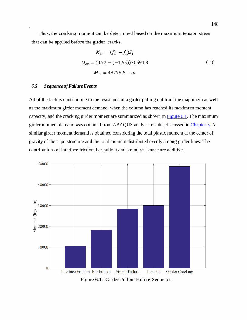
148 ``
Thus, the cracking moment can be determined based on the maximum tension stress
that can be applied before the girder cracks.
𝑀𝑀𝑐𝑐𝑏𝑏 = (𝑓𝑓𝑐𝑐𝑏𝑏 − 𝑓𝑓1)𝑆𝑆1
6.18 𝑀𝑀𝑐𝑐𝑏𝑏 = (0.72 − (−1.65))20594.8
𝑀𝑀𝑐𝑐𝑏𝑏 = 48775 𝑘𝑘 − 𝑠𝑠𝑠𝑠 6.5 Sequence of Failure Events
All of the factors contributing to the resistance of a girder pulling out from the diaphragm as well
as the maximum girder moment demand, when the column has reached its maximum moment
capacity, and the cracking girder moment are summarized as shown in Figure 6.1. The maximum
girder moment demand was obtained from ABAQUS analysis results, discussed in Chapter 5. A
similar girder moment demand is obtained considering the total plastic moment at the center of
gravity of the superstructure and the total moment distributed evenly among girder lines. The
contributions of interface friction, bar pullout and strand resistance are additive.
Figure 6.1: Girder Pullout Failure Sequence

149
The interface shear girder-diaphragm resistance will be overcome first. After that, the
girder will be relying on the extended bars and strands to resist it trying to pull out
of the diaphragm. The collective moment resistance of the extended strands and bars was
determined as 46,093 k-in, considering the impact of the portion of the top girder flange,
which is in compression and reduces the moment capacity.
This resistance is larger than the maximum girder bending moment of approximately
30,000 in-k, which is expected to occur when the column reaches its plastic moment
capacity. The largest girder moment was determined to occur when a partially cracked cap
beam and uncracked girders considered. The cap beam region, contained within the first
two girder lines was taken down to 5% of its uncracked stiffness, while the rest of the cap
beam was left uncracked. If the girders remain uncracked and the cap beam is completely
cracked (that is, the stiffness of the whole cap beam is down to 5% of its uncracked
stiffness), then the maximum girder moment demand was found to be approximately
36,500 k-in. This value is still significantly smaller than the resistance provided by the
extended bars and strands. This leads to the conclusion that fewer strands can be
extended, such that the total resistance to girder pull out would be equal to the maximum
girder moment demand. In that case, 4 extended strands, along with the extended
reinforcing bars would be sufficient to provide a 34,000 in-k moment resistance, ensuring
the girders will not pull out before the column has failed.
The bars extending from the girders into the diaphragm are currently considered to
serve as reinforcement for shear friction for transverse seismic loading, and to resist
pullout effects, arising in the girders due to creep. Thus, if the reinforcing bars, extended
from the girder into the diaphragm, are not considered to contribute to girder pullout
resistance during a seismic event, then 8 strands, with stresses fp = 260 ksi were
determined to provide resistance (of about 32,000 k-in), greater than the maximum girder
moment demand, obtained from either analysis or the assumption that all girders will
resist an equal portion of the seismic moment.

150 ``
The girder cracking moment is much greater than the largest girder bending moment
demand and thus the girders are not expected to crack by the time the column has reached
its plastic moment capacity.
The sequence of events influences the distribution of girder moment demand. It is
clear that the interface shear transfer fails first. If that is assumed to drop to zero
because the resistance is brittle, the subsequent behavior will depend on bar and strand
yielding. That implies essentially zero stiffness for incremental loading, in which case the
moment demand is uniform across all the girders and the same number of strands can be
extended from each girder.\
6.6 Design Guidelines
6.6.1. Design Procedure Based on all of the findings in this report, the following design procedure is recommended:
1. Determine the plastic moment of the column, Mp = 1.2Mn, and the corresponding
moment at the cg of the superstructure. This is the total moment to be distributed among
the girders. (See WSDOT BDM Section 5.1.3 Equation 5.1.3-2).
2. Determine the value of λLcb for the bent, and from it the ideal distribution of moment
among the girders, using Table 6.1. For values of parameters not addressed in the table,
the girder moments may be obtained using Equation 6.19.
𝑀𝑀𝑏𝑏,𝑏𝑏 = 𝑇𝑇𝑛𝑛𝑠𝑠𝑠𝑠𝑠𝑠ℎ �𝜆𝜆𝑃𝑃𝑐𝑐𝑏𝑏2𝑁𝑁𝐿𝐿
�
𝑠𝑠𝑠𝑠𝑠𝑠ℎ(𝜆𝜆𝑃𝑃𝑐𝑐𝑏𝑏) 𝑐𝑐𝐴𝐴𝑠𝑠ℎ � 𝜆𝜆𝑃𝑃𝑐𝑐𝑏𝑏 �1−𝑠𝑠 − 1/2𝑁𝑁𝐿𝐿
�� 6.19
where:
EI = flexural stiffness of one girder, including composite deck,
GJ = torsional stiffness of the cab beam cross-section,
i = girder line number,
Lcb = half of the cap beam length, for a single column bent; half of the column spacing for a
multi-column bent,

151
Lg = girder span length, if girders frame into the cap beam from only one side; 2/(1/L1 +
1/L2) if girders frame into the cap beam from both sides, where L1, L2 = individual girder
span lengths.
Mg,i = bending moment in girder i caused by longitudinal seismic loading,
NL = the number of girder lines along half of the cap beam,
To = maximum torque in the cap beam equal to half of the total seismic moment generated
by a single column and acting at the center of gravity of the superstructure,
λLcb = ratio of total stiffness of all girders to torsional stiffness of half the total length of the
cap beam. For girders in which the far end is free to rotate, λLcb = ( )cb
L
g LGJN
LEI
/23
. The
term 3EIg should be replaced by 4EIg when the far end of the girder is fixed against rotation.
2.1. For two-stage prismatic cap beams, the moment distribution is likely to be nearly
uniform.
2.2. For flush cap beams, it is likely that λLcb will be > 1.0 and the moment distribution
will not be uniform.
2.3. For tapered cap beams, Table 6.1 (or Equation 6.19) may be used if the torsional
stiffness is initially defined by the deepest section of the cap beam, and λLcb is then
increased by 20%. This will lead to a less uniform distribution of girder moments
than that found with a prismatic cap beam.
3. Adjust the girder moments from their ideal values to a practical distribution that can be
accommodated by an integral number of extended strands in each girder. The sum of the
adjusted moments shall be at least as large as the sum of the ideal moments, and the
adjustments should generally increase the moments in girders closer to the column. A
slight downwards adjustment in an individual girder moment is acceptable, especially in
a girder remote from the column.
4. Select strands and bars to develop the required moment resistance in each girder:
4.1. Use strands extended from the bottom flange, rather than reinforcing bars, to the
extent possible. (Reasoning: The strands are located with the greatest lever arm and
so are the most efficient way to resist moment. Strands are stronger than comparably
sized rebar, so fewer are needed. Strands may be fully anchored within the cap beam

152 ``
with strand vices, at the horizontal location that is most advantageous for satisfactory
joint performance. Strands are already well anchored in the girder, so no special
anchorage requirements are needed there. Strands are more flexible in bending than
rebar, so may more easily be moved in cases of conflict during construction.)
4.2. Extend each strand as far as possible through the cap beam (e.g. to a point 6 inches
inside the vertical diaphragm steel on the opposite face.) Anchor each strand with a
strand vice that is fully seated prior to girder shipment.
4.3. The pattern of strands extended from opposing girders at a common cap beam
should be chosen in such a way as to minimize the likelihood of conflicts.
4.4. To calculate the positive moment flexural resistance of the girder, assume that each
strand is stressed to its yield stress (e.g. 243 ksi). (Reasoning: by this means the
elongation of the strand will be < 1%, and the girder pullout from the cap beam will
be < 1.0”, when the column plastic capacity is reached. The strand will also pull the
girder back to its original position, with no residual displacement, after an event.)
4.5. If some of the rebar used in the present detail is retained, its contribution to the
flexural strength should be counted in order to minimize the number of extended
strands. (This is not recommended: the web rebar is located so that it is anchored
near the face of the cap beam, and may cause unnecessary joint shear stress or block
pullout damage during an extreme event.)

153
Table 6.1: Girder Moment Ratios as a Function of Stiffness Ratio λLcb
λLcb
NL = 2 NL = 3 NL = 4
𝑀𝑀𝑏𝑏,1
𝑇𝑇𝑛𝑛
𝑀𝑀𝑏𝑏,2
𝑇𝑇𝑛𝑛
𝑀𝑀𝑏𝑏,1
𝑇𝑇𝑛𝑛
𝑀𝑀𝑏𝑏,2
𝑇𝑇𝑛𝑛
𝑀𝑀𝑏𝑏,3
𝑇𝑇𝑛𝑛
𝑀𝑀𝑏𝑏,1
𝑇𝑇𝑛𝑛
𝑀𝑀𝑏𝑏,2
𝑇𝑇𝑛𝑛
𝑀𝑀𝑏𝑏,3
𝑇𝑇𝑛𝑛
𝑀𝑀𝑏𝑏,4
𝑇𝑇𝑛𝑛
0 0.250 0.250 0.167 0.167 0.167 0.125 0.125 0.125 0.125
0.2 0.251 0.249 0.168 0.166 0.166 0.126 0.125 0.125 0.124
0.4 0.255 0.245 0.172 0.166 0.163 0.129 0.126 0.123 0.122
0.6 0.261 0.239 0.177 0.164 0.158 0.135 0.126 0.121 0.118
0.8 0.269 0.231 0.185 0.163 0.152 0.142 0.127 0.118 0.113
1 0.278 0.222 0.195 0.161 0.144 0.150 0.128 0.114 0.107
1.2 0.289 0.211 0.206 0.158 0.136 0.160 0.129 0.110 0.101
1.4 0.301 0.199 0.218 0.155 0.127 0.171 0.130 0.105 0.094
1.6 0.313 0.187 0.230 0.152 0.118 0.182 0.131 0.100 0.086
1.8 0.326 0.174 0.243 0.148 0.108 0.194 0.131 0.095 0.079
2 0.338 0.162 0.257 0.144 0.099 0.206 0.132 0.090 0.072
2.2 0.350 0.150 0.270 0.140 0.090 0.219 0.131 0.085 0.065
2.4 0.362 0.138 0.283 0.136 0.081 0.231 0.131 0.080 0.058
2.6 0.373 0.127 0.295 0.132 0.073 0.243 0.130 0.075 0.052
2.8 0.384 0.116 0.307 0.127 0.066 0.255 0.129 0.070 0.046
3 0.394 0.106 0.319 0.122 0.059 0.266 0.128 0.065 0.041
3.2 0.403 0.097 0.330 0.118 0.052 0.277 0.126 0.061 0.036
3.4 0.412 0.088 0.341 0.113 0.047 0.287 0.124 0.056 0.032
3.6 0.420 0.080 0.351 0.108 0.041 0.297 0.122 0.052 0.028
3.8 0.427 0.073 0.360 0.104 0.037 0.307 0.120 0.049 0.025
4 0.434 0.066 0.369 0.099 0.032 0.316 0.117 0.045 0.022
Note: The numbers 1, 2, 3 and 4 refer to the girder lines. Line 1 is closest to the column.

154 ``
6.6.2. Design Example A reference structure with 6 girder lines and a single column bent was used in this design example, as it considers 3 girder lines along half of the cap beam.
Given:
Dc = 6.00’ column diameter,
f’c = 4.00 ksi specified concrete strength of deck concrete, Class 4000D,
db = 0.6” nominal strand diameter, area of strand = 0.217 in2,
fpu = 270 ksi specified tensile strength of prestressing strands,
fpy = 243 ksi for low relaxation strand,
ϕ = 1.00 resistance factor for extreme event limit state,
GTYP = WF74G; H = 74” girder depth,
A = 11¾” “A” dimension,
ts = 7” slab thickness,
Yt slab = 23.897” c.g. of superstructure to top of slab,
h = 125.103” distance from top of column to c.g. of superstructure,
L1 = 110’ Span length of span 1. Factor = 1.00 (two-span bridge),
L2 = 160’ Span length of span 2. Factor = 1.00,
Lcol = 25’ column clear height used to determine overstrength moments,
𝑀𝑀𝑝𝑝𝑛𝑛𝑒𝑒𝑛𝑛𝑝𝑝 = 16854 k-ft plastic overstrength moment at the top of the column,
𝑀𝑀𝑝𝑝𝑛𝑛𝐵𝐵𝑏𝑏𝑠𝑠𝑏𝑏 = 16963 k-ft plastic overstrength moment at the base of the column,
MSIDL = 520 k-ft moment due to SIDL per girder (based on BDM design example in Appendix 5-B10),
γp = 0.9
Design:
1. Total seismic moment at the center of gravity of the superstructure
𝑀𝑀𝑝𝑝𝑛𝑛𝐶𝐶𝐶𝐶 = 16854 + �
16854 + 1696325
� ∗125.103
12
𝑀𝑀𝑝𝑝𝑛𝑛𝐶𝐶𝐶𝐶 = 30956.03 𝑘𝑘 − 𝑓𝑓𝑡𝑡

155
2. Design moment per girder From Step 1, the maximum torque in the cap beam is equal to half of the total seismic
moment, or
𝑇𝑇𝑛𝑛 = 15478.015 𝑘𝑘 − 𝑓𝑓𝑡𝑡
Considering the following properties,
Eg = 5328 ksi,
Ecb = 3644 ksi,
Since ν = 0.2 for concrete and = 𝐸𝐸2(1+𝜈𝜈) ,
Gcb = 1518 ksi,
Ig = 1313000 in4 for a composite section including a WF74G girder with a 7” deck on top,
Lg = 12 * 2/(1/110 ft + 1/160 ft) = 1560”,
Lcb = 234”,
hcb = 149”,
bcb = 96” total (cross beam+ diaphragm),
Jcb = ℎ𝑐𝑐𝑐𝑐𝑏𝑏𝑐𝑐𝑐𝑐3
3�1 − 0.63𝑏𝑏𝑐𝑐𝑐𝑐
ℎ𝑐𝑐𝑐𝑐� = 26110000 in4, and
NL = 3,
Finally, considering pinned girder ends,
𝜆𝜆𝑃𝑃𝑐𝑐𝑏𝑏 = �3 �𝐸𝐸𝐼𝐼𝐿𝐿�𝑏𝑏
2𝑁𝑁𝐿𝐿(𝐶𝐶𝐺𝐺)𝑐𝑐𝑐𝑐
𝑃𝑃𝑐𝑐𝑏𝑏
The ratio 𝜆𝜆𝑃𝑃𝑐𝑐𝑏𝑏 was determined as 0.69 for the reference structure used here (ignoring the
lower crossbeam taper, and considering the cap beam section directly above the column,
which has the full height of 6’ for the cross beam and 6’-5” for the diaphragm).

156 ``
Using Table 1, the corresponding girder moment ratios, 𝑀𝑀𝑔𝑔,𝑖𝑖
𝑇𝑇𝑐𝑐 are as follows:
Girder no: 1 2 3 𝑀𝑀𝑏𝑏,𝑏𝑏
𝑇𝑇𝑛𝑛 0.181 0.164 0.156
The corresponding seismic moment per girder is
The span moment distribution factors K1 and K2 are
Equation 6.19 and Table 6.1 are based on the assumption that the two girders in each line
each resist 50% of the girder line moment. If the two girder spans differ, the moments
should be modified in accordance with the span lengths, using the factors K1 and K2 in place
of 0.50. The final girder moment demands can be determined as
𝐾𝐾0.5𝑀𝑀𝑏𝑏,𝑏𝑏 − 0.9𝑀𝑀𝑆𝑆𝐼𝐼𝑆𝑆𝐿𝐿.
Thus, the design moment for each girder is as follows:
3. Number of extended strands 3.1. Excluding the contribution of extended girder web and bottom flange reinforcing bars
into the diaphragm
The c.g. of extended strands to the bottom of the girder was taken as 3”, so the lever arm, d,
is 82.25”.
Girder no: 1 2 3 𝑀𝑀𝑏𝑏,𝑏𝑏 (k-ft) 2797 2535 2407
K1 =𝑃𝑃2
𝑃𝑃1 + 𝑃𝑃2=
160110 + 160
= 0.593 and
K2 =𝑃𝑃1
𝑃𝑃1 + 𝑃𝑃2=
110110 + 160
= 0.407
Girder 1 2 3 𝑀𝑀𝑏𝑏,𝐿𝐿1 (k-ft) 2847 2536 2385 𝑀𝑀𝑏𝑏,𝐿𝐿2 (k-ft) 1811 1597 1493
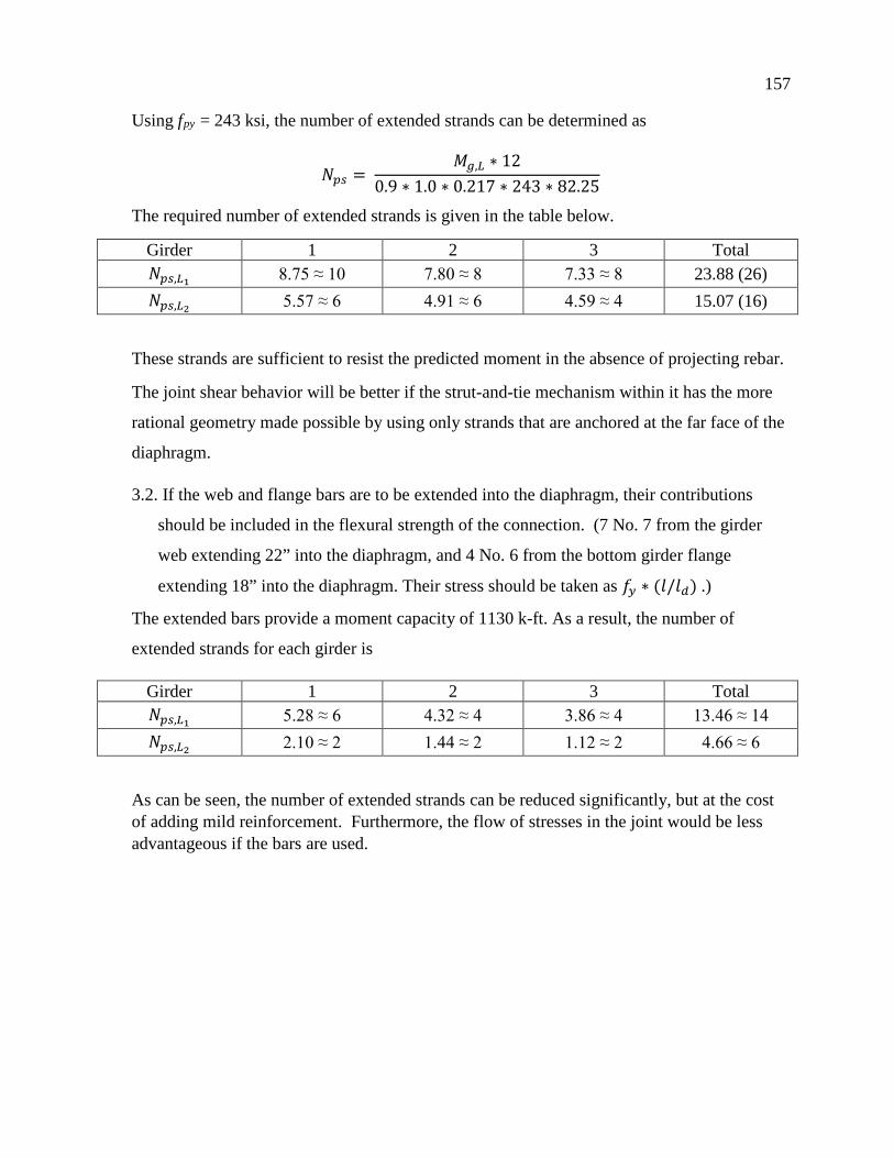
157
Using fpy = 243 ksi, the number of extended strands can be determined as
𝑁𝑁𝑝𝑝𝑠𝑠 = 𝑀𝑀𝑏𝑏,𝐿𝐿 ∗ 12
0.9 ∗ 1.0 ∗ 0.217 ∗ 243 ∗ 82.25
The required number of extended strands is given in the table below.
These strands are sufficient to resist the predicted moment in the absence of projecting rebar.
The joint shear behavior will be better if the strut-and-tie mechanism within it has the more
rational geometry made possible by using only strands that are anchored at the far face of the
diaphragm.
3.2. If the web and flange bars are to be extended into the diaphragm, their contributions
should be included in the flexural strength of the connection. (7 No. 7 from the girder
web extending 22” into the diaphragm, and 4 No. 6 from the bottom girder flange
extending 18” into the diaphragm. Their stress should be taken as 𝑓𝑓𝑦𝑦 ∗ (𝑙𝑙/𝑙𝑙𝑒𝑒) .)
The extended bars provide a moment capacity of 1130 k-ft. As a result, the number of
extended strands for each girder is
As can be seen, the number of extended strands can be reduced significantly, but at the cost of adding mild reinforcement. Furthermore, the flow of stresses in the joint would be less advantageous if the bars are used.
Girder 1 2 3 Total 𝑁𝑁𝑝𝑝𝑠𝑠,𝐿𝐿1 8.75 ≈ 10 7.80 ≈ 8 7.33 ≈ 8 23.88 (26) 𝑁𝑁𝑝𝑝𝑠𝑠,𝐿𝐿2 5.57 ≈ 6 4.91 ≈ 6 4.59 ≈ 4 15.07 (16)
Girder 1 2 3 Total 𝑁𝑁𝑝𝑝𝑠𝑠,𝐿𝐿1 5.28 ≈ 6 4.32 ≈ 4 3.86 ≈ 4 13.46 ≈ 14 𝑁𝑁𝑝𝑝𝑠𝑠,𝐿𝐿2 2.10 ≈ 2 1.44 ≈ 2 1.12 ≈ 2 4.66 ≈ 6

158 ``
Chapter 7
SUMMARY AND CONCLUSIONS
7.1 Summary
Precast prestressed bridges in Washington State are designed to resist longitudinal
seismic forces by frame action. Moments must therefore be transferred from the ends of
the girders, where they are manifested as bending, into the cap beam, where they are
manifested as torsion. Consequently, positive moment connections are needed at the
girder ends, and they are presently achieved by extending some of the strands located in
the bottom flange of the girder into the cast-in-place diaphragm, where they are anchored
with strand vices and bearing plates. That hardware configuration can cause conflicts and
difficulties during construction. The goals of this research were to investigate the existing
method of making the positive moment connection and, if possible, to develop a new one
that would be easier to construct. The goals were addressed using a combination of
laboratory testing and structural analysis. The first two tasks, associated with the
anchorage capacity of strands equipped with barrel anchors, were completed using
laboratory tests. The last task, in which the moment demand at each girder end was
evaluated, was conducted using structural analysis.
The performance of a single anchorage device, and in particular the possibility of local
concrete crushing behind the strand anchor, was first investigated by physical testing. It
was found that a barrel anchor, with no backing plate, was easily sufficient to resist the
force imposed by a strand at incipient fracture.
Second, the possibility of a group of strands breaking out from the diaphragm was
evaluated. Tests were carried out on strands, anchored by strand vices, grouped in various
patterns and embedded to various depths in concrete blocks representing a diaphragm. It
was found that the results were closely predicted by the Concrete Capacity Design
method, which can therefore be used to predict the minimum embedment length required
to ensure that strand fracture takes place prior to a group breakout failure mode.

159
Third, the distribution of girder end moments across the bridge was evaluated using Finite
Element Analysis. The important parameters were the flexural properties of the girders and the
torsional properties of the cap beam. The outcome focused on the girder end moments when the
column reached its full flexural capacity.
7.2 Conclusions
• Resistance of a single anchor. A barrel anchor, with no backing plate, is easily
sufficient to resist, without damage to the anchor or bearing failure of the concrete,
the force exerted by a strand at incipient fracture. The high resistance to bearing
stresses (measured at approximately 100 ksi on concrete with f’c ≈ 4 ksi) is
attributed to very efficient confinement behind the anchor.
• Resistance of a group of strands to failure by breakout. The Concrete Capacity
Design method predicted very accurately the failure loads measured in the tests
conducted for this project. Those tests, with the tests originally used to develop
the method, provide verification of the method, which can therefore be used to
evaluate the minimum embedment depth needed to ensure that ductile strand
yield and fracture precede brittle group breakout failure.
• Distribution of girder moment demand across the bridge. For bridges
constructed with a two-stage cap-beam, such as is used extensively in
Washington State, the cap beam system is sufficiently stiff in torsion compared
to the flexural stiffness of the girders that the moment demand in the end of each
girder is almost uniform across the width of the bridge. The end moment used
for design, and consequently the number of strands that need to be extended
from each girder, may thus be reduced below the values required by the existing
design method. That method was developed from tests conducted on a system in
which the ratio of cap beam torsional stiffness to girder bending stiffness was
much lower than that typical of Washington State bridges.

160 ``
7.3 Recommendations
7.3.1 Recommendations for Implementation
• Extended strands, up to and including 0.6” diameter, should be equipped with a
barrel anchor alone. No backing plate is necessary.
• Strands should be extended as far as possible across the cap beam to achieve
the best transfer of moment into the cap beam. Terminating the strand just
inside the vertical reinforcement at the far side of the cap beam maximizes the
structural benefits and minimizes the construction difficulties.
• Girder end moments may be determined using the approach outlined in Section
6.6 of this report. In most cases, that will lead to equal moments in each girder
and the smallest possible number of strands extending from each girder.
• Consideration should be given to eliminating the non-prestressed bar
reinforcement in the girder ends, and generating the force required for vertical
shear friction in the web from the extended strands alone. This would simplify
fabrication of the girders and reduce the possibility of bar conflicts on site.
7.3.2 Recommendations for Further Research
• The research conducted here addressed only right bridges. The anchorage capacities
are expected to remain unchanged in skew bridges, so the primary need is to
determine the moment demands in skew bridges. Preliminary hand calculations
suggest that, in a skew bridge, the cap beam behaves as if it were stiffer than in a
comparable right bridge, in which case the girder end moments would be distributed
even more uniformly than was found here. However, that tentative finding should be
investigated using FEA.

161
REFERENCES AASHTO (2009). AASHTO Guide Specifications for LRFD Seismic Bridge Design. American
Association of State Highway and Transportation Officials, American Association of
State Highway and Transportation Officials, 444 North Capitol Street, NW Suite 249,
Washington, DC 20001, United States, 1st Edition.
AASHTO (2012). AASHTO LRFD Bridge Design Specifications. American Association of
State Highway and Transportation Officials, American Association of State Highway
and Transportation Officials, 444 North Capitol Street, NW Suite 249, Washington, DC
20001, United States, 6th Edition.
ACI318 (2011). Building Code Requirements for Structural Concrete (ACI 318-11) and Com-
mentary. American Concrete Institute, American Concrete Institute, 38800 Country Club
Drive, Farmington Hills, MI 48331, United States.
ASTM (2015). Standard Test Method for Tension Testing of Metallic Materials. U.S. De-
partment of Defense, ASTM International, 100 Barr Harbor Drive, West Conshohocken,
PA 19428-2959, United States, 15a Edition.
Balmer, G. G. (1949). “Shearing Strength of Concrete Under High Triaxial Stress -
Compu- tation of Mohr’s Envelope as a Curve.” Structural Research Laboratory Report No.
SP-23,
U.S. Dept. of the Interior, Bureau of Reclamation, Denver, Colorado, 1–26.
Chuan-Zhi, W., Zhen-Hai, G., Zhen-Hai, G., and Xiu-Qin, Z. (1987). “Experimental
Inves- tigation of Biaxial and Triaxial Compressive Concrete Strength.” ACI Material
Journal, 84(2), 92–100.
162 ``
Fuchs, W., Eligehausen, R., and Breen, J. E. (1995). “Concrete Capacity Design (CCD)
Approach for Fastening to Concrete.” ACI Strucutral Journal, 92(1), 73–94.
Hawkins, N. M. (1968). “The Bearing Strength of Concrete Loaded Through Rigid Plates.”
Magazine of Concrete Research, 20(62), 31–40. Hibbeler, R. C. (2011). Mechanics of Materials, Custom Edition for the University of
Wash- ington. Pearson Prentice Hall.
Holombo, G. J. (1999). “Seismic Design of Precast Girder Bridges.” PhD Dissertation,
University Of California, San Diego, San Diego, California, United States.
Holombo, J., Priestley, M. J. N., and Seible, F. (2000). “Continuity of Precast Prestressed
Spliced-Girder Bridges under Seismic Loads.” PCI Journal, 45(2), 40–63.
Marsh, M. L., Stringer, S. J., Stanton, J. F., Eberhard, M. O., Haraldsson, O. S., Tran,
H. V., Khaleghi, B., Schultz, E., and Seigurant, S. (2013). “Precast Bent System for
High Seismic Regions.” Report no., Federal Highway Administration, United States.
Miller, R. A., Castrodale, R., Mirmiran, A., and Hastak, M. (2004). “Connection of
simple- span precast concrete girders for continuity.” Report no., National Cooperative
Highway Research Program, Transportation Research Board, Business Office 500 Fifth
Street NW, Washington DC 20001, United States.
Newhouse, C. D., Roberts-Wollmann, C. L., Cousins, T. E., and Davis, R. T. (2007).
“Com- parison of Strands and Bars for Positive Moment Connection of Continuous
Precast Con- crete Bulb-Tee Girders.” PCI Journal, 52(3), 18–28.
Newman, K. and Newman, J. (1971). “Failure Theories and Design Criteria for Plain Con-
crete.” Proceedings for International Civil Engineering Material Conference on Structural,
Solid Mechanics and Engineering Design, London, Wiley-Interscience, New York, NY,
963–995.

163
Noppakunwijai, P., Jongpitakseel, N., Ma, Z. J., Yehi, S. A., and Tadros, M. K. (2002).
“Pullout Capacity of Non-Prestressed Bent Strands for Prestressed Concrete Girders.”
PCI Journal, 47(4), 90–103.
Owen, L. M. (1998). “Stress-Strain Behaviour of Concrete Confined by Carbon Fiber
Jack- eting.” M.S. thesis, University of Washington, United States.
PCI (2004). PCI Design Handbook Precast and Prestressed Concrete. Precast/Prestressed
Concrete Institute, Precast/Prestressed Concrete Institute, 209 W Jackson Blvd, Suite
500, Chicago, Illinois 60606, United States, 6th Edition.
Pilkey, W. D. (2005). Formulas for Stress, Strain, and Structural Matrices, Second Edition.
John Wiley & Sons, Inc. Priestley, M. J. N., Seible, F., and Calvi, G. M. (1996). Seismic Design and Retrofit of Bridges.
John Wiley & Sons, Inc.
Richart, F. E., Brandtzaeg, A., and Brown, R. L. (1929). “The Failure of Plain and Spirally
Reinforced Concrete in Compression.” University of Illinois Bulletin, Vol. 26, Engineering
Experiment Station, University of Illinois at Urbana-Champaign, 1–74.
Stanton, J. F. (2002). Torsion, Lecture Notes, CEE220 Mechanics of Materials, University
of Washington, delivered in 2002.
Wight, J. K. and MacGregor, J. G. (2012). Reinforced Concrete: Mechanics and Design.
Pearson Education Inc. WSDOT (2015). WSDOT Bridge Design Manual (LRFD). Washington State Department of
Transportation, Washington State Department of Transportation, Bridge and Structures
Office, PO Box 47340, Olympia, WA 98504, United States, M 23-50.14 Edition.

164 ``

Americans with Disabilities Act (ADA) Information: This material can be made available in an alternate format by emailing the Office of Equal Opportunity at [email protected] or by calling toll free, 855-362-4ADA(4232). Persons who are deaf or hard of hearing may make a request by calling the Washington State Relay at 711.
Title VI Statement to Public: It is the Washington State Department of Transportation’s (WSDOT) policy to assure that no person shall, on the grounds of race, color, national origin or sex, as provided by Title VI of the Civil Rights Act of 1964, be excluded from participation in, be denied the benefits of, or be otherwise discriminated against under any of its federally funded programs and activities. Any person who believes his/her Title VI protection has been violated, may file a complaint with WSDOT’s Office of Equal Opportunity (OEO). For additional information regarding Title VI complaint procedures and/or information regarding our non-discrimination obligations, please contact OEO’s Title VI Coordinator at (360) 705-7082.