1

Cost-Sensitive Classifier Selection Using the ROC Convex Hull Method

Ross Bettinger SAS Institute, Inc.

180 N. Stetson Ave. Chicago, IL 60601

Ross.Bettinger@SAS.com

Abstract One binary classifier may be preferred to another based on the fact that it has better prediction accuracy than its competitor. Without additional information describing the cost of a misclassifi-cation, accuracy alone as a selection criterion may not be a sufficiently robust measure when the distribution of classes is greatly skewed or the costs of different types of errors may be signifi-cantly different. The receiver operating characteristic (ROC) curve is often used to summarize binary classifier performance due to its ease of interpretation, but does not include misclassification cost informa-tion in its formulation. Provost and Fawcett [5, 7] have developed the ROC Convex Hull (ROCCH) method that incorporates techniques from ROC curve analysis, decision analysis, and computational geometry in the search for the optimal classifier that is robust with respect to skewed or imprecise class distributions and disparate misclassification costs. We apply the ROCCH method to several datasets using a variety of modeling tools to build bi-nary classifiers and compare their performances using misclassification costs. We support Pro-vost, Fawcett, and Kohavi’s claim [6] that classifier accuracy, as represented by the area under the ROC curve, is not an optimal criterion in itself for choosing a classifier, and that by using the ROCCH method, a more appropriate classifier may be found that realistically reflects class dis-tribution and misclassification costs.

1. Introduction A typical goal in extracting knowledge from data is the production of a classification rule that will assign a class membership to a future event with a specified probability. The classification rule may take the following form: “If the probability of response is greater than 0.14159 then send the targeted individual an invitation to buy our product or service. Otherwise, do not so-licit.” This is an example of a binary classification rule that assigns a probability to a class or set of mutually exclusive events. In this case, the classes are {“Solicit”, “Do not solicit”}. There are a number of algorithms that produce classification rules, each with its strengths and weaknesses, parameter settings and data requirements. We are concerned here not with the algo-rithms themselves but the circumstances surrounding the production of classification rules. As others have indicated, the most accurate classifier is not necessarily the optimal classifier for all situations (Adams and Hand [1], Provost and Fawcett [5, 7]). Classifiers that do not properly ac-count for greatly skewed class distributions of a binary response variable or that assume equal misclassification costs when such is not the case may return decisions that are inaccurate and very costly. For example, in fraud detection, actual cases of fraud are usually quite rare and often

2

reflect similar patterns of behavior as legitimate activities. However, the cost of missing a fraudulent act may be quite high to a merchant in comparison to wrongly questioning someone’s legitimate use of, say, a credit card to make a nominal purchase and thereby incurring a card-member’s displeasure. Hence, algorithms that produce realistic classification rules must include the plenitude or paucity of the events being modeled, and must also utilize misclassification costs in the rule production process.

2. Cost Considerations for Binary Classifiers1 We observe that a binary classifier assigns an object, which will usually be an observation, a case, or, in practical terms, a data vector, to one of two classes, and that the decision regarding the class assignment will be either correct or incorrect. Usually, the assignment to a class is de-scribed in terms of a future event, e.g., “Solicit/Do not solicit”, or “Yes/No” or some other bi-nary-valued decision expressed in terms of a business problem. From the standpoint of predicted class membership or outcome {Event, Nonevent} versus actual class membership {event, non-event}, we have a 2x2 classification table describing the four possible {predicted outcome, actual outcome} states. Table 1 enumerates these outcomes. Table 1. Classification table of class membership Predicted Event, E Predicted Nonevent, N Actual Event, e (E, e) True Positive (TP) (N, e) False Negative (FN) Actual Nonevent, n (E, n) False Positive (FP) (N, n) True Negative (TN) The true positive rate is also called “sensitivity,” and the true negative rate is also called “speci-ficity,” in the machine learning literature. A critical concept in the discussion of decisions is the definition of an event. We may say that an observation or instance, I, has been classified into class e with probability p(e|I) if the classifier assigns a probability cutoffpIp ≥)( where cutoffp may have been previously defined according to

some business rule or operational consideration. We may, without loss of generality, omit any processing costs of a decision since such costs will be incurred regardless of the decision issued by the classifier (Adams and Hand [1]). We assume that the only cost of a correct decision is the processing cost, so that c(E, e) = c(N, n) = 0. We may assume the existence of an exact cost function, c(predicted class, actual class), that will as-sess a cost for misclassification of an event to a wrong class. Assuming that predicted decisions are {E, N} and that the respective actual event and nonevent class memberships are {e, n}, we can represent the costs of misclassifying an event in terms of false positive error as c(E, n) and false negative error as c(N, e). The distribution of class memberships are represented by the prior probabilities p(e) and p(n) = 1 – p(e). In terms of prior class membership, the correctly-predicted (true positive) event classification rate (TP) is

1 We follow the discussion of Provost and Fawcett [7] in this section and the sequel.

3

TP = p(E|p) = }{#

}{#

eventstotal

eventspredicted,

the correctly-predicted (true negative) nonevent classification rate (TN) is

TN = p(N|n) = }{#

}{#

noneventstotal

noeventspredicted,

the falsely-predicted (false positive) event classification rate (FP) is

FP = p(E|n) = }{#

}{#

noneventstotal

eventspredicted,

and the falsely-predicted (false negative) nonevent classification rate (FN) is

FN = p(N|e) = }{#

}{#

eventstotal

noneventspredicted,

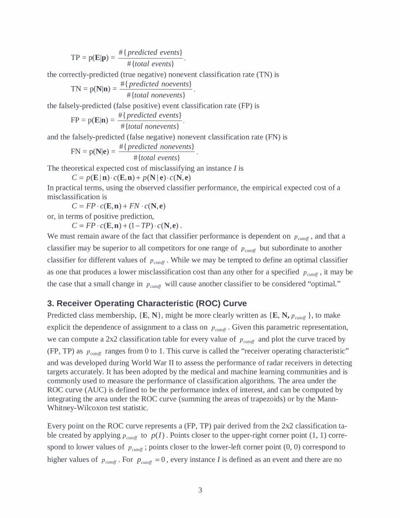
The theoretical expected cost of misclassifying an instance I is ),()|(),()|( eNeNnEnE cpcpC ⋅+⋅=

In practical terms, using the observed classifier performance, the empirical expected cost of a misclassification is

),(),( eNnE cFNcFPC ⋅+⋅= or, in terms of positive prediction,

),()1(),( eNnE cTPcFPC ⋅−+⋅= . We must remain aware of the fact that classifier performance is dependent on cutoffp , and that a

classifier may be superior to all competitors for one range of cutoffp but subordinate to another

classifier for different values of cutoffp . While we may be tempted to define an optimal classifier

as one that produces a lower misclassification cost than any other for a specified cutoffp , it may be

the case that a small change in cutoffp will cause another classifier to be considered “optimal.”

3. Receiver Operating Characteristic (ROC) Curve Predicted class membership, {E, N}, might be more clearly written as {E, N, cutoffp }, to make

explicit the dependence of assignment to a class on cutoffp . Given this parametric representation,

we can compute a 2x2 classification table for every value of cutoffp and plot the curve traced by

(FP, TP) as cutoffp ranges from 0 to 1. This curve is called the “receiver operating characteristic”

and was developed during World War II to assess the performance of radar receivers in detecting targets accurately. It has been adopted by the medical and machine learning communities and is commonly used to measure the performance of classification algorithms. The area under the ROC curve (AUC) is defined to be the performance index of interest, and can be computed by integrating the area under the ROC curve (summing the areas of trapezoids) or by the Mann-Whitney-Wilcoxon test statistic. Every point on the ROC curve represents a (FP, TP) pair derived from the 2x2 classification ta-ble created by applying cutoffp to )(Ip . Points closer to the upper-right corner point (1, 1) corre-

spond to lower values of cutoffp ; points closer to the lower-left corner point (0, 0) correspond to

higher values of cutoffp . For 0=cutoffp , every instance I is defined as an event and there are no

4

false positives. This point on the ROC curve is located at (1, 1). For 1=cutoffp , every instance I is

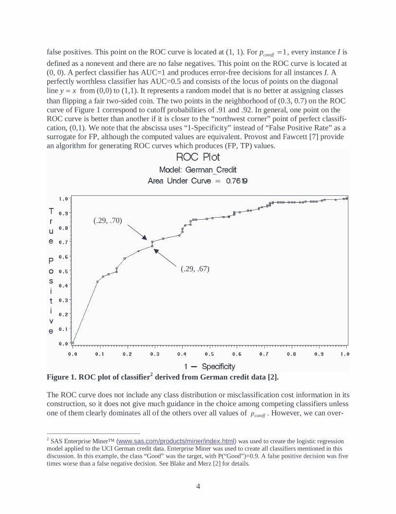
defined as a nonevent and there are no false negatives. This point on the ROC curve is located at (0, 0). A perfect classifier has AUC=1 and produces error-free decisions for all instances I. A perfectly worthless classifier has AUC=0.5 and consists of the locus of points on the diagonal line xy = from (0,0) to (1,1). It represents a random model that is no better at assigning classes than flipping a fair two-sided coin. The two points in the neighborhood of (0.3, 0.7) on the ROC curve of Figure 1 correspond to cutoff probabilities of .91 and .92. In general, one point on the ROC curve is better than another if it is closer to the “northwest corner” point of perfect classifi-cation, (0,1). We note that the abscissa uses “1-Specificity” instead of “False Positive Rate” as a surrogate for FP, although the computed values are equivalent. Provost and Fawcett [7] provide an algorithm for generating ROC curves which produces (FP, TP) values.

Figure 1. ROC plot of classifier2 derived from German credit data [2]. The ROC curve does not include any class distribution or misclassification cost information in its construction, so it does not give much guidance in the choice among competing classifiers unless one of them clearly dominates all of the others over all values of cutoffp . However, we can over-

2 SAS Enterprise Miner™ (www.sas.com/products/miner/index.html) was used to create the logistic regression model applied to the UCI German credit data. Enterprise Miner was used to create all classifiers mentioned in this discussion. In this example, the class “Good” was the target, with P(“Good”)=0.9. A false positive decision was five times worse than a false negative decision. See Blake and Merz [2] for details.

(.29, .67)

(.29, .70)

5

lay class distribution and misclassification cost on the ROC curve. Per Metz, et al. [3], the aver-age cost per decision computed by a classifier can be represented by the equation

)()|(),(

),()(

0

0

jji j

iji

i jjiij

ActualPlActuaPredictedPActualedictedPrcC

ActualPredictedPCosticationMisclassifCC

∑∑

∑∑

⋅+=

⋅+=

in which 0C is the fixed “overhead” or processing cost of a decision, iPredicted ={E, N}, and

jActual ={e, n}. Then for the 2x2 classification table, the equation becomes

)()|(),()()|(),(

)()|(),()()|(),(0

nnNnNnnEnE

eeNeNeeEeE

PPcPPc

PPcPPcCC

⋅⋅+⋅⋅+⋅⋅+⋅⋅+=

We are implicitly assuming that overhead costs and misclassification costs may be combined ad-ditively. Differentiating )|( eEP by )|( nEP and equating the resulting expression to 0 to find the point at which average cost is minimized, we have

),(),(

),(),(

)(

)(

)|(

)|(

eEeNnNnE

en

nEeE

cc

cc

P

P

dP

dP

−−= ,

which becomes

),(

),(

)(

)(

)|(

)|(

eNnE

en

nEeE

c

c

P

P

dP

dP =

since we have assumed that the cost of a correct decision is the processing cost, which may be disregarded. We observe that, for a skewed distribution where P(e) is relatively rare, say, P(e) < .05, and/or for c(E, n)/c(N, e) >> 1, the slope of the curve will be high, indicating that a high value of cutoffp will be required for efficient minimum-cost decision-making. Contrapositively,

where P(e) is not rare and the misclassification costs are roughly equal, cutoffp will be lower and

will indicate less-precise decision-making due to a higher tolerance for false positive decisions. We may represent the slope of this line by choosing adjacent points )TP,FP( 11 and )TP,FP( 22 to form the isoperformance line (Provost and Fawcett, [5, 7])

),(

),(

)(

)(

12

12

eNnE

en

c

c

P

P

FPFP

TPTP =−−

(1)

for which the same cost applies to all classifiers tangent to the line. Hence, by computing slopes between adjacent pairs of ROC curve points, we may find the exact point (or interval) at which the isoperformance line is tangent to the ROC curve and thus determine cutoffp .

4. ROC Convex Hull (ROCCH) Method More than one ROC curve may be plotted on the same (FP, TP) axes. In this case, visual inspec-tion of the curves may not suffice to identify an optimal classifier. For example, Figure 2 shows three ROC curves overlaid on the same graph, each created by a different algorithm applied to the same set of data. Ensemble classifiers were created from the German credit data using four-fold cross-validation. The logistic regression model appears to be superior to either the neural network or the decision tree model over most, but not all, of the decision space. The choice of classifier is not obvious unless there is prior information with which to determine cutoffp . As dis-

cussed above, it is dependent on the class distribution and misclassification costs, which are not included in the visual display.

6

Figure 2. ROC plots of classifiers derived from German credit data [2]. Provost and Fawcett [5, 7] have described in detail the creation of the ROC convex hull, in which the envelope of “most-northwest” (i.e., closest to the optimal (0,1) point) points of several overlaid ROC curves is plotted3. They prove that the isoperformance line is tangent to a point (or interval) on the convex hull, and that the convex hull represents the locus of optimal classifier points under the class distribution assumptions corresponding to the slope of the isoperformance line. Figure 3 shows the convex hull of the classifiers plotted in ROC space for the German credit data.

3 Provost and Fawcett used an implementation of Graham’s scan to compute the set of points on the convex hull. The PERL implementation of the ROCCH algorithm and additional publications on this topic are available at http://www.hpl.hp.com/personal/Tom_Fawcett/ROCCH/index.html.

7

Figure 3. ROC curves and convex hull of classifiers derived from German credit data [2]. We see that the convex hull is composed of the “most-northwest” segments of the dominant clas-sifier between a pair of points in ROC space. Figure 4 includes the isoperformance line, which indicates the minimum-cost classifier (with re-spect to class distribution and misclassification costs) at the point of tangency. In this example, the logistic regression model did the best job of classifying credit applicants into “Good” and “Bad” classes.

8

Figure 4. ROC curves and convex hull with isoperformance line.

5. Applying the ROCCH Method to Select Classifiers The isoperformance line, which is tangent to the ROCCH at the point (or interval, in the case of tangency to a line segment on the convex hull) of minimum expected cost, indicates which clas-sifier to use for a specified combination of class distribution and misclassification costs. Ensem-ble classifiers were created from the German credit data using four-fold cross-validation. Cross-validation is necessary to smooth out the variation within a set of ROC curves and present a more realistic portrayal of classifier performance than might result from a single model. The isoperformance line in Figure 4 at the point (0.3467, 0.8229) is tangent to the ROC curve of the logistic regression classifier and indicates that this classifier is optimal for the specified class distribution and misclassification costs specified. Furthermore, the ROCCH method indicates the range of slopes over which a particular classifier is optimal with respect to class and costs. Table 2 describes all classifier points on the convex hull, and the classifier associated with each point. Table 2. All classifier points on ROCCH and associated German credit ensemble classifier Point (FP, TP) Classifier [0.0000, 0.0000] All Negative [0.0400, 0.2571] Logistic Regression [0.0800, 0.3714] Logistic Regression [0.1200, 0.4686] Logistic Regression

9

[0.3200, 0.7886] Logistic Regression [0.3467, 0.8229] Logistic Regression [0.5200, 0.8914] Logistic Regression [0.7067, 0.9543] Neural Network [1.0000, 1.0000] All Positive Table 3 contains the range of slopes at each point of isoperformance line tangency, as well as the classifier that is optimal over each range of slopes. Table 3. Range of slopes, point of isoperformance line tangency, and associated German credit ensemble classifier Slope Range Right Boundary Classifier [0.0000, 0.1558] [1.0000, 1.0000] All Positive [0.1558, 0.3367] [0.7067, 0.9543] Neural Network [0.3367, 0.3956] [0.5200, 0.8914] Logistic Regression [0.3956, 1.2857] [0.3467, 0.8229] Logistic Regression [1.2587, 1.6000] [0.3200, 0.7886] Logistic Regression [1.6000, 2.4286] [0.1200, 0.4686] Logistic Regression [2.4286, 2.8571] [0.0800, 0.3714] Logistic Regression [2.8571, 6.4286] [0.0400, 0.2571] Logistic Regression [6.4286, ∞] [0.0000, 0.0000] All Negative We can use the information in Table 3 to perform sensitivity analysis by computing the misclas-

sification cost ratio, ),(

),(

eNnE

c

c from Equation 1. Given the left and right ranges of the slope over

which a particular classifier is optimal, we can compute the ratio of false positive cost to false negative cost as a measure of classifier sensitivity to change in misclassification costs. Using the German credit ensemble classifiers as an example, with priors P(Event=“Good”) = 0.9 and P(Nonevent=“Bad”)=0.1, we can collapse Table 3 into two entries, as shown in Table 4. Table 4. Range of slopes, misclassification cost ratio range, and associated German credit ensemble classifier Slope Range FP/FN Cost Ratio Range Classifier [0.1558, 0.3367] [1.4022/1, 3.0303/1] Neural Network [0.3367, ∞] [3.0303/1, ∞] Logistic Regression Clearly, the logistic regression ensemble classifier is less misclassification cost-sensitive and hence more robust than the neural network ensemble classifier, and the decision tree ensemble classifier is not even competitive in this example for this particular class distribution. Similarly, for a specified range of misclassification costs, the range of slopes may be computed as a meas-ure of sensitivity to changes in class distribution. It may be of interest to note that the ROCCH has the greatest area under the ROC curve (AUC) (Provost and Fawcett [5]). For this set of data, the logistic regression ensemble classifier is optimal (given class distribution and misclassifica-tion costs) and also has the largest AUC (ranked second after the ROCCH classifier). Table 5 lists the AUC for the ROCCH and each ensemble classifier.

10

Table 5. Classifier and area under ROC curve for German Credit ensemble classifiers Classifier Area Under ROC Curve ROC Convex Hull 0.7892 Logistic Regression 0.7764 Neural Network 0.7422 Decision Tree 0.7139 Another model was built using data from a direct marketing application4. For this model, the av-erage revenue in response to a solicitation was $90, and the cost of mailing a catalog was $10. The response rate was 12%. Models were built using tenfold cross validation, and the results are presented in Figure 5 and Table 6. For this model, the profit-maximizing neural network model was not the most accurate classifier, which was logistic regression. In accordance with Provost, Fawcett, and Kohavi’s [6] claim, local performance determined by class distribution and mis-classification costs is better than optimal performance as measured by AUC.

Figure 5. ROC curves and convex hull with isoperformance line for Catalog Direct Mail model

4 This dataset, CUSTDET1, comes with the SAS Enterprise Miner sample library. It is available from the author upon request.

11

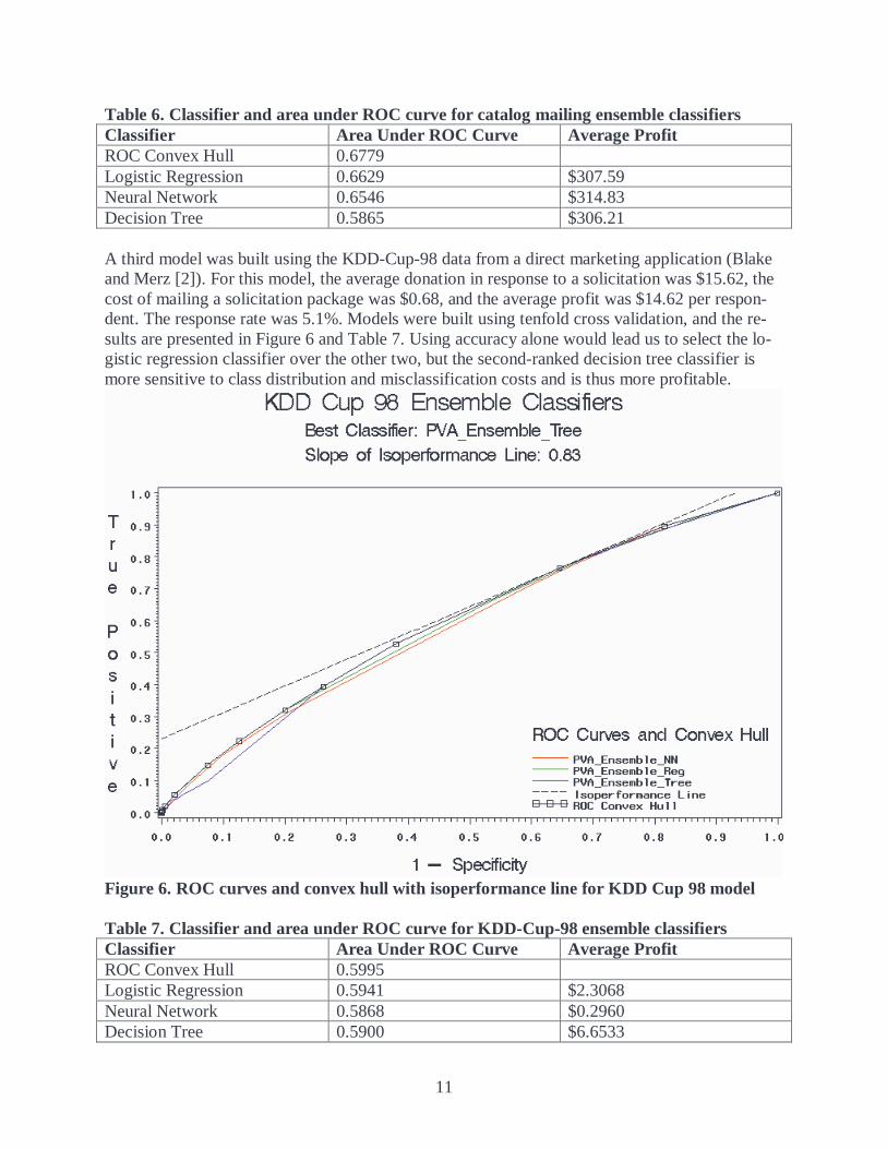
Table 6. Classifier and area under ROC curve for catalog mailing ensemble classifiers Classifier Area Under ROC Curve Average Profit ROC Convex Hull 0.6779 Logistic Regression 0.6629 $307.59 Neural Network 0.6546 $314.83 Decision Tree 0.5865 $306.21 A third model was built using the KDD-Cup-98 data from a direct marketing application (Blake and Merz [2]). For this model, the average donation in response to a solicitation was $15.62, the cost of mailing a solicitation package was $0.68, and the average profit was $14.62 per respon-dent. The response rate was 5.1%. Models were built using tenfold cross validation, and the re-sults are presented in Figure 6 and Table 7. Using accuracy alone would lead us to select the lo-gistic regression classifier over the other two, but the second-ranked decision tree classifier is more sensitive to class distribution and misclassification costs and is thus more profitable.

Figure 6. ROC curves and convex hull with isoperformance line for KDD Cup 98 model Table 7. Classifier and area under ROC curve for KDD-Cup-98 ensemble classifiers Classifier Area Under ROC Curve Average Profit ROC Convex Hull 0.5995 Logistic Regression 0.5941 $2.3068 Neural Network 0.5868 $0.2960 Decision Tree 0.5900 $6.6533

12

6. Summary The ROCCH methodology for selecting binary classifiers explicitly includes class distribution and misclassification costs in its formulation. It is a robust alternative to whole-curve metrics like AUC, which reports global classifier performance but which may not indicate the best clas-sifier (in the least-cost sense) for the range of operating conditions under which the classifier will assign class memberships.

Acknowledgements We thank Drs. Provost and Fawcett, who generously answered questions and provided useful advice.

References 1. Adams, N.M., and D. J. Hand (1999). Comparing Classifiers When the Misallocation Costs

are Uncertain. Pattern Recognition, Vol. 32, No. 7, pp. 1139-1147.

��� Blake, C.L. and C. J. Merz (1998). UCI Repository of machine learning databases. Irvine, CA: University of California, Department of Information and Computer Sci-ence. Available from World Wide Web: <http://www.ics.uci.edu/~mlearn/MLRepository.html>.�

3. Metz, Charles E., Starr, Stuart J., and Lee B. Lusted (1976). Quantitative evaluation of visual detection performance in medicine: ROC analysis and determination of diagnostic benefit, George A. Hay, editor. Medical Images: Formation, Perception and Measurement. John Wiley & Sons. Proceedings of the 7th L H Gray Conference, University of Leeds, 13-15 April 1976.

4. Michie, D., Spiegelhalter, D. J., and C.C. Taylor, eds. (1994). “Machine Learning, Neural and Statistical Classification”, Ellis Horwood, Chichester, England. Available from World Wide Web: <http://www.amsta.leeds.ac.uk/~charles/statlog/index.html>.

5. Provost, F. and T. Fawcett (1997). Analysis and Visualization of Classifier Performance: Comparison Under Imprecise Class and Cost Distributions. In Proc. Third Intl. Conf. Knowl-edge Discovery and Data Mining (KDD-97), pp. 43-48, Menlo Park, CA, AAAI Press.

6. Provost, F., Fawcett, T., and R. Kohavi (1998). The Case Against Accuracy Estimation for Comparing Induction Algorithms. In J. Shavlik, editor, Proc. Fifteenth Intl. Conf. Machine Learning, pp. 445-553, San Francisco, CA. Morgan Kaufmann.

7. Provost, F., and T. Fawcett (2001). Robust Classification for Imprecise Environments. Ma-chine Learning, Vol. 42, No. 3, pp. 203-231.

Bibliography

SAS Institute (2000). Getting Started with Enterprise Miner Software, Release 4.1, SAS Insti-tute, Cary, NC. ISBN: 1-58025-153-6.