development of a cfd simulation methodology for...
TRANSCRIPT

CONFIDENTIAL UP TO AND INCLUDING 06/30/2014 - DO NOT COPY, DISTRIBUTE OR MAKE PUBLIC IN ANY WAY
Thibault De Jaeger
adjusting the axial turbine in a turbochargerDevelopment of a CFD simulation methodology for
Academic year 2013-2014Faculty of Engineering and ArchitectureChairman: Prof. dr. ir. Jan VierendeelsDepartment of Flow, Heat and Combustion Mechanics
Master of Science in Electromechanical EngineeringMaster's dissertation submitted in order to obtain the academic degree of
Counsellor: Ir. Dieter FauconnierSupervisors: Prof. ir. Erik Dick, Prof. dr. ir. Joris Degroote

De auteur en promotor geven de toelating deze scriptie voor consultatie beschikbaar te stellen
en delen ervan te kopieren voor persoonlijk gebruik. Elk ander gebruik valt onder de beperkin-
gen van het auteursrecht, in het bijzonder met betrekking tot de verplichting uitdrukkelijk
de bron te vermelden bij het aanhalen van resultaten uit deze scriptie.
The author and promoter give the permission to use this thesis for consultation and to copy
parts of it for personal use. Every other use is subject to the copyright laws, more specifically
the source must be extensively specified when using from this thesis.
Gent, Juni 2014
De promotor De begeleider De auteur
The promotor The supervisor The author
Prof. dr. ir. E. Dick Prof. dr. ir. J. Degroote Thibault De Jaeger

iii
Development of a CFD simulation methodology for
adjusting the axial turbine in a turbocharger
Thibault De Jaeger
Supervisors: Prof. dr. ir. Erik Dick, Prof. dr. ir. Joris Degroote
Master’s dissertation submitted in order to obtain the academic degree of
Master of Science in Electromechanical Engineering
Deparment of Flow, Heat and Combustion Mechanics
Chairman: Prof. dr. ir. Jan Vierendeels
Faculty of Engineering and Architecture
Academic year 2013-2014
Summary
The performance of a turbocharger exhaust gas turbine on a medium speed diesel engine is
studied. Due to continuous redevelopment of both engine and turbocharger for more stringent
emission legislations, expensive engine and turbocharger test are necessary to achieve a good
matching.
Based on the theory of Computational Fluid Dynamics (CFD), a numerical model of the
turbine is developed in order to analyse the performance of the M40 T266 turbine from
Kompressoren Bau Bannewitz (KBB) GmbH on the 16VDZC engine, manufactured by Anglo
Belgian Corporation (ABC) NV. A possible solution for improving the engine performance
was found to be an increase of the stator flow area, enlarging the choking mass flow rat.
A geometrical extrapolation of the turbine blade is performed to analyse the effect of an
increased stator flow area, and a data map for this adjusted turbine is constructed for use in
1D simulation software.
Keywords
CFD, turbocharger, axial turbine, mass flow rate choking

Page 1 of 6
Development of a CFD simulation methodology for adjusting the axial turbine in a turbocharger
Thibault De Jaeger
Supervisors: Erik Dick and Joris Degroote
Department of Flow, Heat and Combustion Mechanics, Ghent University,
Sint-Pietersnieuwstraat 41, B-9000 Ghent, Belgium
Abstract
The performance of a turbocharger exhaust gas turbine on a medium speed diesel engine is studied. Due to continuous redevelopment of both engine and turbocharger for more stringent emission legislations, expensive engine and turbocharger test are necessary to achieve a good matching. Based on the theory of Computational Fluid Dynamics (CFD), a numerical model of the turbine is developed in order to analyse the performance of the M40 T266 turbine from Kompressoren Bau Bannewitz (KBB) GmbH on the 16VDZC engine, manufactured by Anglo Belgian Corporation (ABC) NV. A possible solution for improving the engine performance was found to be an increase of the stator flow area, enlarging the choking mass flow rat. A geometrical extrapolation of the turbine blade is performed to analyse the effect of an increased stator flow area, and a data map for this adjusted turbine is constructed for use in 1D simulation software.
Introduction
For over a century, the medium speed diesel engine has found a widespread use in maritime, locomotive, traction and power generation applications. Its reliability, efficiency and robustness have made the medium speed diesel engine the backbone of the transport industry today. One of the major features in achieving this success was the use of turbochargers. A modern turbocharged engine uses the exhaust gas to spin a turbine, which drives a centrifugal compressor to compress the ambient air and deliver it to the engine cylinders. Because a turbocharger is intrinsically a form of energy recuperation, turbochargers play a big role in the race towards more efficient internal combustion engines. And so, in recent years, special attention has been given to the development and improvement of turbocharger systems.
Diesel engines have great advantages as energy providers in many applications. However, the diesel engine has high nitrogen oxides (NOx) and Particulate Matter (PM) emissions due to its lean operation and the short available mixing time in the combustion chamber. With the increasing environmental awareness of the last decades, several organisations have imposed emissions legislations for medium speed diesel engines. One of those organisations is the
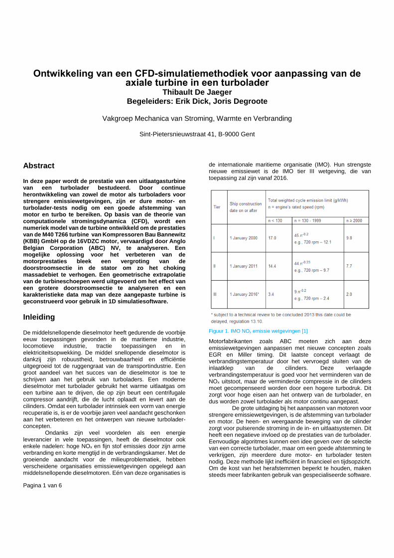
International Maritime Organization (IMO). Their most stringent new emission legislation is the IMO Tier III legislation, which will come into effect in 2016.
Figure 1. IMO NOx emission legislations [1]
Engine manufacturers like Anglo Belgian Corporation (ABC) NV have to respond to these emission legislations with new concepts such as Exhaust Gas Recirculation (EGR) and Miller timing. Miller timing lowers the combustion temperature by changing the intake valve close (IVC) time. The lowered combustion temperature is beneficial for NOx emissions, but implies a shortened compression stroke in the cylinder. This loss in compression has to be compensated by a higher boost pressure delivered by a turbocharger. This poses high demands on the turbocharger design, and requires re-development of both turbocharger and engine.
A constraint posed on the re-development of engines for more stringent emission legislations is the difficult matching between the turbocharger and the engine. The reciprocating motion of the cylinders results in pulsating flow in intake and exhaust systems, which is detrimental to the turbocharger performance. Simple algorithms, like the algorithm that KBB uses for the matching of turbochargers, can give an idea towards the selection of an appropriate turbocharger, but in order to achieve a good match, multiple expensive engine tests

Page 2 of 6
and turbocharger tests have to be performed. With the constantly changing emission legislations, this method seems inefficient time- and money-wise. In order to reduce costs of this re-matching, many manufacturers have been leaning towards specialist software. One dimensional engine simulation software like GT-Power, commercially available at Gamma Technologies, allow for analysis of a wide range of parameters and phenomena related to engine performance, while three dimensional Computational Fluid Dynamics (CFD) software like Fluent and CFX, both commercially available at ANSYS Inc., allow for analysis of the fluid flow in the engine components.
The object of this thesis is the T266 axial exhaust gas turbine of the M40 turbocharger from KompressorenBau Bannewitz (KBB) GmbH, of which two are placed on the 16VDZC engine from ABC. During an engine test performed in May 2013, it was found that the performance of the engine was not sufficient. Some important parameters from this engine test are given in the table below.
Table 1. Experimental test data for engine operating point 100%
Engine Load 100%
Engine Speed 1000 rpm
Mechanical Power 3400 kW
Specific Fuel Consumption 214.6 g/kWh
Specific Air Consumption 9.03 kg/kWh
Static Compressor Pressure Ratio 3.838
Total-to-Static Turbine Pressure Ratio 3.31
The goal of this dissertation is to provide ABC and KBB with a roadmap to improving the turbine design and its match with the 16VDZC engine short term. With the use of CFD software (CFX) the turbine characteristics are analysed and a proper possible solution is proposed. A second, more long-term envisioned, goal is to develop a simulation methodology for determining the turbine characteristics, and construct a data map of the axial turbine for the use in 1D-engine simulation software like GT-Power, and thus providing an alternative to expensive engine and turbocharger tests.
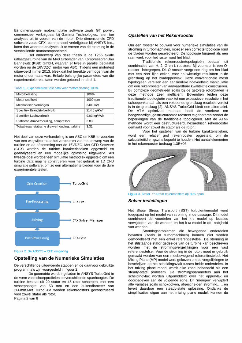
Figure 2. The ANSYS – CFD environment
Pre-processing
The steps performed and the software used are presented in Figure 2. The geometry is imported in ANSYS TurboGrid as blade profiles at different span locations. The turbine consists of 20 stator blades and 45 rotor blades, with a blade height 53mm and outside diameter 266mm. With TurboGrid, the grid is constructed separately for stator and rotor. The pre-processing is then performed in ANSYS CFX-pre
Grid Generation
In order to construct a grid for numerical simulations of the flow in turbo machinery, a correct topology around the blades has to be selected. The topology acts as a framework for the grid around the blade.
Traditional grid topologies consist of combinations of H,J,G and L grids. Preferably an O-grid is included. This O-grid adds a ring around the blade with a very fine mesh, for accurate boundary layer results on the blade surface. These conventional mesh topologies typically require a substantial amount of user manipulation to construct a grid of acceptable quality. With complex blade geometries like torsioned rotor blades, this method of meshing is very inefficient. Furthermore, these traditional topologies often result in an excessive mesh resolution within the blade passage when a sufficient boundary layer resolution is required [2]. ANSYS TurboGrid provides an alternative. The Automatic Topology and Meshing (ATM) optimized topology method is preferred to generate high-quality, structured grids without the constraints of the traditional topologies. With the ATM method a structured, hexahedral mesh is created separately for the stator and the rotor.
For the generation of turbine characteristics, a relatively coarse mesh for a single blade passage is constructed, in order to create a data map of a turbine in a reasonable timespan. This mesh has a number of cells of 1.3E+06.
Figure 3. Stator and Rotor Grid at 50% span
Solver Settings
The Shear Stress Transport (SST) turbulence model was applied to model the flow in the blade passage. This model combines the advantages of the k-ε model away from the walls and the k-ω model near the walls.
Flow problems that involve moving parts (as in turbomachinery) cannot be modelled with one reference frame. The geometry consists of two fluid zones, stator and rotor, with an interface boundary separating the zones. The stationary zone can be solved with the stationary frame equations, whereas the rotational section of the geometry can be solved using moving reference frame equations. The mixing plane

Page 3 of 6
approach was used to treat these equations at the interface. In the mixing plane model each fluid zone is treated as a steady-state problem. Flow-field data from the zones are passed as boundary conditions that are spatially averaged at the mixing plane interface. This mixing removes any unsteadiness due to circumferential variations in the passage-to-passage flow field ( wakes, shock waves, separated flow), therefore yielding a steady-state result. Despite the simplifications inherent in the mixing plane model, the results can provide reasonable approximations of the time-averaged flow field. Another option is the Sliding Mesh model (SM). The Sliding Mesh method models the relative motion of the two zones, where the rotor position is adjusted with every time step. This method is more accurate than a MP model but it is more computationally intensive.
As boundary conditions, the rotor speed, total inlet pressure, static outlet pressure and total inlet temperature were specified. The flow direction at the inlet is normal to the boundary, and the transported turbulence quantities at the inlet is defined by a turbulence intensity of 5% and a turbulence length scale of 0.038 ∗ 𝑑ℎ, where 𝑑ℎ is the hydraulic diameter at
the inlet (𝑑𝑜 − 𝑑𝑖).
The fluid flowing through the turbine is the cylinder exhaust gas. As an approximation, the fluid data from air was used. This is a good approximation because of the high air to fuel ratio in a diesel engine. However, due to the high exhaust temperature, the specific heat capacity Cp of the gas is adjusted to 1120 J/kgK. This is a value commonly used for exhaust gasses and was recommended by KBB.
Validation
Grid Independence
In order to analyse the influence of mesh size on the results, a grid independence study is executed with 4 different grids. Each grid is constructed with the same topologies for both the stator and the rotor section, but with coarser parameters. For each grid the calculation is executed with inlet conditions corresponding to the measured data from the ABC engine test at 100% engine load. The influence of the number of nodes on the mass flow rate and the effective turbine efficiency is shown in Figure 4. This graph shows that if the amount of cells is higher than 1.3 million, the difference in the properties displayed are negligible. It is then safe to assume that 1.3 million is the correct choice. For a higher amount of cells the increase in calculation time outweighs the small increase in accuracy.
Table 2. Grid numbers and some mesh parameters
Nr of cells grid 1 grid 2 grid 3 grid 4
Stator 391680 538110 716000 1153200
Rotor 370168 414494 580404 955264
total 761848 952604 1296404 2108464
Span wise 80 90 100 120
Shroud tip 10 12 14 18
Size factor 1 1.1 1.2 1.4
Min. y+ 2.75E-01 2.72E-01 2.69E-01 1.42E-01
Max. y+ 3.89E+01 2.93E+01 2.58E+01 7.24E+00
Figure 4. Grid independence test
Validation with Experimental Data
In order to validate the CFD calculations, experimental values are provided by KBB of the turbine. These were provided as a data map. The data is experimentally determined on a turbocharger test bed, and contains four performance parameters of the turbine: reduced speed, reduced mass flow rate, total-to-static pressure ratio, turbine effective efficiency and total inlet temperature. The reduced speed and reduced mass flow rates are calculated by:
𝑛𝑟𝑒𝑑𝑢𝑐𝑒𝑑 = 𝑛𝑎𝑐𝑡𝑢𝑎𝑙 √𝑇00 ⁄ [𝑟𝑝𝑚/√𝐾]
��𝑟𝑒𝑑𝑢𝑐𝑒𝑑 = ��𝑎𝑐𝑡𝑢𝑎𝑙
√𝑇00
𝑝00
[𝑘𝑔
𝑠∗
√𝐾
𝑘𝑃𝑎]
The effective turbine efficiency is calculated as:
𝜂𝑒𝑇 = 𝜂0,𝑖𝑠𝑇 ∗ 𝜂𝑚 = 𝜂0,𝑖𝑠𝑇 ∗ 0.97
Where 𝜂0,𝑖𝑠𝑇 is the total-to-static isentropic turbine efficiency.
The mechanical efficiency 𝜂𝑚 consists mainly of bearing and
friction losses (all mechanical losses in a turbocharger are attributed to the turbine side). Figure 5 and Figure 6 show the comparison between the experimental results and the numerical results obtained from the CFD computations. It is clear from these figures that the CFD calculated results are close to the experimental values. The maximum difference is 3.1% for the efficiency. CFD calculated mass flow rates are higher than the experimental values and the average difference between experimental and numerical values is 7.8%. An exact cause for this difference in mass flow rate is unknown, but it is probably due to slightly different properties of the fluid. A higher mass flow rate compared to experimental data is not uncommon for steady flow simulations for exhaust gas turbines [3].

Page 4 of 6
Figure 5. Comparison of CFX calculated efficiencies to experimental values
Figure 6. Comparison of CFX calculated mass flow rates to experimental values
Numerical Simulations with Engine Test Data
The input data for engine operating points was derived from an experimental engine test and are shown in table 3.
Table 4. CFX input data derived from experimental engine test
Load % 75 90 100 100+
Engine Speed rpm 1000 1000 1000 1000
Power kW 2550 3060 3400 3621
��𝑒𝑥ℎ kg/s 3.87 4.27 4.47 4.56
Turbo Speed rpm 31261 33520 35419 36520
p00 kPa 284 316 343 358
p2 kPa 103 103 104 104
T00 K 726 766 806 846
For every engine load point, a CFX numerical simulation was executed and the resulting turbine efficiencies are plotted on the acquired efficiency characteristic in Figure 7. The efficiency is decreasing for increased engine load, while the pressure ratio is increasing. The turbine is then not working at optimal efficiency for the engine maximum load. For marine diesel engines, this is not an uncommon observation, since the turbocharger needs high efficiency at lower loads as well. The higher turbocharger efficiencies at lower loads then result in a slightly deteriorated efficiency at maximum load. However, for an engine used for power generation applications like the 16VDZC, a high efficiency is needed at maximum load, and the efficiency at lower loads is of less importance.
Figure 7. Turbine efficiencies for engine operating points plotted on the efficiency curve
The turbine operating point for 100% engine load is situated at a high pressure ratio for the turbine. A comparison with the operating point of the turbine on the ABC 8DZC engine learns that the pressure ratio for the 16VDZC engine at 100% load is 3.31, and for the 8DZC engine this is 2.86, thus the 16VDZC engine has a higher inlet pressure for the turbine. Small differences between these engines might be expected due to the different construction of exhaust manifolds, but nevertheless, this indicates that the stator flow area (100cm²) for the turbine is too small. As a result from the high pressure ratios, the operating point of the turbine is close to choking conditions, which results in a lowered efficiency. Choking means that the flow reaches sonic state in a blade passage and may occur at high pressure ratios in either the stator or the rotor. For a turbine with low degree of reaction, choking occurs primarily in the stator. The choking mass flow rate is independent of rotational speed. The corresponding stator pressure ratio and mass flow rate are [4]:
𝑝1
𝑝01
= [ℎ1
ℎ01
]
𝑛𝑛−1⁄
= [2
𝛾 + 1]
𝑛𝑛−1⁄
��𝑐 = 𝐴1𝜌01𝑐01 [ℎ1
ℎ01
]
1𝑛−1
+12
Where n=2.32 is the polytropic exponent and 𝛾=1.4, the ratio of
specific heat capacities. With the numerical results it is calculated that the mass flow rate for choking in the stator is 4.606 kg/s. Similarly for the rotor [4]:
𝑝1
𝑝01
= [ℎ2
ℎ01
]
𝑛𝑛−1⁄
��𝑐 = 𝐴2𝜌01𝑐01 [ℎ2
ℎ01
]
1𝑛−1
+12
The mass flow rate for choking in the rotor is 6.209kg/s. It is clear that due to the turbine’s relative low degree of reaction, the stator is more prone to choking. The typical curve for mass flow rate as a function of total pressure ratio is provided in Figure 8 [4]. At 100% engine load, the average mass flow rate through the exhaust gas turbine is 4.47kg/s, which is very close to the “maximum” mass flow rate (choking mass flow rate) of the turbine.

Page 5 of 6
Figure 8. Mass flow rate in function of pressure ratio for choking in the stator [4]
Mass Flow Choking in the Stator
In order to understand why the efficiency is decreasing for pressure ratios above 2.7 (see figure 7), a flow analysis of the stator is executed for different pressure ratios. For this CFD analysis, the flow fields in the stator are numerically calculated with a different mesh then before. The grid independence test indicated that the mesh was accurate for calculating the properties in the previous section, but in order to accurately describe the flow near boundary layers, lower y+ values are required. This was not achieved in the previous numerical simulations, in order to keep calculation time reasonable. With a similar methodology, but a fine mesh (min. y+ 8.388E-02, max. y+ 1.102E00) the flow fields in the stator are analysed for different pressure ratios. The most important figures of this analysis are presented here.
Figure 9. Mach number distribution in the stator for a total-to-static pressure ratio of 2.824. The minimum Mach number in this figure is set to 0.6, to be able to distinguish the supersonic zone better
A pressure ratio of 2.824 is just greater than the pressure ratio at which maximum in the best fitted efficiency curve is expected. Figure 9 shows the Mach number and pressure plots of the flow field. Around this pressure ratio, the flow field alters from being entirely subsonic, and at the suction side of the vane, sonic speed is reached in one point. With increasing pressure ratios, this point grows into a supersonic zone, ending in a normal shock. The supersonic zone is influenced by the interaction with
the trailing edge of the neighbouring blade. After the normal shock, the boundary layer becomes wider. The normal shock at the end of the supersonic zone at the suction side, results in shock losses and due to small radial differences in the shock intensities, strongly rotational flow. This all leads to a decrease of the turbine efficiency.
At a total-to-static pressure ratio of 3.8, the flow reaches sonic speed at the throat section between the suction side of the blade and the trailing edge of the neighbouring blade. At this point, the outlet velocity of the stator is supersonic. In the flow field, the large supersonic zone is visible, with a strong, normal shock at the end. The wake flow of the neighbouring blade is again very influential on the shape of this supersonic zone.
Figure 10. Mach number distribution in the stator for a total-to-static pressure ratio of 3.8.
Figure 11. Mach number distribution in the stator for a total-to-static pressure ratio of 5.

Page 6 of 6
The normal shock hits the boundary layer of the suction side of the blade. The interaction with the boundary layer creates a lambda shaped bifurcation. Due to the impinging shock, the boundary layer becomes wider and the shock deflects somewhat (the shock is normal to the flow). Because of the concave curvature of the flow before the shock, compression waves are generated, that converge in the first leg of the lambda-shock. The convex curvature of the flow after the shock results in an expansion, with a small supersonic zone after the shock wave.
Figure 11 shows the flow field in the stator at a high total-to-static pressure ratio of 5 across the turbine. The flow field at such a high pressure ratio is rather complex. The supersonic zone as seen in at lower pressure ratios, has reached the trailing edge of the blade, and is very distorted. Two oblique shocks depart from the trailing edge of the blade. One of those shocks hits the suction side boundary layer of the blade. Because of the impinging oblique shock, the boundary layer becomes wider. The shock reflects on the sonic line in the boundary layer.
Design Adjustment of the Axial Turbine
In order to increase the choking mass flow rate, the simplest option is to increase the outside diameter of the turbine, and thus increasing the stator flow area. Other options included rotating of the stator vanes and removing one or more stator vanes. The option of increasing the outside diameter was chosen in order to lower the axial velocity and thus the stator outlet velocity, while not lowering the rotor speed too much. The outside diameter of the turbine is increased to 276mm, allowing for an increase of stator flow area of 12%.
Results for the Adjusted Turbine
With the same methodology as before, numerical iterations are performed to analyse the performance of the adjusted turbine. Figure 12 shows a comparison between the efficiency curves for the adjusted turbine, and the “old” turbine, both experimental and numerical, and figure 13 shows the mass flow rates for both turbines.
Figure 12. Efficiencies for the adjusted and “old” turbine, in function of pressure ratio
The adjusted turbine has higher efficiency at high pressure ratios and overall higher mass flow rates. This result is in line with the goals set by adjusting the turbine. At a mass flow rate
associated with the 100% engine load for the tested engine, the expected pressure ratio is 2.96.
Figure 13. Mass flow rates for the adjusted and “old” turbine, in function of pressure ratio
Conclusions
The matching of turbochargers to engines is a difficult task, with the help of 3D simulations, a reasonably accurate data map (constructed with the data from figures 12 and 13) for the turbine can be constructed. This data map can be used in 1D CFD simulation software like GT Power to analyse its effects on the engine, and thus eliminating the need of expensive engine and turbocharger tests. For this case, it is expected that the increased flow area will lead to better performance of the engine. The lowered exhaust manifold pressure will increase the engine power. However, the adjustment of the turbine blades in this dissertation was made by extrapolation of the blade profiles provided for the T266 turbine. For better results, a detailed study should be executed on the design of the rotor blades. The methodology used for the CFD analysis of the turbine proved to be very good for reasonably fast generation of accurate turbine characteristics. TurboGrid allowed for a very fast generation of an appropriate grid, while the turbo mode in the CFX pre-processing software allowed for fast adjustment of inlet conditions.
References
1. International Maritime Organization, www.imo.org, Feb 2014
2. Häuser, J., Xia, Y. “Modern introduction to Grid Generation”, EPF Lausanne, 1996
3. Tabatabaei, H., Boroomand, M., Taeibi, R. M., “An investigation on turbocharger turbine performance parameters under inlet pulsating flow”, ASME Journal of Fluids Engineering, Vol. 134, 2012
4. Dick, E., “Gas turbines”, 2013
Pagina 1 van 6
Ontwikkeling van een CFD-simulatiemethodiek voor aanpassing van de axiale turbine in een turbolader
Thibault De Jaeger Begeleiders: Erik Dick, Joris Degroote
Vakgroep Mechanica van Stroming, Warmte en Verbranding
Sint-Pietersnieuwstraat 41, B-9000 Gent
Abstract
In deze paper wordt de prestatie van een uitlaatgasturbine van een turbolader bestudeerd. Door continue herontwikkeling van zowel de motor als turboladers voor strengere emissiewetgevingen, zijn er dure motor- en turbolader-tests nodig om een goede afstemming van motor en turbo te bereiken. Op basis van de theorie van computationele stromingsdynamica (CFD), wordt een numeriek model van de turbine ontwikkeld om de prestaties van de M40 T266 turbine van Kompressoren Bau Bannewitz (KBB) GmbH op de 16VDZC motor, vervaardigd door Anglo Belgian Corporation (ABC) NV, te analyseren. Een mogelijke oplossing voor het verbeteren van de motorprestaties bleek een vergroting van de doorstroomsectie in de stator om zo het choking massadebiet te verhogen. Een geometrische extrapolatie van de turbineschoepen werd uitgevoerd om het effect van een grotere doorstroomsectie te analyseren en een karakteristieke data map van deze aangepaste turbine is geconstrueerd voor gebruik in 1D simulatiesoftware.
Inleiding
De middelsnellopende dieselmotor heeft gedurende de voorbije eeuw toepassingen gevonden in de maritieme industrie, locomotieve industrie, tractie toepassingen en in elektriciteitsopwekking. De middel snellopende dieselmotor is dankzij zijn robuustheid, betrouwbaarheid en efficiëntie uitgegroeid tot de ruggengraat van de transportindustrie. Een groot aandeel van het succes van de dieselmotor is toe te schrijven aan het gebruik van turboladers. Een moderne dieselmotor met turbolader gebruikt het warme uitlaatgas om een turbine aan te drijven, die op zijn beurt een centrifugale compressor aandrijft, die de lucht oplaadt en levert aan de cilinders. Omdat een turbolader intrinsiek een vorm van energie recuperatie is, is er de voorbije jaren veel aandacht geschonken aan het verbeteren en het ontwerpen van nieuwe turbolader- concepten.
Ondanks zijn veel voordelen als een energie leverancier in vele toepassingen, heeft de dieselmotor ook enkele nadelen: hoge NOx en fijn stof emissies door zijn arme verbranding en korte mengtijd in de verbrandingskamer. Met de groeiende aandacht voor de milieuproblematiek, hebben verscheidene organisaties emissiewetgevingen opgelegd aan middelsnellopende dieselmotoren. Eén van deze organisaties is
de internationale maritieme organisatie (IMO). Hun strengste nieuwe emissiewet is de IMO tier III wetgeving, die van toepassing zal zijn vanaf 2016.
Figuur 1. IMO NOx emissie wetgevingen [1]
Motorfabrikanten zoals ABC moeten zich aan deze emissiewetgevingen aanpassen met nieuwe concepten zoals EGR en Miller timing. Dit laatste concept verlaagt de verbrandingstemperatuur door het vervroegd sluiten van de inlaatklep van de cilinders. Deze verlaagde verbrandingstemperatuur is goed voor het verminderen van de NOx uitstoot, maar de verminderde compressie in de cilinders moet gecompenseerd worden door een hogere turbodruk. Dit zorgt voor hoge eisen aan het ontwerp van de turbolader, en dus worden zowel turbolader als motor continu aangepast. De grote uitdaging bij het aanpassen van motoren voor strengere emissiewetgevingen, is de afstemming van turbolader en motor. De heen- en weergaande beweging van de cilinder zorgt voor pulserende stroming in de in- en uitlaatsystemen. Dit heeft een negatieve invloed op de prestaties van de turbolader. Eenvoudige algoritmes kunnen een idee geven over de selectie van een correcte turbolader, maar om een goede afstemming te verkrijgen, zijn meerdere dure motor- en turbolader testen nodig. Deze methode lijkt inefficiënt in financieel en tijdsopzicht. Om de kost van het herafstemmen beperkt te houden, maken steeds meer fabrikanten gebruik van gespecialiseerde software.
Pagina 2 van 6
Eéndimensionale motorsimulatie software zoals GT power, commercieel verkrijgbaar bij Gamma Technologies, laten toe analyses uit te voeren van de motor. Drie dimensionele CFD software zoals CFX, commercieel verkrijgbaar bij ANSYS Inc., laten dan weer toe analyses uit te voeren van de stroming in de verschillende motorcomponenten. Het onderwerp van deze thesis is de T266 axiale uitlaatgasturbine van de M40 turbolader van KompressorenBau Bannewitz (KBB) GmbH, waarvan er twee in parallel geplaatst worden op de 16VDZC motor van ABC. Tijdens een motortest uitgevoerd in mei 2013, bleek dat het bereikte vermogen van de motor ondermaats was. Enkele belangrijke parameters van die experimentele resultaten worden getoond in tabel 1.
Tabel 1. Experimentele test data voor motorbelasting 100%
Motorbelasting 100%
Motor snelheid 1000 rpm
Mechanisch Vermogen 3400 kW
Specifiek Brandstofverbruik 214.6 g/kWh
Specifiek Luchtverbruik 9.03 kg/kWh
Statische drukverhouding, compressor 3.838
Totaal-naar-statische drukverhouding, turbine 3.31
Het doel van deze verhandeling is om ABC en KBB te voorzien van een wegwijzer naar het verbeteren van het ontwerp van de turbine en de afstemming met de 16VDZC. Met CFD Software (CFX) worden de turbine karakteristieken opgesteld en geanalyseerd en een mogelijke oplossing uitgewerkt. Als tweede doel wordt er een simulatie methodiek opgesteld om een turbine data map te construeren voor het gebruik in 1D CFD simulatie software, om zo een alternatief te bieden voor de dure experimentele testen.
Figuur 2. De ANSYS – CFD omgeving
Opstelling van de Numerieke Simulaties
De verschillende uitgevoerde stappen en de daarvoor gebruikte programma’s zijn voorgesteld in figuur 2. De geometrie wordt ingeladen in ANSYS TurboGrid in de vorm van schoepprofielen op verschillende spanhoogtes. De turbine bestaat uit 20 stator en 45 rotor schoepen, met een schoephoogte van 53 mm en een buitendiameter van 266mm.Met TurboGrid worden rekenroosters geconstrueerd voor zowel stator als rotor.
Opstellen van het Rekenrooster
Om een rooster te bouwen voor numerieke simulaties van de stroming in turbomachines, moet er een correcte topologie rond de bladen worden geselecteerd. De topologie fungeert als een raamwerk voor het raster rond het blad.
Traditionele rekenroostertopologieën bestaan uit combinaties van H, J, G en L roosters. Bij voorkeur is een O-rooster inbegrepen. Dit O-rooster voegt een ring om het blad met een zeer fijne cellen, voor nauwkeurige resultaten in de grenslaag op het bladoppervlak. Deze conventionele mesh typologieën vereisen een aanzienlijke hoeveelheid manipulatie om een rekenrooster van aanvaardbare kwaliteit te construeren. Bij complexe geometrieën zoals bij de getorste rotorbladen is deze methode zeer inefficiënt. Bovendien leiden deze traditionele topologieën vaak tot een excessieve resolutie in het schoepenkanaal als een voldoende grenslaag resolutie vereist is in de grenslaag [2]. ANSYS TurboGrid biedt een alternatief. De ATM optimized methode heeft de voorkeur om hoogwaardige, gestructureerde roosters te genereren zonder de beperkingen van de traditionele topologieën. Met de ATM-methode wordt een gestructureerd, hexaedrisch rekenrooster gemaakt voor zowel de stator als de rotor.
Voor het opstellen van de turbine karakteristieken, word een relatief grof rekenrooster opgesteld, om de calculatietijd enigszins beperkt te houden. Het aantal elementen in het rekenrooster bedraag 1.3E+06.
Figuur 3. Stator en Rotor rekenroosters op 50% span
Solver instellingen
Het Shear Stress Transport (SST) turbulentiemodel werd toegepast op het model van stroming in de passage. Dit model combineert de voordelen van het k-ε model op locaties verwijderen van de wanden en het k-ω model in de nabijheid van wanden. Stromingsproblemen die bewegende onderdelen bevatten (zoals in turbomachines) kunnen niet worden gemodelleerd met één enkel referentiestelsel. De stroming in het stilstaande stator gedeelde van de turbine kan beschreven worden met de stromingsvergelijkingen voor een vast referentiestelsel. Voor de stroming in de rotor, moet er gebruik gemaakt worden van een meebewegend referentiestelsel. Het Mixing Plane (MP) model werd gekozen om de vergelijkingen te beschrijven op het scheidingsvlak tussen beide onderdelen. In het mixing plane model wordt elke zone behandeld als een steady-state probleem. De stromingsparameters aan het scheidingvlak worden uitgemiddeld over het oppervlak en doorgegeven aan de volgende zone. Dit “mengen” verwijdert alle variaties zoals schokgolven, afgescheiden stroming,…, en levert daardoor een steady-state oplossing. Ondanks de simplificaties eigen aan het mixing plane model, kunnen de

Pagina 3 van 6
resultaten goede benaderingen van het tijds-gemiddelde stromingsveld opleveren. Een andere mogelijke optie is het Sliding Mesh model (SM). In dit model wordt de relatieve beweging van de twee zones gemodelleerd en wordt de positie van de rotor aangepast met elke tijdstap. Deze methode is nauwkeuriger dan het mixing plane model, maar vraagt meer rekenkracht.
De randvoorwaarden die gespecifieerd moesten worden waren: de rotor snelheid, de totale inlaatdruk, de statische uitlaatdruk en de totale inlaattemperatuur. De stroming wordt ingegeven als normaal aan het inlaatvlak, met een aanwezige turbulentie intensiteit van 5% en een turbulentie lengteschaal van 0.038 ∗ 𝑑ℎ, met 𝑑ℎ de hydraulische diameter
aan de inlaat (𝑑𝑜 − 𝑑𝑖).
Het fluïdum dat door de turbine stroomt is het uitlaatgas van de cilinders. De eigenschappen van lucht werden gebruikt met een aangepaste specifieke warmtecapaciteit Cp=1120J/kgK om het uitlaatgas te benaderen. Deze waarde van warmtecapaciteit wordt vaak gebruikt voor het beschrijven van uitlaatgassen en werd aangeraden door KBB.
Validatie
Rekenrooster onafhankelijkheid
Om de invloed van het rekenrooster op de resultaten na te gaan, werd een “grid independence test” uitgevoerd door middel van 4 verschillende rekenroosters. Elk rekenrooster is opgesteld met dezelfde topologieën, maar met grovere of fijnere parameters. Voor elk rekenrooster werd een numerieke simulatie uitgevoerd met inlaatcondities corresponderend met de bemeten data van de experimentele motortest aan 100% motorbelasting. De resultaten van de test zijn getoond in figuur 4.
Tabel. Grootte van de rekenroosters en enkele parameters
# Elements grid 1 grid 2 grid 3 grid 4
Stator 391680 538110 716000 1153200
Rotor 370168 414494 580404 955264
total 761848 952604 1296404 2108464
Span wise 80 90 100 120
Shroud tip 10 12 14 18
Size factor 1 1.1 1.2 1.4
Min. y+ 2.75E-01 2.72E-01 2.69E-01 1.42E-01
Max. y+ 3.89E+01 2.93E+01 2.58E+01 7.24E+00
Figuur 4. Grid independence test
Validatie met experimentele data
Om de resultaten van de CFD simulaties te valideren, werden er experimentele data voorzien onder de vorm van een SAE data map. Deze data werd experimenteel bepaald op een turbolader proefbank, en bevat vier prestatieparameters van de turbine voor meerdere werkingspunten: de gereduceerde snelheid, het gereduceerde massadebiet, totaal-naar-statisch drukverhouding en effectief rendement en de totale inlaattemperatuur. De gereduceerde waarden van snelheid en massadebiet worden bepaald door:
𝑛𝑟𝑒𝑑𝑢𝑐𝑒𝑑 = 𝑛𝑎𝑐𝑡𝑢𝑎𝑙 √𝑇00 ⁄ [𝑟𝑝𝑚/√𝐾]
��𝑟𝑒𝑑𝑢𝑐𝑒𝑑 = ��𝑎𝑐𝑡𝑢𝑎𝑙
√𝑇00
𝑝00
[𝑘𝑔
𝑠∗
√𝐾
𝑘𝑃𝑎]
Het effectieve turbine rendement worden berekend door:
𝜂𝑒𝑇 = 𝜂0,𝑖𝑠𝑇 ∗ 𝜂𝑚 = 𝜂0,𝑖𝑠𝑇 ∗ 0.97
Hier is 𝜂0,𝑖𝑠𝑇 het totaal-naar-statische isentropisch rendement.
Het mechanische rendement 𝜂𝑚 wordt vooral bepaald door
lager en wrijvingsverliezen (alle mechanische verliezen in een turbolader worden toegewezen aan de turbine). Figuur 5 en figuur 6 tonen de vergelijking tussen de experimentele resultaten en de numerieke resultaten. Het is duidelijk dat the resultaten verkregen door de numerieke iteraties heel dicht liggen bij de experimentele resultaten. Het maximale verschil in rendement is 3.1%. De verkregen massadebieten vertonen iets hogere waarden voor de numeriek simulaties, het gemiddelde verschil is 7.8%. Een precieze oorzaak voor dit verschil is niet geweten maar is waarschijnlijk te wijten aan het verschil tussen uitlaatgas en lucht. Een hoger massadebiet vergeleken met experimentele data komt vaker voor bij simulaties met stationaire stroming in uitlaatgasturbines [3].
Figuur 5. Vergelijking van experimentele rendementen met numerieke simulaties

Pagina 4 van 6
Figuur 6. Vergelijking van experimentele massadebieten met numerieke simulaties
Numerieke simulaties met motor test data
De inlaatcondities voor de numerieke simulaties worden afgeleid uit de experimentele data verkregen uit de motortest.
Tabel 4. CFX randvoorwaarden
Load % 75 90 100 100+
Engine Speed rpm 1000 1000 1000 1000
Power kW 2550 3060 3400 3621
��𝑒𝑥ℎ kg/s 3.87 4.27 4.47 4.56
Turbo Speed rpm 31261 33520 35419 36520
p00 kPa 284 316 343 358
p2 kPa 103 103 104 104
T00 K 726 766 806 846
Figuur 7. Effectieve rendementen voor motor werkingspunten, geplot op de rendement curve.
Voor elk werkingspunt van de motor werd een numerieke simulatie uitgevoerd en de resulterende effectieve turbine rendementen werden geplot op de turbine karakteristiek in figuur 7. Voor stijgende motorbelasting, daalt het rendement, en stijgt de drukverhouding. De turbine werkt niet aan optimaal rendement aan 100% motorbelasting. Voor marine dieselmotoren is dit niet ongewoon, aangezien de turbine ook een hoog rendement moet hebben bij lagere motorbelastingen. Om bij lagere motorbelastingen toch een redelijk rendement te verkrijgen, is het rendement bij 100% motorbelasting vaak iets later. De 16VDZC motor van ABC wordt echter vooral gebruikt in combinatie met een generator voor het opwekken van
elektriciteit. Voor die toepassing is een hoog rendement gevraagd aan maximale motorbelasting. Het rendement bij lagere belastingen is dan van minder belang.
Het werkingspunt van de turbine voor 100% motorbelasting ligt bij een hele hoge drukverhouding voor de turbine. Een vergelijking met het werkingspunt van de turbine op de ABC 8DZC motor leert dat de drukverhouding bij de 16VDZC 3.31 bedraagt, terwijl dit bij de 8DZC motor 2.86 bedraagt. Het ontwerp van de uitlaatcollectoren voor beide motoren is verschillend, maar toch kan men opmerken dat het verschil duidt op een statordoorstroomsectie (100cm²) die te klein is. Door de hoge drukverhouding, ligt het werkingspunt van de turbine heel dicht bij choking condities, wat resulteert in een verminderd rendement. Choking betekent dat de stromingen een sone snelheid behaalt in het stromingskanaal en kan bij hoge drukverhouding voorkomen in de stator of de rotor. Voor een turbine met lage reactiegraad, komt choking voor in de stator. Het massadebiet dat daarmee correspondeert is dan onafhankelijk van de rotorsnelheid. De corresponderende drukverhouding aan de uitlaat van de stator en het massadebiet zijn dan [4]:
𝑝1
𝑝01
= [ℎ1
ℎ01
]
𝑛𝑛−1⁄
= [2
𝛾 + 1]
𝑛𝑛−1⁄
��𝑐 = 𝐴1𝜌01𝑐01 [ℎ1
ℎ01
]
1𝑛−1
+12
Hier is n=2.32 de polytropische exponent en 𝛾=1.4, Het
berekende choking massadebiet bedraagt 4.606 kg/s. Een gelijkaardige berekening kan gedaan worden voor de rotor [4]:
𝑝1
𝑝01
= [ℎ2
ℎ01
]
𝑛𝑛−1⁄
��𝑐 = 𝐴2𝜌01𝑐01 [ℎ2
ℎ01
]
1𝑛−1
+12
Het massadebiet bij debietsblokkering (=choking) in de rotor is 6.209kg/s. Het is duidelijk dat door de lage reactiegraad van de turbine, de stator kritieker is voor debietsblokkering. De typische massadebietscurve in functie van drukverhouding wordt voorgesteld in figuur 8 [4]. Bij 100% motorbelasting bedraagt het massadebiet 4.47kg/s, wat heel dicht ligt bij het vooropgesteld choking massadebiet.
Figuur 8. Massadebiet in functie van drukverhouding bij debietblokkering in de stator [4]

Pagina 5 van 6
Debietsblokkering in de stator
Om beter te kunnen begrijpen waarom het rendement daalt voor drukverhoudingen boven 2.7 (zie figuur 7), werden stromingsanalyses uitgevoerd voor verschillende drukverhoudingen. Voor deze CFD-analyse werd het stromingsveld in de stator bepaald met een aangepast rekenrooster. De grid-onafhankelijkheid van het basis- rekenrooster werd aangetoond in een vorige sectie, maar de y+ waarden laten niet toen om een nauwkeurige analyse van de stroming in de buurt van grenslagen uit te voeren. Daarom werd een aangepast rekenrooster ontwikkeld met lage y+ waarden (min. y+ 8.388E-02, max. y+ 1.102E00). Lage y+ waarden waren niet beoogd voor het basisrekenrooster om de rekentijd te beperken. De belangrijkste figuren van deze analyse worden hier getoond (figuren 9, 10 en 11).
Figuur 9. Contourplot van het Mach getal in de stator sectie, bij drukverhouding 2.824. Het minimum Machgetal is aangepast in deze figuur naar 0.6, om de supersone zone beter aan te tonen.
Een drukverhouding van 2.824 is net groter dan de drukverhouding waarop het maximum van de best passende curve in figuur 7 wordt verwacht. Figuur 9 toont het stromingsbeeld aan de hand van het Machgetal in de stator- sectie. Rond deze drukverhouding, verandert het stromingsbeeld van volledig subsoon naar transsoon, doordat er op de zuigzijde in één punt de geluidsnelheid bereikt wordt. Dit punt groeit tot een supersone zone, die eindigt in een normale schokgolf. In te figuur is te zien dat deze supersone zone vervormd wordt door het zog van de volgende schoep in de schoepenrij. Door de interactie van de schokgolf met de grenslaag wordt de grenslaag breder. De normale schokgolf gaat gepaard met schokverliezen en door radiale variaties in schoksterkte ontstaat er een rotatie in de stroming. Dit leidt tot een vermindering van het turbinerendement. Bij een totaal-naar-statische drukverhouding van 3.8, bereikt de stroming in de keelsectie de geluidsnelheld en de supersone zone is aldus gegroeid en beslaat de hele sectie. In het stromingsbeeld is de grote supersone zone zichtbaar, met een sterke, normale schok aan het einde. Het zog van de naburige schoep is opnieuw nadrukkelijk aanwezig en vervormt de supersone zone.
De normale schokgolf raakt de grenslaag aan de zuigzijde van de schoep. De interactie van de grenslaag creëert een lambda-vormige bifurcatie. Door de invallende schok, verbreedt de grenslaag en de schok buigt af (de schokgolf blijft loodrecht op de grenslaag). Door de concave buiging van de grenslaag voor de schok, worden er compressiegolven gegenereerd, die convergeren in het eerste been van de lambda-schok. De convexe buiging na de schok resulteert in een expansie, met een kleine supersone zone na de schokgolf.
Figuur 10. Contourplot van het Mach getal in de stator sectie bij drukverhouding 3.8
Figuur 11. Contourplot van het Mach getal in de stator sectie bij drukverhouding 5
Figuur 11 toont het stromingsbeeld in de stator bij een hoge totaal-naar-statische drukverhouding van 5. Het stromingsbeeld is nu veel complexer. Twee schuine schokken vertrekken van de achterste rand van de schoep. Eén van die schokken valt in op de zuigzijde van de nabijgelegen schoep. De schok reflecteert op de sone lijn in de grenslaag.

Pagina 6 van 6
Aanpassing van de Axiale turbine
Er werd beslist dat om het massadebiet bij debietsblokkering te verhogen, de eenvoudigste oplossing was om de buitendiameter van de turbine te vergroten. Andere mogelijkheden waren o.a. het roteren van de statorschoepen of het verwijderen van een of meerdere schoepen. Een vergroting van de buitendiameter werd gekozen om zo de axiale stromingssnelheid en bijgevolg de statoruitlaatsnelheid te verminderen, zonder de rotorsnelheid te veel te doen verminderen. De buitendiameter is vergroot tot 276mm, zodat de doorstroomsectie van de stator vergroot wordt met 12%. Het ontwerp van het schoepenprofiel op die diameter werd afgeleid uit de andere profielen.
Resultaten voor de Aangepaste Turbine
Met dezelfde methodologie als voorheen, werden er numerieke iteraties uitgevoerd om de prestaties van de aangepaste turbine te analyseren. Figuur 12 toont een vergelijking van de rendementscurves voor beide turbines. Van de T266 turbine zijn zowel experimentele als numerieke data voorhanden. Figuur 13 toont het massadebiet in functie van de drukverhouding voor beide turbines.
De aangepaste turbine heeft een hoger rendement bij hoge drukverhouding en een hoger massadebiet. Dit resultaat is in lijn met de doelen gezet bij het aanpassen van de turbine. Bij een massadebiet geassocieerd met 100% belasting, is de verwachte drukverhouding 2.96.
Figuur 12. Rendementscurves in functie van drukverhouding vergeleken voor beide turbines
Figuur 13. Massadebiet in functie van drukverhouding voor beide turbines
Besluiten
Het afstemmen van turboladers aan motoren is een moeilijke taak. Met de hulp van 3D simulatietechnieken, kunnen de karakteristieken van de turbine met goede nauwkeurigheid bepaald worden. De data map die zo werd verkregen kan nu gebruikt worden in 1D CFD simulatie software zoals GT Power om het effect van de turbine op de motor beter te analyseren. In dit geval, is het te verwachten dat de grotere doorstroomsectie zal leiden tot een betere prestatie van de motor. De verlaagde druk in de uitlaatcollector zal zorgen voor betere motorprestaties. Om goede resultaten te halen, moet wel nog een correct ontwerp van turbinebladen bedacht worden, aangezien die in deze verhandeling geëxtrapoleerd werd uit het ontwerp van de turbine bladen voor de T266 turbine. De methodologie die gebruikt werd voor de CFD analyse van de turbine liet toen om in relatief korte tijd nauwkeurige karakteristieken op te stellen van de turbine. TurboGrid liet toe om snel een toepasselijk rekenrooster te construeren, terwijl de turbo mode in de CFX-pre software toeliet om de inlaatcondities aan te passen.
Referenties
1. International Maritime Organization, www.imo.org, Feb 2014
2. Häuser, J., Xia, Y. “Modern introduction to Grid Generation”, EPF Lausanne, 1996
3. Tabatabaei, H., Boroomand, M., Taeibi, R. M., “An investigation on turbocharger turbine performance parameters under inlet pulsating flow”, ASME Journal of Fluids Engineering, Vol. 134, 2012
4. Dick, E., “Gasturbines”, 2013

Preface
With this preface, I would like to take time and mention everyone I am grateful to for helping
me with the realization of this dissertation.
In the first place, I would like to thank prof. Dr. Ir. Erik Dick for sharing his expertise and
experience and for his guidance in accomplishing this thesis. I was always able to rely on his
support. I would also like to thank prof. Dr. Ir. Joris Degroote for his valuable assistance.
Next to the people supporting me at the Ghent University, I have to express my gratitude to
the technical staff at ABC, for my welcome reception at their company and in particular to
Ir. Lieven Vervaeke for allowing me to work on this topic and for his confidence and interest
in my research. The technical staff from KBB deserve a word of thanks as well for their
welcome reception of me at their offices in Bannewitz.
This word of gratitude would not be complete without thanking my parents and siblings for
their unconditional support during my 5 years study at the Ghent University. Without them
I would certainly not have been at this point in my life. To conclude this preface, I would
also like to thank my friends and especially Evi. Thanks to them, I can look back joyfully to
the past five years, and be hopeful for what the future brings.
Thibault De Jaeger
Ghent, June 2014
i

Contents
Preface i
List of symbols iv
1 Introduction 1
1.1 General Introduction . . . . . . . . . . . . . . . . . . . . . . . . . . . . . . . . 1
1.2 Turbocharger Developments . . . . . . . . . . . . . . . . . . . . . . . . . . . . 4
1.2.1 Charge Air Compressor Design Optimization . . . . . . . . . . . . . . 4
1.2.2 Exhaust Gas Turbine Design Optimization . . . . . . . . . . . . . . . 8
1.2.3 Alternative Turbocharger Configurations . . . . . . . . . . . . . . . . . 13
2 Numerical Methods 19
2.1 Introduction . . . . . . . . . . . . . . . . . . . . . . . . . . . . . . . . . . . . . 19
2.2 Theory of Computational Fluid dynamics . . . . . . . . . . . . . . . . . . . . 19
2.2.1 Governing Equations . . . . . . . . . . . . . . . . . . . . . . . . . . . . 19
2.2.2 Turbulence modelling . . . . . . . . . . . . . . . . . . . . . . . . . . . 20
2.2.3 Flow in Multiple Reference Frames . . . . . . . . . . . . . . . . . . . . 21
2.3 Validation of CFD results . . . . . . . . . . . . . . . . . . . . . . . . . . . . . 22
3 Pre-processing for CFD Analysis 24
3.1 Introduction . . . . . . . . . . . . . . . . . . . . . . . . . . . . . . . . . . . . . 24
3.2 Geometry Definition . . . . . . . . . . . . . . . . . . . . . . . . . . . . . . . . 25
3.3 Meshing of Turbine blades . . . . . . . . . . . . . . . . . . . . . . . . . . . . . 28
3.3.1 Grid Topology . . . . . . . . . . . . . . . . . . . . . . . . . . . . . . . 29
3.3.2 Stator Grid . . . . . . . . . . . . . . . . . . . . . . . . . . . . . . . . . 29
3.3.3 Rotor Grid . . . . . . . . . . . . . . . . . . . . . . . . . . . . . . . . . 31
3.4 CFX-Pre Settings . . . . . . . . . . . . . . . . . . . . . . . . . . . . . . . . . . 34
3.4.1 Fluid Definition . . . . . . . . . . . . . . . . . . . . . . . . . . . . . . . 34
3.4.2 Boundary Conditions . . . . . . . . . . . . . . . . . . . . . . . . . . . 34
3.4.3 Solver Settings . . . . . . . . . . . . . . . . . . . . . . . . . . . . . . . 36
4 Validation 37
4.1 Grid Validation . . . . . . . . . . . . . . . . . . . . . . . . . . . . . . . . . . . 37
ii

Contents iii
4.1.1 Grid Independence Test . . . . . . . . . . . . . . . . . . . . . . . . . . 37
4.1.2 y+ Values . . . . . . . . . . . . . . . . . . . . . . . . . . . . . . . . . . 38
4.2 Validation with Experimental Values . . . . . . . . . . . . . . . . . . . . . . . 39
4.2.1 Experimental Data . . . . . . . . . . . . . . . . . . . . . . . . . . . . . 39
4.2.2 Efficiency Calculations . . . . . . . . . . . . . . . . . . . . . . . . . . . 40
4.2.3 Results . . . . . . . . . . . . . . . . . . . . . . . . . . . . . . . . . . . 41
5 Analysis of the Results 43
5.1 Introduction . . . . . . . . . . . . . . . . . . . . . . . . . . . . . . . . . . . . . 43
5.2 Results . . . . . . . . . . . . . . . . . . . . . . . . . . . . . . . . . . . . . . . . 44
5.2.1 Turbine Efficiency . . . . . . . . . . . . . . . . . . . . . . . . . . . . . 44
5.2.2 Mass Flow Rate . . . . . . . . . . . . . . . . . . . . . . . . . . . . . . 44
5.2.3 Velocity Triangles and Kinematic Parameters . . . . . . . . . . . . . . 44
5.2.4 Torque and Power . . . . . . . . . . . . . . . . . . . . . . . . . . . . . 46
5.2.5 Blade Loading . . . . . . . . . . . . . . . . . . . . . . . . . . . . . . . 48
5.2.6 Analysis of the Flow at 100% Engine Load . . . . . . . . . . . . . . . 49
5.3 Turbine Mass Flow Choking . . . . . . . . . . . . . . . . . . . . . . . . . . . . 52
5.4 Stator Analysis . . . . . . . . . . . . . . . . . . . . . . . . . . . . . . . . . . . 54
5.5 Rotor Analysis . . . . . . . . . . . . . . . . . . . . . . . . . . . . . . . . . . . 59
6 Axial Turbine Geometry Adjustment 64
6.1 Introduction . . . . . . . . . . . . . . . . . . . . . . . . . . . . . . . . . . . . . 64
6.2 Adjustment Method . . . . . . . . . . . . . . . . . . . . . . . . . . . . . . . . 66
6.2.1 Adjusting the Stator . . . . . . . . . . . . . . . . . . . . . . . . . . . . 66
6.2.2 Adjusting the Rotor . . . . . . . . . . . . . . . . . . . . . . . . . . . . 67
7 Results 69
7.1 Introduction . . . . . . . . . . . . . . . . . . . . . . . . . . . . . . . . . . . . . 69
7.2 SAE Data map . . . . . . . . . . . . . . . . . . . . . . . . . . . . . . . . . . . 69
7.3 Performance Analysis . . . . . . . . . . . . . . . . . . . . . . . . . . . . . . . 73
8 Conclusions and Recommendations 74
A SAE data maps 76
B Stator Mesh for flow analysis 79
C Compressor Data map 82
Bibliography 84
List of Figures 87
List of Tables 90

List of symbols
Symbol or Abbreviation Meaning
ABC Anglo Belgian Corporation NV
KBB KompressorenBau Bannewitz GmbH
NOx Nitrogen Oxides
PM Particulate matter
IMO International Maritime Organization
CFD Computational Fluid Dynamics
BMEP Break Mean Effective Pressure
SAE Society of Automotive Engineers
m Mass flow rate
T Temperature
p Pressure
π Pressure ratio
LP Low pressure
HP High pressure
t Time
ρ Density
~U Velocity vector~~τ Stress tensor
h Enthalpy
~SM Source term of momentum
µ Dynamic viscosity
µt Turbulent viscosity
ν Kinematic viscosity
~ω Angular velocity vector
~r Location vector
k Turbulent kinetic energy
ε Turbulent kinetic energy dissipation rate
iv

Chapter 0. List of symbols v
ω Specific dissipation rate
SST Shear Stress Transport
MRF Multiple Reference Frame
SM Sliding Mesh
MP Mixing Plane
η efficiency
cp Specific heat capacity
Cpg Specific heat capacity of exhaust gas
γ Ratio of specific heat capacities
ATM Automatic Topology and Meshing
D Diameter
dh Hydraulic diameter
do outer diameter
di inner diameter
R Gas constant
∆W Work
P Power
R Degree of Reaction
ϕ Flow coefficient
ψ Work coefficient
u Rotor velocity
v Flow velocity
w Relative flow velocity
α Flow angle
β Relative flow angle
c sonic speed
A Area
n Polytropic exponent

Chapter 0. List of symbols vi
Subscripts
in value at an inlet
out value at an outlet
00 Total value at inlet of turbine
01 Total value between stator and rotor
02 Total value at outlet of turbine
0 Value at inlet of turbine
1 Value between stator and rotor
2 Value at outlet of turbine
is Isentropic
T Turbine
C Compressor
exh Exhaust
eT Effective Turbine
ref Reference
a Axial
t Tangential
av Average
c Choking
tot-st Total-to-Static

Chapter 1
Introduction
1.1 General Introduction
For over a century, the medium speed diesel engine has found a widespread use in mar-
itime, locomotive, traction and power generation applications. Its reliability, efficiency and
robustness have made the medium speed diesel engine the backbone of the transport indus-
try today. One of the major features in achieving this success was the use of turbochargers.
A modern turbocharged engine uses the exhaust gas to spin a turbine, which drives a cen-
trifugal compressor to compress the ambient air and deliver it to the engine cylinders. A
high boost pressure provided by this compressor is required in order to improve the power
density, and specific fuel consumption. Because a turbocharger is intrinsically a form of en-
ergy recuperation, turbochargers play a big role in the race towards more efficient internal
combustion engines. And so, in recent years, special attention has been given to the devel-
opment and improvement of turbocharger systems. The greatest challenge for turbocharger
manufacturers is to increase the boost pressure, the turbocharger efficiency, and improve the
part load behaviour whilst still delivering the required power at full load.
Anglo Belgian Corporation nv or ABC is a medium speed diesel engine manufacturer located
in Ghent. ABC is manufacturing diesel engines since 1912. The company has the reputation
of building robust and simple engines, with low fuel and lubricating oil consumption, long
lifetime, low maintenance cost and easy accessibility. The engine power ranges from 300kW
for the DX series, up to 5200 kW for the new DL36 engines. Other engines in this range are
the DZ-series with 6 or 8 cylinders, and the VDZ-series with 12 or 16 cylinders in a V con-
figuration. Except for the naturally aspirated versions of the DX-series, all ABC engines are
equipped with turbochargers. These turbochargers are manufactured by Kompressorenbau
Bannewitz GmbH or KBB in Dresden, Germany. KBB was founded in 1948 and has been
active in the field of turbochargers since 1953. It manufactures turbochargers with axial-flow
and radial-flow turbines. Both ABC and KBB are part of the OGEPAR group.
1

Chapter 1. Introduction 2
As already mentioned, diesel engines have great advantages as energy providers in many
applications. However, the diesel engine has high nitrogen oxides (NOx) and Particulate
Matter (PM) emissions due to its lean operation and the short available mixing time in
the combustion chamber. With the increasing environmental awareness of the last decades,
several organisations have imposed emissions legislations for medium speed diesel engines.
One of those organisations is the International Maritime Organization (IMO). Their most
stringent new emission legislation is the IMO Tier III legislation (see Figure 1.1), which will
come into effect in 2016.
Figure 1.1: IMO NOx emission limitations [1]
Engine manufacturers like ABC have to respond to these emission legislations with new con-
cepts such as Exhaust Gas Recirculation (EGR) and Miller timing [2]. Miller timing lowers
the combustion temperature by changing the intake valve close (IVC) time. The lowered
combustion temperature is beneficial for NOx emissions, but this implies a shortened com-
pression stroke in the cylinder. This loss in compression has to be compensated by a higher
boost pressure delivered by a turbocharger. This poses high demands on the turbocharger
design, and requires redevelopment of both turbocharger and engine.
A constraint posed on the re-development of engines for more stringent emission legislations
is the difficult matching between the turbocharger and the engine. The reciprocating motion
of the cylinders results in pulsating flow in intake and exhaust systems, which is detrimental
to the turbocharger performance. Simple algorithms, like the algorithm that KBB uses
for matching turbochargers to various engine applications, can give an idea towards the
selection of an appropriate turbocharger, but in order to achieve a good match, multiple
expensive engine tests and turbocharger tests have to be performed. With the constantly
changing emission legislations, this method seems inefficient time- and moneywise. In order

Chapter 1. Introduction 3
to reduce costs of this re-matching, many manufacturers have been leaning towards specialist
software. One dimensional engine software like GT-Power, commercially available at Gamma
Technologies, allow for analysis of a wide range of parameters and phenomena related to
engine performance, while three dimensional Computational Fluid Dynamics (CFD) software
like Fluent and CFX, both commercially available at ANSYS Inc., allow for analysis of the
fluid flow in the engine components.
The object of this thesis is the T266 axial exhaust gas turbine of the M40 turbocharger from
KBB, of which two are placed on the 16VDZC engine from ABC. During an engine test
performed in May 2013, it was found that the performance of the engine was not sufficient.
While the 8DZC engine (with 8 cylinders) produces 2000 kW mechanical power at maximum
load, and the 12VDZC engine (with 12 cylinders in V configuration), produces 3000 kW, the
16VDZC engine produces no more than 3400 kW mechanical power at maximum load. A
closer comparison is provided in the table below.
Engine 8DZC 12VDZC 16VDZC
Turbocharger M40 2x M40 2x M40
Compressor C184B2 C170A C184B2
Turbine T266/4/100 T266/11/90 T266/9.5/100
Power (kW ) 2000 3000 3400
Engine Speed (rpm) 1000 1000 1000
Specific fuel consumption (g/kWh) 209.5 205.4 214.6
Volumetric flow rate per compressor (m3/s) 3.686 2.862 3.650
Specific air consumption (kg/kWh) 6.9387 7.447 9.03
πtot−st,T 2.862 - 3.310
πst−st,C 3.589 - 3.838
Table 1.1: Comparison between different engines
The results from the engine test performed, and a GT-power analysis in the summer of 2013,
raised presumptions that the suboptimal performance of the engine is due to the exhaust
gas turbine working at near-choking conditions, limiting the air flow through and thus the
performance of the engine, as well resulting in a turbocharger performing at a low efficiency.
The goal of this thesis is to provide ABC and KBB with a roadmap to improving the turbine
design and its match with the 16VDZC engine short term. With the use of CFD software
(CFX) the turbine characteristics are analysed and a proper possible solution is proposed.
A second, more long-term envisioned, goal is to develop a simulation methodology for deter-
mining the turbine characteristics, and construct a ‘SAE’- data map of the axial turbine for
the use in 1D-engine simulation software like GT-Power, and thus providing an alternative

Chapter 1. Introduction 4
to expensive engine and turbocharger tests.
For the remainder of this Chapter, a literature study is provided about recent turbocharger
developments. In Chapter 2, some numerical methods are discussed for performing 3D Com-
putational Fluid Dynamics simulations and this will conclude the entire literature study for
this dissertation. Upward of Chapter 3, the actual steps performed in this work are discussed.
Chapter 3 covers the set-up of the numerical simulations, with a description of the turbine
geometry and its implementation in Ansys TurboGrid, and the generation of the grid. In
Chapter 4 the generated grid is validated, and the results are analysed in Chapter 5. A pos-
sible way of solving the problem is provided in Chapter 6, and the results of this adjustment
are shown in Chapter 7. This dissertation finishes with Chapter 8, where the conclusions,
and some recommendations are formulated.
1.2 Turbocharger Developments
1.2.1 Charge Air Compressor Design Optimization
Optimization of turbocharger compressors is tended towards producing higher boost pressure
for the engine, whilst also improving turbocharger efficiency. By increasing the boost pressure,
engines can be built with higher Break Mean Effective Pressure (BMEP), and higher BMEP
results in more power produced with the same swept volume, resulting in a higher power
output [3]. In Figure 1.2 this relation is shown by the blue circles for medium speed engines
[4].
In medium speed diesel engines, the turbocharger compressor is almost exclusively con-
structed as an open radial type compressor with an inducer/impeller part with splitter blades,
followed by a vaned diffuser and a volute. So in the following sections, optimization techniques
on these components are discussed.
Chapter 1. Introduction 5
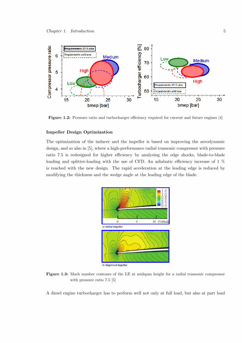
Figure 1.2: Pressure ratio and turbocharger efficiency required for current and future engines [4]
Impeller Design Optimization
The optimization of the inducer and the impeller is based on improving the aerodynamic
design, and so also in [5], where a high-performance radial transonic compressor with pressure
ratio 7.5 is redesigned for higher efficiency by analysing the edge shocks, blade-to-blade
loading and splitter-loading with the use of CFD. An adiabatic efficiency increase of 1 %
is reached with the new design. The rapid acceleration at the leading edge is reduced by
modifying the thickness and the wedge angle at the leading edge of the blade.
Figure 1.3: Mach number contours of the LE at midspan height for a radial transonic compressor
with pressure ratio 7.5 [5]
A diesel engine turbocharger has to perform well not only at full load, but also at part load

Chapter 1. Introduction 6
operation. This poses problems for the compressor, due to the occurrence of surge. The
reduced flow rate may result in rotating stall within the impeller or the vaned diffuser. This
generates losses, causing a decrease of the pressure ratio [6].
A possible solution for part load operation has been provided in [7], where a casing treatment
is used to accommodate a wider operating range to avoid surge. This casing treatment
consists of an upstream slot located in the compressor inlet, with a bleed slot downstream
with an annular cavity connecting the slots. When the pressure at the bleed slot is larger
than at the upstream slot, part of the flow will bypass the bleed slot and will recirculate
to the flow upstream of the impeller. When the volume flow is low, the pressure difference
between bleed and upstream slots is larger and the recirculation is stronger.
This recirculation results in an improved incidence at the leading edge of the impeller, so the
stall is suppressed and the operating range widens. In Figure 1.4 this casing treatment is
represented, while in Figure 1.5 the influence of such a casing treatment is shown by means
of a compressor map, where the red line represents the presence and the grey line the absence
of this casing treatment [8].
In Figure 1.6 [9], the pressure distribution at the compressor shroud is shown, demonstrating
the driving forces behind the recirculating flow. At near surge operating conditions, the
pressure difference between the downstream and the upstream slot forces the recirculation.
The flow rate through the inducer is then less prone to separation. At near choke operating
conditions, the pressure difference is negative, and part of the flow bypasses the inducer inlet.
The effect of this mechanism on the compressor characteristics is comparable to Figure 1.5.
Figure 1.4: recirculation device on a radial turbocharger compressor [7]

Chapter 1. Introduction 7
Figure 1.5: A compressor map showing the influence (red) of a compressor case treatment on the
surge limit [8]
Figure 1.6: pressure distribution at radial compressor shroud [9]
Vaned Diffuser Design Optimization
The diffuser tends to limit compressor performance, due to the complex impeller wake flows
that lead to regions of reversed flow at the diffuser inlet flows, coupled with dominant 3D

Chapter 1. Introduction 8
vortical flows in the diffuser passages. Siemens Industrial Turbomachinery (SIT) [10] discov-
ered that this secondary flow may result in an negative incidence towards 9 degrees at the
hub and up to 40 degrees at the shroud. This incidence will result in separated flow on both
the suction and the pressure side of the vane. In Figure 1.7 the streamlines show dominant,
counter-rotating vortical structures and reversed flow.
With a swept diffuser leading edge, the flow separation was overcome, and the compressor
characteristic found an improvement in width, and an improvement in peak total-to-static
efficiency of 1%. However, this advantage disappears at higher pressure ratios where the
performance is determined largely by the impeller. The swallowing capacity, m√T0,in/p0,in,
has a wider range, and the compressor map shows a wide region of high efficiency and high
peak efficiency.
Another method to decrease the tendency towards boundary separation is by adjusting the
diffuser vane leading edge from the traditional circular shape to an elliptic leading edge
(Figure 1.8), increasing the compressor efficiency by 0.2% [10]. By applying an elliptical
shape to the leading edge of the diffuser vane, the boundary layer is suppressed, diminishing
the tendency towards boundary separation.
In order to reduce swirl in the vaned compressor diffuser and strengthen the boundary layer
in the flow channels, PBS turbo [11] tested the possibility of introducing milled trajectories
in the diffuser (see figure 11). These milled trajectories have no influence on surge or choke
limits, but exert a small efficiency drop at lower pressure ratio.
Volute Design Optimization
Similarly to the diffuser, the volute has strong influences on the flow passing through the
impeller. An important parameter is the radial velocity at the volute inlet [12]. The radial
velocity is directly related to the swirl velocity in the volute, which is dissipated as a loss.
In order to decelerate the radial component of the flow velocity , an area expansion in both
the radial and axial directions has to be incorporated in the volute design. However, hub
separation is generated when the volute inlet is too large. Compressor manufacturers have
to carefully deliberate on the design of the centrifugal compressor volute to maximize the
compressor efficiency.
1.2.2 Exhaust Gas Turbine Design Optimization
A turbocharger turbine can be constructed as a radial turbine or an axial turbine. For medium
speed diesel engines the most common design is an axial turbine, but for high speed (smaller)
diesel engines the turbocharger turbine is exclusively constructed as a radial turbine, because

Chapter 1. Introduction 9
Figure 1.7: Streamlines at a vaned diffuser showing the complex secondary flow [10]
Figure 1.8: A circular leading edge (blue) and an elliptical leading edge (red) [10]
Figure 1.9: A polished (left), vs a milled (right) compressor diffuser [11]

Chapter 1. Introduction 10
of the small dimensions. The axial turbine of a medium speed diesel engine is constructed
by a nozzle ring with stator vanes, followed by a rotor, a diffuser and a collector.
Siemens Industrial Turbo machinery has developed a new type of collector for axial turbines
in turbochargers [10]. The collector is located downstream of the turbine diffuser and guides
the flow towards the exhaust. The flow in such a collectors show strong vortical structures
(streamlines are visible in Figure 1.10a). These strong velocity variations are due to the
strong difference in average flow velocity at the shroud and the hub. The velocity at the
shroud may be up to twice as high as at the hub.
These vortices in the collector cause severe losses and thus deteriorate the pressure reco-
very from the diffuser. By adding a collector neck splitter (Figure 1.10b) SIT managed to
increase the pressure recovery from the diffuser/collector combination with 11.5% and the
circumferential uniformity improved. Lower pressure gradients are clearly visible.
Special attention has to be made towards the vibrational behaviour of the turbine blades.
Due to the pulsating flow from the reciprocating cylinders, along with particulate matter
flowing through the turbine at high speeds, the rotor blades of an exhaust gas turbine are
prone to failures. Typical turbine failures are largely due to fatigue fractures and creep [13].
This means for exhaust gas turbines that there are a few contradictory design features. In
order to compensate for blade erosion, the rotor should be made out of thick blades, while high
efficiency requires thin blades. On top of that, resonance modes of the blades are located
dangerously close or even in the operating range of the turbocharger. This last condition
imposes careful design consideration. Companies like MAN B&W [14, 15], PBS Turbo [16]
and KBB [17] perform several vibration tests on new turbine blade designs in order to reduce
the probability of failure.
Variable Turbine Geometry
The design of a turbine is always matched to a specific optimal operating point. However, in
a turbocharger arrangement, the turbine rarely works at optimal conditions, and so, over the
years, research has been directed towards broadening the performance range of the turbine
in turbochargers.
The technology of variable stator vanes has been used extensively and with great success on
power gas turbines, and turbocharger manufacturers are now introducing this technology to
the nozzle ring vanes of exhaust gas turbines, both on axial and radial turbines. Figure 1.11
shows an axial exhaust gas turbine with adjustable stator vanes, constructed by ABB [18].
The rotation of the vanes is controlled by a lever. At low flow rates (low engine load), the
flow surface through the nozzle ring is reduced, increasing the turbine rotation speed and
thus the compressor delivers a higher boost pressure.

Chapter 1. Introduction 11
Figure 1.10: (a) Standard turbine outlet collector design with flow features; (b) improved turbine
outlet collector design [10]
Figure 1.11: Variable turbine geometry for axial turbines[18]

Chapter 1. Introduction 12
Adjustable stator vanes were also developed for radial turbines. Figure 1.12 shows such a
rotor cascade [19]. In this configuration, special attention has to be brought to the generation
of leakage flow. With the smallest opening of the nozzle, the leakage flow becomes dominant
in the flow field, due to the large setting angle and the large clearance between the nozzle
vanes and the impeller. Losses are generated by the large leakage vortices.
A different configuration for VRT (Variable Radial Turbine) has been developed by ABB
[20]. In this system, a sliding mechanism changes the nozzle ring between two configurations.
This however, does not allow for continuous change in flow area. The advantages however,
are its robustness and reliable operation. It extends the engine operating range with higher
torque at low engine speed and improved acceleration. The sliding mechanism is controlled
with compressed air, supplied by the turbocharger compressor via a bleed system.
Figure 1.12: Variable geometry for radial turbines, principle [19]

Chapter 1. Introduction 13
Figure 1.13: VRT with a sliding mechanism allowing for two different nozzle rings to be used [20]
1.2.3 Alternative Turbocharger Configurations
A standard turbocharger configuration consist of one exhaust gas turbine, driving a compres-
sor which delivers charged air to the engine cylinders via an intercooler. With the arrival
of new emission legislation, new types of turbocharger configurations have been developed.
The most promising technology is two-stage turbo charging, where two turbochargers are
combined to provide higher boost pressure to the engine. However, other configurations were
also developed like e.g. sequential turbo charging, where two turbochargers are combined in
order to enhance the performance at part load. Another turbocharger configuration which
is quite promising is the concept of hybrid turbo charging, where the turbine also drives a
generator, improving the overall efficiency of a generator set. In the following sections, these
concepts are discussed.
Hybrid Turbocharging
The concept of hybrid turbocharger is used in diesel power plants, where a high speed electri-
cal generator is connected directly to the turbocharger shaft, in order to produce additional
power. The concept was originally developed as a system to keep the charging air pressure
constant in all seasons. The electrical motor would then aid the exhaust gas turbine in driv-
ing the charge air compressor. This concept is changed however to perform as a waste heat
recovery system and engine manufacturers like Mitsubishi Heavy Industries (MHI) [21] have
developed this concept further. In this system, the high speed electrical motor can serve
both as a generator at high engine loads, and serve as a motor at lower engine loads. Figure

Chapter 1. Introduction 14
1.14 shows the MHI MET83MAG Hybrid turbocharger with a 4-pole permanent magnet syn-
chronous generator. Figure 1.15 shows the generator and motor performance as a function
of engine load.
Two-stage Turbocharging
The first designs of two-stage turbochargers were based on aero gas turbines, where one
shaft or more concentric shafts are used to drive two or more compressors. This type of
turbocharger is called an integrated turbocharger, because the low pressure and high pressure
compressors and turbines are integrated in one frame. Several designs of the integrated
turbocharger are possible (Figure 1.16) [22]. In a design with one shaft, a turbine ( axial
or radial) drives a low pressure compressor and a high pressure compressor. In a design
with two coaxial shafts, a high pressure axial turbine and a low pressure axial turbine drive
respectively the high pressure compressor and the low pressure compressor.
An integrated turbocharger has a clear potential benefit due to its compactness. However,
such systems have not found many industrial applications yet, due to technical challenges
and its performance restrictions. Nevertheless, this technology has great potential and might
prove to be very efficient for power plants in combination with an electrical motor/generator
as with hybrid turbocharging.
A notable application of the integrated turbocharger concept is the axial-radial turbocharger,
where a radial exhaust gas turbine drives two compressor stages. The intake air flows through
an axial compressor stage, and is then guided by a shrouded stator through the centrifugal
compressor inlet. In [23] the problems related to performance and reliability and the struc-
tural challenges are also mentioned, but the researchers were able to successfully design an
axial-radial turbocharger with high pressure ratio, high reliability, and compactness. This
design is able to attain a boost pressure of 4.5, or 40% higher than a similar, single stage
turbocharger with the same dimensions, while reducing the maximal centrifugal stress signif-
icantly. This is beneficial towards vibrational safety, allowing for weaker, and thus cheaper
materials to be used.
Most two-stage turbocharging configurations are now laid out by connecting two turbocharg-
ers in series, with an intercooler between the low pressure compressor and the high pressure
compressor. The main disadvantage of such a layout is the needed installation space and
added weight. ABB [24] have shown, with their power2 systems, that these disadvantages
are of little importance, when looking at the great advantages of two-stage turbocharging. It
allows for a large reduction in NOx emissions and specific fuel consumption, due to the large
engine power density potential supplied by the combination of Miller timing and two-stage
turbocharging. It is estimated, that NOx emissions may be lowered with 70% and fuel savings

Chapter 1. Introduction 15
Figure 1.14: A hybrid turbocharger by MHI [21]
Figure 1.15: Generator and motor function on a hybrid turbocharger [21]

Chapter 1. Introduction 16
Figure 1.16: examples of integrated turbocharger designs [22]

Chapter 1. Introduction 17
Figure 1.17: Cutaway view of an axial-radial turbocharger [23]
of up to 9% may be accomplished. Furthermore, the two-stage turbocharging system can be
integrated with other emission reductions techniques like EGR and SCR to further lower the
emissions.
An important design point for two-stage turbocharging is the pressure ratio split between
LP and HP compressor stage. Correct selection of the intermediate pressure greatly benefits
the overall efficiency of the turbocharger, and the correct intercooler temperature allows for
maximal exploitation of the intercooler. In Figure 1.18, the relation between intermediate
pressure and turbocharger efficiency is shown. The optimal design point for intermediate
pressure would be where the ratio πLPC/πHPC yields the highest equivalent turbocharger
efficiency, but ABB [24] mentions that choosing a design point at a slightly higher intermediate
pressure allows for a smaller LP turbine area and so improves the compactness.
PBS Turbo [20] use a different strategy for defining the optimum intermediate pressure de-
sign point. It is stated that the highest charging system efficiency is achieved when LP
and HP pressure ratios are similar. The LP pressure ratio is then increased somewhat in
order to compensate for the pressure loss of the intercooler. Moreover, the benefit of ha-
ving this intermediate intercooler is shown, by comparing the total equivalent compression
efficiency between a two-stage turbocharging system without intercooler and a system with
intercooler. The intercooled system attained an equivalent efficiency of nearly 90%, while the
non-intercooled system reached standard single stage turbocharging compression efficiency
levels. This positive influence of the intercooler on overall efficiency is due to the HP unit
working with higher density, allowing for it to be more compact as well.
KBB [25] has also developed a two-stage turbocharging system, used on the ABC DL36

Chapter 1. Introduction 18
Figure 1.18: Optimal design point for intermediate pressure in two stage turbocharging [24]
engine. They have developed two turbochargers, the HSR6 and the HPA7000 to perform
respectively as the low pressure and the high pressure stage. To precisely match the multitude
of control variants to the various operating conditions, various tests on a specially designed
test rig had to be executed and simulations where executed with the use of special simulation
software like GT Power.
Sequential Turbocharging
In sequential Turbocharging, two or more turbochargers of different sizes are used. At very
low load only the smallest is used, at somewhat higher loads the biggest turbocharger is
used, while at full load, both turbochargers are used to provide the engine with enough
boost pressure. A similar principle can be executed with two identical turbochargers. This
allows at low engine load for one turbocharger to operate at high efficiency instead of two
turbochargers at low efficiency. The turbine is then driven by a larger exhaust mass flow,
which results in more power delivered to the compressor side, so a higher boost pressure can
be attained. Due to the increased boost pressure at part loads, the peak firing pressure also
increases, resulting in an improvement of break specific fuel consumption [26].

Chapter 2
Numerical Methods
2.1 Introduction
The theory of Computational Fluid dynamics (CFD) has found widespread use among turbo-
charger manufacturers. Redesigning turbochargers and matching these to various engine
applications requires numerous tests and proves to be inefficient time- and moneywise. In
order to bypass these engine and turbocharger tests, turbocharger manufacturers [?][14] [15]
[27] and researchers [28] [23] [29] [30] have been using the theory of Computational Fluid
Dynamics (CFD) to perform numerical simulations in order to optimise the performance of
the turbocharger.
2.2 Theory of Computational Fluid dynamics
2.2.1 Governing Equations
In CFD simulations of rotating fluid flow, such as in a turbine, there are three governing
equations, which are the conservation of mass, momentum, and energy (here in stationary
frame of reference) :
∂p
∂t+ O.(ρ~U) = 0 (2.1)
∂(ρ~U)
∂t+ O.(ρ~U ⊗ ~U) = −Op+ O.~~τ + ~SM (2.2)
∂ph0
∂t− ∂p
∂t+5.(ρ~Uh0) = −O.(λO~T ) + O.(~U.~~τ) (2.3)
In these equations the stress tensor ~~τ is defined as:
~~τ = µ(O~U + (O~U)T − 2
3δO.~U) (2.4)
19

Chapter 2. Numerical Methods 20
And ~SM is the source term of momentum, which is the sum of the momentum generated by
the Coriolis force and the centripetal force. In this formula, ~ω is the angular velocity, ~r is the
location vector and ~Vr is the relative frame velocity.
SM = −2ρ~ω × ~Vr − ρ~ω × (~ω × ~r) (2.5)
2.2.2 Turbulence modelling
Turbulence has influence on all the flow properties, so it is very important to use a correct
turbulence model when performing CFD calculations. In most turbulence models, an eddy
viscosity approach is used, with the turbulent viscosity forming a viscous stress term in
the momentum equation. The solution to the turbulence problem then revolves around the
solution of the turbulent viscosity.
− ρvxvy = µt∂vx∂y
(2.6)
One of the most prominent turbulence models used in general purpose CFD simulations is
the standard k − ε model. In this model, the turbulent viscosity is defined as:
µt = Cµρ.k2
ε(2.7)
In this definition of the turbulent viscosity, Cµ is a turbulence constant, k is the turbulent
kinetic energy and ε is the turbulent kinetic energy dissipation rate. The k − ε model is a
RANS model with two equations, the turbulent kinetic energy equation and the dissipation
rate equation:
∂(ρk)
∂t+∂(ρkui)
∂xi=
∂
∂xj
[(µ+
µtσk
) ∂k∂xj
]+ µtφ+ Pb − ρε− YM + Sk (2.8)
∂(ρε)
∂t+∂(ρεui)
∂xi=
∂
∂xj
[(µ+
µtσε
) ∂ε∂xj
]+ C1ε
ε
k(Pk + C2εPb)− C3ερ
ε2
k+ Sε (2.9)
The standard k − ε model is a standard model in flow simulations because of its numerical
robustness and stability. It is reasonably accurate for a wide range of flows, however, this
model is not very accurate for applications with rotating flow [30].
Another widely used turbulence model is the k − ω model. In this model the turbulent
viscosity is defined as:
µt = Cµρ.k
ω(2.10)
In this model, ω is the specific dissipation rate, which is defined as:
ω =ε
Cµk(2.11)

Chapter 2. Numerical Methods 21
The kinetic energy equation and the dissipation rate equation then become:
∂k
∂t+ Uj
∂k
∂xj=
∂
∂xj
[(ν + σkνT )
∂k
∂xj
]+ µtφ− β′kω (2.12)
∂ω
∂t+ Uj
∂ω
∂xj=
∂
∂xj
[(ν + σωνT )
∂ω
∂xj
]+ αS2 − βω2 (2.13)
The k − ω model has the advantage near the walls to predict the turbulence length scale
accurately in the presence of adverse pressure gradient, but it suffers from strong sensitivity
to the free-stream turbulence levels. Its deficiency away from the walls can be overcome by
switching to the k − ε model away from the walls with the use of the SST (Shear Stress
Transport) model. And thus, the SST turbulence model combines the advantages of both the
standard k − ε model and the k − ω model. The SST model adds a new dissipation source
term in the specific dissipation rate equation.
2(1− Fω1)σω21
ω
∂k
∂xj
∂ω
∂xj(2.14)
Here, Fω1 is a blending function that is one near the wall surface and zero far away from the
wall. With the help of Fω1, the SST model automatically switches to the k− ω model in the
near region and the k − ε model away from the walls.
2.2.3 Flow in Multiple Reference Frames
Flow problems that involve moving parts (as in turbomachinery) cannot be modelled with
one reference frame. For an axial turbine, there is typically one stationary part, the stator,
followed by a rotating part, the rotor. The geometry consists of two fluid zones, stator and
rotor, with an interface boundary separating the zones. The stationary zones can be solved
with the stationary frame equations, whereas the rotational section of the geometry can be
solved using moving reference frame equations. At the interface between these sections there
are two possible approaches to treating the equations, the Multiple Reference Frame model
(MRF) and the Sliding Mesh model (SM).
The MRF model is the simplest of the two approaches for multiple zones. It is a steady-state
approximation in which individual cell zones can be assigned different rotational speeds. At
the interfaces between cell zones, a local reference frame transformation is performed to enable
flow variables in the first zone to be used to calculate fluxes at the boundary of the second
zone. While the MRF approach is clearly an approximation, it can provide a reasonable
model of the flow for many applications. An alternative to the MRF model is the mixing
plane model, where each fluid zone is treated as a steady-state problem. Flow-field data
from the zones are passed as boundary conditions that are spatially averaged at the mixing
plane interface. This mixing removes any unsteadiness due to circumferential variations in

Chapter 2. Numerical Methods 22
the passage-to-passage flow field (wakes, shock waves, separated flow), therefore yielding a
steady-state result. Despite the simplifications inherent in the mixing plane model, the results
can provide reasonable approximations of the time-averaged flow field.
The Sliding Mesh (SM) method models the relative motion of the two zones, where the rotor
position is adjusted with every timestep. This method is more accurate than a MRF model
but it is more computationally intensive.
2.3 Validation of CFD results
The use of numerical (CFD) calculations have been thoroughly tested, analysed and validated
with test data over the years. In simulations, grid numbers and distribution have a great
influence on the results, therefore it is important to choose the correct size and distribution
of the grid. Large grid numbers result in long calculation times, while coarse grids may result
in inaccurate results. A typical test used for most CFD calculations is a grid independence
test. In such a test the influence of the grid number on the calculated results is tested. Based
on such a test, an ideal grid size can be selected.
A big challenge for CFD numerical calculations on turbocharger applications, is the influence
of the inlet pulsating flow on the turbocharger turbine performance parameters. In [30]
researchers have shown, that the influence of unsteady inlet flow are quite notable, by the
use of unsteady inlet flow simulations, received from GT power simulations, and defining an
instantaneous isentropic turbine efficiency as:
ηis,T (t) =Pa,T (t)
Pis,T (t)(2.15)
where the instantaneous isentropic turbine power Pis,T (t) is defined as:
Pis,T (t) = m(t)cpT0,turb,in(t)
[1−
(PT,out(t)
P0,T,out(t)
) γ−1γ]
(2.16)
And the instantaneous actual turbine power Pa,turb(t) as:
Pa,T (t) =
∫∆tω.τ(t)dt (2.17)
The results from simulations with unsteady flow are significantly closer to experimental values
than when performing steady flow simulations. The inlet pulsating flow has significant effects
on several turbine parameters, especially the reduced mass flow rate (see 2.1). It is important
to note that the turbocharger manufacturer data is experimental data as well, but with
constant flow. For these values, the steady flow simulations are a better approximation.

Chapter 2. Numerical Methods 23
Figure 2.1: Simulated characteristic curves of a turbocharger radial turbine under steady and un-
steady flow [30]

Chapter 3
Pre-processing for CFD Analysis
3.1 Introduction
The following steps have to be performed in order to do a CFD analysis:
1. Defining the geometry
2. Generating the grid
3. Solving the flow equations
4. Presenting and analysing the results
These steps are performed with the help of commercially available CFD software provided by
ANSYS, Inc. The geometry is provided by KBB, and is imported in ANSYS TurboGrid. This
meshing software is especially designed for generating a mesh for turbomachinery applications
and allows for a high-quality hexahedral grid to be generated with relative ease.
The pre-processing is then performed in ANSYS CFX-pre. This software tool is similar to the
fluent package, but is more user-friendly and lends itself better for the analysis of flow fields
in rotating environments, for example in turbomachinery. The built-in solver software in the
CFX package is then used to solve the flow equations. Results are analysed in CFX-post.
24

Chapter 3. Pre-processing for CFD Analysis 25
Figure 3.1: Ansys CFD Environment
3.2 Geometry Definition
The M40 T266/53/9.5/100 is an axial turbine with outer diameter 266mm, inner diameter
160mm, blade height 53mm and a geometrical rotor angle of 9.33 degrees. This rotor angle
is defined as the angle between the rotor blade chord and the axial direction at the hub. The
nozzle (stator) ring flow area is 100mm2 and the rotor flow area is 153 mm2. The stator
consists of 20 vanes and the rotor has 45 blades. A part drawing of the turbine is shown in
figure 3.2.
The geometry of the turbine blades, both stator and rotor, was provided by KBB, as coordi-
nates of different points around the contour of the blades on different span locations across
the blades. The stator has a prismatic blade profile, with little span wise variation of the pro-
files, so to have a good definition of the actual blade geometry, two profiles (at 0% and 100%)
is enough to provide decent accuracy. The rotor blades are torsioned, so the blade profile
has to be defined at multiple span locations. Seven such profiles were provided, with their
locations ranging across the span. The coordinates were given in a local frame of reference,
in order to transform them to a correct location in a global reference frame, a transformation
had to be executed. These transformations were performed with the same method as in [31],

Chapter 3. Pre-processing for CFD Analysis 26
Figure 3.2: The turbine geometry, the stator vanes [blue] and rotor blades [red]
with the transformation scheme found in figure 3.3:
xu = (xp − a)cos(θ)− (yp − b)sin(θ) (3.1)
yu = (yp − b)cos(θ)− (xp − a)sin(θ) (3.2)
Both the stator and rotor blades have circular leading and trailing edges. In order to have a
better resolution and a smoother surface when importing the profiles into TurboGrid, extra
points were defined on these locations for every blade profile by constructing part of a circle
at the leading and the trailing edge. When the blade profiles are correctly constructed, the
geometry of the turbine is loaded into Ansys TurboGrid for both the stator and the rotor. A
tip clearance of 1 mm is selected for the rotor blades.

Chapter 3. Pre-processing for CFD Analysis 27
Figure 3.3: Coordinate transformation scheme [31]
Figure 3.4: Matlab plot of the stator blade profiles

Chapter 3. Pre-processing for CFD Analysis 28
Figure 3.5: Matlab plot of the rotor blade profiles
3.3 Meshing of Turbine blades
For a CFD calculation, the grid is of utmost importance. A grid of low quality can results
in bad results and/or divergence. There are several criteria that tell when the grid quality is
insufficient [32]:
� High degree of skewness
� Abrupt changes in grid spacing
� Insufficient grid line continuity
� Non-alignment of the grid with the flow
� Insufficient resolution to resolve proper physical length scales
� Grid topology not well suited to cover the flow physics
� Grid is not singularity free
The first three criteria are independent of the flow physics, but the magnitude of the ef-
fects from one of these criteria not being matched, is also dependent on the underlying flow
physics. The selection of mesh topology, mesh density, and boundary layer resolution should
be motivated by the physical flow phenomena expected and the degree of accuracy desired
[32]. It is clear that first, a good selection of grid topology is important.

Chapter 3. Pre-processing for CFD Analysis 29
3.3.1 Grid Topology
In order to construct a grid for numerical simulations of the flow in turbo machinery, a correct
topology around the blades has to be selected. The topology acts as a framework for the
grid around the blade. It is a 2D layer, invariant across the span. The topology consists of
large blocks. These blocks represent sections of the mesh that contain a regular pattern of
elements.
Traditional grid topologies consist of combinations of H, J, G and L grids. Preferably an O-
grid is included. This O-grid adds a ring around the blade with a very fine mesh, for accurate
boundary layer results on the blade surface. The other traditional topologies are presented
in Figure 3.6. These conventional mesh topologies typically require a substantial amount of
user manipulation to construct a grid of acceptable quality. With complex blade geometries
like torsioned rotor blades, this method of meshing is very inefficient. Furthermore, these
traditional topologies often result in an excessive mesh resolution within the blade passage
when a sufficient boundary layer resolution is required [32]. ANSYS TurboGrid provides an
alternative. The Automatic Topology and Meshing (ATM) optimized topology method is
preferred to generate high-quality, structured grids without the constraints of the traditional
topologies. With the ATM method a structured, hexahedral mesh is created separately for
the stator and the rotor.
Figure 3.6: The traditional grid topologies, with from left to right: H-grid, J-grid, C-grid, L-grid
3.3.2 Stator Grid
In figure 3.7 the topology used for the generation of the stator grid is presented. The ATM
optimized ‘Single Round Round Symmetric’ topology was selected. This topology is sym-
metric at the leading and trailing edges and is ideal for a single-bladed geometry with round
leading and trailing edges as is the case for the stator blades in this study.

Chapter 3. Pre-processing for CFD Analysis 30
Figure 3.7: The topology used for the stator mesh
Grid Analysis
The grid is constructed with 100 span wise elements, a global mesh size factor of 1.2 and an
edge refinement factor of 3. These factors are used to multiply all individual edge element
counts for respectively the base mesh and the edges. Increasing these factors increases the
overall mesh size. The mesh is shown in Figure 3.8. The grid consists of 748410 nodes and
716000 elements. Several metrics are examined to quantitatively assess the mess quality: the
minimum and maximum face angle, the volume ratio and the minimum element volume. The
face angle is a measure of mesh skewness and is calculated as the angle between two element
faces that share a common node. The element volume ratio is a measure of the local element
expansion and is defined as the ratio of the maximum volume of an element that touches a
node to the minimum volume of an element touching the same node. The minimum volume
is the smallest element volume in the mesh and must be greater than 0. In Table 3.1 the
limits for each of these criteria recommended by the TurboGrid user guide are presented,
with the maximum or minimum value within the mesh, as well as the percentage of elements
not satisfying the criterion. It is clear that the mesh is off high enough quality with only a
very small percentage of elements violating the least important limits.

Chapter 3. Pre-processing for CFD Analysis 31
Mesh Measure Value Limit % Bad
Minimum Face Angle (degrees) 45.5585 15 0.00
Maximum Face Angle (degrees) 130.844 165 0.00
Maximum Element Volume ratio 2.75149 2 0.18
Minimum Volume (mm2) 8.527e-14 0 0.00
Maximum Edge Length Ratio 188.538 100 0.28
Table 3.1: Mesh Analysis
3.3.3 Rotor Grid
In Figure 3.9 the topology used for the generation of the rotor grid is presented. The ATM
optimized ‘Single Round Round Refined’ topology was selected. This topology is refined
at the leading and trailing edges and is ideal for a single-bladed geometry rotor blades with
round leading and trailing edges. This topology is similar to the single round round symmetric
topology, but defines a finer grid at the leading and trailing edge.
The outlet section of the rotor has to be placed far enough away from the trailing edge of
the blade. This distance is needed so that the outlet does not influence the computational
results. If the outlet was placed too close to the trailing edge of the blade, reversing flow may
occur (due to the wake of the blade) at the outlet section, resulting in a negative velocity at
some locations in the outlet section. CFX cannot converge to a correct result with negative
velocities in an outlet section. It will place a figurative wall at those locations and adjust
those negative velocities to be 0. When this occurs, the numerical results lose accuracy.

Chapter 3. Pre-processing for CFD Analysis 32
Figure 3.8: The computational grid used for the stator

Chapter 3. Pre-processing for CFD Analysis 33
Figure 3.9: The topology used for the rotor mesh
Grid Analysis
As for the stator mesh, 100 span wise elements are used, and for the tip clearance, 14 elements
were used. The global mesh size factor and edge refinement factors were set to respectively
1.2 and 3. The mesh is shown in Figure 3.10. The grid consists of 612385 nodes and 580404
elements. The mesh statistics are shown in Table 3.2, the definition of the criteria is similarly
to the criteria in Table 3.1.
Mesh Measure Value Limit % Bad
Minimum Face Angle (degrees) 39.8787 15 0.00
Maximum Face Angle (degrees) 150.303 165 0.00
Maximum Element Volume ratio 3.7095 2 0.25
Minimum Volume (mm2) 9.4157e-14 0 0.00
Maximum Edge Length Ratio 130.943 100 0.10
Table 3.2: Mesh Analysis

Chapter 3. Pre-processing for CFD Analysis 34
Figure 3.10: The computational grid used for the rotor
3.4 CFX-Pre Settings
3.4.1 Fluid Definition
The fluid flowing through the turbine is the cylinder exhaust gas. There is not enough data
to determine the physical properties of the exhaust gas. As an approximation, the fluid data
from air was used. This is a good approximation because of the high air to fuel ratio in a
diesel engine. However, due to the high exhaust temperature, the specific heat capacity Cp
of the gas is adjusted to 1120 J/kgK. This is a value commonly used for exhaust gasses and
was recommended by KBB.
3.4.2 Boundary Conditions
Inlet and Outlet conditions
The CFD calculations of the flow field requires the following input data:
� Rotor Speed
� Total Inlet Pressure
� Static Outlet Pressure
� Total Inlet Temperature
There are two types of experimental data available to be used as input for the CFD calcu-
lations. Experimental engine data from an engine test in May 2013 and experimental data
from the turbine in a turbocharger test provided by KBB.

Chapter 3. Pre-processing for CFD Analysis 35
The experimental turbocharger test data (see next chapter) provides these values after only
small calculations. The engine test data, however, provides the static pressures and temper-
atures before and after the turbine, and the exhaust mass flow rate. The input data is then
calculated:
p01 = p1 + m2exh
8
π2ρ1D4(3.3)
T01 = T1 + m2exh
16
Cpgπ2ρ21D
4(3.4)
where:
� ρ1 = p1
RT1
� R = 287.1J/kgK
� Cpg = 1120J/kgK
� D = Section diameter at measurement point (165 mm)
The flow direction at the inlet is normal to the boundary, and the transported turbulence
quantities at the inlet is defined by a turbulence intensity of 5% and the turbulence length
scale. The turbulence length scale is calculated as:
l = 0.038 · dh (3.5)
with dh the hydraulic diameter:
dh = 4πd2o
4 −πd2i
4
πdo + πdi= do − di (3.6)
Interfaces
The following interfaces have to be defined:
� R1 to R1 internal interface: The interface at the shroud tip between pressure and
suction side of the rotor blade. For this interface, no frame change is selected, and a
particle simply crosses the interface and continues in the next domain.
� R1 to R1 periodic: The interface between two rotor blade domains. The frame change
is set to periodic, so that a particle reaching the domain interface, it emerges at the
new periodic location and is rotated to the correct position.
� S1 to S1 periodic: Similar to R1 to R1 periodic
� S1 to R1 interface: The mixing plane model is selected, as described in the previous
chapter.

Chapter 3. Pre-processing for CFD Analysis 36
Wall Boundaries
The blade surfaces, the hub and the stator shroud are defined as ‘no-slip’walls, so that the
fluid has the same velocity at the wall. For the rotor section, the shroud wall is defined as a
counter-rotating wall, so that the wall is stationary in the absolute frame.
3.4.3 Solver Settings
The SST turbulence model was selected, with a first order discretization because the mesh
is expected to be aligned with the flow. As the convergence criterion the root mean square
normalized values of the equation residuals were used. The default target RMS residual
value for CFX simulations is 1E-04. This is a relatively loose convergence, so to ensure a very
tight convergence, a target value of 1E-06 is used. Since quantitative accuracy is required,
convergence of the turbine torque, power, and isentropic efficiency is checked before finishing
the numerical iterations.

Chapter 4
Validation
4.1 Grid Validation
4.1.1 Grid Independence Test
As stated before, grid numbers and distribution have a great influence on the results of a
CFD simulation. An insufficient amount of cells or an inadequate distribution of these cells
may result in inaccurate results and using a fine grid may be time-consuming due to the
larger calculation times. In order to analyse the influence of mesh size on the results, a grid
independence test is executed by means of 4 different grids. Each grid is constructed with the
same topologies for both the stator and the rotor section, but with coarser or finer parameters.
For each grid the numerical iterations are executed with inlet conditions corresponding to the
measured data from the ABC engine test at 100% engine load. The influence of the amount
of cells on the mass flow rate and the effective turbine efficiency (calculated as described in
4.2.2) is shown in Figure 4.1. This graph shows that if the grid consists of more than 1.3
million cells, the difference in the properties displayed are negligible. It is then safe to assume
that 1.3 million is the correct choice. For a higher amount of cells the increase in calculation
time outweighs the small increase in accuracy.
37

Chapter 4. Validation 38
# Elements Grid 1 Grid 2 Grid 3 Grid4
Stator 391680 538110 716000 1153200
Rotor 370168 414494 580404 955264
Total 761848 952604 1296404 2108464
Span wise 80 90 100 120
shroud tip 10 12 14 18
Global mesh size factor 1 1.1 1.2 1.4
min. y+ on blade surfaces 2.7450E-01 2.7238E-01 2.6867E-01 1.4238E-01
max. y+ on blade surfaces 3.8922E+01 2.9322E+01 2.5817E+01 7.2368E+00
Mass Flow Rate (kg/s) 4.9332 4.9449 4.9474 4.9481
Effective Turbine efficiency 0.7702 0.7742 0.7806 0.7810
Table 4.1: Grid independence test
Figure 4.1: Grid independence test
4.1.2 y+ Values
y+ is defined as:
y+ =∆y ·utν
(4.1)
Where ut is the friction velocity at the nearest wall, ∆y is the distance to the nearest wall and
ν is the local kinematic viscosity of the fluid. y+ is a non-dimensional distance and describes

Chapter 4. Validation 39
how fine a mesh is near domain walls. Lower y+ values result in a more accurate description
of the flow in the boundary layers.
Figure 4.2 shows the y+ values on the blade surfaces at 50 % span. The maximum y+ value
on the blade surfaces is 2.5817E+01. This is a good value when an accurate analysis of the
flow in the wall boundary layers is not required and accurate property results have to be
acquired in a reasonable timespan. For an accurate analysis of the flow near the boundary
layer or for shock - boundary layer interactions (see section 5.4), a grid has to be constructed
with lower y+ values.
Figure 4.2: y+ Values on the stator blade (left) and rotor blade (right) at 50 % span
4.2 Validation with Experimental Values
4.2.1 Experimental Data
In order to validate the CFD calculations, experimental values are provided by KBB of the
turbine. These were provided as a ‘SAE ’ data map. The data is experimentally determined
on a turbocharger test bed, and contains four performance parameters of the turbine: speed,
mass flow rate, pressure ratio, turbine effective efficiency and total inlet temperature. The ex-
perimental values have to be adjusted for changes in temperatures, absolute pressures and gas
compositions (typically, a turbocharger turbine is tested with exhaust gasses from a burner,
but the use of fresh air is not uncommon). In corrected map data the inlet temperature and
inlet total pressure for each of the data points is corrected to a chosen reference temperature
and pressure. The corrected values for speed and mass flow are given by:
RPM corrected =RPMactual√
T00Tref
(4.2)
mcorrected = mactual
√T00Trefp00
pref
(4.3)

Chapter 4. Validation 40
When a map is provided with corrected values, the reference conditions have to be known
for the map to be understood. The map provided by KBB used reduced data. When data is
reduced, the effects of the inlet temperature and inlet pressure on the turbine performance
is removed. Instead of turbocharger speed and mass flow, two new parameters are defined as
the speed parameter and the mass flow parameter.
RPM reduced =RPMactual√
T00(4.4)
mreduced = mactual
√T00
p00(4.5)
This adjustment of the data map is preferred, because any two turbine maps can be compared
without regard to the reference conditions. From the data map and with equations 4.4 and
4.5 the turbine characteristics can be derived (Figure 4.3).
Figure 4.3: The turbine characteristics as provided by KBB
4.2.2 Efficiency Calculations
The thermodynamic method was used to calculate the total-to-static isentropic efficiency of
the turbine. The results from the CFX calculations concluded the temperature and pressure
before and after the turbine. With these values it was possible to calculate the total and
static isentropic enthalpy drops as:

Chapter 4. Validation 41
4hisT = Cpg ·T1 ·
[1−
(p02
p01
)R/Cpg](4.6)
4h0isT = Cpg ·T01 ·
[1−
(p2
p01
)R/Cpg](4.7)
where:
� Cpg = 1120J/kgK
� R = 287.1J/kgK
Together with the (total and static) enthalpy values before and after the turbine resulting
from the numerical simulations, the total and static isentropic efficiencies are calculated.
The difference between these values is that the total-to-static isentropic efficiency does not
account for the dynamic pressure at the outlet, which is unusable (lost) energy being discarded
through the exhaust.
ηisT =4hT4hisT
(4.8)
η0isT =4h0T
4h0isT(4.9)
Effective Turbine Efficiency
The efficiencies provided by KBB in the data map is the effective turbine efficiency, which is
the isentropic turbine efficiency multiplied with the mechanical efficiency. This mechanical
efficiency consists mainly of bearing losses and friction losses (all the mechanical losses in a
turbocharger are attributed to the turbine side). A good estimation according to KBB for
the mechanical efficiency is 0.97.
ηeT = η0isT .ηmech = η0isT · 0.97 (4.10)
4.2.3 Results
Figure 4.4 and Figure 4.5 show the comparison between the experimental results and the
numerical results obtained from the CFD computations. In Figure 4.4 the calculated effective
turbine efficiencies are plotted. It is clear from this figure that the CFD calculated results
are close to the experimental values. The maximum difference is about 3.1%. In Figure 4.5
the mass flow rates are plotted. From this graph it is clear that the CFD calculated mass
flow rates are higher than the experimental values, but the calculated values are very close
to the experimental data. This increased mass flow rate is probably due to the properties

Chapter 4. Validation 42
definition of the exhaust gas (based on the ideal gas law for air) and is a typical difference
between experiments and simulations in exhaust gas turbine CFD analyses [30].
Figure 4.4: Comparison of CFX calculated efficiencies to experimental values
Figure 4.5: Comparison of CFX calculated mass flow rates to experimental values

Chapter 5
Analysis of the Results
5.1 Introduction
In this chapter, the performance of the turbine in engine operating points is examined. The
engine operating points were used in an experimental engine test performed in May 2013.
The results from this test are used to calculate the input data for the CFX simulations.
The input data for the engine measurement points are presented in Table 5.1. Note that the
engine load is rated to 3400 kW at 100%. There are three standard measurements at 75, 90
and 100% load, and two extra load points, at over100% load, with engine speeds 1000rpm
and 1032rpm. The data entered as input data for the CFX calculations are: Turbocharger
speed, inlet total pressure, inlet total temperature and exhaust pressure.
Engine Load % 75 90 100 100+ 100+
Engine Speed rpm 1000 1000 1000 1000 1032
Power kW 2550 3060 3400 3621 3549
Exhaust Mass Flow kg/s 3.87139 4.26722 4.47055 4.56194 4.548
Turbocharger Speed rpm 31261 33520 35419 36520 36356
Inlet Pressure kPa 265 295 320 335 335
Exhaust Pressure kPa 102.67 103.14 103.57 103.76 103.71
Inlet Temperature K 723.15 763.15 803.15 843.15 838.15
Total Inlet Pressure kPa 284 315.5 342.9 358.4 356
Total Inlet Temperature K 726.05 765.96 805.83 845.85 840.8
Total-to-Static Pressure ratio 2.766144 3.058949 3.310804 3.454125 3.432649
Table 5.1: engine input data
43

Chapter 5. Analysis of the Results 44
5.2 Results
5.2.1 Turbine Efficiency
The turbine effective efficiencies are calculated with CFX for the different engine data points.
In Figure 5.1 the turbine effective efficiency is plotted with the pressure ratio for every engine
operating point. The efficiency is decreasing for increased engine load, while the pressure ratio
is increasing. At that point, the turbine is not working at optimal efficiency for the engine
maximum load. For marine diesel engines, this is not an uncommon observation, since the
turbocharger needs high efficiency at lower loads as well. The higher turbocharger efficiencies
at lower loads then result in a slightly deteriorated efficiency at maximum load. However,
for an engine used for power generation applications like the 16VDZC, a high efficiency is
needed at maximum load, and the efficiency at lower loads is of less importance.
The efficiencies at engine operating points are plotted together with the turbine characteristics
calculated as a validation in the previous chapter, in Figure 5.2. The curve in this graph is
the best fitting curve on the calculated data. This curve is usually used when manually
determining the turbine effective efficiency. Around a total-to-static pressure ratio of 2.7 this
curve shows a maximum. With a pressure ratio of 3.31 at 100% engine load the turbine is
operating way beyond this point of maximum efficiency. As a comparison, the 8DZC engine
from ABC has a turbine total-to-static pressure ratio of 2.9 at 100% load. This allows for the
turbine to work at higher efficiency for the 8DZC engine. The validation for this comparison
is that the turbines on both engines have the same nozzle ring. The nozzle ring area mainly
determines the shape of the best fitting curve shown in Figure 5.2.
5.2.2 Mass Flow Rate
As in the previous chapter, the CFD calculated mass flow rate is checked against the exper-
imental data. As expected, the mass flow rate is again higher for the numerical calculations.
The difference however seems slightly higher for the engine data. The reason can probably is
that the input data are averaged values of a pulsating flow, making a correct measurement
difficult. A larger fault margin can be expected.
5.2.3 Velocity Triangles and Kinematic Parameters
The degree of reaction R, the work coefficient ψ and the flow coefficient ϕ can be calculated
from the acquired data at 100% engine load:
R =∆hrotor
∆h0,rotor= 0.370 (5.1)

Chapter 5. Analysis of the Results 45
Figure 5.1: CFX calculated turbine efficiencies and pressure ratios for engine data
Figure 5.2: Mass flow rate comparison between engine test and cfx data

Chapter 5. Analysis of the Results 46
Figure 5.3: Mass flow rate comparison between engine test and cfx data
ψ =∆W
u2= 1.173 (5.2)
ϕ =v1a
u= 0.443 (5.3)
where ∆W = rav.ω.(w2t − w1t) and rav =
√(r2shroud+r2
hub)
2 .
The kinematic parameters can be derived from the flow angles as well. The degree of reaction
R, the work coefficient ψ and the flow coefficient ϕ can be calculated from:
w1u
u=
tan(β1)
tan(α1)− tan(β1)=ψ
2−R (5.4)
w2u
u=
tan(β2)
tan(α1)− tan(β1)= −ψ
2−R (5.5)
ϕ =vau
=1
tan(α1)− tan(β1)(5.6)
The flow angles are shown in Table 5.2 and the velocity triangles at hub, midspan and shroud
are presented in Figure 5.4. In that figure it is clear that there is a small variation of the
rotor outlet angle α2. This variation has to be kept as small as possible in order to reduce
the rotating flow at the rotor outlet.
5.2.4 Torque and Power
CFX calculates the torque T (Nm) of the rotor for one blade row around the axis of rotation.
It is calculated as the sum of the pressure moment and the viscous moment exerted on the

Chapter 5. Analysis of the Results 47
h
Span Location Hub 50% span Shroud
α1 [degrees] 65 65 65
β1 [degrees] 30 24 -22
β2 [degrees] -55 -63 -71
R 0.27 0.34 0.65
ψ 1.31 1.2 1
ϕ 0.64 0.59 0.39
Table 5.2: Rotor Flow angles
Figure 5.4: velocity triangles at hub, midspan and shroud

Chapter 5. Analysis of the Results 48
blade. To get the torque for all blades, these values are simply multiplied by the amount of
rotor blades (45). The turbine power can be calculated as: P = ∆W · m.
Engine Load % 75 90 100 100+ 100+
Torque (One blade row) Nm 2.938 3.437 3.873 4.171 4.129
Torque (all blades) Nm 132.214 154.678 174.297 187.697 185.797
Power (all blades) kW 496.839 602.102 720.536 794.562 777.339
Table 5.3: Turbine Torque and power
5.2.5 Blade Loading
Figure 5.5 shows the pressure distribution on the pressure and suction sides of both the stator
(left) and rotor (right) blades at 50% span, for 100% engine load. The shape of the pressure
distribution is very similar, both stator and rotor accelerate the flow. Because of this, the
design of turbine stator and rotor blades is similar.
The pressure at the suction side of the stator blade shows a sudden increase near 0.85 stream-
wise length of the blade. This indicates the presence of a shock at that location. The very
low pressure before that shock is associated with a zone of supersonic flow on the suction
side.
In the pressure distribution on the rotor blade it can be seen that there is a small incidence
at the leading edge. The pressure at the pressure side of the blade drops directly after
the leading edge, indicating the occurrence of separating flow at that location. The flow
reattaches downstream. The occurrence of this separation is discussed in Section 5.5.
Figure 5.5: Blade loading charts for stator (left) and rotor (right)

Chapter 5. Analysis of the Results 49
Figure 5.6: Pressure distribution at 50% span
5.2.6 Analysis of the Flow at 100% Engine Load
Static Pressure
Figure 5.6 shows the pressure distribution in a blade-to-blade view at 50% span. A rather
large zone of supersonic flow is visible on the suction side of the stator vanes. Also, the wake
flow from the trailing edge imposes a significant disturbance of the flow field. In Figure 5.7
a contour plot is shown of the static pressure distribution in the meridional plane. There is
some radial variation in the pressure at the outlet of the stator and inlet of the rotor. There
is a pressure gradient from hub to shroud. This is due to the geometry of the turbine, and
the torsional design of the rotor blades. In this contour plot, the varying degree of reaction
across the span is visible. The lower degree of reaction results in a smaller static pressure
drop than at the shroud.
Mach Number
Figures 5.8, 5.9 and 5.10 show the Mach number distribution at respectively 20%, 50% and
80% span. On the suction side of the stator blade, a supersonic zone is visible. This zone
appears to be greater at lower at locations near the hub than at the shroud. The occurrence
of this supersonic zone is described in section 5.4. Due to the use of a relatively coarse mesh,
a certain prudence is required when describing the shock-boundary layer interaction at the
end of the supersonic zone. in section 5.4 a finer mesh is constructed, with lower y+ values
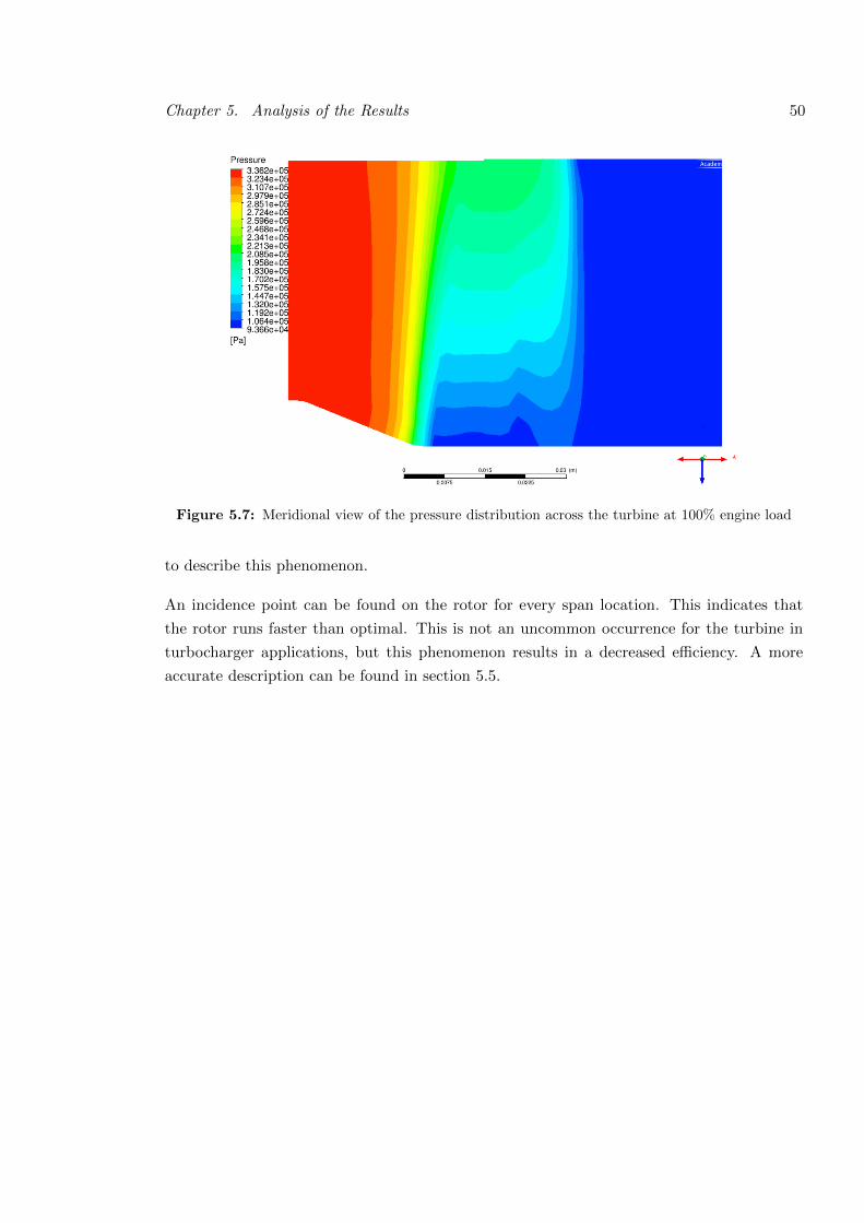
Chapter 5. Analysis of the Results 50
Figure 5.7: Meridional view of the pressure distribution across the turbine at 100% engine load
to describe this phenomenon.
An incidence point can be found on the rotor for every span location. This indicates that
the rotor runs faster than optimal. This is not an uncommon occurrence for the turbine in
turbocharger applications, but this phenomenon results in a decreased efficiency. A more
accurate description can be found in section 5.5.

Chapter 5. Analysis of the Results 51
Figure 5.8: Mach number distribution at 20% span at 100% engine load
Figure 5.9: Mach number distribution at 50% span at 100% engine load

Chapter 5. Analysis of the Results 52
Figure 5.10: Mach number distribution at 80% span at 100% engine load
5.3 Turbine Mass Flow Choking
In Figure 5.11, the h-s diagram for an axial turbine is shown. At high pressure ratios choking
may occur in either the stator or the rotor. From [6]:
In the stator applies:
h01 = h1 +1
2v2
1 (5.7)
v1 = c1 is reached for:
v21 = c2
1 = (γ − 1)h1, so h01 =γ + 1
2h1 (5.8)
The corresponding pressure ratio and mass flow rate are:
p1
p01=
(h1
h01
) nn−1
=
(2
γ + 1
) nn−1
(5.9)
mc = A1ρ01c01
(h1
h01
) 1n−1
+ 12
(5.10)
with n being the polytropic exponent and A1 the nozzle ring area (100cm2).
In the rotor, sonic state is achieved for:
w22 = (γ − 1)h2 (5.11)

Chapter 5. Analysis of the Results 53
Figure 5.11: h-s diagram for an axial turbine [6]
So,
h01 − u1v1u =γ + 1
2h2 −
1
2u2
2 (5.12)
andh2
h01=
2
γ + 1
(1−
u1v1u − 12u
22
h01
)(5.13)
Pressure ratio and mass flow rate with chocking are then:(p2
p01
)=
(h2
h01
) nn−1
=
(2
γ + 1
) nn−1
(1−
u1v1u − 12u
22
h01
) nn−1
(5.14)
mc = A2ρ01c01
(h2
h01
) 1n−1
+ 12
(5.15)
with A2 the rotor flow area (153cm2).
The choking mass flow rates for both stator and rotor can be calculated from the acquired
data from CFX calculations, with a polytropic exponent estimated by:
p2
p1=
(ρ2
ρ1
)n=⇒ n = 2.32 (5.16)
The polytropic exponent is greater than the specific heat ratio (γ) because of the inefficiencies
of the expansion and the loss of heat to the environment.

Chapter 5. Analysis of the Results 54
The mass flow rates for choking are 4.606kg/s in the stator and 6.209kg/s in the rotor. The
stator obviously determines choking. The mass flow rate with choking is then independent
of the rotational speed. In that case, the mass flow rate in function of pressure ratio can be
described with the graph displayed in Figure 5.12. With an exhaust mass flow rate of 4.47kg/s
at 3400kW the turbine is operating in conditions very near to choking. It is presumable that
due to the pulsating flow, instantaneous full choking may occur in the turbine.
Figure 5.12: Mass flow rate in function of pressure ratio for choking in the stator [6]
5.4 Stator Analysis
In this section, the flow field is analysed for the turbine stator at various operating points.
In order to understand the shape of the best fitting curve in Figure 5.2, which is mainly
determined by the flow in the stator, the flow field is analysed at four different points: One
point at low pressure ratio (πtot−st=1.665), before the maximum, one point just past the
maximum of the curve (πtot−st=2.824), and two points in choking conditions: at πtot−st=3.8
and at πtot−st=5.
The flow fields in the stator are numerically calculated with a different mesh then before. The
quality of the mesh presented in chapter 3 is good enough to determine the turbine properties
(as determined with the grid independence test), but in order to have good contour plots of
the transonic flow in the stator, a refinement of the mesh is needed in the regions were
supersonic flow and/or shocks are expected to occur. The mesh is constructed with the same
grid topology as the standard mesh, but with finer parameters and is refined at the necessary
locations. The maximum y+ value found in the meshes is 1.102E+00. It is unnecessary
to discuss this mesh in detail because the discussion would be similar to the discussion in
chapter 4, an overview of the mesh is provided in Appendix B.

Chapter 5. Analysis of the Results 55
A CFD simulation with a large mesh size needs long calculation times. In order to shorten
the calculation time and allow for mesh adaptation during the solution process, the analysis
is executed without a rotor grid. In order to get a good initial ‘guess’of the solution flow
field and especially the boundary conditions at the stator outlet, an initialising calculation
is executed with the standard stator mesh and with the rotor attached to the flow field.
The results from these initialising calculations are used as input for the actual calculations.
When all the input data is determined, the CFD simulation can start. The convergence
is checked during the iterations with monitors showing the root-mean-squared residuals of
flow properties. The simulations are performed in sub-steps. When a sub-step is converged,
the mesh size is adapted and refined at the locations with the greatest pressure, velocity,
and temperature gradients. The flow fields resulting from this method are more accurate
than the flow fields received from iterations with the standard mesh. However, it does not
result in significantly different property results (as shown by the grid independence test).
This supports anew the choice of a relatively coarse mesh for the standard calculations, since
iterations with this fine mesh could take up to 40 hours, for a stator-only calculation.
Pressure ratio 1.665
The first flow field analysed, is the flow field at a pressure ratio of 1.665. This pressure ratio is
chosen because this operating point was already used to validate the grid to experimental data
in Chapter 4. A total-to-static pressure ratio is very low, so no supersonic flow is expected.
Indeed, from Figure 5.13, it can be seen that the flow remains subsonic throughout the flow
field.
The general flow across the stator vanes is accelerating, and the highest velocities (and lowest
pressures) are found at the suction side of the blade. This increasing velocity results in a
wide boundary layer towards the trailing edge. Also visible on Figure 5.13 is the large wake
flow initiating from the trailing edge of the blade, disturbing the flow field in that region.
Pressure ratio 2.824
The second flow field is at a total-to-static pressure ratio of 2.824. Similar to the previous op-
erating point, the results gained from the experimental data validation were used to initialise
the flow field and the boundary conditions.
A pressure ratio of 2.824 is just greater than the pressure ratio at which maximum in the
best fitted efficiency curve is expected. Figure 5.14 shows the Mach number and pressure
plots of the flow field. Around this pressure ratio, the flow field alters from being entirely
subsonic, and at the suction side of the vane, sonic speed is reached in one point. With
increasing pressure ratios, this point grows into a supersonic zone, ending in a normal shock.
The supersonic zone is clearly influenced by the interaction with the trailing edge of the

Chapter 5. Analysis of the Results 56
neighbouring blade. After the normal shock, the boundary layer becomes wider. Note that
in the figure describing the Mach number, the plot limits are altered so that this supersonic
zone is better visible.
The normal shock ending the supersonic zone at the suction side, results in shock losses and
due to small radial differences in the shock intensities, strongly rotational flow. This all leads
to a decrease of the turbine efficiency.
Figure 5.13: Mach number and pressure plots in the stator at total-to-static pressure ratio 1.665
Figure 5.14: Mach number and pressure plots in the stator at total-to-static pressure ratio 2.824

Chapter 5. Analysis of the Results 57
Pressure ratio 3.8
At a total-to-static pressure ratio of 3.8, the flow reaches sonic speed at the throat section
between the suction side of the blade and the trailing edge of the neighbouring blade. The
supersonic zone has grown to cover the throat section. In the flow field, the large supersonic
zone is visible, with a strong, normal shock at the end. The wake flow of the neighbouring
blade is again very influential on the shape of this supersonic zone.
The normal shock hits the boundary layer of the suction side of the blade. The interaction
with the boundary layer creates a lambda shaped bifurcation. Figure 5.16 [33] shows this
interaction. Due to the impinging shock, the boundary layer becomes wider and the shock
deflects somewhat (the shock is normal to the flow). Because of the concave curvature of
the boundary layer before the shock, compression waves are generated, that converge in the
first leg of the lambda-shock. The convex curvature of the flow after the shock results in an
expansion, with a small supersonic zone after the shock wave.
Figure 5.15: Mach number and pressure plots in the stator at total-to-static pressure ratio 3.8
Figure 5.16: Shock-boundary layer interaction of a normal shock [33]

Chapter 5. Analysis of the Results 58
Pressure ratio 5
Figure 5.17 shows the flow field in the stator at a high total-to-static pressure ratio of 5 across
the turbine. The flow field at such a high pressure ratio is rather complex. The supersonic
zone as seen at lower pressure ratios, has reached the trailing edge of the blade, and is very
distorted.
Two oblique shocks depart from the trailing edge of the blade. One of those shocks hits
the suction side boundary layer of the blade. The interaction of this oblique shock with
the boundary layer can be explained with Figure 5.18 [33]. Because of the impinging oblique
shock, the boundary layer becomes wider. The shock reflects on the sonic line in the boundary
layer (represented by the dashed line in Figure 5.18).
At this pressure ratio, the flow field is not much different from the typical flow field found
in transonic rotor cascades with low degree of reaction. Figure 5.19 shows a sketch of such a
flow field. This is not a surprising result. The optimization of a stator cascade is not much
different from a rotor cascade for axial turbines, the main difference is the greater acceleration
found in stator cascades.
Figure 5.17: Mach number and pressure plots in the stator at total-to-static pressure ratio 5

Chapter 5. Analysis of the Results 59
Figure 5.18: Shock-boundary layer interaction of an oblique shock [33]
Figure 5.19: Sketch of the flow pattern in a transonic rotor cascade with low degree of reaction [6]
5.5 Rotor Analysis
The characteristic of the turbine is made up out of data points at different rotor speeds.
For every rotor speed there is a pressure ratio at which maximum efficiency is reached. In
Figure 5.20 the data points for different rotor speeds are shown. The data received from
KBB for this characteristic, does not contain data for pressure ratios above the optimum
for the different speed lines. This is because these operating points are hard to measure in
an experimental turbocharger test. The turbine does not operate at such a point during
operation. Nevertheless, it is interesting to study why the efficiency curves show a maximum
for every speed lines. The 24000 rpm speed line is analysed in this section. Figure 5.21 shows
the velocity vectors field at the leading edge of the rotor (50% span) at a total-to-static
pressure ratio of 1.665. At this pressure ratio, a low efficiency is reached (0.741 from KBB
data, 0.707 from CFX calculated data) for the speed line. The rotor is running at a higher

Chapter 5. Analysis of the Results 60
Figure 5.20: Rotor speed dependency of the efficiency
speed than optimal, resulting in an incidence on the suction side of the rotor blade near the
leading edge. The flow angle β1 is 22°, while the blade angle is 24°, so there is an incidence
of 2°. Due to this incidence, the flow separates at the pressure side of the rotor blade. The
flow shows rotations in this separated zone. A separated flow on the rotor surface results in
a lower efficiency.
Figure 5.22 shows the velocity vectors field at the leading edge of the rotor (50% span) at a
total-to-static pressure ratio of 1.9. This pressure ratio is near to the optimum for maximum
efficiency. At this point, there was no experimental data available, but a CFX calculation
resulted in an effective turbine efficiency of 0.806. As can be seen from the figure, the actual
relative flow angle β1 (24.5°) is close to the blade angle (24°), resulting in very low incidence
losses. The figure shows no separation of the flow at the pressure side of the rotor blade.
A pressure ratio of 2 is applied to the turbine with a rotor speed of 24000 rpm, in search of a
flow with no incidence on the rotor. The velocity field of this numerical simulation is shown
in Figure 5.23. The velocity vectors follow the shape of the blade. It is expected that this is
the point of maximum efficiency for a rotor speed of 24000, but the results show otherwise: a
turbine efficiency of 0.792 is found. This value is lower than the efficiency at a pressure ratio
of 1.9. A reason for this lowered efficiency is unknown.
Figure 5.24 shows the velocity vectors field at the leading edge of the rotor (50% span) at
a total-to-static pressure ratio of 2.5. This is far beyond the optimum pressure ratio for a
rotor speed of 24000 rpm. The relative angle of the flow is much larger than the blade angle,

Chapter 5. Analysis of the Results 61
resulting in an incidence point on the pressure side of the blade and a turbulent boundary
layer on the suction side. The turbine efficiency has dropped to 0.682 at this pressure ratio.

Chapter 5. Analysis of the Results 62
Figure 5.21: Velocity vectors plot at the leading edge of rotor at 50 % span, 24000 rpm, pressure
ratio 1.655
Figure 5.22: Velocity vectors plot at the leading edge of rotor at 50 % span, 24000 rpm, pressure
ratio 1.9

Chapter 5. Analysis of the Results 63
Figure 5.23: Velocity vectors plot at the leading edge of rotor at 50 % span, 24000 rpm, pressure
ratio 2
Figure 5.24: Velocity vectors plot at the leading edge of rotor at 50 % span, 24000 rpm, pressure
ratio 2.5

Chapter 6
Axial Turbine Geometry
Adjustment
6.1 Introduction
The turbine needs to be adjusted for higher mass flow rates. In the previous chapter it was
found that due to the turbine´s low degree of reaction, the stator is more prone to choking.
The mass flow rate at choking conditions in the stator is defined by the formula:
mc = A1ρ01c01
(h1
h01
) nn−1
+ 12
(6.1)
In order to adjust the turbine performance for larger mass flow rates, the most important
parameter to adjust is A1, the stator flow area or nozzle ring area. The goal of an increased
flow area is to reduce the stator outlet velocity v1, increasing the margin for choking. A few
possible solutions are proposed:
� Remove one or more stator vanes
� Rotate the stator vanes for smaller α1
� Reduce the thickness of the stator vanes
� Decrease the inner diameter of the turbine
� Increase the outer diameter of the turbine
Removing one or more stator vanes (with a rearrangement of the remaining stator blades)
would increase the stator flow area significantly. However, attention should be given to the
optimum solidity of the cascade (ratio of chord c to spacing s). A low solidity (and thus high
flow area) could possible result in insufficient guidance of the flow. A lower amount of stator
64

Chapter 6. Axial Turbine Geometry Adjustment 65
vanes would not be desirable for the production process as well. The stator rings constructed
by KBB always consist of 20 stator vanes. Removing one or more vanes and redistributing
the stator vanes over the circumference would significantly alter the production process.
Rotating the stator vanes to create a lower flow angle α1 lowers the outlet velocity of the
stator v1. The effects from a rotated stator blade are shown in Figure 6.1. A rather small
reduction of the stator outlet velocity v1 would require a large reduction of the rotor speed
u. This significantly changes the kinematic parameters of the cascade. The work coefficient
ψ = v1u−v2uu = ∆W
u2 , the flow coefficient ϕ = vau , and the degree of reaction R = −wmu
u , all
increase. Additionally, the outlet swirl in the contra-rotational sense (v2u < 0) increases.
The significantly decreased rotor speed is also not desirable for the radial compressor driven
by the turbine.
Figure 6.1: Effects of a lower flow angle α1 on the velocity triangles
The third proposed solution is to change the thickness of the blade. This, however, would
severely deteriorate the structural integrity of the stator vanes. Due to the pulsating flow
in the exhaust manifold of the engine, turbocharger turbine stator vanes and rotor blades
typically are thicker than in gas turbines for other applications.
The fourth and fifth proposed solution for reducing the stator outlet velocity v1 aim for
the same result. However, the idea of decreasing the inner diameter of the turbine blades
is quickly scraped. This would require the turbocharger shaft to have a smaller diameter,
reducing the structural integrity of this shaft. An increased outer diameter then seems a
better solution at first sight.
An increased outer diameter of the turbine increases the flow area through the turbine. This
results in a lower axial flow velocity. The effect from this lowered axial velocity is shown in
Figure 6.2. Similarly to the effects when decreasing the flow angle α1, the decreased axial
velocity results in a lower rotor speed, but the decrease of rotor speed is less. The kinematic
parameters are expected to remain the same.

Chapter 6. Axial Turbine Geometry Adjustment 66
Figure 6.2: Effects of a lower flow angle α1 on the velocity triangles
6.2 Adjustment Method
Together with ABC, the decision is made to check the results of the increased diameter on
the parameters of the turbine. The increased diameter is chosen by a simple rule of three,
based on the power output of the engine and the flow area at the interface between stator
and rotor:
AnewAT266
=4000kW
3400kW(6.2)
Where:
AT266 = πD2 − d2
4= π
0.2662 − 0.1602
4= 0.0355m2 (6.3)
Anew = πD2new − 0.1602
4(6.4)
From these calculations, an outer diameter of 276 mm is chosen. This method of choosing
the outer diameter is arbitrary. In order to chose an ideal outside diameter of the turbine,
more careful considerations should be made. The goal of the following sections is to study if
an increased outside diameter is beneficial for the operation of both turbocharger and diesel
engine, knowingly that a non-optimal diameter is chosen.
6.2.1 Adjusting the Stator
As mentioned in section 3.2, the stator vanes are prismatic. This simplifies the extension of
vanes. The blade profiles for the stator are provided at the hub and at the shroud of the T266
turbine. As a simplification, the blade profile at 100% span for the T266 turbine is used at
100% span for the ‘T276’ turbine.

Chapter 6. Axial Turbine Geometry Adjustment 67
6.2.2 Adjusting the Rotor
The torsioned rotor blades are much more difficult to extend to a blade height of 58 mm.
The strategy used for extending the stator vanes is not usable for the extension of the rotor
blades, a geometrical redistribution of the profiles to a blade height of 58 mm is not advisable.
To construct a profile at this blade height, an extrapolation of the provided blade profiles is
executed.
The first step was to extrapolate the location of the leading edge for the blade profiles to
the new blade height. Figure 6.3 shows this extrapolation. With the location of the leading
edge set, the profile is constructed in the local coordinate frame. This is shown in Figure
6.4. With the formulas (3.1) and (3.2) the profile coordinates are transformed to the global
reference frame (with θ, a and b extrapolated analogous to the extrapolation of xp and yp).
The resulting blade profile is shown in Figure 6.5. Similarly to before, circular leading and
trailing edges are obtained by adding points as part of a circle.
Figure 6.3: Location of the leading edge at blade height Z

Chapter 6. Axial Turbine Geometry Adjustment 68
Figure 6.4: Blade profiles in local coordinate frame
Figure 6.5: Blade profiles in global reference frame

Chapter 7
Results
7.1 Introduction
With the geometry of the T276 turbine constructed in the previous chapter, The grid is
constructed and the preprocessing is executed in a similar method as in chapter 3. It is
unnecessary to discuss the grid for the new turbine, because the grid discussion was already
done in chapter 3.
It is intended to construct the characteristic of the turbine and get an estimate of its perfor-
mance on the ABC 16VDZC engine. Without a GT power analysis of the engine with the
turbine data, it is not possible to get results for the performance on the engine, but with
the acquired turbine characteristics, an estimation can made of the operating range of the
turbine on the engine.
7.2 SAE Data map
As a first step a data map for the T276 turbine is constructed. The input data used for
the construction of such a map was derived from the data used for the T266 turbine. The
SAE data map of the T266 contains speed lines at constant rotational speeds. To measure
the performance of the turbine at constant speed and at different pressure ratios on an
experimental test bed, the total inlet temperature needs to be adjusted for every operating
point. This results in different reduced speed values (formula ()4.2)) on a speed line.
By calculating the performance data with numerical iterations, operating points can be
checked for constant reduced speed values. This improves the applicability of the data map
for 1D simulation software like GT-power. The reduced speeds are shown in Table 7.1. The
Inlet temperatures are based on the inlet temperatures provided by KBB for the first point
at every speed line for the T266 turbine. Three SAE data maps are found in Appendix A: the
69

Chapter 7. Results 70
data provided by KBB for the T266 turbine and the data obtained by numerical iterations
for both the T266 en the T276 turbine.
n (rpm) T00 (K) nreduced(rpm/√K)
24000 908 797
27000 801 953
30000 783 1071
33000 824 1150
35000 860 1195
37000 892 1239
Table 7.1: The Reduced speed lines for the T276 turbine
The different speed lines are constructed with the pressure ratios and rotor speed as provided
for the T266 turbine, but the total inlet temperature is kept constant over a speed line. The
resulting efficiency characteristic is plotted in Figure 7.1. The efficiency data provided by
KBB and the efficiency data obtained from the numerical iterations for the T266 turbine are
plotted as a comparison. From the graph, it can be seen that the best fitted efficiency curve
has shifted to higher pressure ratios. At low pressure ratios, the efficiency of the adjusted
turbine is lower than the efficiency of the T266, this is to be expected as the flow area is
larger and thus the axial velocity lower. At high pressure ratios the efficiency of the turbine
is higher. At these pressure ratios the flow shows a supersonic zone on the suction side of the
stator vanes for the smaller turbine, which generate shock losses (see Chapter 5). Because
of the higher flow area, the axial velocity is lower, and the critical point at which supersonic
flow occurs is moved to higher pressure ratios.

Chapter 7. Results 71
Figure 7.1: Comparison of turbine efficiencies
In order to create a good data map for 1D simulation software, it is useful to complement
the speed lines with values at the decreasing part of the curve. These values were added for
the speed lines of the T276 turbine by numerical simulations at higher pressure ratios. For
the speed lines at 24000 rpm and 27000 rpm this is not necessary, because the last value is
already on the decreasing part of the curve. Table 7.2 shows the input data for the other
speed lines. The results from these simulations are shown in Figure 7.2. The best fitted
curves for every speed line are plotted in the graph as well.
n (rpm) πtot−st T00 (K) p00(kPa) p2 (kPa)
30000 2.7 783.64 273.578 101.325
33000 3.1 824.54 314.108 101.325
35000 3.3 860.04 334.373 101.325
37000 3.5 892.24 354.638 101.325
Table 7.2: Input data used for completing the speed lines in the data map
Figure 7.3 shows the mass flow rates through the T276 turbine at different pressure ratios, in
comparison to the mass flow rates through the T266 turbine. In this curve we can see that at
low pressure ratios, there is little difference in mass flow rates between the two turbines. At
higher pressure ratios, the difference increases. The T266 turbine nearly reaches the pressure
ratio for choking and the mass flow rate curve converges to the choking mass flow rate, while
the T276 turbine is still far enough away from choking and the convergence of the mass flow
rate curve is not yet observable.

Chapter 7. Results 72
Figure 7.2: Complete efficiency curve of the T276 turbine constructed with numerical simulations
Figure 7.3: Mass flow rate

Chapter 7. Results 73
7.3 Performance Analysis
In this section, the performance of the turbine is analysed, based on the results from the
numerical iterations presented in Section 7.2. First of all, we can see that the new turbine is
a definite improvement over the T266 turbine, despite of the particularly simple adjustment
made ot the turbine. The turbine has a higher efficiency and a higher mass flow rate at a
total-to-static pressure ratio of 3.31, which was the pressure ratio of the smaller turbine at
100% engine load.
The operating point of the T276 turbine on the 16VDZC will be different, and cannot be
determined accurately without 1D simulation software. However, with a few considerations an
estimation of the turbine operating point can be made. For the same mass flow rate through
the turbines, the exhaust manifold pressure and thus the turbine inlet pressure for the turbine
with greater flow area will be lower. This results in a lower pressure ratio. In order to make
a comparison between the adjusted turbine and the T266 turbine, two operating points are
interesting:
� an operating point with mass flow rate close to the mass flow rate obtained in the
CFX simulations for engine power output 3400kW: m = 4.95 kg/s with rotor speed
35419 rpm and pressure ratio 3.31. The operating point from the turbine characteristic
(Section 7.2) with similar values is: m = 5.04 kg/s with rotor speed 33032 rpm and
pressure ratio 2.96.
� an operating point with the same pressure ratio and rotor speed as the T266 turbine
with an engine power output of 3400kW: Rotor speed 35419 rpm and pressure ratio
3.31. The mass flow rate through the T276 is higher for this pressure ratio. This
operating point for the T276 turbine is expected to accommodate to a higher engine
power output.
The real operating point of the turbine at 100% engine load will be between these two points.
It is not possible with 1D CFD simulation software to get a better estimate, but from the
turbine characteristics (Figure 7.1 and Figure 7.3) it can be derived that any operating point
in this range will result in an improved performance on the engine.

Chapter 8
Conclusions and Recommendations
In this final chapter, some conclusions based on the work exerted for this master’s dissertation
are given, with some recommendations for further research on the matching of turbochargers
on medium speed diesel engines.
The matching of a turbocharger on a engine is a very difficult task. In this work it is shown
that with the help of CFX and TurboGrid, reasonably accurate turbine characteristics can
be generated for the exhaust gas turbine, in a reasonable timespan. These characteristics
allow for a faster selection of a correct turbocharger. If a more profound analysis of the flow,
it is possible to create very fine grids and very accurate results can be achieved.
The T266 was working in near choking conditions, resulting in a low efficiency at full load,
which is not desirable for a diesel engine mainly used in combination with a generator to
produce electrical power. In order to find a possible solution to the turbine choking condi-
tions, the stator flow area was increased with a simplistic adjustment to the geometry. This
adjustment results in a greater mass flow rate and higher efficiency at the same pressure
ratios provided by the engine test. Due to the greater stator flow area, the pressure in the
exhaust manifold is expected to drop. This is beneficial for the engine power, and will result
in a lower turbine pressure ratio. This is in line with the considerations made in the first
chapter of this dissertation. By comparing the 8DZC and 16VDZC engines, it was found that
the total pressure in the exhaust manifold for the 16VDZC was much higher.
The results gathered in Chapter 7 of this thesis show that the increase of the outside diameter
is a possible solution for the turbine. However, with the tools at hand, it was impossible to
construct a good design for the turbine blades, and so a simplistic extrapolation was done
on the profiles of the blade. An analysis with better designed blades should be executed in
order to get better results.
The effect of the adjusted turbine on the engine can not be analysed with 3D CFD simulations
74

Chapter 8. Conclusions and Recommendations 75
alone. For this, an analysis with 1D simulation software like GT power has to be executed.
Especially the operation of the compressor driven by the turbine should be taken into con-
sideration. The compressor map of the C184B2 20P8-15.0 compressor has been provided in
Appendix C. The flow area in the centrifugal compressor will have to be increased as well, if
the mass flow rate increases too much.
In Chapter 6, the choice of increasing the diameter was documented and it was opted to be
the right choice. However, the efficiency of the turbine is much lower at lower pressure ratios
and thus at lower engine loads. As stated before, this is not important for power generation,
but in marine or locomotive applications this result is not wanted. In that case a rotation of
the stator vanes is a better choice, if it is implemented with a system allowing for variable
nozzle area by rotating the stator vanes. A small nozzle area should then be used at lower
loads, and the maximum area at full load.

Appendix A
SAE data maps
SAE data map T266/100 as provided by KBB
nreduced mreduced πtot−st ηeT T00
(rpm/√K) ((kg/s)
√K/kPa) (K)
797.0765 0.3696 1.655 0.741 908.04
847.4805 0.3747 1.738 0.7651 803.44
885.9373 0.3794 1.809 0.7771 730.74
919.5953 0.3807 1.868 0.7849 678.34
952.6929 0.3845 2.007 0.7755 801.64
995.7891 0.3885 2.117 0.7907 736.04
1027.435 0.3881 2.184 0.8007 691.14
1071.918 0.3894 2.421 0.7963 783.64
1081.816 0.3896 2.449 0.7967 770.34
1105.705 0.3916 2.523 0.8024 735.94
1129.505 0.3902 2.583 0.8119 706.24
1150.201 0.3922 2.824 0.787 824.54
1182.203 0.3932 2.956 0.7926 780.74
1208.578 0.3914 3.027 0.8027 747.94
1195.16 0.394 3.112 0.7769 860.04
1222.554 0.3956 3.225 0.7805 819.54
1243.86 0.3928 3.256 0.7891 794.24
1239.984 0.3924 3.39 0.7723 892.24
1254.551 0.3936 3.431 0.774 870.04
1267.441 0.3947 3.449 0.7705 852.94
Table A.1: SAE data map T266/100 turbine provided by KBB
76

Appendix A. SAE data maps 77
SAE data map T266/100 obtained with CFX numerical itera-
tions
nreduced mreduced πtot−st ηeT T00
(rpm/√K) ((kg/s)
√K/kPa) (K)
797.0765 0.418765 1.655 0.702918 908.04
847.4805 0.423674 1.738 0.736737 803.44
885.9373 0.426655 1.809 0.75804 730.74
919.5953 0.428308 1.868 0.736739 678.34
952.6929 0.431316 2.007 0.752217 801.64
995.7891 0.431697 2.117 0.783801 736.04
1027.435 0.431304 2.184 0.761662 691.14
1071.918 0.429285 2.421 0.769933 783.64
1081.816 0.428814 2.449 0.776008 770.34
1105.705 0.42753 2.523 0.789891 735.94
1129.505 0.426338 2.583 0.799695 706.24
1150.201 0.421762 2.824 0.786884 824.54
1182.203 0.418929 2.956 0.803321 780.74
1208.578 0.417323 3.027 0.810905 747.94
1195.16 0.415677 3.112 0.790977 860.04
1222.554 0.413255 3.225 0.802126 819.54
1243.86 0.41251 3.256 0.804922 794.24
1239.984 0.409868 3.39 0.791543 892.24
1254.551 0.411915 3.431 0.795027 870.04
1267.441 0.408585 3.449 0.796477 852.94
Table A.2: SAE data map T266/100 obtained with CFX numerical iterations

Appendix A. SAE data maps 78
SAE data map T276/100 obtained with CFX numerical itera-
tions
nreduced mreduced πtot−st ηeT T00
(rpm/√K) ((kg/s)
√K/kPa) (K)
797.0765 0.480599 1.655 0.702918 908.04
797.1755 0.488622 1.738 0.736737 908.04
794.7526 0.493595 1.809 0.75804 908.04
794.8185 0.4966 1.868 0.736739 908.04
952.6929 0.495751 2.007 0.752217 801.64
954.1758 0.497567 2.117 0.783801 801.64
953.9988 0.497912 2.184 0.761662 801.64
1071.918 0.493967 2.421 0.769933 783.64
1072.596 0.493689 2.449 0.776008 783.64
1071.524 0.492689 2.523 0.789891 783.64
1072.274 0.491695 2.583 0.799695 783.64
1071.675 0.491023 2.7 0.778049 783.64
1150.201 0.485918 2.824 0.786884 824.54
1150.375 0.48299 2.956 0.803321 824.54
1151.071 0.481389 3.027 0.810905 824.54
1149.233 0.480176 3.1 0.796861 824.54
1195.16 0.479052 3.112 0.790977 860.04
1193.421 0.476482 3.225 0.802126 860.04
1195.33 0.475776 3.256 0.804922 860.04
1193.462 0.474981 3.3 0.794091 860.04
1239.984 0.472472 3.39 0.791543 892.24
1238.845 0.47156 3.431 0.795027 892.24
1239.213 0.471159 3.449 0.796477 892.24
1238.685 0.47067 3.5 0.791872 892.24
Table A.3: SAE data map T276/100 obtained with CFX numerical iterations

Appendix B
Stator Mesh for flow analysis
79

Appendix B. Stator Mesh for flow analysis 80
Figure B.1: The fine mesh used for the stator analysis (Section 5.4)
Figure B.2: detail of the fine mesh near the trailing edge of the stator vane

Appendix B. Stator Mesh for flow analysis 81
Figure B.3: y+ values

Appendix C
Compressor Data map
82

COMPRESSOR MAP M40
M400802e01
.
ISE
NT
RO
PIC
CO
MP
RE
SS
OR
WO
RK
(to
tal-t
otal
) h
isC
_298
[kJ
/kg]
CO
MP
RE
SS
OR
PR
ES
SU
RE
RA
TIO
(to
tal-t
otal
) π
C
1.0
1.5
2.0
2.5
3.0
3.5
4.0
4.5
5.0
0.5 1.0 1.5 2.0 2.5 3.0 3.5 4.0
0.81
0.80
0.80
0.79
0.73
0.75
0.78
AIR FLOW RATE V298 [m3/s]
bCbC298 T
298KVV && =
bC298 T
298Knn =
n298=24000 min-1
27000
30000
33000
35000
37000
C184B2 20P8-15.0nmax=37000 min-1
(with Air-Intake Bend)
0
10
20
30
40
50
60
70
80
90
100
110
120
130
140
150
160
170

Bibliography
[1] IMO, “www.imo.org,” Feb 2014.
[2] K. Matsumoto, “Development of high-pressure ratio and high-efficiency type turbo-
charger,” CIMAC congress Shanghai, 2013.
[3] U. Schlemmer-Kelling, “The environment friendly medium speed engine,” CIMAC
congress Vienna, 2007.
[4] P. Neuenschwander, “New turbochargers for more powerful engines running under
stricter emission regimes,” CIMAC congress Bergen, 2010.
[5] M. Oana, O. Kawamoto, H. Ohtani, and Y. Yamamoto, “Approach to high-performance
compressor design. Japan: Journal of Propulsion and Power,” Journal of Propulsion and
Power, vol. 20, pp. 164–170, January-February 2004.
[6] E. Dick, “Gasturbines,” 2013.
[7] K. Matsumoto, “Development of high-pressure ratio and high-efficiency type turbo-
charger,” CIMAC congress Shanghai, 2013.
[8] H. Tamaki, “Effect of recirculation device with counter swirl vane on performance of
high pressure ratio centrifugal compressor,” Journal Of Turbomachinery-Transactions
of the ASME, vol. 134, SEP 2012.
[9] R. Hunziker, P. Jacoby, and A. Meier, “A new series of small turbochargers for high flow
rates and high pressure ratios,” CIMAC congress Hamburg, 2001.
[10] P. Roach, “The role of CFD in turbocharger performance improvement,” CIMAC
congress Vienna, 2007.
[11] J. Klima, V. Hort, and M. Haidn, “TCX - the new high pressure turbocharger for two
stage turbocharging,” CIMAC congress Shanghai, 2013.
[12] S. Kim, J. Park, K. Ahn, and J. Baek, “Improvement of the performance of a centrifugal
compressor by modifying the volute inlet,” Journal Of Turbomachinery-Transactions of
the ASME, vol. 132, SEP 2010.
84

Bibliography 85
[13] C. Lutzen, A. Moller, and C. Christensen, “Turbocharger failures, a law of nature or
neglect,” CIMAC congress Hamburg, 2001.
[14] A. Rippl, “Engine builder’s and customer’s demands made on an exhaust gas turbo-
charger and their consequent realisation in a new developed turbocharger generation,”
CIMAC congress Hamburg, 2001.
[15] A. Bornhorn, S. Mayr, and T. Winter, “3D-Fluid-Structure interaction for an axial turbo-
charger turbine blade to improve the vibrational safeguard process,” CIMAC congress
Bergen, 2010.
[16] J. Klima, M. Vacek, and O. Tomek, “High performance small turbochargers,” CIMAC
congress Bergen, 2010.
[17] K. Buchman and R. Drozdowski, “ST27: A new generation of radial turbine turbocharg-
ers for highest pressure ratios,” CIMAC congress Bergen, 2010.
[18] P. Jacobi, H. Xu, and W. David, “VTG turbocharging - a valuable concept for traction
application,” CIMAC congress Shanghai, 2013.
[19] H. Tamaki, M. Unno, A. Iwakami, and S. Ishii, “Study on flow fields in variable area
nozzles for radial turbine,” CIMAC congress Vienna, 2007.
[20] D. Zigan, W. Heintze, and U. Kramer, “VRT - A new turbocharging system for high
torque,” 1998.
[21] T. Takanori, K. Masanori, and S. Keiichi, “Development of new turbocharger technology
for energy efficient and low emission diesel power plant,” CIMAC congress Bergen, 2010.
[22] T. Raikio, B. Hallback, and A. Hjort, “Development of new turbocharger technology for
energy efficient and low emission diesel power plant,” CIMAC congress Bergen, 2010.
[23] J. Zhang, “Study on axial-radial turbocharger with pressure ratio 4.5,” 2007.
[24] T. Behr, M. Kahi, A. Reichi, and M. Hubacher, “Second generation of two-stage tur-
bocharging Power2 systems for medium speed gas and diesel engines,” CIMAC congress
Vienna, 2007.
[25] S. Risse and K. Buchman, “New turbochargers for modern large engines with low emis-
sions and high performance,” CIMAC congress Shanghai, 2013.
[26] D. Six and T. Van Herzele, “Development of emission reduction tehniques for medium
speed diesel engines with special focus on EGR,” master thesis, Ghent University, 2011.
[27] Y. Ono, “Solutions for better engine performance at low load by Mitsubishi turbocharg-
ers,” CIMAC congress Shanghai, 2013.

Bibliography 86
[28] L. Jie, Y. Yuting, and Z. Jizhong, “Numerical simulation investigation on centrifugal
compressor performance of turbocharger,” Journal of Mechanical Science and Technology
27, 2012.
[29] Y. Jun and Y. Yufeng, “CFD prediction and experimental measurement of blade water
coverage in a diesel turbocharger,” Modelling and Simulation in Engineering, vol. 2012.
[30] H. Tabatabaei, M. Boroomand, and R. M. Taeibi, “An investigation on turbocharger tur-
bine performance parameters under inlet pulsating flow,” Journal of Fluids Engineering,
vol. 134, 2012.
[31] L. Vervaeke and D. Vervaele, “Optimisation of a turbocharger,” master thesis, Ghent
University, 2003.
[32] J. Hauser and Y. Xia, Modern Introduction to Grid Generation. EPF Lausanne, 1996.
[33] J. Vierendeels, “Stromingsmechanica,” 2012.

List of Figures
1.1 IMO NOx emission limitations [1] . . . . . . . . . . . . . . . . . . . . . . . . 2
1.2 Pressure ratio and turbocharger efficiency required for current and future en-
gines [4] . . . . . . . . . . . . . . . . . . . . . . . . . . . . . . . . . . . . . . . 5
1.3 Mach number contours of the LE at midspan height for a radial transonic
compressor with pressure ratio 7.5 [5] . . . . . . . . . . . . . . . . . . . . . . 5
1.4 recirculation device on a radial turbocharger compressor [7] . . . . . . . . . . 6
1.5 A compressor map showing the influence (red) of a compressor case treatment
on the surge limit [8] . . . . . . . . . . . . . . . . . . . . . . . . . . . . . . . . 7
1.6 pressure distribution at radial compressor shroud [9] . . . . . . . . . . . . . . 7
1.7 Streamlines at a vaned diffuser showing the complex secondary flow [10] . . . 9
1.8 A circular leading edge (blue) and an elliptical leading edge (red) [10] . . . . 9
1.9 A polished (left), vs a milled (right) compressor diffuser [11] . . . . . . . . . . 9
1.10 (a) Standard turbine outlet collector design with flow features; (b) improved
turbine outlet collector design [10] . . . . . . . . . . . . . . . . . . . . . . . . 11
1.11 Variable turbine geometry for axial turbines[18] . . . . . . . . . . . . . . . . . 11
1.12 Variable geometry for radial turbines, principle [19] . . . . . . . . . . . . . . . 12
1.13 VRT with a sliding mechanism allowing for two different nozzle rings to be
used [20] . . . . . . . . . . . . . . . . . . . . . . . . . . . . . . . . . . . . . . . 13
1.14 A hybrid turbocharger by MHI [21] . . . . . . . . . . . . . . . . . . . . . . . . 15
1.15 Generator and motor function on a hybrid turbocharger [21] . . . . . . . . . . 15
1.16 examples of integrated turbocharger designs [22] . . . . . . . . . . . . . . . . 16
1.17 Cutaway view of an axial-radial turbocharger [23] . . . . . . . . . . . . . . . . 17
1.18 Optimal design point for intermediate pressure in two stage turbocharging [24] 18
2.1 Simulated characteristic curves of a turbocharger radial turbine under steady
and unsteady flow [30] . . . . . . . . . . . . . . . . . . . . . . . . . . . . . . . 23
3.1 Ansys CFD Environment . . . . . . . . . . . . . . . . . . . . . . . . . . . . . 25
3.2 The turbine geometry, the stator vanes [blue] and rotor blades [red] . . . . . . 26
3.3 Coordinate transformation scheme [31] . . . . . . . . . . . . . . . . . . . . . . 27
87

List of Figures 88
3.4 Matlab plot of the stator blade profiles . . . . . . . . . . . . . . . . . . . . . . 27
3.5 Matlab plot of the rotor blade profiles . . . . . . . . . . . . . . . . . . . . . . 28
3.6 The traditional grid topologies, with from left to right: H-grid, J-grid, C-grid,
L-grid . . . . . . . . . . . . . . . . . . . . . . . . . . . . . . . . . . . . . . . . 29
3.7 The topology used for the stator mesh . . . . . . . . . . . . . . . . . . . . . . 30
3.8 The computational grid used for the stator . . . . . . . . . . . . . . . . . . . 32
3.9 The topology used for the rotor mesh . . . . . . . . . . . . . . . . . . . . . . 33
3.10 The computational grid used for the rotor . . . . . . . . . . . . . . . . . . . . 34
4.1 Grid independence test . . . . . . . . . . . . . . . . . . . . . . . . . . . . . . . 38
4.2 y+ Values on the stator blade (left) and rotor blade (right) at 50 % span . . . 39
4.3 The turbine characteristics as provided by KBB . . . . . . . . . . . . . . . . . 40
4.4 Comparison of CFX calculated efficiencies to experimental values . . . . . . . 42
4.5 Comparison of CFX calculated mass flow rates to experimental values . . . . 42
5.1 CFX calculated turbine efficiencies and pressure ratios for engine data . . . . 45
5.2 Mass flow rate comparison between engine test and cfx data . . . . . . . . . . 45
5.3 Mass flow rate comparison between engine test and cfx data . . . . . . . . . . 46
5.4 velocity triangles at hub, midspan and shroud . . . . . . . . . . . . . . . . . . 47
5.5 Blade loading charts for stator (left) and rotor (right) . . . . . . . . . . . . . 48
5.6 Pressure distribution at 50% span . . . . . . . . . . . . . . . . . . . . . . . . 49
5.7 Meridional view of the pressure distribution across the turbine at 100% engine
load . . . . . . . . . . . . . . . . . . . . . . . . . . . . . . . . . . . . . . . . . 50
5.8 Mach number distribution at 20% span at 100% engine load . . . . . . . . . . 51
5.9 Mach number distribution at 50% span at 100% engine load . . . . . . . . . . 51
5.10 Mach number distribution at 80% span at 100% engine load . . . . . . . . . . 52
5.11 h-s diagram for an axial turbine [6] . . . . . . . . . . . . . . . . . . . . . . . . 53
5.12 Mass flow rate in function of pressure ratio for choking in the stator [6] . . . 54
5.13 Mach number and pressure plots in the stator at total-to-static pressure ratio
1.665 . . . . . . . . . . . . . . . . . . . . . . . . . . . . . . . . . . . . . . . . . 56
5.14 Mach number and pressure plots in the stator at total-to-static pressure ratio
2.824 . . . . . . . . . . . . . . . . . . . . . . . . . . . . . . . . . . . . . . . . . 56
5.15 Mach number and pressure plots in the stator at total-to-static pressure ratio
3.8 . . . . . . . . . . . . . . . . . . . . . . . . . . . . . . . . . . . . . . . . . . 57
5.16 Shock-boundary layer interaction of a normal shock [33] . . . . . . . . . . . . 57
5.17 Mach number and pressure plots in the stator at total-to-static pressure ratio 5 58
5.18 Shock-boundary layer interaction of an oblique shock [33] . . . . . . . . . . . 59
5.19 Sketch of the flow pattern in a transonic rotor cascade with low degree of
reaction [6] . . . . . . . . . . . . . . . . . . . . . . . . . . . . . . . . . . . . . 59
List of Figures 89
5.20 Rotor speed dependency of the efficiency . . . . . . . . . . . . . . . . . . . . . 60
5.21 Velocity vectors plot at the leading edge of rotor at 50 % span, 24000 rpm,
pressure ratio 1.655 . . . . . . . . . . . . . . . . . . . . . . . . . . . . . . . . . 62
5.22 Velocity vectors plot at the leading edge of rotor at 50 % span, 24000 rpm,
pressure ratio 1.9 . . . . . . . . . . . . . . . . . . . . . . . . . . . . . . . . . . 62
5.23 Velocity vectors plot at the leading edge of rotor at 50 % span, 24000 rpm,
pressure ratio 2 . . . . . . . . . . . . . . . . . . . . . . . . . . . . . . . . . . . 63
5.24 Velocity vectors plot at the leading edge of rotor at 50 % span, 24000 rpm,
pressure ratio 2.5 . . . . . . . . . . . . . . . . . . . . . . . . . . . . . . . . . . 63
6.1 Effects of a lower flow angle α1 on the velocity triangles . . . . . . . . . . . . 65
6.2 Effects of a lower flow angle α1 on the velocity triangles . . . . . . . . . . . . 66
6.3 Location of the leading edge at blade height Z . . . . . . . . . . . . . . . . . . 67
6.4 Blade profiles in local coordinate frame . . . . . . . . . . . . . . . . . . . . . . 68
6.5 Blade profiles in global reference frame . . . . . . . . . . . . . . . . . . . . . . 68
7.1 Comparison of turbine efficiencies . . . . . . . . . . . . . . . . . . . . . . . . . 71
7.2 Complete efficiency curve of the T276 turbine constructed with numerical sim-
ulations . . . . . . . . . . . . . . . . . . . . . . . . . . . . . . . . . . . . . . . 72
7.3 Mass flow rate . . . . . . . . . . . . . . . . . . . . . . . . . . . . . . . . . . . 72
B.1 The fine mesh used for the stator analysis (Section 5.4) . . . . . . . . . . . . 80
B.2 detail of the fine mesh near the trailing edge of the stator vane . . . . . . . . 80
B.3 y+ values . . . . . . . . . . . . . . . . . . . . . . . . . . . . . . . . . . . . . . 81

List of Tables
1.1 Comparison between different engines . . . . . . . . . . . . . . . . . . . . . . 3
3.1 Mesh Analysis . . . . . . . . . . . . . . . . . . . . . . . . . . . . . . . . . . . 31
3.2 Mesh Analysis . . . . . . . . . . . . . . . . . . . . . . . . . . . . . . . . . . . 33
4.1 Grid independence test . . . . . . . . . . . . . . . . . . . . . . . . . . . . . . . 38
5.1 engine input data . . . . . . . . . . . . . . . . . . . . . . . . . . . . . . . . . . 43
5.2 Rotor Flow angles . . . . . . . . . . . . . . . . . . . . . . . . . . . . . . . . . 47
5.3 Turbine Torque and power . . . . . . . . . . . . . . . . . . . . . . . . . . . . . 48
7.1 The Reduced speed lines for the T276 turbine . . . . . . . . . . . . . . . . . 70
7.2 Input data used for completing the speed lines in the data map . . . . . . . 71
A.1 SAE data map T266/100 turbine provided by KBB . . . . . . . . . . . . . . . 76
A.2 SAE data map T266/100 obtained with CFX numerical iterations . . . . . . 77
A.3 SAE data map T276/100 obtained with CFX numerical iterations . . . . . . 78
90

