development of a dynamical model for retina-based …tobi/wiki/lib/exe/fetch.php?media=ritz... ·...
TRANSCRIPT
Robin Ritz
Development of a DynamicalModel for Retina-based
Control of an RC MonsterTruck
Bachelor Project
Automatic Control LaboratorySwiss Federal Institute of Technology (ETH) Zurich
Advisors
Thomas BesselmannTobi Delbruck
Prof. Manfred Morari
September 11, 2008

Abstract
At the Institute of Neurinformatics (INI), a shared institute of the Uni-versity of Zurich (UZH) and the Swiss Federal Institute of TechnologyZurich (ETHZ), a dynamic vision sensor for fast visual processing hasbeen developed. The dynamic vision sensor uses a silicon retina to de-tect contrast changes in a scene. An ongoing project is to develop acontroller based on a silicon retina for a small robotic monster truck.The goal of the project is to drive at high speed along a drawn route. Inthis semester project, a dynamical model of the RC monster truck is de-rived and a simulation environment to test retina-based control strategiesis developed. The simulation is based on Blender, a powerful open-sourcemodeling environment. Further, first control strategies for event-basedlateral control are implemented and tested in the simulation, as well ason the real vehicle. At the end of this semester project, the truck is ableto follow a chalk drawn line at a little more than walking pace.
iii

Contents
Abstract iii
1 Introduction 1
2 Description of the RC Monster Truck 3
3 Modeling the RC Monster Truck 53.1 Assumptions . . . . . . . . . . . . . . . . . . . . . . . . . 53.2 Nonlinear Model . . . . . . . . . . . . . . . . . . . . . . 63.3 Reduced Model for Controller Design . . . . . . . . . . . 203.4 Parameter Identification . . . . . . . . . . . . . . . . . . 26
4 Simulation in Blender 284.1 Simulation Concept . . . . . . . . . . . . . . . . . . . . . 284.2 Implementation . . . . . . . . . . . . . . . . . . . . . . . 294.3 Simulation Results . . . . . . . . . . . . . . . . . . . . . 33
5 Controller Design 355.1 PID Control Scheme . . . . . . . . . . . . . . . . . . . . 355.2 LQR Control Scheme . . . . . . . . . . . . . . . . . . . . 375.3 Experimental Results . . . . . . . . . . . . . . . . . . . . 38
6 Conclusion 39
Acknowledgement 40
List of Figures 41
Attachments 42
Bibliography 43
v
1
1 Introduction
Cars with an automatic steering system are a current area of research.Modern cars already provide active assistance concerning steering anddrive power control and prototypes have been developed, which are ableto drive completely autonomous. Indeed, autonomous vehicles open afield of challenges which not all have been solved completely until today.One of these challenges, which are still a current area of research, is thevisual processing. An autonomous vehicle which can be used on commonroads must have visual sensors. Otherwise, the vehicle will not be ableto track the road. Since common cameras capture pictures on a constanthigh frame rate, they cause high requirements on the memory resources.In addition, the pictures have to be processed in real time to detect theroad and potentially to identify obstacles, what requires high processorresources. Hence, the cost for a system with good visual processing arehigh, since hardware resources are expensive. A further problem mightbe that the performance of the processors is limited, even if the cost haveno importance.
A new approach to avoid these problems are event-based visual sen-sors. The key idea of an event-based sensor is that only changes in themeasurement area are submitted. Thus, in the case of a visual sensor, ifa pixel of the picture does not change, then no information is generatedfor this pixel. This approach of event based visual sensors allows fasthandling of visual data with relatively small hardware resources. In thisproject, such an event-based visual sensor is used to detect the road. Inour case, the road is defined by two parallel lines or by one single line.
In addition to a reliable identification of the road, an autonomous ve-hicle has to possess a robust control strategy, to track the road. Usually,a control strategy is tested virtually before it is applied to the real model,to avoid damages and to save time. But the control strategy for a vehicleto track a road is highly coupled with the output of the visual sensor, andtherefore it is not sufficient to test the controller and the handling of thevisual data separately. For that reason, a simulation environment, basedon prior developments by Albert Cardona which allow coupled testingof event-based visual processing and controllers (see [4]), is built duringthis project to test the control performance including the visual part.
For the simulation, as well as for the controller design, a model of thevehicle is essential and therefore a model of the RC monster truck isestablished during this semester project.
In Section 2, the vehicle used during this project is described. Section 3

2
contains the modeling of the RC monster truck for the simulation, as wellas for the controller design. In Section 4, the simulation of the truck inBlender is introduced and in Section 5, the first implemented controlschemes for lateral control of the truck are described.
3
2 Description of the RC Monster Truck
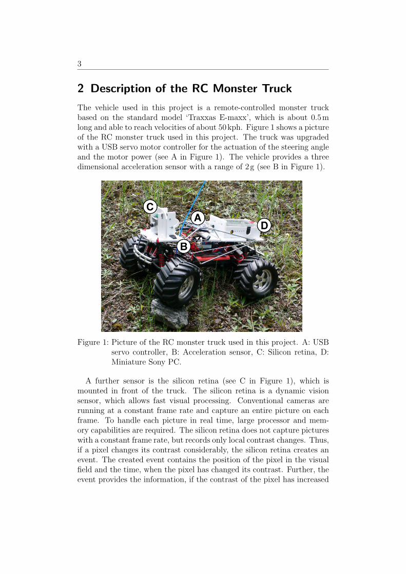
The vehicle used in this project is a remote-controlled monster truckbased on the standard model ‘Traxxas E-maxx’, which is about 0.5mlong and able to reach velocities of about 50kph. Figure 1 shows a pictureof the RC monster truck used in this project. The truck was upgradedwith a USB servo motor controller for the actuation of the steering angleand the motor power (see A in Figure 1). The vehicle provides a threedimensional acceleration sensor with a range of 2g (see B in Figure 1).
Figure 1: Picture of the RC monster truck used in this project. A: USBservo controller, B: Acceleration sensor, C: Silicon retina, D:Miniature Sony PC.
A further sensor is the silicon retina (see C in Figure 1), which ismounted in front of the truck. The silicon retina is a dynamic visionsensor, which allows fast visual processing. Conventional cameras arerunning at a constant frame rate and capture an entire picture on eachframe. To handle each picture in real time, large processor and mem-ory capabilities are required. The silicon retina does not capture pictureswith a constant frame rate, but records only local contrast changes. Thus,if a pixel changes its contrast considerably, the silicon retina creates anevent. The created event contains the position of the pixel in the visualfield and the time, when the pixel has changed its contrast. Further, theevent provides the information, if the contrast of the pixel has increased
4
or decreased. These events are called spikes, so the output of the sili-con retina are spike packages, containing information about the contrastchange of the different pixels in the visual field. The spikes of the siliconretina are handled by jAER. jAER is a Java-based package for fast visualprocessing with spikes. In this project, jAER runs on a miniature SonyPC, which is mounted on the RC monster truck (see D in Figure 1). Thecontrol policy and the filter, which handles the spikes to detect the road,are implemented in jAER on the embedded PC. The embedded PC isconnected with the sensors and the USB servo motor controller throughUSB cables.
5
3 Modeling the RC Monster Truck
In order to implement a realistic simulation of the vehicle dynamics andfurther to design a controller for the truck, it is necessary to identifymodels of different complexity. The models should include all relevantdynamics of the RC monster truck, but at the same time there are restric-tions on the complexity, because otherwise the calculation effort raisestoo much.
3.1 Assumptions
In the following, the basic assumptions which are made for the identifi-cation of the complex model are explained.
For the modeling, the RC monster truck is divided into a rigid bodyand four wheels, which are coupled to the body by the suspensions. Thesuspensions are assumed to consist of a spring, a damper and an inflexi-ble stick, which are fixed in a particular configuration with the body andthe wheel. The detailed configuration of these three elements will be in-troduced when we derive the suspension forces. We make the assumptionthat the center of gravity of the body is the same point as the center ofgravity of the whole vehicle. Further, we assume that we can directly setthe driving torque and the steering angle without any delay.
We define a local coordinate system, which moves with the truck. Theaxes of the local coordinate system are denoted with lower case letters,while the axes of the inertial coordinate system are denoted with uppercase letters. The x-axis of the local coordinate system targets always inforward direction of the vehicle and the z-axis, defined as the axis normalto the ground, keeps always the direction of the inertial Z-axis. Hence,the local coordinate system turns around the z-axis when the truck drivesthrough a curve. The center of the local coordinate system is the centerof gravity of the body. If the body turns around the x-axis or around they-axis, the local coordinate system does not follow, otherwise the z-axiswould no longer target in the direction of the inertial Z-axis. So, thecenters of the four wheels do not move in the local coordinate system.This coordinate system is chosen because it provides the advantage thatthe longitudinal velocity of the vehicle always has the same direction asthe x-axis and the lateral velocity of the vehicle always has the samedirection as the y-axis. That simplifies the derivation of the differentialequations for the longitudinal and the lateral acceleration of the truck.
For the modeling of the rotational dynamics of the body, a furthercoordinate system, which is rigidly coupled with the body of the truck,
6 3.2 Nonlinear Model
is defined. The axes of this coordinate system are denoted by xb, yb
and zb and the center point is the same as the center point of the localvehicle coordinate system. This coordinate system allows to describe therotational dynamics of the body in a simple way.
Thus, relative to the inertial coordinate system, the vehicle coordinatesystem rotates around the Z-axis and the coordinate system rigidly cou-pled with the body rotates around all three axes. The rotation angle ofthe vehicle around the Z-axis is denoted by ϕz and the additional rota-tion angles of the body are denoted by ϕx and ϕy. We can assume thatthe angle ϕx is small and does influence the forces on the body.
Further, we assume that the silicon retina is rigidly coupled with thebody at a constant height and at constant inclination.
3.2 Nonlinear Model
For the simulation (see Section 4), a model of the truck is required thatrepresents the real dynamics of the vehicle as accurately as possible. Forthat reason, a complex model, including the suspensions and the wheeldynamics, is derived in this section.
Longitudinal Dynamics
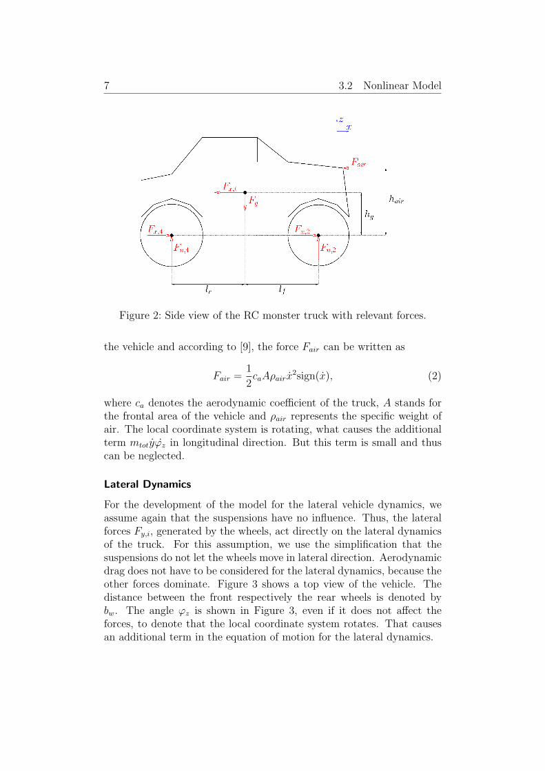
The longitudinal dynamics of the truck are considered in an externalview. We assume that the forces generated by the wheels directly affectthe truck, i.e. the influence of the suspensions is neglected. This assump-tion can be made, because the suspensions do not allow a longitudinaldeparture of the wheels related to the body. The forces generated by thewheels are denoted Fx,i, with i ∈ {1, 2, 3, 4} for each wheel. Another rel-evant force for the longitudinal dynamics of a vehicle is the aerodynamicdrag, which is assumed to act on a constant height hair. The longitudinalinert force Fx,t = mtotx acts on the center of gravity at the height hg.Figure 2 shows a side view of the truck including all relevant forces forthe longitudinal dynamics of the vehicle. The forces of the left wheelsare not drawn, but of course they have to be considered as well. Thelongitudinal position of the center of gravity is described by its distanceto the front wheels lf , respectively its distance to the rear wheels lr.
A balance of forces in longitudinal direction yields
mtotx = Fx,1 + Fx,2 + Fx,3 + Fx,4 − Fair, (1)
where the mass mtot includes the mass of the body and the mass of thefour wheels. The aerodynamic resistance Fair depends on the velocity of
7 3.2 Nonlinear Model
Figure 2: Side view of the RC monster truck with relevant forces.
the vehicle and according to [9], the force Fair can be written as
Fair =1
2caAρairx
2sign(x), (2)
where ca denotes the aerodynamic coefficient of the truck, A stands forthe frontal area of the vehicle and ρair represents the specific weight ofair. The local coordinate system is rotating, what causes the additionalterm mtotyϕz in longitudinal direction. But this term is small and thuscan be neglected.
Lateral Dynamics
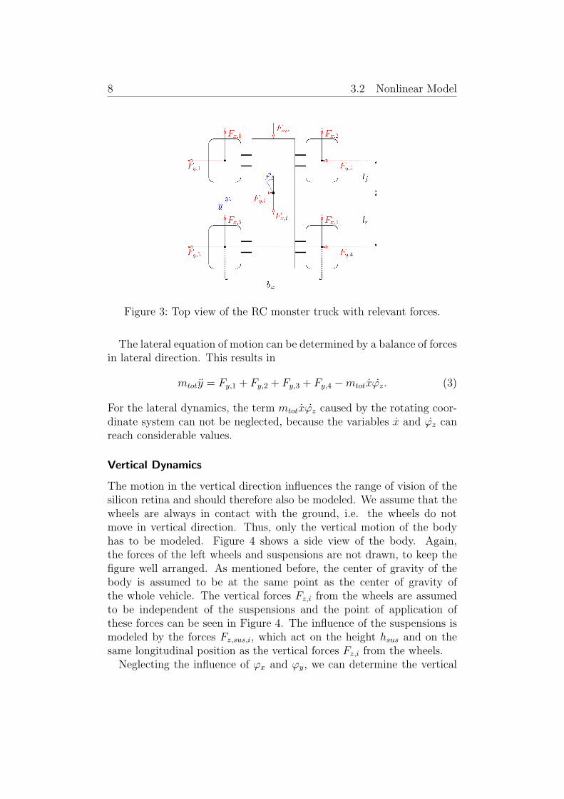
For the development of the model for the lateral vehicle dynamics, weassume again that the suspensions have no influence. Thus, the lateralforces Fy,i, generated by the wheels, act directly on the lateral dynamicsof the truck. For this assumption, we use the simplification that thesuspensions do not let the wheels move in lateral direction. Aerodynamicdrag does not have to be considered for the lateral dynamics, because theother forces dominate. Figure 3 shows a top view of the vehicle. Thedistance between the front respectively the rear wheels is denoted bybw. The angle ϕz is shown in Figure 3, even if it does not affect theforces, to denote that the local coordinate system rotates. That causesan additional term in the equation of motion for the lateral dynamics.
8 3.2 Nonlinear Model
Figure 3: Top view of the RC monster truck with relevant forces.
The lateral equation of motion can be determined by a balance of forcesin lateral direction. This results in
mtoty = Fy,1 + Fy,2 + Fy,3 + Fy,4 −mtotxϕz. (3)
For the lateral dynamics, the term mtotxϕz caused by the rotating coor-dinate system can not be neglected, because the variables x and ϕz canreach considerable values.
Vertical Dynamics
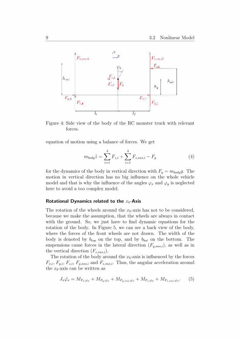
The motion in the vertical direction influences the range of vision of thesilicon retina and should therefore also be modeled. We assume that thewheels are always in contact with the ground, i.e. the wheels do notmove in vertical direction. Thus, only the vertical motion of the bodyhas to be modeled. Figure 4 shows a side view of the body. Again,the forces of the left wheels and suspensions are not drawn, to keep thefigure well arranged. As mentioned before, the center of gravity of thebody is assumed to be at the same point as the center of gravity ofthe whole vehicle. The vertical forces Fz,i from the wheels are assumedto be independent of the suspensions and the point of application ofthese forces can be seen in Figure 4. The influence of the suspensions ismodeled by the forces Fz,sus,i, which act on the height hsus and on thesame longitudinal position as the vertical forces Fz,i from the wheels.
Neglecting the influence of ϕx and ϕy, we can determine the vertical
9 3.2 Nonlinear Model
Figure 4: Side view of the body of the RC monster truck with relevantforces.
equation of motion using a balance of forces. We get
mbodyz =4∑
i=1
Fz,i +4∑
i=1
Fz,sus,i − Fg (4)
for the dynamics of the body in vertical direction with Fg = mbodyg. Themotion in vertical direction has no big influence on the whole vehiclemodel and that is why the influence of the angles ϕx and ϕy is neglectedhere to avoid a too complex model.
Rotational Dynamics related to the xb-Axis
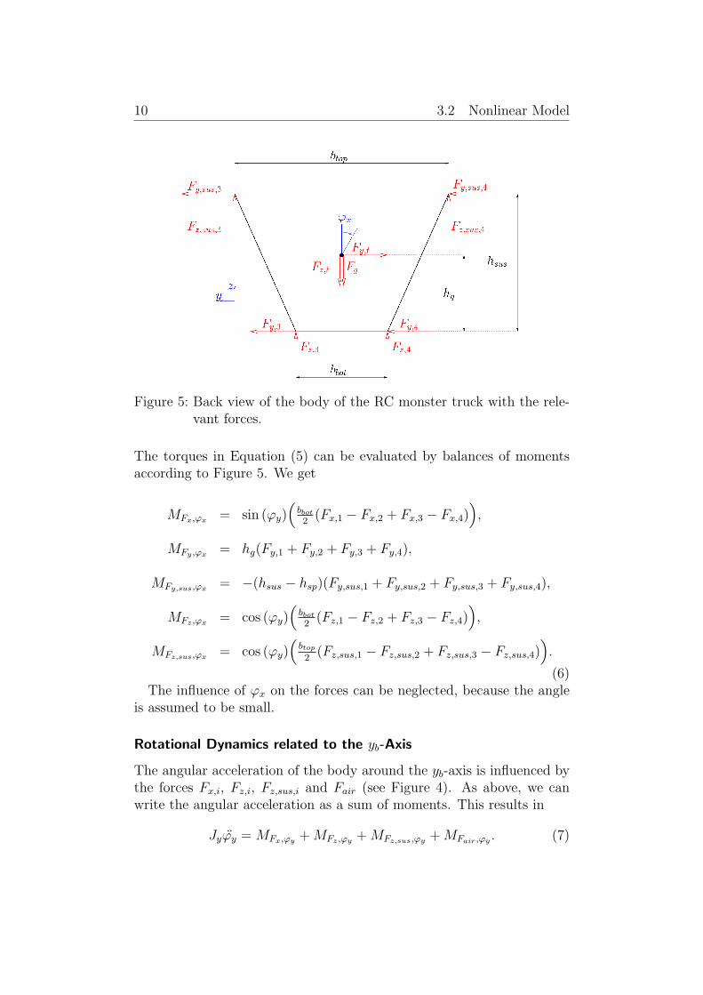
The rotation of the wheels around the xb-axis has not to be considered,because we make the assumption, that the wheels are always in contactwith the ground. So, we just have to find dynamic equations for therotation of the body. In Figure 5, we can see a back view of the body,where the forces of the front wheels are not drawn. The width of thebody is denoted by btop on the top, and by bbot on the bottom. Thesuspensions cause forces in the lateral direction (Fy,sus,i), as well as inthe vertical direction (Fz,sus,i).
The rotation of the body around the xb-axis is influenced by the forcesFx,i, Fy,i, Fz,i, Fy,sus,i and Fz,sus,i. Thus, the angular acceleration aroundthe xb-axis can be written as
Jxϕx = MFx,ϕx + MFy ,ϕx + MFy,sus,ϕx + MFz ,ϕx + MFz,sus,ϕx . (5)
10 3.2 Nonlinear Model
Figure 5: Back view of the body of the RC monster truck with the rele-vant forces.
The torques in Equation (5) can be evaluated by balances of momentsaccording to Figure 5. We get
MFx,ϕx = sin (ϕy)(
bbot
2(Fx,1 − Fx,2 + Fx,3 − Fx,4)
),
MFy ,ϕx = hg(Fy,1 + Fy,2 + Fy,3 + Fy,4),
MFy,sus,ϕx = −(hsus − hsp)(Fy,sus,1 + Fy,sus,2 + Fy,sus,3 + Fy,sus,4),
MFz ,ϕx = cos (ϕy)(
bbot
2(Fz,1 − Fz,2 + Fz,3 − Fz,4)
),
MFz,sus,ϕx = cos (ϕy)(
btop
2(Fz,sus,1 − Fz,sus,2 + Fz,sus,3 − Fz,sus,4)
).
(6)The influence of ϕx on the forces can be neglected, because the angle
is assumed to be small.
Rotational Dynamics related to the yb-Axis
The angular acceleration of the body around the yb-axis is influenced bythe forces Fx,i, Fz,i, Fz,sus,i and Fair (see Figure 4). As above, we canwrite the angular acceleration as a sum of moments. This results in
Jyϕy = MFx,ϕy + MFz ,ϕy + MFz,sus,ϕy + MFair,ϕy . (7)
11 3.2 Nonlinear Model
The calculation of the torques is not trivial, because the lever arms of theforces depend on the angle ϕy. For the calculation of the torque MFx,ϕy ,we define hx,12 as the lever arm of the forces Fx,1 and Fx,2, respectivelyhx,34 as the lever arm of the forces Fx,3 and Fx,4. Using these definitions,the moment MFx,ϕy can be written as
MFx,ϕy = hx,12(Fx,1 + Fx,2) + hx,34(Fx,3 + Fx,4), (8)
where hx,12 = fhx,12(ϕy) and hx,34 = fhx,34(ϕy) are functions of the angleϕy. Through geometrical considerations, the functions fhx,12(ϕy) andfhx,34(ϕy) can be established. The square of the maximum lever arm ofthe forces Fx,1 and Fx,2 is l2f + h2
g (see Figure 4) and for ϕy = 0 the
angular displacement of the lever arm is equal to arctan (hg
lf). Thus, the
lever arm for the forces Fx,1 and Fx,2 can be written as
hx,12 = cos
(arctan
(hg
lf
)+ ϕy
)√l2f + h2
g. (9)
Using the same considerations, it can be shown that the lever arm of theforces Fx,3 and Fx,4 is given by
hx,34 = cos
(arctan
(hg
lr
)− ϕy
)√l2r + h2
g. (10)
For the calculation of the lever arms for the forces Fz,i and Fs,sus,i, weassume that the angular displacement of the maximum lever arm is zeroand that the maximum lever arm is lr respectively lf . This assumptioncan be made, because the height of the center of gravity hg is small,relative to the length of the body lr + lf . Hence, the torque MFz ,ϕy isgiven by
MFz ,ϕy = cos (ϕy)(lr(Fz,3 + Fz,4)− lf (Fz,1 + Fz,2)
)(11)
and the torque MFz,sus,ϕy can be written as
MFz,sus,ϕy = cos (ϕy)(lr(Fz,sus,3 + Fz,sus,4)− lf (Fz,sus,1 + Fz,sus,2)
). (12)
The last moment to derive for the angular acceleration around the yb-axisis MFair,ϕy , which can be written as
MFair,ϕy = hFairFair, (13)
where the lever arm hFair= fhFair
(ϕy) also depends on the angle ϕy andcan be calculated in the same way as the lever arms hx,12 and hx,34 before.This yields in
hFair= cos
(arctan
(hair − hg
lf
)− ϕy
)√l2f + (hair − hg)2. (14)

12 3.2 Nonlinear Model
Rotational Dynamics related to the z-Axis
The part of the model for the rotational dynamics around the z-axis hasto include the entire vehicle, because not only the body rotates in thisdirection, but also the wheels. Therefore, we consider an external viewon the vehicle while we establish the following equations. According toFigure 3, the balance of moments yields in
Jzϕz = MFx,ϕz + MFy ,ϕz . (15)
In this case, the lever arms are constant and the torque caused by thelongitudinal forces Fx,i is given by
MFx,ϕz =bw
2(−Fx,1 + Fx,2 − Fx,3 + Fx,4). (16)
Further, the torque due to the lateral forces Fy,i can be written as
MFy ,ϕz = lf (Fy,1 + Fy,2)− lr(Fy,3 + Fy,4). (17)
Wheel Dynamics
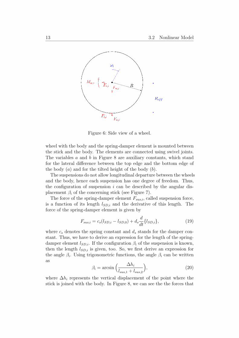
The rotational speed of the wheels highly influences the tire forces andthat is why the wheel dynamics need to be modeled for a good simulation.Figure 6 shows a wheel from the side. Fr,i denotes the rolling frictionand has no influence on the rotational speed ωi, because its point ofapplication is the center of the wheel. The radius R of the wheel is notconstant because of elastic deformation. The relevant radius for the leverarm of the longitudinal tire force Fl,i is denoted by Reff .
The only forces, which have influence on the rotational speed of thewheels, are the tire force Fl,i in direction of the related wheel and thedriving power force. The driving power is modeled as a torque Mw,i,which acts directly on the wheel. Hence, the differential equation for theangular wheel acceleration is
Jwωi = Mw,i −ReffFl,i. (18)
Suspension Forces
The dynamic equations contain the suspension forces Fy,sus,i and Fz,sus,i,so they have to be derived. The suspensions are modeled as an inelasticstick and a spring-damper element. Figure 8 shows the configurationof the suspension, the body and a wheel. The stick couples the related
13 3.2 Nonlinear Model
Figure 6: Side view of a wheel.
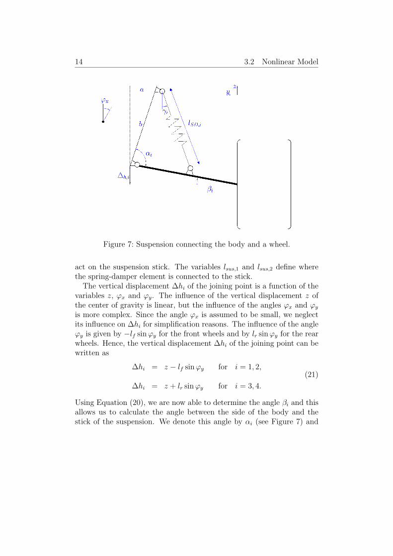
wheel with the body and the spring-damper element is mounted betweenthe stick and the body. The elements are connected using swivel joints.The variables a and b in Figure 8 are auxiliary constants, which standfor the lateral difference between the top edge and the bottom edge ofthe body (a) and for the tilted height of the body (b).
The suspensions do not allow longitudinal departure between the wheelsand the body, hence each suspension has one degree of freedom. Thus,the configuration of suspension i can be described by the angular dis-placement βi of the concerning stick (see Figure 7).
The force of the spring-damper element Fsus,i, called suspension force,is a function of its length lSD,i and the derivative of this length. Theforce of the spring-damper element is given by
Fsus,i = cs(lSD,i − lSD,0) + dsd
dt{lSD,i}, (19)
where cs denotes the spring constant and ds stands for the damper con-stant. Thus, we have to derive an expression for the length of the spring-damper element lSD,i. If the configuration βi of the suspension is known,then the length lSD,i is given, too. So, we first derive an expression forthe angle βi. Using trigonometric functions, the angle βi can be writtenas
βi = arcsin( ∆hi
lsus,1 + lsus,2
), (20)
where ∆hi represents the vertical displacement of the point where thestick is joined with the body. In Figure 8, we can see the the forces that
14 3.2 Nonlinear Model
Figure 7: Suspension connecting the body and a wheel.
act on the suspension stick. The variables lsus,1 and lsus,2 define wherethe spring-damper element is connected to the stick.
The vertical displacement ∆hi of the joining point is a function of thevariables z, ϕx and ϕy. The influence of the vertical displacement z ofthe center of gravity is linear, but the influence of the angles ϕx and ϕy
is more complex. Since the angle ϕx is assumed to be small, we neglectits influence on ∆hi for simplification reasons. The influence of the angleϕy is given by −lf sin ϕy for the front wheels and by lr sin ϕy for the rearwheels. Hence, the vertical displacement ∆hi of the joining point can bewritten as
∆hi = z − lf sin ϕy for i = 1, 2,
∆hi = z + lr sin ϕy for i = 3, 4.
(21)
Using Equation (20), we are now able to determine the angle βi and thisallows us to calculate the angle between the side of the body and thestick of the suspension. We denote this angle by αi (see Figure 7) and
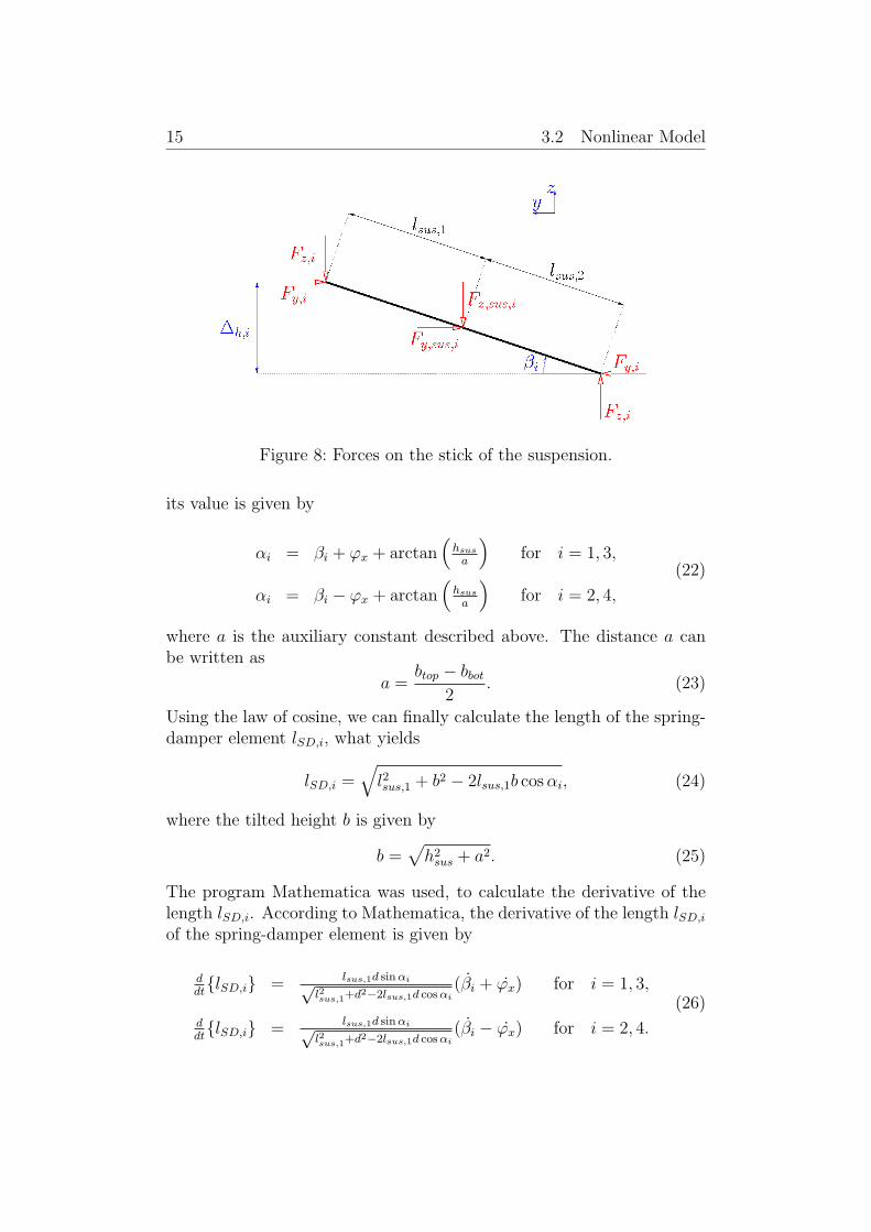
15 3.2 Nonlinear Model
Figure 8: Forces on the stick of the suspension.
its value is given by
αi = βi + ϕx + arctan(
hsus
a
)for i = 1, 3,
αi = βi − ϕx + arctan(
hsus
a
)for i = 2, 4,
(22)
where a is the auxiliary constant described above. The distance a canbe written as
a =btop − bbot
2. (23)
Using the law of cosine, we can finally calculate the length of the spring-damper element lSD,i, what yields
lSD,i =√
l2sus,1 + b2 − 2lsus,1b cos αi, (24)
where the tilted height b is given by
b =√
h2sus + a2. (25)
The program Mathematica was used, to calculate the derivative of thelength lSD,i. According to Mathematica, the derivative of the length lSD,i
of the spring-damper element is given by
ddt{lSD,i} = lsus,1d sin αi√
l2sus,1+d2−2lsus,1d cos αi(βi + ϕx) for i = 1, 3,
ddt{lSD,i} = lsus,1d sin αi√
l2sus,1+d2−2lsus,1d cos αi(βi − ϕx) for i = 2, 4.
(26)
16 3.2 Nonlinear Model
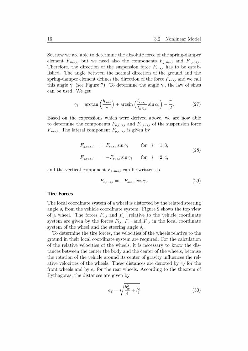
So, now we are able to determine the absolute force of the spring-damperelement Fsus,i, but we need also the components Fy,sus,i and Fz,sus,i.Therefore, the direction of the suspension force Fsus,i has to be estab-lished. The angle between the normal direction of the ground and thespring-damper element defines the direction of the force Fsus,i and we callthis angle γi (see Figure 7). To determine the angle γi, the law of sinescan be used. We get
γi = arctan(hsus
c
)+ arcsin
( lsus,1
lSD,i
sin αi
)− π
2. (27)
Based on the expressions which were derived above, we are now ableto determine the components Fy,sus,i and Fz,sus,i of the suspension forceFsus,i. The lateral component Fy,sus,i is given by
Fy,sus,i = Fsus,i sin γi for i = 1, 3,
Fy,sus,i = −Fsus,i sin γi for i = 2, 4,
(28)
and the vertical component Fz,sus,i can be written as
Fz,sus,i = −Fsus,i cos γi. (29)
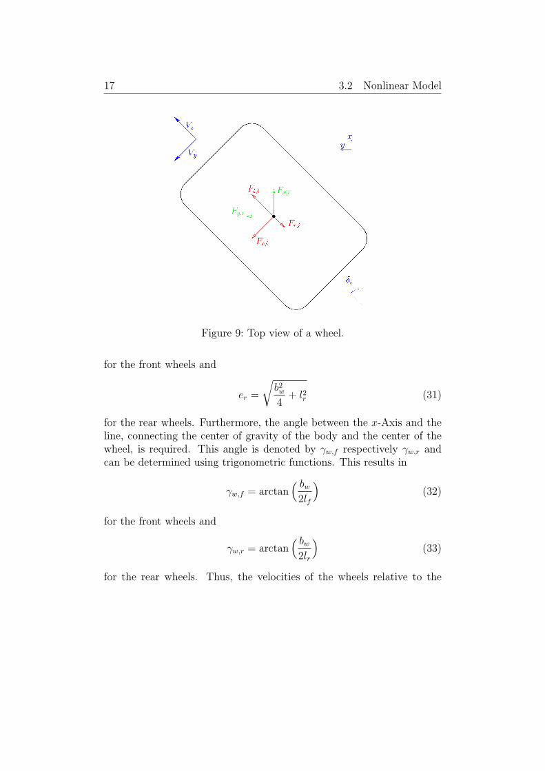
Tire Forces
The local coordinate system of a wheel is distorted by the related steeringangle δi from the vehicle coordinate system. Figure 9 shows the top viewof a wheel. The forces Fx,i and Fy,i relative to the vehicle coordinatesystem are given by the forces Fl,i, Fc,i and Fr,i in the local coordinatesystem of the wheel and the steering angle δi.
To determine the tire forces, the velocities of the wheels relative to theground in their local coordinate system are required. For the calculationof the relative velocities of the wheels, it is necessary to know the dis-tances between the center the body and the center of the wheels, becausethe rotation of the vehicle around its center of gravity influences the rel-ative velocities of the wheels. These distances are denoted by ef for thefront wheels and by er for the rear wheels. According to the theorem ofPythagoras, the distances are given by
ef =
√b2w
4+ l2f (30)
17 3.2 Nonlinear Model
Figure 9: Top view of a wheel.
for the front wheels and
er =
√b2w
4+ l2r (31)
for the rear wheels. Furthermore, the angle between the x-Axis and theline, connecting the center of gravity of the body and the center of thewheel, is required. This angle is denoted by γw,f respectively γw,r andcan be determined using trigonometric functions. This results in
γw,f = arctan( bw
2lf
)(32)
for the front wheels and
γw,r = arctan( bw
2lr
)(33)
for the rear wheels. Thus, the velocities of the wheels relative to the
18 3.2 Nonlinear Model
ground in the vehicle coordinate system are given by
vx,1 = x− ef ϕz sin γw,f ,
vx,2 = x + ef ϕz sin γw,f ,
vx,3 = x− erϕz sin γw,r,
vx,4 = x + erϕz sin γw,r,
(34)
in the forward direction, i.e. in the direction of the x-axis. Further, weget
vy,1 = y + ef ϕz cos γw,f ,
vy,2 = y + ef ϕz cos γw,f ,
vy,3 = y − erϕz cos γw,r,
vy,4 = y − erϕz cos γw,r,
(35)
for the lateral direction. Considering the steering angles δi and usingthe Equations (34) and (35), the velocities of the wheels relative to theground in their local coordinate system become
Vx,1 = cos δ1(x− ef ϕz sin γw,f ) + sin δ1(y + ef ϕz cos γw,f ),
Vx,2 = cos δ2(x + ef ϕz sin γw,f ) + sin δ2(y + ef ϕz cos γw,f ),
Vx,3 = cos δ3(x− erϕz sin γw,r) + sin δ3(y − erϕz cos γw,r),
Vx,4 = cos δ4(x + erϕz sin γw,r) + sin δ4(y − erϕz cos γw,r),
(36)
in the longitudinal direction and
Vy,1 = − sin δ1(x− ef ϕz sin γw,f ) + cos δ1(y + ef ϕz cos γw,f ),
Vy,2 = − sin δ2(x + ef ϕz sin γw,f ) + cos δ2(y + ef ϕz cos γw,f ),
Vy,3 = − sin δ3(x− erϕz sin γw,r) + cos δ3(y − erϕz cos γw,r),
Vy,4 = − sin δ4(x + erϕz sin γw,r) + cos δ4(y − erϕz cos γw,r),
(37)

19 3.2 Nonlinear Model
in the lateral direction. The cornering forces Fc,i are the forces generatedby the wheels in the local lateral direction, i.e. in the direction of thevelocity Vy,i. The slip angles of the tires are assumed to be small, becausethen the cornering force Fc,i of each wheel is proportional to the slipangle. In this case, according to [9], the cornering force Fc,i of a tire canbe written as
Fc,i = Cα
(δi −
Vy,i
Vx,i
), (38)
where Cα represents the constant cornering stiffness of the tire. Thelongitudinal slip ratio is also assumed to be small, hence the longitudinaltire force Fl,i is proportional to the slip ratio and can, according to [9],be written as
Fl,i = Cσ
(Reffωi − Vx,i
Reffωi
)(39)
during acceleration and
Fl,i = Cσ
(Reffωi − Vx,i
Vx,i
)(40)
during braking. The constant Cσ stands for the longitudinal tire stiffness.The elasticity of the tires causes the rolling friction force Fr,i, which canbe calculated by
Fr,i = CrFn,isign(Vx,i), (41)
as shown in [9]. The rolling friction force Fr,i has to be subtracted fromthe longitudinal tire force Fl,i. The forces generated by the tire in the ve-hicle coordinate system, denoted by Fx,i and Fy,i, have now been derivedand are given by
Fx,i = (Fl,i − Fr,i) cos δi − Fc,i sin δi (42)
andFy,i = (Fl,i − Fr,i) sin δi + Fc,i cos δi. (43)
Normal Forces
For the calculation of the normal forces on the tires, we neglect theinfluence of the angles ϕx and ϕy. Using this assumption, the normalforces can be written as
Fn,i =lr
2(lf + lr)mtotg + Fdyn,i (44)
20 3.3 Reduced Model for Controller Design
for the front wheels and
Fn,i =lf
2(lf + lr)mtotg + Fdyn,i (45)
for the rear wheels. The dynamic terms Fdyn,i are caused by the longitu-dinal acceleration x, the lateral acceleration y and the aerodynamic dragFair. The forces Fdyn,i can be established with balances of moments onthe vehicle x-axis and on the vehicle y-axis. This yields in
Fdyn,1 = −Fairhair+mtotx2(lf+lr)
− mtoty2bw
,
Fdyn,2 = −Fairhair+mtotx2(lf+lr)
+ mtoty2bw
,
Fdyn,3 = Fairhair+mtotx2(lf+lr)
− mtoty2bw
,
Fdyn,4 = Fairhair+mtotx2(lf+lr)
+ mtoty2bw
.
(46)
The constant bw stands for the width of the vehicle, i.e. for the distancebetween the center of two opposite wheels (see figure 3). To get the nor-mal forces Fz,i on the body, the weight of the wheels has to be subtractedfrom the normal forces Fn,i on the tires. Thus, we get
Fz,i = Fn,i −mwg. (47)
Silicon Retina
Even if the silicon retina does not influence the dynamics of the truck,it is important to know its position and orientation to place it correctlyin the virtual model. The silicon retina is rigidly coupled with the bodyof the truck at a constant height hsr. The orientation has an angulardisplacement of ϕsr to the xb-axis, while using yb as the rotating axis.
3.3 Reduced Model for Controller Design
To get a realistic simulation in Blender, it was necessary to model allstates which influence the view of the silicon retina considerably. But forcontroller design, a model consisting of less dynamic states is advanta-geous. Therefore, the complex model of the truck has to be simplified.
21 3.3 Reduced Model for Controller Design
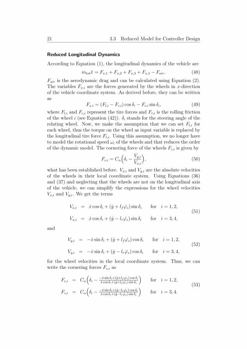
Reduced Longitudinal Dynamics
According to Equation (1), the longitudinal dynamics of the vehicle are
mtotx = Fx,1 + Fx,2 + Fx,3 + Fx,4 − Fair. (48)
Fair is the aerodynamic drag and can be calculated using Equation (2).The variables Fx,i are the forces generated by the wheels in x-directionof the vehicle coordinate system. As derived before, they can be writtenas
Fx,i = (Fl,i − Fr,i) cos δi − Fc,i sin δi, (49)
where Fl,i and Fc,i represent the tire forces and Fr,i is the rolling frictionof the wheel i (see Equation (42)). δi stands for the steering angle of therelating wheel. Now, we make the assumption that we can set Fl,i foreach wheel, thus the torque on the wheel as input variable is replaced bythe longitudinal tire force Fl,i. Using this assumption, we no longer haveto model the rotational speed ωi of the wheels and that reduces the orderof the dynamic model. The cornering force of the wheels Fc,i is given by
Fc,i = Cα
(δi −
Vy,i
Vx,i
), (50)
what has been established before. Vx,i and Vy,i are the absolute velocitiesof the wheels in their local coordinate system. Using Equations (36)and (37) and neglecting that the wheels are not on the longitudinal axisof the vehicle, we can simplify the expressions for the wheel velocitiesVx,i and Vy,i. We get the terms
Vx,i = x cos δi + (y + lf ϕz) sin δi for i = 1, 2,
Vx,i = x cos δi + (y − lrϕz) sin δi for i = 3, 4,
(51)
and
Vy,i = −x sin δi + (y + lf ϕz) cos δi for i = 1, 2,
Vy,i = −x sin δi + (y − lrϕz) cos δi for i = 3, 4,
(52)
for the wheel velocities in the local coordinate system. Thus, we canwrite the cornering forces Fc,i as
Fc,i = Cα
(δi − −x sin δi+(y+lf ϕz) cos δi
x cos δi+(y+lf ϕz) sin δi
)for i = 1, 2,
Fc,i = Cα
(δi − −x sin δi+(y−lrϕz) cos δi
x cos δi+(y−lrϕz) sin δi
)for i = 3, 4.
(53)
22 3.3 Reduced Model for Controller Design
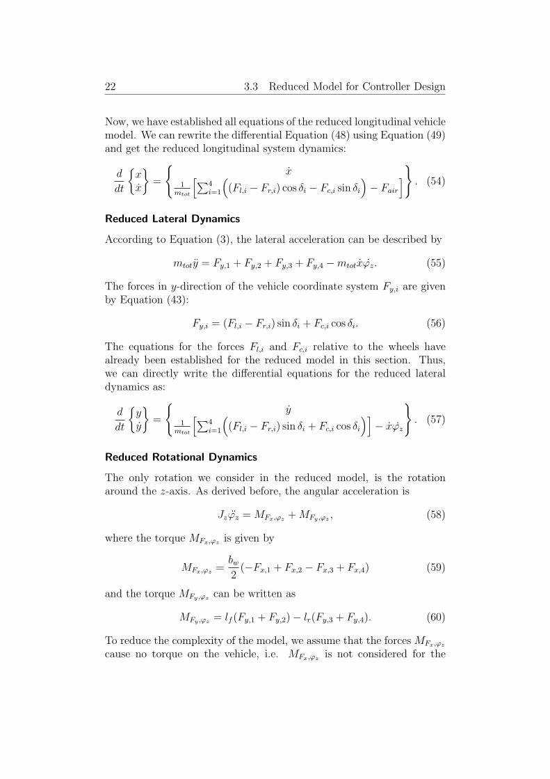
Now, we have established all equations of the reduced longitudinal vehiclemodel. We can rewrite the differential Equation (48) using Equation (49)and get the reduced longitudinal system dynamics:
d
dt
{xx
}=
{x
1mtot
[∑4i=1
((Fl,i − Fr,i) cos δi − Fc,i sin δi
)− Fair
]}. (54)
Reduced Lateral Dynamics
According to Equation (3), the lateral acceleration can be described by
mtoty = Fy,1 + Fy,2 + Fy,3 + Fy,4 −mtotxϕz. (55)
The forces in y-direction of the vehicle coordinate system Fy,i are givenby Equation (43):
Fy,i = (Fl,i − Fr,i) sin δi + Fc,i cos δi. (56)
The equations for the forces Fl,i and Fc,i relative to the wheels havealready been established for the reduced model in this section. Thus,we can directly write the differential equations for the reduced lateraldynamics as:
d
dt
{yy
}=
{y
1mtot
[∑4i=1
((Fl,i − Fr,i) sin δi + Fc,i cos δi
)]− xϕz
}. (57)
Reduced Rotational Dynamics
The only rotation we consider in the reduced model, is the rotationaround the z-axis. As derived before, the angular acceleration is
Jzϕz = MFx,ϕz + MFy ,ϕz , (58)
where the torque MFx,ϕz is given by
MFx,ϕz =bw
2(−Fx,1 + Fx,2 − Fx,3 + Fx,4) (59)
and the torque MFy ,ϕz can be written as
MFy ,ϕz = lf (Fy,1 + Fy,2)− lr(Fy,3 + Fy,4). (60)
To reduce the complexity of the model, we assume that the forces MFx,ϕz
cause no torque on the vehicle, i.e. MFx,ϕz is not considered for the
23 3.3 Reduced Model for Controller Design
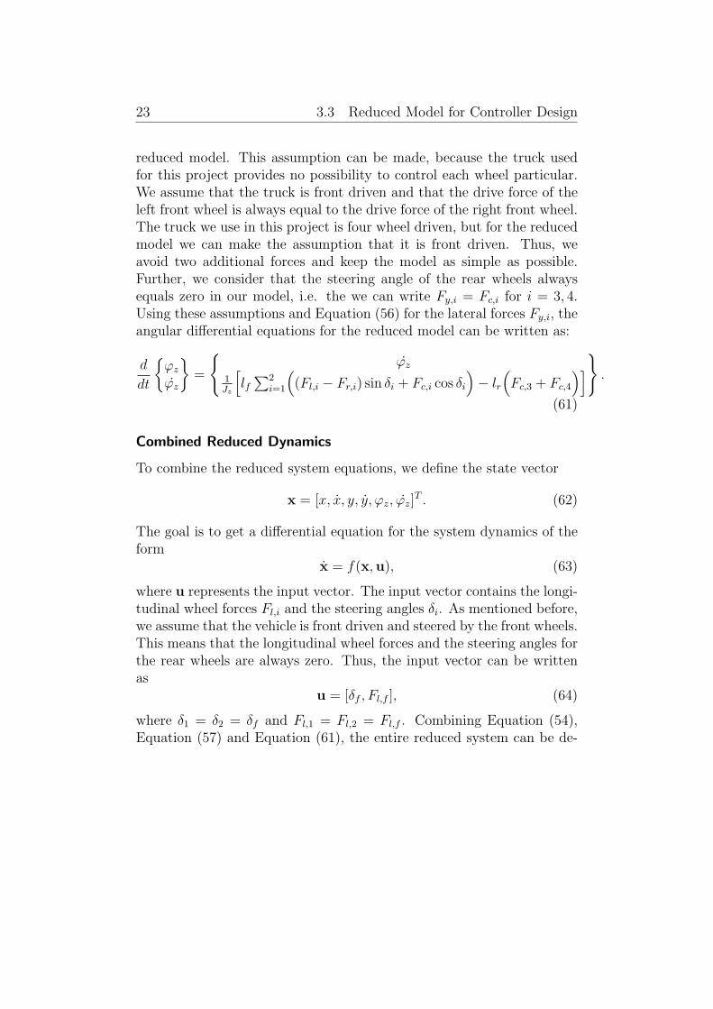
reduced model. This assumption can be made, because the truck usedfor this project provides no possibility to control each wheel particular.We assume that the truck is front driven and that the drive force of theleft front wheel is always equal to the drive force of the right front wheel.The truck we use in this project is four wheel driven, but for the reducedmodel we can make the assumption that it is front driven. Thus, weavoid two additional forces and keep the model as simple as possible.Further, we consider that the steering angle of the rear wheels alwaysequals zero in our model, i.e. the we can write Fy,i = Fc,i for i = 3, 4.Using these assumptions and Equation (56) for the lateral forces Fy,i, theangular differential equations for the reduced model can be written as:
d
dt
{ϕz
ϕz
}=
{ϕz
1Jz
[lf
∑2i=1
((Fl,i − Fr,i) sin δi + Fc,i cos δi
)− lr
(Fc,3 + Fc,4
)]}.
(61)
Combined Reduced Dynamics
To combine the reduced system equations, we define the state vector
x = [x, x, y, y, ϕz, ϕz]T . (62)
The goal is to get a differential equation for the system dynamics of theform
x = f(x,u), (63)
where u represents the input vector. The input vector contains the longi-tudinal wheel forces Fl,i and the steering angles δi. As mentioned before,we assume that the vehicle is front driven and steered by the front wheels.This means that the longitudinal wheel forces and the steering angles forthe rear wheels are always zero. Thus, the input vector can be writtenas
u = [δf , Fl,f ], (64)
where δ1 = δ2 = δf and Fl,1 = Fl,2 = Fl,f . Combining Equation (54),Equation (57) and Equation (61), the entire reduced system can be de-
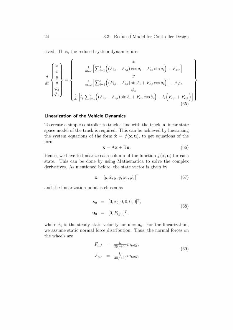
24 3.3 Reduced Model for Controller Design
rived. Thus, the reduced system dynamics are:
d
dt
xxyyϕz
ϕz
=
x1
mtot
[∑4i=1
((Fl,i − Fr,i) cos δi − Fc,i sin δi
)− Fair
]y
1mtot
[∑4i=1
((Fl,i − Fr,i) sin δi + Fc,i cos δi
)]− xϕz
ϕz
1Jz
[lf
∑2i=1
((Fl,i − Fr,i) sin δi + Fc,i cos δi
)− lr
(Fc,3 + Fc,4
)]
.
(65)
Linearization of the Vehicle Dynamics
To create a simple controller to track a line with the truck, a linear statespace model of the truck is required. This can be achieved by linearizingthe system equations of the form x = f(x,u), to get equations of theform
x = Ax + Bu. (66)
Hence, we have to linearize each column of the function f(x,u) for eachstate. This can be done by using Mathematica to solve the complexderivatives. As mentioned before, the state vector is given by
x = [y, x, y, y, ϕz, ϕz]T (67)
and the linearization point is chosen as
x0 = [0, x0, 0, 0, 0, 0]T ,
u0 = [0, Fl,f,0]T ,
(68)
where x0 is the steady state velocity for u = u0. For the linearization,we assume static normal force distribution. Thus, the normal forces onthe wheels are
Fn,f = lr2(lf+lr)
mtotg,
Fn,r =lf
2(lf+lr)mtotg,
(69)
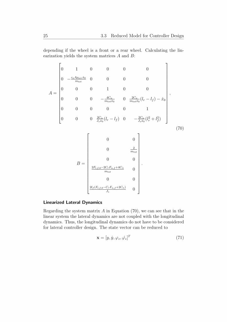
25 3.3 Reduced Model for Controller Design
depending if the wheel is a front or a rear wheel. Calculating the lin-earization yields the system matrices A and B:
A =
0 1 0 0 0 0
0 − caAρairx0
mtot0 0 0 0
0 0 0 1 0 0
0 0 0 − 4Cα
mtotx00 2Cα
mtotx0(lr − lf )− x0
0 0 0 0 0 1
0 0 0 2Cα
Jz x0(lr − lf ) 0 − 2Cα
Jz x0(l2r + l2f )
,
B =
0 0
0 2mtot
0 0
2Fl,f,0−2CrFn,f+4Cα
mtot0
0 0
2lf (Fl,f,0−CrFn,f+2Cα)
Jz0
.
(70)
Linearized Lateral Dynamics
Regarding the system matrix A in Equation (70), we can see that in thelinear system the lateral dynamics are not coupled with the longitudinaldynamics. Thus, the longitudinal dynamics do not have to be consideredfor lateral controller design. The state vector can be reduced to
x = [y, y, ϕz, ϕz]T (71)
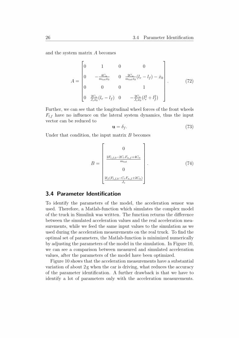
26 3.4 Parameter Identification
and the system matrix A becomes
A =
0 1 0 0
0 − 4Cα
mtotx00 2Cα
mtotx0(lr − lf )− x0
0 0 0 1
0 2Cα
Jz x0(lr − lf ) 0 − 2Cα
Jz x0(l2r + l2f )
. (72)
Further, we can see that the longitudinal wheel forces of the front wheelsFl,f have no influence on the lateral system dynamics, thus the inputvector can be reduced to
u = δf . (73)
Under that condition, the input matrix B becomes
B =
0
2Fl,f,0−2CrFn,f+4Cα
mtot
0
2lf (Fl,f,0−CrFn,f+2Cα)
Jz
. (74)
3.4 Parameter Identification
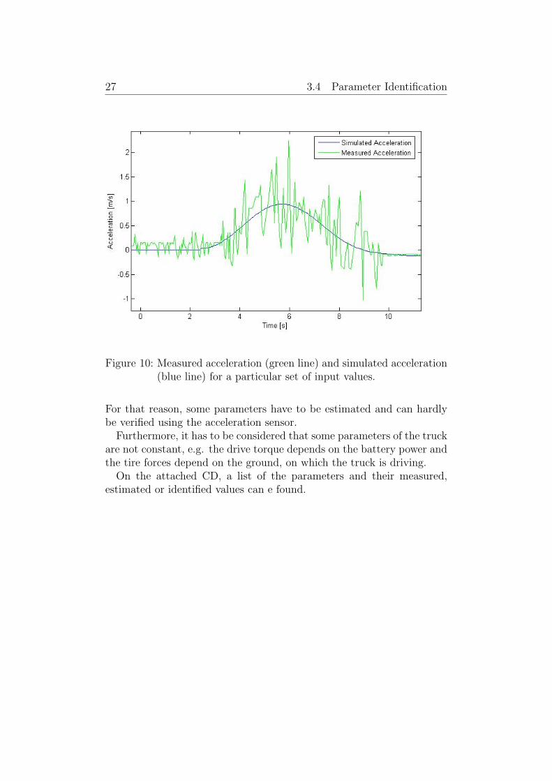
To identify the parameters of the model, the acceleration sensor wasused. Therefore, a Matlab-function which simulates the complex modelof the truck in Simulink was written. The function returns the differencebetween the simulated acceleration values and the real acceleration mea-surements, while we feed the same input values to the simulation as weused during the acceleration measurements on the real truck. To find theoptimal set of parameters, the Matlab-function is minimized numericallyby adjusting the parameters of the model in the simulation. In Figure 10,we can see a comparison between measured and simulated accelerationvalues, after the parameters of the model have been optimized.
Figure 10 shows that the acceleration measurements have a substantialvariation of about 2g when the car is driving, what reduces the accuracyof the parameter identification. A further drawback is that we have toidentify a lot of parameters only with the acceleration measurements.
27 3.4 Parameter Identification
Figure 10: Measured acceleration (green line) and simulated acceleration(blue line) for a particular set of input values.
For that reason, some parameters have to be estimated and can hardlybe verified using the acceleration sensor.
Furthermore, it has to be considered that some parameters of the truckare not constant, e.g. the drive torque depends on the battery power andthe tire forces depend on the ground, on which the truck is driving.
On the attached CD, a list of the parameters and their measured,estimated or identified values can e found.
28
4 Simulation in Blender
In order to test a particular controller for the RC monster truck, a virtualthree dimensional environment is employed, which allows to simulate thesilicon retina. Therefore, a virtual model of the vehicle with nearly thesame dynamics as the original has to be created. Blender, an open-sourceprogram for three dimensional modeling, was chosen as our test environ-ment. Blender provides the possibility to integrate Python scripts, whichallow to implement the complex dynamics of the truck.
4.1 Simulation Concept
The dynamics of the vehicle in the simulation should approximate thereal behavior of the truck as good as possible, to get a realistic testenvironment. In Section 3, a complex model of the vehicle was derived.This model contains the relevant dynamics which influence the field ofview of the silicon retina. Thus, if we are able to run the simulation basedon this model, we have the possibility to test a particular controller forthe truck including the visual part.
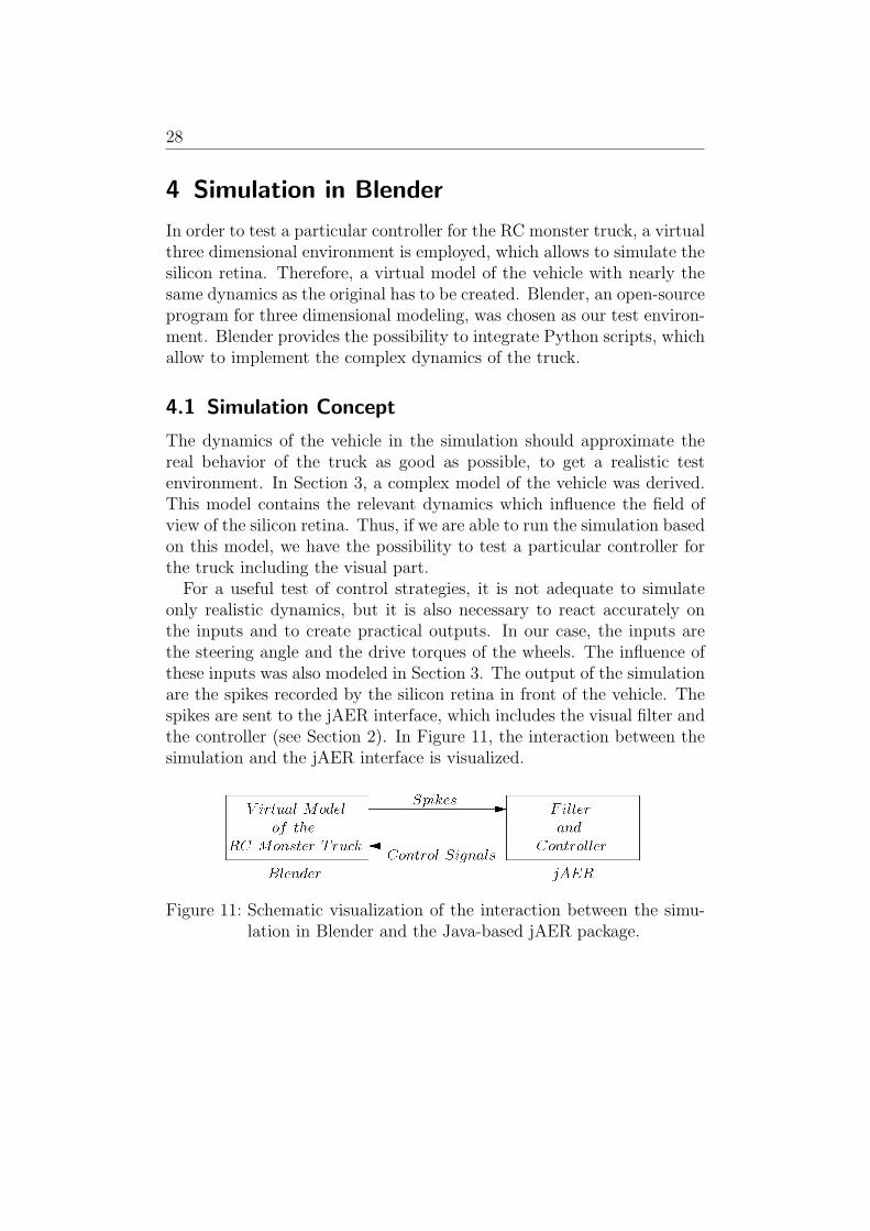
For a useful test of control strategies, it is not adequate to simulateonly realistic dynamics, but it is also necessary to react accurately onthe inputs and to create practical outputs. In our case, the inputs arethe steering angle and the drive torques of the wheels. The influence ofthese inputs was also modeled in Section 3. The output of the simulationare the spikes recorded by the silicon retina in front of the vehicle. Thespikes are sent to the jAER interface, which includes the visual filter andthe controller (see Section 2). In Figure 11, the interaction between thesimulation and the jAER interface is visualized.
Figure 11: Schematic visualization of the interaction between the simu-lation in Blender and the Java-based jAER package.

29 4.2 Implementation
4.2 Implementation
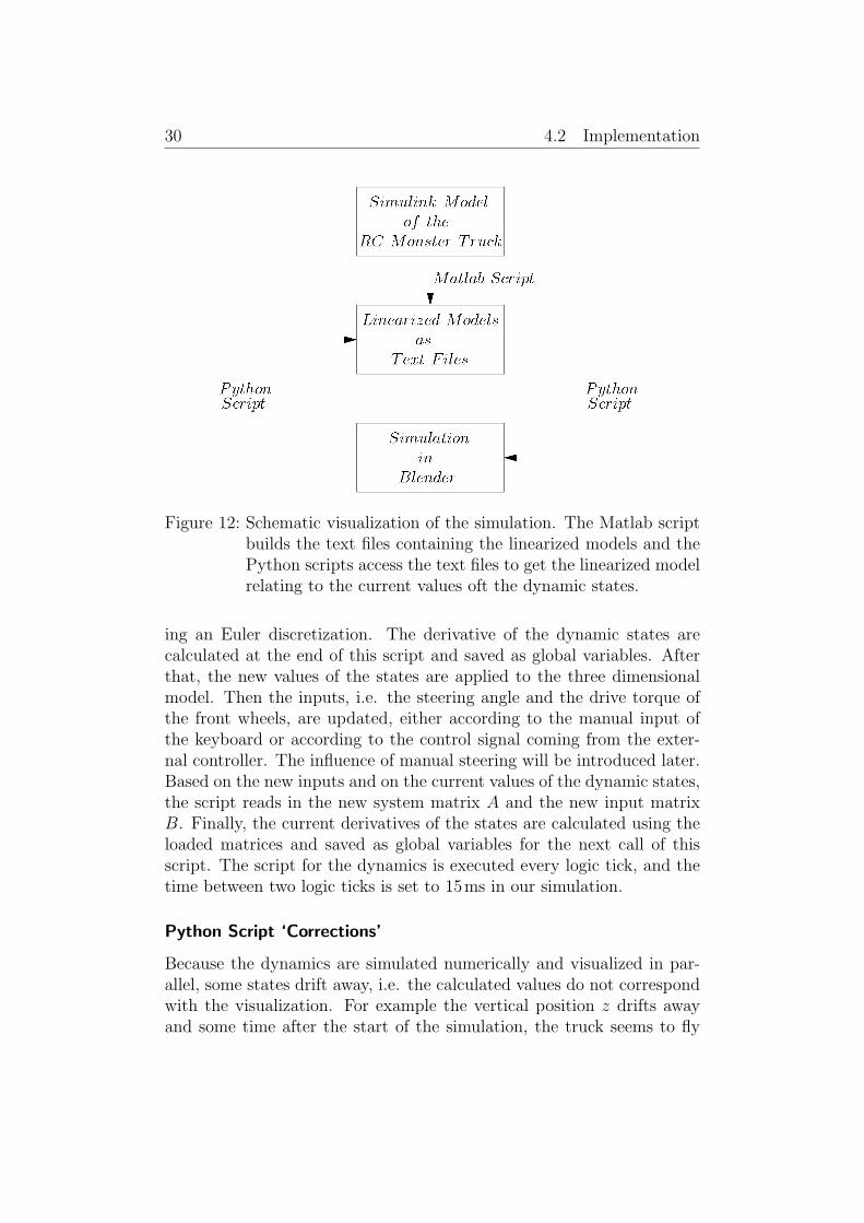
The dynamics of the vehicle are not linear and their calculation is nu-merically expensive. But the frequency of the calculation of the dynamicvariables of the model should be as high as possible, so that the qualityof the visual output is not affected by studdering. For that reason, wecreate a state mesh and linearize the complex model at each point ofthe mesh. Therefore, a Matlab script has been created, which allows tolinearize a Simulink model at each point of the user defined state mesh.This provides also the advantage that it is not needed to change thePython code in the Blender file, when we want to change the model ofthe truck. It is only necessary to modify the Simulink model and, afterexecuting the Matlab script, the simulation in Blender is adjusted to thechanges. The Matlab script builds a text file for each linearization pointand a folder containing the information about the used state mesh. Eachtext file comprehends the relating matrices A and B, which describe theconcerning linear system. The folder for the state mesh contains a textfile for each state with information about the resolution and the range ofthe related state. All text files are labeled in a defined format, so thatthe Python scripts can access the files without manual modifications.Figure 12 visualizes the handling of the linearized models.
The dynamics, which are simulated and visualized using the strategydescribed above, are the motions in all three directions, the rotationsaround all axes and the rotations of the wheels, everything relative tothe local coordinate system of the vehicle. The simulation in Blenderis based on eight separate Python scripts, which are explained in thefollowing.
Python Script ‘Initialize’
This Python script sets up the simulation environment and initializes theglobal variables. Global variables are the current values of the dynamicstates and their current derivatives, the resolution and the range of thestate mesh, and some other factors and pointers which are necessaryfor the simulation. The resolution and the range of the state mesh arecalculated using the text files created by the Matlab code. This Pythonscript is executed once when the simulation starts.
Python Script ‘Dynamics’
The Python script for the dynamics handles the motions of the virtualvehicle. First, the new values of the dynamic states are calculated us-
30 4.2 Implementation
Figure 12: Schematic visualization of the simulation. The Matlab scriptbuilds the text files containing the linearized models and thePython scripts access the text files to get the linearized modelrelating to the current values oft the dynamic states.
ing an Euler discretization. The derivative of the dynamic states arecalculated at the end of this script and saved as global variables. Afterthat, the new values of the states are applied to the three dimensionalmodel. Then the inputs, i.e. the steering angle and the drive torque ofthe front wheels, are updated, either according to the manual input ofthe keyboard or according to the control signal coming from the exter-nal controller. The influence of manual steering will be introduced later.Based on the new inputs and on the current values of the dynamic states,the script reads in the new system matrix A and the new input matrixB. Finally, the current derivatives of the states are calculated using theloaded matrices and saved as global variables for the next call of thisscript. The script for the dynamics is executed every logic tick, and thetime between two logic ticks is set to 15ms in our simulation.
Python Script ‘Corrections’
Because the dynamics are simulated numerically and visualized in par-allel, some states drift away, i.e. the calculated values do not correspondwith the visualization. For example the vertical position z drifts awayand some time after the start of the simulation, the truck seems to fly
31 4.2 Implementation
or to drop into the ground. For that reason, the python script for thecorrections is called once in ten game logic ticks. The script reads in thedrifting states from the three dimensional model and uses these valuesto adjust the numerical simulation. Another problem is that the wheelstend to drift away from the body of the truck during the simulation,also because of numerical errors. The Python script for the correctionshandles this problem as well.
Python Script ‘Settings’
During the simulation, it is possible to change between manual controland automatic control. Manual control means that the virtual vehicle iscontrolled by the keyboard arrows, while automatic control denotes thatthe vehicle is controlled by the external controller implemented in Java.Thus, we need two settings, one for steering and one for speed control.Both of these two options can be changed independently from manual toautomatic and vice versa. In the integrated command line of Blender,the inputs from the controller are always displayed during the simulation,even if the manual control mode is activated. So, it is possible to controlthe virtual truck manually and to observe at the same time, what thecontroller would do in the current situation. The Python script for thesettings is executed, whenever the user pushes one of the keys to changethe steering or the speed control mode, and handles the changing.
Python Script ‘Camera Feeder’
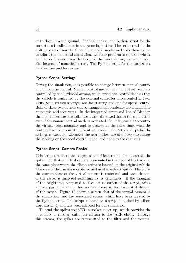
This script simulates the output of the silicon retina, i.e. it creates thespikes. For that, a virtual camera is mounted in the front of the truck, atthe same place where the silicon retina is located on the original vehicle.The view of the camera is captured and used to extract spikes. Therefore,the current view of the virtual camera is rasterized and each elementof the raster is analyzed regarding to its brightness. If the changingof the brightness, compared to the last execution of the script, raisesabove a particular value, then a spike is created for the related elementof the raster. Figure 13 shows a screen shot of the virtual camera inthe simulation, and the associated spikes, which have been created bythe Python script. This script is based on a script published by AlbertCardona in [4] and has been adapted for our simulation.
To send the spikes to jAER, a socket is set up, which provides thepossibility to send a continuous stream to the jAER client. Throughthis stream, the spikes are transmitted to the filter and the external
32 4.2 Implementation
(a) Screen shot of the three di-mensional simulation in Blender.
(b) Spikes which are generated atthe same time of the screen shot.
Figure 13: Comparison between a screen shot of the simulation in Blender(a) and the related spikes, created by a Python script (b).
controller, which are implemented in Java. This script handles also theinputs, which are transmitted through the socket stream as well, comingfrom the controller. The script decodes the input stream into the desiredsteering angle and the desired drive torque. Because the execution of thisscript is expensive in terms of calculation steps, it is only called everyfew game logic ticks, but the flow of the spikes is still sufficient.
Python Script ‘Capture Route’
To analyze the performance of a particular controller, it is advantageousto capture the driven path. Therefore, this Python script captures atrajectory which is driven during the simulation. The captured path,which consists of the position and the orientation of the truck for eachgame logic tick, is saved in a text file. This script is called every gamelogic tick, if the route capturing is activated.
Python Script ‘Rerun Captured Route’
This script allows to rerun a trajectory, which has been recorded before.If a captured path is driven again, then it is possible to switch betweendifferent views, to analyze the performance of the controller. This scriptis called every game logic tick, if the simulation is in the rerun mode.
33 4.3 Simulation Results
Python Script ‘Get Captured Route’
To test a controller without the influence of the filter which handles thespikes, this Python script determines the lateral and the angular errorsrelative to a reference route and feeds them to the controller. Thus,we assume that the filter of the silicon retina always recognizes the routeperfectly. The reference route can either be captured by the Python script‘Capture Route’, or be generated by a program, for example Matlab.
4.3 Simulation Results
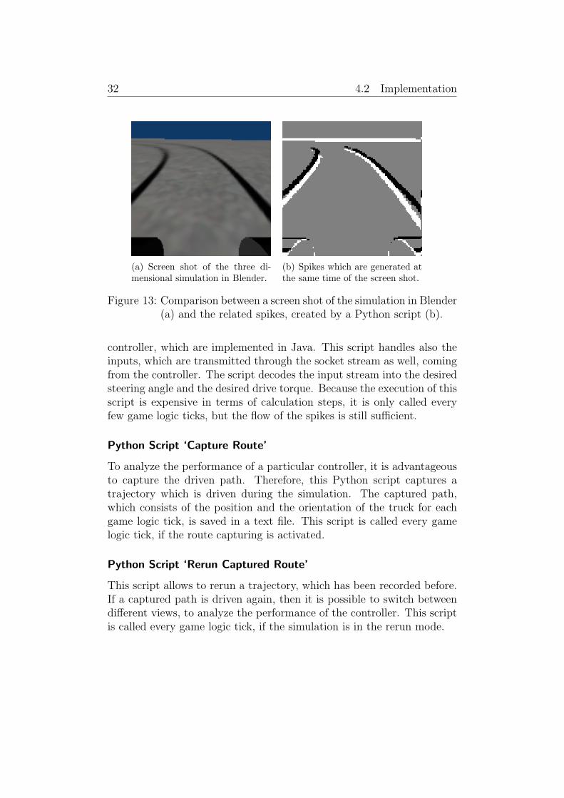
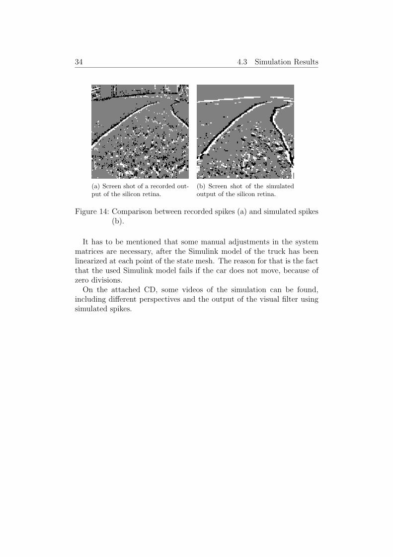
Based on the implementation introduced above, a realistic simulationof the RC monster truck can be performed, provided that we have agood model of the truck. The simulated output of the silicon retinalooks as expected. The flow of the spikes created in Blender during thesimulation is very similar to the flow of the spikes resulting from the realsilicon retina, except that the timestamps of the events are quantized tothe simulation frame rate. Depending on the texture of the ground inthe simulation, we are able to create more or less noise in the simulatedoutput of the silicon retina. Hence, the simulation provides the possibilityto test a controller under idealized conditions without noise, as well asthe possibility to test a controller under conditions which are similarto reality. Figure 14 shows a comparison between spikes which weresimulated and spikes which were recorded using the silicon retina on thetruck. In Blender, a texture with high contrast differences was chosen,what causes noise in the virtual output of the silicon retina.
34 4.3 Simulation Results
(a) Screen shot of a recorded out-put of the silicon retina.
(b) Screen shot of the simulatedoutput of the silicon retina.
Figure 14: Comparison between recorded spikes (a) and simulated spikes(b).
It has to be mentioned that some manual adjustments in the systemmatrices are necessary, after the Simulink model of the truck has beenlinearized at each point of the state mesh. The reason for that is the factthat the used Simulink model fails if the car does not move, because ofzero divisions.
On the attached CD, some videos of the simulation can be found,including different perspectives and the output of the visual filter usingsimulated spikes.
35
5 Controller Design
In this section, a controller for the lateral position of the truck is designed,based on the reduced lateral model of the system dynamics. We assumethat the silicon retina is the only available sensor and its output is filteredto get a measurement signal. The measurement signal contains the lateraldeparture of the truck relative to the middle of the route and the angulardisplacement of the vehicle relative to the direction of the route.
5.1 PID Control Scheme
The first approach we consider is to use a standard PID controller forthe lateral control of the truck.
Approach
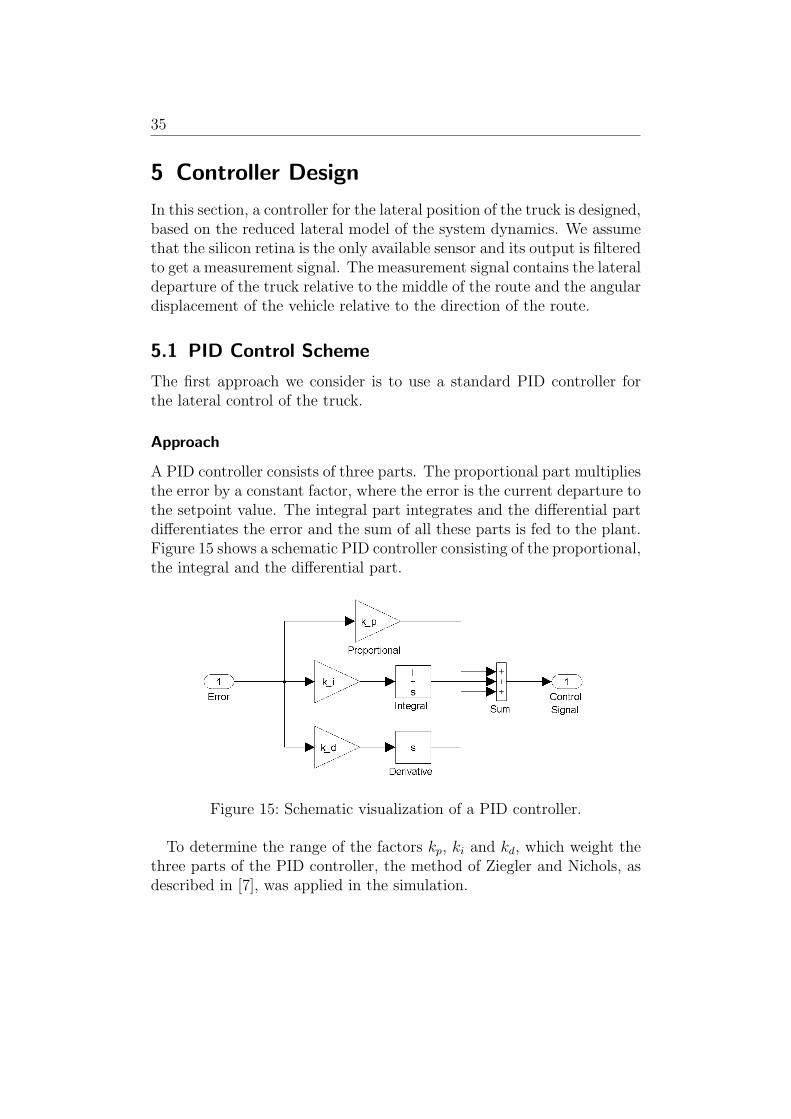
A PID controller consists of three parts. The proportional part multipliesthe error by a constant factor, where the error is the current departure tothe setpoint value. The integral part integrates and the differential partdifferentiates the error and the sum of all these parts is fed to the plant.Figure 15 shows a schematic PID controller consisting of the proportional,the integral and the differential part.
Figure 15: Schematic visualization of a PID controller.
To determine the range of the factors kp, ki and kd, which weight thethree parts of the PID controller, the method of Ziegler and Nichols, asdescribed in [7], was applied in the simulation.
36 5.1 PID Control Scheme
Implementation
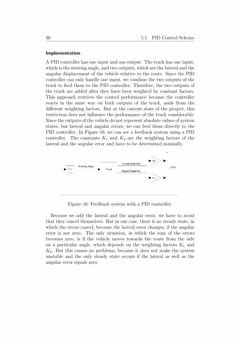
A PID controller has one input and one output. The truck has one input,which is the steering angle, and two outputs, which are the lateral and theangular displacement of the vehicle relative to the route. Since the PIDcontroller can only handle one input, we combine the two outputs of thetruck to feed them to the PID controller. Therefore, the two outputs ofthe truck are added after they have been weighted by constant factors.This approach restricts the control performance because the controllerreacts in the same way on both outputs of the truck, aside from thedifferent weighting factors. But at the current state of the project, thisrestriction does not influence the performance of the truck considerably.Since the outputs of the vehicle do not represent absolute values of systemstates, but lateral and angular errors, we can feed them directly to thePID controller. In Figure 16, we can see a feedback system using a PIDcontroller. The constants K1 and K2 are the weighting factors of thelateral and the angular error and have to be determined manually.
Figure 16: Feedback system with a PID controller.
Because we add the lateral and the angular error, we have to avoidthat they cancel themselves. But in our case, there is no steady state, inwhich the errors cancel, because the lateral error changes, if the angularerror is not zero. The only situation, in which the sum of the errorsbecomes zero, is if the vehicle moves towards the route from the sideon a particular angle, which depends on the weighting factors K1 andK2. But this causes no problems, because it does not make the systemunstable and the only steady state occurs if the lateral as well as theangular error equals zero.
37 5.2 LQR Control Scheme
5.2 LQR Control Scheme
The second approach we consider is to track the route using an LQRcontroller.
Approach
An LQR controller minimizes the cost function
J(u) =
∫ ∞
0
x(t)T Qx(t) + u(t)T Ru(t)dt (75)
by choosing an adequate control signal u(t). Q is a quadratic weightingmatrix of the system states x and R penalizes the control effort. In [5],it is shown that the cost function defined in Equation (75) is minimizedif the control signal has the form
u(t) = −Kx(t), (76)
where K is a constant matrix. According to [5], the matrix K is givenby
K = R−1BT Φ, (77)
where Φ can be determined by solving the Algebraic Ricatti Equation
ΦBR−1BT Φ− ΦA− AT Φ−Q = 0. (78)
The system matrices A and B of the lateral model of the truck werederived in Section 3.
Implementation
Since we are not able to measure all four states of the lateral model of thetruck, we have to add an observer to the control loop, which determinesthe system states based on the outputs of the truck. Figure 17 shows thecontrol loop using an LQR controller including the state observer.
A common approach to determine the system states is to simulate thedynamics of the plant in the observer. But since the silicon retina isevent based, the calculation of the integrators in the simulated plant isproblematic, because the sampling rate depends on the number of spikes,which are currently generated. Therefore, we use another approach todetermine the system states.
Since the states y and ϕz do not influence the system dynamics, we canassume that the position and the orientation of the route always equal
38 5.3 Experimental Results
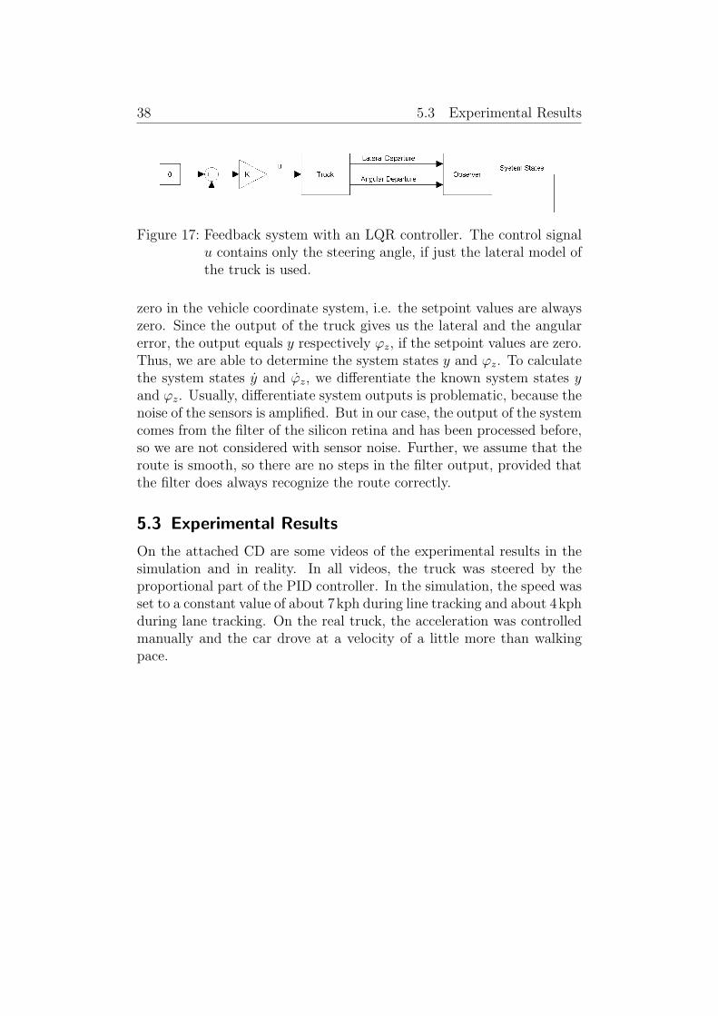
Figure 17: Feedback system with an LQR controller. The control signalu contains only the steering angle, if just the lateral model ofthe truck is used.
zero in the vehicle coordinate system, i.e. the setpoint values are alwayszero. Since the output of the truck gives us the lateral and the angularerror, the output equals y respectively ϕz, if the setpoint values are zero.Thus, we are able to determine the system states y and ϕz. To calculatethe system states y and ϕz, we differentiate the known system states yand ϕz. Usually, differentiate system outputs is problematic, because thenoise of the sensors is amplified. But in our case, the output of the systemcomes from the filter of the silicon retina and has been processed before,so we are not considered with sensor noise. Further, we assume that theroute is smooth, so there are no steps in the filter output, provided thatthe filter does always recognize the route correctly.
5.3 Experimental Results
On the attached CD are some videos of the experimental results in thesimulation and in reality. In all videos, the truck was steered by theproportional part of the PID controller. In the simulation, the speed wasset to a constant value of about 7kph during line tracking and about 4kphduring lane tracking. On the real truck, the acceleration was controlledmanually and the car drove at a velocity of a little more than walkingpace.

39
6 Conclusion
The result of this semester project is a nonlinear model of the RC monstertruck and a reduced linear model for the controller design. Further, asimulation environment in Blender has been developed, to simulate thebehavior of the truck including the silicon retina. Using this simulationenvironment, control strategies to track a route with the RC monstertruck can be tested.
Two first control strategies, a PID and an LQR controller, were im-plemented in jAER and tested in Blender as well as in reality. On thereal vehicle, some problems occurred, e.g. that the vehicle dynamics donot only depend on the velocity, but also on the battery power, and thatthere is too much noise under some terrain and light conditions, so thatthe visual filter is not able to handle all the spikes. Regarding to thecontroller design, it has to be considered that the sampling rate is notconstant, what complicates the handling of virtual integrators.
In the simulation in Blender under idealized conditions without noise,both controllers provided good results, i.e. the controllers were able totrack a line at a velocity of about 7kph and a lane at a velocity of about4kph.
On the real vehicle, the observer for the LQR controller failed becauseof the inconstant sampling rate. The best results were achieved by usingjust the proportional part of the PID controller. In this case, the truckwas able to follow a line at a little more than walking pace or to followa lane if it is pushed manually.
Future issues related to this project are to develop a method to handlethe varying sampling rate of the silicon retina robustly and to establishgood filter and control parameters, which may depend on the currentconditions. Further, considering the acceleration sensor for the controllerdesign and using cascaded control loops could improve the performanceof the control strategies.
Another future work is to install additional sensors for a more pre-cisely identification of the model parameters. At the current state of theproject, the imprecise model parameters do not yet influence the per-formance of the controller considerably, because there are other morefundamental problems to solve. But in the future when more complexcontrollers will be applied and a simulation very near to the reality isneeded, then the identification of the parameters has to be preciser.
40
Acknowledgement
I would like to thank Christian Brandli for the nice collaboration duringthis project. My thanks go also to Tobi Delbruck and Thomas Bessel-mann for the supervision and the support and to Patrick Lichtsteiner forthe construction of a new camera mount.
41 List of Figures
List of Figures
1 RC monster truck . . . . . . . . . . . . . . . . . . . . . . 32 Side view of the RC monster truck . . . . . . . . . . . . 73 Top view of the RC monster truck . . . . . . . . . . . . . 84 Side view of the body . . . . . . . . . . . . . . . . . . . . 95 Back view of the body . . . . . . . . . . . . . . . . . . . 106 Side view of a wheel . . . . . . . . . . . . . . . . . . . . 137 Suspension . . . . . . . . . . . . . . . . . . . . . . . . . . 148 Suspension forces . . . . . . . . . . . . . . . . . . . . . . 159 Top view of a wheel . . . . . . . . . . . . . . . . . . . . . 1710 Parameter identification using Matlab . . . . . . . . . . . 2711 Interaction between the simulation and the jAER package 2812 Simulation using the linearized models . . . . . . . . . . 3013 Simulation screen shot and associated spikes . . . . . . . 3214 Comparison between a recorded and a simulated output
of the silicon retina . . . . . . . . . . . . . . . . . . . . . 3415 Schematic PID controller . . . . . . . . . . . . . . . . . . 3516 Feedback system with a PID controller . . . . . . . . . . 3617 Feedback system with an LQR controller . . . . . . . . . 38
42 List of Figures
Attachments
The attached CD contains several digital files of this project. In additionto the documentation of the project, there are five folders on the CD.The content of the folders is introduced in the following.
Folder ‘jAER’
This folder contains the controller, which is called FancyDriver and im-plemented in Java.
Folder ‘Matlab’
In this folder the Matlab-files are stored, i.e. the Simulink model of thetruck and the Matlab script to linearize the model for the simulation.
The Readme-file in this folder gives more information about the han-dling of the Matlab scripts.
Folder ‘Presentation’
This folder contains the PowerPoint-presentation of our work and thevideos which were shown during the presentation.
Folder ‘Simulation’
This folder includes all files which are needed for the simulation. The sub-folder ‘Blender’ contains the Blender-file for the simulation (Truck.blend)and Blender version 2.45 for Windows, since the simulation works only inthis version. The sub-folder ‘PythonScripts’ contains the scripts, whichwere written for the simulation.
For further instructions relating to the simulation, take a look at theReadme-file, which is placed in this folder.
Folder ‘Videos’
In this folder some videos of test runs in the simulation as well as in realityare stored. In all videos, the steering angle of the truck is controlled bythe PID controller using just the proportional part. In Blender, thevelocity of the truck is set to a constant value and in the videos of thereal truck, the acceleration is controlled manually.

43 References
References
[1] http://jaer.wiki.sourceforge.net.
[2] http://siliconretina.ini.uzh.ch.
[3] http://www.blender.org.
[4] Albert Cardona. Blender’s game engine as a 3d environment simu-lator for external programs. blender conference, 2007.
[5] H. P. Geering. Regelungstechnik. Springer Berlin, 2001.
[6] L. Guzzella. Modeling and analysis of dynamic systems, 2005/2006.Lecture Notes at ETH Zurich.
[7] L. Guzzella. Analysis and Synthesis of Single-Input Single-OutputControl Systems. vdf, September 2007.
[8] The MathWorks. Matlab. http://www.mathworks.com.
[9] R. Rajamani. Vehicle Dynamics and Control. Springer, 2005.
[10] Wolfram Research. Mathematica. http://www.wolfram.com.