development of data assimilation techniques for hydrological applications€¦ · ·...

Development of Data Assimilation Techniques for Hydrological

Applications

Leila Farhadi

Department of Civil and Environmental Engineering

George Washington University

Advances in hydrological modeling

Growth in computational power

Availability of distributed hydrological Obs.

Improved understanding of physics and

dynamics of hydrologic system

Complex hydrological models

Need of concrete methods to deal with increasing uncertainty in

models and obs.

Address uncertainty:

- Understand

- quantify

- reduce

Address uncertainty

Understand

Various sources of

uncertainty:

- Model structure

- Parameters

- Initial conditions

- Observational data

Present the predictions in terms of

probability distribution

[performing probabilistic instead of

deterministic prediction/modeling]

(1) Acquisition of more informative and higher quality data

(2) Developing improved hydrological models

(better representation of physical processes and mathematical techniques)

(3) Development of techniques that can better extract and assimilate

information from the available data via model identification and prediction

Quantify

Reduce

Data Assimilation (DA) methods

Data Assimilation: Procedures that aim to produce physically consistent representations/ estimates of the dynamical behavior of a system by merging the information present in imperfect models and uncertain data in an optimal way to achieve uncertainty quantification and reduction.

Observation errors Model

Assimilation Observations

Forcing

Improved Model Results

Information on model errors

Parameter Estimation

Deterministic approaches ( calibration method)

Stochastic approaches(e.g. Generalized Likelihood Uncertainty Estimation(GLUE), Bayesian Recursive Estimation(BaRE) )

State Estimation

Kalman filtering [ e.g. Ensemble Kalman Filter]

Particle filtering(e.g. bootstrap filtering, sequential Monte carlo(SMC),…)

Variational Data Assimilation (VDA) …..

Different types of DA problems:

System(structure) Identification

Generalized likelihood uncertainty estimation (GLUE)Bayesian model averaging (BMA) ……

Simultaneous State and Parameter Estimation

-Vruget et al.[2005] Simultaneous Optimization and Data Assimilation(SODA)

- Moradkhani et al.[ 2005a,2005b] dual state-parameter estimation based on EnKF

- Joint state-parameter estimation-State augmentation [ e.g. Gelb, 1974; Drecourt et al., 2005]

Different DA problems may require different techniques/algorithms that best fit into the specific problem setting.

Assimilation of Freeze/Thaw Observations into the NASA Catchment Land Surface Model

[ Farhadi, L., Reichle, R., De Lannoy, G. J. M., Kimball, J. (2014). Assimilation of Freeze/Thaw Observations into the NASA Catchment Land Surface Model, submitted to journal of hydrometeorology]

Estimation of Land Surface Water and Energy Balance Parameters Using Conditional Sampling of Surface States

[Farhadi, L., Entekhabi, D., Salvucci, G., Sun, J. (2014). Estimation of Land Surface Water and Energy Balance Parameters Using Conditional Sampling of Surface States, Water Resources Research, 50(2), 1805-1822]

• State Estimation

• Parameter Estimation

Different DA problems may require different techniques/algorithms that best fit into

the specific problem setting.

Assimilation of Freeze/Thaw Observations into the NASA

Catchment Land Surface Model

[ Farhadi, L., Reichle, R., De Lannoy, G. J. M., Kimball, J. (2014). Assimilation of Freeze/Thaw Observations into

the NASA Catchment Land Surface Model, submitted to journal of hydrometeorology]

Estimation of Land Surface Water and Energy Balance Parameters

Using Conditional Sampling of Surface States

[Farhadi, L., Entekhabi, D., Salvucci, G., Sun, J. (2014). Estimation of Land Surface Water and Energy Balance

Parameters Using Conditional Sampling of Surface States, Water Resources Research, 50(2), 1805-1822]



The land surface (F/T) state is a critical threshold that controls

hydrological and carbon cycling and effects.

water and energy exchanges

net primary productivity

Growing season, Net Primary Productivity (NPP), Land- Atmosphere CO2 exchange patterns shift as a result of Global warming , consistent with the patterns and changes in seasonal F/T dynamics.

Thus:

Improved representation of the landscape F/T state in land surface schemes is needed.

Assimilation of F/T index should improve the simulation of carbon and hydrological processes.

Assimilation of F/T Observations into the NASA Catchment Land Surface Model

Introduction:

Figure: shows the SMMR-SSM/I daily combined AM/PM FT status for 9 April 2004. Areas colored in gray lie outside of the FT data set domain

To update the GEOS-5 land data assimilation system with a

newly designed F/T assimilation module.

To provide a framework for the assimilation of SMAP

(Soil Moisture Active Passive) F/T observations.


Objective:

the observed F/T variable is essentially a binary observation ( not continuous)

A rule based assimilation approach is proposed:


The New F/T Algorithm:

If model forecast and observation disagree on F/T variable, model prognostic

variables are adjusted to match the observed F/T more closely.

To account for model and observation errors, the delineation between frozen and

thawed regimes is defined with some uncertainty in the assimilation algorithm

F/T =f (Tsurf_nosnow, Tsnow, Tsoil)

= g( Teff ( effective temperature); asnow ( snow cover fraction) )


Teff (oC)

asnow

(%)

0

asnow_Threshold

0

100

Frozen (FT=-1)

Thawed (FT=1)

Teff=(1-α)Tsoil+ α Tsurf_nosnow

asnow : snow cover fraction(%)

asnow_threshold: depends on the microwave

frequency of backscatter/Tb.

[Higher frequency-> lower threshold and vice

versa];

F/T Detection Algorithm :

Teff

(oC)

asnow

(%)

00

100% UB_Asnow=100%

LB_Asnow

LB_Teff UB_Teff

Red region: Completely thawed

Blue region: Completely frozen

Undetermined


Observed F/T=-1 ( freeze)

F/T Analysis Algorithm :

Teff

(oC)

asnow

(%)

00

100% UB_Asnow=100%

LB_Asnow

LB_Teff UB_Teff

Teff

(oC)

asnow

(%)

00

100% UB_Asnow=100%

LB_Asnow

LB_Teff UB_Teff

Analysis happens

Teff

(oC)

asnow

(%)

00

100% UB_Asnow=100%

LB_Asnow

LB_Teff UB_Teff


Observed F/T=1 ( Thaw)

F/T Analysis Algorithm :

Teff

(oC)

asnow

(%)

00

100% UB_Asnow=100%

LB_Asnow

LB_Teff UB_Teff

Teff

(oC)

asnow

(%)

00

100% UB_Asnow=100%

LB_Asnow

LB_Teff UB_Teff

Analysis happens

Red region: Completely thawed

Blue region: Completely frozen

Undetermined

Area under investigation

45-55°N and 90-110°W

Time period :

8 year (2002-2010)

Grid:

36 km EASE grid ( 1137 grid cells)

Design Setting:


asnow Teff

asnow_threshold=10% Teff_threshold=0oC

UB_asnow=100% UB_Teff=1oC

LB_asnow=5% LB_Teff=-1oC

Experimental Setup:


Synthetic true F/T index:Produced by running the Catchment model using MERRA forcing

Synthetic observed F/T index:Produced by applying classification error (CE)* to synthetic true data set.

Open Loop ( No assimilation):Produced by running the Catchment model with GLDAS forcing.

FT Analysis ( Data Assimilation): Produced by performing FT analysis, using synthetic observation and running the

Catchment model with GLDAS forcing.

CE

MaxCE

-10 oC 0 oC 10 oC

* We assume classification error

as a function of Tsurf

Simulations:

Tsurf


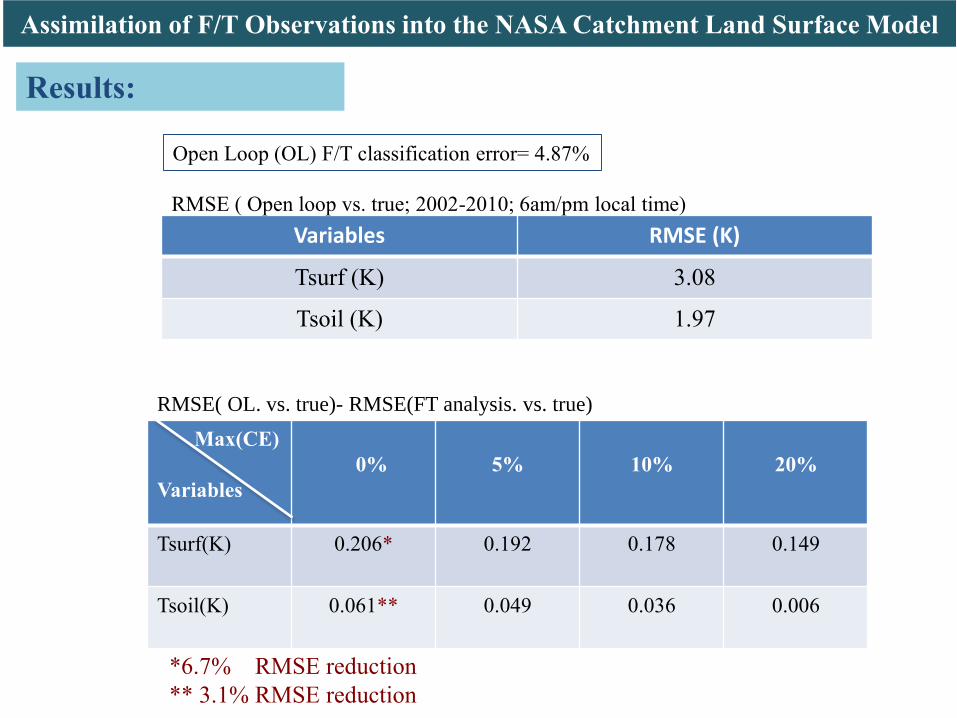
Max(CE)

Variables

0% 5% 10% 20%

Tsurf(K) 0.206* 0.192 0.178 0.149

Tsoil(K) 0.061** 0.049 0.036 0.006

Variables RMSE (K)

Tsurf (K) 3.08

Tsoil (K) 1.97

RMSE ( Open loop vs. true; 2002-2010; 6am/pm local time)

RMSE( OL. vs. true)- RMSE(FT analysis. vs. true)

*6.7% RMSE reduction

** 3.1% RMSE reduction

Results:

Open Loop (OL) F/T classification error= 4.87%


No classification error max(CE)=5% max(CE)=20%

Results:


Tsu

rf(K

) Sk

ill Im

pro

vem

en

t

Tso

il(K

) Sk

ill Im

pro

vem

en

t

α

α

Sensitivity of assimilation

results to α

Teff = (1-a)*Tsoil +a *TSurf

no-snow

Results:

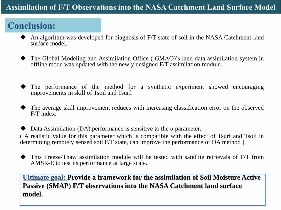
An algorithm was developed for diagnosis of F/T state of soil in the NASA Catchment landsurface model.

The Global Modeling and Assimilation Office ( GMAO)’s land data assimilation system inoffline mode was updated with the newly designed F/T assimilation module.

The performance of the method for a synthetic experiment showed encouragingimprovements in skill of Tsoil and Tsurf.

The average skill improvement reduces with increasing classification error on the observedF/T index.

Data Assimilation (DA) performance is sensitive to the α parameter.

( A realistic value for this parameter which is compatible with the effect of Tsurf and Tsoil indetermining remotely sensed soil F/T state, can improve the performance of DA method )

This Freeze/Thaw assimilation module will be tested with satellite retrievals of F/T fromAMSR-E to test its performance at large scale.


Ultimate goal: Provide a framework for the assimilation of Soil Moisture Active

Passive (SMAP) F/T observations into the NASA Catchment land surface

model.

Conclusion:

Different DA problems may require different techniques/algorithms that best fit into

the specific problem setting.

Assimilation of Freeze/Thaw Observations into the NASA

Catchment Land Surface Model

[ Farhadi, L., Reichle, R., De Lannoy, G. J. M., Kimball, J. (2014). Assimilation of Freeze/Thaw Observations into

the NASA Catchment Land Surface Model, submitted to journal of hydrometeorology]

Estimation of Land Surface Water and Energy Balance

Parameters Using Conditional Sampling of Surface States

[Farhadi, L., Entekhabi, D., Salvucci, G., Sun, J. (2014). Estimation of Land Surface Water and Energy Balance

Parameters Using Conditional Sampling of Surface States, Water Resources Research, 50(2), 1805-1822]



22

• Links (and closure) for surface water and energy balance

Surface water & energy balance

linked through latent Heat flux

The need for consistency

requires a closure function

Over bare soil this closure often can

take the form of soil moisture (s)

dependent empirical functions:

In plant continuum, it often takes

the form of :

1. Soil moisture-dependent root water extraction

resistance rg

2. Stomatal resistance rs due to plant water stressnEvaporatio Potential

nEvaporatio Actualβ(s) .1

interface atmosphere-soilat Humidity (s)h .2

Estimation of Land Surface Water and Energy Balance Parameters Using

Conditional Sampling of Surface States

Motivation:

• All Land Surface Models – LSMs include (explicitly or implicitly) a form of this closure.

• No matter how complex the closure function is, LSM’s still tend to produce an Evaporative fraction function which increases with Soil moisture or is insensitive to it

• Land response to radiative forcing and partitioning of available energy are critically dependent on the functional form (shape) of the closure relationship.

• The function affects the surface fluxes, the influence reaches through the boundary layer and manifests itself in the lower atmosphere weather

• Important as these closure functions are, they still remain essentially empirical and untested across diverse soil and vegetation conditions.

23



Motivation:

inR

24

The overarching goal of this project is to develop a scale free, calibration free technique

to better estimate the unknown parameters (e.g. the flux components) of water and energy

balance equation ( and the closure relation between the two) using discrete observation.

Estimation procedure is distinct from “calibration” since only forcing ( P, ) and state (s, Ts)

observations are used. No information about fluxes ( e.g. flux towers) is needed.

The method is scale- free, i.e. it can be applied to diverse scales of states and forcing (remote

sensing applications)

The method can be applied to diverse climates and land surface conditions using remotely

sensed measurements.



Motivation:

25

The approach is based on the conditional sampling method of Salvucci (2001) which exploits

the fact that the expected value of increments of seasonally detrended soil moisture (s)

conditioned on moisture is zero (E[ds/dt|s]=0) for stationary systems.

[Mathematical proof: conditional expectation minimizes least squared loss function]

Model parameters (sum of evaporation and drainage) are estimated by matching the soil

moisture conditional expectation of modeled fluxes to soil moisture conditional expectation of

precipitation. (E[Sum of fluxes|s]=E[P|s])

Problem in distinguishing evaporation from drainage

Result of stationarityE[ds/dt|s]=0



Methodology:

26

It can be proved that for seasonally (periodically) stationary process (Xt), The relation

E[dXt/dt|Xt]=0 holds

Result of Stationarity E[dXt/dt|Xt]=0

Soil moisture (S) and soil surface temperature(Ts) are seasonally stationary, Thus:

E[dS/dt|S]=0 and E[dTs/dt|Ts]=0

Thus by applying to the two balance equations we can separate out drainage from

evaporation( Note: both hydrologic fluxes important but not measured widely)



Methodology:

CRDETPdt

dsl

0 =

E[P | s]- E[ET | s]+ E[D | s]- E[CR | s]

0 =

E R in

¯ |Tséë

ùû- E[LE|Ts ]-E[H|Ts]-E[Pi.

pw

pw(Ts-TD ) |Ts ]-E[es Ts

4 | Ts ]

27

Example Moisture Diffusion Eq : Example Heat Diffusion Eq :

E[ds/dt|s]=0 E[dTs/dt|Ts]=0

)TT(2HLERP

2

dt

dTDs

RR

ni

s

outin

Process Unknown Par’s Form

Drainage Ks, c D(s)=Ks.sc

Capillary rise w, n CR(s)=w.sn

Thermal Inertia Pi f( soil type, soil moisture)

Neutral turbulent heat

coefficient ( CHN)α, β CHN= exp(αLAI+β)

Evaporative Fraction

( EF=LH/(LH+H))a,θs,θw EF=1-exp(-a(θ/ θs- θw/ θs)



Methodology:

S and Ts are discretized to n and m ranges respectively

0),());,0(~

);)(,0(~

21

2

2

22

1

CovN

LN

inR

P

)md.(A.)md(2

1J T

28

)(

)(

2

1

jMTRE

iMsLPE

esj

wi

in

The cost function:

d : Vector of data (n+m x1)

M: Vector of Model Counterparts (n+m x1)

A=σ-2I (n+m x n+m )

Units:W/m2

Forcing uncertainty:

Note: Estimation procedure is distinct from “ calibration” since only forcing data ( P, )

and state observation (s, Ts) are used. No information on fluxes ( e.g. Problematic evaporation

and drainage) is needed.

Where:

n] w,c, ,K,P,C a,,,[:parametersUnknown

siHNws

,....|,|,.....,LPE:

2121 sins TRETREsLPEs in

d

inR



Methodology:

- Minimize nonlinear Cost Function J

- Estimation of Uncertainty Bounds

Inverse of Hessian of Cost function is an approximation for the Covariance matrix.

Covariance matrix is used to estimate the uncertainty of any model output and thus determine which aspects of the model are poorly determined by the data

First Order Second Moment propagation of uncertainty ( FOSM) analysis, or Monte Carlo method is used to define the uncertainty around different flux components.

29



Methodology:

Determining the sufficiency of a particular data set to determine the model parameters

1- Uncertainty of each individual parameter should be reasonable in physical sense.

2-Uncertainty of the least well-determined combination of variables given by the eigenvectors of Hessian

should be reasonable.

3- Correlation matrix between unknown variables should be reasonable.

30

-Linear dependency between variables is a sign of discrepancy

between data and model

-Best scenario: The correlation between all the parameters is small,

-The next best scenario: High correlation is only between parameters representing

one flux type and suggests the model is robust with regard to flux components

-The worse scenario: The correlation between parameters representing different flux

types is high and/ or physically not meaningful.



Methodology:

• 30 year of hourly meteorological data for humid climate of Charlotte North Carolina obtained from “ Solar and Meteorological Surface Observational Network” (SAMSON) [National Climate Data Center];

• Simultaneous Heat and Water( SHAW) model was used to derive consistent hourly time series of state and fluxes

• Assume 20% precipitation and radiation error.

• 8 unknown parameters a = Ks,c,w,n,CHN ,a,Sw,qs[ ]



Synthetic test

2- Optimization with 8 unknown variables

swHNs θSa CnwcK ,,,,,,,

32

Data is insufficient to determine the model states with acceptable accuracy- linear dependency is generated as seen in the

correlation matrix

w~0; its variation is high;

in addition, n is large, Sn is very small ( 0<S<1)

Thus, WSn is negligible

Due to high linearity btw “ Ks ,θs” and “ a, θs”

Taking θs out of the parameter space will improve

the condition number of Hessian ;

( replace : θs ~ max( recorded θ) )

This is not a sample correlation but derived from

Hessian and related to shape of J around minimum.

Used for diagnosing collinearity and has no

statistical significance.



Synthetic test

wHNs SaCCK ,,,,

33

-Parameters are estimated reasonably well

-High correlation between Ks and C is the sign of robust estimation of Drainage.

Ks increases Ks.Sc increases

C increases Ks.Sc Decreases

-“CHN and a” parameters have negative Correlation;

Increase in parameter “CHN” Increase in estimated sensible heat flux

Decrease in parameter “ a” Decrease in estimated Latent heat flux

This result is physically meaningful, since the sum of sensible heat flux( H) and Latent

heat flux (LE) represent the available energy to the system ( Rn-G) and when the

available energy to the system is constant, an increase in H results in a decrease in LE

and vice versa.



Synthetic test

34

Comparing Actual EF and model estimate of EFComparing Actual /measured net soil water flux and its

model counterpart

× 1000.4 0.5 0.6 0.7 0.8 0.9 10

0.2

0.4

0.6

0.8

1

1.2

SM(%)

EF=

LE/L

E+H

Actual/Measured

Estimate

Estimate(+/-)err

0.4 0.5 0.6 0.7 0.8 0.9 1-20

-10

0

10

20

30

40

50

SM(%)

Soi

l net

Dra

inag

e(m

m/d

ay)

Actual/Measured

Estimate

Estimate(+/-)err

× 100

The closure function EF(s)=LE/LE+H is well estimated in this synthetic data set

This approach is robust at point scale



Synthetic test

3 Field sites were investigated:

Vaira Ranch, grassland, CA, Mediteranation climate

Audubon Research ranch, grassland, AZ, Arid/semi arid climate

Santa Rita Mesquite , woody savanna, AZ, Arid/semi arid climate

35



Field site test

Source of Data ( estimation and validation)

- AMERIFLUX ( Tower data)

Soil water content θ ; Wind speed( u), Air temperature (Ta), Soil surface Temperature (Ts),

Precipitation ( P), Net radiation (Rn)

- MODIS ( Satellite data)

LAI

Error of data

εE[ P|s]~ N(0, (6% E[ P|S])2); εE[ Rin|s]~ N(0, (8% E[ Rin|Ts])2);

36



Field site test

37

Vaira Ranch, grassland, CA

EF=LE/L

E+H

SM(%) ×100

CHN

LAI

Daily e

stim

ate

d H

(W

/m2)

Measured H (W/m2)

Daily e

stim

ate

d L

E (W

/m2)

Measured LE (W/m2)

SM(%)×100

Dra

inage

(mm/d

ay)

30 published validations of remote sensing based estimated flux against ground based measurements of evapotranspiration

shows an average RMSE value of about 50 W/m2 (Kalma et al., 2008).



Field site test

38



Field site test

• Distinct Closure function

The Gourma meso scale site in Mali of West Africa is an area located in the Gourma region. (14.5-17.5 ON, 1-2 OW), 40,000 km2 area.

Why this region

1- vast spatial and temporal coverage, remote sensing data which give access to surface variables in this area;

2- Gourma region is located in Sahara & Sahelian-Sahara climate; Evaporation is generally water limited ( EF=EF(S)) ;

3- Runoff can be considered negligible in most areas; 39

Reference [ AMMA Documentation]



Remote sensing

Var Definition Source of Data Spatial

Resolution

Temporal

Resolution

u Wind speed AMMA-ECMWF 50km 6hr

Ta Air Temp AMMA-ECMWF 50km 6hr

Rs Down Welling short wave SEVIRI 3km 15 min

α albedo SEVIRI 3km Daily

LAI Leaf Area Index SEVIRI 3km Daily

P Precipitation PERSIANN 4km hrly , daily

S Soil Moisture AMSR-E 25km 1:30 pm;1:30 am

Ts Surface Temperature SEVIRI 3km 15 min

TD Soil Deep Temperature Filtering Ts 3km 15 min

40

- 2008 data sets were selected.

- Data were aggregated to present daily time step

- Data are interpolated on a 3km*3km grid



• In order to reduce dimensionality, USGS categorical soil maps are used to find common soil hydraulic

parameters in similar regions ( alternative dimensionality reduction approaches can be applied)

41

Sand

Loamy Sand

Clay

Loam ----

Clay

Loam

Loamy Sand

Sand



Sand region….

Sand pixels ~ 81% of the pixels corresponding to the 4 different soil categories)

),,,, ws SaK

42

Parameters are estimated robustly

Correlation btwn different parameters

is reasonable & physically meaningful



Validating The results ….

Agoufa flux tower site

hourly H, LE, LE/(LE+H)

• Soil type: Sand

• Vegetation type: Grassland

• Soil water content: AMSR-E data interpolation

43

0 0.2 0.4 0.6 0.8 10

0.1

0.2

0.3

0.4

0.5

0.6

0.7

0.8

0.9

1

EF=LE/L

E+H

SM(%)×100

Daily E

stim

ate

d H

(W/m

2)

Measured H(W/m2)

0 100 200 300 400 500 6000

100

200

300

400

500

600

r=0.56

RMSE=81.8W/m2



Validating the results …

Map of water balance residual (runoff/runon) over the Gourma region

-2 -1.8 -1.6 -1.4 -1.2

15

15.5

16

16.5

17

Longitude

Latitu

de

Runoff(+)

(mm/day)

0.2

0.4

0.6

0.8

1

1.2

1.4

1.6

1.8

-2 -1.8 -1.6 -1.4 -1.2

15

15.5

16

16.5

17

Longitude

Latitu

de

Standard Error

(mm/day)

0.15

0.2

0.25

0.3

0.35

0.4

0.45

0.5

0.55

0.6

0.65

-2 -1.8 -1.6 -1.4 -1.2

15

15.5

16

16.5

17

Longitude

Latitu

de

Runon(-)(mm/day)

-2.2

-2

-1.8

-1.6

-1.4

-1.2

-1

-0.8

-0.6

-0.4

-0.2

-2 -1.8 -1.6 -1.4 -1.2

15

15.5

16

16.5

17

Longitude

Latitu

de

Standard Error (mm/day)

0.2

0.3

0.4

0.5

0.6

0.7

0.8

0.9

Yearly average water balance equation over all the pixels results in the map of runoff/ runon (+/-)

The errors in this estimation methodology manifests itself in the form of runoff/ run residuals

The map of runoff/ runon corresponds well with the characteristics of Gourma region

Runoff (+) (mm/day) Runon (-) (mm/day)Standard error (mm/day) Standard error (mm/day)

Latitu

de

Latitu

de

Latitu

de

Latitu

de

Longitude Longitude Longitude Longitude



45

0 0.2 0.4 0.6 0.8 10

0.1

0.2

0.3

0.4

0.5

0.6

0.7

0.8

0.9

1

SM(cm3/cm

3)

EF

sand

Loamy sand

Loam

clay

Soil water potential increases between coarser to

finer soils.

Higher water potential is a barrier to water

extraction, thus the rate of Evaporation from soils

with coarser texture is higher than from soils with

finer texture.

Validating the results …

EF-SM relationship for different soils

SM(%) x100



46

Day 190

Day 191

Day 192

Evaluating the results …

Precipitation- Evaporation patterns

-2 -1.6 -1.2

15

15.5

16

16.5

17

Longitude

La

titu

de

Precip(mm/day)

0 50

-2 -1.6 -1.2

15

15.5

16

16.5

17

Longitude

La

titu

de

ET(mm/day)

0 5 10

-2 -1.6 -1.2

15

15.5

16

16.5

17

Longitude

La

titu

de

SM (cm3/cm

3)

0 0.5 1

-2 -1.6 -1.2

15

15.5

16

16.5

17

Longitude

La

titu

de

Precip(mm/day)

0 50

-2 -1.6 -1.2

15

15.5

16

16.5

17

LongitudeL

ati

tud

e

ET(mm/day)

0 5 10

-2 -1.6 -1.2

15

15.5

16

16.5

17

Longitude

La

titu

de

SM(cm3/cm

3)

0 0.5 1

-2 -1.6 -1.2

15

15.5

16

16.5

17

LongitudeL

ati

tud

e

Precip(mm/day)

0 50

-2 -1.6 -1.2

15

15.5

16

16.5

17

Longitude

La

titu

de

ET(mm/day)

0 5 10

-2 -1.6 -1.2

15

15.5

16

16.5

17

Longitude

La

titu

de

SM(cm3/cm

3)

0 0.5 1

Note: No water balance or soil moisture

accounting used

SM(%)

SM(%)

SM(%)



Methodology developed to use both water and energy balance to constrain parameter estimation of surface energy and water balance

Method is distinct from traditional calibration because it does not need flux information ( eg. problomatic drainage and evaporation data) to estimate parameters

Only forcing (P, ) and states (s,Ts) used; hence scalable for remote sensing and mapping applications

Feasibility demonstrated at point-scale with synthetic data (true parameters known for evaluation) and Ameriflux field site data

Application over West Africa using remote sensing shows feasibility of using satellite data to estimate effective values of important land surface model parameters

inR

47



Conclusion:

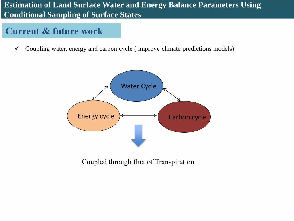
Coupling water, energy and carbon cycle ( improve climate predictions models)

Energy cycle Carbon cycle

Water Cycle

Coupled through flux of Transpiration

Current & future work



Thank you for your attention

development of data assimilation techniques for hydrological applications€¦ · ·...

Documents