Development of a Low Cost Ligation-based SNP

Genotyping Assay to Trace Maternal Ancestry in

Mitochondrial DNA

A thesis submitted by

Kaitlin Minnehan

In partial fulfillment of the requirements for the degree of

Bachelor of Science with Honors

in

Chemistry

TUFTS UNIVERSITY

May 2010

Advisor: Professor David R. Walt

ii

Acknowledgments

I would like to thank my thesis advisor, Dr. David R. Walt, for his

guidance throughout my two years of research. He gave me the opportunity to

participate in a project that has challenged me and helped me grow as a scientist

and an individual. I would like to thank Dr. Joshua Kritzer and Dr. Christopher

LaFratta for serving on my thesis committee. Dr. LaFratta’s insights and

assistance during my research has been invaluable.

To Aaron Phillips and Dr. Ryan Hayman, I thank you for your constant

patience and encouragement from day one. Without the two of you, this project

would not have been possible and for that I am truly grateful. I would like to

thank my lab partner and friend, Sarah Philips for her knowledge and support

throughout this project. A thank you goes to all the post docs, graduate students,

and undergraduate students in the Walt lab for their insights into my research: Dr.

Dimitra Toubanaki, Cary Lipovsky, Varandt Khodoverdian, Saumini Shah,

Shrikar Rajogopal, and to our Project Coordinator, Meridith Knight.

Finally, I would like to thank my family and friends, without them I would

not be where I am today. Mom, Dad, and Bret, thank you for your loving support

and guidance. Jesslyn, Cara, Whitney, and Fanna, thank you for your constant

encouragement each and every day.

iii

Abstract

A high-throughput single nucleotide polymorphism (SNP) genotyping

assay based on the Illumina GoldenGate platform was developed to study

mutations associated with human migration in mitochondrial DNA (mtDNA)

isolated from 150 saliva samples. Populations with similar migratory routes,

commonly known as haplogroups, have specific positions of mtDNA mutations

that are highly correlated and maternally inherited. An extensive literature search

was performed to identify potential SNPs of interest. From the data obtained, a

list of working SNPs was used to develop a low cost ligation-based genotyping

assay that can be performed with minimal equipment and experience. The assay

utilizes allele-specific probes (ASPs), which are complementary to either the

mutant or normal base for each SNP, and locus-specific oligonucleotide probes

(LSPs) that anneal to the region immediately flanking a target SNP. Ligation of

the biotinylated ASP to the poly dA-tailed LSP is highly specific and dependent

on the SNP site’s identity. The signal is then amplified through thermally cycled

denaturing, annealing, and ligating to create many products from each target

strand. The ligation products are then deposited onto a lateral flow biosensor

(LFB). Ligated strands are captured by streptavidin, allowing for a fast,

colorimetric readout with poly dT-functionalized nanospheres. Over 40 SNPs

have been successfully investigated using the low cost ligation assay and can now

be used in a classroom to teach students about genetics and DNA analyses while

learning about their ancestor’s migratory history.

iv

Table of Contents

Acknowledgments ii

Abstract iii

Table of Contents iv

Part I. Introduction

1. Background on Howard Hughes Medical Institute Research Project 2

2. Maternal Ancestry and Mitochondrial DNA 2

3. Human Migration Patterns 6

4. Phylotree and Its Construction 8

5. Introduction to SNP Genotyping Methods 11

5.1. Enzyme Mismatch Cleavage 12

5.2. Single Base Extension 14

5.3. Oligonucleotide Ligation Reaction 15

6. Motivation for Creating an Inexpensive SNP Genotyping Assay 18

Part II. Illumina GoldenGate Genotyping Assay

1. Introduction 22

2. General Workflow and Protocol 22

3. BeadStudio Analysis 26

4. Designing an OPA 27

4.1. Problems with OPA I 29

4.2. Improvements to OPA II 30

5. Custom Phylotree 31

6. Final SNP Calls from GoldenGate Analysis 32

Part III. Creating a Bench Top Genotyping Assay

1. DNA Purification 35

2. Amplex Red and Quanta Red Enzymatic Readout 37

3. Solid Substrates 49

v

3.1. V-Arrays 49

3.2. Lego Arrays 52

3.3. Lateral Flow Biosensors 54

3.4. Making Beads 59

4. Enzymatic Assays Researched 71

4.1. Enzymatic Cleavage 71

4.2. Single Base Extension 80

5. Ligation 90

Part IV. Conclusions and Future Work 111

Appendix

A.1. Illumina GoldenGate Assay Probe Sequences 114

A.2. Illumina GoldenGate SNP Calls 116

A.3. PCR Primers and Ligation Probes 122

A.4. Working SNPs 125

A.5. Oragene DNA Purification Protocol 127

A.6. EDC Coupling Protocol 128

A.7. Poly-dA Tailing Protocol 130

A.8. Biosensor Creation Protocol 131

A.9. PCR Protocol 135

A.10. Ligation Reaction and Readout Protocol 137

Part I. Introduction

2

1. Background on Howard Hughes Medical Institute Research Project

The Howard Hughes Medical Institute (HHMI), a non-profit biomedical

research organization, grants money to institutions looking to promote the

advancement of scientific education in undergraduate and high school classrooms.

Professor Walt received an HHMI Professor’s Award in 2006, with the idea of

creating laboratory experiments that would introduce the modern biotechnology

and analytical methods developed in his research group to younger students. The

grant provided funding for myself and my fellow undergraduate researchers the

opportunity to experience aspects of individual research, while being overseen

and working alongside graduate student and post doctoral mentors.

In this multi-faceted, multi-year project, the primary task was to create a

low-cost assay to trace maternal ancestry. The project focused on single

nucleotide polymorphism (SNP) genotyping of mitochondrial DNA (mtDNA), to

identify the origins of an individual’s ancestors. The work detailed in this thesis

demonstrates an experiment that will be useful in teaching the basics of DNA

analysis, genetics, and basic laboratory skills, while allowing students to discover

personal information about their ancestor’s history.

2. Maternal Ancestry and Mitochondrial DNA

Genomic DNA is present in the nucleus of cells and is passed down

equally from both parents, whereas mitochondrial DNA is solely passed down

maternally.1 Without any recombination occurring between mtDNA, the genetic

material is a useful tool for tracing information along ones maternal side.

3

Mitochondrial DNA exists as a closed circular loop of duplex DNA nearly 16,600

base pairs in length2 and is derived from the circular DNA of bacteria, engulfed

by ancestors of our eukaryotic cells.3 A single cell has been found to contain

1,000-10,000 molecules of DNA, contributing to the high yield of mtDNA after

isolation.4

The mitochondrial genome has been found to mutate 5-10 times faster

than nuclear DNA.5 A mutation, called a single nucleotide polymorphism (SNP),

is a single nucleotide in a DNA sequence that differs between members of a

species and can provide important information about an individual. With so

many SNPs present in the small region of ~16.6 kb, it has become very difficult to

identify specific mutations in the mitochondrial genome. When designing PCR

primers and genotyping probes, the sequence surrounding the SNP of interest may

contain other SNPs, resulting in inefficient hybridization of probes and primers

utilized in sequencing.

The analyses of mtDNA sequences can be used to trace maternal ancestry

back hundreds of thousands of years. The relationship between two individuals

can be determined by comparing the variations between the two genomes and the

percentage of overlap seen within the sequences.6 A comparison between the

SNPs of a population can be used to determine maternal lineage. Conventionally,

the comparison is made between a sample and the revised Cambridge Reference

Sequence (rCRS), which is the mitochondrial genome of one individual of

European descent that was sequenced for use as a reference point.7 With this

standard reference, any difference in a compared sequence is considered a

4

mutation. As our ancestors traveled throughout the world, settling in different

communities and reproducing with others in the same population, their mtDNA

evolved with similar mutations, allowing SNPs found in today’s individuals to be

used to trace an individual’s ancestry back hundreds of thousands of years.

Some of the first research done with human mtDNA to identify and

categorize SNPs used restriction enzymes to digest the entire genome. Brown’s

study isolated DNA from 21 individuals with diverse geographic backgrounds and

identified differences in mtDNA using restriction-enzyme fragment length

polymorphism (RFLP).8 After hundreds of studies were done to find correlations

between different SNPs and geographic regions, he was able to find relationships

between individuals from similar backgrounds and the patterns of SNPs.

Eventually, portions of the mitochondrial genome were sequenced to find

more comprehensive information. Initial tests were run looking at mutations for

medical conditions including Parkinson’s disease, mitochondrial myopathy, and

cardiomyopathy in Japanese populations.9,10

Studies within this population were

further explored to analyze the phylogenetic relationships between individuals in

Eastern Asia.11

With complete sequencing available, others started to look at the

original migration out of Africa to develop a detailed route, giving more

information to migration patterns.12

While complete mitochondrial genomes were

being sequenced, attention was drawn to the inconsistent mutation rate along the

genome. It was found that the control region, including the hypervariable

segments HVS-I and HVS-II, evolved more rapidly than the coding regions.13

Although the high mutation rate made it difficult to find patterns among

5

individuals, it also contributed to the dense amount of information that could be

obtained within the region. Complete sequences of the control region provided

information necessary to establish concrete migration patterns.14

While the

introduction of sequencing contributed greatly to phylogenetic networking, it is

expensive and time consuming.

A new method of minisequencing was introduced that shortened the time

of sequencing by focusing on small portions of the mitochondrial genome. The

Affymetrix MitoChip (Santa Clara, CA) is a directed array that uses thousands of

known probes to sequence portions of the mitochondrial genome.15

The array has

been used to genotype hundreds of individuals and diagnose many diseases,

including Alzheimers,16

breast cancer,17

pancreatic cancer,18

hearing loss,19

head

and neck cancer, 20,21

and gastrointestinal cancer.22

Photolithography is used to synthesize oligonucleotides on the surface of

the Mitochip. A photomask is used to add one protected nucleotide at a time to

the surface. After several (sometimes up to a hundred) photomasks have been

used to add single nucleotides to known locations, the array consists of thousands

of known sequences in known locations.23,24

By constructing an array with

thousands of probes complementary to portions of the mitochondrial genome,

minisequencing allows for a faster readout than complete genome sequencing.

While the MitoChip and minisequencing have improved the time, it is still

extremely costly. Through previous timely and costly work, we now have

sequences that can be used to develop faster and cheaper methods by looking

6

directly at known locations. Genotyping looks specifically at known SNPs

instead of obtaining excess information about surrounding sequences.

3. Human migration patterns

Human migration patterns are determined by studying the patterns of

SNPs in a population. A population consisting of similar SNPs is recognized as a

single haplogroup, which is used to categorize individuals based on geographic

location and migration patterns. By categorizing an individual into a haplogroup,

it is possible to trace migration routes by observing the branching points of all

associated haplogroups. Larger main haplogroups break down into smaller, more

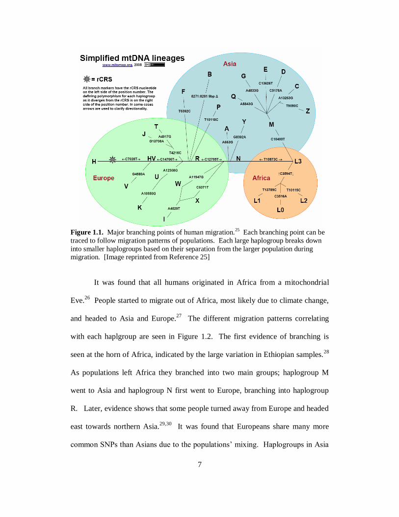
specific haplgroups, in a tree formation as seen in Figure 1.1. Therefore, if an

individual indentifies for a small sub-haplgroup, they are in every larger

haplgroup higher on the tree.

7

Figure 1.1. Major branching points of human migration.

25 Each branching point can be

traced to follow migration patterns of populations. Each large haplogroup breaks down

into smaller haplogroups based on their separation from the larger population during migration. [Image reprinted from Reference 25]

It was found that all humans originated in Africa from a mitochondrial

Eve.26

People started to migrate out of Africa, most likely due to climate change,

and headed to Asia and Europe.27

The different migration patterns correlating

with each haplgroup are seen in Figure 1.2. The first evidence of branching is

seen at the horn of Africa, indicated by the large variation in Ethiopian samples.28

As populations left Africa they branched into two main groups; haplogroup M

went to Asia and haplogroup N first went to Europe, branching into haplogroup

R. Later, evidence shows that some people turned away from Europe and headed

east towards northern Asia.29,30

It was found that Europeans share many more

common SNPs than Asians due to the populations’ mixing. Haplogroups in Asia

8

have much more variation because populations settled in a particular region and

did not mix with any other settlements. These routes have been researched

extensively and compiled in Torroni’s review.31

Figure 1.2. Migration routes of human beings dating back to 170,000 years ago.

25 All

humans originated in Africa and migrated out, branching into the two main out of Africa haplogroups, M and N. Individuals in haplogroup M headed west to Asia and later to the

Americas, while haplogroup N moved into Europe. [Image reprinted from Reference 25]

4. Phylotree and its Construction

Thousands of human genomes have been sequenced and used to find

patterns of similar SNPs within populations. Many studies have been completed

focusing on small populations around the world to find phylogenetic relationships

between the inhabitants. However, inconsistencies have been found when

comparing studies. Each independent study focused on a specific population, but

many new haplogroups and branching points have recently been introduced,

making it difficult to follow the relationships between different haplogroups. A

9

recent paper by van Oven and Kayser compiled from approximately 100 studies

to construct an up-to-date universal phylotree that could be used by everyone.32

Previous research on this project in our lab was based on the work done by

Herrnstadt, who focused on establishing phylogenetic networks within a

geographic region.33

While many of these same SNPs are still being investigated,

several of the branching points noted in the paper have been restructured.

Therefore, our lab’s previous work placed individuals into the correct haplogroup,

however the relationships between the haplogroups were not correct. Van Oven

worked to find consistencies among almost 100 papers in order to create the

universal tree. The original nomenclature proposed by Richards34

introduced

many inconsistencies among other studies. In some instances the same name was

used for different haplogroups,35,36,37

and in other situations different names were

used for the same haplogroup.38,39,40

Van Oven created a complete phylotree that

is available at phylotree.org and is updated with current information in order to

maintain a tree that can be used to keep studies consistent. A small portion of the

website is seen in Figure 1.3 showing the branching points off of the main

haplogroup U. The position number of each SNP is seen along with references

for the SNP identity and location.

10

Figure 1.3. Snapshot from phylotree.org. The main haplogroup U, branches into small

more detailed haplogroups. Each SNP that identifies a haplogroup is listed by position

with coding region mutation (577-16023) in black and control region mutations (16024-576) in blue. The reference where each SNP was found is shown to the right of each

SNP. [Image reproduced from phylotree.org]

A simplified version of the tree is seen in Figure 1.4, to show major

branching points that can be compared to the original tree made by MitoMap in

section I.3.

Figure 1.4. Simplified version of the phylotree showing major branching points and

haplogroups. The original haplogroup out of Africa is L3 which breaks down into N, leading to Europe and M, heading west to Asia. [Image reproduced from reference 32]

11

5. Introduction to SNP Genotyping Methods

Analysis of different individual’s DNA sequences has revealed positions

in which one of two different bases could be present. These SNPs occur when a

single base mutates to a new base and is passed down through generations,

making it possible to trace mutations through family members. Millions of SNPs

have already been identified and can each encode for many different

characteristics. Exploring different genotyping methods has increased the ability

to genotype larger populations and lowered the cost of genotyping.

The invention of the polymerase chain reaction (PCR) was the necessary

first step in creating SNP genotyping assays (Figure 1.5). The task of identifying

a single base in 6 billion bases of genomic DNA and ~16.6 kilobases of mtDNA

is extremely difficult without shortening the sequence to a more manageable size.

PCR uses two synthetic primers complementary to the target DNA. Each primer

binds to one of the two strands of dehybridized target DNA surrounding the

desired region, and a DNA polymerase is introduced along with the all four

deoxyribonucleotide triphosphates (dNTPs). The polymerase adds each dNTP to

the end of the hybridized primer in order to extend the sequence creating a

complement to the target strand.41

PCR is important because as long as the

flanking regions are known, the polymerase will add the dNTPs specific to the

target strand, incorporating any mutations present. After the reaction runs

through many cycles of dyhybridization, annealing and extension, the final

product consists of a concentrated solution of billions of copies of DNA of a

specified length as determined by the location of the hybridized primers. PCR has

12

enabled researchers to work with high concentrations of short DNA in order to

maximize specificity in a concentrated sample.

Figure 1.5. PCR starts with the dehybridization of the long target strand. Primers anneal

to the 5’ end of the target and extend to the 3’ end with the addition of dNTPs and

polymerase. After dehybridization, the number of strands doubles to four. Primer annealing and extension takes place again, resulting in 8 strands, then 16. After 30 cycles

there are billions of copies of the desired region.

5.1 Enzyme Mismatch Cleavage

Nucleases are enzymes that naturally cleave the phosphodiester bond

between nucleotides. Researchers have used this class of enzymes for mismatch

detection in duplex DNA.42

Original nucleases that were isolated for mismatch

detection include the T4 endonuclease VII and mung bean endonuclease. The

13

specific nucleases found were able to detect a single mismatch at a SNP site and

cleave the double stranded DNA.43

Probes can be designed complementary to a

particular base, and the regions flanking the base, so when a non-complementary

base is present, the mismatch is detected and cleaved on the 3’-end of each strand

as seen in Figure 1.6. The cleavage products can then be analyzed using gel

electrophoresis or Southern blots.42,44

A more recent discovery of the CEL 1

endonuclease from celery, has demonstrated increased cleavage specificity.45

While other enzyme’s reaction conditions include a pH below 7 and increased

temperatures of 60 °C, the optimum conditions of CEL 1 has a pH between 7 and

8 and temperatures between 37-40 °C, allowing for more moderate reaction

conditions.44

Changing the reaction conditions to an environment more

compatible with DNA allowed for increased cleavage specificity, where CEL I

has demonstrated useful in the detection of a single mutation.46

Figure 1.6. A probe is designed to surround the SNP position. If there is a mismatch, the endonuclease will detect the mismatched bases and cleave the double stranded DNA

at the 3’ end of the mismatch. The cleavage is then detected using gel electrophoresis or

Southern Blots.

14

5.2 Single Base Extension

Single Base Extension analyzes a single base in the genome using a

polymerase and dideoxyribonucleotide triphosphates (ddNTPs). Oligonucleotides

are designed to be complementary to the target sequence and end before the SNP

at the 3’ end.47

Polymerase and ddNTPs are then added to be incorporated into

the sequence. The polymerase adds the ddNTP to 3’-end of the probe,

complementary to the SNP base. Only the ddNTP complementary to the expected

base is labeled, therefore when the ddNTP is detected after the reaction is

complete, the base will be known as seen in Figure 1.7.48

Single base extension

incorporates ddNTPs to prevent extension after the addition of one base, as

ddNTPs lack the 3’-hydroxyl group on their sugar, therefore no additional

nucleotides can be incorporated because the phosphodiester bond cannot be

created between the 5’-phosphate and 3’-carbon.49

Many different detection methods have been explored to be used with

primer extension. Only the ddNTP complementary to the SNP base contains a

label, therefore if a different base was present at the SNP site, the lack of signal

indicates that the allele is not present. Originally, radioisotopes where used to

identify the SNP base. The complemenetary ddNTP could be labeled with either

a radioisotope of phosphorous46,50

or hydrogen47

and could easily be detected.

Later, fluorescenctly labeled ddNTPs were introduced allowing for higher

throughput.51

Instead of adding only one labeled ddNTP, all four ddNTPs could

be added, each with a different fluorescent label, and could be detected using the

different excitation and emission wavelengths of each label. Colorimetric

15

readouts have also allowed for the easy SNP detection.52

The principles

introduced by primer extension can be expanded upon in order to detect SNP

using different immobilization techniques and detection methods.

Figure 1.7. Single base extension is used to identify a specific SNP. A capture probe is

designed to anneal to the target strand 3’ to the SNP and end before the SNP. A. A

complementary fluorescent ddNTP is added to the mixture and the presence of signal indicates the SNP is present . B. An unmodified ddNTP can be added to test for the

other allele and the absence of a signal shows the other allele is present.

5.3 Oligonucleotide Ligation Reaction

The Oligonucleotide Ligation Reaction (OLR) uses a DNA ligase to form

a phosphodiester bond between two adjacent probes hybridized to a target strand.

The ligase requires complete hybridization of both probes to the target in order to

catalyze the formation of the bond.53

For SNP genotyping, two probes are

introduced into solution: the Locus-Specific Oligonucleotide (LSO), which stops

16

before the SNP and the Allele-Specific Oligonucleotide (ASO), which includes

the base complementary to the SNP. Therefore, if the SNP is not present, the last

base of the ASO will not anneal, creating a tail and the ligase will not form a bond

(Figure 4A). However, if the SNP is present, the ASO will hybridize completely,

and the ligase will form a phosphodiester bond with the LSO (Figure 1.8). The

LSO and ASO can be modified in order to create a read-out. Often one

modification is used to immobilize the newly formed strand to a surface and one

modification is used for a readout.52

Different readouts have been explored that

included radioactivity, fluorescence and color absorption.

The catalysis of the formation of the phosphodiester bond between directly

adjacent 3’-hydroxyl and 5’-phosphoryl termini is done in three steps involving

two intermediates.54

First the ligase reacts with either ATP or NAD to form

ligase-adenylatae. Next the adenylel group is transferred to the DNA to form a

bond between the 5’-phosphoryl terminus and AMP, while PPi is released. Last,

the 3’ hydroxyl group attacks the 5’-phosphate to form the phosphodiester bond

and the AMP leaves.53

17

Figure 1.8. A locus-specific probe binds 3’ to the SNP and an allele-specific probe binds

5’ to the SNP and includes the complementary base of the SNP. One probe contains a signal molecule and the other contains a substrate for immobilization. A. When the ASP

diagnostic base is complementary to the SNP, ligation occurs between the ASP and LSP.

If the ASP diagnostic base is not complementary to the SNP, there is a tail and no ligation occurs resulting in three separate strands of DNA after dehybridization.

The read-out of the ligation reaction can be enhanced by amplifying the

signal. The ligation amplification reaction (LAR) provides a means of producing

many signal molecules from a single target strand.55

The reaction still requires

the dehybridization of target DNA followed by the hybridization of the ASO and

LSO and ligation, however the reaction is cycled over and over to increase the

signal. By adding excess ligation probes, several ligation reactions can occur

using a single target strand with multiple probes. The discovery of thermostable

ligase56

has allowed for easy cycling similar to PCR, using a thermocycler that

alternates between a dehybridization temperature and an annealing and ligation

temperature. By adding a read-out method to the ligation probes, the signal is

significantly amplified.

18

6. Motivation for Creating an Inexpensive SNP Genotyping Assay

Using of the Illumina GoldenGate Genotyping assay, we investigated the

success of our custom sequences in order to identify single mismatches in the

mitochondrial genome. After testing over 100 samples, we generated a database

of the sample’s known SNP calls and haplogroups that could be used later. The

GoldenGate assay provided very precise results, however it was still costly and

time consuming. By modifying the GoldenGate sequences in conjunction with

the information obtained from the standard samples, a low cost ligation assay was

developed. The ligation assay used basic laboratory equipment to produce a

colorimetric readout on a nitrocellulose biosensor within hours. By utilizing basic

laboratory skills and equipment, the assay could be easily adapted for use in high

school and undergraduate classrooms.

1 Giles, R. E.; Blanc, H.; Cann, H. M.; Wallace, D. C. Proc. Natl. Acad. Sci. USA

1980, 77, 6715-6719. 2 Brown, W. M.; Vinogra, J. Proc. Natl. Acad. Sci. USA 1974, 71, 4617-4621.

3 Margulis, L. Symbiosis in Cell Evolution (Freeman, San Francisco, 1981)

4 Bogenhagen, D.; Clayton, D. A. J. Biol. Chem. 1974, 249, 7991-7995.

5 Brown, W. M.; George, J. J.; Wilson, A. C. Proc. Natl. Acad. Sci. USA 1979, 76,

1967-1971. 6 Potter, S. S.; Newbold, J. E.; Hutchison, C. A. I.; Edgell, M. H. Proc. Natl.

Acad. Sci. USA 1975, 72, 4496-4500. 7 Anderson, S.; Bankier, A. T.; Barrel, B. G.; de Bruijn, M. H. L.; Coulson, A. R.;

Drouin, J.; Eperon, I. C.; Nierlich, D. P.; Roe, B. A.; Sanger, F.; Schreier, P. H.;

Smith, A. J. H.; Staden, R.; Young, I. G. Nature 1981, 290, 457-465. 8 Brown, W. M. Proc. Natl. Acad. Sci. USAo 1980, 77, 3605-3609.

9 Ozawa T. et al Biochem. Biophys. Res. Commun. 1991, 176, 938-946.

10 Ozawa T. et al Biochem. Biophys. Res. Commun. 1995, 207, 613-620.

11 Tanaka, M. e. a. Gen. Res. 2004, 14, 1832-1850.

12 Quintana-Murci, L.; Semino, O.; Bandelt, H. J.; Passario, G.; McElreavey, K.;

Benerecetti-Santachiara, A. S. Nature 1999, 23, 437-441. 13

Sigurdardottir, S.; Helgason, A.; Gulcher, J. R.; Stefansson, K.; Donnelly, P.

Am. J. Hum. Genet. 2000, 66, 1599-1609.

19

14

Finnila, S.; Lehtonen, M. S.; Majamaa, K. Am. J. Hum. Genet. 2001, 68, 1475-

1484. 15

Zhou, S.; Kassauel, K.; Cutler, D. J.; Kennedy, G. C.; Sidransky, D.; Maitra,

A.; Califano, J. J. Molec. Diag. 2006, 8, 476-482. 16

Coon, K. D. e. a. Mitochondrion 2006, 6, 194-210. 17

Jakupciak, J. P. e. al. BMC Cancer 2008, 8, 1-8. 18

Kassauei, K.; Habbe, N.; Mullendore, M. E.; Karikari, C. A.; Maitra, A.;

Feldmann, G. Int. J. Gastrointest. Canc 2006, 37, 57-64. 19

Leveque, M. e. al. European J. Hum. Gen. 2007, 15, 1145-1155. 20

Mithani, S. K.; Smith, I. M.; Zhou, S.; Gray, A.; Koch, W. M.; Maitra, A.;

Califano, J. A. Clin. Cancer. Res. 2007, 13, 7335-7340. 21

Zhou. S. et al Proc. Natl. Acad. Sci. USA 2007, 104, 7540-7545. 22

Sui, G. et. al. Mol. Cancer 2006, 5, 1-9. 23

Fodor, S.P.; Read, J.L.; Pirrung, M. C.; Stryer, L.; Lu, A.T.; Solas, D. Science.

1991, 251, 767-773. 24

LaFratta, C. N.; Walt, D. R. Chem. Rev. 2008, 108, 614-637. 25

MITOMAP: A Human Mitochondrial Genome Database.

http://www.mitomap.org, 2009 26

Cann, R. L.; Stoneking, M.; Wilson, A. C. Nature 1987, 325, 31-36 27

Dansgaard, W.; Johnsen, S. J.; Clausen, H. B.; Dahl-Jensen, D.; Gundestrup, N.

S.; Hammer, C. U.; Hvidber, C. S.; Steffensen, J. P.; Svelnbjornsdottir, A. E.;

Jouzel, J.; Bond, G. Nature 1993, 364, 218-220. 28

Kivisil, T.; Reidla, M.; Metspalu, E. R., A.; Brehm, A.; Pennarun, E.; Parik, J.;

Beberhiwot, T.; Usanga, E.; Villems, R. Am. J. Hum. Genet. 2004, 75, 752-770. 29

Kong, Q. P.; Yao, Y. G.; Sun, C.; Bandelt, H. J.; Zhu, C. L.; Zhang, Y. P. Am.

J. Hum. Genet. 2003, 73, 671-676. 30

Macaulay, V. e. a. Science 2005, 308, 1034-1036. 31

Torroni, A.; Achilli, A.; Macaulay, V.; Richards, M.; Bandelt, H. J. TRENDS in

Genetics 2006, 22, 339-346. 32

van Oven, M.; Kayser, M. Hum. Mutat. 2008, 30, E386-E394. 33

Herrnstadt, C. e. a. Am. J. Hum. Genet. 2002, 70, 1152-1171. 34

Richards, M. B.; Macaulay, V. A.; BAndelt, H. J.; Sykes, B. C. Ann. Hum.

Genet. 1998, 62, 241-260. 35

Kong, Q. P. e. a. Hum. Molec. Gen. 2006, 15, 2076-2086. 36

Metspalu, M.; Kivisild, T.; Bandelt, H. J.; Richards, M. V., R. Nucleic Acids

and Molecular Biology 2006, 18, 181-199. 37

Tanaka, M.; Cabrera, V. M.; Gonzalez, A. M. e. a. Genome Res. 2004, 14,

1832-1850. 38

Hudjashov, G. e. a. Proc. Natl. Acad. Sci. USA 2007, 104, 8726-8730. 39

Palanichamy, M. G. e. a. Am. J. Hum. Genet. 2004, 75, 966-978. 40

Pierson, M. J.; Martinez-Arias, R.; Holland, B. R.; Gemmel, N. J.; Hurles, M.

E.; Penny, D. Mol. Biol. Evol. 2006, 23, 1966-1975. 41

Mullis, K. B.; Faloona, F. D. Methods Enzymol. 1987, 80, 278-282.

20

42

Bannwarth, S.; Procaccio, V.; Paquis-Flucklinger, V. Nature Protocols 2006, 1,

2037-2047. 43

Youil, R.; Kemper, B. W.; Cotton, R. G. H. Proc. Natl. Acad. Sci. USA 1995,

92, 87-91. 44

Sokurenko, E. V.; Tchesnokova, V.; Yeung, A. T.; Oleykowski, C. A.;

Trintchina, E.; Hughes, K. T.; Rashid, R. A.; Brint, J. M.; Moseley, S. L.; Lory, S.

Nucleic Acids Res 2001, 29, e111. 45

Oleykowski, C. A.; Mullins, C. R. B.; Godwin, A. K.; Yeung, A. T. Nucleic

Acids Res 1998, 26, 4597-4602. 46

Till, B. J.; Burtner, C.; Comai, L.; Henikoff, S. Nucleic Acids Res 2004, 32,

2632-2641. 47

Sokolov, B. P. Nucleic Acids Res 1989, 18, 3871. 48

Syvanen, A. C.; Aalto-Setala, K.; Jarju, L.; Kontula, K.; Soderlund, H.

Genomics 1990, 8, 684-692. 49

Sanger, F.; Nicklen, S.; Coulson, A. R. Proc. Natl. Acad. Sci. USA 1977, 74,

5463-5467. 50

Kuppuswamy, M. N.; Hoffman, J. W.; Kasper, C. K.; Spitzer, S. G.; Groce, S.

L.; Bajaj, S. P. Proc. Natl. Acad. Sci. USA 1991, 88, 1143-1147. 51

Shumaker, J. M.; Metspalu, A.; Caskey, C. T. Hum. Mutat 1996, 7, 346-354. 52

Beck, S. Anal. Biochem 1987, 164, 514-420. 53

Landegren, U.; Kaiser, R.; Sander, J.; Hood, L. Science 1988, 241, 1077-1080. 54

Lehman, I. R. Science 1974, 186, 790-797. 55

Wu, D. Y.; Wallace, R. B. Genomics 1989, 4, 560-569. 56

Barany, F. Proc. Natl. Acad. Sci. USA 1991, 88, 189-193.

Part II. Illumina GoldenGate

Genotyping Assay

22

1. Introduction

The Illumina GoldenGate assay is a high throughput genotyping method

that is read on Sentrix BeadChips with a BeadArray Reader. While the assay was

traditionally used with genomic DNA, we have adapted it for use with the SNP

genotyping of mtDNA. The assay uses a combination of allele-specific extension,

ligation, and amplification to produce a highly specific assay, while the Sentrix

BeadChip allows for a multiplexed readout. Each silicon Sentrix BeadChip

includes 16 etched microarrays containing thousands of encoded beads with

unique oligonucleotide probes complementary to DNA sequences (address

sequences) that are part of the designed oligonucleotide pool. During the assay,

the reaction products hybridize to the specific address sequence of a certain bead

type, which can later be decoded based on the known location. Each array

contains multiples of at least 18 identical beads with sequences complementary to

the same address sequences. This method provides a significant advantage

because it utilizes replicates to increase the confidence in allele calls.

2. General workflow and protocol

One benefit to the GoldenGate Assay is that it does not require

amplification of the target sequence prior to genotyping. Allelic discrimination

occurs directly on the mtDNA, and PCR follows to amplify the synthetic

template. Purified target mtDNA is activated to bind directly to magnetic beads

for immobilization (Fig. 2.1A.). A previously designed custom oligonucleotide

pool is then added to the target DNA for hybridization of the probes. The pool

23

contains three probes for each of the 86 SNP sites, such that over 250 oligos are

present in the solution. Two probes are specific to each of the two possible alleles

at the SNP site, called allele-specific oligos (ASO). Each ASO consists of a

sequence on the 3’ end that will hybridize to the target, differing in the 3’ terminal

base that will be complementary to one of the two alleles, and a 5’ portion that is

complementary to a universal PCR primer sequence. The third probe, called the

locus-specific oligo (LSO) will bind approximately twenty base pairs downstream

of the SNP, irrespective of the allele present. The LSO contains three portions;

the 5’end hybridizes downstream of the SNP, the middle sequence is called the

address sequence, and the 3’ end is complementary to the universal PCR primer

sequence. The address sequence is complementary to one of the unique

sequences found on a specific bead in the Sentrix BeadChip and is used later in

the read-out to identify each SNP being analyzed.

After the hybridization step, several washes are performed to remove all

non-specifically bound oligos. Allele-specific extension then occurs at the 3’ end

of the ASO, only if the terminal base is complementary to the SNP. The

extension step fills the gap between the ASO and the LSO followed by a ligation

step that attaches the extended ASO to the present LSO. High specificity is

introduced in this step, because ligation will only occur if both probes hybridized

and the ASO was extended (Fig. 2.1B.). A new strand of DNA is now formed

that has two universal sequences complementary to the PCR primers, one on each

end. These sequences allow for amplification of the recently created oligos

through PCR thermocycling.

24

The PCR primer solution contains three different primers. Primers P1 and

P2 are each complementary to one of the respective ASOs. Therefore only one

primer will be incorporated into the oligonucleotide, determined by which ASO

hybridized to the target strand. P1 and P2 are labeled with Cy3 and Cy5 dyes

respectively, creating an amplified signal for an easy read-out, when the

fluorescently labeled primers are incorporated during PCR (Fig. 2.1C.). By

obtaining information about which dye corresponds to each ASO, and which LSO

address sequence corresponds to each bead, the assay can be multiplexed through

knowledge of the location of each bead type on the array (Fig. 2.1D.). Using the

bead map supplied with each bead chip and spatial encoding, each SNP call can

be distinguished (Fig. 2.1E.). When the assay is complete, the BeadArray Reader

simultaneously scans the BeadChip at two different wavelengths to find a positive

or negative signal for each SNP, and uses the unique bead map for each array to

generate a file of signal intensity and SNP calls1. The complete schematic of the

protocol is seen in Figure 1.

One notable change made to the protocol occurred during the

centrifugation of the filter plate after PCR. Originally, PCR products were added

to the filter plate, which was placed on an adaptor on top of V-bottom plates and

added to the plate centrifuge. The process was included in order to separate

products from magnetic beads and catch the filtrate in the V-bottom plate.

However, the V-bottom plate adaptor did not align the filter plate properly and

caused solutions to combine unfavorably. Instead of using the adaptor, we tightly

taped the two plates together in order to obtain perfect alignment. We also

25

adjusted the centrifuge to a lower acceleration to avoid abruptly disturbing the

solution.

Figure 2.1. Schematic of Illumina GoldenGate Genotyping Assay. (A.) DNA is

activated and attached to magnetic beads. (B.) All oligonuclotides for each SNP are hybridized followed by allele-specific extension of the ASO and ligation to the LSO.

(C.) Ligation products are amplified through PCR with fluorescently labeled universal

primers. (D.) PCR products are hybridized to the Sentrix BeadChip and scanned with the BeadArray Reader. (E.) Composite confocal images of an Illumina BeadArray and

size of an actual Sentrix BeadChip.

26

3. BeadStudio Analysis

Each SNP is assigned a different address sequence that is part of the LSO

and is complementary to a bead capture probe. The address sequences are

common to all Sentrix BeadChips of a given multiplexing level, allowing for

universal readout. The beads are then located using the unique bead map

provided with each BeadChip. BeadStudio then interprets the ratio of Cy3 to Cy5

fluorescence intensity exported from the BeadArray Reader2 (Figure 2.2). The

program uses a custom-designed clustering algorithm on the sample DNA to

produce a score between 0 and 13. Normally with genomic diploid DNA, scores

of 0 and 1 would indicate homozygous alleles, while a score of 0.5 would show

the presence of a heterozygous allele. However, when analyzing mitochondrial

DNA, only a score of 0 or 1 is possible because the mtDNA genome is haploid.

For example, an A/G SNP of 0 could represent an A allele, while the presence of

the G allele would be read as a 1. The clustering allows for comparison to other

samples in the population in order to determine the reproducibility of the assay.

High precision of the SNP call is seen with tight clusters that are polarized to

opposite axes. Pictured below is an example of the plot produced by BeadStudio

for the U-A12308G SNP. Each dot represents an individual sample and the SNP

can be identified by the location on the x-axis. A call of 1 places the 15

individuals into the U haplogroup with the G allele, and a call of 0 signifies the

presence of the A allele, which indicates that there are 64 samples not in

haplogroup U.

27

Norm Theta

No

rm R

Figure 2.2. A snapshot of the BeadStudio analysis screen, which gives the SNP calls for haplogroup U for each individual. The x-axis gives the SNP call ranging from 0 to 1,

which identifies the allele present. The y-axis shows the intensity of each individual SNP

call. The circles around each cluster provide a visual of the precision of the assay. Small clusters show similar SNP calls and intensities, demonstrating high precision.

We were able to export the data obtained in BeadStudio to Excel in order

to determine the exact base for each person for every SNP. The SNP calls for all

the samples tested for all 86 SNPs can be seen in the Appendix 1.

4. Designing an OPA

The allele-specific oligos and locus-specific oligos used in our assay for

mtDNA SNP genotyping were custom designed specifically for the SNPs we

were looking to analyze. Proper design of the oligonucleotides significantly

contributed to, and was essential for the overall success of the genotyping assay.

Over 250 oligos were combined into a unique solution used only in our assay in

what Illumina has named the Oligo Pool All (OPA).

28

A time intensive process was performed in order to create a list of SNPs

that would work in the GoldenGate Assay. We looked to find SNPs that would

genotype samples into a diverse range of haplogroups that covered as much of the

globe as possible. In order to create sequences that could be used simultaneously

on one target strand, each SNP had to be separated by at least 60 base pairs (bp);

Illumina recommended a separation of at least 150 bp. This separation was

necessary because each SNP required the hybridization of the ASO and an LSO

approximately 20 bp downstream and is hindered by different probes attempting

to anneal to any shared portion of the sequence. The cross-reactivity of each SNP

probe was important to consider when designing a list of SNPs because all three

probes for all 86 SNPs were combined in the OPA. If probes non-specifically

annealed to other locations on the target, false and inaccurate data would result.

Once a list of SNPs was produced, the sequence flanking the SNP, 40 bp on each

side of the SNP, was obtained from the Cambridge Reference Sequence (CRS)

and sent to Illumina for scoring. Illumina used its OligoDesigner software to give

each sequence a proprietary score from 0 to 1 based on specificity and likelihood

of success in the assay. Qualities such as repeated sequences, palindromic

sequences and GC content were considered when sequences were scored. We had

the final decision in whether to keep the SNP, but a score above 0.4 was

considered sufficient, with a score of 1 being ideal. The Illumina score sheet can

be found in the Appendix 1.

A naming scheme was developed to organize the list of SNPs and provide

all necessary information for identification (ex. U-A12308G). The first letter

29

identifies the haplogroup and the number gives the position of the base along the

CRS. The two letters surrounding the number provides information about the

mutation. The first base given is the base present in the CRS and the second base

(after the number) is the mutant base. In the example shown, hapolgroup U is

being analyzed at position 12,308 along the genome. If a sample has a G at that

position, a mutation has occurred and the sample can be placed in haplogroup U.

If a sample has an A, a mutation has not occurred and the sample is not in

haplogroup U.

Yet, there are a few exceptions to the naming scheme. Since all mutations

are referenced to the CRS, most variations from the CRS will allow for the

placement of a sample into its respective haplogroup. However, the CRS is also

placed in a haplogroup, H, therefore any sample that has the mutation at the

haplogroup H SNP position is NOT in the haplogroup. The other exceptions refer

to the larger branch points higher up on the phylotree that haplogroup H branches

off of, and are marked with an asterisk (*) for identification (*H-A2706G, *HV-

C14766G, *R0-G11719A, *N9-G5417A, *N-T10873G, *L3-G769A, *L2’3’4’6-

C13506T).

4.1 Problems with OPA I

While the proper design scheme was followed to create OPA I, the

phylogenetic tree, used to plot all the haplogroups and their relation to one

another, was updated shortly after the OPA was created. Many SNPs were

proven to be more cross-reactive than previously thought, and several of the SNP

30

groups were placed in different locations on the tree. Also, many of the SNPs

chosen for OPA I were found to be shared by haplogroups in different parts of the

tree and did not uniquely represent one haplogorup. The primary paper used to

create OPA I4 was later proven to have wrong branching points, however the SNP

identities were correct. While the first GoldenGate assay using OPA I worked

and gave SNP calls for individuals, the branching throughout the tree could not be

traced. It was essential that samples positive for smaller haplogroups lower on the

tree were also positive for the major branching haplogroups higher on the tree.

4.2 Improvements to OPA II

After learning of the updated phylotree created by Van Oven5, an

extensive literature search was performed in order to create a list of SNPs that

would work successfully in the assay. Van Oven compiled over 100 studies to

create the tree and it was essential to look through all the papers to find successful

SNPs. First, using phylotree.org in combination with the references, we identified

every possible SNP that could be used in the assay. Haplogroups were picked

that included a large sample size and covered a diverse number of countries and

regions. It was necessary to use larger haplogroups positioned higher on the tree

because these larger groups included several subgroups and could be explored

further.

Next, approximately 400 SNPs were chosen and narrowed down by

looking at their cross-reactivity. Many SNPs coded for several haplogroups and

needed to be eliminated to increase the specificity of the assay. Once the list was

31

cut down to 300, spacing along the genome was considered for specificity.

Because the assay combines all probes into one hybridization reaction, it was

necessary to find SNPs that were at least 60 base pairs apart in order to give

enough room for the ASO and LSO to anneal properly. At this point there were a

few SNPs that coded for the same haplogroup, however both were kept in order to

compare their success in the assay. The list of 100 SNPs was sent to Illumina to

receive scoring. When the scores were returned, the few that did not receive a

sufficient score were replaced with other SNPs that were originally left out. Since

the success rate of each pair of SNP probes depended on every other sequence in

solution, this step was repeated several times to find the right combination of

sequences. The OPA was ordered in multiples of 96, giving us the opportunity to

run 86 mtDNA SNPs and 10 control SNPs from oral microbes. After eight score

reports, all SNPs received a score over 0.4 and the final list of sequences was sent

to Illumina be created. Illumina designed the ASOs to have a Tm of 57-62°C and

the LSO to have a Tmof 54-60°C.

5. Custom Phylotree

From the data collected with the GoldenGate assay, we created a custom

phylotree (Figure 2.3). This tree includes only the SNPs tested in the assay and

demonstrates the correct branching that can be used to trace migration patterns

back to Africa. By eliminating cross-reactive SNPs and simplifying the tree with

the more populated haplogroups, the tree can be used as a visual aid in

conjunction with the GoldenGate SNP calls, to correctly map a population’s

32

ancestry. The SNPs and sequences tested with the Goldengate assay were later

used to develop the low cost genotyping assay.

Figure 2.3. Custom phylotree showing all haplogroups tested with the Goldengate assay

and the location of all branching points according to the most recent data on

phylotree.org.

6. Final SNP Calls from GoldenGate Analysis

Once the GoldenGate Assay was run, it was essential to analyze each SNP

in BeadStudio. Successful SNPs were seen with tight, polarized clustering,

demonstrating little deviation. All sequences that were run with GoldenGate,

were later modified for use with the low-cost ligation assay. While the sequences

were the same, the length and melting temperatures were selected for use with the

ligation assay.

33

After the analysis of all samples and SNPs, data was organized into a

SNP grid to provide all necessary information. The SNP grid shows the SNP

calls for all the SNPs tested for each sample. A positive call is represented by a

black box and a white box indicates a negative signal. The larger haplogroups at

major branching points include more people and as the haplogroups get more

specific towards the bottom of the tree, they include fewer people. This pattern

demonstrates that everyone originated in Africa and the people who left Africa

(L3) either went west to Asia (M) or branched off into Europe (N).

1 the Illumina GoldenGate Assay Protocol Cards Doc. # 11171817 Rev. B 2 Fan, J.-B. et al. Quant. Bio. 2003, 118, 69-78. 3 Shen, R. et. al. Mut. Res. 2005, 573, 70-82. 4 Herrnstadt, C. et. al. Am. J. Hum. Genet. 2002, 70, 1152-1171. 5 van Oven, M.; Kayser, M. Hum. Mutat. 2008, 30, E386-E394.

Part III. Creating a Bench Top

Genotyping Assay

35

1. DNA purification

1.1 Introduction

The collection of DNA from blood cells has long been the method of

choice for most medicinal studies; however blood collection is not always

possible in large population studies.1 Saliva collection is a non-invasive

procedure that allows for high volunteer compliance. In collecting saliva, the

cells of importance are the buccal cells from the inside of cheeks. Saliva has

many other components that must be eliminated in order to obtain pure DNA.

The most notable components are proteases, including deoxyribonuclease

(DNase) that will degrade DNA over time by catalyzing the hydrolytic cleavage

of the phosphodiester bonds of the DNA backbone.2 .

The purification of saliva was essential in order to eliminate components

that would hinder a higher concentration of preserved, intact strands of DNA.

The Genotek Oragene kit was selected for the use of saliva collection and DNA

purification in our lab because of its easy collection method and high DNA yield.

The Oragene kit produces a median yield of 110 µg of DNA in comparison to a

yield of 1.9 µg of DNA from buccal swabs.

3 The kit requires a volunteer to spit

into the collection capsule, which can keep DNA stable for years. The

purification process uses proteases to destroy enzymes and proteins, wash steps to

remove unwanted cellular debris, and ethanol to precipitate the DNA. The final

solution at the end of the process contains a concentrated mixture of

mitochondrial, genomic and bacterial DNA.

36

1.2 Methods

This protocol is modified from the DNA Genotek Laboratory Protocol for

Manual Purification of DNA from 0.5 mL of Oragene DNA/saliva.

Volunteers were requested to spit 2 mL into the Oragene disk and cover it

with the provided top. The top component contained a proteinase solution that

degraded enzymes in order to stabilize the DNA so the sample could potentially

be stored at room temperature for several years. The sample is then mixed by

inversion and placed in a 50 °C water bath for one hour. Next, 500 µL of the

mixed Oragene DNA solution/saliva sample was transferred to a 1.5 mL

microcentrifuge tube. The remainder of the saliva sample can be stored frozen at

-20 °C. To the 500 µL sample, 20 µL of Oragene DNA purifier is added and

mixed by vortexing to lyse the cells. The sample was placed on ice for 10

minutes then centrifuged for eight minutes at 13,000 rpm. Once complete, the

supernatant containing the DNA was transferred to a new microcentrifuge tube.

The pellet, containing all other cell contents, was discarded.

To the 500 µL of supernatant, 500 µL of 99% ethanol (Sigma, St.

Louis, MO) was added and mixed gently by inversion 10 times. The sample was

then left to stand at room temperature for 10 minutes. Next, the microcentrifuge

tube was placed in the centrifuge at a known orientation and centrifuged for two

minutes at 13,000 rpm. This is necessary so the position of the DNA pellet can be

located even if it is not easily visible. After the centrifugation, the supernatant

containing leftover impurities and ethanol is removed and discarded. The DNA

pellet is resuspended in 200 µL of sterile water and stored at 4° C.

37

1.3 Conclusion

The Oragene protocol has proved successful in several different assay

designs. Its easy and non-invasive collection method has allowed us to collect

samples from hundreds of volunteers both quickly and easily. Volunteers were

much more willing to give a sample of saliva instead of a blood sample, allowing

us to accumulate many more samples in a noninvasive manner with no special

training required. While buccal swabs are painless, they often do not collect

much DNA as noted by Bimboim.3 The Oragene kit can collect larger quantities

of DNA, which contributed to the successful assays.

2. Amplex Red and QuantaRed Enzymatic Read-out

2.1 Introduction

A colorimetric read-out was explored to eliminate the use of expensive

fluorescence microscopes and cut costs for a classroom setting. Aiming to

increase interest in the results of the experiment from high school and college

students, the colorimetric read-out also added an exciting and easily detectable

color change to obtain the final results. In the reaction investigated,

nonfluorescent 10-acetyl-3,7-dihydroxyphenoxazine (ADHP or Amplex Red)

undergoes de-N-acetylation and oxidation to produce fluorescent 7-Hydroxy-3H-

phenoxazin-3-one (Resorufin)4,5

(Figure 3.1). The oxidation of the Amplex Red

phenol groups occur when reacted with hydrogen peroxide, and rate enhancement

is observed with the addition of the catalyst horseradish perosidase (HRP)6.

38

The reaction has been measured as a two step process that involves a

radical intermediate of Amplex Red and then a second enzyme-independent step

using another Amplex red molecule creating a 2:1:1 ratio of Amplex Red: H2O2:

HRP7. The completion of the reaction can be measured quantitatively at an

excitation wavelength of 568 nm and an emission wavelength of 582 nm, but can

also be measured qualitatively by observing the pink color of resorufin8. With a

sensitivity of 15-20 fold more than other colorimetric products, an assay using

Amplex Red was ideal to detect concentrations as low as 10nM hydrogen

peroxide.4

However, some complexities in the reaction have been observed. If the

reaction is allowed to proceed for an extended period of time, the fluorescence

intensity decreases as resorufin turns into non-fluorescent resazurin (7-hydroxy-

3H-phenoxazin-3-one 10-oxide).5 While we are only concerned with the

immediate colorimetric response, this undesired reaction does not affect our read-

out. Another complication occurs at concentrations of hydrogen peroxide above

100 µM, where the observed fluorescence intensity is noticeably lower.5 Again,

because the color change is the important aspect of the reaction, the decrease in

fluorescence did not affect the experiment.

A later discovery of the QuantaRed substrate (Theormo Scientific,

Rockford, IL) gave a similar reaction and read-out but with a much stronger

signal. The kit uses the same reaction between ADHP and hydrogen peroxide

with the HRP catalyst to produce resorufin as the Amplex Red kit. However, the

39

reaction incorporates chemical enhancers to produce maximum yield, resulting in

stronger fluorescence intensity and color absorbance.9

Figure 3.1. Oxidation and de-N-acetylation of nonfluorescent ADHP to highly fluorescent and pink resorufin in the presence of hydrogen peroxide and catalyzed by

HRP. [Image reprinted from reference 5]

A direct hybridization assay was designed using immobilized DNA on

microspheres with complementary biotinylated probes (Figure 3.2). The assay

employs the high binding affinity between streptavidin for biotin (Ka=1015

M-1

)10

to obtain a read-out. Three microcentrifuge tubes were prepared for each

experiment: tube A had the complementary sequence, tube B had a non

complementary sequence, and tube C was the control, containing only the buffer.

If the probes hybridized completely, the biotin would then bind to the added

streptavidin-modified HRP. The high non-specific binding affinity of streptavidin

made it essential to use a blocking solution to prevent excess streptavidin from

binding to the surface of the microcentrifuge tube. Bovine Serum Albumin (BSA)

was used to coat the surface of the microcentrifuge tubes before the addition of

streptavidin, while a mixture of BSA and a detergent, Tween 20, was used further

used as a wash to remove additional non-specific binding11,12

. If the complement

probe was present, addition of the QuantaRed substrate and hydrogen peroxide

resulted in a color change from clear to a strong pink signal.

40

B

Capture Probe

Biotinylated Target ProbeStreptavidin

Modified HRP

BBB

Capture Probe

Biotinylated Target ProbeStreptavidin

Modified HRP

Figure 3.2. Capture probes are linked to microspheres and allowed to hybridize to the

complementary biotinylated probes. Streptavidin-modified HRP was then added to the solution and bound to the biotin. When ADHP and hydrogen peroxide were added, the

HRP catalyzed the reaction to produce resorufin, giving a positive colorimetric read-out.

2.2 Methods

All chemicals and solvents were purchased at molecular biology grade

available from Sigma (St. Louis, MO) unless otherwise noted. Funtionalized

beads (Polysciences, Inc., Warrington, PA) were separated into three 50 µL

aliquots in three microcentrifuge tubes, tube a the complement DNA sequence,

tube b the non-complement DNA sequence, and tube c, the control, contained

only buffer. The protocol for making beads can be found in section 3.4.2 EDC

Coupling. The tubes were first centrifuged at 12,000 rpm for 2 min (Centrifuge

5424, Eppendorf, Hauppauge, NY) and the supernatant was removed. Next a 50

µL aliquot of 50 nM biotinylated target (Integrated DNA Technologies,

Coralville, Iowa) in 5x Phosphate Buffered Saline (PBS, pH 7.4) was added to the

appropriate tube and 5x PBS was added to the control, pipette mixing each time.

The mixture was left to hybridize for 15 minutes on an orbital mixer (IKA MS3

digital orbital mixer, Wilmington, NC). The supernatant was removed after

centrifugation (2 min at 12,000 rpm) and a washing step was preformed, by

adding 200 µL of 20% formamide in 1x PBS and pipette mixing. This step was

41

followed by three washes with 200 µL of TE. For each washing step pipette

mixing, centrifugation, and removal of the supernatant are preformed.

A blocking step was essential before the addition of streptavidin-HRP in

order to prevent binding of streptavidin to the walls of the microcentrifuge tubes.

First 200 µL of 0.05% BSA and 0.05% Tween 20 in 1x PBS was added to each

tube and let mix for five minutes on the orbital mixer. The supernatant was then

removed after centrifugation, and a wash with 0.05% BSA and 0.05% Tween 20

in 1x PBS was performed. Next, 50 µL of 1 µM Streptavidin modified HRP was

added to the mixture and left to incubate on the mixer for 15 minutes, protected

from light.

After the incubation, the tubes were centrifuged at 12,000 rpm for 2 min.

and the supernatant was removed. A 100 µL solution of 1% BSA and 1% Tween

20 in 1x PBS was added and let mix for 5 min. To remove all the excess

streptavidin-HRP, four final washes were preformed. First, the beads were

washed once with 100 µL of 1% BSA and 1% Tween 20 in 1x PBS and then three

times with 100 µL of TE. Resuspension of the beads was done in a final solution

of 60 µL 1x PBS. The QuantaRed Working solution was prepared with 250 µL of

the QuantaRed Enhancer, 250 µL of the Quanta Red Peroxide and 5 µL of ADHP.

A visible read-out is possible within minutes of the 50 µL addition of the working

solution.

42

2.3 Results and Discussion

To determine the different concentrations needed for the Amplex Red

reaction, a kit was ordered from Invitrogen (Carlsbad, California) that contained

the necessary reagents to produce a colorimtric signal: Amplex Red, dimethyl

sulfoxide (DMSO), hydrogen peroxide, HRP, and PBS buffer. Later, the contents

of the kit were bought separately to cut the costs of the experiment. The first goal

of the experiment was to determine the correct concentrations of each reagent that

could be used to produce the strongest signal (Figure 3.3). After that was

accomplished, the concentrations could be used with the biotinylated probes in

direct hybridization.

Amplex Red Hydrogen Peroxide/HRP Exp. 2

0

5000

10000

15000

20000

25000

30000

0 1 2 3 4 5 6 7

Concentration (mU/mL)

Flu

ore

scen

ce (

A.U

.)

Figure 3.3. Reaction between Amplex Red and hydrogen peroxide versus different

concentrations of HRP, increasing from 0 mU/mL to 5 mU/mL. The fluorescence was

measured using a microtiter plate reader set at an excitation of 550 nm and emission of 590 nm.

The reactions showed that there was a peak concentration at which the

fluorescence intensity began to plateau. Ideally, we wanted the highest intensity

43

possible while still able to differentiate between the presence or absence of HRP,

in order to distinguish between a complementary and non-complementary DNA

sequence. When incorporating this reaction into a readout with DNA, it was

essential to create an assay that gave a clear positive or negative result depending

on the complementarity of the target strands. The biotinylated complementary

strands, present after washes, were bound to the streptavidin-HRP, and therefore

created a strong signal when allowed to react with Amplex Red in the presence of

hydrogen peroxide. However, the noncomplementary strand was not expected to

hybridize, therefore leaving no biotin present for the binding of the streptavidin-

HRP, producing no signal. The first experiment run, using only three buffer

washes after hybridization, gave nonspecific signals, seen in Figure 3.4. The

fluorescence intensity of the non-complementary probe was very similar to the

fluorescence intensity of the complementary probe. The sequences used in the

direct hybridization experiment are seen in Table 1.

44

Figure 3.4. The fluorescence responses of the complement, non-complement and control

solutions measured over 30 min at an excitation wavelength of 550 nm and an emission wavelength of 590 nm. Fluorescence intensity of non-complement and complement

probes gave comparable fluorescence intensities showing that there were non-specific

responses.

Name Sequence

Capture Probe NH3-GCTGAGGATCTTGGTTGGCGTGGAATTAAT

Complementary Cy3-ATTAATTCCACGCCAACCAAGATCCTCAGC

Noncomplementary Cy3-TCTGACATTCTGGTTGACTCTC Table 3.1. Oligonucleotide sequences used for the capture probe and target probes in

direct hybridization experiments. Sequences were provided by Ryan Hayman.13

With only simple stringency washes after the hybridization step, it was

clear that there was non-specific binding between the non-complementary strands

and the immobilized probe. The non-specific signal was mostly likely due to non-

specific binding of streptavidin-HRP to the microcentrifuge tube. From the high

intensity of the control, it was clear that there was an ample amount of HRP

present after the washes, showing the non-specific binding of streptavidin-HRP.

To prevent binding of streptavidin, a blocking step was added using bovine serum

albumin (BSA) before the hybridization step with biotinylated probes. Also,

more washes were added after hybridization with 20% formamide in 1x PBS in

Fluorescence Intensity vs. Time

0

5000

10000

15000

20000

25000

0 5 10 15 20 25 30 35

Time (min)

Flu

ore

scen

ce (

A.U

.)

Control

Non Complement

Complement

45

order to increase stringency. After the incubation with streptavidin-HRP,

additional washes with 1% Tween 20 in 1x PBS were added (Figure 3.5).

Fuorescence Intensity vs. Time

Second Experiment

0

5000

10000

15000

20000

25000

0 10 20 30 40

Time (min)

Flu

ore

sc

en

ce

In

ten

sit

y

(A.U

) Control

Complement

Non-Complement

Figure 3.5. The fluorescence of the complement, non-complement and control solutions measured over 30 min at an excitation wavelength of 550 nm and an emission

wavelength of 590 nm. An increase in the complementary signal is seen along with a

decrease in signal with the non-complement and control. However, the solutions were not easily differentiated visually. The bottom image shows the control in the left image,

the non-complement in the center image and the complement in the right image.

This graph shows that the additional blocking and washing steps were

extremely important in order to decrease non-complementary signal. Visually

however, there is little difference between the control, non-complement and

complement probes. There was still excess HRP in the tubes giving a high signal

in samples where there should be no signal. An additional blocking step with

46

BSA was added after the incubation with streptavidin-HRP, in order to displace

excess streptavidin that was still bound to the microcentrifuge tube (Figure 3.6).

Fluorescence Intensity vs. Time

Third Experiment

0

5000

10000

15000

20000

25000

0 10 20 30 40

Time (min)

Flu

ore

scen

ce I

nte

nsit

y (

A.U

.)

Control

Non-Complement

Complement

Figure 3.6. The fluorescence of the complement, non-complement and control solutions

measured over 30 min at an excitation wavelength of 550 nm and an emission wavelength of 590 nm. The non-complementary signal is much lower than the

complement and there is a visual difference between the complement and the control and

non-complement. The bottom image shows the control in the left image, the non-

complement in the center image and the complement in the right image.

These data show the importance and effectiveness of a BSA blocking step.

Next, to test the effectiveness of these blocking steps we decreased the number of

washes, eliminating a TE wash after hybridization with probes and a 1% Tween

20 in 1x PBS wash after incubation with streptavidin-HRP (Figure 3.7).

47

Fluorescence Intensity vs. Time

Fourth Experiment

0

5000

10000

15000

20000

25000

0 10 20 30 40

Time (min)

Flu

ore

scen

ce I

nte

nsit

y (

A.U

)

Control

Non-Complement

Complement

Figure 3.7. The fluorescence of the complement, non-complement and control solutions

measured over 30 min at an excitation wavelength of 550 nm and an emission wavelength of 590 nm. By decreasing the number of TE washes after dehybridization

and incubation with streptavidin, the non-complementary signal increased.

The increase in non-complement and control signals seen after eliminating

some washing steps demonstrated the importance of, not only the blocking, but

also the washing steps.

Later, similar direct hybridization experiments were conducted using a

new QuantaRed kit that produced the same resorufin color but with a much

stronger intensity (Figure 3.8).

48

0

2000

4000

6000

8000

10000

12000

Flu

ore

scen

ce (

A U

.)

10 uM 1uM 100nM 10 nM 1 nM 100pM 10pm 0

Concentration of HRP

Comparing Quanta Red to Amplex Red at t=5 min

Amplex Red

Quanta Red

Figure 3.8. Different concentrations of HRP measured using the Amplex Red reaction

and the Quanta Red reaction. The fluorescence was measured after 5 minutes at an

excitation wavelength of 530 nm and an emission wavelength of 590 nm. Comparing the

fluorescence intensities of Amplex red and QuantaRed, it is clear that the Quanta Red kit produces a much stronger signal.

The QuantaRed kit produced the same color but the fluorescence and color

intensity were much stronger, which made it easier to detect. In many

experiments, the DNA concentration was extremely low, consequently making

the HRP concentration low and giving a faint signal. By introducing a reagent

with a stronger intensity, we were able to differentiate between lower levels of

DNA. Although the reaction between ADHP and hydrogen peroxide with HRP

produces resorufin if left for a long period of time independent of the amount of

49

HRP, we were only concerned with the immediate qualitative results so this was

not a concern.

2.4 Conclusion

We investigated a direct hybridization reaction that used a low cost

colorimetric read-out to determine the presence of the complementary sequence.

The assay employed the reaction between non-fluorescent ADHP and hydrogen

peroxide in the presence of HRP to produce the colored and fluorescent product

resorufin. Utilizing the high binding affinity between biotin and streptavidin,

DNA probes were modified with biotin and when streptavidin-HRP, hydrogen

peroxide, and ADHP were added to solution, only the presence of the

complementary probe would give a positive signal.

The information gained from the direct hybridization assay was used to

explore different genotyping assays. Single base extension was investigated using

biotinylated ddNTPs along with streptavidin-HRP and the Quanta Red read-out.

Therefore if the complementary base was extended, the biotin would produce a

colored signal.

3. Solid Substrates

3.1 V-Arrays

3.1.1 Introduction

The first array proposed for the genotyping project was created by Varandt

Kodevarian (Case Western University ’11), Dr. Matthew Aernecke, and Dr.

50

Christopher LaFratta, in order to immobilize DNA-tethered microspheres for use

with a colorimetric read-out. The V-array used a glass slide for support with two

layers of silicone sheeting to create wells on top (Figure 3.9). The silicone

sheeting was flexible and had one adhesive side, able to attach to the glass slide

and remain adhered throughout the experiments. The first layer of silicone

covered the glass slide completely and was used as the base, while the second

layer had holes punched in it, so as to form macro-sized wells when placed on the

first sheet. When an aliquot of beads coupled to DNA was placed in each well

and allowed to dry, the beads stuck to the silicone and experiments could be

performed using the substrate. Each V-array could be customized to a particular

experiment by designing the correct number of wells. Since the wells were

isolated from each other, different solutions could be added to each well at the

same time while never mixing.

Figure 3.9. Image of V-Array. A piece of adhesive silicone sheeting is placed on a glass slide followed by another adhesive silicone sheeting with three holes punched. The holes

create three wells that can hole three separate solutions without mixing.

3.1.2 Methods

First, a 3” x 1” glass microscope slide (Corning, Corning NY) was cut to

the desired size using a diamond cutter. The slide was then washed using soap

and DI water to remove any dust and debris and placed in the oven at 60 °C to

51

ensure it was completely dry. Two pieces of silicone sheeting (McMaster-Carr,

Robbinsville, NJ) were cut to the size of the slide. In one piece, holes

approximately 1cm in diameter were created using a hole punch. The adhesive

backing was removed from the silicone sheet with holes and was placed on top of

the other silicone sheet. After the glass slide had cooled, the adhesive backing of

the base layer of silicone was removed, and the double layered sheet was placed

onto the slide. The constructed V-array was again washed with soap and DI

water, and placed in the oven to remove any excess water. Once the array had

been removed from the oven and allowed to come to room temperature, aliquots

of DNA linked beads were added to each well. The array was then placed in the

oven for five minutes at 60 °C to ensure that all the liquid evaporated. After the

array was allowed to come to room temperature it was washed with soapy water

and air dried.

3.1.3 Conclusion

The V-array was used for different hybridization protocols that involved

incubation and washing steps. Incubations were performed by adding the

designated solutions to each well and allowing it to rest, while the washing steps

were completed by placing the V-array into a Falcon tube and vortexing. The

washing steps were made simple with the V-array because there was no need for a

centrifuge, which cut down considerable on the time of protocols. The fabrication

of the V-array posed some problems however, because cutting the piece of glass

often resulted in non-uniform cuts and shards of glass. Also, the silicone sheets

52

often separated from the glass slide during the different washing steps, making it

difficult to work with. Improved arrays would need to be investigated to address

these concerns.

3.2 Lego Arrays

3.2.1 Introduction

The next generation of arrays were created using polydimethylsiloxane

(PDMS), a silicone based organic polymer by Dr. Christopher LaFratta and Ryan

Lena (Tufts University ’10). The silicone liquid mixture, when heated, cures to

create a solid substrate through a polymerization reaction14

. This procedure

allowed for different size molds to create customized arrays. The mold

investigated and eventually settled on was a set of Legos. By pouring the PDMS

over the positive bumps on the Legos, the final cured product contained several

uniform wells (Figure 3.10). The Lego array provided the advantage of using safe

materials that could be used in the classroom. The array was also more reliable

during experiments because it contained only one component opposed to the V-

array that was made of several components, that could separate during

experiments The substrate was also more flexible and durable, which made it

more dependable for use.

53

Figure 3.10. Lego Arrays are made by pouring PDMS into a Lego mold, and then cured

in the oven to create a solid support. The sheet was then cut into desired sizes and pealed out of the Lego mold.

3.2.2 Methods

First, the mold was constructed using the large base from a Lego kit and

making a border of approximately 10 cm by 10 cm with other Lego pieces. Next,

the PDMS was created by weighing 10 g of Sylgard® Silicone Elastomer Base

(Dow Corning, Midland, MI) and adding it to a Falcon tube. A mass of 1g of

Sylgard® Silicone Elastomer Curing Agent (Dow Corning) was added to the

Falcon tube and vigorously mixed together with a wooden stick. Any volume of

PDMS can be made with a 10:1 ratio Sylgard® Silicone Elastomer Base:Sylgard

®

Silicone Elastomer Curing Agent. The Falcon tube was then centrifuged at 2,000

rpm for two minutes, and the mixing and centrifugation steps were repeated, to

eliminate any air bubbles. Once the PDMS solution was mixed, it was poured

into the base plate and then placed in the oven at 60 °C for one hour. After the

PDMS had cured in the oven, it could be cut into smaller arrays of a desired size.

54

3.2.3 Conclusion

The Lego array is still being used for simple hybridization protocols;

however we have been unable to create a successful SNP genotyping protocol that

could be used with the Lego array. The technology proves beneficial because of

its durability, however there are some concerns about consistency and

contamination with the substrate. To immobilize DNA in the wells of the

substrate, DNA coupled microspheres were used. A solution of the microspheres

were added and baked to allow them to stick to the PDMS. However, throughout

the experiment, it was found that multiple clusters of beads would fall off the

substrate.

3.3 Lateral Flow Biosensor

3.3.1 Introduction

Lateral Flow Biosensors (LFBs) are the current substrates used for the

bench top SNP genotyping assay. The sensor is made of four different

components that use capillary action to draw a buffer to the top, moving the

analyte with it. The main body of the sensor is the membrane card, which is

porous to allow flow but tightly knit to control the velocity of the flow. At the

very bottom of the LFB there is a cellulose immersion pad whose purpose is to

start the movement of the buffer up the membrane. Above the cellulose

immersion pad is the glass fiber conjugate pad, which is the depositing membrane

for the sample and other analytes used in the sensor (Figure 3.11). The conjugate

pad is very porous in order to hold the solution in place until the buffer flows up

55

the sensor. At the very top of the sensor, above the membrane card, there is a

cellulose absorbent pad in order to ensure complete flow of the buffer all the way

to the top of the sensor.

Cellulose

Absorbent Pad

Membrane Card

Glass Conjugate

Fiber

Cellulose

Immersion Pad

Cellulose

Immersion Pad Membrane Card

Glass Conjugate

Fiber

Cellulose

Absorbent Pad

Figure 3.11. Top (left image) and side view (right image) of a Lateral Flow Biosensor

The Lateral Flow Biosensor is designed to promote flow of the buffer up

the sensor, which moves the analyte up the sensor. A solution of poly-dA is

spotted in a line across the top of the sensor, and a line of streptavidin is spotted

underneath, both for use downstream during the readout.

The construction of lateral flow biosensors is simple and creates several

sensors at once. While each membrane card is 6 cm tall and 30 cm long, the final

biosensor is 6 cm tall and only 4 mm long. All solutions and components are

added to the membrane card, and once the entire system is assembled, the card is

cut into 4 mm wide strips using a paper cutter.

3.3.2 Methods

The details about construction of the biosensor were provided to us

from Dimitra Toubanaki.15

All reagents were purchased from Sigma (St. Louis,

56

MO) at molecular biology grade unless otherwise specified. To begin, the

spotting solutions were prepared. The streptavidin solution contained 4g/L

streptavidin, 150 mL/L methanol, 20 g/L sucrose in 1x PBS. A solution of 20 µM

poly-dA probes was prepared for the test zone. The solution contained 7.5 µL

sterile water, 4 µL of 10mM dATPs, 4 µL of 100 µM oligonucleotide, 2 µL of 2.5

mM CoCl2, 2 µL 10x Transferase buffer containing 500mM potassium acetate,

200 mM Tris-acetate and 100mM magnesium acetate (pH 7.9) and 0.5 µL

Terminal Transferase enzyme(New England Biolabs, Ipswitch, MA). It was

important to heat the CoCl2 and 10x Reaction buffer to 37 °C before adding each

to solution. The mixture was then incubated at 37 °C for 1 hour and 70 °C for 10

min and stored at 4 °C.

Later, multiplexing experiments required another test zone that would

allow for one biosensor to be used to test two alleles. A 250 mg/L solution of

Anti-Digoxigenin in buffer consisting of 100 mN NaHCO3, 50, mL/L methanol

and 20 g/L sucrose, was created for this experiment. Fine tip capillary tubes were

made by holding the middle of the capillary tube over a Bunsen burner to heat the

glass and pulling apart to elongate the tubes. When the capillary was cooled, they

were broken in half in order to create a fine tip in the stretched area.

A Hi-Flow Plus 240 Membrane card (Millipore, Bedford, MA) was used

as the base of the biosensor. The card contains the membrane in the middle

portion with an adhesive cover at the top and two adhesive portions at the bottom.

The adhesive portion at the top of the card is eventually replaced with the

57

cellulose absorbent pad, while the two adhesive covers at the bottom are replaced

with the cellulose immersion pad and the glass conjugate pad.

To begin spotting the two test zones, a fine-tipped capillary tube was

placed in the poly-A probe microcentrifuge tube to draw up the solution. The

probe was carefully spotted in a horizontal line across the entire 30 cm of

membrane approximately 0.5 cm from the top of the membrane. Next, the

streptavidin solution was drawn up into a new fine tip capillary tube and spotted

in a horizontal line approximately 1cm from the top of the membrane (Figure

3.12). For multiplexing biosensors, a solution of Anti-Digoxigenin was spotted

across the membrane 1.5 cm from the top of the membrane (Figure 3.13). Once

test zone lines were spotted, the membrane card was placed in the oven at 60°C

for 45 minutes to immobilize the molecules on the nitrocellulose pad.

Figure 3.12. Test zone spotting locations for a single readout. A poly-dA line is spotted

0.5 cm from top of the membrane and a streptavidin line is spotted 1 cm from the top.

58

Figure 3.13. Test zone spotting locations for a multiplexed readout. A poly-dA line is spotted 0.5 cm from top of the membrane, a streptavidin line is 1 cm from the top and an

anti-digoxigenin line is 1.5 cm from the top.

Once the test zone solutions were immobilized, the final three components

were added to the membrane card: the cellulose immersion pad, the glass

conjugate fiber, and the cellulose absorbent pad. Two pieces of Cellulose Fiber

Sample Pad (Millipore, Bedford, MA) were cut to 1.7 cm by 35 cm and one piece

of Glass Fiber Conjugate Pad (Millipore, Bedford, MA) was cut to 0.8 cm by 35

cm. The adhesive cover at the top of the membrane card was then removed and

one of the cellulose pads was added, lining up exactly with the top of the card and

overlapping about 2 mm over the top of the membrane. Next, the smaller of the

two adhesive covers was removed from the bottom of the card. The glass

conjugate fiber was added so the top portion overlapped about 2 mm over the

bottom of the membrane. To complete the biosensor, the very bottom adhesive

pad was removed and other cellulose pad was added to line up exactly with the

bottom of the card and overlap 2 mm over the glass fiber. It was essential for

every component of the biosensor to overlap with the next in order ensure

59

continuous flow up the biosensor. The constructed membrane card was then cut

in to 4 mm wide strips.

3.3.3 Conclusion

Lateral flow biosensors have been demonstrated to be a very simple,

inexpensive and reliable substrate for SNP genotyping. Many biosensors can be

made at once and stored for later use and there is not much concern for

contamination. The biosensors have also been utilized in other experiments using

direct hybridization to detect oral microbes and bacteria. It is hopeful that the

analytical methods used here can be used for other platforms in the future.

3.4 Making Beads

3.4.1 Glutaraldehyde

3.4.1.1 Introduction

Crosslinkers are often used to connect two different macromolecules using

two reactive groups and a target on each molecule. The benefits of crosslinkers

include the ability to direct molecules to certain targets and to link hundreds of

molecules at once. The products are often permanent linkages but can also be

temporary depending on the chemical environment.16

For our experiments, we

were interested in coupling DNA probes to functionalized microspheres using

glutaraldehyde. This linkage allows for easier handling of the DNA in assays that

include washes and imaging on arrays. The reaction can undergo two different

linking steps. The aldehyde will react with an amine to form a Schiff base upon

60

nucleophilic attack by amine modified microspheres, however this compound is

not stable under acidic conditions. Thus it is more likely that the cyclic

hemiacetal, formed in aqueous solution, reacts with an amine (Figure 3.14).17

Figure 3.14. Reactions of glutaraldehyde with amine modified microspheres. [Image

reprinted from reference 17]

3.4.1.2 Methods

All chemicals and solvents were purchased at the highest purity grade

available from Sigma (St. Louis, MO). The working buffer for this portion of the

functionalization procedure was comprised of 1x phosphate buffered saline (PBS)

solution containing 0.01% Tween 20 by volume. A 5% solution of anime

modified microspheres (Phenomenex, Torrance, CA) was prepared by mass in a

1x PBS solution. The solution was then centrifuged (Centrifuge 5424, Eppendorf,

Hauppauge, NY) to remove the supernatant to ensure that excess precursors had

been removed from the system before performing the next part of the

functionalization procedure. The mixture was then incubated with 150 µL of 8%

glutaraldehyde in 1x PBS with 0.01% Tween 20 in order to activate the

microspheres. Upon each addition of a reagent, pipette mixing was used to

suspend the beads and minimize clumping. The reaction mixture was left to

61

shake at room temperature for 1 hour on an orbital mixer (IKA MS3 digital orbital

mixer, Wilmington, NC).

After, 200 µL of the 1x PBS with 0.01% Tween 20 solution was added to

the reaction mixture and centrifuged for 15 minutes at 13,000 rpm. The

supernatant was then discarded. The beads were washed with 0.01% Tween 20 in

1x PBS and centrifuged for 2 minutes at 13,000 rpm and the supernatant was

removed. Two more washes were performed with centrifugation, and then 150

µL of 5% polyethylenimine (PEI) in 1x PBS was added to the reaction mixture,

which was left to shake on an orbital mixer for 1 hour at room temperature.

Finally, the beads were washed three times with 0.01% Tween 20 in 1x PBS and

centrifuged, discarding the supernatant containing unreacted PEI.

DNA probes were ordered from Integrated DNA Technologies with 5’-

amino groups and resuspended in sterile water to a final concentration of 100µM.

A 200 µL aliquot of resuspended probe was added to 180 µL of 0.01 M sodium

borate buffer (SBB). The oligonucleotides were activated by the addition of a 40

µL aliquot of fresh 0.05 M cyanuric chloride in acetonitrile and left to shake on an

orbital mixer for 1 hour. It is extremely important to use a fresh solution of

cyanuric chloride because it is hygroscopic and therefore degraded by water very

quickly.13

The unreacted cyanuric chloride was removed by centrifugal

ultrafiltration using an Ultracel YM-3 Regenerated cellulose filter (Millipore

Corp., Billerica, MA). The solution containing the oligonucleotides and cyanuric

chloride was added to the filter, which was placed on a microcentrifuge tube and

centrifuged at 10,000 rpm for 40 minutes. A 200 µL aliquot of SBB was then

62

added to the filter to wash the oligonucleotides and the filter was moved to a new

microcentrifuge tube. The solution centrifuged at 10,000 rpm for 40 minutes and

then the washing step was repeated. Next, 100 µL 0.1 M SBB was added to the

filter and pipette mixed. The filter was then turned upside down in a new tube

and allowed to centrifuge at 2,000 rpm for 1 min. This step was repeated by

turning the filter back right side up and adding 100 µL of SBB, then flipping it

back into the same tube for collection. The activated DNA was recovered in the

microcentrifuge tube and stored at 4°C until ready to add to the functionalized

beads.

The activated DNA was coupled to the functionalized microspheres, by

adding all the DNA solution to the microspheres shaking at room temperature for

at least six hours. When complete, the solution was washed three times with 200

µL of 0.01% Tween 20 in 1x PBS buffer.

After the probes are coupled to the beads, it was essential to cap the

remaining activated amine groups on the beads, to avoid side reactions. First, 100

µL of a buffer solution was added to the beads, containing 100 mM succinic

anhydride in 90% DMSO and 10% SBB and left to shake on the orbital shaker for

1 hour. Lastly, the beads were washed six times with 0.01% Tween 20 in 1x PBS

and resuspended in 100 µL of 1x PBS. They should be stored at 4° for no more

than two months in order to prevent DNA breakdown and damage to the

microspheres.

63

3.4.1.3 Results and Discussion

Experiments were run using fibers and a fluorescence microscope in order

to verify the success of the protocol. After the microspheres were coupled with

DNA probes, the probes were allowed to hybridize with non-complement and

complement Cy3 labeled probes seen in Figure 3.15. The capture probe and two

target sequences are seen in Table 3.2.

Name Sequence

Capture Probe NH3-GCTGAGGATCTTGGTTGGCGTGGAATTAAT

Complementary Cy3-ATTAATTCCACGCCAACCAAGATCCTCAGC

Noncomplementary Cy3-TCTGACATTCTGGTTGACTCTC Table 3.2. Oligonucleotide sequences for capture probes and target probes in direct

hybridization experiments. Sequences were provided by Ryan Hayman.13

If the coupling procedure was successful, probes would only have a

fluorescent signal when the complementary strand was added. First, a

background image was taken with only microspheres present in the wells of the

optical fiber bundle, then the fiber was allowed to hybridize with the Cy3

modified non-complement sequence and another image was taken. The fiber was

then dehybridized with a 95 °C formamide solution and another background

image was taken. Lastly, the capture probes were allowed to hybridize with a

Cy3 modified complementary sequence and a final image was taken.

64

Figure 3.15. Images taken of direct hybridization with Cy3 modified probes on a fiber.

Magnification of 20x and exposure time of 100 ms were used with excitation and emission wavelengths of 550 nm and 570 nm respectively. A. Image taken before

hybridization with only coupled microspheres in the wells of the fiber. B. Image taken

after the hybridization with non-complementary sequence. C. Image taken after dehybridization with 95 °C formamide. D. Image taken after the hybridization with

complementary probe.

Images were taken of the fiber after each hybridization and

dehybridization step to show the effectiveness of the coupling protocol. The

fluorescence was measured by averaging the individual fluorescence of the same

40 beads after each step using the IPLab software version 3.7, developed by

Scanalytics, Inc. It is clear that there is a significant difference in the

complementary image and the non-complementary image, which shows the

success of the protocol. While there is effect coupling present, the protocol takes

three days to make only 500 µL of bead solution, which is used fairly quickly

when using an average of 10 µL per experiment.

65

3.4.4. Conclusion

Although the gluteraldehyde coupling reaction was the primary coupling

technique used in the lab for several years, problems started arising that were

unavoidable. Gluteraldehyde has several side reactions that were interfering with

the quality of linking between the probes and beads. Also, conjugated polymer

side products of gluteraldehyde2

were observed fluorescing at the same

wavelengths as Cy3, a fluorescent dye in the cyanine family (550 nm excitation

and 570 nm emission). While this does not affect a colorimetric readout,

problems arise when using fibers and fluorescence microscopes. We were

frequently seeing false positives when looking at fluorescence under the

microscope because of the side products. Another aspect we were looking to

improve on was the length of the protocol. Currently the protocol takes three

days to complete because solutions need to shake overnight, however this time

frame is not compatible with a classroom experiment. Eventually, high school

and undergraduate students need to prepare all needed solutions for the low-cost

genotyping assay using a three day protocol to prepare coupled microspheres does

not fit the time restraints of most high school and undergraduate class periods.

3.4.2 EDC Coupling

3.4.2.1 Introduction

In an effort to increase the efficiency of coupling DNA to microspheres, a

new linking system was proposed using 1-Ethyl-3-(3-dimethylaminopropyl)

carbodiimide (EDC).16

Coupling begins when the EDC reacts with a carboxyl

group to form the reactive intermediate O-acylisourea18

. The carbodiimide of

66

EDC catalyzes the linking of carboxylic acid to an amine by activating the

carboxyl group with the ester intermediate19,20

. The intermediate reacts with an

amine group to produce a stable amine bond linking the DNA capture probe to the

microsphere surface. If an amine does not react with the intermediate, O-

acylisourea will hydrolyze back to the carboxyl in the presence of water. It is

therefore essential to use excess EDC to ensure a high efficiency of the desired

immobilization reaction. The reactions are seen in Figure 3.16. Another, more

stable intermediate can be introduced with the addition of N-

Hydroxysulfosuccinimide [HOSu(SO3)].20

The additional step significantly

increases the yield; however it also adds time to the protocol2. We were able to

produce high yield by adding EDC in excess throughout the reaction. In order to

create the link between beads and probes, carboxyl functionalized beads were

ordered along with 5’ amine modified DNA probes.

Figure 3.16. A reaction scheme for DNA probe coupling to microspheres using 1-Ethyl-

3-(3-dimethylaminopropyl)carbodiimide (EDC). Microspheres are modified with carboxyl groups, which react with EDC to form an unstable o-acylisourea ester. The

reactive intermediate readily reacts with 5’ amine-modified DNA probes. In an aqueous

solution, the ester intermediate will hydrolyze back to the original carboxylic acid.21

[Image reprinted from reference 21]

67

4.2.2 Methods

All reagents were purchased from Sigma (St. Louis, MO) with the highest

purity available unless otherwise noted.

First, a 100 µL solution of 0.30 µm Polybead® Carboxylate Red Dyed

Miccrospheres (Polysciences, Inc., Warrington, PA) was prepared in a 1.5 mL

microcentrifuge tube. To the solution, 200 µL of 0.1 M MES buffer (0.1 M 2-(N-

morpholino)ethanesulfonic acid, 0.5 M NaCl, pH 5.5) was added followed by an 8

minute centrifugation step at 12,000 rcf (Centrifuge 5424, Eppendorf, Hauppauge,

NY). The supernatant was then discarded and two more washes were preformed

with centrifugation in order to remove excess MES buffer, being sure to pipette

mix each time more buffer was added. The beads were then resuspended in 1 mL

MES buffer and split between ten microcentrifuge tubes, 100 µL per tube. It is

essential to have small volumes of beads in order for the EDC coupling to be most

efficient.

To each tube 5 µL of 100 µM 5’ amino-labeled DNA probe (Integrated

DNA Technologies, Coralville, Iowa) and 10 µL of 100 g/L EDC in MES buffer

was added. EDC was stored in the – 20°C freezer until it was needed. The tubes

were placed on an orbital mixer (IKA MS3 digital orbital mixer, Wilmington,

NC) protected from light and left to shake for 30 minutes at 500 rpm. Then 10 µL

of 100 g/L EDC in MES buffer is again added to each tube and let shake protected

from light for 30 minutes.

Once the EDC coupling was finished several washes were completed in

order to remove the excess EDC and MES buffer from solution. First, the tubes

68

were centrifuged for 5 minutes at 15,000 rcf and the supernatant was discarded.

To each tube, 100 µL of 0.2 mL/L Tween 20 in water was added to resuspend the

aliquoted beads which were then combined in a new microcentrifuge tube. The

new tube was then centrifuged at 15,000 rcf for 3 minutes and the supernatant was

discarded. Two more washes were performed by adding 200 µL of 0.2 mL/L

Tween 20 in water to resuspend the beads followed by centrifugation at 15,000 rcf

for 3 minutes and removing the supernatant. A 200 µL aliquot of of 0.2 mL/L

Tween 20 in water was added and the solution was split between ten tubes, adding

20 µL to each tube. Then the tubes were centrifuged at 14,000 rcf and the

supernatant was removed.

For several of our protocols, poly-dT beads were made by coupling a 30

bp oligo to the microspheres and extending the probe after coupling with the

Terminal Transferase enzyme, purchased from New England Biolabs (Ipswitch,

MA). First 11.5 µL sterile water was added to each tube of beads, resuspending

the bead pellet. The tailing solution made by adding 4 µL of 10mM dTTPs, 2 µL

of 2.5 mM CoCl2, 2 µL 10x Transferase buffer containing 500mM potassium

acetate, 200 mM Tris-acetate and 100mM magnesium acetate (pH 7.9) and 0.5 µL

Transferase enzyme. It was important to heat the CoCl2 and 10x Reaction buffer

to 37°C before adding each to solution. The mixture was then incubated at 37°C

for 1 hour.

After incubation, the tubes were centrifuged for 3 min at 15,000 rcf and

the supernatant was discarded. An aliquote of 100 µL 0.2 mL/L Tween 20 in

water was added to each tube, then the tubes were combined into one tube. The

69

tube was centrifuged at 15,000 rcf and the supernatant was discarded. Two more

washes were then performed, adding 200 µL 0.2 mL/L Tween 20 in water and

centrifuging at 10,000 rcf, then removing the supernatant. The beads were

resuspended in 500 µL of a final resuspension buffer consisting of 440 mM

sucrose, 12.5 mL/L 20% SDS, 2.5 mL/L Tween 20, 45 mM NaCl in sterile water.

The beads were stored at 4 °C to preserve the DNA probes immobilized on the

microsphere surface.

3.4.2.3 Results

EDC coupling experiments were done by Shrikar Rajogopa and Varandt

Khodoverdian on an optical fiber array using a direct hybridization assay. After

wells in the fiber were etched, beads linked DNA probes were immobilized in the

wells. The beads were then immersed in a solution of Cy3-labled target and

allowed to hybridize. If the target was complementary to the probe, Cy3 would

fluoresce under the microscope (Figure 3.17B), however if the target was non-

complementary, then there should be no signal (Figure 3.17C). A control

experiment was performed with 5x PBS containing no target (Figure 3.17A).

A. B. C. Figure 3.17. Images taken at 10x magnification with a 100 ms exposure time, with

excitation and emission wavelengths of 550 and 570 nm respectively. Separate fibers

were incubated in a solution of 5x PBS (A), a complement target solution (B), a non-

complement target solution (C). Greater fluorescence signal is observed from the fiber incubated with the complementary target solution.

70

The sequences used in this experiment are seen in Table 3.3. The first

image shows results after incubating with the control 5x PBS buffer. The second

image shows hybridization with the complementary strand modified with Cy3.

Seen in the third image are the results after incubation with the non-

complementary sequence.

Name Sequence

Capture Probe NH3-CCTTATCCTCCACCACTGCTGTTCTATGCT

Complementary Cy3-AGCATAGAACAGCAGTGGTGGAGGATAAGG

Noncomplementary Cy3-TGTGAAAGGTAGGTTGCATACGC Table 3.3. Oligonucleotide sequences used as capture probes and target probes in direct hybridization experiments. Sequences were provided by Ryan Hayman.

13

3.4.2.3 Conclusion

The significant difference between the fluorescence of the complement

and non-complement probes demonstrates the specificity of the linking protocol,

making the coupled microspheres reliable for downstream assays. EDC coupling

has decreased the protocol time from two days using glutaraldehyde to three hours

because of the simplicity of each step. The protocol eliminates many incubation

steps and there is no need to activate DNA probes before adding them to the

microspheres. With the use of the EDC protocols, a larger quantity of coupled

microspheres can be produced at once, allowing more time for experiments.

71

4. Enzymatic Assays Researched

4.1 Enzymatic cleavage (CEL 1)

4.1.1 Introduction

An enzymatic cleavage assay for SNP detection was explored using the

Surveyor Mutation Detection Kit. The CEL I enzyme contained in the kit, works

by cleaving double stranded DNA containing a mismatched base pair at the 3’ end

of both strands. The cleavage can then be detected by gel electrophoresis or high

performance liquid chromotagraphy (HPLC)22

to analyze the length of the DNA

after the assay is performed. Surveyor Nuclease has already been used for the

identification of mutations across the entire mitochondrial genome with gel

electrophoresis. The current protocol uses PCR amplification, localization of

mismatches using the Surveyor Nuclease, and identification of the mutation by

sequencing and takes two days to complete.23

While this method is very accurate

in identifying thousands of SNPs, it takes too much time and requires expensive

equipment for sequencing. Therefore, our goal was to cut down on time and cost

by eliminating the sequencing portion of the assay.

The CEL I enzyme, has optimum working conditions at neutral pH and

moderate temperatures of approximately 40°C.23

The Surveyor Nuclease has

been used for mismatch detection in double stranded DNA up to 2.95 kb in

length, which demonstrates its detection limits.24

The enzyme specificity is

essential with mitochondrial DNA analysis because of the high mutation rate of

mtDNA.

72

We proposed an assay that would use the Surveyor Mutation Detection Kit

for SNP genotyping of mtDNA. The design involved a hybridization step

between biotinylated capture probes and target DNA. The capture probes were

complementary to 60 bases on the target DNA, including the SNP site. If the

SNP base was not present, a mismatch would be detected and the enzyme would

cleave at the 3’-end of both strands, eliminating the biotin end of the capture

probe after stringency washes (Figure 3.18A). However, if the SNP base was

present, there would be no cleavage, and the biotin would be present after the

cleavage step (Figure 3.18B). The assay included an incubation step with

streptavidin modified HRP, which catalyzes a reaction that produces a colored

solution upon the addition of Amplex Red and Hydrogen Peroxide. By

introducing a specific, colorimetric read-out, the assay would be rapid and low in

cost. Initial experiments were conducted using the Surveyor Kit control DNA and

gel electrophoresis.

73

Figure 3.18. A. The target strand binds to the biotinylated-capture probe with a

mismatched base pair. CEL 1 recognizes the mismatch and cleaves both strands of DNA on the 3’ end of each base. The biotin is then washed away in a stringency wash and no

color is produced in the readout. B. When the bases are complementary, the biotin binds

to streptavidin-modified HRP, which catalyzes the reaction between ADHP and hydrogen peroxide to produce colored resorufin.

4.1.2 Methods

The Surveyor Mutation Detection Kit for Standard Gel Electrophoresis

was purchased from Transgenomic (Omaha, NE). The kit contained the Surveyor

Nuclease, Surveyor Enhancer and the Surveyor Stopper along with control DNA;

a mismatch sequence and complementary sequence containing the PCR primers.

PCR was run on both DNA sequences with the PCR Master Mix from

Promega (Madison, MI). The Control G Sequence contained the G base while the

Control C Sequence contained a C at the same position. One tube was prepared

for each sequence containing 2 µL of control DNA including primers, 10 µL of

Promega Master Mix and 38 µL of sterile water for a total volume of 50 µL. The

74

reaction conditions were as follows: 94 ºC for 2 min followed by 35 cycles at 94

ºC for 30 s, 65 ºC for 30 s and 72 ºC for 1 min. Cycling was followed by a final

extension at 72 ºC for 5 min and stored at 4 ºC

After amplification, a heteroduplex sample was prepared with 15 µL of

Control G and 15 µL of Control C PCR product and a homoduplex sample was

prepared with 30 µL of Control G PCR product. Hybridization took place in a

thermocycler with a slow decrease in temperature from 95°C to 25°C. The

thermocyler held a constant temperature of 95 ºC for 2 min and then decreased to

85 ºC at -2 ºC/s. Next the temperature decreased from 85 ºC to 25 ºC at -0.1 ºC/s

and was stored at 4 ºC.

The slow decrease in temperature allowed for maximum annealing of the

sequences. The heteroduplex mixture consisted of 50% homoduplex, 25%

heteroduplex with a C/C mismatch, and 25% heteroduplex with a G/G mismatch.

In order to determine the best condition for digesting the mismatch DNA,

different mixtures were made containing the hybridized DNA and Surveyor

Nuclease and Enhancer in a 1:1 ratio. Different mixtures varied the volumes of

PCR product, Nuclease and Enhancer. The tubes were then incubated at 42°C for

20 minutes at the Stop solution was added at 1/10 the total volume. The stop

solution was essential to prevent excess cleavage by the enzyme.

Digested DNA was then analyzed with gel electrophoresis in 2% agarose

gels and visualized under a UV transilluminator. Hybridized G/C products were

expected to produce two cleavage products of 217 bp and 415 bp.

75

4.1.3 Results and Discussion

Experiments were run using the control DNA provided by Transgenomic

and the protocol suggested. Different volumes of PCR product, Nuclease,

Enhancer and Stop Solution were tested to determine the best conditions for

cleavage (Table 3.4).

Tube

Number

Hybridized

G/C

Control

G

Surveyor

Nuclease (μL)

Surveyor

Enhancer (μL)

Surveyor

Stopper

1 - 4 0.5 0.5 0.5

2 - 4 1 1 0.6

3 - 8 1 1 1

4 - 8 2 2 1.2

5 4 - 0.5 0.5 0.5

6 4 - 1 1 0.6

7 8 - 1 1 1

8 8 - 2 2 1.2

Table 3.4. Reaction mixtures of DNA with Surveyor Nuclease and Enhancer to empirically determine the best conditions for digestion.

After the hybridization step and enzyme incubation, the mixtures were

imaged in a 2% agarose gel with gel electrophoresis (Figure 3.19).

76

Figure 3.19. 1.2% agarose gels imaged under a UV transilluminator. Solutions

consisting of homoduplex double stranded DNA in tubes 1-4 do not have a mismatch

base pair and therefore are seen at 632 bp. Tubes 5-6 consist of a mismatch base pair and are expected to see cleavage producing two strands of DNA of 217 bp and 415 bp.

After incubation with the nuclease, solutions containing a mismatch were

expected to produce two segments of DNA at 217 bp and 415 bp. There was no

cleavage in any of the heteroduplex DNA, which could have been due to several

variables. However, the first adjustment to the protocol increased the

concentration of the Nuclease and Enhancer to increase the probability of

cleavage. The volume of Nuclease and Enhance added to the solution was

doubled for each tube and the lowest volume of 0.5 µL was eliminated Table 3.5.

The results were imaged with gel electrophoresis (Figure 3.20).

77

Tube

Number Volume (μL)

Hybridized

G/C

Control

G

Surveyor

Nuclease

Surveyor

Enhancer

Surveyor

Stopper

1 - 4 2 2 0.8

2 - 8 2 2 1.2

3 - 8 4 4 1.6

4 4 - 2 2 0.8

5 8 - 2 2 1.2

6 8 - 4 4 1.6

Table 3.5. Different mixtures of DNA with Surveyor Nuclease and Enhancer doubling the volume of Surveyor Nuclease and Surveyor Enhancer in increase effectiveness.

Figure 3.20. Results imaged in a 2% agarose gel after the digestion of homoduplex and

heterodulex DNA with increased concentration of Suveyor Nuclease and Enhancer

solutions. Tubes 4-6 contain a mismatch and are expected to cleave producing segments of 217 bp and 415 bp, but no cleavage was observed.

By increasing the concentration of Surveyor Nuclease and Enhancer in

solution, there was no additional cleavage observed after gel electrophoresis,

demonstrating that there may be other problems with the assay. Another point in

the protocol that could have produced errors was the hybridization step. If

conditions were not promoting proper hybridization, it was possible that the PCR

product was dehybridizing, but only the homoduplex segments were able to

78

anneal. In order to produce conditions to promote hybridization, salt needed to be

present in solution to stabilize the negative charge of the phosphate backbone.

Therefore if the salt concentration was too low proper annealing may not occur.

Since there was no additional salt added after PCR and before hybridization, the

salts present in the PCR Master Mix were the only salts used for the hybridization

step. Therefore, it was suggested by the kit’s manual to add extra KCl in order to

promote hybridization. An aliquote of 3.3 µL of 0.5 M KCl were added to the 30

µL of hybridization solution for a final KCl concentration of 50 mM. Another

experiment was run, adding extra KCl while also increasing the digestion time to

one hour. The same volumes were added during the digestion step as outlined in

Table 3.5 and the results were image with gel electrophoresis (Figure 3.21).

Figure 3.21. Gels seen after addition of KCl to hybridization mixture. Tubes 1-3 contain homoduplex DNA and bands are expected at 632 bp, while Tubes 4-6 contain

heteroduplex DNA that is expected to be cleaved in to segments of 217 and 415 bp.

There was no cleavage seen with the addition of more salt, so it was

decided to follow the procedure exactly as stated in the manual, by purchasing the

suggested Optimase Polymerase from Transgenomic. Promega Master mix was

replaced in the PCR mixture with 5 µL 10x Optimase Polymerase Buffer, 4 µL

79

dNTPs and 1 µL Optimase Polymerase and the hybridization step included only

the original mixture of 15µL of each PCR product (Figure 3.22).

Figure 3.22. Faint bands are seen at 217 and 415 bp of the heteroduplex Tubes 4-6,

showing results of successful mismatch cleavage, while no cleavage products are

observed for homoduplex Tubes 1-3.

While the bands were faint, cleavage products were seen at 217 and 415

bp after hybridization and cleavage with PCR product using Transgenomics own

Optimase Polymerase. However, the product did not seem worth while

continuing with because of its sensitivity to the reaction conditions.

4.1.4 Conclusion

While we were able to produce successful cleavage with the use of the

Transgenomic kit along with their polymerase, we moved on to a different

genotyping method because of a few variables. Since we are developing a low

cost assay to be done in undergraduate and high school classrooms, the protocol

needs to be easily followed by students with minimal experience. Evidence from

the experiments showed that the reaction was extremely sensitive and only

80

worked in the presence of a specific polymerase. Another potential problem is

that there is a high density of mutations along the mitochondrial genome. Since

the cleavage enzyme detects any mismatch, cleavage would occur at undesired

places along the 60 bp capture probe. Along with the investigation of this assay,

a low cost SBE genotyping method was being developed simultaneously and

proving successful. Consequently the enzymatic cleavage assay was abandoned

for the time and priority was given to the SBE assay.

4.2 Single Base Extension

4.2.1 Introduction

Single Base Extension (SBE) utilizes polymerase and dideoxyribnucletide

triphosphates (ddNTPs) to identify a single base pair among a DNA sequence.

Probes of are designed complementary to the target strand and end before the

SNP. The probes anneal to the 5’ portion of the target surrounding the SNP25

.

When a mixture of ddNTPs and polymerase are added, only the base

complementary to the base at the SNP site will be incorporated into the probe on

the 3’ end. The ddNTPs can be labeled with different signal molecules so the

incorporated base can be detected26

. The addition of ddNTPs only allows the

extension of one base. ddNTPs lack the 3’-hydroxyl group on their sugar,

therefore no extra nucleotides can be incorporated because the phosphodiester

bond cannot be created between the 5’-phosphate and the 3’carbon27

.

The assay described here utilizes a colorimetric readout for the detection

of a single mutation. The probe complimentary to the target was coupled to a

81

polystyrene bead, which was immobilized on a PDMS array. When the target

strand was added to the array, it was allowed to anneal to the complementary

probe. Two ddNTPs were then added to the array. The ddNTP complementary to

the SNP was modified with biotin and the ddNTP complementary to the CRS

base was unmodified. A solution of streptavidin modified horseradish peroxidase

(HRP) was then added to the array. Therefore, if the SNP was present and the

biotinylated ddNTP was incorporated, streptavidin-HRP would then bind to the

ddNTP due to the high binding affinity between streptavidin and biotin.10

When

colorless ADHP and hydrogen peroxide was added to the array in the final step,

HRP would catalyze the reaction between ADHP and hydrogen peroxide

producing a pink substrate resorufin (Figure 3.23A)28

The reaction would only

occur if the SNP was present, allowing HRP to be immobilized on the array. If

the SNP was not present, there would be no color (Figure 3.23B).

82

Figure 3.23. Schematic of single base extension with the SNP base present, producing a

colorimetric response (A), and with the CRS base present, producing no response (B).

Probes were designed using the mitochondrial DNA revised Cambridge

Reference Sequence (rCRS)29

and Integrated DNA Technologies OligoAnalyzer

(Figure 3.24).30

83

Figure 3.24. An example of the probe design for SNP D-C5178A. The C allele is

characteristic of the CRS, and an A allele is characteristic of the mutant.

The base was first identified according to position in the CRS. The

Cambridge Reference Sequence is given as a single strand of DNA and the

decision as made that the complementary strand to the CRS would be used as the

target strand. The capture probe was designed to anneal to the 3’ end of the

target downstream of the SNP and ended right before the SNP.

The synthetic targets were designed complementary to the capture probe

with four extra bases. In this example, the CRS target has G present at the

location because it is complementary to the CRS. Then, when ddNTPs were

added, the biotinylated ddCTP identifed the G base, determining the sample had

the CRS base.

4.2.2 Methods

All reagents were purchased at molecular biology grade from Sigma (St.

Louis, MO) unless otherwise noted. Lego arrays were created ahead of time and

were stored in a Petri dish filled with water to preserve hydrophilicity. Each array

84

was cut in the upper left hand corner in order to determine orientation throughout

the experiment. The orientation was important in order to note which solution

was added to each well. The arrays were cleaned with soapy water and rinsed

with DI water from a squirt bottle, then dried with an air hose. To the center of

each well of the Lego array, 1µL of polystyrene beads coupled to capture probes

was added and the array was placed in the 80°C oven for five minutes. After

being removed from the oven, the array needed to cool to room temperature in

order to ensure the permanence of the beads in the wells. The array was then

rinsed with DI water from the squirt bottle and air dried carefully so as not to

disturb the beads.

The appropriate target DNA was dissolved in 5x PBS and added to the

designated well. In a three well array, the first well contained the synthetic SNP

target, the second well contained the synthetic CRS target and the third had no

target. The solutions were left to hybridize at room temperature for 20 minutes

and then the excess liquid was removed by a pipette. The array was then washed

by holding it with tweezers over a waste container and spraying 1x PBS with a

squeeze bottle. It was important to hold the array horizontally in order to prevent

contamination from runoff of excess liquid. Next, 30 µL of 20% formamide by

volume in 1x PBS was added to each well, pipette mixed and then removed. The

array was washed again with 1x PBS similarly to the previously described

method.

Next 20 µL of the reaction mixture was added to each well. The solution

consisted of 12 µL sterile water, 2 µL 10x reaction buffer, 2 µL biotinylated

85

ddNTP #1, 2 µL ddNTP #2 and 2 µL Thermosequenase polymerase. Biotinylated

ddNTP #1 is complementary to the SNP target and ddNTP #2 is complementary

to the CRS target. The array was carefully placed horizontally in a 15 mL Falcon

tube and the tube was place in a 50°C water bath, held submerged by a tube rack.

After the array was incubated in the water bath for one hour, it was removed and

allowed to return to room temperature, at which point the excess liquid was

removed. The array was then washed with TE buffer from a squeeze bottle.

A blocking step is necessary in order to prevent excess streptavidin-HRP

from nonspecifically binding to the surface of the wells. To each well, 40 µL of

1% Bovine Serum Albumin (BSA) and 1% Tween 20 by volume in 1xPBS was

added, and the solution was left to incubate for fifteen minutes. After the

blocking solution was removed by pipette, 25 µL of 1 µM streptavidin modified

HRP diluted in 0.5% BSA and 0.5% Tween 20 in 1x PBS was added to each well

and allowed to incubate for 15 minutes. The excess streptavidin-HRP was

removed and the array was washed with 1% Tween 20 in 1x PBS. A post-block

was then completed to remove excess streptavidin by added 40 µL of 1% BSA

and 1% Tween 20 in 1x PBS to each well and left to incubate for five minutes,

removing the excess liquid by pipette. After the array was rinsed with DI water

and air dried, a 30 µL aliquot of QuantaRed working solution was added to each

well. The solution was made from a kit and consisted of 50 µL Peroxide, 50 µL

Enhancer and 1 µL ADHP. An immediate color change was observed for the well

containing the SNP target but not in the noncomplement and control wells. Over

86

time, a nonspecific color change is also seen in the negative wells due to the

presence of ADHP and H2O2, but no HRP catalyst.

4.2.3 Results and Discussion

The (SBE) method was first run on the V-array (Figure 3.25) and later was

run on a the analogous Lego Array, which uses the same technology of separate

wells but is more durable and easier to construct. The experiments first used

synthetic target and then progressed, using target from human saliva samples.

Figure 3.25. Results from the SBE reaction run on a V-array with a synthetic target.

The reaction is testing the SNP W-A11947G, therefore the target with the G base will be

in haplogroup W and the target without the A base is not in haplogroup W. From left to right the wells test for, allele G, allele A, and a control with no target DNA in the

solution.

The SBE reaction was run on the V-array at first but was transferred to the

Lego array because of its durability. The SNP, W-A11947G was tested using

synthetic target and a mixture of ddNTPs with biotinylated ddGTPs and

unmodified ddATPs was added to detect the presence of cytosine, placing the

sample in haplogroup W. A positive signal was expected when cytosine was

present on the synthetic target strand because only the biotinylated ddGTP would

anneal, allowing streptavidin-HRP to bind, and produce resorufin.

Next the same experiment was run with negative and positive controls on

SNP W-A11947G (Figure 3.26). The purpose of this experiment was to show

87

that not only was the G allele present but that the A allele was not present. The

array was designed with four wells, to test the negative and positive signal for

Target A and Target G. The first two wells contained Target A which had the

complement base, T. If the SNP was present, the target would bind to ddATPs.

The second two wells contained Target G, which had the complement base

cytosine and therefore expected to bind to the ddGTPs were if the SNP is present.

In wells one and three, biotinylated ddATPs were added and in wells two and

four, biotinylated ddGTPs were added. A colored response was expected in wells

one and four where the complementary biotinylatedddNTPs were added.

W-TgA,

B-ddATP

W-TgA

B-ddGTP

W-TgG,

B-ddATP

W-TgG

B-ddGTP

Figure 3.26. A signal was seen in Well 1 where Target A and biotin-ddATPs are

present. A signal was also seen in Well 4 where Target G is present along with biotin-ddGTPs. In Well 2 Target A was mixed with biotin ddGTPs and therefore produced no

signal and Well 3 had Target G with biotin ddATPs producing no signal.

Well 1 contained Target A which had the exact complement to the CRS,

therefore the present base is thymine. When the biotinylated-ddATP was added,

the polymerase was expected to extend the probe and produce a signal once

streptavidin-HRP and QuantaRed was added. The solution in Well 2 also

contained Target A with the thymine allele; however biotinylated dd-GTP was

added and therefore was not expected to anneal. Well 3 contained the Target G

complement to the SNP and therefore had a cytosine. When the biotin dd-ATP

was added, was not expected to extend and therefore no signal was produced.

88

Well 4 contained Target G with the cytosine, so when biotin ddGTPs were added,

extended and produced a signal.

Once SBE gave consistent results using synthetic DNA, human samples

were used to identify SNPs from saliva samples. After purifying the DNA, it was

essential to break down the mitochondrial DNA (mtDNA) to smaller fragments in

order to minimize steric hindrance when the probe was hybridizing to the target.

Sonication was used to break the DNA into smaller fragments (Figure 3.27).

1 2 3 4 5 6 7 8 9 10 11 12

Lane Contents

1 -

2 KM 2 min

3 KM 5 min

4 KM 10 min

5 KM 12 min

6 Ladder

7 SP 2 min

8 SP 5 min

9 SP 10 min

10 SP 12 min

11 -

12 -

Figure 3.27. Sonication was completed at different lengths of time with two different

samples. The time shows the total amount of time the sample spent in the sonicator.

Samples alternated being in the sonicator for ten seconds and an ice bath for ten seconds. At ten minutes the DNA is visibly broken into smaller fragments.

Sonication was performed at four different lengths of time. The time

increments show the total amount of time the sample spent in the sonicator. The

sample alternated between the sonicator and an ice bath, spending ten seconds at

each location in order to prevent overheating and dehybridization of the DNA.

The gel shows that at two minutes, there were still fragments that were not broken

into smaller fragments. Once the sample endured ten minutes of sonication, there

89

were minimal amounts of complete 16 kbp mtDNA. Therefore, it is essential to

sonicate for ten minutes in order for the sample to be broken into larger

fragments.

Once the importance of sonication was established, we tested sonicated

human DNA samples with the SBE reaction along with the synthetic targets

(Figure 3.28).

Figure 3.28. This array shows the results after running SBE to identify the SNP W-

A11947G on sonicated human DNA. From left to right the wells are, Positive sample 1, Positive sample 2, Negative sample 1, Negative sample 2, W-TgG, W-TgA, control. The

samples used for the positive samples contain the G allele and therefore should show a

signal while the negative signals should have no color. As expected the synthetic TgG gives a positive signal, however all human samples a slight pink color independent of the

base present.

It was clear that the positive and negative samples gave the same signal,

regardless of the base present. This problem could have been due to steric

hindrance that was still present even with smaller fragments or because the probes

were unable to bind to the correct location due to similar sequences elsewhere.

Also it is apparent that the concentration of the DNA from human sample is much

lower than the concentrations of the synthetic target.

In order to increase the concentration of the human DNA sample, it was

determined that PCR would be necessary. Several experiments were run by other

members of the lab using PCR product, however no conclusive results were

obtained.

90

5.2.4 Conclusion

While the Single Base Extension reaction showed promising results with

synthetic DNA, the assay could not be applied to human samples, which was the

most important part of the assay. Some problems with the assay included,

possible steric hindrance from the fragmented human sample, nonspecific

binding, or low concentrations of

5. Ligation

5.1 Introduction

The ligation assay utilizes three probes to discriminate between the two

alleles at the SNP site. The locus specific probe (LSP) is adjacent to the SNP

base and is common for both alleles because it does not include the base. The two

allele-specific probes (ASP) anneal directly next to the LSP and include the base

complementary to one of the two possible alleles as seen in Section I. 5.3

Oligonucleotide Ligation Reaction. Two reactions are run for each SNP, each one

testing separately for one allele with one of the two different ASPs. If the

diagnostic base of the ASP is complementary to the target base, the added ligase

will connect the ASP and LSP. However, if the base is not complementary, no

ligation will occur because there is no hybridization between the terminal bases31

.

The ligation reaction offers high specificity because it involves two recognition

events; the ASP and LSP both must anneal to the designated region, and then the

ligase must connect both probes.

91

A low cost assay is proposed using a dry reagent biosensor and capillary

action to detect the results of the ligation reaction, as seen in Figure 3.11, based

on the work done by Toubanaki.15

Each strip consists of a nitro cellulose

membrane and conjugate pads to enhance flow, with streptavidin spotted across

the top and immobilized by baking for an hour. A poly-dA oligonucleotide is also

immobilized on the membrane above the strepdavidin line as a control line. The

dry reagent biosensor is used for the readout once the ligation reaction is

complete.

The ligation reaction takes advantage of the high binding affinity

between biotin and streptavidin10

along with colored microspheres for an easy to

read, colorimetric readout. In the original design of the assay, the diagnostic base

appeared on the 5’ end of the ASP, with an extra phosphate group, while the LSP

annealed 5’ to the ASP, as seen in Figure 29. Each LSP (also referred to as the

common probe) was modified with biotin on its 5’ end, and both ASPs were tailed

with a poly-dA tail on the 3’end. Therefore, if ligation occurred between the two

probes, the reaction would result in a newly formed probe with a 5’ biotin and a

3’ poly A tail.

92

Figure 3.29. The original design of ligation probes with the diagnostic base appearing on

the 3’ end of the Allele-Specific Probe and a poly-dA tail appearing on the 3’ end. The LSP has biotin on the 5’ end, which binds to streptavidin on the biosensor to immobilize

the oligo.

We created an assay that worked for genotyping one SNP with the original

probe design, however it was not able of the ligation reaction was used to

successfully diagnose one SNP, it was not able to be transferred for the detection

of other SNPs. The different reaction conditions that were needed for each assay

were not feasible for a classroom experiment. After reviewing other ligation

techniques, reports were found detailing that ligases provide much greater

specificity in discriminating between a single base mismatch at the 3’ terminus

instead of the 5’ terminus.32

When the complementary base is present at the 3’

end, ligation has been found to occur five times more frequently than at the 5’

end.33

New probes were designed with a 3’ diagnostic base on the ASP probe and

biotin-modified on the 5’ end of both ASP probes. The poly-A tail then appeared

on the 3’ end of the common probe, as seen in Figure 3.30. The change in probe

design increased specificity and allowed for the identification of more than 40

different SNPs.

93

Figure 3.30. The current design of ligation probes with the diagnostic base appearing on the 3’ end of the Allele-Specific Probe and biotin on the 5’ end. The LSP has a poly-dA

tail on the 3’ end.

The last step of the ligation reaction includes a heated dehybridization step

in order to separate the probes from the target. If ligation did not occur, three

separate probes would be present. The ligation reaction products are then spotted

on the glass fiber conjugate pad at the bottom of the biosensor along with poly-dT

red microspheres, and the biosensor is placed in the running buffer. As the

running buffer moves up the biosensor, it carries the probes and microspheres

with it, separating the components at each capture region. The excess LSPs and

ASPs move quickly up the biosensor with the ligated products, while the

microspheres move slowly up the biosensor. As the ligated probes reach the

streptavidin line, they are immobilized by the biotin-streptavidin interaction, and

once the microspheres reach the ligated probes, the poly-dA tail of the probe

hybridizes to the poly-dT tail of the microspheres, creating a red line across the

biosensor. Excess beads are caught by the poly-dA line giving evidence for the

flow, and proper functionalization, of the microspheres as seen in Figure 3.31.

94

Figure 3.31. A schematic of the lateral flow biosensor readout. Biotinylated ligation

products with poly-dA tail flow up the sensor and are immobilized by the streptavidin signal zone. As poly-dT red microspheres flow up the sensor, they are captured by the

immobilized poly-dA tail of the ligation product, producing a positive red line. A

positive signal is produced only if the SNP was present and ligation occurred. Excess poly-dT microspheres flow past the signal zone to the control zone and are captured by

poly-dA oligos. Figure from Ryan B. Hayman’s Thesis.13

Once the protocol was established and proved successful for a read of one

allele per biosensor, a protocol was developed to multiplex the readout.

Originally, two solutions were needed per SNP per sample, and each solution

contained one biotinylated-ASP. Each solution would then be added to its own

biosensor. With the multiplexed assay, the ASP complementary to the SNP allele

is modified with digoxigenin, while the ASP complementary to the revised

Cambridge Reference Sequence (rCRS) allele, is modified with biotin. Both

ASPs are added to one ligation reaction per SNP per person and compete for

complete annealing to the target PCR product. The readout is then completed

using a biosensor with two signal zones: streptavidin and anti-digoxigenin. A

positive red line will appear at the stepatividin zone if the SNP was not present

and a positive line will appear at the anti-digoxigenin zone if the SNP was

present.

95

5.2 Methods

5.2.1 Polymerase Chain Reaction.

Primer sequences were obtained from Meca-Meyers, and each produced a

product that is between 400 and 700 base pairs long.34

The primer sequences are

found in Appendix 3. The DNA primers were purchased lyophilized from

Integrated DNA Technology (Coralville, Iowa), and diluted with sterile water

(Sigma, St. Louis, MO), to 100 µM. The PCR mixture contained 5 µL sterile

water 10 µL purified DNA, a 5 µL aliquot of 10 µM forward primer, a 5 µL

aliquot of 10 µM forward primer, and 25 µL Promega PCR Master mix (Madison,

WI) containing 3 mM MgCl2, 400 µM of each dNTP, 50 units/mL Taq

polymerase in a proprietary reaction buffer (pH 8.5) for a total volume of 50 µL.

The reaction conditions were as follows: 94 °C for 1 min followed by 35 cycles

at 95 °C for 30 s, 56 °C for 45 s and 72 °C for 2 min. Cycling was followed by a

final extension at 72 °C for 5 min and stored at 4 °C. An aliquot 15 µL of each

PCR product was visualized with a 2% Sybr Safe agarose gel (Invitrogen,

Carlsbad, CA). A UV Gel Doc Imaging System (Bio-Rad, Hercules, CA) with

trans UV illumination was used for imaging.

5.2.2 Tailing Common Probes and Control Zone Probes with Poly-dA

The tailing solution contained 7.5 µL sterile water, 4 µL of 10mM dATPs,

4 µL of 100 µM oligonucleotide, 2 µL of 2.5 mM CoCl2, 2 µL 10x Transferase

buffer containing 500mM potassium acetate, 200 mM Tris-acetate and 100mM

magnesium acetate (pH 7.9) and 0.5 µL Terminal Transferase enzyme(New

England Biolabs, Ipswitch, MA). It was important to heat the CoCl2 and 10x

96

Reaction buffer to 37 °C before adding each to solution. The mixture was then

incubated at 37 °C for 1 hour and 70 °C for 10 min and stored at 4 °C.

5.2.3 Ligation Reaction

All ligation probes were ordered lyophilized from Integrated DNA

Technology (Coralville, Iowa), and diluted with sterile water to 100 µM. Each

reaction mixture contained 19 µL sterile water, 1 µL PCR product, 1 µL of 4 µM

poly-dA LSP, 1 µL of 4 µM biotinylated-ASP, 0.5 µL 9 °N Ligase, and 2.5 µL

10x 9 °N Ligation buffer (New England Biolabs, Ipswitch MA) with 100 mM

Tris-HCl, 6mM ATP, 25mM MgCl2, 25 mM Dithiothreitol, and 0.1% Triton X-

100 (pH 7.5). For a multiplexed readout, the solution still had a total volume of

25 µL, however 1 µL of sterile water was replaced with 1 µL of digoxigenin ASP,

so both ASPs were in solution. The final reaction mixture is 18 µL sterile water,

1 µL PCR product, 1 µL of 4 µM poly-dA LSP, 1 µL of 4 µM biotinylated-ASP,

1 µL of 4 µM digoxigenin-ASP, 0.5 µL 9 °N Ligase, and 2.5 µL 10x 9 °N

Ligation Buffer. The cycling conditions were as follows: 95 °C for 5 min,

followed by 20 cycles of a denaturing step at 95 °C for 30 s and an annealing and

ligation step at 55 °C for 90 s and cooled to 4 °C.

5.2.4 Detection of Ligation Product by Lateral Flow Biosensor

The biosensor was composed of a nitro-cellulose membrane with an

immersion pad and glass fiber at the bottom and absorbent pad at the top as

described in Section 3.3 Lateral Flow Biosensor. When the cycling was complete

the reaction mixture ran through a 5 minute denaturing step at 95 °C. The

solutions were then placed directly on ice and 10 µL of the solution was

97

immediately added to the glass fiber followed by 5 µL of sonicated microspheres.

The biosensor was then placed in the 300 µL of running buffer (75 mmol/L NaCl,

40 mL/L glycerol, 10 g/L SDS in 1x PBS (Sigma)). The visual detection of the

ligation products was complete in five minutes. All ligation probe sequences are

seen in Appendix 3.

5.3 Results and Discussion

5.3.1 Original Design

All starting solutions and reaction times for the ligation reaction were taken

from previous work reported by Dr. Dimitra Toubanaki.15

A reaction mixture of

25µL was suggested with 0.5 µL Taq Ligase (New England Biolabs, Ipswitch

MA), 2.5µL 10X Reaction Buffer containing 200mM Tris-HCl, 250 mM

potassium acetate, 100 mM magnesium acetate, 10 mM NAD, 100 mM

dithiothreitol, and 1% Triton X-100 (pH 7.6), 1 µL each of 2 µM probes

(common probe and allele specific probe) and 1 µL of amplified PCR product.

Two reaction tubes were used for each sample; one tested for the CRS allele,

while the other tested for the mutated allele. Initial tests were run using probes

for the SNP W-A11947G. Samples were run using information of the known

allele present for each sample obtained from the GoldenGate data. One sample

had the mutation allele, placing it in haplogroup W and the other had the CRS

allele, placing it out of the haplogroup (Figure 3.32). An initial ligation

temperature of 45 °C was used based on information provided by the New

England Biolabs. The cycling conditions were: 95 °C for 5 min, followed by 20

98

cycles each consisting of a denaturing step at 95 °C for 30 sec and an

annealing/ligation step at 45 °C for 90 sec. The mixture was then denatured for 5

minutes at 95 °C and placed on ice before being applied to the biosensor.

A G A G

54 24

W-A11947G

Allele:

Sample ID:

Haplogroup:

A G A G

54 24

W-A11947G

A G A G

54 24

W-A11947G

Allele:

Sample ID:

Haplogroup:

Figure 3.32. Four biosensors showing a colorimetric readout for ligation products of W-A11947G. The control zone is seen at the top, followed by the test zone, giving results

from ligation. Each strip corresponds to one ligation reaction and tests for the presence

of one allele. Sample 54 is in haplogroup W and therefore should give a positive result in

the testing zone for allele G and no line for allele A. Sample 24 is not in haplogroup W and should have a positive result for the CRS allele, A and no line for the haplogroup

allele G. A positive result is seen for each ligation reaction indicating that non-specific

ligation is occurring.

While the ligation reaction is designed to discriminate between the

presence of one of two bases, the results from Figure 5 can not be used to identify

the particular base present at the SNP location. The positive signal for both

alleles for each person suggests that ligation was occurring, whether or not the

diagnostic base of the allele-specific probe was complementary to the target base.

In order to increase specificity, the ligation temperature was increased in 5 °C

increments until a difference was seen in positive and negative signal at 65 °C.

The signal lines were very faint at this temperature, showing that minimal ligation

was occurring, even when the probes were completely complementary. Therefore

the ligation temperature was dropped to 63 °C (Figure 3.33), where a distinct

difference was seen between the positive and negative signal.

99

A G A G

54 24

W-A11947G

A G A G

54 24

W-A11947G

Figure 3.33. Biosensor readout seen after a ligation temperature of 63°C with SNP W-A11947G. Sample 54 gives a positive result for allele G and a negative result for the

CRS allele A, verifying its placement in haplogroup W. The positive result seen for

allele A with sample 24 indicates the sample is not in haplogroup W.

After a ligation temperature of 63 °C was established and gave consistent

results independent of the samples used, the protocol was tested on different

SNPs. New, red microspheres were also purchased for a higher contrast with the

white biosensor. SNPs U-A11467G and K-A3480G were tested with the same

protocol used for SNP W-A11947G (Figure 3.34).

U-A11467G K-A3480G

A G A G A G A G

137 14 68 137

U-A11467G K-A3480G

A G A G A G A G

137 14 68 137

Figure 3.34. Results after a reaction run with ligation temperature of 63°C, testing U-

A11467G and K-A3480G. Samples 137 and 68 are members of haplogroups U and K respectively and are expected to give a positive result for allele G, while samples 14 and

137 are expected to give a positive result for the CRS allele A. The absence of any

positive readout indicates that no ligation occurred.

While the ligation protocol, with a ligation temperature of 63°C, gave

consistent results every time when testing the W-A11947G, it failed to produce

any lines when used on the two new SNPs, U-A11467G and K-A3480G. No lines

100

were produced, suggesting that no ligation occurred, even with a complementary

match. In order to promote ligation, the ligation temperature was dropped to 50

°C, however, no improvements were seen. The protocol was tested several times

with other SNPs, including U8-T9698C and M-C10400T, but nothing gave any

signal. At this point, it was discovered that ligation becomes more specific when

the diagnostic base appears on the 3’ end of the allele specific probe. New probes

were ordered and the protocol was tested again.

5.3.2 Current design

After the ligation probes had been redesigned, the same protocol that was

previously run used a ligation temperature of 63 °C. No positive lines appeared

on the biosensor, indicating that ligation did not occur. We hypothesized that the

temperature was too high and the probes were not able to anneal. The

temperature was then lowered in small increments in order to increase number of

hybridized probes (Figure 3.35).

W-A11947G

63°C 55°C 50°C 45°C

A G A G

54 24

A G A G

54 24

A G A G

54 24

A G A G

54 24

W-A11947G

63°C 55°C 50°C 45°C

A G A G

54 24

A G A G

54 24

A G A G

54 24

A G A G

54 24

Figure 3.35. Biosensors produced after a test for the most effective ligation temperature. Faint lines are seen at 55 °C, 50 °C and 45 °C. Lines are expected at allele G for sample

54 and allele A for sample 24.

101

The faint lines seen in ligation temperatures of 55 °C, 50 °C and 45 °C

in Figure 8 indicate specific ligase discrimination of a single base mismatch.

While the lines are hard to see after the scanning process, they are much clearer at

the time of the experiment. There is no difference seen between the three

temperatures, therefore a ligation temperature of 50 °C was chosen until further

optimization was done to increase the signal. First, different ligases were tested

to determine which was the most specific that would also give the strongest signal

(Figure 3.36).

W-A11947G

Taq 9° N Ampligase

A G A G

54 24

A G A G

54 24

A G A G

54 24

W-A11947G

Taq 9° N Ampligase

A G A G

54 24

A G A G

54 24

A G A G

54 24

Figure 3.36. Ligation reactions were performed at 50 °C, testing different ligases with the same samples and SNP. While the lines are faint, there are positive lines placing

sample 54 in haplogroup W and sample 24 not in haplogroup W for the New England

Biolabs Taq Ligase and the New England Biolabs 9° N Ligase. There are no lines seen for the Ampligase Ligase (Epicentre Biotechnologies, Madison, WI).

After running several tests examining the efficiency of different ligases using

a number reactions for interrogation of different SNPs, it was determined that the

New England Biolabs 9° N Ligase gave the strongest positive signal and lowest

nonspecific background signal due to its high specificity. Further experiments

were run to increase the signal strength using New England Biolabs 9° N Ligase.

Next, the volume of ligase in the reaction mixture was increased, in order

to develop a stronger signal during the read out, seen in Figure 3.37. A darker

102

signal was seen when only 0.5µL of NE Biolabs 9° N ligase was added to the

solution, indicating that it was not necessary to increase to amount of ligase.

K-A3480G W-A11947G

0.5 µL 1 µL 0.5 µL 1 µL

A G A G

137 14

A G A G

137 14

A G A G

54 24

A G A G

54 24

K-A3480G W-A11947G

0.5 µL 1 µL 0.5 µL 1 µL

A G A G

137 14

A G A G

137 14

A G A G

54 24

A G A G

54 24

A G A G

137 14

A G A G

137 14

A G A G

54 24

A G A G

137 14

A G A G

137 14

A G A G

54 24

A G A G

54 24

Figure 3.37. The volume of NE Biolabs 9° N ligase was increased from 0.5µL to 1µL at 50°C. Sample 137 is in haplogroup K and was expected to give a positive signal for

allele G, while sample 14 was expected to give a positive signal for allele A. Sample 54

was known to be a member of haplogroup W while sample 24 is not a member. Darker lines are seen when only 0.5µL of ligase was added.

After the species and amount of ligase was determined, the ligation

temperature was tested again to determine the optimal ligation temperature for the

NE Biolabs 9° N ligase. It was found that a ligation temperature of 55 °C gave a

stronger and more specific signal than 50 °C (Figure 3.38). Therefore all future

experiments were completed with a ligation temperature of 55°C.

K-A3480G U-A11467G

55°C 50°C 55°C 50°C

A G A G

137 14

A G A G

137 14

A G A G

68 137

A G A G

68 137

K-A3480G U-A11467G

55°C 50°C 55°C 50°C

A G A G

137 14

A G A G

137 14

A G A G

68 137

A G A G

68 137

Figure 3.38. Experiments testing the optimal ligation reaction temperature with the NE

Biolabs 9°N ligase. Sample 137 has the G allele placing it in haplogroup K while sample

68 has the G allele placing it in haplogroup U.

103

Later, the concentration of allele-specific and locus-specific probes added

to the ligation solution was varied to increase the signal intensity. Originally, 1

µL of a 2 µM solution of each probe was added to the ligation solution, according

to Toubanaki’s results. However, it was essential to have excess probe in solution

to amplify the signal during thermocycling. During each cycle, a single PCR

target sequence anneals to one ASP and one LSP, allowing ligation to occur. The

duplex is then dehybridized at the beginning of the next cycle and new probes are

allowed to anneal. Therefore, experiments were performed to determine if the

current concentration of probes in the ligation reaction solution was the limiting

reagent, to ensure that the signal could not be further. The concentration was

increased to 4 µM and 6 µM (Figure 3.39).

K-A3480G U-A11467G

2 µM 4 µM 6 µM 2 µM 4 µM 6 µM

A G A G

137 14

A G A G

137 14

A G A G

137 14

A G A G

68 137

A G A G

68 137

A G A G

68 137

K-A3480G U-A11467G

2 µM 4 µM 6 µM 2 µM 4 µM 6 µM

A G A G

137 14

A G A G

137 14

A G A G

137 14

A G A G

68 137

A G A G

68 137

A G A G

68 137

Figure 3.39. Results after increased concentrations of probe were added to the reaction

solution. An optimal concentration of 4 µM is seen after testing for haplogroup K and haplogroup U.

After testing different variables of the ligation reaction, it was determined

that the highest signal intensity was seen at a ligation temperature of 55 °C, with

0.5 µL of NE Biolabs 9° N Ligase and 4µM of probe solution. The signal was

capable of differentiating between the two bases at the SNP, but there were

problems with the signal and background intensity. It was found that the colored

104

microspheres used for the readout were extremely sensitive to both clumping and

degradation. It was extremely important to sonicate the microspheres for 10

seconds immediately before adding them to the biosensor. If the beads were not

sonicated long enough, they would aggregate at the bottom of the biosensor,

inhibiting flow up the sensor and decreasing the signal. After it was determined

that sonication was crucial, the stock solution of beads was sonicated before each

application to the biosensor. Over time, repeated sonication degraded the

microspheres, which created a strong background signal, turning the entire

biosensor red (Figure 3.40). The high background signal interfered with the

sensitivity of the readout.

W-A11947G

A G A G

54 24

A G A G

54 24

W-A11947G

A G A G

54 24

A G A G

54 24

Figure 3.40. The image on the left shows a readout with beads that had been repeatedly

sonicatated, while the sensors on the right show a readout with new beads. Repeated

sonication of the stock solution of beads created a strong background on the sensors, making it difficult to see the signal created by the ligation products.

After it was found that repeated sonication created a strong background

signal, beads were simply aliquoted into separate microtubes for each experiment.

In order to get a strong signal, it was extremely important to sonicate the beads for

ten seconds before being applied to the biosensor.

Once troubleshooting was done with three different SNPs (W-A11947G,

K-3480G and U-A11467G), the assay was applied to several new SNPs obtained

105

from the GoldenGate data. A diverse list of SNPs was then compiled, which

allowed an individual to genotype themselves and trace their maternal ancestry.

The results of all working SNPs with a single readout are presented in the

Appendix 4.

5.3.3 Multiplexed Readout

In order to further lower the cost of the assay, the successful ligation

protocol progressed to a multiplexed readout. Originally, two reaction solutions

and strips were needed to test each SNP per sample because each reaction

solution contained one allele-specific probe modified with biotin. However, if

each ASP contained a different linking molecule, two test zones could be spotted

on each sensor, giving results for both alleles on one biosensor.

Experiments were first completed to test the effectiveness of each antigen-

antibody pair (3.41). Each reaction solution contained only one ASP, and the

biosensors had only one test zone. The antigens, fluorescein and digoxigenin

were tested with the antibodies anti-fluorescein, anti-digoxigenin, and anti-

digoxigenin fragment (anti-digoxigenin Fab), each spotted on the test zone of

different biosensors.

106

U-A11467G

Anti-Digoxigenin Fab Anti-Digoxigenin Anti-Fluorescein

A G A G

137 14

A G A G

137 14

A G A G

137 14

U-A11467G

Anti-Digoxigenin Fab Anti-Digoxigenin Anti-Fluorescein

A G A G

137 14

A G A G

137 14

A G A G

137 14

Figure 3.41. Experiments were completed with a single readout, using different linking

systems to test their effectiveness. A solution with digoxigenin-modified ASPs was run

and tested with a set of biosensors spotted with anti-digoxigenin Fab and another set of sensors spotted with anti-digoxigenin. Another ligation reaction was run using

fluorescein-modified ASPs and a set of biosensors spotted with anti-fluorescein.

Detection lines are seen with anti-digoxigenin Fab and anti-digoxigenin, however, no signal was seen with anti-fluorescein.

Results from testing the antigen-antibody pairs showed signal lines with

digoxingenin and both anti-digoxigenin and anti-digoxigenin Fab, however no

signal was observed with fluorescein and anti-fluorescein. A stronger signal was

seen using anti-digoxigenin, so this antibody was chosen for further experiments.

To test the multiplexed readout, we chose three SNPs that we had

previously shown, to provide specific results using the biotin-streptavidin method.

The ASP containing the base complementary to the CRS base was modified with

biotin, while the ASP testing for the SNP base was modified with digoxigenin.

Interference between the linkers needed to be tested for non-specific binding of

the different linkers on the two test zones of the biosensor. It was crucial to know

whether non-specific binding would occur as the probes moved up the biosensor

past one test zone to the next. Therefore experiments were run testing different

schemes with immobilized capture zones in different configurations. First anti-

107

digoxigenin lines were immobilized on the bottom (Figure 3.42), then streptavidin

lines were immobilized on the bottom of the sensor (Figure 3.43).

U-A11467G K-A3480G W-A11947G

Streptavidin

Anti-Digoxigenin

137 14 68 137 54 43

A

GA

G

A

G

U-A11467G K-A3480G W-A11947G

Streptavidin

Anti-Digoxigenin

137 14 68 137 54 43

A

GA

G

A

G

Streptavidin

Anti-Digoxigenin

137 14 68 137 54 43

A

GA

G

A

G

137 14 68 137 54 43

A

GA

G

A

G

Figure 3.42. To test the interference of the probes and immobilized linkers as the

solutions ran up the biosensor, the placement of the linkers was tested in both possible

locations First, streptavidin was spotted on the top of the sensor capturing the biotinylated ligation product that tested for the presence of the CRS allele. Anti-digoxigenin was

spotted on the bottom of the sensor and captured the digoxigenin-modified ligation

product, testing for the SNP allele. Sample 137 was in haplogroup U, sample 68 was in

haplogroup K and sample 54 was in haplogroup W.

U-A11467G K-A3480G W-A11947G

Anti-Digoxigenin

Streptavidin

137 14 68 137 54 43

G

AG

AG

A

U-A11467G K-A3480G W-A11947G

Anti-Digoxigenin

Streptavidin

137 14 68 137 54 43

G

AG

AG

A

Figure 3.43. Interference and non-specific binding were tested again; this time anti-

digoxigenin was spotted on the top and streptavidin was spotted on the bottom. Anti-

digoxigenin captured the SNP ligation product, showing the presence of a G and placing the sample into the respective haplogroup, while streptavidin captured the CRS ligation

product.

Both possible orientations of the immobilized linkers were tested with

streptavidin on the top and anti-digoxigenin on the bottom and vice versa. These

tests were necessary to see any non-specific binding as the modified probes

moved past the first test zone to the second. Since no nonspecific binding was

observed a universal configuration of the streptavidin line on top was chosen.

There was some nonspecific signal seen on the anti-digoxigenin line for K-

108

A3480G, therefore the concentration of anti-digoxigenin spotted on the biosensor

was decreased from 500 mg/L to 250 mg/L (Figure 3.44). Decreasing the

concentration of spotted anti-digoxigenin, decreased the nonspecific signal and

allowed for a highly specific multiplexed read-out.

U-A11467G K-A3480G W-A11947G

Streptavidin

Anti-Digoxigenin

137 14 68 137 54 43

A

GA

G

A

G

U-A11467G K-A3480G W-A11947G

Streptavidin

Anti-Digoxigenin

137 14 68 137 54 43

A

GA

G

A

G

Figure 3.44. The concentration of anti-digoxigenin spotted on the biosensor was

decreased from 500 mg/L to 250 mg/L to decrease the background signal.

5.4 Conclusion

We have demonstrated an assay for low cost SNP genotyping for a

discovery based experiment that can be used in undergraduate and high school

classrooms. The assay introduces students to the basics of genetics and

biochemistry, while teaching them about their own background in the process.

The students learn about DNA analysis techniques and human ancestry in a

hands-on approach that supplements their classroom knowledge. By giving

students insight into research that is currently being conducted, this experiment

shows some applications of their course work and hopefully gets them excited

about science.

While the ligation based assay involves an extensive amount of

preparation time, including microsphere coupling, probe tailing, and dilutions of

reagents, the total time from PCR product to readout can be done in less than

three hours. Many of the preparation steps need only to be done once and then

109

the assay can be run several times using the purified target solutions or PCR

products. While the simplicity of the assay is great for the use in classrooms, it is

also valuable for low cost diagnostic purposes that can help lower the cost of

many current methods. When only qualitative results are needed, the ligation

based assay with a lateral flow biosensor readout is extremely useful.

1 Cozier, Y.C.; Palmer, J.R.; Rosenber, L.; Ann Epidemiol. 2004, 14, 117-122.

2 Aps, J.K.M.; Martens, L.C.; Frorensic Science Internationl. 206, 10, 119-131.

3Birnboim, H.C. DNA Genotek Technical Bulletin. 2007, 1.

4 Zhou, M. J.; Diwu, Z. J.; Panchuk-Voloshina, N.; Haugland, R. R. Anal.

Biochem 1997, 253, 1637-1645. 5 Towne, V.; Will, M.; Oswald, B.; Zhao, Q. Anal. Biochem. 2004, 334, 290-296.

6 Danner, D. J.; Brignac, P. J., Jr.; Arceneaux, D.; Patel, V. Arch. Biochem.

Biophys. 1973, 156, 759-763. 7 Gorris, H. H.; Walt, D. R. J Am Chem Soc 2009, 131, 6277-6282.

8 Brotea, G.; Thiber, R. Microchem. J. 1988, 37 368.

9 Thermo Scientific QuantaRed Enhanced Chemifluorescent HRP Substrate.

http://www.piercenet.com/products/browse.cfm?fldID=2505DF51-5056-8A76-

4E58-75B0587B4D88 2010. 10

Green, N. M. Biiochem. J. 1963, 89, 585-591. 11

Kenna, J. G.; Major, G. N.; Williams, R. S. J. Immunologicalal Methods 1985,

85, 409-419. 12

Schonheyder, H.; Anderson, P. J. Immunologicalal Methods 1984, 72, 251-259. 13

Hayman, R. PhD. Dissertation, Tufts University, 2010. 14

Dow Corning Product Information, "Information about Dow Corning® brand

Silicone Encapsulants," 2005. 15

Toubanaki, D. K.; Christopoulos, T. K.; Ioannou, P. C.; Gravanis, A. Hum.

Mutat. 2008, 29, 1071-1078. 16

Hermanson, G. T. In Carbodiimides; Bioconjugate Techniques; Elsevier Inc.:

Oxford, UK, 2008; Vol. 2, pp 215-227. 17

Walt, D. R.; Agayn, V. I. TRAC 1994, 13, 425-430. 18

DeTar, D.; Silversteid, R. Am. Chem. Soc. 1966, 88, 1013-1019. 19

Staros, J. V.; Write, R. W.; Swingle, D. M. Anal. Biochem 1986, 156, 220-222. 20

Grabarekb, Z.; Gergely, J. Anal. Biochem 1990, 185, 131-135. 21

http://www.piercenet.com/Objects/View.cfm?type=ProductFamily&ID=020303

12 22

Oleykowski, C. A.; Mullins, C. R. B.; Godwin, A. K.; Yeung, A. T. Nucleic

Acids Res 1998, 26, 4597-4602. 23

Bannwarth, S.; Procaccio, V.; Paquis-Flucklinger, V. Nature Protocols 2006, 1,

2037-2047.

110

24

Qiu, P.; Shandilya, H.; D'Alessio, J. M.; O'Connor, K.; Durocher, J.; Gerard, G.

Biotechniques 2004, 36, 702-707. 25

Syvanen, A. C.; Aalto-Setala, K.; Jarju, L.; Kontula, K.; Soderlund, H.

Genomics 1990, 8, 684-692. 26

Sanger, F.; Nicklen, S.; Coulson, A. R. Proc. Natl. Acad. Sci. USA 1977, 74,

5463-5467. 27

Kuppuswamy, M. N.; Hoffman, J. W.; Kasper, C. K.; Spitzer, S. G.; Groce, S.

L.; Bajaj, S. P. Proc. Natl. Acad. Sci. USA 1991, 88, 1143-1147. 28

Zhou, M. J.; Diwu, Z. J.; Panchuk-Voloshina, N.; Haugland, R. R. Anal.

Biochem 1997, 253, 1637-1645. 29

MITOMAP: A Human Mitochondrial Genome Database.

http://www.mitomap.org, 2009. 30

http://www.idtdna.com/Home/Home.aspx, 2010. 31

Landegren, U.; Kaiser, R.; Sander, J.; Hood, L. Science 1988, 241, 1077-1080 32

Luo, J.; Bergstrom, D. E.; Barany, F. Nucleic Acids Res 1996, 24, 3071-3078. 33

Wu, D. Y.; Wallace, R. B. Genomics 1989, 4, 560-569. 34

Maca-Meyer, N.; Gonzalez, A. M.; Larruga, J. M.; Flores, C.; Cabrera, V. M.

BMC Genetics 2001, 2.

111

IV. Conclusions and future work

Through the development of the ligation assay using lateral flow

biosensors, we have created a low cost experiment that can be performed in

undergraduate and high school classrooms. The assay tests a diverse selection of

haplogroups from specific regions all over the world. Essential to the success of

the assay in the classroom, the reagent cost was cut from over $1,000 per sample

using the GoldenGate assay to $1 per sample per SNP and the assay time was cut

from three days to one day. With the low-cost assay a student is able to test their

own DNA with over 40 SNPs and get a clear colorimetric readout by the end of

the day.

The ligation assay was tested in our lab with seven high school students

from Malden, Medford and Somerville High Schools. This trial allowed us to

observe what portions of the protocol were easily followed and interpreted, and

what portions caused problems for students both before and throughout the

experiment. Students were very knowledgeable about the basics of biology and

DNA, which gave them a good background for the experiment. The ligation

assay was valuable in introducing the students to the basics of genetics and DNA

analyses through the use of cutting edge biotechnology used in research labs all

over the world.

A few problems encountered during the trial experiment involved timing

and equipment. We started the protocol at 9:00 am and ended at 6:00 pm,

however this included a 3 hour PCR waiting period and an hour of ligation

cycling. The protocol can be split into 1-2 hour sections that can easily fit into a

112

high school or undergraduate lab period. Students can purify DNA and prepare

PCR the first period, while allowing PCR to run over night, and proceed to

ligation the next day. It is feasible to run the experiment in a full classroom with

ample preparation completed by the teacher.

Another problem encountered during the experiment was the lack of

equipment provided, primarily micropipettes and gel electrophoresis docks. The

students needed to share pipettes, often waiting for other students, which added

time to the experiment. One solution, to cut back on the amount of pipette time,

is combing solutions into reagent pools before providing them to students. Initial

experiments have shown that by cutting the needed solutions down from five to

two during PCR and from six to three during ligation have cut about an hour off

of the protocol time. Also, once the multiplexing assay is implemented into the

classroom, the number of tubes and biosenseors, will be cut in half because both

alleles can be tested on one sensor. A possible solution to the lack of gel

electrophoresis docks could be to use double comb gels. Since gel electrophoresis

was performed mainly to determine if PCR was performed correctly, we do not

necessarily need the full length gels in order to get full separation. The double

comb gels will allow us to see if we obtain a high concentration of PCR products

at the correct size.

In the future teachers will benefit from a Dreyfus Foundation grant

received by Professor Walt that provides funds to create an equipment lending

library for local high schools. The library will hold the major pieces of equipment

including a thermo cyclers, sonicator, centrifuge, water baths, micropipettes, and

113

gel electrophoresis docks. The grant will allow more schools to participate in the

experiment who may have originally thought that equipment and money would be

an obstacle.

Ryan Lena and Dr. Christopher LaFratta have recently developed an

automatic biosensor spotting procedure that utilizes a computer printer to produce

consistent, uniform test zones across many biosensors. Once the stability of the

biosensors over time has been tested, the procedure can be used to mass produce

biosensors that can later be distributed to schools. The last procedure that needs

to be tested will eliminate the use of commercial saliva purification products. By

combining the established lab purification protocol with the ligation protocol, the

expensive Oragene kits ($20 per kit) can be eliminated. The low cost ligation

assay has the possibility to introduce students to cutting edge technology while

learning about their own family history; the final step is to bring the experiment to

the classroom.

114

Appendix 1. Illumina GoldenGate Assay Probe Sequences. Probes

surrounding the SNPs were designed to be over 40 bp long to increase the

specificity of annealing to the target wherever possible. If another SNP is located

close by, the probes were shortened. The SNP is seen in brackets with the cCRS

allele first, and the SNP allele second.

SNP Name Sequence SNP Score

HV0-T72C acgggagctctccatgcatttggtattttcgtctgggggg[T /C]atgcacgcgatagcattgcgagacgctggagccggagcac 0.632

U1-C285T ttgaatgtctgcacagccactttccacacagacatcataa[T /C]aaaaaatttccaccaaaccccccctcccccgcttctggcc 0.98

J-T489C ttattttcccctcccactcccatactactaatctcatcaa[T /C]acaacccccgcccatcctacccagcacacacacaccgctg 0.921

L3-G769A taaatcaccacgatcaaaaggaacaagcatcaagcacgca[A/G]caatgcagctcaaaacgcttagcctagccacacccccacg 0.61

U7-T980C agagtgttttagatcaccccctccccaataaagctaaaac[T /C]cacctgagttgtaaaaaactccagttgacaca 0.685

A-A1736G caccttactaccagacaaccttagccaaaccatttaccca[A/G]ataaagtataggcgatagaaattgaaacctggcgc 0.659

U2.3.4.7.8.9-A1811G gatatagtaccgcaagggaaagatgaaaaattata[A/G]ccaagcataatatagcaaggactaacccctataccttctgcataatgaattaactagaaa 0.431

H-A2706G ttaaccagtgaaattgacctgcccgtgaagaggcgggcat[A/G]acacagcaagacgagaagaccctatggagctttaatttat 0.592

A3-T2857C gcgacctcggagcagaacccaacctccgagcagtacatgc[T /C]aagacttcaccagtcaaagcgaactactatactcaattga 0.771

U5-T3197C caaagcgccttcccccgtaaatgatatcatctcaacttag[T /C]attatacccacacccacccaagaacagggtttgttaagat 0.861

U6-A3348G tacccatggccaacctcctactcctcattgtacccattct[A/G]atcgcaatggcattcctaatgcttaccgaacgaaaaattc 0.987

K-A3480G tactacaacccttcgctgacgccataaaactcttcaccaa[A/G]gagcccctaaaacccgccacatctaccatcaccctctaca 0.806

L3.4-C3594T ttctactatgaacccccctccccatacccaaccccctggt[T /C]aacctcaacctaggcctcctatttattctagcc 0.871

L1-G3666A tagcctagccgtttactcaatcctctgatcagg[A/G]tgagcatcaaactcaaactacgccctgatcggcgcactgc 0.85

U9-G3834A aagtggctcctttaacctctccacccttatcacaacacaagaacacctctgattactcct[A/G]ccatcatgacccttggccataatatgatttatctccacactagcagagaccaaccgaacc 0.406

L3.4.6-A4104G ctctcccctgaactctacacaacatattttgtcaccaagaccctacttct[A/G]acctccctgttcttatgaattcgaacagcatacccccgattccgctacgaccaactcata 0.435

M9-G4491A ttatacccttcccgtactaattaatcccctggcccaaccc[A/G]tcatctactctaccatctttgcaggcacactcatcacagc 0.525

V-G4580A aagctcgcactgattttttacctgagtaggcctagaaataaacat[A/G]ctagcttttattccagttctaaccaaaaaa 0.422

U4-T4646C ccctcgttccacagaagctgccatcaagta[T /C]ttcctcacgcaagcaaccgcatccataatc 0.439

M8-A4715G agctatcctcttcaacaatatactctccgg[A/G]caatgaaccataaccaatactaccaatcaatactcatcat 0.493

N2-G5046A agcatactcctcaattacccacataggatgaataatagca[A/G]ttctaccgtacaaccctaacataaccattc 0.803

D-C5178A accctactactatctcgcacctgaaacaag[A/C]taacatgactaacacccttaattccatccaccctcctctccctagg 0.43

L6-T5267C gcctgcccccgctaaccggctttttgcccaaatgggccat[T /C]atcgaagaattcacaaaaaacaatagcctcatcatccccaccatcatagccaccatcacc 0.45

N9-G5417A cactactccccatatctaacaacgtaaaaataaaatgaca[A/G]tttgaacatacaaaacccaccccattcctccccacactca 0.789

Q-A5843G caatatgaaaatcacctcggagctggtaaaaagaggccta[A/G]cccctgtctttagatttacagtccaatgct 0.566

F3-G5913A cattttacctcacccccactgatgttcgcc[A/G]accgttgactattctctacaaaccacaaagacattggaac 0.478

U4.9-T5999C acctattattcggcgcatgagctggagtcctaggcacagc[T /C]ctaagcctccttattcgagccgagctgggccagccaggcaaccttctaggtaacgaccac 0.43

L6-A6284G catctgctatagtggaggccggagcaggaacaggttgaac[A/G]gtctaccctcccttagcagggaactactcccaccctggag 0.665

X-C6371T tagacctaaccatcttctccttacacctagcaggtgtctc[T /C]tctatcttaggggccatcaatttcatcacaacaattatca 0.834

L2.3.4.5.6-A7146G ttctcaggctacaccctagaccaaacctacgccaaaatccatttc[A/G]ctatcatattcatcggcgtaaatctaactttcttcccaca 0.467

A9-A7228G cactttctcggcctatccggaatgccccgacgttactcgg[A/G]ctaccccgatgcatacaccacatgaaacatcctatcatctgtaggctcattcatttctct 0.457

L1-T7389C cctaatagtagaagaaccctccataaacctggagtgacta[T /C]atggatgccccccaccctaccacacattcgaagaacccgt 0.461

F2-A7828G tgcccgccatcatcctagtcctcatcgccctcccatccct[A/G]cgcatcctttacataacagacgaggtcaacgatccctccc 0.768

L5-A7972G gtacaccgactacggcggactaatcttcaactcctacatacttcccccattattcctaga[A/G]ccaggcgacctgcgactccttgacgttgacaatcgagtagtactcccgattgaagccccc 0.442

L2-G8206A gtcaatgctctgaaatctgtggagcaaaccacagtttcat[A/G]cccatcgtcctagaattaattcccctaaaaatctttgaaa 0.819

B-CCCCCTCTA8281d ttaccctatagcaccccctctaccccctct[A/C]gagcccactgtaaagctaacttagcattaaccttttaagtta 0.499

S-T8404C aaatgccccaactaaatactaccgtatggcccaccataat[T /C]acccccatactccttacactattcctcatcacccaactaa 0.804

A5-A8563G caaaatgaacgaaaatctgttcgcttcattcattgccccc[A/G]caatcctaggcctacccgccgcagtactgatcattctatt 0.528

L2.3.4.6-C8655T tctattgatccccacctccaaatatctcatcaacaaccgactaat[T /C]accacccaacaatgactaatcaaactaacctcaaaacaaatgataaccatacaca 0.431

A3-A8962G gcccacttcttaccacaaggcacacctacaccccttatccccatactagttattatcgaa[A/G]ccatcagcctactcattcaaccaatagccctggccgtacg 0.46

Z-T9090C gaagcgccaccctagcaatatcaaccattaaccttccctc[T /C]acacttatcatcttcacaattctaattctactgactatcc 0.793

L6-C9332T ccggcctagccatgtgatttcacttccactccataacgct[T /C]ctcatactaggcctactaaccaacacactaaccatatacc 0.731

B7-G9452A gccaccacacaccacctgtccaaaaaggccttcgatacgg[A/G]ataatcctatttattacctcagaagtttttttcttcgcag 0.706

N-T9540C ttttctgagccttttaccactccagcctagcccctaccccccaa[T /C]taggagggcactggcccccaacaggcatcaccccgctaaatcccctagaagtcccactcc 0.416

U8-T9698C cacctgagctcaccatagtctaatagaaaacaaccgaaaccaaataattcaagcactgct[T /C]attacaattttactgggtctctattttaccctcctacaagcctcagagtacttcgagtct 0.493

M7-T9824C acggctcaacattttttgtagccacaggcttccacggact[T /C]cacgtcattattggctcaactttcctcactatctgcttca 0.647

B5-T9950C tcgaagccgccgcctgatactggcattttgtagatgtggt[T /C]tgactatttctgtatgtctccatctattgatgagggtctt 0.879

I-T10034C cttttagtataaatagtaccgttaacttccaattaactag[T /C]tttgacaacattcaaaaaagagtaataaacttcgccttaa 0.619

L2-T10115C ttttaataatcaacaccctcctagccttactactaataat[T /C]attacattttgactaccacaactcaacggctacatagaaa 0.754

N1-T10238C cccgcgtccctttctccataaaattcttcttagtagctat[T /C]accttcttattatttgatctagaaattgcc 0.524

F-G10310A cctaccatgagccctacaaacaactaacct[A/G]ccactaatagttatgtcatccctcttattaatcatcatcc 0.734

M-C10400T gtctggcctatgagtgactacaaaaaggattagactgaac[T /C]gaattggtatatagtttaaacaaaacgaat 0.609

T-T10463C tttcgactcattaaattatgataatcatat[T /C]taccaaatgcccctcatttacataaatatt 0.715

F1-T10609C tactatcgctgttcattatagctactctca[T /C]aaccctcaacacccactccctcttagccaa 0.795

L2.3.4.6-G10688A actagtctttgccgcctgcgaagcagcggt[A/G]ggcctagccctactagtctcaatctccaacacatatggcc 0.704

N-T10873C tcaacacaaccacccacagcctaattattagcatcatccc[T /C]ctactattttttaaccaaatcaacaacaacctatttagct 0.709

F3-A11065G tatcacgaaaaaaactctacctctctatactaatctccct[A/G]caaatctccttaattataacattcacagccacagaactaa 0.531

JT-A11251G tctacaccctagtaggctcccttcccctactcatcgcact[A/G]atttacactcacaacaccctaggctcactaaacattctac 0.819

115

SNP Name Sequence SNP Score

U-A11467G cccccatcgctgggtcaatagtacttgccgcagtactctt[A/G]aaactaggcggctatggtataatacgcctcacactcattc 0.727

R0-G11719A gaagcttcaccggcgcagtcattctcataatcgcccacgg[A/G]cttacatcctcattactattctgcctagcaaactcaaact 0.829

W-A11947G taaccacgttctcctgatcaaatatcactctcctacttac[A/G]ggactcaacatactagtcacagccctatactccctctaca 0.754

U-A12308G ttttaaaggataacagctatccattggtcttaggccccaa[A/G]aattttggtgcaactccaaataaaagtaataaccatgcac 0.508

M1-C12403T cctaaccctgacttccctaattccccccatccttaccacc[T /C]tcgttaaccctaacaaaaaaaactcatacccccattatgt 0.895

N1-G12501A ccacctttattatcagtctcttccccacaacaatattcat[A/G]tgcctagaccaagaagttattatctcgaactgacactgag 0.756

T1-C12633A ccataatattcatccctgtagcattgttcgttacatggtc[A/C]atcatagaattctcactgtgatatataa 0.636

L0-A12720G cagttcttcaaatatctactcatcttcctaattaccat[A/G]ctaatcttagttaccgctaacaacctattccaactgttca 0.595

F1-C12882T ttcaagcaatcctatacaaccgtatcggcgatatcggttt[T /C]atcctcgccttagcatgatttatcctacactccaactcat 0.672

A3-A13140G caggaatcttcttactcatccgcttccaccccctagcaga[A/G]aatagcccactaatccaaactctaacactatgcttaggcg 0.767

C-A13263G atgacatcaaaaaaatcgtagccttctccacttcaagtca[A/G]ctaggactcataatagttacaatcggcatcaaccaaccac 0.736

L2.3.4.6-C13506T gcctagcattagcaggaatacctttcctcacaggtttcta[T /C]tccaaagaccacatcatcgaaaccgcaaacatatcataca 0.747

E-C13626T ccctgacaagcgcctatagcactcgaataattcttctcac[T /C]ctaacaggtcaacctcgcttccccacccttactaacatta 0.797

X-A13966G tagcatcacacaccgcacaatcccctatctaggccttctt[A/G]cgagccaaaacctgcccctactcctcctagacctaacctg 0.819

U1-A14070G caatttcacagcaccaaatctccacctccatcatcacctc[A/G]acccaaaaaggcataattaaactttacttc 0.75

U3-A14139G cttcttcccactcatcctaaccctactcct[A/G]atcacataacctattcccccgagcaatctcaattacaata 0.797

T2-A14233G acaccaacaaacaatgttcaaccagtaactactactaatcaacgcccata[A/G]tcatacaaagcccccgcaccaataggatcctcccgaatca 0.46

C-T14318C tgacccctctccttcataaattattcagcttcctacacta[T /C]taaagtttaccacaaccaccaccccatcatactctttcac 0.793

M12.G-G14569A ctcccccaaaattcagaataataacacacccgaccacacc[A/G]ctaacaatcaatactaaacccccataaataggagaaggct 0.762

D4-C14668T accccattactaaacccacactcaacagaaacaaagcata[T /C]atcattattctcgcacggactacaaccacgaccaatgata 0.712

HV-C14766T atttcaactacaagaacaccaatgaccccaatacgcaaaa[T/C]taaccccctaataaaattaattaaccactcattcatcgac 0.87

L6-A14959G acgcctcaaccgccttttcatcaatcgcccacatcactcg[A/G]gacgtaaattatggctgaatcatccgctaccttcacgcca 0.784

A7-C15379T tattcttgcacgaaacgggatcaaacaaccccctaggaat[T /C]acctcccattccgataaaatcaccttccacccttactaca 0.678

PT-A15607G tcctattcgcctacacaattctccgatccgtccctaacaa[A/G]ctaggaggcgtccttgccctattactatcc 0.71

F4-T15670C cctcatcctagcaataatccccatcctcca[T /C]atatccaaacaacaaagcataatatttcgcccactaagcc 0.681

U1-A15954C agtcttgtaaaccggagatgaaaacctttttccaaggaca[A/C]atcagagaaaaagtctttaactccaccattagcacccaaa 0.948

B4-T16217C atcaaaaccccctccccatgcttacaagcaagtacagcaa[T/C]caaccctcaactatcacacatcaactgcaactccaaagcc 0.944

I-G16391A atcccttctcgtccccatggatgacccccctcagataggg[A/G]tcccttgaccaccatcctccgtgaaatcaatatcccgcac 0.766

116

Appendix 2. Illumina GoldeGate SNP calls. Each sample was placed into

different haplogroups and the data is organized into the following grid. The

haplogroups are listed in the column headers, and the sample IDs are listed in the

rows. The presence of a black grid block indicates the sample is in the specified

haplogroup.

Sam

ple ID

A3-A13

140G

A3-A89

62G

A3-T2

857C

A5-A85

63G

A7-C153

79T

A9-A72

28G

A-A173

6G

B4-T16

217C

B5-T99

50C

B7-G94

52A

B-CCCCCTC

TA828

1d

C-A1326

3G

C-T143

18C

D4-C1466

8T

D-C51

78A

E-C136

26T

F1-C

12882T

F1-T

10609C

F2-A

7828G

F3-A

11065

G

F3-G

5913

A

F4-T

15670C

F-G103

10A

H-A27

06G

HV0-T72C

HV-C1476

6T

I-G16

391A

I-T10

034C

J-T48

9C

JT-A

11251G

K-A348

0G

L0-A

12720G

L1-G

3666A

L1-T

7389C

L2.3

.4.5

.6-A

7146G

L2.3

.4.6

-C13

506T

L2.3

.4.6

-C86

55T

L2.3

.4.6

-G1068

8A

L2-G

8206A

L2-T

10115

C

L3.4

.6-A

4104G

L3.4

-C359

4T

L3-G

769A

1 X X X X X X X X X

2 X X X X X X X X

3 X X X X X X X X

5 X X X X X X

7 X X X X X X X

9 X X X X

10 X X X X X X X X

11 X X X X X X X X X

12 X X X X X X X

13 X X X X X X X

14 X X X X X X X

15 X X X X X X

16 X X X X X X

17 X X X X X X X

18 X X X X X X X X

19 X X X X X X X

20 X X X X X X X X

21 X X X X X X X X

22 X X X X X X X

23 X X X X X X X X

24 X X X X X X X X

25 X X X X X X X X X

26 X X X X X X X X X

27 X X X X X X X X X

28 X X X X X X X

29 X X X X X X X X

30 X X X X X X X

31 X X X X X X X

32 X X

33 X X X X X X X X X

34 X X X X X X X X X

35 X X X X X X X

36 X X X X X X X

37 X X X X X X X X

38 X X X X X X X

39 X X X X X X X X X

40 X X X X X

41 X X X X X X X X X

42 X X X X X X X X X

43 X X

44 X X X X X X X X

45 X X X X X X X X

46 X X X X X X X X X X

47 X X X X X X X

48 X X X X X X X X

49 X X X X X X X X

50 X X X X X X X X X

51 X X X X X X X X X X

52 X X X X X X X X X

117

Sam

ple ID

L5-A

7972G

L6-A

14959G

L6-A

6284G

L6-C

9332

T

L6-T

5267C

M12

.G-G

14569A

M1-

C12403T

M7-

T9824

C

M8-

A4715G

M9-

G4491A

M-C

10400T

N1-G1250

1A

N1-T1

0238C

N2-G5046

A

N9-G5417

A

N-T10

873C

N-T95

40C

PT-A1560

7G

Q-A5843

G

R0-G11

719A

S-T84

04C

T1-C

1263

3A

T2-A

14233G

T-T1

0463C

U1-A14

070G

U1-A15

954C

U1-C28

5T

U2.3.4

.7.8

.9-A

1811G

U3-A14

139G

U4.9-T

5999

C

U4-T4

646C

U5-T3

197C

U6-A33

48G

U7-T9

80C

U8-T9

698C

U9-G3834

A

U-A114

67G

U-A123

08G

V-G45

80A

W-A

11947

G

X-A139

66G

X-C6371

T

Z-T9

090C

1 X

2 X X

3 X X X X X

5

7 X X X X

9 X X

10 X X X X X

11 X X

12 X X

13 X X X X X

14 X X

15 X X X X X

16 X

17 X X X X

18 X X

19 X X X X X

20 X X X X X

21 X

22 X X X X X

23 X X

24 X X X

25 X X

26 X X X X

27 X X

28 X X X X X

29 X X X

30 X X

31 X X X X X

32

33 X X X

34 X X X

35 X X X X

36 X X X X X

37 X X

38 X X X X X

39 X X X

40

41 X X X

42 X X

43 X

44 X X X X X

45 X X

46 X X

47 X X X X X

48 X X X X X

49 X X X X X

50 X X X

51 X X X

52 X X X

118

Sam

ple ID

A3-A13

140G

A3-A89

62G

A3-T2

857C

A5-A85

63G

A7-C153

79T

A9-A72

28G

A-A173

6G

B4-T16

217C

B5-T99

50C

B7-G94

52A

B-CCCCCTC

TA828

1d

C-A1326

3G

C-T143

18C

D4-C1466

8T

D-C51

78A

E-C136

26T

F1-C

12882T

F1-T

10609C

F2-A

7828G

F3-A

11065

G

F3-G

5913

A

F4-T

15670C

F-G103

10A

H-A27

06G

HV0-T72C

HV-C1476

6T

I-G16

391A

I-T10

034C

J-T48

9C

JT-A

11251G

K-A348

0G

L0-A

12720G

L1-G

3666A

L1-T

7389C

L2.3

.4.5

.6-A

7146G

L2.3

.4.6

-C13

506T

L2.3

.4.6

-C86

55T

L2.3

.4.6

-G1068

8A

L2-G

8206A

L2-T

10115

C

L3.4

.6-A

4104G

L3.4

-C359

4T

L3-G

769A

53 X X X X X X X X

54 X X X X X X

55 X X X X X X X X X

56 X X X X X X X

57 X X X X X X

58 X X X X X X X X

59 X X X X X X X X

60 X X X X X X X X

61 X X X X X X X X X

62 X X X X X X X X X

63

64 X X X X X X X X X

65 X X X X X X X X

66 X X X X X X X X X

67 X X X X X X X X X

68 X X X X X X X X

69 X X X X X X X X

70 X X X X X X X X X X

71 X X X X X

72 X X X X X X X X X

73 X X X X X X X

74 X X X X X X X

75 X X X X X X X X X

76 X X X X X X X X X

77 X X X X X X X

78 X X X X X X X X X

79 X X X X X X X X X

80 X X X X X X X X X

81 X X X X X X X

82 X X X X X X X X X

83 X X X X X X X X X X

84 X X X X X X X X X

85 X X X X X X X X X

86 X X X X X X X X X

87 X X X X X X X

88 X X X X X X X X X X

89 X X X X X X X X X

90 X X X X X X X X

91 X X X X X X X X X

92 X X X X X X X X X

93 X X X X X X X X X

94 X X X X X X X X X

95 X X X X X X X X X

96 X X X X X X X X X

97 X X X X X X X X

98 X X X X X X X X X

99 X X X X X X X X

100 X X X X X X X X

101 X X X X X X X

102 X X X X X X X X X

103 X X X X X X X X X

104 X X X X X X X X

119

Sam

ple ID

L5-A

7972G

L6-A

14959G

L6-A

6284G

L6-C

9332

T

L6-T

5267C

M12

.G-G

14569A

M1-

C12403T

M7-

T9824

C

M8-

A4715G

M9-

G4491A

M-C

10400T

N1-G1250

1A

N1-T1

0238C

N2-G5046

A

N9-G5417

A

N-T10

873C

N-T95

40C

PT-A1560

7G

Q-A5843

G

R0-G11

719A

S-T84

04C

T1-C

1263

3A

T2-A

14233G

T-T1

0463C

U1-A14

070G

U1-A15

954C

U1-C28

5T

U2.3.4

.7.8

.9-A

1811G

U3-A14

139G

U4.9-T

5999

C

U4-T4

646C

U5-T3

197C

U6-A33

48G

U7-T9

80C

U8-T9

698C

U9-G3834

A

U-A114

67G

U-A123

08G

V-G45

80A

W-A

11947

G

X-A139

66G

X-C6371

T

Z-T9

090C

53 X X X X X X

54 X X X X

55 X X X

56 X X X X X

57 X X X X X

58 X X X

59 X X X

60 X X

61 X X X

62 X X X

63 X X X

64 X X X

65 X

66 X X

67 X X X

68 X X X X X X

69 X X X X X X

70 X X X

71 X X X

72 X X X

73 X X X

74 X X X X

75 X X X

76 X X X X

77 X X X

78 X X X

79 X X X X

80 X X X

81 X X X X X X

82 X X X

83 X X

84 X X X

85 X X X

86 X X

87 X X X X X

88 X X X

89 X X X

90 X X

91 X X X

92 X X X

93 X X X

94 X X X X

95 X X

96 X X

97 X X X X X

98 X X X X

99 X X X X X X

100 X X

101 X X X X

102 X

103 X

104 X X X X X

120

Sam

ple ID

A3-A13

140G

A3-A89

62G

A3-T2

857C

A5-A85

63G

A7-C153

79T

A9-A72

28G

A-A173

6G

B4-T16

217C

B5-T99

50C

B7-G94

52A

B-CCCCCTC

TA828

1d

C-A1326

3G

C-T143

18C

D4-C1466

8T

D-C51

78A

E-C136

26T

F1-C

12882T

F1-T

10609C

F2-A

7828G

F3-A

11065

G

F3-G

5913

A

F4-T

15670C

F-G103

10A

H-A27

06G

HV0-T72C

HV-C1476

6T

I-G16

391A

I-T10

034C

J-T48

9C

JT-A

11251G

K-A348

0G

L0-A

12720G

L1-G

3666A

L1-T

7389C

L2.3

.4.5

.6-A

7146G

L2.3

.4.6

-C13

506T

L2.3

.4.6

-C86

55T

L2.3

.4.6

-G1068

8A

L2-G

8206A

L2-T

10115

C

L3.4

.6-A

4104G

L3.4

-C359

4T

L3-G

769A

106 X X X X X X X

107 X X X X X X X X X

109 X X X X X X X X

110 X X X X X X X X X

111 X X X X X X X X X

112 X X X X X X X X

113 X X X X X X X

114 X X X X X X X X

115 X X X X X X X X

116 X X X X X X X X X

117 X X X X X X X

118 X X X X X X X

119 X X X X X X X X X

120 X X X X X X X X X

121 X X X X X X X X

122 X X X X X X X

123 X X X X X X X

124 X X X X X X X X X

125 X X X X X X X X X

126 X X X X X X X X X

127 X X X X X X X X X

128 X X X X X X X X X

129 X X X X X X X X

130 X X X X X X X

131 X X X X X X X X

132 X X X X X X X

133 X X X X X X X

134 X X X X X X X

135 X X X X X X X

136 X X X X X X X X X

137 X X X X X X X

138 X X X X X X X X

139 X X X X X X X

140 X X X X X X

141 X X X X X X X X

142 X X X X X X X X X

143

144 X X X X X X X X X

145 X X X X X X X X X

146 X X X X X X

147 X X X X X X X X X

148 X X X X X X X X X

149 X X X X X X X

150 X X X X X X X X X

151 X X X X X X X

152 X X X X X X X

153 X X X X X X X

154 X X X X X X X X

155 X X X X X X X X

121

Sam

ple ID

L5-A

7972G

L6-A

14959G

L6-A

6284G

L6-C

9332

T

L6-T

5267C

M12

.G-G

14569A

M1-

C12403T

M7-

T9824

C

M8-

A4715G

M9-

G4491A

M-C

10400T

N1-G1250

1A

N1-T1

0238C

N2-G5046

A

N9-G5417

A

N-T10

873C

N-T95

40C

PT-A1560

7G

Q-A5843

G

R0-G11

719A

S-T84

04C

T1-C

1263

3A

T2-A

14233G

T-T1

0463C

U1-A14

070G

U1-A15

954C

U1-C28

5T

U2.3.4

.7.8

.9-A

1811G

U3-A14

139G

U4.9-T

5999

C

U4-T4

646C

U5-T3

197C

U6-A33

48G

U7-T9

80C

U8-T9

698C

U9-G3834

A

U-A114

67G

U-A123

08G

V-G45

80A

W-A

11947

G

X-A139

66G

X-C6371

T

Z-T9

090C

106 X X X X

107 X X X

109 X X X X X X

110 X X

111 X X X X

112 X X X X X X

113 X X X X X X X

114 X X X X X X

115 X X X

116 X X X

117 X X X X X

118 X X X X

119 X X X X

120 X X X

121 X X X X

122 X X X X X

123 X X X X X X X

124 X X

125 X X X X

126 X X X

127 X X X

128 X X X

129 X X X

130 X X X X

131 X X X X X X

132 X X X X X X

133 X X X X

134 X X X X

135 X X X X

136 X X

137 X X X X X X

138 X X

139 X X

140

141 X X X X X

142 X X X

143

144 X X

145 X X X

146 X X X X X X X

147 X X

148 X X X

149 X X X X X

150 X X

151 X X X X X

152 X X X X

153 X X

154

155 X X X

122

Appendix 3. PCR Primers and Ligation Probes. All PCR primers have

melting temps between 52 °C and 58 °C. Locus specific probes are classified as

common (-Com) and are modified with a 5’ phosphoryl group. Allele-specific

probes, also called diagnostic probes (-Pr C, T, A, G) are modified with a 5’

biotin.

Primer rCRS Position Sequence (5' to 3') Ta (°C) SNP Name Probe Sequence (5' to 3')

L16340 16318-16340 AGCCATTTACCGTACATAGCACA 52 HV0-T72C -Com CCCCCCAGACGAAAATACCAAA

H408 429-408 TGTTAAAAGTGCATACCGCCA -PrT GCAATGCTATCGCGTGCATA

-PrC GCAATGCTATCGCGTGCATG

U1-C285T -Com TTATGATGTCTGTGTGGAAAGTGGC

-PrC GGGGGGTTTGGTGGAAATTTTTTG

-PrT GGGGGGTTTGGTGGAAATTTTTTA

L382 362-382 CAAAGAACCCTAACACCAGCC 56 L3-G769A -Com TGCGTGCTTGATGCTTGTTC

H945 964-945 GGGAGGGGGTGATCTAAAAC -PrG AGCGTTTTGAGCTGCATTGC

-PrA AGCGTTTTGAGCTGCATTGT

L923 902–923 GTCACACGATTAACCCAAGTCA 56 U7-T980C -Com GTTTTAGCTTTATTGGGGAGGGGG

H1487 1508–1487 GTATACTTGAGGAGGGTGACGG -PrT ACTGGAGTTTTTTACAACTCAGGTGA

-PrC ACTGGAGTTTTTTACAACTCAGGTGG

L1466 1445–1466 GAGTGCTTAGTTGAACAGGGCC 58 A-A1736G -Com TGGGTAAATGGTTTGGCTAAGGT

H2053 2073–2053 TTAGAGGGTTCTGTGGGCAAA -PrA AGGTTTCAATTTCTATCGCCTATACTTTATT

-PrG AGGTTTCAATTTCTATCGCCTATACTTTATC

U2'3'4'7'8'9-A1811G -Com TATAATTTTTCATCTTTCCCTTGCGGTA

-PrA GGTTAGTCCTTGCTATATTATGCTTGGT

-PrG GGTTAGTCCTTGCTATATTATGCTTGGC

L2559 2538-2559 CACCGCCTGCCCAGTGACACAT 56 H-A2706G -Com ATGCCCGCCTCTTCACG

H3108 3128-3108 TCGTACAGGGAGGAATTTGAA -PrA GGTCTTCTCGTCTTGCTGTGTT

-PrG GGTCTTCTCGTCTTGCTGTGTC

L3073 3051-3073 AAAGTCCTACGTGATCTGAGTTC 52 L3'4-C3594T -Com ACCAGGGGGTTGGGTATGGG

H3670 3690-3670 GGCGTAGTTTGAGTTTGATGC -PrC TAGGAGGCCTAGGTTGAGGTTG

-PrT AATAGGAGGCCTAGGTTGAGGTTA

U5-T3197C -Com CTAAGTTGAGATGATATCATTTACGGGG

-PrT CTTGGGTGGGTGTGGGTATAATA

-PrC CTTGGGTGGGTGTGGGTATAATG

K-3480G -Com TTGGTGAAGAGTTTTATGGCGTC

-PrA GGCGGGTTTTAGGGGCTCT

-PrG GGCGGGTTTTAGGGGCTCC

L3644 3051-3073 GCCACCTCTAGCCTAGCCGT 58 L1-G3666A -Com CCTGATCAGAGGATTGAGTAAACGG

H4227 3690-3670 ATGCTGGAGATTGTAATGGGT -PrG GCGTAGTTTGAGTTTGATGCTCAC

-PrA GCGTAGTTTGAGTTTGATGCTCAT

L3'4'6-A4104G -Com AGAAGTAGGGTCTTGGTGACAAAATAT

-PrA TTCGAATTCATAAGAACAGGGAGGTT

-PrG TTCGAATTCATAAGAACAGGGAGGTC

L4210 4189–4210 CCACTCACCCTAGCATTACTTA 55 V-G4580A -Com ATGTTTATTTCTAGGCCTACTCAGGTAAA

H4792 4813-4792 ACTCAGAAGTGAAAGGGGGCTA -PrG TTTGGTTAGAACTGGAATAAAAGCTAGC

-PrA TTTGGTTAGAACTGGAATAAAAGCTAGG

U4-T4646C -Com TACTTGATGGCAGCTTCTGTGG

-PrT CGGTTGCTTGCGTGAGGAAA

-PrC CGGTTGCTTGCGTGAGGAAG

M8-A4715G -Com CCGGAGAGTATATTGTTGAAGAGGA

-PrA TGATTGGTAGTATTGGTTATGGTTCATTGT

-PrG TGATTGGTAGTATTGGTTATGGTTCATTGC

L4750 4729-4750 CCAATACTACCAATCAATACTC 52 N2-G5046A -Com TGCTATTATTCATCCTATGTGGGTAATTG

H5306 5327-5306 GGTGATGGTGGCTATGATGGTG -PrG GGTTATGTTAGGGTTGTACGGTAGAAC

-PrA GGTTATGTTAGGGTTGTACGGTAGAAT

D-C5178A -Com CTTGTTTCAGGTGCGAGATAGTAGTA

-PrC GATGGAATTAAGGGTGTTAGTCATGTTAG

-PrA TAATAAGAGGGATGACATAACTATTAGTGGC

L5278 5259–5278 TGGGCCATTATCGAAGAATT 58 N9-G5417A -Com TGTCATTTTATTTTTACGTTGTTAGATATGGG

H5832 5851-5832 GACAGGGGTTAGGCCTCTTT -PrG GGGGTGGGTTTTGTATGTTCAAAC

-PrA GGGGTGGGTTTTGTATGTTCAAAT

L5781 5762–5781 AGCCCCGGCAGGTTTGAAGC 58 U4'9-T5999C -Com GCTGTGCCTAGGACTCCAG

H6367 6387–6367 TGGCCCCTAAGATAGAGGAGA -PrT CGGCTCGAATAAGGAGGCTTAGA

-PrC CGGCTCGAATAAGGAGGCTTAGG

L6-A6284G -Com GTTCAACCTGTTCCTGCTCCG

-PrA CCTGCTAAGGGAGGGTAGACT

-PrG CCTGCTAAGGGAGGGTAGACC

123

Primer rCRS Position Sequence (5' to 3') Ta (°C) SNP Name Probe Sequence (5' to 3')

L6337 6318–6337 CCTGGAGCCTCCGTAGACCT 58 X-C6371T -Com GAGACACCTGCTAGGTGTAAGGA

H6899 6918–6899 GCACTGCAGCAGATCATTTC -PrC TGAAATTGATGGCCCCTAAGATAGAG

-PrT TGAAATTGATGGCCCCTAAGATAGAA

L6869 6850–6869 CCGGCGTCAAAGTATTTAGC 58 L1-T7389C -Com TAGTCACTCCAGGTTTATGGAGGG

H7406 7427–7406 GGGTTCTTCGAATGTGTGGTAG -PrT GGGTGGGGGGCATCCATA

-PrC GGGTGGGGGGCATCCATG

L7882 7861-7882 TCCCTCCCTTACCATCAAATCA 56 L2-G8206A -Com ATGAAACTGTGGTTTGCTCCACA

H8345 8366-8345 TTTCACTGTAAAGAGGTGTTGG -PrG GGGAATTAATTCTAGGACGATGGGC

-PrA GGGAATTAATTCTAGGACGATGGGT

L8299 8280–8299 ACCCCCTCTAGAGCCCACTG 56 L2'3'4'6-C8655T -Com ATTAGTCGGTTGTTGATGAGATATTTGGA

H8861 8882–8861 GAGCGAAAGCCTATAATCACTG -PrC GTTTGATTAGTCATTGTTGGGTGGTG

-PrT GTTTGATTAGTCATTGTTGGGTGGTA

L9362 9342–9362 GGCCTACTAACCAACACACTA 56 N-T9540C -Com TTGGGGGGTAGGGGCTAG

H9928 9950–9928 AACCACATCTACAAAATGCCAGT -PrT GGGCCAGTGCCCTCCTAA

-PrC GGGCCAGTGCCCTCCTAG

U8-T9698C -Com AGCAGTGCTTGAATTATTTGGTTTC

-PrT GGGTAAAATAGAGACCCAGTAAAATTGTAATA

-PrC GGGTAAAATAGAGACCCAGTAAAATTGTAATG

M7-T9824C -Com AGTCCGTGGAAGCCTGTG

-PrT GAAAGTTGAGCCAATAATGACGTGA

-PrC AAAGTTGAGCCAATAATGACGTGG

L9886 9865-9886 TCCGCCAACTAATATTTCACTT 56 L2-T10115C -Com ATTATTAGTAGTAAGGCTAGGAGGGTGT

H10462 10481-10462 AATGAGGGGCATTTGGTAAA -PrT CGTTGAGTTGTGGTAGTCAAAATGTAATA

-PrC CGTTGAGTTGTGGTAGTCAAAATGTAATG

F-G10310A -Com AGGTTAGTTGTTTGTAGGGCTCAT

-PrA TAATAAGAGGGATGACATAACTATTAGTGGT

-PrG TAATAAGAGGGATGACATAACTATTAGTGGC

B5-T9950C -Com ACCACATCTACAAAATGCCAGTATCA

-PrT TCAATAGATGGAGACATACAGAAATAGTCAA

-PrC TCAATAGATGGAGACATACAGAAATAGTCAG

N1-T10238C -Com ATAGCTACTAAGAAGAATTTTATGGAGAAAGG

-PrT GGGCAATTTCTAGATCAAATAATAAGAAGGTA

-PrC GGGCAATTTCTAGATCAAATAATAAGAAGGTG

M-C10400T -Com GTTCAGTCTAATCCTTTTTGTAGTCAC

-PrC AAATCATTCGTTTTGTTTAAACTATATACCAATTCG

-PrT AAATCATTCGTTTTGTTTAAACTATATACCAATTCA

L10403 10383-10403 AAAGGATTAGACTGAACCGAA 56 F1-T10609C -Com TGAGAGTAGCTATAATGAACAGCGATAG

H10975 10994-10975 CCATGATTGTGAGGGGTAGG -PrT GGAGTGGGTGTTGAGGGTTA

-PrC GGAGTGGGTGTTGAGGGTTG

N-T10873C -Com GGGATGATGCTAATAATTAGGCTGTGG

-PrT GTTGTTGTTGATTTGGTTAAAAAATAGTAGA

-PrC GTTGTTGTTGATTTGGTTAAAAAATAGTAGG

T-T10463C -Com ATATGATTATCATAATTTAATGAGTCGAAATCATT

-PrT TATTTATGTAAATGAGGGGCATTTGGTAA

-PrC TATTTATGTAAATGAGGGGCATTTGGTAG

L10949 10930–10949 CTCCGACCCCCTAACAACCC 58 JT-A11251G -Com AGTGCGATGAGTAGGGGAAGG

H11527 11546–11527 CAAGGAAGGGGTAGGCTATG -PrA GCCTAGGGTGTTGTGAGTGTAAATT

-PrG GCCTAGGGTGTTGTGAGTGTAAATC

U-A11467G -Com AAGAGTACTGCGGCAAGTACTATTG

-PrA CGTATTATACCATAGCCGCCTAGTTTT

-PrG CGTATTATACCATAGCCGCCTAGTTTC

L11486 11467-11486 AAAACTAGGCGGCTATGGTA 56 R0-G11719A -Com CCGTGGGCGATTATGAGAATGA

H12076 12095-12076 GGAGAATGGGGGATAGGTGT -PrG CTAGGCAGAATAGTAATGAGGATGTAAGC

-PrA CTAGGCAGAATAGTAATGAGGATGTAAGT

W-A11947G -Com GTAAGTAGGAGAGTGATATTTG

-PrA TGTGACTAGTATGTTGAGTCCT

-PrG TGTGACTAGTATGTTGAGTCCC

L12028 12008-12028 GGCTCACTCACCCACCACATT 58 U-A12308G -Com TTGGGGCCTAAGACCAATGG

H12603 12623-12603 ACGAACAATGCTACAGGGATG -PrA TACTTTTATTTGGAGTTGCACCAAAATTT

-PrG TACTTTTATTTGGAGTTGCACCAAAATTC

M1-C12403T -Com GGTGGTAAGGATGGGGGGA

-PrC GTATGAGTTTTTTTTGTTAGGGTTAACGAG

-PrT GTATGAGTTTTTTTTGTTAGGGTTAACGAA

N1-G12501A -Com ATGAATATTGTTGTGGGGAAGAGACT

-PrT CGAGATAATAACTTCTTGGTCTAGGCAC

-PrA CGAGATAATAACTTCTTGGTCTAGGCAT

124

Primer rCRS Position Sequence (5' to 3') Ta (°C) SNP Name Probe Sequence (5' to 3')

L12572 12553-12572 ACAACCCAGCTCTCCCTAAG 56 T1-C12633A -Com GACCATGTAACGAACAATGCTACAG

H13124 13143-13124 ATTTTCTGCTAGGGGGTGGA -PrC TGAGTTTATATATCACAGTGAGAATTCTATGATG

-PrA TGAGTTTATATATCACAGTGAGAATTCTATGATT

F1-C12882T -Com AAACCGATATCGCCGATACGG

-PrC GGATAAATCATGCTAAGGCGAGGATG

-PrT GGATAAATCATGCTAAGGCGAGGATA

L13088 13068–13088 AGCCCTACTCCACTCAAGCAC 58 C-A13263G -Com TGACTTGAAGTGGAGAAGGCTAC

H13666 13685–13666 AGGGTGGGGTTATTTTCGTT -PrA TGCCGATTGTAACTATTATGAGTCCTAGT

-PrG TGCCGATTGTAACTATTATGAGTCCTAGC

L2'3'4'6-C13506T -Com TAGAAACCTGTGAGGAAAGGTATTCC

-PrC GGTTTCGATGATGTGGTCTTTGGAG

-PrT GGTTTCGATGATGTGGTCTTTGGAA

L13612 13593-13612 AAGCGCCTATAGCACTCGAA 56 X-A13966G -Com AAGAAGGCCTAGATAGGGGATTGT

H14186 14206-14186 TGGTTGAACATTGTTTGTTGG -PrA GGGCAGGTTTTGGCTCGT

-PrG GGGCAGGTTTTGGCTCGC

U3-A14139G -Com AGGAGTAGGGTTAGGATGAGTGG

-PrA CTCGGGGGAATAGGTTATGTGATT

-PrG CTCGGGGGAATAGGTTATGTGATC

L14125 14104–14125 TCTTTCTTCTTCCCACTCATCC 58 T2-A14233G -Com TATGGGCGTTGATTAGTAGTAGTTACTG

H14685 14705–14685 CATTGGTCGTGGTTGTAGTCC -PrA TGCGGGGGCTTTGTATGAT

-PrG TGCGGGGGCTTTGTATGAC

C-T14318C -Com TAGTGTAGGAAGCTGAATAATTTATGAAGG

-PrT GGGTGGTGGTTGTGGTAAACTTTAA

-PrC GGGTGGTGGTTGTGGTAAACTTTAG

M12'G-G14569A -Com GGTGTGGTCGGGTGTGTTATTAT

-PrG TTTATGGGGGTTTAGTATTGATTGTTAGC

-PrA TTTATGGGGGTTTAGTATTGATTGTTAGT

L14650 14629-14650 CCCCATTACTAAACCCACACTC 58 HV-C14766T -Com TTTTGCGTATTGGGGTCATTGG

H15211 15232-15211 TTGAACTAGGTCTGTCCCAATG -PrC GAGTGGTTAATTAATTTTATTAGGGGGTTAG

-PrT GAGTGGTTAATTAATTTTATTAGGGGGTTAA

L6-A14959G -Com CGAGTGATGTGGGCGATTGATG

-PrA CGGATGATTCAGCCATAATTTACGTCT

-PrG CGGATGATTCAGCCATAATTTACGTCC

L15162 15143-15162 CTCCCGTGAGGCCAAATATC 58 PT-A15607G -Com TTGTTAGGGACGGATCGGAGA

H15720 15739-15720 GTCTGCGGCTAGGAGTCAAT -PrA GGCAAGGACGCCTCCTAGT

-PrG GGCAAGGACGCCTCCTAGC

L15676 15657–15676 TCCCCATCCTCCATATATCC 56 U1-A15954C -Com TGTCCTTGGAAAAAGGTTTTCATCTC

H16157 16180–16157 TGATGTGGATTGGGTTTTTATGTA -PrA GGTGGAGTTAAAGACTTTTTCTCTGATT

-PrC GGTGGAGTTAAAGACTTTTTCTCTGATG

L15996 15975–15996 CTCCACCATTAGCACCCAAAGC 58 B4-T16217C -Com TTGCTGTACTTGCTTGTAAGCATG

H16401 16420–16401 TGATTTCACGGAGGATGGTG -PrT TTGATGTGTGATAGTTGAGGGTTGA

-PrC TGATGTGTGATAGTTGAGGGTTGG

125

Appendix 4. Working SNPs. Biosensors showing the results of all the SNPs

that can be identified using the ligation reaction. Each set of four biosensors

shows the tests of two individiduals, a sample in the haplogroup (Bold) and a

sample not in the haplogroup. The presence of a line in the streptavidin test zone

shows the allele that the sample posseses.

126

127

Appendix 5. Oragene DNA Purification Protocol.

Materials

Microcentrifuge

Water incubator

Oragene Purifier

Ethanol 95 to 100%

Sterile water

1. Mix the Oragene DNA saliva sample in the Oragene DNA vial by

inversion and gentle shaking for a few seconds

2. Incubate the sample at 50°C in a water incubator for a minimum of 1 hour.

It can be incubated over night if that is more convenient.

---------------------------------------------------------------------------------------------------

------------------

3. Transfer 500 μL of the mixed Oragene saliva sample to a 1.5 mL

microcentrifuge tube and label with Sample ID. The extra sample can be

separated into 500 μL aliquots and stored at –20°C or –80°C.

4. For 500 μL of Oragene saliva, add 20 μL of Oragene Purifier to the

microcentrifuge tube and mix by vortexing for a few seconds.

5. Incubate on ice for 10 minutes.

6. Centrifuge at room temperature for 8 minutes at 13,000 rpm.

7. Carefully transfer the clear supernatant with a pipette tip into a fresh

microcentrifuge tube labeled with the Sample ID. Discard the pellet

containing impurities.

8. To 500 μL of supernatant, add 500 μL of room-temperature 95% ethanol.

Mix gently by inversion 10 times.

9. Allow the sample to stand at room temperature for 10 minutes to allow the

DNA to fully precipitate.

10. Place the tube in the centrifuge with the hinge facing away from the

center. Centrifuge at room temperature for 2 minutes at 13,000 rpm.

After the centrifugation, the position of the pellet can be located (even if too tiny

to be easily visible) at the tip of the tube below the hinge.

11. Carefully remove the supernatant with a pipette tip and discard it. Take

care to avoid disturbing the DNA pellet.

This pellet contains DNA. Loss of the pellet will result in loss of the DNA.

Rotating the tube such the pellet is on the upper wall will allow you to safely move

a pipette tip along the lower wall and remove all of the supernatant.

12. Add 100 μL of sterile water to dissolve the DNA pellet. Vortex for at

least 5 seconds.

13. Store at 4 °C.

128

Appendix 6. EDC Coupling Protocol.

A. Coupling carboxyl beads (0.3 um) to amine modified DNA

1. Add ~100 µL beads from stock to 1.5 mL microcentrifuge tube, ~5 drops.

Shake stock before use.

2. Add 200 µL 0.1 MES Buffer [0.5 M NaCl, 0.1 M MES, pH5.5], pipette

mix 10 times.

3. Centrifuge 8 min 12,000 rcf.

4. Discard supernatant. You may lose some beads.

5. Add 200 µL MES Buffer, resuspend beads by pipette mixing.

6. Centrifuge 8 min 12,000 rcf.

7. Discard supernatant.

8. Repeat steps 5-7

9. Resuspend in 1000 µL (1 mL) MES Buffer

10. Split between 10 microcentrifuge tubes, 100 µL per tube

11. Add 5 µL 100 uM 5’ amino-labeled dT30 probe solution to each tube

12. Weigh 2 times ~10 mg (more is ok, less is not) EDC, place into two

microcentrifuge tubes and label each tube with exact weight. Dissolve one

tube in MES buffer, 10 µL per mg EDC (final concentration 100 g/L).

Store other tube in -20° C freezer (wrapped in foil)

13. Add 10 µL EDC solution to each tube of beads

14. Place in shaker for 30 minutes 500 rmp, protected from light

15. Dissolve other tube of EDC in MES Buffer and add 10 µL to each tube of

beads, continue shaking for 30 min

16. Centrifuge 5 min, 14,000 rcf

17. Discard supernatant

18. Add 100 µL of 0.2 mL/L Tween 20 in water, combine into a new tube

19. Centrifuge 3 min, 15,000 rcf

20. Discard supernatant

21. Add 200 µL 0.2 mL/L Tween 20 and resuspend beads

22. Centrifuge 3 min, 15,000 rcf

23. Discard supernatant

24. Repeat steps 21-23

25. Add 200 µL 0.2 mL/L Tween 20, split between 10 microcentrifuge tubes,

20 µL in each

26. Centrifuge 3 min 14,000 rcf and discard supernatant

B. Tailing dT30 probes coupled to beads

1. Set water bath to 37° C

2. Thaw NEB transferase buffer and CoCl2 solution in 37° C bath, thaw

10mM dTTP solution at room temperature

3. Add 11.5 µL sterile water to each tube of beads, resuspend beads

4. Add 4 µL 10 mM dTTP solution

5. Add 2 µL NEB Buffer

6. Add 2 µL CoCl2 solution

7. Add 0.5 µL transferase

129

8. Centrifuge on mini bench centrifuge for 5 sec, gently pipette mix

9. Incubate tubes in 37° C water bath for 1 hr

10. Centrifuge 3 min 15,000 rcf

11. Discard supernatant

12. Add 100 µL 0.2 mL/L Tween 20

13. Combine tubes

14. Centrifuge 3 min 15,000 rcf

15. Discard supernatant

16. Add 200 µL 0.2 mL/L Tween 20

17. Centrifuge 5 min 10,000 rcf

18. Discard supernatant

19. Repeat steps 16-18

Resuspend in 500 µL resuspension buffer (15 g/L sucrose, 2.5 g/L SDS, 2.5 g/L

Tween 20 and 45 mM NaCl in water)[for a 1 mL solution, 150 mg sucrose, 12.5

µL 20% SDS, 2.5 µL Tween 20, 9 µL 5M NaCl solution, 976 µL sterile water]

130

Appendix 7. Poly-dA Tailing Protocol.

1. Set water baths to 37° C and 70° C

2. Thaw New England BioLabs Transferase Buffer (10x) and CoCl2 solution

(2.5 µM) in 37° C bath

3. Thaw 10 mM dATP solution at room temperature

4. Add 7.5 µL sterile water to a microcentrifuge tube

5. Add 4 µL probes (100 µM) to tube [final concentration 20 µM]

6. Add 4 µL dATP solution to tube

7. Remove Buffer and CoCl2 from water bath

8. Add 2 µL CoCl2 and 2 µL Buffer to the tube

9. Add 0.5 µL Terminal Transferase

10. Vortex and centrifuge for 5 sec on mini bench centrifuge

11. Incubate in 37° C water bath for 1 hr

12. Transfer to 70° C water bath for 10 min

13. Allow to cool to room temperature

14. Store in 4° C

131

Appendix 8. Biosensor Creation Protocol. Materials

Glass Fiber Conjugate Pads 8mm x 100m (Millipore, Bedford, MA) GFCP000800 Cellulose Fiber Sample Pads 17mm x 100m (Millipore, Bedford, MA) CFSP001700

Hi-Flow Plus 240 Membrane cards 60m x 301mm (Millipore, Bedford, MA)

HF240MC100

Methanol, ≥99.8%, A.C.S. reagent (Sigma, St. Louis, MO)179337-500ML Phosphate Buffered Saline 10X Concentrate (Sigma, St. Louis, MO) P5493-1L

Sucrose (Sigma, St. Louis, MO) S-7903-250G

Streptavidin from Streptomyces avidinii (Sigma, St. Louis, MO) S4762-1MG Water (Sigma, St. Louis, MO) W4502-1L

Kimax Melting Point Capillary Tubes 1.5-1.8mm x 100mm (Kimble, Vineland, NJ) 4500

Oven Petri Dish

Paper Cutter

Preparing Solutions Dilution Solution

150 mL/L methanol

20 g/L sucrose 10 mmol/L (1X) PBS

For 5 mL solution: 0.75 mL methanol

0.1 g sucrose

Remainder: 1X PBS

1. Combine all reagents in a 15 mL Falcon tube labeled “Dilution Solution” 2. Vortex Dilution Solution Falcon tube until all of the sucrose ahs dissolved,

placing the tube in a 50°C water bath if necessary.

Streptavidin Solution

1. Combine 7.5 µL of “Dilution Solution” and 5 µL of 4 g/L streptavidin in a

microcentrifuge tube. 2. Pipette mix solution.

The solution can be scaled up in order to create more biosensors. A solution of 30 µL

Dilution solution and 20 µL streptavidin is necessary for a membrane strip a foot long.

Poly A probe

Solution created prior to experiment

Biosensor Assembly Protocol

Preparing Capillary Tubes

1. Using a flint striker, light a Bunsen burner.

2. Hold the capillary tube horizontally with a end on each end. 3. Carefully move the capillary tube over the Bunsen burner so the flame starts

heating the middle of the tube.

132

4. Once the flame turns orange, remove the capillary tube from the flame while

simultaneously pulling evenly with both hands to stretch the tube. 5. Let the capillary tube cool.

The stretched tube should be about one foot long with a narrowed portion in the middle

that was stretched. The capillary tube can then be broken in half in order to create two

capillary tubes with a fine point that can be used for spotting.

An example of how to create fine tip capillary tubes:

Spotting Biosensor

133

1. Cut a HiFlow Plus 240 Membrane to a desired length. 2. Place a fine-tipped capillary tube in the poly-A probe microcentrifuge tube to

load the solution into the capillary.

3. Carefully spot a line of the solution along the entire length of the membrane 0.5 cm from the top of the membrane using the blue separator as guide line.

The Hi-Flow Plus 240 Membrane card should be oriented so that the edge with two strips

of adhesive covering, separated by a scored line, is at the bottom.

4. Dip a new fine tip capillary tube into the Streptavidin Solution to load the

solution into the capillary. 5. Carefully spot another line across the length of the membrane 1 cm from the top

of the membrane.

134

6. Once there are two full lines across the entire membrane card, bake the card in an oven for 45 min at 60°C.

The card will curl up on the edges while in the oven. Once the baking is complete, it is

necessary to let the card cool in order to retain its flat shape.

7. Cut one piece of the Glass Fiber Conjugate Pad to a length an inch longer than

the membrane card and two pieces of the Cellulose Pad to the same length.

8. Remove the plastic adhesive covering from the tops section of the membrane card and carefully press one piece of the Cellulose Pad onto the adhesive surface.

The Cellulose Pad should line up exactly with the top of the card and overlap

about 2 mm of the membrane. 9. Remove the smaller of the two plastic coverings from the bottom of the

membrane card.

10. Add the Glass Fiber aligning it so it overlaps the membrane about 2 mm but does not overlap the other plastic covering.

11. Remove the last plastic covering at the bottom of the card and add the other

Cellulose Pad so it lines up with the bottom of the card and overlaps the Glass

Fiber about 2 mm. It is essential for every piece of the biosensor to overlap with the next in order to promote

capillary action of running buffer up the biosensor.

135

12. Using a paper cutter, slice the assembled biosensor into 4mm-wide strips. Store

the biosensors in a petri dish.

136

Appendix 9. PCR Protocol.

Materials

Thermocycler

Freezer Block

PCR tubes Promega Mastermix Sterile Water

Forward Primer

Reverse Primer Purified DNA samles

Reaction Mixture

1. Prepare and label one tube per sample per SNP. Each tube should be labeled on

the top with the SNP and the Sample ID.

Each SNP correlates with a set of primer pairs that amplify the specific region. It is

essential to refer to the spreadsheet in order to amplify the correct region.

2. Each tube must contain:

Make sure to put the Promega Master mix in last because it contains the polymerase

which needs to stay cold as long as possible. Keep on ice while working with the

Promega Master mix.

Reagent Volume X

Water 5 µL

DNA (purified) 10 µL

Forward Primer (10µM) 5 µL

Reverse Primer (10µM) 5 µL

Promega Master mix 25 µL

3. Vortex the tubes for 5 seconds. 4. Centrifuge each sample in the mini centrifuge for 10 seconds.

5. Place all tubes in the thermocycler.

Write down the location of each tube on the worksheet for future reference.

Reaction

1. Run PCR using the following reaction conditions.

137

Temp Time

94°C 1 min

94°C 30 sec

56°C 45 sec

72°C 2 min

72°C 5 min

2. Remove from thermocycler and store at 4°C.

Running a Gel

Gel Electrophoresis is essential to determine the success of PCR in

amplifying the target DNA.

1. Remove a gel from its wrapping and place it in the cartridge so it locks

into place. 2. Run a two minute pre-run with the comb still in place by selecting the correct

program with the mode and arrow buttons.

There are 12 lanes in a gel and one of the middle lanes is used for a ladder.

Arrange the samples in order and write down which sample is in each lane. If

there are fewer than eleven samples, avoid using the outside lanes. 3. When the pre-run is complete, remove the comb and load 15 μL of each sample

into its corresponding lane. Add 15 μL of water to any empty lanes.

To avoid making bubbles in the sample, do not press the pipette past the first stop.

4. When loading is complete run Program 1. The program will run for 26 minutes.

35 x

138

Appendix 10. Ligation Reaction and Readout Protocol.

Materials

Thermocycler

Freezer Block PCR tubes

Sterile Water

PCR product New England BioLabs 9°N Ligase and 10x Ligase Buffer

DNA probes

Running buffer For a 5 mL Solution 1x PBS 4.475 mL 1x PBS

75 mmol/L NaCl 0.075 mL 5M NaCL

40 mL/L glycerol 0.2 mL glycerol 10 g/L SDS 0.25 mL 20% SDS

Methods

1. Prepare and label two tubes per sample per SNP. Each tube should have the SNP

name, Sample ID and probe type.

For each SNP two tubes will be prepared for each sample. One tube will test for the SNP

allele and the other tube will test for the CRS allele in order to give a clear positive and

negative result.

You must add the Ligase last because the enzyme must stay cold as long as possible.

Keep the ligase on ice while working with it.

Contents for the CRS Tube Contents for the SNP Tube Reagent Volume X Sterile Water 19 µL PCR Product 1 µL Common Probe (4 µM) 1 µL CRS Probe (4 µM) 1 µL 10x Ligase Buffer 2.5 µL 9°N Ligase 0.5 µL

Reagent Volume X Sterile Water 19 µL PCR Product 1 µL Common Probe (4 µM) 1 µL SNP Probe (4 µM) 1 µL 10x Ligase Buffer 2.5 µL 9°N Ligase 0.5 µL

2. Vortex and centrifuge each tube.

3. Place all tubes in the thermocycler.

4. Run each tube using the following reaction conditions.

139

Temp Time

95°C 5 min.

95°C 30 sec.

55°C 1.5 min.

95°C 5 min.

While the reaction is running proceed to “Spotting on the Biosensor.”

5. When the reaction is complete take half the samples out of the thermocycler and

place on ice.

6. The other half will run through the 5 minutes dehybridization step in the thermocycler.

7. After the dehybridization is complete, place the samples on ice immediately and

work quickly. 8. Repeat the dehybridization step with the rest of the tubes.

Spotting on the biosensor

1. Obtain one biosensor per ligation tube.

2. Line up the biosensors on a clean surface, pairing two per Sample ID.

3. Prepare a 1.5 mL microcentrifuge tube for each biosensor by cutting off the caps

and labeling each tube with the same label as the ligation tube.

4. Add 300 µL of Running Buffer to each tube. 5. Aliquot beads into 22 µL aliquots and keep on ice. This is enough for four

biosensors.

Steps 1-5 should be completed before the final dehybridization is done.

6. The aliquot of beads must be sonicated for 10 seconds right before they are

spotted onto the biosensor. 7. Working quickly, add 10 µL of Ligation Reaction mixture to the Lateral Flow

Biosensor at the top of the glass fiber.

8. Add 5 µL of beads in the same spot.

Add the solutions slowly to prevent them from traveling down to the lower cellulose pad

and getting stuck. It is alright if the solutions start to travel up the membrane before the

biosensor is placed in the Running Buffer.

20 x

140

9. Place the biosensor in the corresponding 1.5 mL tube.

10. It is important to observe the difference in signal between the CRS Probe

solution and the SNP probe solution. The difference will tell you which allele is present.

Positive and negative results: