Svensk Kärnbränslehantering ABSwedish Nuclear Fueland Waste Management Co

Box 250, SE-101 24 Stockholm Phone +46 8 459 84 00

Technical Report

TR-13-13

Development of a method for the study of H2 gas emission in sealed compartments containing canister copper immersed in O2-free water

Andreas Bengtsson, Alexandra Chukharkina, Lena Eriksson, Björn Hallbeck, Lotta Hallbeck, Jessica Johansson, Linda Johansson, Karsten Pedersen

Microbial Analytics Sweden AB

June 2013

TR-13-13

Tänd ett lager: P, R eller TR.

Development of a method for the study of H2 gas emission in sealed compartments containing canister copper immersed in O2-free water

Andreas Bengtsson, Alexandra Chukharkina, Lena Eriksson, Björn Hallbeck, Lotta Hallbeck, Jessica Johansson, Linda Johansson, Karsten Pedersen

Microbial Analytics Sweden AB

June 2013

ISSN 1404-0344

SKB TR-13-13

ID 1376063

This report concerns a study which was conducted for SKB. The conclusions and viewpoints presented in the report are those of the authors. SKB may draw modified conclusions, based on additional literature sources and/or expert opinions.

A pdf version of this document can be downloaded from www.skb.se.

SKB TR-13-13 3

Abstract

Current models of copper corrosion indicate that copper is not subject to corrosion by water in itself, but that additional components, such as O2, chloride or sulphide are needed to initiate a corrosive process. Of late however, a number of reports have suggested that copper may be susceptible to water-induced corrosion in the absence of external constituents affecting the process. The process has been proposed to rely the auto-ionization driven presence of the hydroxide ions in pure water, and to result in the development of atomic hydrogen (H), with subsequent release of H2 gas. A sug-gested equilibrium is reached at a partial pressure of H2 of about 1 mbar (0.1 kPa) in 73°C, and the corrosion reaction is proposed to be rate-limited by the supply of hydroxide ions from the water, a process being slower than proposed formation of water from a H2-O2 reaction. In consequence, the presence of O2 in the system would result in no detectable release of H2 until all O2 was consumed, while the absence of O2 would lead to water-driven corrosion of copper proceeding until the H2 equilibrium is reached, at a partial H2 pressure of about 1 mbar. The proposed mechanism presents a novel aspect on copper corrosion processes. By extension, the suggested corrosion process may have implications for proposed strategies for long-term storage of spent nuclear fuel waste (SNF), which in part rely on the long-term (>105 years) integrity of copper canisters stored in anoxic water-inundated environments (SKB 2010).

The cultivation of anaerobic microorganisms commonly comprises preparation of cultivation glass vials with butyl rubber stoppers. With regard to the issue of a H2 emission process with copper in O2-free (anaerobic) water, it was suggested that the method for cultivation of anaerobic microorgan-isms could be used to study this issue. A straightforward approach was to replace the microorganisms and the cultivation media with copper and pure water, respectively, and observe any gas emission under varying conditions. There are several advantages with the experimental design developed here compared to palladium membrane systems with the mass spectrometry detection of H2. Possible interferences of gases and water with palladium are avoided. The gas environment inside the reaction chamber where the processes of interest are on-going is analyzed. The design is quantitative in that all produced and consumed components can be accounted for, including those components that are transported through the stopper by diffusive processes. The number of experimental chambers can be large; here we studied up to 130 parallel vials but there is no conceptual limit for the number of parallel vials and treatments applied. Many parallel experiments can be performed and good statistics on variability and averages can be obtained. The effect from random, unknown variables can be analyzed. It will be easy to change the conditions to those relevant for a SNF repository. Salts can be added to the water to mimic groundwater, a gas environment typical for the repository can be added and it is possible to add bentonite to the systems as long as there remains a headspace for gas sampling.

The development of the method was executed in three consecutive phases; the results from each phase were evaluated and the results were implemented in further development steps. Although the basic procedure was well formulated and applied to anaerobic microbiology, some new challenges had to be approached. The method for analysis of gas emission from copper needed more careful control and removal of O2 from the vial environments compared to the microbiological methods that rely on pH and redox buffers and on chemical O2-scavengers (e.g. sulphide) in the media. Further, the relevant concentrations of H2 and O2 are very low and that put large demands on the analytical procedures for these gases. These challenges were dealt with stepwise until the required levels of a stable and reproducible glass vial environment, analytical precision and data variance were obtained. The three phases needed to develop the method and the main results are briefly presented below.

Development Phase I with duration from 2010-05-01 to 2011-08-31. The two alternative hypotheses for H2 emission as a consequence of copper corrosion at this time was with (H1) or without (H2) O2. They were experimentally resolvable by monitoring of H2 content over time in closed, controlled experimental systems with either absence or presence of O2. Accordingly, the Development Phase I experiments were designed to observe water-immersed copper rods sealed in gas tight vials under either a pure N2, or a 420 nmol O2 in a volume of 5 mL N2 atmosphere at 200 kPa and incubated at 20°C, 50°C or 70°C for about 14 months, during which four gas samples were extracted and analyzed for H2, O2, CO, Ar and CO2 contents.

4 SKB TR-13-13

In theory, water-induced copper corrosion would yield H2 emission in the absence of O2, and the presence of O2 would result in noticeably slower H2 build-up due to initial “scavenging” of H2 by O2 in a water-yielding H2-O2 reaction. In contrast, O2-driven corrosion would be completely dependent on the presence of O2 in order to induce H2 emission. Moreover, the latter corrosion process would produce a finite amount of H2, strictly dependent on the amount of O2 initially present. Experimental time up to more than a year was studied in Development Phase I. Sets of control samples, containing either gas-only, or water + gas were incubated and analyzed in parallel. The results indicated specific emission of H2 in what was assumed to be anoxic copper-containing vials incubated at 70°C. Increased levels of H2 were observed after 30 days of incubation, after which H2 content decreased as a result of diffusion out through the butyl rubber stopper. The maximum amount of H2 observed in a vial was corresponding to a partial H2 pressure of 3.3 mbar. However, there appeared to be interference from O2 in most samples. The conclusive answer to if H2 emits from copper in anoxic pure water, therefore, required a second experimental series where the control of O2 was improved and shorter experimental times were required because the emission of H2 was more rapid than anticipated.

Development phase I is described in detail in Appendix 1.

Development Phase II with duration from 2012-04-01 to 2012-08-31. Fairly simple solutions were defined based on Development Phase I experiences to improved experimental conditions to fulfil requirement for a conclusive answer to if H2 emit or not in O2-free pure water. The stoppers had to be O2-free and stored in pure N2 which easily was achieved using anaerobic chambers with a N2 environment. Vials should be incubated in a shielded N2 environment and not in air as was done in Development Phase I experiments. Analyses should be performed with shorter time intervals in the 7–14 days regime because the observed process obviously was rapid. The injection technique on the chromatographs was improved and standardized. These improvements were applied in Development Phase II.

The vial preparation procedure was changed from the one by one production procedure applied in Development Phase I to a 10 by 10 vials production. This new procedure enabled a more time efficient process with a similar interior vial environment quality as obtained with the one by one pro-duction. Stoppers for all experiments were stored in anaerobic jars with a N2 atmosphere because it was found in Development Phase I that the stoppers could dissolve and release O2 to the glass vials. To further reduce the risk for unwanted O2 penetration to the vials, they were incubated in anaerobic jars with a N2 atmosphere. Experiments with O2 were not performed because Development Phase I did not show H2 emission in the confirmed presence of O2. Analyses were generally performed with 10 to 20 days’ intervals because Development Phase I indicated the H2 emission process to be rapid at 70°C. A new gas chromatograph (Bruker 450) with a Pulsed Discharge Helium Ionization Detector (PDHID) was employed for the H2 and O2 analyses. This instrument had better precision and lower detection limits than the instruments used in Development Phase I.

The Development Phase II experiments were designed to repeat the experiment in Development Phase I that showed H2 emission at 70°C and to analyse H2 emission at 30, 50 and 70°C. The H2 emissions process observed at 70°C during Development Phase I could be reproduced in the three independent experiments. There were consequently no doubts that H2 could emit from copper immersed in O2-free water. Development Phase II experiments showed that H2 emitted at lower temperatures than 70°C as well, but at a much slower rate. The H2 emission process appeared to stop at a couple of mbar H2 but the exact stop partial pressure of H2 differed between treatments; the highest observed partial pressure of H2 in a vial was 4.9 mbar and the highest average partial pressure (five vials) was 3.5 mbar. There was still a large variation between similarly treated vials. Copper rod treatment procedures appeared to be important. The copper rod H2 emission process seemed to be inactivated if the rods were contaminated or not perfectly cleaned.

Development phase II is described in detail in Appendix 2.

Method validation with duration from 2012-09-01 to 2013-02-18. Development Phase II confirmed that the glass vial method could be used to follow H2 emission from copper in pure anoxic water. However, there were technical shortcomings that had to be dealt with before the method could be regarded as developed to a state that allows further investigations of the mechanisms behind the H2 emissions. The most important issues were to eliminate uncontrolled pressure drops in the vials

SKB TR-13-13 5

and to understand how the variance in H2 emission of vials with seemingly identical set-ups can be reduced. The variables O2 and pH were assumed to be the most important factors. Method validation was, therefore, focussed on reducing the data variance as a function of experimental parameters. The hand grinding of copper rods applied in Development Phase II was replaced with machine grinding. Sampling and other butyl rubber penetration actions were thoroughly standardized for all laboratory personnel to minimize pressure drop variation in the vials. The acid leaching and washing procedures were tested and optimized. The effect from small amounts of O2 was tested again, but now with a much better analytical precision, and thereby better experimental control, than what was obtained in Development Phase I and II. The effect from adjustment of pH to neutral (7) on the between-vials variability in H2 emission was studied. In total, 89 vials with copper in water were studied at 70°C in the method validation phase for up to at most 155 days.

Method validation results conclusively showed that H2 emission was inhibited when there were detectable amounts of O2 in the gas phase of the vials. The problem with uncontrolled pressure drops was mitigated, but occasionally, such pressure drops did occur. The way around was to continue to develop a gentle sampling procedure and to produce enough vials to allow for deletion of data from vials that failed a controlled pressure decrease. Training and continuous improvement of the vial production and analysis eventually reduced variance between vials, and the data dispersal from parallel vials was much smaller than in Development Phase II. It appeared likely that the variance was due to surface specific characters of the copper rods. This was assumed because sets of vials that were emptied of H2 continued to emit H2 in the same rate order as was observed before H2 removal. The only remaining possible variance factor for the copper rods was the cleaning procedure that may have carried over trace amounts of ethanol and acid – i.e. cleaning chemicals that was not washed off in the four washing steps. When pH was set to 7 with a small amount of NaOH, data from five paral-lel vials became very coherent with a standard deviation of less than 10 %. This experiment may consequently indicate that the pH of the water and the interfacial pH of the copper rods influence the H2 emission rate. At the end of the method validation phase, an alternative method without palladium and mass spectrometer detection that can be used to investigate the mechanisms behind H2 emission in O2-free pure water was fully developed.

6 SKB TR-13-13

Sammanfattning

Rådande modell för kopparkorrosion beskriver att koppar inte oxiderar i syrefritt rent vatten. För att oxidation av koppar ska ske behövs ytterligare komponenter, såsom O2, klorid eller sulfid. På senare tid har ett antal rapporter publicerats som hävdar att koppar oxiderar i rent vatten genom att atomärt väte (H) från vattnets autoprotolys reduceras till H2 och att Cu(I)-joner tillsammans med hydrox-idjoner bildar Cu2O. En jämvikt föreslås vara uppnådd vid ett partialtryck av H2 på cirka 1 mbar (0,1 kPa) vid 73 °C. Reaktionshastigheten antas vara begränsad av tillförsel av hydroxidjoner från vattnets autoprotolys; en process som är långsammare än bildning av vatten från reaktionen mellan H2 och O2. Närvaron av O2 i systemet skulle därför blockera av en ökning av H2 koncentrationen tills dess all O2 har förbrukats, medan frånvaron av O2 skulle leda till kopparkorrosion med vatten pågår tills jämvikt uppnåtts, d.v.s. vid en partialtryck av H2 på cirka 1 mbar. En sådan korrosionsmekanism ger en ny aspekt på kopparkorrosion. I förlängningen kan den, förutsatt att den existerar, få konsekvenser för konceptet för slutförvar av använt kärnbränsle, som delvis förlitar sig på långsiktig (> 105 år) hållbarhet hos kopparkapslar som förvaras i syrefria grundvattenmiljöer djupt nere i berggrunden (SKB 2010).

Vid odling av mikroorganismer som inte tål syre används ofta odlingskärl av glas med butylgum-mipropp. Den metoden har här anpassats för att användas i studier för att undersöka om koppar oxiderar i syrefritt vatten och vad som i så fall påverkar processen där H2 bildas. Genom att placera koppar i rent syrefritt vatten borde gasbildning enkelt kunna observeras. Fördelen med denna expe-rimentella uppsättning i jämförelse med ett system med palladiummembran och masspektrometrisk analys av H2 är att interaktioner mellan förekommande gaser och vatten med palladium undviks. I systemet med glaskärl kan gassammansättningen analyseras i direkt anslutning till reaktionskam-maren (glaskärlet) där processerna av intresse pågår. Utformningen av experiment gör att analyserna kan bli kvantitativa genom att alla konsumerade och producerade komponenter kan analyseras, inklusive de komponenter som transporteras genom butylgummiproppen via diffusionsprocesser. Genom denna enkla utformning av försökskärlen kan ett stort antal kärl användas i ett och samma försök. I försöken som beskrivs i den här rapporten, har upp till 130 parallella kärl studerats samtidigt, men det finns ingen uppenbar gräns för hur många kärl och olika behandlingar som kan studeras samtidigt. Med många parallella experiment kan resultaten ge möjlighet till god statistisk behandling och på så sätt ge detaljerad information om variabilitet i data och effekter från slumpmässiga, okända variabler kan analyseras. Det blir därför förhållandevis enkelt att skapa försöksvillkor som är relevanta för ett slutförvar. Genom att tillsätta salter blir vattnet likt grundvatten, en gasmiljö som är typisk för slutförvaret kan tillsättas och det är möjligt att tillsätta bentonit tillsammans med koppar i kärlen, så länge som det lämnas ett utrymme för provtagning av gassammansättningen.

Metoden utvecklades i tre faser. Resultaten utvärderades och förbättringar i metoden infördes i slutet av varje utvecklingsfas och användes i experimenten i nästa fas. Även om den grundläggande metoden för tillverkning av syrefria rör var väl etablerad och sedan länge tillämpad på anaerob odling av mikroorganismer, innebar den här tillämpningen nya tekniska utmaningar. För analys av H2 från koppar behövdes en mer noggrann procedur för avlägsnande av O2 från start i jämförelse med de mikrobiologiska metoderna som förlitar sig på att pH och redoxbuffertar tillsammans med kemiska O2-förbrukare (t.ex. sulfid) sätts till odlingsmedierna. Vidare är de koncentrationer av H2 och O2 som analyseras mycket låga och stora krav ställs därför på känslighet och noggrannhet i analysmetoderna. Genom stegvisa förbättringar erhölls en stabil och reproducerbar syrefri miljö i kärlen. Den analytiska precisionen och stabiliteten i mätdata förbättrades tills kraven för metoden uppnåtts. De tre faserna som behövdes för att utveckla metoden och de viktigaste resultaten därifrån presenteras kortfattat nedan:

Utvecklingsfas I med löptid från 2010-05-01 till 2011-08-31. De två hypoteserna för H2-utveckling som följd av kopparkorrosion som var aktuella vid start av experimenten var att det sker med (H1) eller utan (H2) O2. Dessa hypoteser studerades experimentellt genom att analysera partialtrycket av H2 över tid i slutna, kontrollerade experiment antingen med eller utan O2. I första fasen utformades experiment för att studera gasutveckling från kopparstavar placerade i vatten i förseglade i gastäta kärl med antingen ren N2 miljö eller med 420 nmol O2 i 5 ml N2 vid 200 kPa. Experimentet pågick i 14 månader och i temperaturerna 20 °C, 50 °C eller 70 °C. Under denna tid togs fyra gasprover som

SKB TR-13-13 7

analyserades med avseende på H2, O2, CO, Ar, och vid sista provtagningen analyserades också CO2. Enligt teorin skulle kopparkorrosion i vatten resultera i H2 från koppar i frånvaro av O2 och närvaron av O2 skulle ge mätbart långsammare H2-utveckling på grund av att H2 reagerar med O2 och produ-cerar vatten. Däremot skulle O2-driven korrosion med H2-utveckling vara helt beroende av närvaron av O2. Dessutom skulle den senare korrosionsprocessen producera en begränsad mängd H2, strikt beroende på tillgänglig mängd O2. Kontrollprov, med endast gas, eller vatten + gas inkuberades och analyserades parallellt. I rör med koppar som ansågs vara syrefria och som stått i 70 °C kunde H2

uppmätas. Förhöjda nivåer av H2, jämfört med kontrollproverna, observerades efter 30 dagar varefter H2-innehållet minskade till följd av diffusion genom butylgummiproppen. Den maximala mängden H2 som uppmättes i ett kärl motsvarade ett partialtryck av H2 på 3.3 mbar. Resultaten visade dock också att det fanns störningar från O2 i de flesta prover. Det slutgiltiga svaret på om H2 kan bildas med koppar i syrefritt rent vatten krävde därför en andra experimentell serie där avlägsnandet av O2 förbättrades. Vidare kortades tiden för experimenten eftersom bildningen av H2 gick betydligt fortare än förväntat.

Utvecklingsfas I beskrivs i detalj i Appendix 1.

Utvecklingsfas II med löptid från 2012-04-01 till 2012-08-31. Erfarenheterna från utvecklingsfas I ledde till tämligen enkla förbättringar av tillverkningsprocessen för provkärlen som uppfyllde kravet på en O2-fri miljö för att slutligen kunna avgöra om H2 avges eller inte i rent vatten. Proppar som skulle vara O2-fria lagrades i behållare med ren N2 miljö. Under experimentet förvarades provkärlen i ren N2 miljö och alltså inte i luft som i utvecklingsfas I. Provtagningarna gjordes med mycket kortare intervall, mellan 7 till 14 dagar, eftersom den observerade H2-utvecklingen uppenbar-ligen var snabb. Injektionstekniken på gaskromatograferna förbättrades och standardiserades. Dessa förbättringar tillämpades i utvecklingsfas II.

En metodik utvecklades så att 10 rör i taget kunde tillverkas till skillnad från i utvecklingsfas I då ett rör i taget gjordes. Metoden möjliggjorde en mer tidseffektiv tillverkningsprocess och miljön blev identisk i alla kärl. Gummiproppar till alla experiment förvarades i N2-atmosfär eftersom det i utvecklingsfas I konstaterades att korkarna tog O2 från luft som sedan diffunderade in i kärlen. För att ytterligare minska risken för O2 kontamination till kärlen inkuberades dessa i behållare med en N2-atmosfär. Inget experiment med O2 utfördes i utvecklingsfas II, eftersom vi i utvecklingsfas I inte kunde påvisa utveckling av H2 i bekräftad närvaro av O2. Gasanalyserna gjordes med 10 till 20 dagars mellanrum, eftersom resultaten från utvecklingsfas I visade att utvecklingen av H2 vara snabb vid 70 °C. En ny gaskromatograf med en ”Pulsed Field Helium lonization Detector” (PDHID) användes för H2 och O2 analyser. Detta instrument hade bättre precision och lägre detektionsgränser än de instrument som användes i utvecklingsfas I.

Försöken i utvecklingsfas II utformades för att upprepa de experiment i utvecklingsfas I som visade H2-utveckling från koppar vid 70 °C. Försöken genomfördes vid 30, 50 och 70 °C. H2-utvecklingen som iakttagits vid 70 °C under utvecklingsfas I kunde upprepas i tre oberoende experiment. Det finns därför inte längre något tvivel om att H2 kan avges från koppar i O2-fritt vatten. Utvecklingsfas II experimenten visade att H2 avgavs också vid lägre temperaturer än 70 °C, men i betydligt lång-sammare takt. Utvecklingen av H2 verkade avstanna vid ett par mbar H2 men det exakta partialtryck vid vilket H2 utvecklingen avstannade skilde sig åt mellan de olika experimenten men också mellan de olika rören. Det högsta observerade partialtrycket av H2 i ett provkärl var 4.9 mbar och det högsta observerade genomsnittliga partialtrycket (fem kärl) var 3.5 mbar. Det fanns alltså fortfarande en stor variation mellan kärl som behandlats på ett identiskt sätt. Behandlingsprocedurerna för koppar-stavarna tycktes vara mycket viktigt. H2-processen verkade inaktiveras om ytorna på något sätt var ofullständigt rengjorda. Experimenten indikerade således att kopparns ytegenskaper kan ha betydelse för hur mycket H2 som bildas och med vilken hastighet denna bildning fortgår.

Utvecklingsfas II beskrivs i detalj i Appendix 2.

Metodvalidering med löptid från 2012-09-01 till 2013-02-18. Utvecklingsfas II bekräftade att glaskärlsmetoden kan användas för att följa H2 utveckling från koppar i rent O2-fritt vatten. Det fanns dock ytterligare förbättringar som behövdes innan metoden kunde betraktas som utvecklad till en nivå som möjliggör forskning om mekanismerna bakom H2-utvecklingen. De viktigaste förbätt-ringarna gällde att eliminera okontrollerade tryckfall i försökskärlen och att förstå hur variationen i utveckling av H2 i kärl med till synes identiska egenskaper skulle kunna minskas. Variablerna O2

8 SKB TR-13-13

och pH antogs vara de viktigaste faktorerna i variationerna. Metodvalidering var därför inriktad på att minska datavariansen som en funktion av experimentella parametrar. Handslipning av koppar-stavarna som tillämpades i utvecklingsfas II ersattes med maskinslipning. Provtagning genom butyl-gummikorkarna standardiserades för all laboratoriepersonal, för att minimera variationer av tryckfall i kärlen. Lakningen av koppar i syra och förfarandet vid tvätt testades och optimerades. Effekten från små mängder O2 på utvecklingen av H2 testades igen, men nu med en mycket bättre analytisk precision och därmed bättre experimentell kontroll än i utvecklingsfas I och II. Effekten av justering av pH-värdet till neutralt (7) på variationen i utveckling av H2 mellan likvärdiga kärl studerades. Sammanlagt studerades 89 kärl med koppar i vatten vid 70 °C i upp till 155 dagar i valideringsfasen.

Metodvalideringen visade entydigt att utvecklingen av H2 hämmades när det fanns mätbara mängder O2 i kärlens gasfas. Problemet med okontrollerade tryckfall minskades betydligt, men fortfarande kunde sådana tryckfall uppstå. Ytterligare utveckling genomfördes av provtagningsförfarandet samt tillverkning av tillräckligt många kärl så att data från kärl som misslyckats på grund av tryckfall kan uteslutas utan att påverka resultaten. Kontinuerlig förbättring av tillverkning av syrefria kärl och av analysförfarandet gav så småningom en betydligt mindre varians mellan provkärlen och datasprid-ning över identiskt behandlade kärl var mycket mindre än vad som observerades i utvecklingsfas II. Det visade sig troligt att variansen berodde på kopparytans egenskaper. Detta visades genom att uppsättningar provkärl som tömts på H2 fortsatte att avge H2 i samma takt som observerades före tömningen. Den enda kvarvarande möjliga variansfaktorn för kopparstavarna var rengöringen som kan ha lämnat spårmängder av etanol och syra – d.v.s. rengöringskemikalier som inte tvättades bort i de fyra tvättstegen. När pH-värdet sattes till 7 med en liten mängd NaOH, blev data från fem paral-lella kärl väl sammanhängande med en standardavvikelse på mindre än 10%. Detta experiment tyder på att pH i vattnet och därmed även kopparytans pH, påverkade utvecklingen av H2.

Den här rapporten visar att det finns en alternativ metod utan användning av palladiummembran och mätning med masspektrometer. Den fungerar nu utmärkt för att undersöka mekanismerna bakom utvecklingen av H2 från koppar i rent O2-fritt vatten.

SKB TR-13-13 9

Contents

1 Introduction 111.1 The suggested H2 emission process 111.2 Adoption of a method used in anaerobic microbiology 11

1.2.1 Advantages with glass vials and butyl rubber stoppers 121.3 Development of a method alternative to the palladium membrane, mass

spectrometer detection method 121.3.1 Development Phase I 2010-05-01 – 2011-08-31 121.3.2 Development Phase II 2012-04-01 – 2012-08-31 131.3.3 Method validation 2012-09-01 – 2013-02-18 13

2 Method validation 152.1 Materials and Methods 15

2.1.1 Experiments 152.1.2 Experiment overview 152.1.3 N1 – O2 treatment, acid wash, remove H2 add + N2 162.1.4 N2 – O2 treatment 162.1.5 N3 – N2 treatment and H2 removal 162.1.6 N4 – O2 treatment 162.1.7 N5 – N2 treatment and H2 removal, stoppers in contact with water 172.1.8 N6 – N2 treatment, stoppers contact water and increased pressure 172.1.9 N7 – N2 treatment, stoppers contact water 172.1.10 N8 – Acid wash effect 172.1.11 N9 – pH adjustments 17

2.2 Results 172.2.1 Calculations 172.2.2 O2 report level 172.2.3 N1 – O2 treatment, acid wash, remove H2 add + N2 182.2.4 N2 – O2 treatment 182.2.5 N3 – N2 treatment and H2 removal 222.2.6 N4 – O2 treatment 222.2.7 N5 – N2 treatment and H2 removal, stoppers in contact with water 262.2.8 N6 – N2 treatment and increased pressure 262.2.9 N7 – N2 treatment, stoppers in contact with water 262.2.10 N8 – Acid wash effect 262.2.11 N9 – pH adjustments 32

2.3 Discussion 322.3.1 Understanding the influence of O2 322.3.2 Reducing uncontrolled pressure drops 322.3.3 Reducing variance of identical vials 322.3.4 A method to investigate mechanisms behind H2 emission from

copper in anoxic water 34

3 A method for the investigation of H2 emission from copper in O2-free water 35

3.1 Method protocol 353.2 Preparation of copper rods 353.3 Preparation of water for filling the vials with copper rods 363.4 Analysis 373.5 Photographic documentation 37

References 45

Appendix 1 Development Phase I 47

Appendix 2 Development Phase II 69

SKB TR-13-13 11

1 Introduction

1.1 The suggested H2 emission processConventional models of copper corrosion indicate that copper is not subject to corrosion by water in itself, but that additional components, such as O2, chloride or sulphide are needed to initiate a corrosive process (e.g., King et al. 2001). Of late however, a number of reports have suggested that copper may be susceptible to water-induced corrosion in the absence of external constituents affecting the process (Hultquist et al. 1994, 2009a, Szakálos et al. 2007, Becker and Hermansson 2011). The process has been proposed to rely the auto-ionization driven presence of the hydroxide ions in pure water, and to result in the development of atomic hydrogen (H) with subsequent release of H2 (Hultquist et al. 1994). A suggested equilibrium is reached at partial H2 pressures of about 1 mbar (0.1 kPa) in 73°C, and the corrosion reaction is proposed to be rate-limited by the supply of hydroxide ions from the water, a process being slower than proposed formation of water from a H2-O2 reaction (Hultquist et al. 1994, Szakálos et al. 2007). In consequence, the presence of O2 in the system would result in no detectable release of H2 until all O2 was consumed, while the absence of O2 would lead to water-driven corrosion of copper proceeding until the H2 equilibrium is reached, at a partial H2 pressure of about 1 mbar. Accordingly, water-induced copper corrosion should proceed indefinitely in an open system, where H2 is free to escape to the atmosphere (Szakálos et al. 2007).

The suggested mechanism presents a novel aspect on copper corrosion processes (Lu et al. 1993). By extension, the suggested corrosion process may have implications for proposed strategies for long-term storage of spent nuclear fuel waste (SNF), which in part rely on the long-term (>105 years) integrity of copper or steel canister stored in anoxic water-inundated environments (SKB 2010). An empirical model extrapolating observed corrosion rates of the proposed water-induced process, suggested corrosion depths of about one meter in a 105 year timeframe, widely exceeding current proposed thicknesses for SNF copper containers of 0.05 meters (Hultquist et al. 2009b).

The suggested corrosion process does, however, present a number of methodological and theoretical hurdles to overcome prior to full acceptance (Simpson and Schenk 1987). One major question relates to the fact of O2 not having been initially excluded in some key experiments (Szakálos et al. 2007, Hultquist et al. 2009b), suggesting an alternative interpretation to any observed H2 emission. Initially remaining amounts of O2 in at least some of the experimental systems utilized apparently exceed observed amounts of released H2 (Szakálos et al. 2007). In combination with the delayed inception of H2 emission observed in the experiments, this suggested an alternative explanation of H2 emission more in line with a conventional theory of copper corrosion. Accordingly, initially remaining O2 would result in O2-driven copper corrosion, with resulting copper oxides. Subsequent reactions involving copper oxides and water would then result in copper hydroxides driving the release of H2.

1.2 Adoption of a method used in anaerobic microbiologyThe cultivation of anaerobic microorganisms commonly comprises preparation of cultivation glass vials with butyl rubber stoppers e.g. Hallbeck and Pedersen (2008). With regard to the issue of an anaerobic gas emission process with copper in O2-free (anaerobic) water, it was suggested that the technique to prepare vials for cultivation of anaerobic microorganisms could be used for investiga-tions. A straightforward approach was to replace the microorganisms and the cultivation media with copper and pure water, respectively, and observe any gas emission.

12 SKB TR-13-13

1.2.1 Advantages with glass vials and butyl rubber stoppersThere are several advantages with the experimental design developed here compared to palladium membrane systems with the mass spectrometry detection of H2 used previously.

· The gas environment is analyzed inside the reaction chamber where the processes of interest are on-going.

· The design is quantitative in that all produced and consumed components can be accounted for, including those components that are transported through the stopper by diffusive processes.

· The cost per vial is negligible in relation to the cost for the palladium membrane chambers.

· The palladium membrane is not needed because gas can be repeatedly sampled directly from the copper-water-gas environment in the vessel with syringes and analyzed with gas chromatography. Possible interferences of gases and water with palladium are consequently avoided.

· The number of experimental chambers can be large; here we studied up to 130 parallel vials but there is no conceptual limit for the number of parallel vials and treatments applied. Previously, the experiments comprise very few replicates, and often, only one experiment has been reported. With the glass vial approach, many parallel experiments can be performed and good statistics on variability and averages can be obtained. The effect from random, unknown variables can be analyzed.

· It will be easy to change the conditions to those relevant for a SNF repository. Salts can be added to the water to mimic groundwater, a gas environment typical for the repository can be added and it is possible to add bentonite to the systems as long as there remains a headspace for gas sampling.

1.3 Development of a method alternative to the palladium membrane, mass spectrometer detection method

The method development was executed in three consecutive phases; the results from each phase were evaluated and the results were implemented in further development steps. Although the basic procedure was well formulated and applied to anaerobic microbiology, some new challenges had to be approached. Media for microbiology commonly contain chemicals to set pH and Eh and microbial processes commonly drive the environment towards anaerobic and reduced conditions. The absence of these constituents and processes meant that the copper-gas method needed more advanced control and removal of O2 from the vial environments. Further, the concentrations of H2 and O2 were very low and that put large demands on the analytical procedures for our gas chromatographs. These challenges were dealt with stepwise until the required levels of glass vial environment, analytical precision and data variance were obtained. The three phases needed to develop the method are briefly introduced below. Each phase is described in detail under its respective heading.

1.3.1 Development Phase I 2010-05-01 – 2011-08-31The two alternative hypotheses for H2 emission as a consequence of copper corrosion are experimen-tally resolvable by monitoring of H2 content over time in closed, controlled experimental systems with either an absence or presence of O2. Accordingly, the Development Phase I experiments were designed to observe H2 emission at 20, 50 and 70°C in sealed compartments holding copper rods immersed in pure, anoxic water under either of two atmospheres containing no, or 420 nmol O2 in a volume of 5 mL N2. In theory, water-induced copper corrosion would yield H2 emission in the absence of O2, and the presence of O2 would result in noticeably slower H2 build-up due to initial “scavenging” of H2 by O2 in a water-yielding H2-O2 reaction. In contrast, O2-driven corrosion would be completely dependent on the presence of O2 in order to induce H2 emission. Moreover, the latter corrosion process would produce a finite amount of H2, strictly dependent on the amount of O2 initially present. Experimental time up to more than a year was included in Development Phase I.

H2 emission was detected. The details of planning, execution, results and conclusions for Development Phase I are presented in Appendix 1.

SKB TR-13-13 13

1.3.2 Development Phase II 2012-04-01 – 2012-08-31The vial production procedure was changed from the one by one production in Development Phase I to a 10 by 10 vials production. This new procedure enabled a more time efficient process with a similar interior vial environment quality as withheld in Development Phase I. Stoppers for all experiments were stored in anaerobic jars with a N2 atmosphere because it was found in Development Phase I that the stoppers could dissolve and release O2 to the glass vials. To further reduce the risk for unwanted O2 penetration to the vials, they were incubated in anaerobic jars with a N2 atmosphere. Experiments with O2 were not performed because Development Phase I did not show H2 emission in the presence of O2. Analyses were generally performed with 10 to 20 days’ time interval because Development Phase I indicated the H2 emission process to be more rapid at 70°C than expected. A new chromatograph (Bruker 450) with a Pulsed Discharge Helium Ionization Detector (PDHID) was employed for the H2 and O2 analyses. This instrument had better precision and lower detection limits than the instruments used in Development Phase I (KAPPA V with reductive gas detector and Varian 3400 with thermal conductivity detector).

The experiments were designed to repeat the 70°C experiment in Development Phase I that showed H2 emission and to analyse H2 emission at 30, 50 and 70°C. Different copper rod treatment proce-dure was also studied. H2 emission was repeatedly detected to concentrations in the same ranges as were found in Development Phase II.

The details of planning, execution, results and conclusions for Development Phase I are presented Appendix 2.

1.3.3 Method validation 2012-09-01 – 2013-02-18Development Phase II results suggested that the copper rod treatment procedures appeared to be very important and sensitive to very small treatment variations. The copper rod H2 emission process quickly “died off” if the surfaces were contaminated or not perfectly cleaned. The experiments consequently indicated a rather narrow surface character window for the copper H2 emission process. The method validation was, therefore, focussed on reducing the data variance as a function of experimental parameters.

The hand grinding of copper rods was replaced with machine grinding. Sampling and other butyl rubber penetration actions were thoroughly standardized for all laboratory personnel to minimize pressure variation in the vials. The washing procedure was tested and optimized. The effect from small amounts of O2 was tested again, but now with a much better analytical detection limit, and thereby better experimental control, than what was obtained in Development Phase I. The effect from adjustment of pH to neutral (7) on the between-vials variability in H2 emission was studied. In total, 89 vials with copper in water were studied at 70°C.

SKB TR-13-13 15

2 Method validation

Development Phase II results suggested that the copper rod treatment procedures appeared to be very important and sensitive to very small treatment variations. The copper rod H2 emission process quickly “died off” if the surfaces were contaminated or not perfectly cleaned. The experiments consequently indicated a rather narrow surface character window for the copper H2 emission process. The method validation was, therefore, focussed on reducing the data variance as a function of experimental parameters.

The hand grinding of copper rods was replaced with machine grinding. Sampling and other butyl rubber penetration actions were thoroughly standardized for all laboratory personnel to minimize pressure variation in the vials. The acid washing procedure was tested again as was the effect from small amounts of O2, but now with a much better analytical detection limit for O2, and thereby better experimental control, than what was obtained in Development Phase I. The effect from adjustment of pH to neutral (7) basic (9–10) and acidic (2–3) on the between-vials variability in H2 emission was studied. In total, 89 vials with copper in water were studied at 70°C, under various experimental conditions.

2.1 Materials and Methods2.1.1 ExperimentsTwelve experiments were performed to further study the emission of H2 from copper in water. All experiments were run at 70°C. Each experiment was designed to test the effect of one variable at the time on H2 emission and the following experiments were partly based on the outcome of the previous experiments. The experiments were started between week 37 and week 45, 2012, were generally analyzed weekly and the experimental time was at most 155 days.

2.1.2 Experiment overviewThe experimental set-up is shown in Table 2-1. The experiments were designed to evaluate the extent of H2 emission in compartments containing water-immersed copper under anoxic or nearly anoxic conditions. Accordingly, copper rods were thoroughly leached and thereafter washed completely immersed in O2-free water as done previously (Washing conditions: N1–N7: 4 × 100 mL, N8–N9, N1_2: 4 × 500 mL). Vials were incubated in darkness at 70°C. Analyses of the vial atmosphere H2 and O2 contents were performed at up to 10 sample occasions – at experiment start (S1) up to at most 155 days after start (Table A1-1). Variations in the vial production relative to the procedure applied in Development Phase I and II are given under respective experiment.

Gas analysesGas sampling and analyses were initiated by allowing all vials to cool to room temperature. All tubes, needles and equipment used were thoroughly flushed with Scientific or Instrumental He prior to attachment or insertion into experimental or control vials. All sampling was performed using an identical method. A Bruker 450 gas chromatograph equipped with a split column with a CP7355 PoraBOND Q 50 m x 0.53 mm ID and a CP7536 MOLSIEVE 5A PLOT 25 m x 0.32 mm ID and a Pulsed Discharge Helium Ionization Detector (PDHID) was employed for the H2 and O2 analyses (Bruker Daltonics Scandinavia AB, Vallgatan 5, SE-17067 Solna, Sweden). First, a 50 or 100 µL sample was extracted and immediately injected into the GC-injector of the Bruker 450 chromatograph for H2 and O2 analysis. Injection volume was shifted from 100 to 50 µL when the H2 partial pressure approached 3 mBar. Second, a pressure gauge-attached needle was inserted into the gas volume and initial pressure was noted. The chromatograph was calibrated with standard gas mixtures, from AGA (A2.2.4) and later, from 2012-10-03, with CRYSTAL gas mixture from Air Liquid (Bataverstr. 47, 47809 Krefeld, Germany) containing H2, 0.0987 mole %; O2, 1.036 mole %; Ar 1.030 mole %; Ne 0.977 mole %; N2O, 0.993 mole %; rest N2.

16 SKB TR-13-13

Table 2-1. Experimental overview. Each experiment hosted one or two types of vials: water-filled negative controls denoted ‘GW’ and water-submerged copper-containing experimental vials denoted ‘GWC’. N denotes that the gas environment in the tubes consisted of nitrogen. All experiments were executed at 70°C.

Series Start week

Vial content

No of vials

Incubation Time (days) Experiment

S1 S2 S3 S4 S5 S6 S7 S8 S9 S10

N1 37 GWC 10 2 8 15 30 37 43 – – – O2 addition

N1_2 43 GWC 10 1 6 14 19 33 47 111 – – – Acid wash, remove H2, add N2

N2 37 GWC 10 0 7 15 29 36 42 77 155 – O2 additionN3 37 GW + GWC 10 1 5 13 19 27 34 40 – – – N2

N3_2 43 GW + GWC 10 1 6 14 19 26 34 47 111 – – remove H2

N4 38 GW + GWC 10 0 8 15 23 30 36 70 86 151 – N2 trace O2

N5 39 GWC 10 0 7 15 22 30 36 42 – – – N2, Stopper contact water

N5_2 45 GWC 10 0 6 12 21 33 99 – – – – remove H2

N6 40 GWC 10 0 8 14 23 29 36 42 49 56 136 N2, Stopper contact water

N7 41 GWC 10 0 6 13 20 28 34 41 49 128 – N2, Stopper contact water

N8 42 GWC 14 1 7 14 22 29 44 123 – – – Acid wash effectN9 45 GWC 15 1 6 12 21 32 101 – – – – pH 2–3, 7, 9–10

2.1.3 N1 – O2 treatment, acid wash, remove H2 add + N2

A series of 10 vials with two copper rods in each vial was prepared as described in chapter 3. After the last evacuation in the gas bench, approximately 240 nmol of O2 was allowed to enter all vials. This amount compare well with the amount added in Development Phase I (c.f. Table A1-1). Analyses were performed weekly until day 43. This experiment was denoted N1. Then the vials were opened in the anaerobic chamber and the copper rods were acid washed and placed back into the vials which were filled with water and N2 according to chapter 3. Thereafter measurements continued for 111 days. This experiment was denoted N1_2.

2.1.4 N2 – O2 treatmentA series of 10 vials with two copper rods in each vial was prepared as described in chapter 3. After the last evacuation in the gas bench, approximately 300 nmol of O2 was allowed to enter all vials. This amount compare well with the amount added in Development Phase I (c.f. Table A1-1). Analyses were performed until day 155. This experiment was denoted N2.

2.1.5 N3 – N2 treatment and H2 removalA series of 5 vials with two copper rods in each vial and 5 vials with only water was prepared as described in chapter 3. Analyses were performed weekly until day 40. This experiment was denoted N3. Then the gas in the vials was replaced with pure N2 and measurements were performed for 40 days. This experiment was denoted N3_2.

2.1.6 N4 – O2 treatment A series of 5 vials with two copper rods in each vial and 5 vials with only water was prepared as described in chapter 3. After the last evacuation in the gas bench, approximately 180 nmol of O2 was allowed to enter all vials. This amount compare well with the amount added in Development Phase I (c.f. Table A1-1). Analyses were performed until day 151. This experiment was denoted N4.

SKB TR-13-13 17

2.1.7 N5 – N2 treatment and H2 removal, stoppers in contact with waterA series of 10 vials with two copper rods in each vial was prepared as described in chapter 3. Five of these vials were incubated upside down and five with the stopper up as previously. This experiment was denoted N5. Analyses were performed weekly until day 42. Then the gas in the vials was replaced with pure N2, and all vials were left with the stopper upwards and measurements were performed for 99 days. This experiment was denoted N5_2.

2.1.8 N6 – N2 treatment, stoppers contact water and increased pressureA series of 10 vials with two copper rods in each vial was prepared as described in chapter 3. Five of these vials were incubated upside down and five with the stopper up as previously. The start pressure of N2 was increased from 150 kPa to 190 kPa. A new batch of stoppers was used in the remaining experiments without being washed in the laboratory dish washing machine. Analyses were performed until day 136. This experiment was denoted N6.

2.1.9 N7 – N2 treatment, stoppers contact waterBecause we encountered problems with pressure drops in some vials in experiment N6, a new experiment was set up with the same conditions as in N6. A series of 10 vials with two copper rods in each vial was prepared as described in chapter 3. Five of these vials were incubated upside down and five with the stopper up as previously. The start pressure of N2 was 190 kPa. Analyses were performed weekly until day 128. This experiment was denoted N7.

2.1.10 N8 – Acid wash effectA series of 14 vials with two copper rods in each vial was prepared as described in chapter 3 with the following change. Seven of these vials were not passed through the acid wash steps, while seven of the vials were washed as done previously. First one rod was placed in each vial in the washing order in vial 1 to 7. Then the wash water was replaced and one more rod was placed in each vial in wash-ing order in vial 7 to 1. This was done to even out any possible remaining effect from the acid step on pH and surface characteristics. Analyses were performed weekly until day 123. This experiment was denoted N8.

2.1.11 N9 – pH adjustmentsA series of 15 vials with two copper rods in each vial was prepared as described in chapter 3. pH was analyzed and adjusted in three steps. In the first step, 30 mL 1 M NaOH was added to 2,000 mL anaerobic water to pH 7 and 5 vials were filled with approximately 16 mL water (exact weight was registered for each vial). Thereafter, 45 mL 1 M NaOH was added to the remaining 1,920 mL water to pH 9–10 and five more vials were filled. Finally, 7 mL of a 1 M HCl was added to the remaining 1,840 mL water to pH 2–3 and five more vials were filled. The start pressure of N2 was 190 kPa. This experi-ment was denoted N9. Analyses were performed until day 101.

2.2 Results2.2.1 CalculationsThe figures show gas data as mbar of H2 and nmol O2 mL–1 at atmospheric pressure in the gas phase above the water. The data was calculated according to the equations in A2.3.1.

2.2.2 O2 report levelAt regular intervals, He gas (Instrument helium 4.6 AGA Impurities O2 ≤ 5 ppm.) was injected to determine the injection error due to air captured in the syringe needle during transfer of the sample from the vial to the injector on the gas chromatograph. It was found that between 0.2 and 0.5 mL air i.e. between 0.04 and 0.l mL O2 were captured during injection. The exact amount depended on the skills of the respective technician (four technician injected more than 1,000 samples) and generally

18 SKB TR-13-13

all technicians increased their injection skills and lowered the background over time. In some results there is an undulating trend in background O2 which was due to alternating technicians on the GC. In the method validation experiments it is safe to conclude that O2 was present in the vial if the results are above 40 nmol O2 mL–1. Values below 40 nmol O2 mL–1 generally reflect air capture during injec-tion of 100 mL samples. Occasionally, the vial pressure became below atmospheric pressure during the last sample occasions. In these samples, the amount of air contamination increased significantly (c.f. Figure A2-4). The injection volume was reduced to 50 mL when the partial pressure of H2 approached 3 mBar. Because the oxygen contamination at injection was constant, values below 80 nmol O2 mL–1 generally reflect air capture during injection of the 50 mL samples and the dispersion of this background data was doubled. This mainly occurred for the last sample in each experiment that lasted about 100 days or more.

2.2.3 N1 – O2 treatment, acid wash, remove H2 add + N2

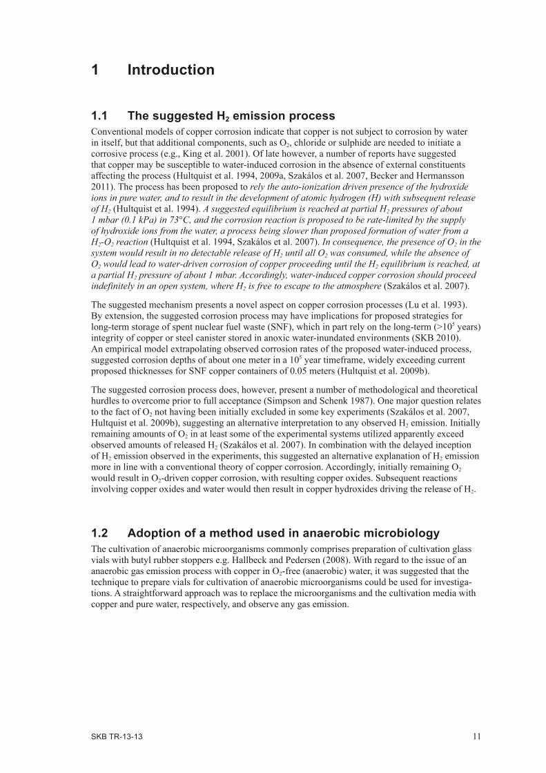
The addition of O2 at day 0 was approximately 40 nmol mL–1 which corresponded to 240 nmol per vial (Figure 2-1). The concentration of O2 was below detection (i.e. <40 nmol mL–1) after 15 days when several vials started to produce H2. After 30 days there was a significant average H2 emission in the experiment which reached an average partial pressure of 0.4 mbar after 43 days. Sampling did not cause pressure drops above what was caused by the withdrawn sample volumes which shows that the pressure problems encountered during Development Phase II (A2.3.2) could be controlled with a two-step penetration procedure. Weekly sampling occasions did reduce the vial pressure rather quickly, and it was decided to sample alternating N1 vials after 15 days to save pressure. That is the reason for why data points are missing for some vials between day 15 and 37 (Figure 2-1).

After the change of gas environment and repeated wash with the acid, H2 was produced in all vials but one after 14 days (Figure 2-2). The vial with no signs of H2 emission (N1_2:3) was O2 contami-nated due to a leak in the gas bench on the corresponding vial line. Eventually, H2 was emitted also in this vial. The average partial pressure of H2 increased linearly and was 2.2 mbar after 111 days. The two vials with fastest H2 emission in N1 was N1:4 and N1:8. These vials had the fastest H2 emission rate also in N1_2. Although this pair-wise comparison did not hold for all vials, those who did may suggest that each copper rod pairs had specific surface characters which exerted control over its H2 emission rate.

The N1 and N1_2 experiments suggested that H2 emission will not commence in the presence of O2. The experiments also showed that O2 disappeared from the gas phase which may have been due to reactions with the copper, dissolution in the water, or due to diffusion into the stopper (see A1.3.2 for details) or combinations thereof. When there was no detectable O2 in the gas phase, H2 emission started.

2.2.4 N2 – O2 treatmentThe addition of O2 at day 0 was approximately 50 nmol mL–1 which corresponded to 300 nmol per vial (Figure 2-3). The concentration of O2 was below detection (i.e. <40 nmol mL–1) after 15 days when several vials started to produce H2. Because the H2 emission was slow, and the pressure was decreasing with the number of samplings towards atmospheric pressure, analysis was halted for 40 days after day 38. At day 155 all vials had produced H2 and the average partial pressure reached 2.4 mbar. Again, sampling did not cause pressure drops above what was caused by the withdrawn sample volumes.

The N2 experiment results reproduced the N1 and N1_2 experimental results well and again showed that H2 emission will not commence in the presence of O2. This experiment, just like N1, showed that O2 disappeared from the gas phase which most likely was due to reactions with the copper. When there was no detectable O2 in the gas phase, H2 emission started.

SK

B TR

-13-13 19

0 5 10 15 20 25 30 35 40 45

Time (days)

0.0

0.2

0.4

0.6

0.8

1.0

1.2

0 5 10 15 20 25 30 35 40 45

Time (days)

0

20

40

60

80

100

N1:1 N1:2 N1:3 N1:4 N1:5 N1:6 N1:7 N1:8 N1:9 N1:10

0 5 10 15 20 25 30 35 40 45

Time (days)

100

120

140

160

180

200

N1:1 N1:2 N1:3 N1:4 N1:5 N1:6 N1:7 N1:8 N1:9 N1:10

0 5 10 15 20 25 30 35 40 45

Time (days)

0.0

0.2

0.4

0.6

0.8

1.0

1.2

N1:1 N1:2 N1:3 N1:4 N1:5 N1:6 N1:7 N1:8 N1:9 N1:10

H2 (

mba

r)

H2 (

mba

r)

O2 (

nmol

mL-1

)

P afte

r inj

. (kP

a)

Figure 2-1. Experiment N1. The partial pressure of H2 in each vial (top left); the average partial pressure of H2 in all vials, bars show standard deviation (top right); the analyzed amount of O2 per mL in each vial (bottom left), data below 40 nmol O2 mL–1 is from air contamination during injection, see 2.2.2 for details and the pressure in each vial after each sampling occasion (bottom right).

20 S

KB

TR-13-13

Figure 2-2. Experiment N1_2. The partial pressure of H2 in each vial (top left); the average partial pressure of H2 in all vials, bars show standard deviation (top right); the analyzed amount of O2 per mL in each vial (bottom left), data below 40 nmol O2 mL–1 (80 for the last sample in time) is from air contamination during injection, see 2.2.2 for details and the pressure in each vial after each sampling occasion (bottom right).

0 10 20 30 40 50 60 70 80 90 100 110

Time (days)

0.0

0.5

1.0

1.5

2.0

2.5

3.0

3.5

4.0

N1_2:1 N1_2:2 N1_2:3 N1_2:4 N1_2:5 N1_2:6 N1_2:7 N1_2:8 N1_2:9 N1_2:10

0 10 20 30 40 50 60 70 80 90 100 110

Time (days)

0.0

0.5

1.0

1.5

2.0

2.5

3.0

0 10 20 30 40 50 60 70 80 90 100 1100

20

40

60

80

100 N1_2:1 N1_2:2 N1_2:3 N1_2:4 N1_2:5 N1_2:6 N1_2:7 N1_2:8 N1_2:9 N1_2:10

0 10 20 30 40 50 60 70 80 90 100 110100

120

140

160

180

200

N1_2:1 N1_2:2 N1_2:3 N1_2:4 N1_2:5 N1_2:6 N1_2:7 N1_2:8 N1_2:9 N1_2:10

Time (days) Time (days)

H2 (

mba

r)

H2 (

mba

r)

O2 (

nmol

mL-1

)

P afte

r inj

. (kP

a)

SK

B TR

-13-13 21

Figure 2-3. Experiment N2. The partial pressure of H2 in each vial (top left); the average partial pressure of H2 in all vials, bars show standard deviation (top right); the analyzed amount of O2 per mL in each vial (bottom left), data below 40 nmol O2 mL–1 (80 for the last sample in time) is from air contamination during injection, see 2.2.2 for details and the pressure in each vial after each sampling occasion (bottom right).

0 20 40 60 80 100 120 140 1600.0

0.5

1.0

1.5

2.0

2.5

3.0

3.5

4.0

0 20 40 60 80 100 120 140 1600

20

40

60

80

100

120 N2:1 N2:2 N2:3 N2:4 N2:5 N2:6 N2:7 N2:8 N2:9 N2:10

0 20 40 60 80 100 120 140 160100

120

140

160

180

200 N2:1 N2:2 N2:3 N2:4 N2:5 N2:6 N2:7 N2:8 N2:9 N2:10

0 20 40 60 80 100 120 140 1600.0

0.5

1.0

1.5

2.0

2.5

3.0

3.5

4.0 N2:1 N2:2 N2:3 N2:4 N2:5 N2:6 N2:7 N2:8 N2:9 N2:10

Time (days)Time (days)

Time (days) Time (days)

H2 (

mba

r)

H2 (

mba

r)

O2 (

nmol

mL-1

)

P afte

r inj

. (kP

a)

22 SKB TR-13-13

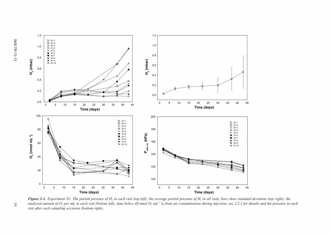
2.2.5 N3 – N2 treatment and H2 removalThere was no H2 emission in the absence of copper in vials (Figure 2-4). The O2 concentration was below the injection uncertainty limit (i.e. <40 nmol mL–1) in all sampling occasions except for day 5 when there may have been O2 present, but the data is distributed around the report limit and it is not possible to confirm absence or presence (due to air contamination from the gas bench safety valve) of O2 here. There was variability in pressure at start for unknown reasons. Occasionally, there was a problem with a safety valve in the gas bench that may have disturbed the filling of the tubes. This valve was, therefore, disconnected after experiment N4. Nevertheless, H2 emission started after day 5 and there was a linear, continuous emission of H2 in three vials for the 40 days this experiment lasted. Two vials seemed to cease to produce H2 after 34 days. Although there was a large variability in the data between vials, each vial seemed to have it own, specific H2 emission rate. When the vials were evacuated of H2 and supplied with N2 again, H2 emission continued in all five vials with copper rods (Figure 2-5).

The order of vials with respect to H2 emission rate in experiment N3_2 was withheld almost exactly as in experiment N3. Just as found in experiment N1, it appears likely that each set of two copper rods, for unknown reasons, had characters that determined how much H2 could be produced over time. Vial N3_2:3 lost pressure and appeared to be O2 contaminated. This was again due to a leak in the vial line 3 on the gas bench. The vial was later replaced. The average partial pressure of H2 was 2.0 mbar in N3 after 40 days and it became 3.1 mbar after 111 days in N3_2.

The N3 experiment showed that copper must be present in the vials to obtain H2 emission (as shown also in Development Phase I and II). It was also found that when H2 was removed from the vials, more H2 was produced. However, the experimental set-up was not exhaustive because of a rather short emission time that only allowed 2 out of 5 vials to cease the H2 emission before H2 removal.

2.2.6 N4 – O2 treatment The addition of O2 at day 0 to vials with copper rods was approximately 30 nmol mL–1 which corresponded to 180 nmol per vial (Figure 2-6). The concentration of O2 was below detection (i.e. <40 nmol mL–1) after 15 days when all five vials started to produce H2. The emission of H2 increased linearly and the standard deviation was less than 30 % of the mean value. The average partial pressure of H2 was 3.5 mbar in N4 after 86 days and it increased to 4.8 mBar after 151 days. The vials with only water had a 4 mL larger gas phase than the 6 mL gas phase above the copper rods. This difference in volume was because an equal volume of water was added – the volume of the copper was 4 mL. However, this was not optimal for interpretations and future experiments should have an equal volume of the gas phase. The total amount of gas in nmol per vial was the same for all vials, both with and without copper rods. Consequently, although it appears as if there were equal amounts of O2 mL–1 there was more O2 in the water only vials after 70 days, than in the vials with copper rods. It remains to resolve the exact fate of O2 in the vials. The N4 experiment was started relatively early in this experimental series and the technicians on the GC was still developing their injection technique and some of the decrease in O2 over time may be due to improved skills – this is valid for all experiments. However, the focus was on H2 emission and those measurements were generally flawless. The N4 experiment, like the N1 and N2 experiments, again showed H2 emission started when there was no detectable O2 in the gas phase. This experiment also showed that the variance in data can be reduced significantly compared to what was observed in Development Phase I and II. It confirmed previous results showing that the average partial pressure of H2 can approach 5 mbar in the gas phase of the vials; one vial reached more than 6 mbar.

SK

B TR

-13-13 23

Figure 2-4. Experiment N3. The partial pressure of H2 in each vial (top left); the average partial pressure of H2 in all vials, bars show standard deviation (top right); the analyzed amount of O2 per mL in each vial (bottom left), data below 40 nmol O2 mL–1 is from air contamination during injection, see 2.2.2 for details and the pressure in each vial after each sampling occasion (bottom right). Red symbols show results from vials with copper rods and water, black symbols show results from vials with water only.

0 5 10 15 20 25 30 35 40 45

0.0

0.5

1.0

1.5

2.0

2.5

3.0

3.5

4.0

4.5

0 5 10 15 20 25 30 35 40 450

20

40

60

80

100

N3:1 N3:2 N3:3 N3:4 N3:5 N3:6 N3:7 N3:8 N3:9 N3:10

0 5 10 15 20 25 30 35 40 45100

120

140

160

180

200

N3:1 N3:2 N3:3 N3:4 N3:5 N3:6 N3:7 N3:8 N3:9 N3:10

0 5 10 15 20 25 30 35 40 450.0

0.5

1.0

1.5

2.0

2.5

3.0

3.5

4.0

4.5

N3:1 N3:2 N3:3 N3:4 N3:5 N3:6 N3:7 N3:8 N3:9 N3:10

Time (days)Time (days)

Time (days) Time (days)

H2 (

mba

r)

H2 (

mba

r)

O2 (

nmol

mL-1

)

P afte

r inj

. (kP

a)

24 S

KB

TR-13-13

0 10 20 30 40 50 60 70 80 90 100 110

0

1

2

3

4

5 N3_2:1 N3_2:2 N3_2:3 N3_2:4 N3_2:5 N3_2:6 N3_2:7 N3_2:8 N3_2:9 N3_2:10

0 10 20 30 40 50 60 70 80 90 100 110

0

1

2

3

4

5

0 10 20 30 40 50 60 70 80 90 100 1100

20

40

60

80

100 N3_2:1 N3_2:2 N3_2:3 N3_2:4 N3_2:5 N3_2:6 N3_2:7 N3_2:8 N3_2:9 N3_2:10

0 10 20 30 40 50 60 70 80 90 100 11080

100

120

140

160

180

200 N3_2:1 N3_2:2 N3_2:3 N3_2:4 N3_2:5 N3_2:6 N3_2:7 N3_2:8 N3_2:9 N3_2:10

Time (days) Time (days)

Time (days) Time (days)

H2 (

mba

r)

H2 (

mba

r)

O2 (

nmol

mL-1

)

P afte

r inj

. (kP

a)

Figure 2-5. Experiment N3_2. The partial pressure of H2 in each vial (top left); the average partial pressure of H2 in all vials, bars show standard deviation (top right); the analyzed amount of O2 mL–1 in each vial (bottom left), data below 40 nmol O2 mL–1 (80 for the last sample in time) is from air contamination during injection, see 2.2.2 for details and the pressure in each vial after each sampling occasion (bottom right). Red symbols show results from vials with copper rods and water, black symbols show results from vials with water only.

SK

B TR

-13-13 25

0 20 40 60 80 100 120 140100

120

140

160

180

200 N4:1 N4:2 N4:3 N4:4 N4:5 N4:6 N4:7 N4:8 N4:9 N4:10

0 20 40 60 80 100 120 1400

20

40

60

80

100

120

140

160

180

200 N4:1 N4:2 N4:3 N4:4 N4:5 N4:6 N4:7 N4:8 N4:9 N4:10

0 20 40 60 80 100 120 140

0

1

2

3

4

5

6 N4:1 N4:2 N4:3 N4:4 N4:5 N4:6 N4:7 N4:8 N4:9 N4:10

0 20 40 60 80 100 120 140

0

1

2

3

4

5

6

7

Time (days)Time (days)

Time (days) Time (days)

H2 (

mba

r)

H2 (

mba

r)

O2 (

nmol

mL-1

)

P afte

r inj

. (kP

a)

Figure 2-6. Experiment N4. The partial pressure of H2 in each vial (top left); the average partial pressure of H2 in all vials, bars show standard deviation (top right); the analyzed amount of O2 per mL in each vial (bottom left), data below 40 nmol O2 mL–1 (80 for the last sample in time) is from air contamination during injection, see 2.2.2 for details and the pressure in each vial after each sampling occasion (bottom right). Red symbols show results from vials with copper rods and water, black symbols show results from vials with water only.

26 SKB TR-13-13

2.2.7 N5 – N2 treatment and H2 removal, stoppers in contact with waterO2 was below detection in all samples, the variability in O2 day 22 was likely caused by injection contamination (Figure 2-7). All vials emitted H2, but vials with the stoppers in contact with water produced, on average, less H2 than did vials without contact. One vial (N5:7) appeared to have a “stopper problem” that resulted in a faster pressure drop compared to all other vials and the vial was removed after day 37 due to too low pressure for analysis. Vial N5:6 was sampled repeatedly day 30 which explains the large pressure drop that day. Else, the vial pressures were well kept together over time. Again, the H2 emission rates were linear and vial specific. The vial with the fastest emission reached a hydrogen pressure of 3.6 mbar H2 after 42 days. There was on average 2.6 mbar H2 in vials with no contact between stoppers and water and 1.7 mbar H2 in vials with contact between stoppers and water. The reasons for this “stopper effect” on H2 emission were not clear. It was assumed that it could be due to traces of dish washing chemicals and, therefore, the remaining experiments were performed with new stoppers without being machine washed.

The N5_2 experiment showed that H2 emission continued with an average emission rate that was approximately similar to the average emission rate observed in N5 (Figure 2-8). Again, as observed in N3 and N3_2, the order of vials with respect to H2 emission rate in experiment N5_2 was withheld similar as in experiment N5. The average partial pressure of H2 was 2.6 mbar in N5 with new stoppers up after 40 days and it became 3.2 mbar after 99 days in N5_2.

2.2.8 N6 – N2 treatment and increased pressureThe pressure was increased and new stoppers were used, else this experiment reproduced N5. The “stopper effect” was reduced and there was no visible difference after day 50 (Figure 2-9). However, due to the pressure drops in the vials with stopper upwards, the partial pressure of H2 may be under-estimated. The reason for having stoppers downwards was to reduce problems with the pressure drops encountered in Development Phase II. This was indeed effective because in this experiment, there was pressure drops in several of the vials with stoppers up, while vials with stopper down did not have pressure drops larger than what was caused by sampling. However, it cannot be excluded that the observed pressure drops is due to leakage during stopper penetration. The reasons behind the pressure drop in N6 are not clear and it only occurred in large scale in this and the N8 experiment. It may have been caused by problems with the sampling syringes and needles. The average partial pressure of H2 was 1.9 mbar in N6 after 136 days.

2.2.9 N7 – N2 treatment, stoppers in contact with waterThis experiment reproduced the conditions in N6 and this time, there was no unexplained pressure drops (Figure 2-10). There was a small, visible effect from the stoppers on the H2 emission. The average partial pressure of H2 was 2.8 mbar in N7 after 128 days. The N7 experiment shows that it is possible to keep similar pressures in parallel vials during 8 repeated sampling occasions. Basically, exercise grows skill – this experimental set-up is very sensitive to “skills of the hand” and our technicians develop such skills experiment by experiment.

2.2.10 N8 – Acid wash effectThis experiment basically failed due to uncontrolled pressure drops (Figure 2-11). The reasons for these drops are not clear. The most likely cause for the observed pressure drops is leakage during stopper penetration. The experience from experiment N8 demonstrates that the experimental set-up and the data obtained show when an experiment fails due to O2 contamination (not a problem in N8) or uncontrolled pressure drops. Data was still collected but interpretations should be made with caution. The pressure drops were biased towards the non-acid washed copper rods. This may explain why the average partial pressure of H2 was lower compared to the vials with acid washed copper rods. The two vials with highest partial pressures of H2 had non-acid washed copper rods. This experiment, dealing with how surface treatments may influence H2 emission must be repeated flawless for proper conclusions. Because surface treatment with or without acid appeared to exert effect on H2 emission, a new experiment was started with pH adjustments.

SK

B TR

-13-13 27

Figure 2-7. Experiment N5. The partial pressure of H2 in each vial (top left); the average partial pressure of H2 in all vials, bars show standard deviation (top right); the analyzed amount of O2 per mL in each vial (bottom left), data below 40 nmol O2 mL–1 is from air contamination during injection, see 2.2.2 for details and the pressure in each vial after each sampling occasion (bottom right). Red symbols show results from vials with stoppers up and black symbols show results from vials with stoppers down in contact with the vial water.

0 5 10 15 20 25 30 35 40 45

0.0

0.5

1.0

1.5

2.0

2.5

3.0

3.5

4.0

4.5

0 5 10 15 20 25 30 35 40 450

20

40

60

80

100

N5:1 N5:2 N5:3 N5:4 N5:5 N5:6 N5:7 N5:8 N5:9 N5:10

0 5 10 15 20 25 30 35 40 45100

120

140

160

180

200

N5:1 N5:2 N5:3 N5:4 N5:5 N5:6 N5:7 N5:8 N5:9 N5:10

0 5 10 15 20 25 30 35 40 450.0

0.5

1.0

1.5

2.0

2.5

3.0

3.5

4.0

4.5

N5:1 N5:2 N5:3 N5:4 N5:5 N5:6 N5:7 N5:8 N5:9 N5:10

Time (days) Time (days)

Time (days) Time (days)

H2 (

mba

r)

H2 (

mba

r)

O2 (

nmol

mL-1

)

P afte

r inj

. (kP

a)

28 S

KB

TR-13-13

Figure 2-8. Experiment N5_2. The partial pressure of H2 in each vial (top left); the average partial pressure of H2 in all vials, bars show standard deviation (top right); the analyzed amount of O2 per mL in each vial (bottom left), data below 40 nmol O2 mL–1 (80 for the last sample in time) is from air contamination during injection, see 2.2.2 for details and the pressure in each vial after each sampling occasion (bottom right). Red symbols show results from vials with stoppers up and black symbols show results from vials with stoppers down in contact with the vial water.

0 10 20 30 40 50 60 70 80 90 1000

1

2

3

4

5 N5_2:1 N5_2:2 N5_2:3 N5_2:4 N5_2:5 N5_2:6 N5_2:7 N5_2:8 N5_2:9 N5_2:10

0 10 20 30 40 50 60 70 80 90 1000

1

2

3

4

5

6

0 10 20 30 40 50 60 70 80 90 1000

20

40

60

80

100 N5_2:1 N5_2:2 N5_2:3 N5_2:4 N5_2:5 N5_2:6 N5_2:7 N5_2:8 N5_2:9 N5_2:10

0 10 20 30 40 50 60 70 80 90 100

100

120

140

160

180

200 N5_2:1 N5_2:2 N5_2:3 N5_2:4 N5_2:5 N5_2:6 N5_2:7 N5_2:8 N5_2:9 N5_2:10

Time (days) Time (days)

Time (days) Time (days)

H2 (

mba

r)

H2 (

mba

r)

O2 (

nmol

mL-1

)

P afte

r inj

. (kP

a)

SK

B TR

-13-13 29

Figure 2-9. Experiment N6. The partial pressure of H2 in each vial (top left); the average partial pressure of H2 in all vials, bars show standard deviation (top right); the analyzed amount of O2 per mL in each vial (bottom left), data below 40 nmol O2 mL–1 (80 for the last sample in time) is from air contamination during injection, see 2.2.2 for details and the pressure in each vial after each sampling occasion (bottom right). Red symbols show results from vials with stoppers up and black symbols show results from vials with stoppers down in contact with the vial water.

0 20 40 60 80 100 120 140

0.0

1.0

2.0

3.0

4.0

0 20 40 60 80 100 120 1400

20

40

60

80

100 N6:1 N6:2 N6:3 N6:4 N6:5 N6:6 N6:7 N6:8 N6:9 N6:10

0 20 40 60 80 100 120 14080

100

120

140

160

180

200 N6:1 N6:2 N6:3 N6:4 N6:5 N6:6 N6:7 N6:8 N6:9 N6:10

0 20 40 60 80 100 120 1400.0

0.5

1.0

1.5

2.0

2.5

3.0

3.5

4.0 N6:1 N6:2 N6:3 N6:4 N6:5 N6:6 N6:7 N6:8 N6:9 N6:10

Time (days)Time (days)

Time (days) Time (days)

H2 (

mba

r)

H2 (

mba

r)

O2 (

nmol

mL-1

)

P afte

r inj

. (kP

a)

30 S

KB

TR-13-13

Figure 2-10. Experiment N7. The partial pressure of H2 in each vial (top left); the average partial pressure of H2 in all vials, bars show standard deviation (top right); the analyzed amount of O2 per mL in each vial (bottom left), data below 40 nmol O2 mL–1 (80 for the last sample in time) is from air contamination during injection, see 2.2.2 for details and the pressure in each vial after each sampling occasion (bottom right). Red symbols show results from vials with stoppers up and black symbols show results from vials with stoppers down in contact with the vial water.

0 20 40 60 80 100 120

0.0

0.5

1.0

1.5

2.0

2.5

3.0

3.5

4.0

4.5

5.0

5.5

6.0

0 20 40 60 80 100 1200

20

40

60

80

100 N7:1 N7:2 N7:3 N7:4 N7:5 N7:6 N7:7 N7:8 N7:9 N7:10

0 20 40 60 80 100 120

100

120

140

160

180

200 N7:1 N7:2 N7:3 N7:4 N7:5 N7:6 N7:7 N7:8 N7:9 N7:10

0 20 40 60 80 100 1200

1

2

3

4

5 N7:1 N7:2 N7:3 N7:4 N7:5 N7:6 N7:7 N7:8 N7:9 N7:10

Time (days) Time (days)

Time (days) Time (days)

H2 (

mba

r)

H2 (

mba

r)

O2 (

nmol

mL-1

)

P afte

r inj

. (kP

a)

SK

B TR

-13-13 31

Figure 2-11. Experiment N8. The partial pressure of H2 in each vial (top left); the average partial pressure of H2 in all vials, bars show standard deviation (top right); the analyzed amount of O2 per mL in each vial (bottom left), data below 40 nmol O2 mL–1 (80 for the last sample in time) is from air contamination during injection, see 2.2.2 for details and the pressure in each vial after each sampling occasion (bottom right). Red symbols show results from vials with acid washed copper rods, black symbols show results from vials with copper rods only washed in ethanol.

0 20 40 60 80 100 120

-1.0

0.0

1.0

2.0

3.0

4.0

5.0

6.0

0 20 40 60 80 100 1200

20

40

60

80

100 N8:1 N8:2 N8:3 N8:4 N8:5 N8:6 N8:7 N8:8 N8:9 N8:10 N8:11 N8:12 N8:13 N8:14

0 20 40 60 80 100 120

100

120

140

160

180

200 N8:1 N8:2 N8:3 N8:4 N8:5 N8:6 N8:7 N8:8 N8:9 N8:10 N8:11 N8:12 N8:13 N8:14

0 20 40 60 80 100 1200

1

2

3

4

5

6 N8:1 N8:2 N8:3 N8:4 N8:5 N8:6 N8:7 N8:8 N8:9 N8:10 N8:11 N8:12 N8:13 N8:14

Time (days) Time (days)

Time (days) Time (days)

H2 (

mba

r)

H2 (

mba

r)

O2 (

nmol

mL-1

)

P afte

r inj

. (kP

a)

32 SKB TR-13-13

2.2.11 N9 – pH adjustmentsThe vials adjusted to pH 7 with a small amount of NaOH rapidly produced H2 at the fastest rate of all experiment N1–N9 (Figure 2-12). The H2 emission in the five pH 7 vials was coherent with a stand-ard deviation of < 10% after 21 days and 20% after 32 days. The average H2 emission in the pH 9 treatment closely followed that of the pH 7 treatment but with a somewhat larger standard deviation. Lowering the pH to 2–3 resulted in a much slower average H2 emission compared to pH 7 and 9–10. The O2 content were far below the detection limit and all but five vials had excellent pressure curves day 21. The most likely cause for the observed pressure drops is leakage during stopper penetration day 21. The average partial pressures of H2 was 4.5 mbar in N9 pH 7, 2.7 mbar in pH 9–10 and 3.1 mbar in pH 2–3 after 101 days.

2.3 DiscussionDevelopment Phase II confirmed that the method could be used to follow H2 emission from copper in pure anoxic water. However, there were technical shortcomings that had to be dealt with before the method could be regarded as developed to a state that allow further investigations of the mecha-nisms behind the H2 emissions. The most important issues were to eliminate uncontrolled pressure drops in the vials and to understand how the variance of vials with seemingly identical set-ups can be reduced. The variables O2 and pH was assumed to be the most important factors.

2.3.1 Understanding the influence of O2

Development Phase I and II results (Appendix 1 and 2) suggested that O2 reduced, inhibited or delayed the H2 emission from copper. In the method validation phase, we further developed our analysis of O2 and managed to make controlled additions of O2 better than in Development Phase I and II. In Development Phase I, there was a contamination with O2 from the stopper and this problem was solved during Development Phase II. Method validation results showed that H2 emission was inhibited when there were detectable amounts of O2 in the gas phase of the vials (Experiments N1, N3 and N4). The effect was reversible because H2 emission started when O2 became below the detec-tion limit. Most likely, the disappearance of O2 was due to reactions with the copper rod surfaces.

2.3.2 Reducing uncontrolled pressure dropsUncontrolled pressure drops occurred in Development Phase II and they were deduced to the penetrations of the rubber stoppers. This problem was mitigated during the method validation phase, but occasionally, such pressure drops did occur. The way around is to continue to develop a gentle sampling method and to produce enough vials to allow for deletion of data from vials that fail a controlled pressure decrease.

2.3.3 Reducing variance of identical vialsContinuous improvement of the preparation and analysis procedures eventually reduced the variance between vials. The data variance from parallel vials was smaller in the Method validation phase than in Development phase II. It appeared likely that the variance was due to surface specific characters of the copper rods. This was assumed because sets of vials from which H2 were removed continued to emit H2 in the same rate order as was observed before H2 removal. The only possible variance factor for the copper rods could be the cleaning procedure that may have carried over trace amounts of ethanol and acid – i.e. such cleaning chemicals that was not washed off in the 4 washing steps. The volume of wash water was, therefore, increased 4 times after the N8 experiment (Table 2-1) but there was no obvious effect noted. Although we use clean water, CO2 from the atmosphere and the box environment tends to lower pH of pure water and this effect must, therefore be mitigated. Therefore, when pH was set to 7 with a small amount of NaOH, data from five parallel vials became very coherent with a standard deviation of less than 10 %. This observation may indicate that the pH of the water and the copper rods influences the H2 emission rate. When pH was lowered to 2–3 with HCl, the emission rate decreased; that decrease could be caused by pH or chloride ions or both. The investigation of the influence of a low pH will require a buffer or an acid that cannot react with the copper rod, or complex with copper ions.

SK

B TR

-13-13 33

Figure 2-12. Experiment N9. The partial pressure of H2 in each vial (top left); the average partial pressure of H2 in all vials, bars show standard deviation (top right); the analyzed amount of O2 per mL in each vial (bottom left), data below 40 nmol O2 mL–1 (80 for the last sample in time) is from air contamination during injection, see 2.2.2 for details and the pressure in each vial after each sampling occasion (bottom right). Black symbols show pH 7, red symbols show pH 9–10 and blue symbols show pH 2–3.

0 10 20 30 40 50 60 70 80 90 1000

1

2

3

4

5

6 N9:1 N9:2 N9:3 N9:4 N9:5 N9:6 N9:7 N9:8 N9:9 N9:10 N9:11 N9:12 N9:13 N9:14 N9:15

0 10 20 30 40 50 60 70 80 90 100

0

1

2

3

4

5 H2 mbar pH 7 H2 mbar pH 9-10 H2 mbar pH 2-3

0 10 20 30 40 50 60 70 80 90 1000

20

40

60

80

100

120 N9:1 N9:2 N9:3 N9:4 N9:5 N9:6 N9:7 N9:8 N9:9 N9:10 N9:11 N9:12 N9:13 N9:14 N9:15

0 10 20 30 40 50 60 70 80 90 100

100

120

140

160

180

200 N9:1 N9:2 N9:3 N9:4 N9:5 N9:6 N9:7 N9:8 N9:9 N9:10 N9:11 N9:12 N9:13 N9:14 N9:15

Time (days) Time (days)

Time (days) Time (days)

H2 (

mba

r)

H2 (

mba

r)

O2 (

nmol

mL-1

)

P afte

r inj

. (kP

a)

34 SKB TR-13-13

2.3.4 A method to investigate mechanisms behind H2 emission from copper in anoxic water

At the end of the method validation phase, we are confident that we have an alternative method without palladium that can be used to investigate the mechanisms behind H2 emission in O2-free pure water see chapter (3).

SKB TR-13-13 35

3 A method for the investigation of H2 emission from copper in O2-free water

3.1 Method protocolThe following methodological protocol was developed in a stepwise procedure as described in chapter 2 and Appendices 1 and 2. It can now be used for investigations of the influence of many different variables on the H2 emission process such as the effect from dissolved ions, pH and microorganisms.

3.2 Preparation of copper rods1. Copper rods measuring 100×10×2 mm, exhibiting a 15 degree angle at one end are machine cut

from O2-free, phosphorus doped copper (Cu-OFP) and engraved with running numbers.

2. Polish the copper rods using an electric grinder (Bosch PBS 7 AE; Hornbach Gothenburg, Sweden) with sanding belt of grain size 150, (kwb tools, art.nr 9119-10 Hornbach, Gothenburg Sweden). Finish by hand with fine sanding paper of grain size P600 (Hornbach Gothenburg, Sweden), see Figure 3-1 and Figure 3-2. Make sure all signs of oxidation spots are removed and all surfaces are shiny of clean and pure copper.

3. Immediately place the polished copper rods in a plastic container filled with O2-free >70 % ethanol (Scharlau) to cover all rods, and close the lid. Immediately place the container with the copper rods in an anaerobic environment.

4. To prevent oxidation of copper rods in contact with oxygen after the grinding step the following preparation of copper rods is performed in an anaerobic glove box environment (COY Laboratory Products, MI, USA). All equipment and tools should be placed in the anaerobic environment before the preparation starts.

5. To remove grease and impurities, place the copper rods in an Ultrasonic cleaner (Branson B200) containing 300 mL >70 % ethanol (Scharlau) to cover all rods. Run the cleaning program during 5 minutes, see Figure 3-3.

6. Use a clean tweezers to transfer the copper rods and sequentially wash each rod twice in a glass beaker containing 400 mL autoclave sterilized, anoxic Millipore analytical grade water.

7. Acid leach and remove possibly remaining oxidation products from the copper rods, by placing the copper rods in a beaker containing gently stirred 250 mL 50 g L–1 sulfamic acid (Aminosulfonic acid, H2NSO3H) (cat.nr. 24,277-2 Sigma-Aldrich) for 10 minutes, according to procedures for chemical cleaning of copper in ISO 8407:2010 – Corrosion of metals and alloys – Removal of corrosion products from corrosion test specimens (ISO 847:2009, IDT), see Figure 3-4.

8. Finish the procedure by using a clean tweezers and wash four times sequentially by washing each rod in glass beakers containing 400 mL autoclave sterilized, anoxic analytical grade water at pH 7. Sulfamic acid should be completely washed away from the copper rods.

9. Let the copper rods dry on a lint-free Kleenex.

10. Place one copper rod in a 26 mL gas tight, anaerobic borosilicate experimental vial, (Product #2048-18150, Bellco Glass Inc., NJ, USA) with the angled end pointing downwards. Place one more copper rod in the same vial, with the angled end pointing upwards. Make sure that the two rods are placed anti-parallel, and there is a gap between the copper rods. Place all copper rods similarly in pairs in each vial.

11. Seal the vials with matching impermeable butyl rubber stoppers (Bellco, Product #2048-117800).

36 SKB TR-13-13

12. Remove sealed vials from the anaerobic glove box. Cap the sealed vials with an aluminium ring (Chromacol cat.nr 9112010746) by clamping with pliers. Make sure the aluminum ring is completely tightened by marks from the clamping visible around the ring, see Figure 3-5.

13. Weigh and name each vial, link the identity with numbers on the copper rods.

14. Evacuate the vials using a Gas bench, see Figure 3-6. Evacuate down to <0.9 kPa and fill up with Instrumental N2 to 200 kPa. Repeat the evacuation and filling procedure five more times, to make sure the vials are completely anaerobic, and leave by filling with Instrumental N2 to 200 kPa.

3.3 Preparation of water for filling the vials with copper rods15. Purge 2 litres of AGW-water of O2 by bubbling with instrumental N2 for an hour in a gas tight

glass flask with a gas-inlet. Keep the lid slightly open to let gas escape. (Butler et al. 1994), see Figure 3-7.

16. Sterilize the flask with water, all equipment and gas lines, by autoclaving at 121°C and 220 kPa for 15 minutes.

17. Place the sterilized flask with water on ice and reattach the flask equipment to gas lines with Instrumental N2.

18. Purge water with Instrumental N2 for another hour, to remove any remaining O2 through the slightly open lid.

19. Close the lid on the flask and increase the inlet pressure of Instrumental N2 to the flask, to 200 kPa. By the increased pressure, water is forced through the filling line of the flask. Take out some water from the filling line and measure pH. Adjust to 7 by adding 1 M NaOH if pH is lower than approximately 7.

20. Use sterile N2-rinsed needle attached to the filling vial. Penetrate each rubber stopper with a two-step technique, by pausing for a few seconds with the needle halfway through the rubber stopper, both on the way into and out of the vial. This to prevent air from leaking into the vial.

21. Fill each vial with 16 mL of the sterilized anoxic water. The copper rods in each vial should be completely covered by water. Leave a gas volume of about 6 mL in each vial, see Figure 3-8.

22. To compute the exact amount of water added, (and thus the exact remaining gas volume) the filled vials should be weighed one more time.

23. Immediately after water addition, the gas phase in the vials should be evacuated and filled with Instrumental N2, using a Gas bench. Evacuate down to <0.9 kPa and finish for 90 seconds after that gas bubbles appears in the water. Gas bubbles are due to water starting to boil when vacuum lowers its boiling point. Fill up with Instrumental N2 to 120 kPa. Repeat the evacuation and filling procedure five more times, and finish by filling with about 200 kPa Instrumental N2.

24. Place the vials in an anaerobic jar and close the lid. Connect the anaerobic jar with gas lines to the Gas bench and evacuate down to <0.9 kPa followed by filling with Instrumental N2 up to 120 kPa. Repeat the evacuation and filling procedure two more times and leave by filling with Instrumental N2 to 120 kPa, to make sure the atmosphere surrounding the vials in anaerobic jar is O2-free, see Figure 3-9. Place at 70°C in a heating furnace (Binder, USA) and incubate until time for analysis.

SKB TR-13-13 37

3.4 Analysis25. At defined time intervals, the amounts of O2 and H2 in the vials are analyzed using a Bruker

450 gas chromatograph (GC) equipped with a CP7355 PoraBOND Q 50m x 0.53mm ID and a CP7536 MOLSIEVE 5A PLOT 25m x 0.32mm ID and a Pulsed Discharge Helium Ionization Detector (PDHID) (Bruker Daltonics Scandinavia AB, Vallgatan 5, SE-17067 Solna, Sweden). Bruker GC 450 (Bruker, Lund Sweden).

26. Sampling is made using a 250 µL Hamilton syringe (Scantec, Sweden) with a 55 mm needle (Genetec, Sweden).

27. Remove the anaerobic jar from the 70°C heating furnace and cool to room temperature a few hours before analysis.

28. Before analyzing samples, routine is always to control the quality and reliability of the analytical method. Test the performance of sampling and condition of the instrument by injecting the sample carrier gas, as for this method is helium (AGA, Sweden). Rinse the Hamilton syringe three times with helium, and inject 100 µL of helium and analyze. When the results are approved, perform another test of the instrument.

29. Again rinse syringe three times with helium, and inject 100 µL of the specific calibration gas with known amounts of O2 and H2 (Air Liquide, Malmö Sweden). Check that the analysis parameters for the calibration gas are approved before starting to analyze the samples.

30. Always rinse the Hamilton syringe with helium before sampling, to remove any remaining gas from air and the previous sample. At sampling, use the two-step technique when the needle penetrates through the stopper, both into and out of the vial.

31. Sample approximately 120 µL of the gas phase in each vial and press out until 100 µL of gas sample is left in the syringe. Immediately inject the sample to the gas chromatograph and start analyzing, see Figure 3-10 and Figure 3-11. Injection volume is shifted from 100 to 50 µL when the H2 partial pressure approaches 3 mBar.

32. Check the results of the run and that all parameters are approved. If not, rerun sample.

33. After the analysis, use the pressure gauge to monitor the pressure in the vials, see Figure 3-12.

34. Place the analyzed vials back into the anaerobic jar, evacuate and fill 3 times with 120 kPa N2 and leave them in the 70°C heating furnace until it is time for next analysis.

3.5 Photographic documentationPhoto documentation of the method described above.

38 SKB TR-13-13

Figure 3-1. Grinding surfaces of copper rod, starting with the grinder and then by hand.

Figure 3-2. The upper part of the copper rod has shiny metallic surface of pure copper.

SKB TR-13-13 39

Figure 3-3. Ultrasonic cleaning of copper rods in the anaerobic box.

Figure 3-4. Acid leaching of copper rods in the anaerobic box.

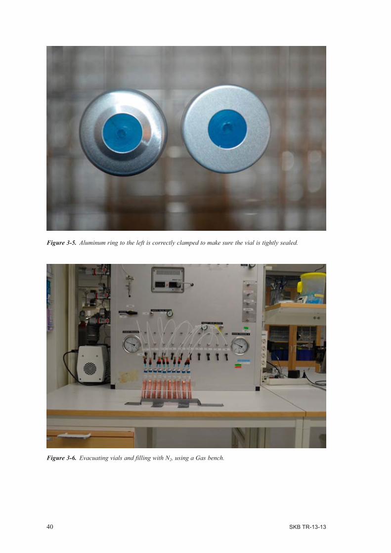
40 SKB TR-13-13

Figure 3-5. Aluminum ring to the left is correctly clamped to make sure the vial is tightly sealed.

Figure 3-6. Evacuating vials and filling with N2, using a Gas bench.

SKB TR-13-13 41

Figure 3-7. Preparing anoxic water, purge with N2.

Figure 3-8. Vials containing copper rods, filled with 16 mL water.

42 SKB TR-13-13

Figure 3-9. The anaerobic jars are evacuated and filled with N2 at the Gas bench.

Figure 3-10. Sampling from a vial with copper rods and water.

SKB TR-13-13 43

Figure 3-11. Injecting the gas sample for analysis with the GC450.

Figure 3-12. Measurement of pressure in vial after analysis.

SKB TR-13-13 45

References

SKB’s (Svensk Kärnbränslehantering AB) publications can be found at www.skb.se/publications.

Becker R, Hermansson H-P, 2011. Evolution of hydrogen by copper in ultrapure water without dissolved oxygen. Report 2011:34, Strålsäkerhetsmyndigheten (Swedish Radiation Safety Authority).

Brandrup J, Immergut E H, Grulke E A (eds), 1999. Polymer handbook. 4th ed. New York: Wiley.

Butler I B, Schoonen M A A, Rickard D T, 1994. Removal of dissolved oxygen from water: a comparison of four common techniques. Talanta 41, 211–215.

De Brabandere L, Thamdrup B, Revsbech N P, Foadi R, 2012. A critical assessment of the ocurrence and extend of oxygen contamination during anaerobic incubation utilizing commercially available vials. Journal of Microbiologica Methods 88, 147–154.

Hallbeck L, Pedersen K, 2008. Characterization of microbial processes in deep aquifers of the Fennoscandian Shield. Applied Geochemistry 23, 1796–1819.

Hultquist G, Gråsjö L, Lu Q, Åkermark T, 1994. The analysis of gas consumption in the reaction of Fe and Cu in H2

16O/H218O/O2 gas mixtures. Corrosion Science 36, 1459–1471.

Hultquist G, Szakálos P, Graham M J, Belonoshko A B, Sproule G I, Gråsjö L, Dorogokupets P, Danilov B, Aastrup T, Wikmark G, Chuah G-K, Eriksson J-C, Rosengren A, 2009a. Water corrodes copper. Catalysis Letters 132, 311–316.

Hultquist G, Szakálos P, Graham M J, Sproule G I, Wikmark G, 2009b. Detection of hydrogen in corrosion of copper in pure water. In Proceedings of the 17th International Corrosion Congress, Las Vegas, NV, 6–10 October 2008. Paper No 3884. Houston, TX: NACE International.

Hultquist G, Graham M J, Szakálos P, Sproule G I, Rosengren A, Gråsjö L, 2011. Hydrogen gas production during corrosion of copper by water. Corrosion Science 53, 310–319.

Hungate R E, Smith W, Clarke R T J, 1966. Suitability of butyl rubber stoppers for closing anaerobic roll culture tubes. Journal of Bacteriology 91, 908–909.

King F, Ahonen L, Taxén C, Vuorinen U, Werme L, 2001. Copper corrosion under expected conditions in a deep geologic repository. SKB TR-01-23, Svensk Kärnbränslehantering AB.

Ladebeck J R, Wagner J P, 2003. Catalyst development for water-gas shift. In Vielstich W, Lamm A, Gastiger H A (eds). Handbook of fuel cells: fundamentals, technology and applications. Vol 3, Part 2. Chichester: Wiley, 190–201.

Lu Q, Hultquist G, Tan K L, Åkermark T, 1993. A calculation method for analysis of SIMS spectra from oxidation of metals in H2

16O/H218O/16O2 gas mixtures. Surface and Interface Analysis

20, 645–650.

Massey L K, 2003. Bytyl rubber. In Permeability properties of plastics and elastomers: a guide to packaging and barrier materials. 2nd ed. New York: William Andrew Publishing, 459–463.

Pedersen K, Arlinger J, Eriksson S, Hallbeck A, Hallbeck L, Johansson J, 2008. Numbers, biomass and cultivable diversity of microbial populations relate to depth and borehole-specific con-ditions in groundwater from depths of 4–450 m in Olkiluoto, Finland. The ISME Journal 2, 760–775.

Simpson J P, Schenk R, 1987. Hydrogen evolution from corrosion of pure copper. Corrosion Science 27, 1365–1370.

SKB, 2010. Design and production of the KBS-3 repository. SKB TR-10-12, Svensk Kärnbränslehantering AB.

Szakálos P, Hultquist G, Wikmark G, 2007. Corrosion of copper by water. Electrochemical and Solid-State Letters 10, C63–C67.

Van Amerongen G J, 1946. The permeability of different rubbers to gases and its relation to diffusivity and solubility. Journal of Applied Physics 17, 972–985.

SKB TR-13-13 47

Appendix 1

Development Phase IA1.1 Materials and MethodsA1.1.1 Pilot experiments 1 and 2Two pilot experiments were performed to design an experimental configuration that addressed the hypotheses of this work (1.1). In the first test, the effect from two different O2 amounts was analyzed. O2 amounts of 420 nmol and 4,600 nmol were tested on copper rods for 24 days. It was found that 420 nmol per vial produced visible dark-black copper oxides that became densely black at 4,600 nmol per vial (Figure A1-1). The gas (42 µmol L–1 O2) resulting in 420 nmol O2 per vial with a 5 mL gas phase was selected for the experiments. In a second pilot test, details in the procedures were tested with a total of 27 vials in all types of configurations to be used to confirm that all protocols and analytical procedures worked as planned (data not shown).

Figure A1-1. Copper rods from pilot test one exposed to varying amount of O2. From left to right, 0 nmol O2 (vials 1–3). 420 nmol O2 (vials 4–6) and 4,600 nmol O2 (vials 7–9).

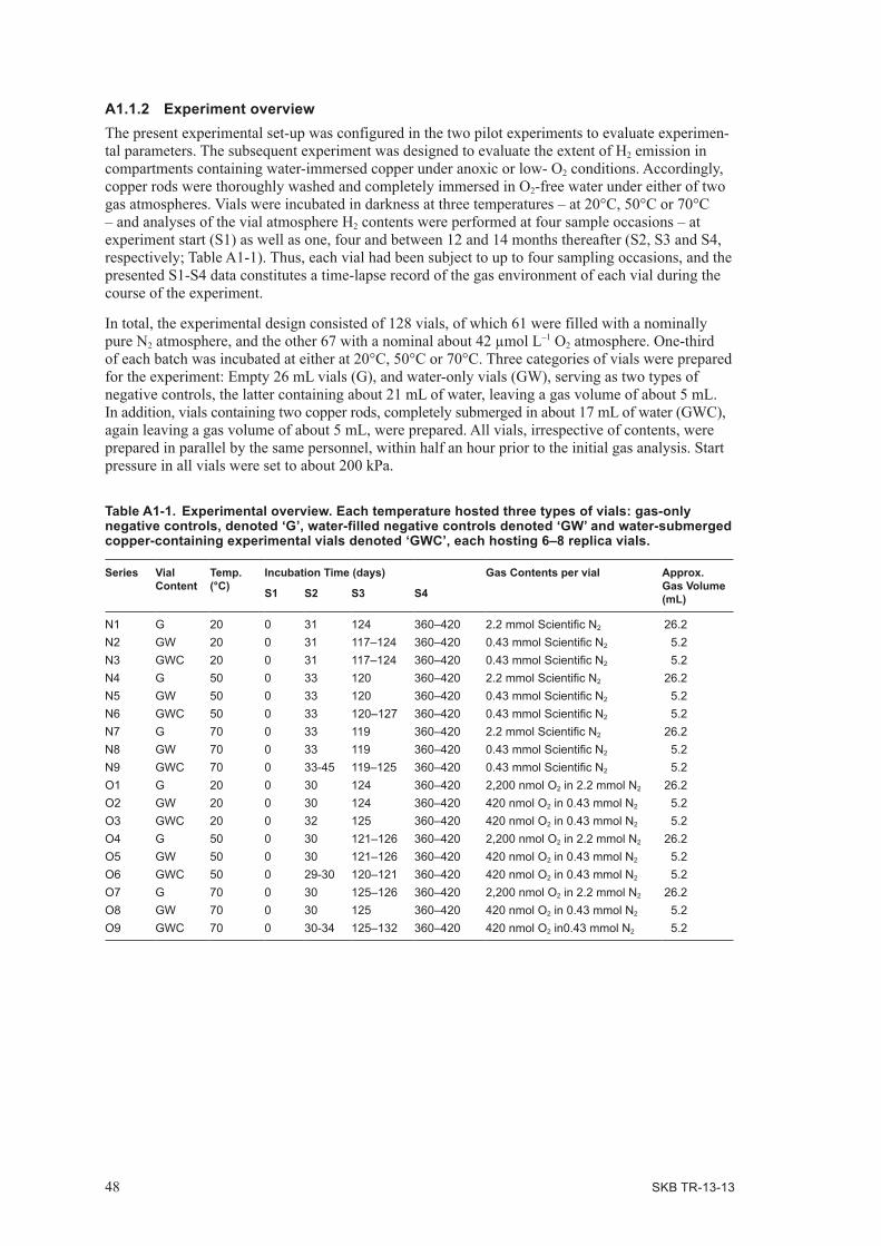
48 SKB TR-13-13

A1.1.2 Experiment overviewThe present experimental set-up was configured in the two pilot experiments to evaluate experimen-tal parameters. The subsequent experiment was designed to evaluate the extent of H2 emission in compartments containing water-immersed copper under anoxic or low- O2 conditions. Accordingly, copper rods were thoroughly washed and completely immersed in O2-free water under either of two gas atmospheres. Vials were incubated in darkness at three temperatures – at 20°C, 50°C or 70°C – and analyses of the vial atmosphere H2 contents were performed at four sample occasions – at experiment start (S1) as well as one, four and between 12 and 14 months thereafter (S2, S3 and S4, respectively; Table A1-1). Thus, each vial had been subject to up to four sampling occasions, and the presented S1-S4 data constitutes a time-lapse record of the gas environment of each vial during the course of the experiment.

In total, the experimental design consisted of 128 vials, of which 61 were filled with a nominally pure N2 atmosphere, and the other 67 with a nominal about 42 µmol L–1 O2 atmosphere. One-third of each batch was incubated at either at 20°C, 50°C or 70°C. Three categories of vials were prepared for the experiment: Empty 26 mL vials (G), and water-only vials (GW), serving as two types of negative controls, the latter containing about 21 mL of water, leaving a gas volume of about 5 mL. In addition, vials containing two copper rods, completely submerged in about 17 mL of water (GWC), again leaving a gas volume of about 5 mL, were prepared. All vials, irrespective of contents, were prepared in parallel by the same personnel, within half an hour prior to the initial gas analysis. Start pressure in all vials were set to about 200 kPa.

Table A1-1. Experimental overview. Each temperature hosted three types of vials: gas-only negative controls, denoted ‘G’, water-filled negative controls denoted ‘GW’ and water-submerged copper-containing experimental vials denoted ‘GWC’, each hosting 6–8 replica vials.

Series Vial Content

Temp. (°C)

Incubation Time (days) Gas Contents per vial Approx. Gas Volume (mL)S1 S2 S3 S4

N1 G 20 0 31 124 360–420 2.2 mmol Scientific N2 26.2N2 GW 20 0 31 117–124 360–420 0.43 mmol Scientific N2 5.2N3 GWC 20 0 31 117–124 360–420 0.43 mmol Scientific N2 5.2N4 G 50 0 33 120 360–420 2.2 mmol Scientific N2 26.2N5 GW 50 0 33 120 360–420 0.43 mmol Scientific N2 5.2N6 GWC 50 0 33 120–127 360–420 0.43 mmol Scientific N2 5.2N7 G 70 0 33 119 360–420 2.2 mmol Scientific N2 26.2N8 GW 70 0 33 119 360–420 0.43 mmol Scientific N2 5.2N9 GWC 70 0 33-45 119–125 360–420 0.43 mmol Scientific N2 5.2O1 G 20 0 30 124 360–420 2,200 nmol O2 in 2.2 mmol N2 26.2O2 GW 20 0 30 124 360–420 420 nmol O2 in 0.43 mmol N2 5.2O3 GWC 20 0 32 125 360–420 420 nmol O2 in 0.43 mmol N2 5.2O4 G 50 0 30 121–126 360–420 2,200 nmol O2 in 2.2 mmol N2 26.2O5 GW 50 0 30 121–126 360–420 420 nmol O2 in 0.43 mmol N2 5.2O6 GWC 50 0 29-30 120–121 360–420 420 nmol O2 in 0.43 mmol N2 5.2O7 G 70 0 30 125–126 360–420 2,200 nmol O2 in 2.2 mmol N2 26.2O8 GW 70 0 30 125 360–420 420 nmol O2 in 0.43 mmol N2 5.2O9 GWC 70 0 30-34 125–132 360–420 420 nmol O2 in0.43 mmol N2 5.2

SKB TR-13-13 49

A1.1.3 Experimental preparationsCopper rodsCopper rods measuring 100×10×2 mm, exhibiting a 15 degree angle at one end (Figure A1-2) were machine cut from O2-free, phosphorus doped copper (Cu-OFP) and engraved with running numbers. Copper rods were subsequently stored until experiment start, immersed in 99% ethanol in a closed vessel, placed in an anaerobic glove box environment (COY Laboratory Products, MI, USA).

All solutions used during preparations were sterilized in autoclave at 121°C for 15 minutes and, where applicable, prepared using Millipore Direct-Q purified water. In addition, all solutions used were gassed prior to use by thorough bubbling with N2 directly after sterilization. All handling was performed using clean, sterilized gloves and tweezers.

26 mL gas tight, anaerobic borosilicate experimental vials (Product #2048-18150, Bellco Glass Inc., NJ, USA) and matching impermeable butyl rubber stoppers (Product #2048-117800) were immersed in water, autoclaved at 121°C for 20 minutes and placed under sterile conditions over at least 7 days in an anaerobic glove box utilizing an O2-free N2 atmosphere containing <5% CO2 and <3.5% H2. In the anaerobic box, copper rods were withdrawn from storage, placed in 70% ethanol in sonicator bath and incubated for 5 minutes to remove surface contaminants. Rods were extracted from the sonicator bath and washed twice sequentially in 250 mL water and placed in a 50 g L–1 sulfamic acid bath during 10 minutes to remove any corrosion products present on copper rod surfaces according to ISO 8407:2009 – Corrosion of metals and alloys – Removal of corrosion products from corrosion test specimens. Remaining acid from the acid bath was allowed to drain from the copper rods during a one-minute incubation on lint-free paper. Subsequently, copper rods were washed four times sequentially in 550 mL Millipore Direct-Q water, allowed to dry on lint-free paper and then placed pair wise in antiparallel orientation in the experimental vials.

Figure A1-2. Copper rod design with 15 degree angle at one side to avoid contact between the rod surfaces.

50 SKB TR-13-13

Following positioning of copper rods, experimental vials were sealed using butyl rubber stoppers coated on the upper lateral edges with a thin layer Molycote 44 medium high temperature grease (Dow Corning GmbH, Wiesbaden, Germany). Sealed vials were capped with an aluminium ring and stored in the anaerobic box until evacuation and water application. Exact inner volume of capped, sealed experimental vials was 26.23 mL.

Sealed vials were removed from the anaerobic glove box and immediately evacuated three times down to <2.0 kPa. Vials were filled with about 120 kPa Scientific N2 between evacuations. Following the third evacuation, vials were left at <2.0 kPa. Theoretical H2 content of the vials would at this point be <40 pmol. Vials targeted for gas-only filling were then immediately filled with either Scientific N2 or 42 µmol L–1 O2 in Scientific N2 to a total pressure of about 200 kPa. Vials targeted for water negative controls and copper containing experimental vials were weighed, filled with about 21 or 17 mL autoclave sterilized, anoxic Millipore Direct-Q water that had been purged with N2 for 1 hour (Butler et al. 1994) and then weighed again, in order to procure the exact amount of water added (and thus the exact remaining gas volume). All fillings were made using thoroughly sterilized and N2-rinsed equipment and gas lines.

Immediately following water additions, vials were filled with either Scientific N2 or 42 µmol L–1 O2, to a total pressure of about 200 kPa. Following gas filling, vials were immediately taken to analysis S1, where gas pressure, H2 content and O2 content was determined. Subsequent to analyses, vials were incubated in darkness at their respective temperature. In order to facilitate gas diffusion and ensure an even mixing of gas throughout the liquid volume, vial contents in water-containing vials were lightly mixed twice a week by gently turning vials upside down five times.

Due to an overproduction of vials during sample preparations, some series contained up to eight replicates, rather than the six planned for in the experimental set-up. Similarly, due to preparation and sampling errors, some series exhibited less than six replicate samples.

pHpH of water added to negative controls and copper-containing experimental vials was determined using a Checker pH-meter (Hanna Instruments Inc., RI, USA), calibrated at pH 4.0 and pH 7.0 using standard pH calibration solutions. pH was determined by adding 100 µL, 3 M KCl to 10 mL of the sterile, N2-bubbled Millipore Direct-Q water used for vial fillings. pH-measurements were performed in six replicates, in immediate connection to filling of vials, on subsamples of water used for vial filling. Thus, pH was only measured during vial preparation (in immediate connection to S1), not during subsequent samplings (S2–S4).

pH ranged from 5.86 up to 6.16 in the analyzed vials.

Gas analysesGas sampling and analyses were initiated by allowing all vials to cool to room temperature. All vials, needles and equipment used were thoroughly flushed with Scientific N2 prior to attachment or inser-tion into experimental or control vials. All sampling was performed using an identical method. First, a pressure gauge-attached needle was inserted into the gas volume and initial pressure was noted. The pressure gauge remained attached throughout sampling to allow for continuous monitoring of pressure. Second, a 50–250 µL sample was extracted and immediately injected into the GC-injector for O2 analysis. Third, a 200 µL sample was extracted, diluted to 10 mL using Scientific N2 and injected for H2 and CO analysis. Finally, the pressure gauge needle was detached. Post-sampling pressure was noted following each gas extraction. The analyses were time consuming which resulted in up to 10 days sampling and analysis intervals for each sample occasion. From each series (N1, N2…, O1, O2…), one replicate sample was excluded from sampling at S1 and S2, being sampled only at S3 and S4, to control for putative sampling related artefacts. The sample occasion S4 was initiated by cooling the vials to room temperature after 360 days, but the analyses did not commence until after about 420 days.

SKB TR-13-13 51

H2 concentrations below 8.3 µmol L–1 and all CO analyses were performed on a Kappa-5/E-002 analyzer gas chromatograph (AMTEK, USA), equipped with a 31×0.1 inch stainless steel Molesieve 5A column attached to a reductive gas detector (RGD), using Scientific N2 as carrier gas. H2 and CO quantifications were calibrated using a one-point calibration at 100 nmol L–1 using diluted 1 µmol L–1 H2 + 1 µmol L–1 CO (in N2) calibration gas (Special Gas 4, Linde AG, Germany). At regular intervals during analyses, quantification control samples were run in order to monitor instrument quantification consistency. The detection limit for H2 and CO was 1 pmol, corresponding to 20 pL per 200 µL sample = 4 nmol L–1.

H2 concentrations above 8.3 µmol L–1 in S2 and S3 as well as all O2 analyses in S1–S3 were performed on a Varian 3400CX gas chromatograph (Agilent Technologies Inc., CA, USA). H2 and O2 were separated using a Porapak Q column (2 m×1/8 inch) serially connected to a Molesieve 5A column (6 m×1/8 inch) using either Ar or He as carrier gas for H2 and O2, respectively. The Molesieve 5A column did not separate O2 from Ar which means that this analysis showed the sum of O2 and Ar. Gases were detected using a thermal conductivity detector (TCD) at detector temperature 120°C with a filament temperature of 250°C. H2 quantification was calibrated between 1.3–6.1 µmol using 10 µmol L–1 H2 (in N2). O2 quantification was calibrated in the interval 10–600 nmol using 455 µmol L–1 Ar free O2 (in N2) calibration gas (Special Gas 1, Linde AG, Germany). At regular intervals during analyses, control samples were run in order to monitor instrument consistency. The detection limit for O2 was 1 nmol corresponding to 20 nL per 250 µL sample or 3.3 µmol L–1.

Analyses at the fourth sampling occasion, S4 (420 days), were performed on a Varian CP-3800 gas chromatograph (Agilent Technologies Inc., CA, USA). On this instrument, O2 and Ar were separated with a 30 m high resolution capillary column (Bruker, SELECT PERMANENT GASES/CO2 HR, CP7430) using He as carrier gas. The gases were detected using a thermal conductivity detector (TCD) at detector temperature 120°C with a filament temperature of 220°C and a column temperature of 45°C. O2 and Ar quantification was calibrated in the interval 10–600 nmol using 42, 420, 840 µmol L–1 O2 (in N2) calibration gas (Special Gas 1, Linde AG, Germany). At regular intervals during analyses, control samples were run in order to monitor instrument consistency. The detection limits for O2 and Ar were 1 nmol corresponding to 20 nL per 250 µL sample or 3.3 µmol L–1. At regular intervals, carrier gas (He) was injected to determine the injection error due to air captured in the syringe needle during transfer of the sample to the injector. It was found that about 0.5 mL air i.e. 0.l mL O2 were captured. This amount was subtracted from the output from the chromatograph before further data treatment was performed. A similar error was found for the 3400CX chromatograph and it was subtracted as well.

Finally, CO2 was analyzed after about 480 days using the flame ionisation detector on the Varian CX3400 chromatograph using a Porapak Q column (2 m×1/8 inch) serially connected to a nickel methanizer. At the same time carbon monoxide was analyzed in some of the GWC vials that had concentrations above the detection limit for the KAPPA-5 analyser at day 420.

Gas sampling and analyses were initiated by allowing all vials to cool to room temperature. All vials, needles and equipment used were thoroughly flushed with Scientific N2 prior to attachment or inser-tion into experimental or control vials. All sampling was performed using an identical method. First, a pressure gauge-attached needle was inserted into the gas volume and initial pressure was noted. The pressure gauge remained attached throughout sampling to allow for continuous monitoring of pressure. Second, a 50–250 µL sample was extracted and immediately injected into the GC-injector for O2 analysis. Third, a 200 µL sample was extracted, diluted to 10 mL using Scientific N2 and injected for H2 (and CO) analysis. Finally, the pressure gauge needle was detached. Post-sampling pressure was noted following each gas extraction.

A1.1.4 Copper analysis24 GWC vials and 12 GW vials were selected for analysis of dissolved copper. The vials were sent to ALS Scandinavica AB, Luleå for analysis. The method is accredited for drinking water and the analysis protocol denoted V-2, elements in water, was applied. This method had a detection limit of 10 mg Cu L–1. Briefly, the vials were opened and the copper rods were removed and the water was acidified and analyzed.

52 SKB TR-13-13

A1.1.5 H2 diffusion testA total of 10 vials were prepared as described above and filled with a gas mix containing 1 µmol L–1 H2 and 1 µmol L–1 CO in N2 (Special Gas 4, Linde AG, Germany). They were incubated at 70°C and analyzed for H2 after 1 month. The average H2 concentration decrease was 2.8 % of the start concentration. In other words, H2 did slowly diffuse out of the vials.

A1.2 ResultsA1.2.1 O2 in vialsAn unexpected technical problem was encountered in that the laboratory received a batch of Hamilton syringe needles that repeatedly broke when samples were withdrawn from the vials through the butyl rubber stopper. This problem caused large variability for O2 in some vial series from sample occasions S1 to S3. Part of the error was due to uncertainties of injections on the chro-matograph; atmospheric O2 contamination may have occurred in some cases. Additionally, there was an increased risk that some atmospheric O2 contamination reached the vials when the needles broke. This problem did not influence the H2 analyses and new and good needles were obtained before the S4 sampling occasion.

General observations for all treatmentsThere was a decreasing trend of O2 in all vials between days 0 and 30. Thereafter, the amount of O2 started to increase in most of the G and GW vials, but not in the GWC vials.

Observations specific for each treatmentThe G vials had more O2 in all three of the O series than in the N series for most of the S1 to S3 sample occasions (Figure A1-3). This was expected because 2,200 nmol of O2 was added per G vial in the O-series. The amount of O2 in the G vials increased linearly between S2 and S4 sampling occasions with exception for series O1 at sampling S4. There was about 5 times more O2 in the 70°C vials than in the 20°C vials at the end of the experiment.

The GW vials had much lower amounts of O2 at the end of the experiments than did the G vials. The values at day 0 were in the same range for G and GW vials. The O series averages were gener-ally larger that the N series averages at S1 and S2, as expected from the addition of 420 nmol O2 to the O series. The large spread for some of these data, as revealed by large standard deviation bars, was assumed to be due to the encountered needle problem. However, the average trends of the N + O series at each temperature were relatively coherent. Largest amounts of O2 at the end of the experi-ment were found in the 50°C treatment, followed by the 70°C and the 20°C treatment N + O series.

The GWC generally had the lowest O2 values of all treatments and at all four sample occasions. Given the technical problems with the needles, and that the values obtained were close or at the detection limit for the chromatographs, the exact amounts of O2 in these vials were uncertain, the actual amounts of O2 may have been more or less 0, but it is not possible to be conclusive here. The detection limit for O2 was 1 nmol per injection of 0.25 mL which equals an amount of about 40–50 nmol O2 per GWC vial. Five out of six treatments were very close to or below this detection limit at day 360–420 and five out of these six treatments were close to the detection limit day 30 (S2).

A1.2.2 H2 in vialsThe analyses of H2 performed very well according to the experimental plan.

General observations for all treatmentsThere was an increase in H2 in all vials between days 0 and 30 (Figure A1-4). Thereafter, the amount of H2 levelled out and did not change significantly except for the N and O 70°C vials where the amount of H2 had increased almost 100 times day 30 compared to day 0.

SKB TR-13-13 53

0 50 100 150 200 250 300 350

Time (days)

-2000

0

2000

4000

6000

8000

10000

12000

14000

16000

18000

20000

22000

24000

26000

0 50 100 150 200 250 300 350

Time (days)

0

1000

2000

3000

4000

5000

0 50 100 150 200 250 300 350

Time (days)

0

200

400

600

800

1000

1200

1400

1600

1800

2000

O2 i

n tu

be (n

mol

)O

2 in

tube

(nm

ol)

O2 i

n tu

be (n

mol

)

Figure A1-3. The amount of O2 in vials over time for vials with gas (top, G) vials with gas and water (middle, GW) and vials with gas, water and copper (bottom, GWC). Vials exposed to: 20°C, � ; 50°C, � ; 70°C � ; added with O2 according to Table A1-1, 20°C � ; 50°C � ; 70°C � . Bars display standard deviation.

54 SKB TR-13-13

Figure A1-4. The amount of H2 in vials over time for vials with gas (top, G) vials with gas and water (middle, GW) and vials with gas, water and copper (bottom, GWC.) Vials exposed to: 20°C, � ; 50°C, � ; 70°C � ; added with O2 according to Table A1-1, 20°C � ; 50°C � ; 70°C � . Bars display standard deviation.

0 50 100 150 200 250 300 350

Time (days)

0

20

40

60

80

100

0 50 100 150 200 250 300 350

Time (days)

0

20

40

60

80

100

0 50 100 150 200 250 300 350

Time (days)

5

50

500

H2 i

n tu

be (n

mol

)H

2 in

tube

(nm

ol)

H2 i

n tu

be (n

mol

e)

SKB TR-13-13 55

Observations specific for each treatmentThe G vials levelled out on about 50 nmol per vial after 30 days and started to slowly decrease but not more than about 10–20 nmol per vial over about a year.

The GW vials levelled out on about 40 nmol per vial after 30 days and started to slowly decrease but not more than about 10–20 nmol per vial over about a year. The exceptions were the N and O 70°C vials that did not change after 30 days.

The GWC 20°C and 50°C increased and decreased in amount of H2 very much like the G and GW vials did. The 70°C vials developed almost 100 times more H2 than the other two temperatures after 30 days, and started to decrease and the amount in these 70°C vials approached that of the amount in the 20°C and 50°C at the end of the experiment.

Calculations of average maximum partial pressures of H2

The average maximum amount of H2 was observed after 30 days and was 500 and 700 nmol in N and O vials respectively. This corresponded to a partial pressure of about 2.3 and 3.3 mbar at a total pressure of 200 kPa in the N and O series GWC 70°C vials, respectively.

A1.2.3 Carbon monoxide in vialsThe amount of carbon monoxide increased exponentially after 30 days in all vials to similar amounts at the respective temperature (Figure A1-5). The 70°C vials got most carbon monoxide followed by the 50°C and the 20°C vials. The increase for the N and O series were identical per temperature. Some of the carbon monoxide values in the 70°C vials were analyzed with a FID after 480 days, but these data were merged with the 360 days data when the temperature was lowered to room temperature.

A1.2.4 Argon and carbon dioxideArgon showed an increasing relationship with temperature after 420 days in all three G, GW and GWC vials (Table A1-2 and Table A1-3). When the ratios between analyzed O2 and argon were calculated, a decreasing trend was observed for vials in the order of G, GW and GWC vials.

Carbon dioxide increased with temperature in the GW and GWC vials but not in the G vials (Table A1-2 and Table A1-3).

A1.2.5 Dissolved copper in vial water and precipitatesAll 12 analyses of copper in GW vials were below the detection limit of 10 mg L–1. Copper in GWC vials were about 130 up to 400 µg in vials exposed to 20°C and 50°C (Table A1-2 and Table A1-3). The average copper concentration was 4 and 8 times higher in N and O vials exposed to 70°C, respectively, compared to the 20°C and 50°C vials.

Copper in vials exposed to 20°C and 50°C exhibited blackish precipitates on the surface that was absent on copper in vials exposed to 70°C (Figure A1-6). In addition a brownish to copper-metallic precipitate was formed in the gas-water interface in vials exposed to 70°C. This ring was also faintly observed in the 50°C GWC vials. Black precipitates were not observed on the copper rods exposed to 70°C.

A1.2.6 Observed correlationsAll observations were analyzed in a correlation matrix and three relatively strong correlations were observed. They were 1) argon and copper (Figure A1-7), 2) H2 and copper (Figure A1-8 and Figure A1-9) and 3) H2 and carbon dioxide (Figure A1-10).

56 SKB TR-13-13

Figure A1-5. The amount of carbon monoxide in vials over time for vials with gas (top, G) vials with gas and water (middle, GW) and vials with gas, water and copper (bottom GWC). Vials exposed to: 20°C, � ; 50°C, � ; 70°C � ; � ; added with O2 according to Table A1-1, 20°C � ; 50°C � ; 70°C � . Bars display standard deviation.

0 50 100 150 200 250 300 350

Time (days)

0.0005

0.0050

0.0500

0.5000

5.0000

50.0000

500.0000C

O in

tube

(nm

ol)

0 50 100 150 200 250 300 350

Time (days)

0.0005

0.0050

0.0500

0.5000

5.0000

50.0000

500.0000

CO

in tu

be (n

mol

)

0 50 100 150 200 250 300 350

Time (days)

0.0005

0.0050

0.0500

0.5000

5.0000

50.0000

500.0000

CO

in tu

be (n

mol

e)

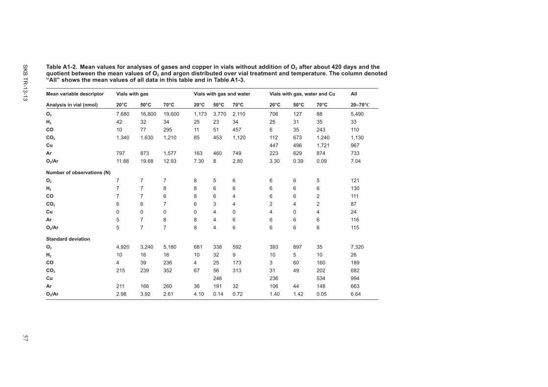
SK

B TR

-13-13 57

Table A1-2. Mean values for analyses of gases and copper in vials without addition of O2 after about 420 days and the quotient between the mean values of O2 and argon distributed over vial treatment and temperature. The column denoted “All” shows the mean values of all data in this table and in Table A1-3.

Mean variable descriptor Vials with gas Vials with gas and water Vials with gas, water and Cu All

Analysis in vial (nmol) 20°C 50°C 70°C 20°C 50°C 70°C 20°C 50°C 70°C 20–70°C

O2 7,680 16,800 19,600 1,173 3,770 2,110 706 127 88 5,490H2 42 32 34 25 23 34 25 31 35 33CO 10 77 295 11 51 457 6 35 243 110CO2 1,340 1,630 1,210 85 453 1,120 112 673 1,240 1,130Cu 447 496 1,721 967Ar 797 873 1,577 163 460 749 223 629 874 733O2/Ar 11.88 19.68 12.93 7.30 8 2.80 3.30 0.39 0.09 7.04

Number of observations (N)O2 7 7 7 8 5 6 6 6 5 121H2 7 7 8 8 6 6 6 6 6 130CO 7 7 6 8 6 4 6 6 2 111CO2 6 6 7 6 3 4 2 4 2 87Cu 0 0 0 0 4 0 4 0 4 24Ar 5 7 8 8 4 6 6 6 6 116O2/Ar 5 7 7 8 4 6 6 6 6 115

Standard deviationO2 4,920 3,240 5,180 681 338 592 393 897 35 7,320H2 10 16 16 10 32 9 10 5 10 26CO 4 39 236 4 25 173 3 60 160 189CO2 215 239 352 67 56 313 31 49 202 682Cu 246 236 534 994Ar 211 166 260 36 191 32 106 44 148 663O2/Ar 2.98 3.92 2.61 4.10 0.14 0.72 1.40 1.42 0.05 6.64

58 S

KB

TR-13-13

Table A1-3. Mean values for analyses of gases and copper in vials with addition of O2 after about 420 days and the quotient between the mean values of O2 and argon distributed over vial treatment and temperature. The column denoted “All” shows the mean values of all data in this table and in Table A1-3. Vials with gas were added with 1,600 nmol O2 at day 0. Vials with gas and water and with copper were added with 300 nmol O2 at day 0.

Mean variable descriptor Vials with gas Vials with gas and water Vials with gas, water and Cu All

Analysis in vial (nmol) 20°C 50°C 70°C 20°C 50°C 70°C 20°C 50°C 70°C 20–70°C

O2 2,134 15,000 20,800 1,030 3,460 1,810 165 637 170 5,490H2 712 33 44 27 26 37 17 21 37 34CO 12 80 328 10 62 477 7 34 258 130CO2 2,110 2,000 1,400 209 650 1,270 221 725 1,200 1,130Cu 133 339 2,670 967Ar 211 823 1,640 124 398 780 125 456 771 733O2/Ar 5.21 16.49 10.14 7.95 8 2.47 1.35 1.7 0.19 7.04

Number of observations (N)O2 9 7 6 6 7 9 7 8 5 121H2 9 8 9 6 7 9 7 8 7 130CO 9 8 8 6 7 6 7 8 3 111CO2 9 8 5 4 3 6 3 6 3 87Cu 0 0 0 0 4 0 4 0 4 24Ar 1 8 8 6 6 9 7 8 6 116O2/Ar 1 8 8 6 6 9 7 8 6 115

Standard deviationO2 1,680 2,350 3,400 476 1,600 823 70 1,350 170 7,320H2 10 14 62 4 4 12 3 4 10 26CO 4 36 287 2 15 187 2 52 25 189CO2 245 484 149 43 49 194 18 140 111 682Cu 101 78 659 994Ar 116 564 24 67 153 16 69 83 663O2/Ar 7.67 6.34 2.39 3.45 1.38 0.62 2.23 0.23 6.64

SKB TR-13-13 59

Figure A1-6. Vials with gas water and copper after exposure to O2 360 days at 50°C marked O6 and 70°C marked O9. Solid line ring circles a copper stained precipitate on the glass walls of the vials. Dotted line ring circles blackish oxides on the copper rod.

Figure A1-7. The amount of copper in vials versus the amount of argon analyzed after about 420 days. The line shows the linear regression with r = 0.7539; p = 0.00008; r2 = 0.5684.

0 500 1000 1500 2000 2500

Cu in tube (nmol)

0

200

400

600

800

1000

1200

Ar i

n tu

be (n

mol

)

60 SKB TR-13-13

Figure A1-8. The amount of copper in vials versus the amount of H2 analyzed after about 420 days. The line shows the linear regression with r = 0.8344; p = 0.000001.

Figure A1-9. The amount of copper in vials analyzed after about 420 days versus the amount of H2 analyzed after about 30 days. The line shows the linear regression H2 = 0.307× Cu – 57.1639 ; r = 0.9588; p = 0.00001.

0 500 1000 1500 2000 2500

Cu in tube (nmol)

10

20

30

40

50H

2 in

tube

(nm

ol)

0 500 1000 1500 2000 2500

Cu in tube (nmol)

0

100

200

300

400

500

600

700

800

H2 i

n tu

be (n

mol

)

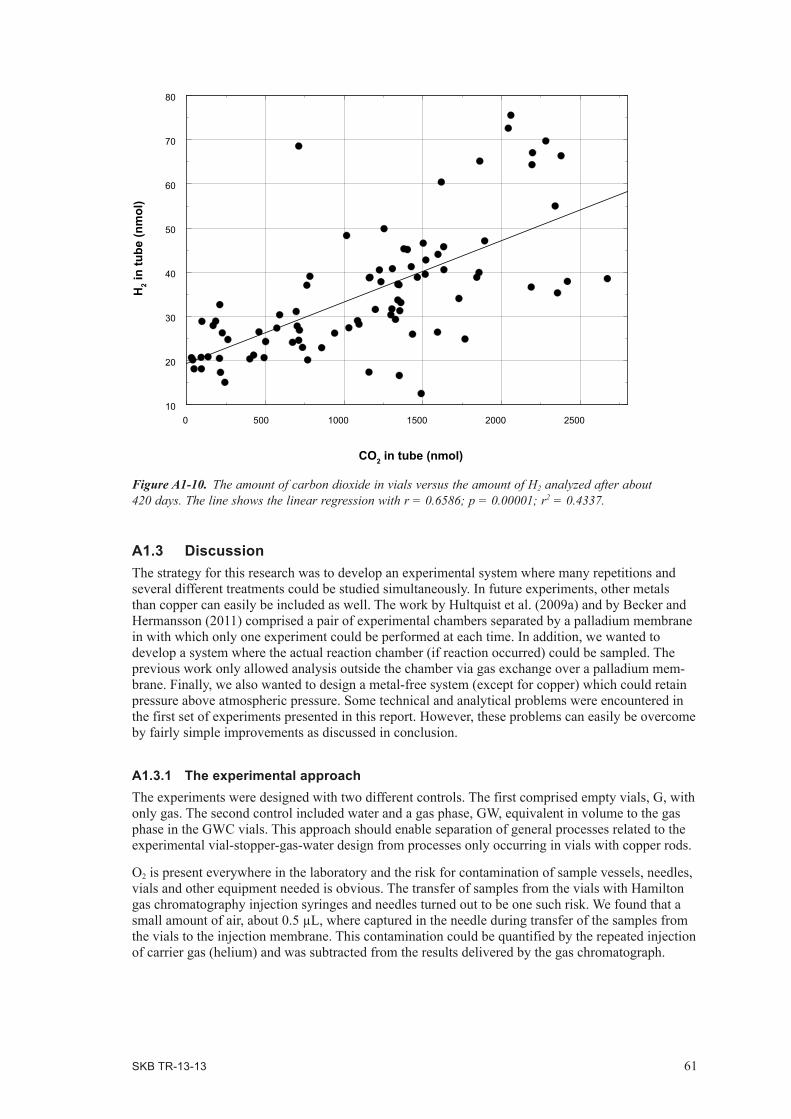
SKB TR-13-13 61

A1.3 DiscussionThe strategy for this research was to develop an experimental system where many repetitions and several different treatments could be studied simultaneously. In future experiments, other metals than copper can easily be included as well. The work by Hultquist et al. (2009a) and by Becker and Hermansson (2011) comprised a pair of experimental chambers separated by a palladium membrane in with which only one experiment could be performed at each time. In addition, we wanted to develop a system where the actual reaction chamber (if reaction occurred) could be sampled. The previous work only allowed analysis outside the chamber via gas exchange over a palladium mem-brane. Finally, we also wanted to design a metal-free system (except for copper) which could retain pressure above atmospheric pressure. Some technical and analytical problems were encountered in the first set of experiments presented in this report. However, these problems can easily be overcome by fairly simple improvements as discussed in conclusion.

A1.3.1 The experimental approachThe experiments were designed with two different controls. The first comprised empty vials, G, with only gas. The second control included water and a gas phase, GW, equivalent in volume to the gas phase in the GWC vials. This approach should enable separation of general processes related to the experimental vial-stopper-gas-water design from processes only occurring in vials with copper rods.

O2 is present everywhere in the laboratory and the risk for contamination of sample vessels, needles, vials and other equipment needed is obvious. The transfer of samples from the vials with Hamilton gas chromatography injection syringes and needles turned out to be one such risk. We found that a small amount of air, about 0.5 µL, where captured in the needle during transfer of the samples from the vials to the injection membrane. This contamination could be quantified by the repeated injection of carrier gas (helium) and was subtracted from the results delivered by the gas chromatograph.

Figure A1-10. The amount of carbon dioxide in vials versus the amount of H2 analyzed after about 420 days. The line shows the linear regression with r = 0.6586; p = 0.00001; r2 = 0.4337.

0 500 1000 1500 2000 250010

20

30

40

50

60

70

80

H2 i

n tu

be (n

mol

)

CO2 in tube (nmol)

62 SKB TR-13-13

The reason behind the erratic appearance of some of the analytic results with respect to O2 is probably the problems encountered with a batch of bad quality needles to the Hamilton syringes. Although many of the vials that had 420 or 2,200 nmol O2 added (Table A1-1) also had higher content of O2 in the analyses, it was not fully consistent and some unexplained variability was found (Figure A1-3).

Glass vials with butyl rubber stoppers have successfully been used for decades by the scientific community for cultivation of strict anaerobic microorganisms (e.g., Pedersen et al. 2008). The butyl rubber stopper has excellent properties for this purpose (Hungate et al. 1966). The use of only borosilicate glass ensured a metal free system and excluded the possibility of H2 formation from anaerobic corrosion of other metals than copper. There was a possibility that the stoppers would be contaminated with O2 (De Brabandere et al. 2012). Therefore, they were autoclaved and stored in an anaerobic O2 free box with <3.5 % H2, <5 % carbon dioxide and balance N2 for a week. Of course, then there was a risk for some contamination of the stopper with H2 and carbon dioxide.

A1.3.2 Diffusion calculations for gases through stoppers It became obvious from the obtained results and from recent literature (De Brabandere et al. 2012) that O2 was transported through the stopper into the vials (Figure A1-3 top) and it appeared as if H2 did escape the GWC 70°C vials through the stoppers (Figure A1-4 bottom). Theoretical calculations of gas transport over the butyl rubber stoppers were performed to evaluate if the observed transport rates related to literature data.

Computing the amount of O2 intruding into a test vial sealed with butylene rubber septumThe butyl rubber septa were autoclaved at 121°C and thereafter stored in an anaerobic box for at least a week to remove O2 from the stoppers. It is not clear is all O2 was removed. Here, we calculate two diffusion cases, one case with stoppers full with O2 and one case with empty stoppers. The true amount was somewhere between these numbers.

The combined gas law was first used for air outside G vials at Standard Ambient Temperature and Pressure conditions (SATP) where

P × V = n × R × T (eq. A1-1)P = Pressure (Pa)V = Volume (m3)n = Amount of gas (mol) R = gas constant = 8.31 J/mol, Kn/V = P / (R × T) = 0.21×105 / (8.31 × 298) = 8.48 mol m–3

Hence, there were 8.48 mol O2 m–3 in the air outside the stoppers of the vials during the experiment. This can be combined with knowledge of the solubility of O2 in butyl rubber at 25°C that has been determined to be approximately 0.122 m3 m–3 (Van Amerongen 1946, Brandrup et al. 1999, De Brabandere et al. 2012). This gives that the concentration of O2 in the outside surface layer of a septum was 8.48 × 0.122 = 1.03 mol m–3 during the experiment.

Now that the O2 concentrations on the outside and inside of the stopper are known (the inside is approximated to zero) the diffusion of O2 through a butyl rubber septum (the radius was 7 mm and thickness was 14 mm) can be computed using Fick’s law:

m’ = ΔC × D × A / d (eq. A1-2)m’ = mass transport (mol s–1)ΔC = concentration difference over the septum (mol m–3)D = Diffusion coefficient for O2 through butyl rubber at 25°C = 8.1×10–12 m2 s–1 (Van Amerongen 1946, Brandrup et al. 1999, De Brabandere et al. 2012)A = Septum area perpendicular to the direction of the diffusion (m2)

SKB TR-13-13 63

d = Distance the O2 must diffuse (m)m’ = (1.03–0) × 8.1×10–12 × 0.0072 × π / 0.014 = 9.2×10–14 mol s–1= 8 nmol day–1

Thus, at steady state (and 25°C) the inflow of O2 was 8 nmol day–1. We then computed the duration of steady state for a deoxygenated stopper by subtracting the duration of the experiment with the lag time before steady state was reached. This was given by:

θ = d2 / 6 × D (eq. A1-3)θ = Lag time (s) (Van Amerongen 1946, Brandrup et al. 1999, De Brabandere et al. 2012).θ = 0.0142 / 6 × 8.1×10–12 = 4.03×106 s = 46.7 days

The duration of steady state for G vials that was analyzed for O2 after 420 days was about 420–47 = 373 days.

373 days × 8 nmol day–1= 2,984 nmol

Consequently, about 3,000 nmol of O2 diffused into the test vial at 25°C. This holds true if the septum was completely deoxygenized at the start of the experiment. If the septum was fully saturated at the start of the experiment, then half the amount of O2 that the septum can hold must be added. (Half because at steady state the septum is half saturated.) This is the amount of O2 that was transferred from the septum to the test vial before steady state was reached.

From above, we know that the septum can hold 1.03 mol O2 m–3 when charged in air at SATP.

The septum volume was = 0.0072 × π × 0.014 = 2.16×10–6 m3

2.16×10–6 m3 × 1.03 mol O2 m–3 = 2,225 nmol2,984 nmol + 2,225 / 2 nmol = 4,097 nmol

Consequently, if the septum was saturated at the start of the experiment then about 4,100 nmol O2 diffused into the test vial during the experiment.

The calculations for the case where the temperature was 70°C are very similar to those above. The difference is that the diffusivity and solubility of O2 in butyl rubber at 70°C must be known. They are not explicitly given by the cited literature (Van Amerongen 1946, Brandrup et al. 1999, De Brabandere et al. 2012) but the expressions (eq. A1-4) and (eq. A1-5) below were given.

D = D0 × exp(–Ed / (R × T)) (eq. A1-4)D0 = Computed from data at 25°C and is 4.39×10–3 m2/sEd = Activation energy for diffusion = 49.8 kJ/mol

S = S0 exp(–Es / (R × T)) (eq. A1-5)S0 = Computed from data at 25°C and is 16.16×10–3 Es = Heat of solution = –5 kJ/mol

S0 is a constant in the thermal dependency equation of S (from Brandrup et al. 1999).

In addition to account for faster diffusion at higher temperature, the increasing concentration of O2 in the vials during the experiment must be taken into account. Approximating the concentration in the vials to zero does not give the correct answer when the temperature is 70°C because the concentra-tion soon becomes significantly above zero. If the same calculations as was done for 25°C are used the concentration of O2 in the test vials rises to about 18 % of the concentration on the outside. This means that the concentration in the test vials has been 9 % on average during the experiment. Steady state is reached after 3.3 days at 70°C so it is a good approximation to use the same calculations as in the 25°C case and subtract 9% in the end. This gives the results 26,091 nmol and 25,475 nmol for O2 saturated and deoxygenized septa, plus the 7.4 × 60 = 444 nmol that entered the vials between days 360 when the vials were cooled to room temperature and 420 days when the last analyses were performed.

64 SKB TR-13-13

Calculation of amount of H2 escaping from test vial sealed with butylene rubber septumAs in the case with O2, Fick’s law (eq. A1-2) is used in the calculations. The volume of the vials did not change during the experiment. This means that mass transport is essentially the same thing as concentration change and one way of interpreting Fick’s law is to state that “The rate of concentra-tion change is dependent on the level of concentration multiplied by something else that does not change with time.” Fick’s law can be re-written on differential form as (eq. A1-7) with the use of the trivial (eq. A1-6) below. This is a commonly used, and well known, differential equation that reoccurs in several forms in many branches of the natural sciences (for example discharge of electric capacitor and biomass growth).

m = C × V (eq. A1-6)m = amount (mol)C = concentration (mol m–3)V = Volume (m3)

∂C/∂t = –C × P × A / (d ×V) (eq. A1-7)P = Permeability

The solution to this equation is:

C = C0 × e–P × A × t / (d × V) (eq. A1-8)t = time (s)C0 = concentration at t=0

Using (eq. A1-8), it is possible to directly compute the concentration in a test vial at any given time (for example 420 days) provided that the concentration at t = 0 is known. Another use of (eq. A1-4) is that it is easily used to compute the quotient between the concentrations at two different times (for example t = 420 and t = 0 days).

At 25°C: Ct=420 days / Ct=0 = e–k / 1 = [k = –5.3a × 10–12 × 0.0072 × π × 420 × 86,400 / (0.014 × 25 × 10–6)] = 0.655 a (Data from Brandrup et al. 1999)

This means that during the experiment about 35 % of the original H2 escaped if the temperature was 25°C.

At 70°C: Ct=420 days / Ct=0 = e–k / 1 = [k = –5.3b × 10–11 × 0.0072 × π × 360 × 86,400 / (0.014 × 5 × 10–6 )] = 0.027b Assuming that the permeability for H2 is 10 times higher at 70°C than at 25°C.

This assumption is supported by the fact that the permeability of O2 through butyl rubber at 25°C and 70°C is 10.8 according to De Brabandere et al. (2012) and that the quotes for 15 other rubber compounds were all around 10 according to Brandrup et al. (1999). In addition, Figure 77-01 by Massey (2003) supports this assumption. That graph concerned N2 diffusing through butyl rubber but there is no reason to assume that the H2 temperature dependence is substantially different from that of O2 and N2, whose temperature dependencies are similar to each other.

This means that during the experiment about 97 % of the original H2 escaped if the temperature was 70°C.

A1.3.3 The gas filled vialsThe observed increase in O2 in the G vials followed the theoretical calculations above very well. There was a decrease in O2 in the vials after 30 days, compared to the added amount, of about 1,000 nmol, most obvious in the O-series vials (Figure A1-3 top). This is consistent with deoxygenated stoppers that would adsorb about 1,100 nmol of O2 before the diffusion of O2 from the outside would have turned the O2 transport back into the vials (A1.3.2). Similarly, there was an increase in H2 of about

SKB TR-13-13 65

40–50 nmol to a total of at most 60 nmol of which most probably came from the stoppers that was stored in a 2–3 % H2 environment for at least a week (Figure A1-4). In opposite to O2, the amount of H2 decreased after day 30 and reached an average of about 40 nmol after 420 days which is very close to the 35 % decrease predicted by the diffusion calculations (A1.3.2).

O2 continued to increase over time and was on average 4,000 nmol after 420 days in 20°C (Figure A1-3), again close to the predicted value range between 3,000 and 4,000 nmol depending on how well the stoppers were deoxygenated. At 70°C, the calculations predicted about 26,000 nmol and about 20,000 nmol were observed. Possibly, the counter outgoing diffusion effect from increasing O2 concentrations inside the vials may have slowed the increase in O2 more than predicted. In addition, the diffusion parameters for the stoppers used here may differ from the literature parameters obtained for the calculations. More important than obtaining exact numbers is that the results clearly show that O2 was transported to the inside of the vial as a function of time. In opposite, H2 did not increase after 30 days – that gas decreased in all G vials over time which in line with an initial pulse of H2 from the stopper (from the anaerobic box) to the inside of the vial; a transport that later was reversed resulting in H2 leaving the vials. In other words, there was no emission of H2 in N2 filled G vials.

Argon increased as a function of temperature (Table A1-2 and Table A1-3) which further attests an inflow of O2 from air accompanied by argon that is also present in air (0.93 %). The amount of carbon dioxide was similar in all three temperatures in the G vials (Table A1-2 and Table A1-3) which suggests that this gas mainly came from the stoppers just like H2 did. Carbon dioxide was present in the anaerobic box gas environment as well.

Finally, the amount of carbon monoxide increased exponentially after day 30 and the increase was positively correlated with temperature. There was no difference between N and O series vials. These results suggest either transport of carbon monoxide from the outside into the vials, or, that the stop-pers degraded under the generation of carbon monoxide as a function of temperature. The highest amount observed was about 500 nmol per vial which is equivalent to about 20 µmol carbon dioxide per Litre of gas, or 480 µL L–1, which is far higher than what is found indoor in air where at most a few µL L–1 can be found. Consequently, it remains to explain the occurrence of growing amounts of carbon monoxide in the vials as some kind of stopper induced effect. This process needs further exploration before the causes behind such a process can be conclusively determined.

A1.3.4 The vials with gas and waterThe GW vials differed from the G vials in that about 21 mL of the total volume of 26 mL in the vials were replaced with water. The volume of the gas phase in GW vials was consequently about 20% of that in the G vials meaning that the concentration of gases, i.e. O2, diffusing inwards increased 5 times faster in the GW vials compared to what it did in the G vials. Further, with water in the vials, the solubility of the head space gases in water should be considered. Finally, the stoppers were in contact with water at the bi-monthly mixing occasions and there was water vapour in the headspace that must have increased in concentration with increasing temperature.

Henry’s law states that at a constant temperature, the amount of a given gas that dissolves in a given type and volume of liquid is directly proportional to the partial pressure of that gas in equilibrium with that liquid. In other words, the solubility of O2, H2 and other vial gases in the vial water was proportional to the pressure of each of the gases in the head space as a function of temperature.

Some Henry’s constants for the distribution of gases are given and defined in Table A1-4. These numbers can be used to calculate the amount of dissolved gases in the vials as:

Caq = kH,cc × Cgas (eq. A1-9)

The GW vials had at most 4,000 nmol / 5 mL = 800 nmol O2 mL–1 gas in the headspace at day 360. There were 21 mL of water in the GW vials. The amount of dissolved gas in the water was then = 3.181 × 10−2 × 800 × 21= 534 nmol or 25 nmol O2 mL–1. This shows that close to 90 % of the O2 in the vials was allocated to the headspace. The solubility of gases in water generally decreases with increasing temperature. The ratio of O2 in headspace to water would then have increased at the higher temperatures 50°C and 70°C. A similar reasoning can be held for all other gases in the vials.

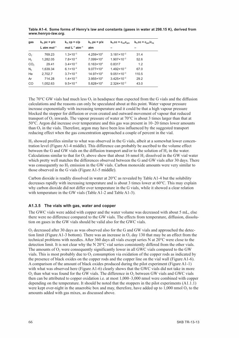
66 SKB TR-13-13

The 70°C GW vials had much less O2 in headspace than expected from the G vials and the diffusion calculations and the reasons can only be speculated about at this point. Water vapour pressure increase exponentially with increasing temperature and it could be that a high vapour pressure blocked the stopper for diffusion or even created and outward movement of vapour that reduced transport of O2 inwards. The vapour pressure of water at 70°C is about 3 times larger than that at 50°C. Argon did increase over temperature and this gas was present in 10–20 times lower amounts than O2 in the vials. Therefore, argon may have been less influenced by the suggested transport reducing effect when the gas concentration approached a couple of percent in the vial.

H2 showed profiles similar to what was observed in the G vials, albeit at a somewhat lower concen-tration level (Figure A1-4 middle). This difference can probably be ascribed to the volume effect between the G and GW vials on the diffusion transport and/or to the solution of H2 in the water. Calculations similar to that for O2 above show that about 16 nmol H2 dissolved in the GW vial water which pretty well matches the differences observed between the G and GW vials after 30 days. There was consequently no H2 emission in the GW vials. Carbon monoxide amounts were very similar to those observed in the G vials (Figure A1-5 middle).

Carbon dioxide is readily dissolved in water at 20°C as revealed by Table A1-4 but the solubility decreases rapidly with increasing temperature and is about 3 times lower at 60°C. This may explain why carbon dioxide did not differ over temperature in the G vials, while it showed a clear relation with temperature in the GW vials (Table A1-2 and Table A1-3).

A1.3.5 The vials with gas, water and copperThe GWC vials were added with copper and the water volume was decreased with about 5 mL, else there were no difference compared to the GW vials. The effects from temperature, diffusion, dissolu-tion on gases in the GW vials should be valid also for the GWC vials.

O2 decreased after 30 days as was observed also for the G and GW vials and approached the detec-tion limit (Figure A1-3 bottom). There was an increase in O2 day 130 that may be an effect from the technical problems with needles. After 360 days all vials except series N at 20°C were close to the detection limit. It is not clear why the N 20°C vial series consistently differed from the other vials. The amounts of O2 were consequently significantly lower in all GWC vials compared to the GW vials. This is most probably due to O2 consumption via oxidation of the copper rods as indicated by the presence of black oxides on the copper rods and the copper line on the vial wall (Figure A1-6). A comparison of the amount of black oxides produced during the pilot experiment (Figure A1-1) with what was observed here (Figure A1-6) clearly shows that the GWC vials did not take in more O2 than what was found for the GW vials. The difference in O2 between GW vials and GWC vials then can be attributed to copper oxidation i.e. at most 1,000–3,000 nmol were combined with copper depending on the temperature. It should be noted that the stoppers in the pilot experiments (A1.1.1) were kept over-night in the anaerobic box and may, therefore, have added up to 1,000 nmol O2 to the amounts added with gas mixes, as discussed above.

Table A1-4. Some forms of Henry’s law and constants (gases in water at 298.15 K), derived from www.henrys-law.org.

gas kH, pc = p/c kH, cp = c/p kH, px = p/x kH,cc = caq/cgas kH,cc = cgas/caq

L atm mol–1 mol L–1 atm–1 atm – –

O2 769.23 1.3×10−3 4.259×104 3.181×10−2 31.4H2 1,282.05 7.8×10−4 7.099×104 1.907×10−2 52.6CO2 29.41 3.4×10−2 0.163×104 0.8317 1.2N2 1,639.34 6.1×10−4 9.077×104 1.492×10−2 67.0He 2,702.7 3.7×10−4 14.97×104 9.051×10−3 110.5Ar 714.28 1.4×10−3 3.955×104 3.425×10−2 29.2CO 1,052.63 9.5×10−4 5.828×104 2.324×10−2 43.0

SKB TR-13-13 67

The amount of H2 in the 20°C and 50°C vials were similar to what was observed in the GW vials. At 70°C there was a significant H2 emission after 30 days that reached values about 100 times higher than in all other vial treatments. After 30 days the H2 amount decreased to less than 5 % of the maximum values. Average maximum value in the O series was 717 nmol H2 and average after 360–420 days was 36 nmol H2. This decrease is explained by the outward diffusion of H2 that was calculated to be about 3 %. The difference between 5 % and 3 % can be due to differences in butyl rubber stopper composition compared to the rubber used to generate the literature data. It could also be that there was some residual H2 emission going on after 30 days that compensated for a small part of the outward transport.

There was no clear difference in H2 emission between the O and N series. There was a drop in O2 amount in both the O and N series vials after 30 days concomitant with the peak in H2. Unfortunately, it is difficult to resolve if the 70°C vials were totally O2 free or not during the most intensive H2 emission that took place the first 30 days. It can be argued that there indeed was O2 present in the O series and that H2 was emitted in these vials to amounts similar to what found in the N series. This then suggests that H2 was emitted in presence O2. However, given the oxygen sorption effect of the stopper that was present in both the O and N series vials and the low amount of O2 that dissolved in water at 70°C i.e. less than 5 % of what was left in the headspace after 30 days (< 400 nmol Figure A1-3 bottom), the aqueous environment in the both the O and N series GWC vials may have been very close to O2 free with at most a few nmol O2 mL–1. After 30 days, inward diffusion of O2 once the stopper was saturated from the outside may have started to raise the amount of O2 in the water to levels where H2 emission stops. Although this is a rather speculative approach, it would explain why there was no H2 emission in the 20°C and 50°C GWC vials. There the vapour pressure was three times lower than in the 70°C GWC vials which possibly allowed for a more rapid inward transport of O2 that oxygenated the environment, as discussed above. In addition, the solubility of O2 was about 40 % lower at 70°C than at 50°C which would contribute to nearly anoxic conditions in the 70°C GWC vials. This speculation would imply that the low amounts of O2 in the 20°C and 50°C GWC vials was due to consumption of O2 by the copper in these vials producing a blackish precipitate, a process that was absent in the 70°C GWC vials due to the assumed absence of O2 in the water. Admittedly a bit farfetched explanation at this stage, but it would be worth testing in new experiments.

The amount of copper in the vials after removal of the copper rods correlated with the amount of H2 analyzed after 30 day (Figure A1-8) and also with H2 analyzed after 420 days (Figure A1-7) in the 70°C GWC vials. This correlation indicated a relation between H2 emission and a copper corrosion process that liberated copper from the test surfaces. On a molar basis there were about three copper atoms in solution per H2 molecule. This ratio is in the regime of what could be explained by the reaction suggested by Hultquist et al. (2011).

Cu (s) + H2O (aq) ↔ CuOH (s) + ½ H2 (g) (eq. A1-10)

There may also have been an aerobic corrosion process after 30 days that released copper from the surfaces to solution which would explain the detected copper not covered by reaction 10. Further, it is also possible that the total amount of produced H2 was higher than analyzed due to the outward diffusion of this gas.

The observed partial pressure was 2–3 times larger (A1.2.2) than what was reported previously (1 mbar) (2011). Here, we analyzed H2 inside the “reaction chamber” at about 200 kPa pressure while the previous experiments were analyzed outside a palladium membrane at low pressure. The discrepancy in calculated/observed partial pressure may then relate to from where the H2 was analyzed and differences in the used analytical instruments.

The conclusive answer to if H2 emitted according to reaction A1-10 requires a second experimental series where the control of O2 is improved and shorter experimental times may also be required. It is fairly simple to set the experimental conditions to fulfil this requirement as presented in conclusion.

68 SKB TR-13-13

A1.3.6 Water gas shift reactionThe water-gas shift reaction (Ladebeck and Wagner 2003) would produce H2 if carbon monoxide and water were present, as was the case here.

CO + H2O ↔ CO2 + H2 (eq. A1-11)

However, there was no difference in the amounts of carbon monoxide between G, GW and GWC vials after 30 days (Figure A1-5) and the actual amounts was less than 5 nmol which is far too little to explain the observed emission of 500–700 nmol H2. The observed correlation between H2 and carbon dioxide (Figure A1-10) was related to lower solubility of carbon dioxide with increasing temperature as reflected by Table A1-2 and Table A1-3, which in turn was related to the amount of H2 produced in the 70°C GWC vials and not to a water-gas shift reaction.

A1.3.7 Conclusion and improvementsIn line with what has been described elsewhere (Becker and Hermansson 2011, Hultquist et al. 2011) emission of H2 in pure anoxic water was indicated. The experimental conditions need some improve-ments before conclusive results can be obtained.

1. Stoppers for anaerobic experiments must be stored in pure N2 which easily can be achieved using anaerobic chambers with a N2 environment and not in the anaerobic box with traces of H2 and carbon dioxide as was done here.

2. Stoppers for O2 doped experiments must be stored in air to charge them with O2 and avoid the O2 suction effect of the stoppers found in this work. Ideally, it should be the same gas mixture as used for experiments.

3. Vials must be incubated in a shielded N2 environment and not in air as was done in the reported experiments.

4. Analyses should be performed with shorter time intervals in the 7–14 days regime because the observed process obviously was rapid.

5. The injection technique on the chromatographs must be added with a carrier gas stream over the injection septa.

6. Obviously, syringes and needles must be of good quality.

SKB TR-13-13 69

Appendix 2

Development Phase IIA first series of vials with copper in water were set in spring 2010 and followed for about 420 days. These experiments are referred to whenever appropriate as Development Phase I experiments.

A2.1 Upgraded experimental methodAll the six suggestions for method improvements from Development Phase I (A1.3.7) were dealt with as follows:

1. Stoppers for all experiments were stored in anaerobic jars with a N2 atmosphere.

2. Experiments with O2 were not performed.

3. Vials were incubated in anaerobic jars with a N2 atmosphere.

4. Analyses were generally performed with 10 to 20 days’ time interval because the observed H2 emission process was previously indicated to be rapid in Development Phase I.

5. The injection technique on the chromatographs was upgraded and a new chromatograph (Bruker 450) with a Pulsed Discharge Helium Ionization Detector (PDHID) was employed for the H2 and O2 analyses.

6. Syringes and needles were of good quality.

H2 was analyzed on the Bruker 450 chromatograph with PDHID. This system was new when the experiments started. It was found equally sensitive for H2 compared to the KAPPA V used during 2010.

Further, we changed the vial production procedure from a one by one production to a 10 by 10 vials production. This procedure enabled a more time efficient process with a good vial environment quality.

A2.2 Materials and MethodsA2.2.1 ExperimentsThree experiments were performed to further study the emission of H2 from copper in water. In the first test, we analyzed H2 from copper in water at 70°C with two different copper rod treatments. The second experiment reproduced the experiment from Development Phase I without O2 treatments at the temperatures 30°C, 50°C and 70°C. The third experiment tested an alternative surface treat-ment with exposure to 50°C over night under anoxic conditions prior to immersion of the copper rods in water.

A2.2.2 Experiment overviewThe present experimental set-up was generally configured as done in Development Phase I (Table A1-1). The experiments were designed to evaluate the extent of H2 emission in compartments containing water-immersed copper under anoxic conditions. Accordingly, copper rods were thoroughly washed and completely immersed in O2-free water. Vials were incubated in darkness at three temperatures – at 30°C, 50°C or 70°C or at one temperature only, 70°C. Analyses of the vial atmosphere H2 contents were performed at up to 6 sample occasions – at experiment start (S1) up to at most 90 days after start (Table A1-1). Variations in the vial production relative to the procedure applied in Development Phase I are given under respective experiment.

70 SKB TR-13-13

Table A2-1. Experimental overview. Each experiment hosted one or three types of vials: gas-only negative controls denoted ‘G’, water-filled negative controls denoted ‘GW’ and water-submerged copper-containing experimental vials denoted ‘GWC’.

Experiment Series Vial content

No of vials

°C Incubation Time (days) Approximate Gas Volume (mL)S1 S2 S3 S4 S5 S6

1 B1 GWC 5 70 0 9 20 29 60 – 6.21 B2 GWC 5 70 0 9 20 29 60 – 6.22 N1 G 5 30 0 12 30 42 55 90 26.22 N2 GW 5 30 0 12 30 42 55 90 10.22 N3 GWC 10 30 0 12 30 42 55 – 6.22 N4 G 5 50 0 12 30 42 55 90 26.22 N5 GW 5 50 0 12 30 42 55 90 10.22 N6 GWC 10 50 0 12 30 42 55 – 6.22 N7 G 5 70 0 12 30 42 55 90 26.22 N8 GW 5 70 0 12 30 42 55 90 10.22 N9 GWC 10 70 0 12 30 42 55 – 6.23 N20 G 5 70 0 10 24 38 – – 26.23 N21 GW 5 70 0 10 24 38 – – 6.23 N22 GWC 10 70 0 10 24 38 – – 6.2

A2.2.3 Experimental preparations of copper rodsCopper rods measuring 100×10×2 mm, exhibiting a 15 degree angle at one end were machine cut from O2-free, phosphorus doped copper (Cu-OFP) and engraved with running numbers (Figure A1-2). Copper rods had previously been used in Development Phase I and had obtained significant oxide layers. Therefore, all surfaces were thoroughly hand grinded with fine grained abrasive paper to obtain metallic copper rods, washed thoroughly with detergent under hot water, dried with paper and immediately transferred into in an anaerobic glove box environment (COY Laboratory Products, MI, USA) and stored until experiment start, immersed in 99% ethanol in a closed vessel.

All solutions used during preparations were sterilized in autoclave at 121°C for 15 minutes and, where applicable, prepared using Millipore Direct-Q purified water. In addition, all solutions used were gassed prior to use by thorough bubbling with N2 directly after sterilization. All handling was performed using clean gloves and tweezers.

26 mL gas tight, anaerobic borosilicate experimental vials (Product #2048-18150, Bellco Glass Inc., NJ, USA) and matching impermeable butyl rubber stoppers (Product #2048-117800) were used. These stoppers were immersed in water, autoclaved at 121°C for 20 minutes and placed under sterile conditions over at least 7 days in an anaerobic jar with N2 atmosphere. In the anaerobic box, copper rods were withdrawn from storage, placed in >70% ethanol in sonicator bath and incubated for 5 minutes to remove surface contaminants. Rods were extracted from the sonicator bath and washed twice sequentially in 250 mL water and placed in a 50 g L–1 acid bath during 10 minutes to remove any corrosion products present on copper rod surfaces according to ISO 8407:2009 – Corrosion of metals and alloys – Removal of corrosion products from corrosion test specimens. Remaining acid from the acid bath was allowed to drain from the copper rods during a one-minute incubation on lint-free paper. Subsequently, copper rods were washed four times sequentially in 100 mL Millipore Direct-Q water, allowed to dry on lint-free paper and then placed pair wise in antiparallel orientation in the experimental vials.

Following positioning of copper rods, experimental vials were sealed using butyl rubber stoppers without coating. Sealed vials were capped with an aluminium ring and transferred from the anaero-bic box for evacuation and water application. Exact inner volume of capped, sealed experimental vials was approximately 26.2 mL.

SKB TR-13-13 71

Sealed vials were removed from the anaerobic glove box and immediately evacuated six times down to at least 2.0 kPa. Vials were filled with about 120 kPa Instrument N2 between evacuations. Following the sixth evacuation, vials were left at 1.2 kPa. Vials targeted for gas-only filling were filled with Instrument N2 to a total pressure of about 150 or 200 kPa. Vials targeted for water nega-tive controls and copper containing experimental vials were weighed, filled with about 21 or 17 mL autoclave sterilized, anoxic Millipore Direct-Q water that had been purged with N2 for 1 hour (Butler et al. 1994) and then weighed again, in order to procure the exact amount of water added (and thus the exact remaining gas volume). All fillings were made using thoroughly sterilized and N2-rinsed equipment and gas lines.

Immediately following water additions, vials were again immediately evacuated six times down to at least 2.0 kPa and boiling of the water was allowed for about 30 seconds. Final pressure was set to 150 kPa.

A2.2.4 Gas analysesGas sampling and analyses were initiated by allowing all vials to cool to room temperature. All vials, needles and equipment used were thoroughly flushed with Scientific He prior to attachment or insertion into experimental or control vials. All sampling was performed using an identical method. A Bruker 450 gas chromatograph equipped with a CP7355 PoraBOND Q 50m x 0.53mm ID and a CP7536 MOLSIEVE 5A PLOT 25m x 0.32mm ID and a Pulsed Discharge Helium Ionization Detector (PDHID) was employed for the H2 analyses (Bruker Daltonics Scandinavia AB, Vallgatan 5, SE-17067 Solna, Sweden). First, a needle attached to a pressure gauge was inserted into the gas volume and the initial pressure was noted. Second, a 100 µL sample was extracted and immediately injected into the GC-injector of the Bruker 450 chromatograph for H2 analysis. H2 concentrations above the detection range for the 450 GC were performed on a Varian 3400CX gas chromatograph (Agilent Technologies Inc., CA, USA). The chromatographs were calibrated with a special gas mix (Linde specialgas, AGA, certificate no: 30008-1) H2, 24.6 ppm; CO 24.9 ppm; N2, 999950 ppm.

A2.2.5 O2 report levelDuring Development Phase I we found that air was captured in the syringe needle during transfer of the sample from the vial to the injector on the gas which resulted in O2 data not related to the gas phase in the vials. Therefore, at regular intervals, we started to inject carrier gas (He) for determina-tion of this the injection error. It was found that between 0.2 and 0.5 mL air i.e. between 0.04 and 0.l mL O2 were captured during injection. The exact amount depended on the skills of the respective technician and we started specific injection training during Development Phase II that became fully developed during Method validation. In several of the result figures there is an undulating trend in O2 values and sometime relatively high O2 values. We did have problems with air leakages during sampling that occasionally appeared to introduce oxygen in the vials, but it is difficult to separate the injection error from other leakages. At present, for Development Phase II results, it can be assumed that O2 was present in the vial if the results are above 40–50 nmol O2 mL–1. Values below 40–50 nmol O2 mL–1 generally reflect air capture during injection of the samples. Values above 40–50 nmol O2 mL–1 suggest that there has been a contamination of the vial gas environment due to leakages. Occasionally, the vial pressure became close to, or below atmospheric pressure during the last sample occasions. In these samples, the amount of air contamination increased significantly.

A2.2.6 Copper analysisAll vials in experiment 1 and a selection of vials from experiment 2 were sent to ALS Scandinavica AB, Luleå for analysis. The method is accredited for drinking water and the analysis protocol denoted V-2, elements in water, was applied. This method had a detection limit of 10 mg Cu L–1. Briefly, the vials from experiment 1 were opened at ALS Scandinavica AB, Luleå and the copper rods were removed and the water was acidified and analyzed. However, Postal transport broke one of the vials. Therefore, copper rods were removed in an anaerobic box from the vials, the vials were sealed again and then shipped for copper analysis.

72 SKB TR-13-13

A2.2.7 Experiment 1: 2012-04-04 – 2012-05-06This experiment was set to reproduce the H2 emission results from Development Phase I at 70°C with somewhat changed general conditions. We used Instrument instead of Scientific N2 and we used a gas bench for filling and evacuation 10 vials at the time. The copper rods were hand grinded in difference to the machine produced surfaces in Development Phase I. In this experiment specifically, five copper rods were treated as done in Development Phase I and for the five remaining surfaces, sonication in ethanol and acid cleaning was skipped.

A2.2.8 Experiment 2: 2012-05-09 – 2012-08-07This experiment reproduced the work performed in Development Phase I with the general conditions used for experiment 1. However, it soon became obvious that there was a too high background of H2 in the vials that was traced to the gas bench. The O2 scavenger of this bench is re-generated occa-sionally with H2 and a filter system trapped H2. The filter system was removed and the vials were evacuated again after day 15 (except GWC vials 70°C) that already had emitted H2 to concentrations much higher than the background. After day 25, five of the GWC vials 70°C were evacuated and filled with N2 to investigate if the H2 evolving process continued.

A2.2.9 Experiment 3: 2012-06-01 – 2012-07-12This experiment tested the influence of storage of cleaned copper rods in the vials at 50°C over night prior to filling with water, as an alternative to storage in the anaerobic box. It could ease preparation procedure if storage is possible prior to filling with water.

A2.3 Results and discussion The work presented in this report was focussed on development of a procedure to reproducibly observe emission of H2 from copper in anoxic water. Therefore, variations in the method were applied in Development Phase II relative to what was performed in Phase 1. Inherent in this approach is a risk for an increased sample result variation. However, we did have very good documentation of the different procedures applied and understand what may have caused most of this variability.

A2.3.1 CalculationsThe 450 Bruker GC was calibrated with varying volumes of H2 and O2 and the output from the GC consequently was volumes of the respective analyzed gas per injected volume of sample. This report shows gas data as nmol per vial, nmol mL–1 at atmospheric pressure or mbar of the respective ana-lyzed gas in the vial gas phase. The combined gas law was used for calculating these values where

P × V = n × R × TP = Pressure (Pa)V = Volume (m3)n = Amount of gas (mol) R = gas constant = 8.31 (J mol–1 K–1)T = Temperature (K)

The amounts of analyzed gases per volume of sample (nmol mL–1) at ambient room pressure and temperature were calculated where

n/V1 = P1 / (R × T) = (V1/V2×P2) / (R × T) = mol m–3 mol m–3 = 1,000 nmol mL–1

n = Amount of gas in sample (mol) V1 = analyzed amount of H2 or O2 in sample (m3)V2 = volume injected sample (m3)

SKB TR-13-13 73

P1 = Analyzed sample pressure (Pa)P2 = Pressure in analysis room (Pa)R = gas constant (J mol–1 K–1)T = Temperature in analysis room (K)

Second, the total amounts of the analyzed gases in the vial (nmol per vial) were calculated where

nmol in vial = nmol mL–1 × V3 × P3 V3 = Volume gas in vial (m3)P3 = Pressure in vial after sampling (Pa)

Finally, the partial pressures (mBar) of the analyzed gases in the vial were calculated using Dalton’s law of partial pressures where

P4 /P3 = V1/V2

P4 = V1/V2 × P3

P4 = Partial pressure of analyzed gas in vial (Pa)

Recalculating Pa to bar

P4/100,000 = P5

P5 = Partial pressure of analyzed gas in vial (bar)

A2.3.2 Experiment 1Acid cleaned copper rods produced an average (n=5) of 1.5 mbar H2 per vial after 20 days (Figure A2-1). Non-acid cleaned surfaces, on the other hand, produced only approximately 0.5 mbar H2 per vial after 20 days. Eventually, non-acid cleaned vials produced an average of 1.5 mbar H2 per vial after 64 days. There was a large diversity in the data and individual vials produced very different amount of H2. Partly, this was due to pressure drops in the vials, possibly caused during penetration for sam-pling and pressure measurement. Three vials appeared to have inactive copper rods that produced no H2 compared to the start values. The observed average of approximately 1.5 mbar (500 nmol) H2 per vial corresponds well with what was observed for a similar experimental series during Development Phase I (c.f. Figure A1-4).

A2.3.3 Experiment 2In this experiment we encountered some problems with a high background of O2 and H2 in the vials caused by a technical problem with our gas bench as described in the methods section (A2.2.4). The analysis of O2 on the Bruker 450 GC was under development and there is, therefore, some uncertainty connected with the O2 values, i.e. if they were due to problems with the gas bench or with the setup of O2 analysis (See A2.2.5 for details). After the modification of the gas bench we monitored the gas quality at all filling occasions and H2 was always on the detection limit of the GC 450 < 1 nmol mL–1. This is obvious from the results that show a decrease in H2, O2 and pressure after 10 days due to replacement of the gas phase in the vials (Except for series N9) to a lower total gas pressure (Figure A2-2 and Figure A1-3). We also encountered problems with pressure drops in the vials which was caused by sampling; a too rapid pulling out of needles during sampling and pres-sure measurements cased some de-gassing. The method was later, in Method validation, changed to a slower procedure that reduced this problem. The amount of H2 in this experiment is represented as partial pressure of H2 in in the vials. In the 70°C series N9, vial pressures became below atmospheric pressure and the injection error became very large (Figure A2-4). Therefore, all series N8 and N9 vials were re-pressurised with N2 after day 42 which diluted H2 and caused a drop in the partial pres-sure of H2. The results are kept in the figures for their illustrative character regarding pressure drop and O2 contamination during injection.

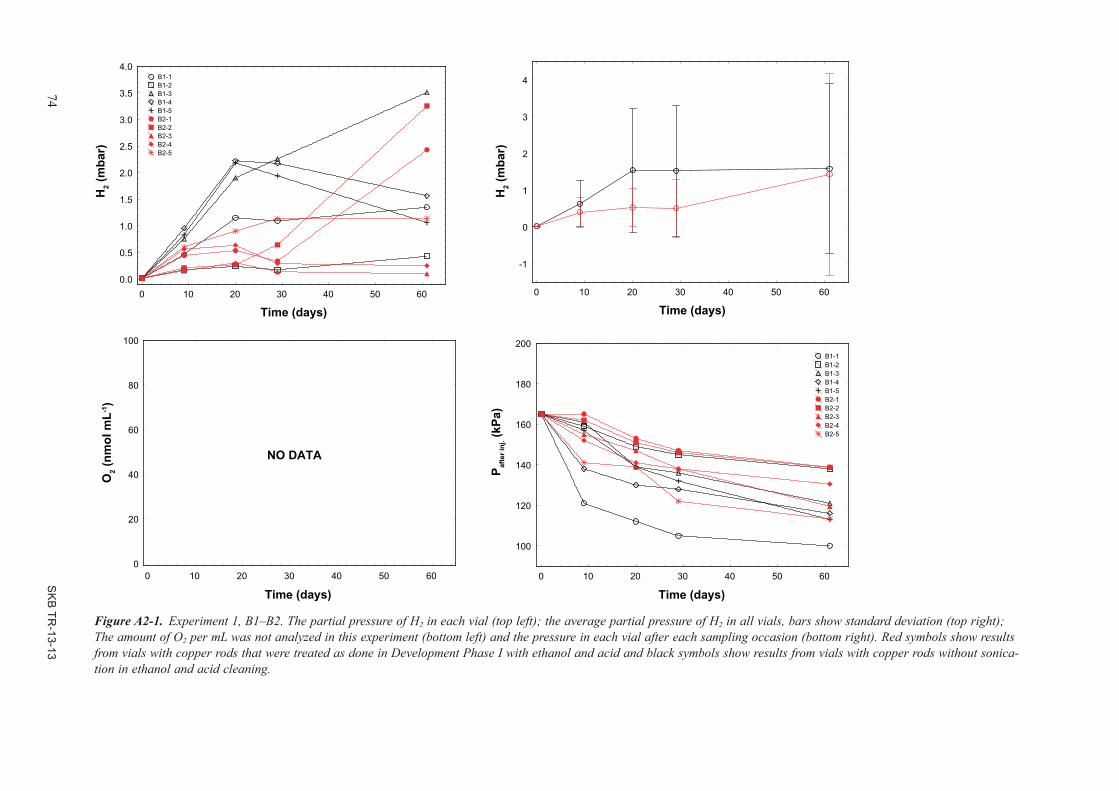
74 S

KB

TR-13-13

Figure A2-1. Experiment 1, B1–B2. The partial pressure of H2 in each vial (top left); the average partial pressure of H2 in all vials, bars show standard deviation (top right); The amount of O2 per mL was not analyzed in this experiment (bottom left) and the pressure in each vial after each sampling occasion (bottom right). Red symbols show results from vials with copper rods that were treated as done in Development Phase I with ethanol and acid and black symbols show results from vials with copper rods without sonica-tion in ethanol and acid cleaning.

0 10 20 30 40 50 60

Time (days)

-1

0

1

2

3

4

0 10 20 30 40 50 60

Time (days)

0

20

40

60

80

100

0 10 20 30 40 50 60

Time (days)

100

120

140

160

180

200 B1-1 B1-2 B1-3 B1-4 B1-5 B2-1 B2-2 B2-3 B2-4 B2-5

0 10 20 30 40 50 60

Time (days)

0.0

0.5

1.0

1.5

2.0

2.5

3.0

3.5

4.0 B1-1 B1-2 B1-3 B1-4 B1-5 B2-1 B2-2 B2-3 B2-4 B2-5

NO DATA

H2 (

mba

r)

H2 (

mba

r)

O2 (

nmol

mL-1

)

P afte

r inj

. (kP

a)

SK

B TR

-13-13 75

Figure A2-2. Experiment 2, N1–N3, 30°C. The partial pressure of H2 in each vial (top left); the average partial pressure of H2 in vials per series, bars show standard deviation (top right); the analyzed amount of O2 nmol mL–1 in each vial (bottom left), and the pressure in each vial after each sampling occasion (bottom right).black symbols: vials with gas (N1, G); red symbols: vials with gas and water (N2, GW) and blue symbols: vials with gas, water and copper.

0 10 20 30 40 50 60 70 80 90

-0.02

0.00

0.02

0.04

0.06

0.08

0.10

0.12

0.14

0.16

0.18

0.20

0 10 20 30 40 50 60 70 80 900

100

200

300

400

500

600 N1:1 N1:2 N1:3 N1:4 N1:5 N2:1 N2:2 N2:3 N2:4 N2:5 N3:1 N3:2 N3:3 N3:4 N3:5 N3:6 N3:7 N3:8 N3:9 N3:10

0 10 20 30 40 50 60 70 80 90

100

120

140

160

180

200 N1:1 N1:2 N1:3 N1:4 N1:5 N2:1 N2:2 N2:3 N2:4 N2:5 N3:1 N3:2 N3:3 N3:4 N3:5 N3:6 N3:7 N3:8 N3:9 N3:10

0 10 20 30 40 50 60 70 80 900.00

0.02

0.04

0.06

0.08

0.10

0.12

0.14

0.16

0.18

0.20

0.22

0.24 N1:1 N1:2 N1:3 N1:4 N1:5 N2:1 N2:2 N2:3 N2:4 N2:5 N3:1 N3:2 N3:3 N3:4 N3:5 N3:6 N3:7 N3:8 N3:9 N3:10

H2 mbar N1 H2 mbar N2 H2 mbar N3

Time (days)

Time (days) Time (days)

Time (days)

H2 (

mba

r)

H2 (

mba

r)

O2 (

nmol

mL-1

)

P afte

r inj

. (kP

a)

76 SKB TR-13-13

In Phase 1, we could not resolve any H2 from the background at 20°C and 50°C. Here, there were signs of emission of H2 at 30°C in one vial (Figure A2-2) and at 50°C there was H2 emission in three vials. (Figure A2-3). The 70°C GWC vials reached 3 mbar H2 after 42 days which approximately corresponds to 700 nmole per vial (depending on the pressure in the respective vial). Consequently, we could again reproduce H2 emission from copper in anoxic water in correspondence with what was observed in Development Phase I.

Contrary to experiment 1, all GWC vials did emit H2, albeit in a large range that day 26 was from 0.78–3.5 mbar per vial. In other words, we managed to improve our production method to get all GWC vials to emit H2 in experiment 2. It remains to reduce the variability of the amount of H2 per vial. This is discussed in relation to experiment 3.

After day 26, five of the ten 70°C GWC vials were evacuated and filled with pure N2. It was found that the H2 emission continued for the remaining experimental time of 30 days. The maximal observed emission was 0.8 mbar corresponding to approximately 170 nmol H2 per vial. However, two vials emitted very slowly.

A2.3.4 Experiment 3In experiment 3, only 4 vials emitted H2 (Figure A2-5). A close inspection of the surfaces at the end of the experiment showed that the inactive vials all had varying degrees of brownish appearance (Figure A2-6); only surfaces that kept the original copper red colour emitted H2. The storage overnight in the vials at 50°C was not favourable for the copper evolving process. It is possible that small amounts of O2 could have entered the vials during the first evacuation phase. In the original procedure, water was filled in the vials and they were again evacuated repeatedly. As the solubility of oxygen is very low in water (see Table A1-4), copper in vials with water would be exposed to very low concentrations concentration of possibly remaining O2. Taken together with the delay in H2 emission of non-acid washed copper rods (Figure A2-1) and the effect possibly caused by O2 observed in this experiment, it seems likely that the H2 evolving process can be very sensitive to O2.

A2.3.5 Analysis of copper in solutionThere was no correlation between observed amount of H2 and copper in solution (Figure A2-7). Although no confirmed, it could be that microscopic, colloidal copper particles were released to the water from the surfaces during handling of the vials. The first series of analyzed vials was transported with mail to ALS Scandinavica AB, Luleå and had higher copper content than did the vials that was sent without copper rods – exposure time were similar.

A2.3.6 Summary of results and conclusionsThe results presented here repeatedly show that H2 emits from pure copper rods immersed in anoxic water. Experiment 2 showed that we can produce series of vials that emit H2. The way is consequently open for further experiments to elucidate the mechanism and the conditions under which this process will operate. Working at 70°C will allow short experimental times of about 30–60 days. It should be possible to set rather large series of experiments testing variables that we think can be controlling H2 emission – or not.

· The H2 emissions process observed at 70°C during 2010 could be reproduced in the three inde-pendent experiments 1, 2 and 3. There are consequently no doubts that H2 can emit from copper immersed in anoxic water.

· Experiment 2 showed that H2 emitted at lower temperatures than 70°C as well, but at a much slower rate.

· The H2 emission process appeared to stop at a couple of mbar H2 but the exact stop partial pres-sure of H2 was different between treatments; the highest observed partial pressure of H2 in a vial was 4.9 mbar and the highest average partial pressure (five vials) was 3 mbar.

· Copper surface treatment procedures appeared to be very important. The copper rod H2 emission process was quickly inactivated if the surfaces were contaminated or not perfectly cleaned. The experiments consequently suggested that the surface character window of the copper H2 emission process is very narrow.

SK

B TR

-13-13 77

Figure A2-3. Experiment 2, N4–N6, 50°C. The partial pressure of H2 in each vial (top left); the average partial pressure of H2 in vials per series, bars show standard deviation (top right); the analyzed amount of O2 nmol mL–1 in each vial (bottom left), and the pressure in each vial after each sampling occasion (bottom right).black symbols: vials with gas (N4, G); red symbols: vials with gas and water (N5, GW) and blue symbols: vials with gas, water and copper (N6 GWC).

0 10 20 30 40 50 60 70 80 90

-0.2

0.0

0.2

0.4

0.6

0.8

0 10 20 30 40 50 60 70 80 900

20

40

60

80

100

120

140

160

180 N4:1 N4:2 N4:3 N4:4 N4:5 N5:1 N5:2 N5:3 N5:4 N5:5 N6:1 N6:2 N6:3 N6:4 N6:5 N6:6 N6:7 N6:8 N6:9 N6:10

0 10 20 30 40 50 60 70 80 90

100

120

140

160

180

200

220 N4:1 N4:2 N4:3 N4:4 N4:5 N5:1 N5:2 N5:3 N5:4 N5:5 N6:1 N6:2 N6:3 N6:4 N6:5 N6:6 N6:7 N6:8 N6:9 N6:10

0 10 20 30 40 50 60 70 80 900.0

0.1

0.2

0.3

0.4

0.5

0.6

0.7

0.8 N4:1 N4:2 N4:3 N4:4 N4:5 N5:1 N5:2 N5:3 N5:4 N5:5 N6:1 N6:2 N6:3 N6:4 N6:5 N6:6 N6:7 N6:8 N6:9 N6:10

H2 mbar N4 H2 mbar N5 H2 mbar N6

Time (days)

Time (days) Time (days)

Time (days)

H2 (

mba

r)

H2 (

mba

r)

O2 (

nmol

mL-1

)

P afte

r inj

. (kP

a)

78 S

KB

TR-13-13

Figure A2-4. Experiment 2, N7–N9, 70°C. The partial pressure of H2 in each vial (top left); the average partial pressure of H2 in vials per series, dotted line and open symbols for N9 represents data after replacement of the H2/N2 gas phase with N2 only, bars show standard deviation (top right); the analyzed amount of O2 nmol mL–1 in each vial (bottom left), and the pressure in each vial after each sampling occasion (bottom right).black symbols: vials with gas (N7, G); red symbols: vials with gas and water (N8, GW) and blue symbols: vials with gas, water and copper (N9 GWC).

0 10 20 30 40 50 60

0

1

2

3

4

5

6

0 10 20 30 40 50 600

100

200

300

400

500

600

700

800 N7:1 N7:2 N7:3 N7:4 N7:5 N8:1 N8:2 N8:3 N8:4 N8:5 N9:1 N9:2 N9:3 N9:4 N9:5 N9:6 N9:7 N9:8 N9:9 N9:10

0 10 20 30 40 50 6080

100

120

140

160

180

200

220 N7:1 N7:2 N7:3 N7:4 N7:5 N8:1 N8:2 N8:3 N8:4 N8:5 N9:1 N9:2 N9:3 N9:4 N9:5 N9:6 N9:7 N9:8 N9:9 N9:10

0 10 20 30 40 50 600

1

2

3

4

5

N7:1 N7:2 N7:3 N7:4 N7:5 N8:1 N8:2 N8:3 N8:4 N8:5 N9:1 N9:2 N9:3 N9:4 N9:5 N9:6 N9:7 N9:8 N9:9 N9:10

H2 mbar N7H2 mbar N8H2 mbar N9

Time (days)

Time (days) Time (days)

Time (days)

H2 (

mba

r)

H2 (

mba

r)

O2 (

nmol

mL-1

)

P afte

r inj

. (kP

a)

SK

B TR

-13-13 79

Figure A2-5. Experiment 3, N20–N22, 70°C. The partial pressure of H2 in each vial (top left); the average partial pressure of H2 in vials per series, bars show standard devia-tion (top right); the analyzed amount of O2 nmol mL–1 in each vial (bottom left) and the pressure in each vial after each sampling occasion (bottom right).black symbols: vials with gas (N20, G); red symbols: vials with gas and water (N21, GW) and blue symbols: vials with gas, water and copper (N22 GWC).

0 5 10 15 20 25 30 35 40-1.5

-1.0

-0.5

0.0

0.5

1.0

1.5

2.0

2.5

3.0

0 5 10 15 20 25 30 35 4020

40

60

80

100

120

140

160 N20:1 N20:2 N20:3 N20:4 N20:5 N21:1 N21:2 N21:3 N21:4 N21:5 N22:1 N22:2 N22:3 N22:4 N22:5 N22:6 N22:7 N22:8 N22:9 N22:10

0 10 20 30 4090

100

110

120

130

140

150

N20:1 N20:2 N20:3 N20:4 N20:5 N21:1 N21:2 N21:3 N21:4 N21:5 N22:1 N22:2 N22:3 N22:4 N22:5 N22:6 N22:7 N22:8 N22:9 N22:10

0 5 10 15 20 25 30 35 400.0

0.5

1.0

1.5

2.0

2.5

3.0

3.5

N20:1 N20:2 N20:3 N20:4 N20:5 N21:1 N21:2 N21:3 N21:4 N21:5 N22:1 N22:2 N22:3 N22:4 N22:5 N22:6 N22:7 N22:8 N22:9 N22:10

H2 mbar N20H2 mbar N21H2 mbar N22

Time (days)

Time (days) Time (days)

Time (days)

H2 (

mba

r)

H2 (

mba

r)

O2 (

nmol

mL-1

)

P afte

r inj

. (kP

a)

80 SKB TR-13-13

Figure A2-6. Image of the vials represented in Figure A2-5 per 2012-08-10.

SKB TR-13-13 81

Figure A2-7. The amount of copper in vials from experiment 1 analyzed after 65 days versus the amount of H2 analyzed after 61 days (top) Red symbols show results from vials with copper rods that were treated as done in Development Phase I with ethanol and acid and black symbols show results from vials with copper rods without sonication in ethanol and acid cleaning, and the amount of copper in vials from experiment 2 analyzed after 65 days versus the amount of H2 analyzed after 62 days (bottom).

0 10 20 30 40 50

Cu in tube (nmol)

0

200

400

600

800

1000

-2 0 2 4 6 8 10 12 14 16

Cu in tube (nmol)

-100

0

100

200

300

400

500

600

700

800

900

1000

H2 i

n tu

be (n

mol

)H

2 in

tube

(nm

ol)