development of a new high specific power …
TRANSCRIPT

The Pennsylvania State University
The Graduate School
Department of Mechanical and Nuclear Engineering
DEVELOPMENT OF A NEW HIGH SPECIFIC POWER
PIEZOELECTRIC ACTUATOR
A Thesis in
Mechanical Engineering
by
Jacob Joseph Loverich
2004 Jacob Joseph Loverich
Submitted in Partial Fulfillment of the Requirements
for the Degree of
Doctor of Philosophy
December 2004

The thesis of Jacob Loverich was reviewed and approved* by the following:
Gary H. Koopmann Professor of Mechanical Engineering Thesis Co-advisor Chair of Committee
George A. Lesieutre Professor of Aerospace Engineering Thesis Co-advisor
Eric M. Mockensturm Assistant Professor of Mechanical Engineering
Christopher Rahn Professor of Mechanical Engineering
Richard C. Benson Professor of Mechanical Engineering Head of the Department of Mechanical Engineering
*Signatures are on file in the Graduate School

iii
ABSTRACT
Lightweight and powerful (high specific power) electromechanical actuators are essential
components for applications such as articulating aircraft flight control surfaces. Fundamental
limitations of conventional electromagnetic actuators necessitate the pursuit of new
actuation concepts for improved performance. This dissertation explores a novel high
specific power density actuator concept based on exploiting the high energy density
actuation capacity of piezoelectric materials.
The main challenge in developing piezoelectric actuators is harnessing a piezoelectric
material’s low-displacement and high-force electric field-induced actuation characteristics to
perform large-displacement application-based actuation. In this dissertation, a piezoelectric
actuation concept is presented that uses a new feed-screw motion accumulation technique.
The feed-screw concept involves accumulating high frequency actuation strokes of a
piezoelectric stack (driving element) by intermittently rotating nuts on an output feed-screw.
Compared to existing piezoelectric actuator technology, significant features of the feed-
screw concept include reversible and robust actuation capability, simple power electronics,
and a rigid power-off self-locking state.
A prototype feed-screw actuator (developed for a morphing aircraft structure project)
demonstrated a 1235 lb blocked force, 29 W peak power output, and 6.1 W/kg specific
power. To improve upon the prototype actuator’s 6.1 W/kg specific power, a mathematical
model was developed as a design optimization tool. The model is significant because it
accounts for nonlinear, nut-screw contact stiffness, and both pre-sliding stiffness and rate-
dependent friction behavior. Design optimization results indicate that the feed-screw
actuator could potentially achieve a 195 W/kg specific power—a level that is more than
double that of a similar size electromagnetic actuator (100% duty cycle).

iv
TABLE OF CONTENTS
LIST OF FIGURES ................................................................................................................... vii
LIST OF TABLES.......................................................................................................................xi
ACKNOWLEGEMENTS.......................................................................................................... xii
Chapter 1: INTRODUCTION ......................................................................................................1
1.1 Electromechanical energy conversion ..............................................................................1 1.1.1 Overview of electromagnetic actuators ...................................................................2 1.1.2 Limitations of electromagnetic actuators.................................................................5 1.2 Improving electromechanical actuators ..........................................................................10
1.2.1 Active materials .....................................................................................................10 1.2.2 Specific power of piezoelectric materials..............................................................11 1.2.3 Piezoelectric actuators ...........................................................................................15
1.3 Research approach and organization ..............................................................................17
Chapter 2: PIEZOELECTRIC THEORY...................................................................................19
2.1 Origins of electric field-induced strain in ferroelectric materials...................................19 2.1.1 Historical overview of piezoelectricity..................................................................19 2.1.2 Crystal structure.....................................................................................................20 2.1.3 Spontaneous polarization.......................................................................................21 2.1.4 Crystalline structures .............................................................................................22 2.1.5 The piezoelectric effect..........................................................................................24 2.2 Phenomenology of piezoelectric materials .....................................................................25 2.2.1 Landau theory ........................................................................................................25 2.2.2 Gibbs energy and piezoelectric constitutive equations..........................................30 2.2.3 Piezoelectric constitutive relations ........................................................................34 2.2.4 Electromechanical coupling...................................................................................36 2.3 Piezoceramics .................................................................................................................38
2.3.1 Piezoceramics versus single-crystals .....................................................................39 2.3.2 Dopants ..................................................................................................................40 2.3.3 Hysteresis...............................................................................................................41 2.3.4 Effect of compressive stress ..................................................................................42 2.3.5 PZT ........................................................................................................................42
2.4 Piezoceramic actuators ...................................................................................................43 2.4.1 Characterizing a piezoelectric material’s actuation capability ..............................44 2.4.2 Multilayer devices ................................................................................................47
2.4.2.1 Piezoelectric stack actuation ........................................................................47 2.4.2.2 Stack pre-compression..................................................................................50 2.4.2.3 Dynamic operation........................................................................................53
2.4.3 Flexure based actuation .........................................................................................54

v
Chapter 3: SURVEY OF PIEZOELECTRIC ACTUATORS AND MOTORS .......................56
3.1 Types of piezoelectric actuators and motors ..................................................................56 3.2 Ultrasonic motors............................................................................................................58 3.2.1 Standing wave motors............................................................................................58 3.2.2 Traveling wave motors ..........................................................................................60 3.3 Quasi-static actuators and motors...................................................................................63 3.3.1 Inchworm actuators ...............................................................................................63 3.3.2 Ratcheting motors ..................................................................................................70 3.3.3 Piezoelectric pump actuators .................................................................................79 3.4 EMA vs. Piezoelectric actuators.....................................................................................82
Chapter 4: A NEW PIEZOELECTRIC ACTUATOR ...............................................................85
4.1 Improving quasi-static piezoelectric actuators ...............................................................85 4.1.1 Structural compliance ............................................................................................86 4.1.2 Internal actuator dynamics.....................................................................................95 4.2 A new quasi-static piezoelectric actuator .......................................................................99 4.2.1 Hybrid actuator concept.......................................................................................100 4.2.2 The hybrid clamp.................................................................................................101 4.2.3 Four-quadrant operation ......................................................................................104 4.2.4 The improved feed-screw design.........................................................................110 4.3 Concept originality .......................................................................................................111
Chapter 5: EXPERIMENTAL FEED-SCREW ACTUATOR DEVELOPMENT ..................113
5.1 Hybrid actuator prototypes ...........................................................................................113 5.1.1 Initial proof-of-concept prototype .......................................................................113 5.1.2 Feed-screw prototype...........................................................................................115 5.1.3 Ball screw prototype ............................................................................................116
5.2 Development of a new feed-screw actuator..................................................................118 5.2.1 Lockheed’s Leading Edge Flap application ........................................................119 5.2.2 Feed-screw actuators for achieving the LEF requirements .................................122 5.2.3 LEF feed-screw actuator design ..........................................................................123 5.2.4 Fabrication and assembly of the LEF actuator ....................................................133 5.2.5 LEF Actuator testing............................................................................................138
5.3 Improving the LEF feed-screw actuator .......................................................................144 5.3.1 Nut roller thrust bearings .....................................................................................144 5.3.2 Ultrasonic bias motor...........................................................................................147 5.3.3 Other experimental work .....................................................................................150
5.4 A perspective on the LEF actuator ...............................................................................154

vi
Chapter 6: ACTUATOR MODELING AND DESIGN OPTIMIZATION .............................157
6.1 A dynamic feed-screw actuator model .........................................................................157 6.1.1 Developing the basic actuator model...................................................................157 6.1.2 Modeling the screw-nut interface stiffness..........................................................162 6.1.3 An accurate and computationally efficient friction model ..................................167 6.2 Formulating and solving the model’s governing equations..........................................171
6.2.1 Simulink actuator model......................................................................................172 6.2.2 Numerical simulation...........................................................................................176
6.3 Feed-screw actuator design optimization .....................................................................180 6.3.1 Design variables and optimization approach.......................................................180 6.3.2 A direct search optimization method: Simulated annealing ................................182
6.3.3 Optimal LEF actuator design...............................................................................186 6.3.4 Design optimization of an electromagnetic bias motor feed-screw actuator ......193
Chapter 7: CONCLUSIONS AND FUTURE WORK .............................................................198
7.1 Dissertation summary ...................................................................................................198 7.2 Significance of work.....................................................................................................201 7.3 Future work...................................................................................................................202
BIBLIOGRAPHY.....................................................................................................................203
Appendix A: LEF ACTUATOR DRAWINGS ........................................................................207
Appendix B: SIMULINK MODEL..........................................................................................217
Appendix C: SIMULATED ANNEALING OPTIMIZATION ROUTINE.............................231

vii
LIST OF FIGURES
Figure 1.1: Electromagnetic screw actuators................................................................................2 Figure 1.2: Specific power versus power output of electromagnetic screw actuators..................4 Figure 1.3: Schematic of an electromagnetic motor .....................................................................5 Figure 1.4: Specific power versus its length for a piezoelectric element ...................................14 Figure 1.5: Breskend’s patent sketch of a motion-accumulating mechanism ............................16 Figure 2.1: Perovskite crystalline structure, a) unpolarized, and b) polarized ...........................21 Figure 2.2: Energy functions in a dielectric material .................................................................22 Figure 2.3: Crystalline structures within the ferroelectric phase................................................23 Figure 2.4: Change in Landau energy with temperature ............................................................28 Figure 2.5: Temperature dependence of spontaneous polarization and permittivity..................30 Figure 2.6: Axis designation.......................................................................................................34 Figure 2.7: Loading cycle for determine electromechanical coupling coefficient .....................37 Figure 2.8: Mechanical and electrical loading curves ................................................................37 Figure 2.9: Hysteresis in piezoelectric effect .............................................................................41 Figure 2.10: Piezoceramic block ................................................................................................44 Figure 2.11: Equivalent spring model ........................................................................................45 Figure 2.12: Force displacement characterization of a piezoceramic.........................................46 Figure 2.13: a) Example co-fired stack, b) bonded stack ...........................................................48 Figure 2.14: Effect of including electrode stiffness in spring model .........................................49 Figure 2.15: a) Amplified bias compression assembly, b) in-line bias compression .................51 Figure 2.16: Effect of including bias compression to stack spring model..................................52 Figure 2.17: Piezoelectric flexure actuator .................................................................................55 Figure 3.1: Types of piezoelectric actuators and motors ............................................................57 Figure 3.2: Standing-wave wobble motor ..................................................................................59 Figure 3.3: a) Uchino’s miniature piezoelectric motor and b) performance ..............................59 Figure 3.4: Schematic of traveling wave motor..........................................................................60 Figure 3.5: Shinsei traveling wave motor ..................................................................................61 Figure 3.6: Shinsei motor speed versus torque performance......................................................62 Figure 3.7: Inchworm actuator stepping sequence .....................................................................64 Figure 3.8: Example inchworm actuator time history ................................................................64 Figure 3.9: Burleigh’s latest inchworm and patent sketch .........................................................65 Figure 3.10: The Burleigh inchworm’s power versus speed performance.................................66 Figure 3.11: a) UCLA’s micro clamp design and b) Murata patent sketch................................67 Figure 3.12: Burleigh rail clamp design .....................................................................................68 Figure 3.13: H3DB inchworm actuator ......................................................................................69 Figure 3.14: Roller clutch ...........................................................................................................71 Figure 3.15: King’s stack-driven roller clutch motor .................................................................72 Figure 3.16: Penn State’s bimorph motor...................................................................................73 Figure 3.17: Optimized bimorph motor......................................................................................73 Figure 3.18: Experimentally measured and optimized bimorph motor performance.................74 Figure 3.19: Penn State’s Roller clutch stack-driven motor.......................................................75 Figure 3.20: Stack-driven motor.................................................................................................76

viii
Figure 3.21: Power versus speed performance of the stack-driven roller clutch motor .............77 Figure 3.22: Linear diode concept using solenoid to actuate rollers ..........................................78 Figure 3.24: Solenoid linear diode stiffness ...............................................................................78 Figure 3.25: Piezoelectric pump concept....................................................................................80 Figure 3.26: CSA’s piezoelectric pump......................................................................................81 Figure 3.27: MIT’s micro piezoelectric pump............................................................................82 Figure 3.28: Specific power comparison of piezoelectric motors and actuators with EMA......83 Figure 4.1: Stack driving a generic quasi-static motion accumulator ........................................86 Figure 4.2: Piezoelectric stack force versus displacement .........................................................87 Figure 4.3: Stack driving a compliant generic quasi-static motion accumulator .......................89 Figure 4.4: Stack force versus displacement with series compliance.........................................89 Figure 4.5: Compliant passive clamp .........................................................................................91 Figure 4.6: Two piezoelectric actuator configurations ...............................................................93 Figure 4.7: Lumped parameter model of the stack-driven roller clutch motor ..........................96 Figure 4.8: Simulated time histories at a) 300, b) 600, and c) 900 Hz driving frequencies .......97 Figure 4.9: Simulation rotor-stack motion amplification a) and phase angle b) ........................98 Figure 4.10: New actuator design .............................................................................................100 Figure 4.11: Quasi-static motion accumulation stepping sequence..........................................101 Figure 4.12: New hybrid clamp ................................................................................................101 Figure 4.13: Hybrid clamp with structural compliance ............................................................102 Figure 4.14: Four-quadrants of actuator operation ...................................................................104 Figure 4.15: Stepping sequence (intended motion and load have the same sense) ..................105 Figure 4.16: Actuator stall resulting from upper wedges stepping too far ...............................105 Figure 4.17: Forces in hybrid clamp.........................................................................................106 Figure 4.18: Design region where both first and second quadrant operation are achievable...107 Figure 4.19: Hybrid actuator design capable of achieving four-quadrant operation................109 Figure 4.20: Feed-screw actuator design ..................................................................................110 Figure 4.21: Hybrid actuator prototype published in 2002 by Singapore research group........111 Figure 5.1: Initial hybrid actuator prototype.............................................................................114 Figure 5.2: Torque a) and power b) versus speed performance plots.......................................115 Figure 5.3: Unsuccessful initial feed-screw piezoelectric actuator ..........................................116 Figure 5.4: Ball screw prototype actuator.................................................................................117 Figure 5.5: Lockheed morphing wing concept ........................................................................119 Figure 5.6: Structural design of the folding wing UCAV .......................................................120 Figure 5.7: Lockheed’s ¼ scale remote control model of the morphing UCAV .....................121 Figure 5.8: The leading edge flap design envelope ..................................................................122 Figure 5.9: Model speed versus load performance predictions for feed-screw actuator ..........123 Figure 5.10: Cross-section of LEF feed-screw actuator design................................................125 Figure 5.11: Piezomechanik cylindrical piezoelectric stack actuator.......................................128 Figure 5.12: Qortek power supply for driving Piezomechanik stack .......................................129 Figure 5.13: Bayside bias torque motor and custom fabricated bearing support bushings ......130 Figure 5.14: US Digital optical encoder disc and head ............................................................131 Figure 5.15: Bayside standard brushless DC motor controller.................................................132 Figure 5.16: Feed-screw actuator assembly..............................................................................134 Figure 5.17: Assembled LEF feed-screw actuator ...................................................................136

ix
Figure 5.18: Bias motor power electronics and control circuit ................................................137 Figure 5.19: MPC actuator test bed ..........................................................................................138 Figure 5.20: Feed-screw actuator test apparatus.......................................................................139 Figure 5.21: LEF actuator load a) and power b) versus speed performance ............................141 Figure 5.22: Roller thrust bearing and race .............................................................................145 Figure 5.23: Load versus speed performance plots with thrust bearings .................................146 Figure 5.24: Shinsei ultrasonic bias torque motor assembly with torsion spring couplers ......148 Figure 5.25: Feed-screw actuator with integrated thrust bearings and Shinsei motors ............148 Figure 5.26: Load versus speed with thrust bearings and Shinsei motors................................149 Figure 5.27: LEF actuator power versus frequency relationship.............................................151 Figure 5.28: Influence of relative nut positions on power output.............................................152 Figure 5.29: Conventional screw compared to MPC’s precision screw...................................153 Figure 5.30: Side load added to actuator to determine robustness of actuator .........................154 Figure 6.1: Dynamic model of hybrid actuator ........................................................................159 Figure 6.2: Asperity representation and height probability distribution...................................163 Figure 6.3: Two-stiffness approximation model ......................................................................166 Figure 6.4: Elastic bristle (asperity) model for sliding of surfaces...........................................167 Figure 6.5: Example Dahl friction behavior .............................................................................168 Figure 6.6: Stribeck velocity dependence of friction force ......................................................168 Figure 6.7: General behavior of friction with constant velocity and starting from rest ...........170 Figure 6.8: Simulink model of actuator ....................................................................................174 Figure 6.9: Example equation of motion for screw ..................................................................175 Figure 6.10: Simulation and experimental force a) and power b) versus speed plots .............178 Figure 6.11: Simulated time trace of screw and nut displacement ...........................................179 Figure 6.12: Parameter study plots ...........................................................................................181 Figure 6.13: Simulated annealing algorithm ............................................................................183 Figure 6.14: Step multiplication factor versus acceptance ratio...............................................186 Figure 6.15: Original LEF actuator a) and design optimized actuator b) .................................190 Figure 6.16: Force versus speed a) and power versus speed b) performance plots..................191 Figure 6.17: Optimized piezoelectric actuator compared to electromagnetic actuators...........197 Figure A.1: Actuator housing assembly ..................................................................................207 Figure A.2: Actuator housing top cap......................................................................................208 Figure A.3: Stack cap ..............................................................................................................209 Figure A.4: Actuator housing ..................................................................................................210 Figure A.5: Actuator housing bottom cap ...............................................................................211 Figure A.6: Actuator feed-screw .............................................................................................212 Figure A.7: Feed-screw nuts....................................................................................................213 Figure A.8: Nut support plate ..................................................................................................214 Figure A.9: Lower rotor bearing bushing ................................................................................215 Figure A.10: Upper rotor bearing bushing ..............................................................................216 Figure B.1: Simulink top-level model simulation diagram ......................................................217 Figure B.2: Input block.............................................................................................................218 Figure B.3: Housing EQM........................................................................................................219 Figure B.4: Holding Nut EQM .................................................................................................220 Figure B.5: Holding Screw EQM .............................................................................................221

x
Figure B.6: Torque Motor EQM...............................................................................................222 Figure B.7: Driving Screw EQM..............................................................................................223 Figure B.8: Driving Nut EQM..................................................................................................224 Figure B.9: Stack EQM ............................................................................................................225 Figure B.10: Holding Screw Friction Model............................................................................226 Figure B.11: Holding Screw Contact Stiffness Model .............................................................227 Figure B.12: Output Block .......................................................................................................228 Figure B.13: Driving Screw Contact Stiffness Model..............................................................229 Figure B.14: Driving Screw Friction Model.............................................................................230

xi
LIST OF TABLES
Table 2.1: Material properties of PZT ........................................................................................43 Table 5.1: LEF actuator specifications .....................................................................................142 Table 5.2: Performance specification comparison....................................................................150 Table 6.1: Parameters for Gaul’s semi-active joint friction model ..........................................171 Table 6.2: Optimum LEF actuator design ................................................................................189 Table 6.3: Optimized ultrasonic-based actuator performance..................................................192 Table 6.4: Summary of optimized actuator performance .........................................................195

xii
ACKNOWLEDGEMENTS
I would like to express my appreciation for those who have guided and supported me
through my educational experience. In particular, I would like to thank Professor Gary
Koopmann for imparting his ingenious and optimistic research approach upon me. I
cherished the international experiences and exciting research opportunities that Professor
Koopmann has afforded me. I would like to thank Professor George Lesieutre for his patient
and astute hand in guiding my research work. Professor Lesieutre has been a roll model for
balancing career, family, and community related aspects of life. I would also like to
recognize the support of my committee members, Professors Eric Mockensturm and
Christopher Rahn. Special thanks also to Dr. Weicheng Chen, whose technical expertise was
imperative to the experimental work in this dissertation.
My parents Eugene and Donna Loverich have lead me through the tribulations of life and
brought me to this achievement. I am thankful to my mom for her boundless encouragement
and support. I am appreciative to my dad for teaching me engineering intuition, the value of
persistence, and a passion for learning. I am most appreciative of the generous support of my
wife Ann Tarantino. Ann has been pivotal in the success of my graduate experience.
I would like to acknowledge the financial support provided by Dr. Jeremy Frank and KCF
Technologies. Dr. Frank also significantly contributed to the foundations of this research
work. I am appreciative to Robert Drawl of MPC Products and Ron Stroud of Lockheed
Martin Corporation for providing the financial means to carry out much of this dissertation’s
experimental development. Finally, I would like to recognize the support of the Defense
Advanced Research Projects Agency (DARPA) under the Compact Hybrid Actuation
Program (CHAP).

Chapter 1
INTRODUCTION
1.1 Electromechanical energy conversion
Over the past century, devices based on electro-mechanical transduction have become
integrated into nearly every aspect of life. Modern civilization’s dependence on
electromechanical conversion can be attributed to the ease with which electrical energy is
transported and stored and the fact that automated mechanical work is fundamental to
industrial productivity and personal convenience.
Most electromechanical energy conversion devices use electromagnetism as an intermediary
between electrical and mechanical energy. The most common electromagnetic energy
conversion device is the electromagnetic motor, wherein a magnetic field produced by
electrical current in wire coils interacts with another magnetic field generated by permanent
magnets or electro-magnets. Current is intermittently passed to the coils such that the
magnetic field interactions create a net unidirectional torque on the coil rotor, thereby
causing rotation.
If translational mechanical output is required, an electromagnetic motor may be coupled to a
rotary to translational motion transmission, in which case the device is called an
electromagnetic actuator. Rotation to translation motion transmission can be accomplished in
a variety of ways; one such method involves, rotating an axially constrained a nut to feed a
screw in a translational fashion. Electromagnetic feed-screw actuators, such as the ones
shown in Figure 1.1, make up the majority of small self-contained electromechanical
actuators.

2
Figure 1.1: Electromagnetic screw actuators
1.1.1 Overview of electromagnetic actuators
Electromagnetic motors and actuators have been under development for over 100 years and
have impressive performance characteristics. In fact, it is difficult to match the performance
of electromagnetic motors with any other type of electromechanical conversion technology.
Electromagnetic motors can operate in the broad speed range from 1 rpm for stepper motors
to 100,000 rpm for small high-speed brushless motors. Generally, electromechanical
efficiency upwards of 90% can be achieved. In addition, electromagnetic motors are quiet,
easily controlled, and can be manufactured at a low cost.
How then, can a new electromechanical energy conversion technology, the topic of this
dissertation, improve upon the performance of electromagnetic motors or actuators? This
question is not straight forward to address because the metric for evaluating actuators and
motors depend on the specific application. For example, for missile flap actuators, only
controllability and peak power output are important, while for computer hard drive actuators,
micron level positioning capability is required.

3
Aeronautic and space actuator applications have stringent performance demands such as high
power outputs, small design envelopes, and harsh environmental conditions. Improvements
in actuator technology for such applications will result in significant contributions to the
advancement of aerospace and space flight. Because of their rigorous performance demands
and the important payoffs that stand to be made for improvements in actuator technology,
this dissertation places particular emphasis on aeronautic and space flight applications. For
these applications, the most important actuator metric is specific power. Specific power is
defined as the ratio of an actuator’s mechanical power output to its mass. Therefore, specific
power is effectively the mass-normalized product of the actuation load and rate. Normalizing
actuator power output to its mass allows actuators of different size scales to be compared.
Additionally, the mass and power output of actuators can be readily measured.
What then, is the specific power of conventional electromagnetic screw actuators? The
internet provides an excellent resource to address this question. The website
www.globalspec.com provides a database of thousands of actuators and their performance
specifications. A survey of over 4000 electromagnetic screw actuators from 9 different
manufactures is plotted in Figure 1.2 [1].

4
Figure 1.2: Specific power versus power output of electromagnetic screw actuators
The data in Figure 1.2 has a large amount of scatter. This can be attributed to large variation
in the actuation rate and the type of screw thread. Also, note that the actuator performance is
for continuous operation or 100% duty cycle. The specific power at lower duty cycles can be
significantly higher than that shown in Figure 1.2. However, only the trend in the figure is
significant at this point. The most apparent trend in the plot is a nearly linear decrease in
specific power with decreasing actuator power output. A similar trend is observed if specific
power is plotted versus actuator mass. Thus, at low power outputs or for small actuation
loads and rates, the electromagnetic actuator shows poor specific power performance.
Clearly, low power applications use small actuators and high power applications require
large actuators and hence, the trend can be generalized to be a decrease in specific power
with a decrease in actuator size. This correlation is well known, but little research literature

5
exists that addresses why this is the case. However, U. Kafader of Maxon Motors AG
recently published a paper outlining the factors that limit the maximum torque output of
electromagnetic motors [2]. The following discussion borrows from Kafader’s work to
provide an explanation for the trend in Figure 1.2.
1.1.2 Limitations of electromagnetic actuation
The basic operating principle of an electromagnetic motor can be described using the sketch
shown in Figure 1.3.
Figure 1.3: Schematic of an electromagnetic motor
In this figure, a wire loop is suspended on a rotational axis located between two permanent
magnets. In general, the rotating inner components (in this case the wire loop) are called the
rotor, and the outer stationary components (permanent magnets) are called the stator. If a
current (I) is supplied to the wire coil, charge will flow through the magnetic field generated
by the permanent magnets. This charge moving in the magnetic field experiences the so-
called the Lorentz force. In accord with basic magnetic theory, this Lorentz force is
orthogonal to both the charge’s velocity vector and to the electromagnetic field vector, and
must obey the right hand rule. Consequently, the force per unit length on the wire loop will
I
F
B S N S N
Wire loop
Permanent magnets
Commutation
w

6
be the cross product of the current, and the magnetic field flux density (B). The force on the
wire loop will produce a torque (M). Ignoring minor geometric factors in the layout of
motors, the torque is written as
)cos(θ⋅⋅⋅⋅= rwIBM (1.1)
where r, w, and are the wire loop radius, width, and rotation angle, respectively. The motor
torque, given by Equation 1.1, is limited by many factors that typically depend on the size of
the motor. For example, in large motors the torque is limited by saturation effects in the high
current magnetic circuits, while the continuous operation torque for small motors is limited
by heat dissipation. The following discussion focuses on the heat dissipation effects in small
motors (1-100W range). The reason for focusing on small motors will become clear in
Section 1.2.2.
To evaluate how heat dissipation can limit the torque produced by a motor, consider a
generic characteristic scaling factor (). Assuming fixed aspect ratios between the various
dimensions of the motor, the relationship between the scaling factor and each dimension can
be considered. For example, the motor length and surface area are given by
02
0
)(
)(
AA
LL
λλλλ
=
= (1.2)
This gives the proportional relations
2λλ
∝
∝
A
L (1.3)
Therefore, if the length of the motor is doubled, the surface area will be four times larger.
Referring back to the schematic in Figure 1.3, the torque depends on the magnetic flux
density and the wire loop current. The permanent magnet flux density (B) is a material

7
dependent property (for sizes greater than about 1 mm3) and it is independent of the scaling
factor. Conversely, the relationship between the maximum current and the scaling factor is
somewhat more complicated. This is because the current flowing in the wire loop generates
heat that must be dissipated to prevent the motor from over heating. Dissipation of heat
energy to the ambient is primarily dictated by the motor’s surface heat conduction and the
difference between the motor ambient temperatures. Motor manufactures typically use
thermal resistance or the inverse of conductance in defining a motor’s heat dissipation. This
can be easily calculated as the ratio of the difference in temperature between the ambient and
the motor housing and the thermal resistance of the motor. This is given by
)(λthdiss R
TQ
∆= (1.4)
The greater the temperature difference, the larger the heat dissipation. However, heat
dissipation is limited by the temperature at which the electrical insulating coating on the
motor wire coils melts. As a rule of thumb, the motor temperature should not exceed 125˚C.
Clearly, T depends on the type of wire coating and will not vary with the scale factor.
However, thermal conduction does depend on the motor surface area; therefore, the thermal
resistance varies inversely with the square of the scaling factor. Hence the thermal motor
resistance can be written as
2
1λ
∝thR (1.5)
During steady state or continuous operation, the heat dissipated to the ambient surroundings
balances the heat generated in the wire coil. The heat generated when current flows in wire
coils results from the electrical resistance of the wire. The heat generated can easily be
estimated as
2)( IRQheat λ= (1.6)

8
The wire coil electrical resistance is a function of its length, cross-sectional area, and material
resistivity (c). Therefore, the scaling law for the electrical resistance is given by
λλλρ 1
)()( ∝∝
Al
R c (1.7)
Equating the dissipated heat in Equation 1.4 and the generated heat in Equation 1.6, one can
solve for the maximum continuous current that can be supplied to the motor without
overheating the coils. This gives the following:
)()(max λλ RRT
Ith
∆= (1.8)
and
23
max λ∝I (1.9)
Knowing the maximum current that can be supplied to the motor, an expression for the
torque can now be found. For a general motor with axi-symmetry about the rotational axis of
the motor, the cos() term in Equation 1.1 drops out. In addition, the wire loop width and
radius will be proportional to the scaling factor. Recalling that the magnetic flux density is
independent of the scaling factor, the following relation for the torque is found.
25
max )( λλ ∝⋅⋅⋅∝ rwIBM (1.10)
Note that most motors have more than one wire loop or coil; however, the number of wire
loops does not depend on the scaling factor and is therefore not considered in Equation 1.10.
A fraction of the torque generated by the motor is consumed by bearing and commutation
friction. Based on the motor speed and the commutation diameter, bearing friction depends
proportionally on the scaling factor. Considering the 5/2 power scaling of the motor torque,

9
one can conclude that as the scaling factor is reduced, the torque limit completely diminishs
at some finite size. In fact, Kafader estimates that the lower limit for an electromagnetic
motor’s diameter is between 1-4mm.
The volume of the motor depends on the cube of the scaling factor. Therefore, considering
that heat dissipation is the dominate factor in limiting motor torque, a motor’s peak torque
density is given by
21λ=M (1.11)
Equation 1.11 indicates that small motors have lower torque densities than large ones.
However, this expression does not directly explain the trend in Figure 1.2, wherein small
actuators have lower specific powers than large actuators. To relate motor torque density to
actuator specific power, one must consider the transmission mechanism gear ratio, actuation
rate, and actuator density.
Assuming, a fixed transmission gear ratio, the actuation rate and actuator density do not
depend on the scaling factor and the torque density will be proportional to the specific power
thus explaining the decline in specific power with actuator size shown in Figure 1.2. If
variable gearing is considered, the torque density and specific power correlation is more
difficult to establish because larger transmission gear reductions tend to increase the
actuator’s size and friction losses.
Nevertheless, the trend of decreasing specific power with decreasing actuator power output
identifies an important performance limitation of conventional electromagnetic screw
actuators. There is a wealth of actuator applications in the 1-100W power range where
electromagnetic actuators perform poorly and consequently new actuation concept could
significantly improve actuators in this power range.

10
1.2 Improving electromechanical actuators
Although the limitations of electromagnetic motors have been identified, the question from
Section 1.1.1 remains: How can new technology improve upon the performance of
electromagnetic actuators? The answer to this question may lie in using active materials and,
in particular, piezoelectric active materials. Before discussing the theoretical potential of
piezoelectric materials in relation to conventional electromagnetic actuators, a brief overview
of “active” materials is first presented.
1.2.1 Active materials
Active materials are a group of solid-state materials whose geometric shape can be related to
an energy input in the form of heat, light, electric field, or magnetic field. In the application
of active materials to electromechanical energy conversion, electrical energy may be input to
the material and the resulting deformation of the material can be used to move a load. The
most common active materials used in actuators are piezoelectrics, magnetostrictives, and
SMAs (shape memory alloys).
SMAs are a group of metals that undergo large straining when they pass between the
austenite and martensite microstructure phases. This phase transformation is most often
initiated by a change in the material temperature. Shape memory alloys are typically heated
by passing an electric current through the material, which in turn causes self-heating.
Switching between the austenitic and martensitic phases can result in maximum free strains
on the order of 8.0%. The attractive features of SMA actuation include high strains and
compact designs. However, there are also major drawbacks, including low efficiency and
slow response, due to the thermal mass required to heat and cool the material. Additionally,
SMA requires a continuous power supply to maintain a strain level. Manufacturing SMA
materials is relatively difficult and the shapes currently available are limited to long, thin
members such as wires and bands. For these reasons, SMAs are applicable only to unique
actuation applications.

11
Magnetostrictive materials are another type of active material. Application of a magnetic
field to magnetostrictive materials causes approximately 0.1% free strain in the material.
Large, heavy electromagnets are required to generate magnetic fields for driving the material.
The high induction of such electromagnets limits the bandwidth of the driving electronics.
Further disadvantages of magnetostrictive materials include nonlinear coupling between the
magnetic field and strain.
The mechanical actuation capability of piezoelectric material is similar to that of
magnetostrictive materials, but the mechanism by which it is achieved is different. The
“direct” piezoelectric effect is described as the proportional relationship between an applied
mechanical stress or pressure and a resulting electric polarization of the material.
Piezoelectric materials also exhibit an inverse piezoelectric effect whereby an applied electric
field induces polarization and, in turn, strains in the material.
1.2.2 Specific power of piezoelectric materials
The rationale for pursing piezoelectric materials in the quest for high specific power
actuation lies in their theoretical specific power potential. A theoretical specific power limit
can be formulated by starting with the piezoelectric material’s maximum actuation energy
density. Actuation energy density, u, can be found by considering that the strain energy
density in a material due to a uniaxial stress is given by
′
=S
TdSu0
(1.12)
where T and S are the scalar uniaxial material stress and strain, respectively.
If an electric field is applied to the piezoelectric material in the absence of a stress load, it
will undergo a free or unloaded electric field-induced strain (Sf). Now assume that a constant
stress load (TL) is applied in the actuation direction. For small strains, the piezoelectric
material has a linear elastic relationship between stress and strain; therefore, the net actuation

12
strain (S’) is the difference between free strain and the product of the stress load and the
material compliance (sE). This gives a mechanical actuation strain energy density of
( ) LE
LfL TsTSTSu −== ' (1.13)
In this case, the free strain is simply the product of the material compliance and the stress
necessary to restrain completely the electric field-induced free strain. This stress is called the
blocked stress (Tb). Using the blocked stress, a new form of the energy density can be written
as
( )2LLb
E TTTsu −= (1.14)
From inspection of Equation 1.14, the theoretical peak energy density occurs at a stress load
that is half of the blocked stress load. Therefore, the maximum strain energy density for a
constant load is
Eb sTu 2
max 41= (1.15)
The power density of a piezoelectric element can now be found by considering the rate at
which the stress load is actuated. The actuation rate is typically limited by the first natural
vibration frequency of the piezoelectric element. If the element has a fixed-free boundary
condition, the first or fundamental mode has a node at the fixed end and an antinode at the
free end. Therefore, the fundamental wavelength is L4=λ for a piezoelectric element of
length L in the actuation direction. This gives the fundamental frequency
Lcc
f4
==λ
(1.16)
where ( )ρEsc 1= is the material wave speed and is the material density. The shortest
possible time in which the load can be actuated is half the fundamental period, or double the
13
fundamental frequency. The upper bound for the power density of a piezoelectric material
can now be written as the product of the maximum energy density (given in Equation 1.15)
and twice the fundamental frequency. This gives LcsTfu Eb 82 2
max = . The specific power
limit is then simply the ratio of the power density to the material density. Using the wave
speed and free strain expressions, the specific power limit is
L
cS f
8
32
=Π (1.18)
Equation 1.18 was developed by assuming quasi-static actuation, but the limit is in fact
defined by a resonance condition. Therefore, Equation 1.18 represents an upper bound and
not an achievable specific power limit. Also, note that Equation 1.18 was calculated
assuming constant stress load; so if the load is linearly varied from the blocked stress load at
zero strain to a zero stress load at the free strain, the specific power limit will be double that
of Equation 1.18. Nonetheless, a load that varies in this manner would be difficult to achieve,
and the constant load case is more realistic.
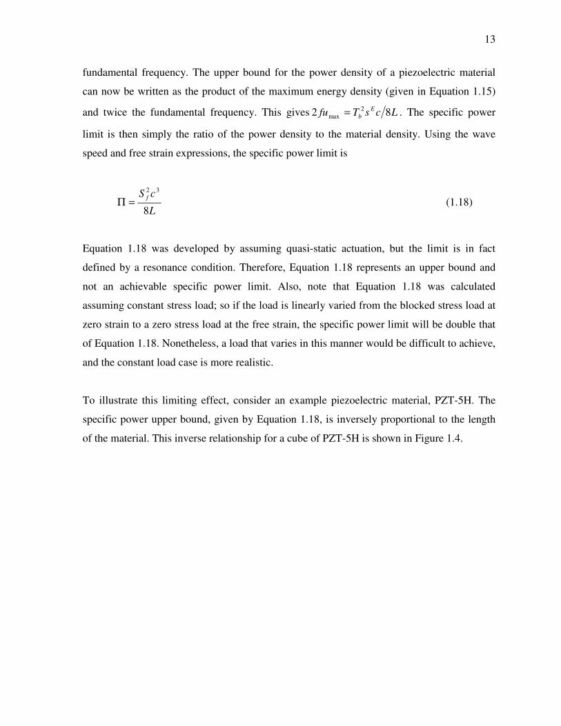
To illustrate this limiting effect, consider an example piezoelectric material, PZT-5H. The
specific power upper bound, given by Equation 1.18, is inversely proportional to the length
of the material. This inverse relationship for a cube of PZT-5H is shown in Figure 1.4.

14
Figure 1.4: Specific power versus its length for a piezoelectric element
Taking the length of the piezoelectric element as a measure of its size, the trend between
specific power and actuator size is an increase in specific power with decreasing actuator
size. The electromagnetic actuator has the opposite trend, and thus it appears that
piezoelectric actuators have potential for high specific power actuation on small size scales
where electromagnetic actuators perform poorly. Here lies the motivation for developing
piezoelectric actuators.
25.4 mm
1.0 mm
Theoretical estimation for a block of piezoelectric material
Electromagnetic actuators (100% duty cycle)

15
In addition to their specific power potential, piezoelectric actuators have other advantages
over conventional electromagnetic actuators. One chief advantage is that piezoelectric
materials do not fundamentally emit a magnetic field (although wires for powering the
piezoelectric material will emit a small magnetic field). This is important because large
magnetic fields that are inherent to electromagnetic actuators can interfere with sensitive
electronics in aircrafts. Another advantage is that piezoelectric materials can be designed to
accommodate high temperatures under which electromagnetic coils would fail (upwards of
200°C [3]). High temperature environments become a concern in many applications
including supersonic flight. Finally, piezoelectric actuator shapes are typically less
constraining than electromagnetic actuators, making them easier to fit into tight design
envelops.
1.2.3 Piezoelectric actuators
The projections in Figure 1.4 are far from what has been achieved in practice. This is because
the surrounding structure and coupling mechanism between a load and the piezoelectric
material has not been considered in the theoretical derivation of Equation 1.7. The
electromechanical response of piezoelectric materials is difficult to use directly in most
actuator applications; thus, the surrounding structure and coupling mechanism contribute
heavily to specific power performance degradation in most piezoelectric actuators. For
example, when a maximum electric field is applied to a soda can-sized block of piezoelectric
material, it can lift an entire car at a high rate (~0.5 m/s), but only the distance of the
thickness of a few human hairs (~100m).
This unique high force, high speed, and low displacement response of piezoelectric materials
is not directly conducive to most actuation applications. However, niche applications such as
active vibration control do exist wherein piezoelectric materials are directly coupled to
structures to effectively cancel or suppress their vibration. Another niche application is fuel
injector valves in engines. The short actuation stroke and high speed of piezoelectric
materials match well with the requirement of fuel injector valves and this application is
common in the automotive industry [4].

16
Instead of pursuing niche actuation applications, the work in this dissertation has addressed
the difficult problem of developing more general long-stroke piezoelectric actuators. To use
piezoelectric materials for long stroke actuation, either the material’s displacement must be
amplified or many actuation strokes of the material must be summed or accumulated over
time. For most applications, motion amplification alone will not result in adequate
displacement; and thus, a combination of motion accumulation and amplification is used. The
result is that, typically, a piezoelectric element is driven with a high frequency electric field
and its resulting repetitive field-induced strain is harnessed to drive a load. A simple
ratcheting mechanism shown below in a 1967 patent sketch by Breskend clearly illustrates
this basic motion accumulation principle [5, 6].
Figure 1.5: Breskend’s patent sketch of a motion-accumulating mechanism
The large discrete ratchet increments on the gear are unrealistic for the micrometer
displacements of a piezoelectric element; however, Figure 1.5 illustrates the basic principle
used by most high specific power piezoelectric actuators. While there are many types of
motion accumulation mechanisms, all of them work on a similar principle whereby
piezoelectric electric field-induced strain is accumulated to give a net continuous output
motion.
Piezoelectric element
Output rotation

17
The focus on developing motion accumulation mechanisms for high specific power
piezoelectric actuators is a recent pursuit. In fact, the primary efforts in this research area
began in the 1990’s when the Department of Advanced Research Projects Agency (DARPA)
funded its Compact Hybrid Actuator Program (CHAP). Improvements in high specific power
piezoelectric actuation resulted from the CHAP, yet progress is still needed to compete with
electromagnetic actuators. This dissertation presents a new actuator that overcomes many of
the limitations of these past designs and has the potential to improve upon the conventional
electromagnetic actuator’s specific power in the 1-100W power range.
1.3 Research approach and organization
The potential reward for developing a high specific power piezoelectric actuator is
significant, but it is a formidable challenge. In this research work, this challenge was
approached by studying past research literature and identifying the shortcomings and
potential of existing research work. Based on past research work, engineering intuition was
used to generate new ideas.
Because piezoelectric actuators are highly sensitive to factors such as backlash and friction
that are difficult to anticipate and theoretically model, theoretical evaluation at this stage of
the research would have been of limited use. Therefore, the process of developing the
actuator consisted of iterative experimental testing and modification. Once the actuator
design was established experimentally, improving it through experimentation would have
been a tedious process. In this case, the research effort shifted to modeling, simulation, and
design optimization.
This process of conceptual experimentation, modeling, and design optimization of the new
piezoelectric actuator is presented in the following dissertation. These pursuits are organized
into seven chapters, the first of which has already outlined the objectives and approach to the
research work. In Chapter 2, the origins of the piezoelectric effect are discussed. Particular
attention in this chapter is focused on developing the constitutive piezoelectric equations. In

18
this chapter, important properties of piezoelectric materials are also discussed in relation to
actuator applications.
Chapter 3 presents a survey of the most successful piezoelectric actuator designs. The
limitations of these past designs are discussed in an effort to define the direction and focus of
the new actuator development. Chapter 4 presents the new piezoelectric actuator concept and
the numerous prototypes that preceded it. Additionally, the merits, drawbacks, and potential
of the new actuator design are discussed in Chapter 4.
In Chapter 5, the application of this new actuator to a morphing aircraft structures application
sponsored by DARPA (Defense Advanced Research Projects Agency) and the Lockheed
Martin Corporation is discussed. In Chapter 6, a mathematical model of the actuator is
discussed in terms of a design optimization tool for improving the actuator. In chapter 6, the
performance potential of the new actuator design is also compared to electromagnetic
actuators. This dissertation concludes with Chapter 7, where the significance of the actuator
design and future work are described.
The body of work in this dissertation builds upon the culmination of 10 years of piezoelectric
actuator research work at The Pennsylvania State University in which the author has
participated for four years. The later two of these four years were spent developing the design
discussed in this dissertation.

Chapter 2
PIEZOELECTRIC THEORY
2.1 Origins of electric field-induced strain in ferroelectric materials
In piezoelectric actuator research, molecular-level crystalline structure interactions that
govern piezoelectric coupling are often overlooked for a material’s bulk electromechanical
coupling used to power piezoelectric actuators. Nevertheless, a rigorous understanding of
piezoelectric crystalline structure interactions provides valuable insight into aspects of
actuator design such as piezoelectric material selection and optimum driving conditions.
Therefore, this chapter discusses the molecular interactions that cause the piezoelectric
effect and the theory by which it can be described. In addition, various other topics
involving the practical use of piezoelectric materials in actuators are discussed. To introduce
these topics, this chapter begins with a brief historical overview of the piezoelectric effect’s
discovery and the ensuing material developments.
2.1.1 Historical overview of piezoelectricity
The piezoelectric effect was first discovered by the Curie brothers in 1880 [7]. Shortly
thereafter, Lord Kelvin described piezoelectric behavior using a rigorous thermodynamic
theory. A few years later, Woldenar Voigt built on Kelvin’s work by carrying out even more
detailed formulations, which are the basis for the development of the piezoelectric
constitutive equations in this chapter. At the time of Voigt’s work, there were only two
known piezoelectric crystals: Rochelle salt and potassium dihydrogen phosphate. These
crystals were impractical for most real-world applications due to their poor piezoelectric
properties—compared to the materials used today. During WWII, however, researchers in
Japan, England, Russia, and the United States independently discovered the high dielectric
constant of barium titanate. This spurred research interest in piezoelectric materials and
established an important connection between ferroelectricity and piezoelectricity that, in
turn, broadened the research field tremendously.

20
Shortly after the breakthrough of barium titanate, the focus in material development shifted
from single-crystal materials to polycrystalline or piezoceramic materials. Perhaps the most
important result of this shift in focus was the development of the strong and stable lead
zirconate titanate (PZT) piezoceramic. Since its discovery in 1952, PZT has been steadily
improved with various additives and it is currently the most prevalent piezoceramic. Its
discovery contributed heavily to the establishment of application-based piezoelectric
research, which is the focus of this dissertation.
The research focus on piezoceramic materials originated from the profound observation that
domain reorientations contributed heavily to the piezoelectric effect in polycrystalline
materials. For modern piezoelectric materials, these domain reorientations are equally as
important as the original piezoelectric phenomenon that the Curie brothers observed in
mono-domain salt crystals. However, in describing the origins of the piezoelectric effect and
its theoretical formulation, it is best to begin by considering mono-domain crystalline
structures. Following this discussion, domain reorientation in piezoceramic materials will be
addressed.
2.1.2 Crystal structure
By far the most studied piezoelectric mono-domain crystalline structure or single-crystal is
barium titnate (BaTiO3) [8]. Because BaTiO3 exhibits stable and linear electromechanical
coupling at room temperature and is readily grown in large single-crystals, it is repeatedly
referred to in the following discussion.
BaTiO3 has a perovskite crystalline structure consisting of eight barium atoms that form a
cube, six oxygen atoms located at the center of the cube’s faces, and one titanium atom at
the entire structure’s center.

21
Figure 2.1: Perovskite crystalline structure, a) unpolarized, and b) polarized,
Source: Waanders 1991
Each atom in the BaTiO3 is ionized and hence posses either a positive or negative electrical
charge. When an electric field is applied to the BaTiO3 structure, electrostatic forces cause
the anions to attract to the anode and the cations to attract to the cathode. This attraction
causes the atoms to shift slightly, giving rise to a net electrical polarity of the structure. In
such cases, each BaTiO3 cell is said to have an electric dipole. The formation of electric
dipoles, normally with the application of an electric field, is called electric polarization;
materials that can be polarized are said to be dielectric. Electric polarization of a material is
expressed qualitatively as the sum of the electric dipoles per unit volume (C/m^2).
In some cases, this ion shifting in the presence of an electric field causes not only
polarization, but also a geometric shape change of the crystals. If the geometric shape
change of the crystals occurs in an ordered manner, electromechanical coupling will result.
The specific relationship that governs the electromechanical coupling in dielectric materials
depends heavily on a material’s spontaneous polarization.
2.1.3 Spontaneous polarization
Spontaneous polarization is defined as a stable polarization of a crystal in the absence of an
external electric field. This occurs when the sum of electric dipole and elastic energies in a
crystalline structure results in a net energy minimum at a non-zero polarization. This is
a) b)

22
possible because the dipole energy is typically a quadratic function of the polarization, while
the elastic energy follows a fourth order relationship with polarization [9]. The combination
of these energies for BaTiO3 at room temperature and without an external electric field is
shown in Figure 2.2.
Figure 2.2: Energy functions in a dielectric material, Source: Uchino 1997
The shape of these energy functions (and in turn the spontaneous polarization) changes with
temperature. There is a critical point—known as the Curie temperature—that defines the
transition to a spontaneous polarization state from a state that was originally electrically
neutral. Above the Curie temperature, the crystal is electrically neutral and its
crystallographic phase is called paraelectric; below the Curie temperature, the crystal is
spontaneously polarized and this crystallographic phase is called ferroelectric. For BaTiO3,
the boundary between the ferroelectric and paraelectric phases is at 120ºC; therefore, it
occupies the ferroelectric phase when at room temperature. Materials with a ferroelectric
phase—and, more specifically, a spontaneous polarization that can be reversed with an
electric field—are referred to as ferroelectric materials.
2.1.4 Crystalline structures
In keeping with the fact that polarization results from a shifting of ions in the crystalline
structure, it follows that spontaneous polarization in the ferroelectric phase results in a stable
spontaneous shift or skew of the structure. Therefore, even in the absence of an electric
field, BaTiO3 will have a skewed structure while in the ferroelectric phase and a simple
cubic structure while in the paraelectric phase. Interestingly, the temperature not only

23
dictates the material’s phase, but it also influences the shape of the ferroelectric skewed
crystalline structure. In fact, depending on its temperature, BaTiO3 can occupy one of three
different spontaneously polarized skewed shapes. These shapes and their corresponding
temperature ranges for BaTiO3’s ferroelectric phase are shown in Figure 2.3.
Figure 2.3: Crystalline structures within the ferroelectric phase, Source: Ikeda 1996
Between BaTiO3’s 120ºC Curie temperature and 5ºC, it will have a tetragonal structure. In
the tetragonal structure, the O2- cations are shifted in a direction normal to one of the faces
of the cube, resulting in the elongation of the cubic cell along the direction of the shifted ion
(<001> or <010> or <100> or the other 3 equivalent inverses of these cubic directions).
Between 5ºC and -90ºC, BaTiO3’s structure is orthorhombic or monoclinic. Ions shifting in
this temperature range cause the diagonal on two opposing faces of the crystal to elongate
and the corresponding perpendicular diagonals to compress (<011> or other 11 equivalent
diagonal directions). Finally, below -90ºC, BaTiO3 has a rhombohedral structure. The
rhombohedral structure has an elongated diagonal that passes through the center of the
crystal (<111> or other 7 equivalent diagonal directions). Other perovskite ferroelectric
materials have similar structures to BaTiO3, but different transition temperatures and
degrees of spontaneous polarization [8].
Cubic

24
2.1.5 The piezoelectric effect
In the Section 2.2, the importance of the crystalline structure and spontaneous polarization
will be discussed in detail. At this point, however, this discussion of spontaneous
polarization leads to the distinction between the piezoelectric and electrostrictive effects.
The piezoelectric effect is strictly defined as linear coupling between an applied mechanical
stress and a resulting electric field. This specific electromechanical coupling only occurs
about a spontaneously polarized state; therefore, the piezoelectric effect is only observed in
the ferroelectric phase. In contrast, quadratic electromechanical coupling is observed
between an applied electric field and the resulting mechanical strain in the paraelectric
phase’s simple cubic structure. This is called the electrostrictive effect. Confusion often
surrounds the definition of the electrostrictive and piezoelectric terms because piezoelectric
materials can exhibit either a piezoelectric effect while in the ferroelectric phase, or an
electrostrictive effect while in the paraelectric phase.
In general, ferroelectric materials that have a Curie temperature below the ambient
temperature exhibit electrostriction, while materials with a Curie temperature above the
ambient temperature exhibit a piezoelectric effect. Both the piezoelectric and electrostrictive
effects are used in actuator and sensor applications. However, the linearity of the
piezoelectric effect makes it more attractive for most applications. Note that the temperature
dependence of the polarization and strain in the ferroelectric phase is called the pyroelectric
effect. The pyroelectric effect has been used in temperature sensors [10].
By these definitions, BaTiO3 is a ferroelectric material that can exhibit the piezoelectric,
electrostrictive, and pyroelectric effects. However, the electric dipoles in ferroelectric
materials do not always induce a mechanical strain, and hence, not all ferroelectric materials
are piezoelectric.

25
2.2 Phenomenology of piezoelectric materials
The discussion in this chapter has focused on the crystalline interactions that cause the
piezoelectric effect in certain single-crystal materials. This discussion has laid the
foundation for describing basic piezoelectric theory on which the development of
piezoelectric constitutive equations is based. In the following three sections, the
development of the piezoelectric constitutive equations is approached from a theoretical
thermodynamic perspective. Therefore the appropriate starting point is a mathematical
expansion of a ferroelectric material’s energy density associated with its dipole interactions
[9]. This energy expansion—called the “Landau free energy”—accounts for the unique
dielectric behavior of ferroelectric materials. Next, the net energy density of a piezoelectric
material will be considered by using the Gibbs free energy equation. In this case, the Landau
energy will be the dielectric energy component of the Gibbs free energy.
2.2.1 Landau theory
For simplicity, only the one-dimensional form of the dipole energy density expansion in the
absence of external stress will be used in this derivation. Considering this, the Landau free
energy expression is written as
...61
41
21
),( 642 +++= PPPTPF λβα (2.1)
The variable P is the polarization and , , and are temperature-dependent coefficients that
define the dipole interaction in a given ferroelectric material. In most dielectric materials,
only the first term is required to describe polarization. However, in ferroelectric materials,
two higher order terms are included to account for spontaneous polarization [9]. Note also
that the Landau energy is an even function. This is the case because a polarization reversal
will not change the dielectric energy density of the material.

26
For spontaneous polarization to exist, a polarization in the absence of an electric field must
result in a lower energy state than at zero polarization. Considering that determines the
curvature of the free Landau energy near zero polarization, this leads to the condition that
must be negative in the ferroelectric phase and positive in the paraelectric phase, passing
through zero at the so-called Curie-Weiss temperature, T0 (the relationship between the
Curie-Weiss temperature and the previously discussed Curie temperature will be developed
shortly). This temperature dependence of is explained physically by thermal expansion
and anharmonic lattice interactions (stiffness differences in opposing directions) in the
ferroelectric material. Therefore, the coefficient must be written as
C0
0 )(ε
θθα −= (2.2)
where C is a positive constant and 0 is the dielectric permittivity in a vacuum.
Aside from these initial observations and the definition of , further inspection of the free
Landau expression provides little insight into its description of the dielectric behavior of
ferroelectric materials. However, the usefulness of the Landau energy expression will
become clearer as expressions for various ferroelectric properties—such as electric field
spontaneous polarization, dielectric constant, and the critical paraelectric to ferroelectric
phase transition temperature—are derived.
The electric field can easily be found by taking the partial derivative of the Landau energy
with respect to polarization in dielectric materials. This definition gives:
53 PPPPF
E λβα ++=∂∂=
(2.3)
If no electric field applied to the material, the following expression must be satisfied.

27
0)( 42
0
0 =++−PP
Cλβ
εθθ
(2.4)
In the absence of an electric field, either the ferroelectric material will have zero polarization
in the paraelectric phase or it will have a spontaneous polarization in the ferroelectric phase.
Therefore, the spontaneous polarization must be given by
λεθθλββ
2/)(4 00
22 C
Ps
−−+−=
(2.5)
Most piezoelectric materials have a negative and a positive coefficient [9]. In this case,
the ferroelectric material is said to have a first-order transition between the ferroelectric and
paraelectric phases. Considering the first order transition and that the spontaneous
polarization must be a real number in the ferroelectric phase, the following condition must
be satisfied
0/)(4 002 =−− Cεθθλβ (2.6)
This in turn leads to
λεβθθ
40
2
01
C+= (2.7)
Equation 2.7 guarantees that the material will be in the paraelectric phase when the material
is above the 1 temperature. However, this condition only indicates the possible existence of
a spontaneous polarization and does not guarantee that it will be more stable then zero
polarization. To guarantee a spontaneous polarization, the Landau energy at the spontaneous
polarization must be less than or equal to zero [9]. Therefore, the more rigorous transition is
defined by setting the Landau energy to zero.

28
061
41
21 642
0
0 =++
−sss PPP
Cλβ
εθθ
(2.8)
Solving for the transition temperature in a similar manner as was previously done gives
λεβθθ
163 0
2
0
CC +=
(2.9)
Recall from Section 2.1.5 that this temperature—called the Curie temperature—defines the
transition between the paraelectric and ferroelectric phases. Notice that the Curie
temperature is slightly lower then 1θ , but greater than the Curie-Weiss temperature.
The described behavior of the temperature-dependent Landau energy is plotted in Figure
2.4.
Figure 2.4: Change in Landau energy with temperature, Uchino 1997
P
F

29
Notice that in Figure 2.4, the temperature 1θ indicates the point at which a local minimum or
a possible spontaneous polarization can exist, while the temperature C guarantees that the
minimum will be at a lower energy state then at zero polarization.
The dielectric permittivity of the material can also be derived from the Landau energy. The
permittivity in a dielectric material can be defined as the partial derivative of the electric
field with respect to the polarization, giving
42
0
531
PPDE λβα
εε++=
∂∂= (2.10)
In the paraelectric phase, the dielectric permittivity constant is generally taken about a zero
net polarization because the spontaneous polarization will be zero and electric field-induced
polarization will only contribute a small amount to the permittivity. Therefore, the
paraelectric permittivity can be given by
( )0θθε −= C (2.11)
(which is simply the Curie-Weiss law). From this, one can also infer that the coefficient is
in fact the impermittivity of the material.
The permittivity in the ferroelectric phase can be found in a similar way by setting the
polarization in Equation 2.10 equal to the spontaneous polarization from Equation 2.5. The
ferroelectric permittivity can then be given by
CC )(8
43
12
0 θθλβεε −+= (2.12)
The variation of the permittivity and spontaneous polarization with temperature are
graphically depicted in Figure 2.5.

30
Figure 2.5: Temperature dependence of spontaneous polarization and permittivity, Source: Uchino 1997
Although both the ferroelectric and paraelectric phases have been described in this section,
the piezoelectric effect occurs only in the ferroelectric phase. Therefore, it will be the sole
focus of the rest of this theoretical discussion. However, similar derivations for
electrostriction could be achieved by considering the paraelectric phase.
2.2.2 Gibbs energy and piezoelectric constitutive equations
The development of the constitutive equations for piezoelectric crystal will now be pursued
by considering the sum of the Landau free energy and energy contributions from electrical
displacements and stresses.
In the Landau derivations, the one-dimensional form of the energy expression was used
because in actuator applications the electric field is always applied in the polarization
direction. However, now that the elastic response of the material will be considered,
directions perpendicular to the electric field become important. In addition, with the
inclusion of the elastic response, a designation for the conditions that were used to define
constants such as the permittivity and compliance of a material becomes important. This

31
designation is typically made with the superscripts S, T, E, or D for constant strain, stress,
electric field, or polarization respectively.
The appropriate energy expression that includes electrical displacements and stress for a
piezoelectric material can be formulated using the Gibbs energy equation as
2
21
PTQTTsFG jjjiDij −−=
(2.13)
The first term in the Gibbs energy equation is, of course, the Landau dielectric energy
discussed in the previous section. The second term defines the elastic energy of the material,
where Dijs is the compliance matrix without polarization and jT is a stress vector. The last
term provides piezoelectric energy. For most piezoelectric materials, the piezoelectric
energy term is a quadratic function of the polarization and is also governed by a set of
piezoelectric constants Qj.
The two most basic constitutive equations that govern a piezoelectric material’s
electromechanical behavior can now be found by taking the partial derivative of the Gibbs
energy function with respect to the polarization and the stress vector which results in the
electric field and strain vector Si respectively. This gives:
PTQPPPPG
E jj253 −++=∂∂= λβα
(2.14)
2PQTsTG
S ijDij
ii +=
∂∂−=
(2.15)
Typically, these piezoelectric constitutive equations are written in terms of the dielectric
displacement D instead of the polarization. The relationship between the polarization and the
dielectric displacement is given by

32
PED += 0ε (2.16)
Since 0E is generally much smaller then the material polarization in this case, P and D are
used interchangeably [8].
Assuming that a small electric field is applied to the material in the ferroelectric phase, the
polarization of the material will be the sum of the polarization due to the electric field PE
and the inherent spontaneous polarization Ps. Using the interchangeability of the dielectric
displacement and polarization, the dielectric displacement is then given by
sE DDD += (2.17)
Substituting this dielectric displacement into Equation 2.14 and 2.15 gives
)(2)()()( 53sEjjsEsEsE DDTQDDDDDD
PG
E +−+++++=∂∂= λβα
(2.18)
2)( sEijDij
ii DDQTs
TG
S ++=∂∂−=
(2.19)
Relative to the spontaneous dielectric displacement Ds, the electric field-induced dielectric
displacement DE is usually assumed to be small. Considering this and Equation 2.4, the
constitutive equations can be linearized about a zero electric field to give
jsjE TDQDE 2−= α (2.20)
EsiSijDiji DDQDQTsS 22 ++= (2.21)

33
Recall that the coefficient is the temperature dependent dielectric impermeability of the
piezoelectric material and is written as Tε1 . The displacement due to the spontaneous
polarization, given by 2si DQ , is often omitted from the constitutive equations because it is
fixed with respect to the electric field. The coefficient si DQ2 dictates the piezoelectric
displacement coupling in the material and is usually written as Tjd ε , where jd are the
piezoelectric strain constants. Considering these modifications, the following constitutive
equations are obtained.
jTj
ET Td
DEεε
−= 1
(2.22)
ETj
jDiji D
dTsS
ε+=
(2.23)
Rearranging the Equations 2.22 and 2.23 and using the material compliance
relationship jiTij
Dij
Eij ddss
ε1+= , the a common form of the constitutive equations, are written
as
jjT
E TdED += ε (2.24)
EdTsS jjEiji += (2.25)
The piezoelectric strain constants are typically given in units of m/V, the compliance matrix
in m2/N, the permittivity in C/V-m, and the dielectric displacement in units of C/m2. As was
assumed during this derivation, Equations 2.24 and 2.25 are valid only for small electric
fields, displacements, and temperature variations. This means that if a piezoelectric
material’s temperature rises or if it experiences a large compressive load, the constitutive
equation’s coefficient will change.

34
2.2.3 Piezoelectric constitutive relations
At this point, it is appropriate to adopt a convention to denote the material’s axial directions
and polarization. This convention is shown in Figure 2.6.
Figure 2.6: Axis designation, Source: Waanders 1991
In this new convention, the polarization direction is always chosen to lie along the 3-axis.
The application of an electric field along the 3-direction can result in piezoelectric coupling
along any of the six directions shown in Figure 2.6. For a tetragonal structure, the crystal
will only deform along the three principle directions, whereas rhombohedral and
orthorhombic structures can also exhibit shear coupling. Such coupling is usually designated
with two subscript numbers [11]. For example, the d31 coupling coefficient relates an electric
field in the 3-direction to a strain in the 1-direction. By crystalline symmetry, the d31
coefficient will be the same as the d32 coefficient; therefore, only the d31 coefficient is
required to describe fully these two coupling directions. This idea is used though out the
following equations for both the elastic and permittivity constants. The full elastic,
piezoelectric, and dielectric coupling matrix can now be written as
=00000000
00000
333131
15
15
ddd
d
d
d ij (2.26)

35
=
E
E
E
EEE
EEE
EEE
Eij
s
s
s
sss
sss
sss
s
66
44
44
331313
131112
131211
000000000000000000000000
(2.27)
=T
T
T
Tij
33
11
11
000000
εε
εε (2.28)
These matrix constitutive equations are often furthered simplified to scalar equations to
represent the most commonly considered actuation scenarios such as the 31-mode and 33-
mode, which gives
3333333 EdTsS E += (2.29)
3333333 ETdD Tε+= (2.30)
and
3311111 EdTsS E += (2.31)
3331313 ETdD Tε+= (2.32)
In this form, these constitutive equations are now well-suited for modeling the behavior of
piezoelectric materials in most practical actuator applications.

36
2.2.4 Electromechanical coupling
The piezoelectric constitutive equations can be used to derive an important parameter called
the electromechanical coupling coefficient. The electromechanical coupling coefficient
reflects the effectiveness of a piezoelectric material at converting electrical energy into
mechanical strain energy and vice versa. The electromechanical coupling for a given loading
cycle is written as
energyinputenergyconverted
k =2 (2.33)
The electromechanical coupling coefficient can be derived in a number of different ways by
considering either electrical or mechanical loading and either electrical to mechanical or
mechanical to electrical energy conversion; however, each scenario leads to the same
coupling expressions. The most applicable approach for actuator applications is to use
electrical to mechanical energy conversion under a mechanical load. One such loading
cycle, shown in Figure 2.7, would involve the following sequence
(a) (b): Apply an electric field along the polarization direction and allow
the material to freely deform
(b) (c): Fix displacement of the material in coupling direction of choice
and remove the electric field
(c) (a): Remove the fixed displacement constraint and allow the material
to return to its initial state

37
Figure 2.7: Loading cycle for determine electromechanical coupling coefficient
This loading cycle will result in the following stress versus strain and electric displacement
versus electric field plots.
Figure 2.8: Mechanical and electrical loading curves
From point (a) to (b), the stress T0 remains at zero because the sample is unloaded.
Conversely, between points (b) and (c) the strain will be held fixed at some peak free strain
of S0. Under these conditions, the corresponding strain S0, stress T0, and electrical
displacement D0 can be computed from the constitutive equations. For the k33 coupling
coefficient, these constants are given as
0333
03 EdS = (2.34)
0333
03 ED Tε= (2.35)
EsEd
T33
03330
3 = (2.36)
(a) (b) (c)
(a)
(b)
(c)
E
D
D0
E0
(b) (c)
T
S
S0
T0 (a)

38
This loading cycle isolated the electrical input and mechanical output energy as is shown by
the shaded areas in the Figure 2.8 plots. These areas and their corresponding electrical and
strain energies are written as
2033
03
03 )(
21
21
EEDU Tinput ε== (2.37)
Eoutput sEd
STU33
203330
30
3 2)(
21 == (2.38)
The electromechanical coupling coefficient in the 33-mode can now be written as
ETinput
output
sd
U
Uk
3333
33233 ε
== (2.39)
Similarly, coupling coefficient in the 31-mode can be calculated as
ET sd
k1133
31231 ε
= (2.40)
An important distinction to draw is that electromechanical coupling is not the same as
electromechanical efficiency. This is because the dipoles in piezoelectric crystals behave
electrically similar to capacitive elements and therefore some of the electrical energy input
to the material for a given load cycle can be recovered.
2.3 Piezoceramics
For convenience and clarity, the Landau theory derivations in this chapter have focused on
piezoelectric single-crystals. However, in practical engineering applications, single-crystals
are rarely used because they are difficult (or, often, impossible at present) to manufacture

39
with desirable actuator properties. Instead of using single-crystals, most piezoelectric
actuators use piezoceramic materials that are conglomerate polycrystalline structures, made
from sintering single-crystals. These piezoceramic materials are relatively inexpensive and
are more durable than pure single-crystals. The following sections discuss the practical
concerns with manufacturing and using piezoceramics in actuators.
2.3.1 Piezoceramics versus single-crystals
Piezoceramic materials are fabricated by combining a fine powder of piezoelectric crystals
with water to form slurry. The slurry is poured into molds to form “green sheets.” The green
sheets are then pressed and fired at temperatures on an order of 1000ºC [9]. During this
firing process, regions or grains of single-crystals grow. The grain size is dictated by the
temperature and duration of the firing process. The material is then slowly cooled, thereby
allowing the spontaneous polarization to develop in the crystals. The spontaneous
polarization of the crystals cause them to align with one another in each grain. The regions
of grains that have similar crystal orientations are called domains. The domains also try to
align with one another and, in turn, take on a head-to-tail configuration according to Gauss’s
grain boundary theory. This causes some of the domains to have parallel alignment and
some to have perpendicular alignment to one another.
As would be expected, the polar direction of the domains is random after the initial
fabrication process. To reorient the domains to coincide with the geometry of the ceramic,
“polarization” of the sample is carried out. Piezoceramic polarization involves heating the
ceramic to just below its Curie temperature and applying a large electric field in the
direction of the desired polarization. The sample is then cooled while the electric field holds
the domains in position. In this process, not all of the domains become aligned with the
polarization direction and this misalignment in the crystalline structure creates an important
distinction between the piezoelectric behavior of piezoceramics and single-crystals.
In piezoceramics, the misaligned domains are not rigidly fixed in the crystalline structure,
but instead are to some extent free to reorient when loaded electrically or mechanically. The

40
domain reorientations cause large strains, which can enhance the material’s piezoelectric
response. This contribution to the net piezoelectric behavior is called the material’s extrinsic
response. Alternatively, the direct ion movement observed in single-crystals is called the
intrinsic response. All piezoceramics exhibit both intrinsic and extrinsic piezoelectric
behavior, while single-crystals only have an intrinsic response. This explains why some
piezoelectric ceramics have higher piezoelectric constants than their single-crystal counter
parts. The contributions of the extrinsic and intrinsic responses of piezoelectric materials is
dependent on the material type and crystalline structure. The degree of a piezoceramic’s
extrinsic response can affect the elastic and dielectric properties of a material. In general, an
increase in the extrinsic contribution to the material response will result in a decrease in
material stiffness and an increase in its permittivity.
Note that if a large electric field is applied in the opposite direction to the poling direction,
the domains will rotate 180º. The electric field required to cause a complete 180º domain
reorientation is called the coercive field.
2.3.2 Dopants
The contribution of extrinsic domain reorientations to the net piezoelectric response can be
controlled to some degree by adding dopants to the ceramic. Dopants induce vacancies in
the grain walls of piezoceramics, which in turn create auxiliary dipoles in the ceramic.
Depending on how large the dipole charges are, they can act to stabilize or destabilize the
domain walls. Stable domain walls limit domain reorientations, while less stable domain
walls promote domain reorientation, and hence, increase the extrinsic response of the
piezoceramic. Dopants that destabilize the domain walls are called donor additives; dopants
that stabilize the domain walls are called acceptor additives. Stabilizing the domain walls
with acceptor dopants is referred to as the domain pinning; destabilizing with donor dopants
is called depinning. Piezoceramics with stable domain walls and a small extrinsic response
are referred to as “hard” materials, while materials with a large extrinsic response are “soft”
piezoceramics. Hard piezoceramics tend to have lower piezoelectric constants and lower
hysteresis while soft materials have higher piezoelectric constants and higher hysteresis.

41
Therefore, a piezoceramic can be tailored to give a desired response by doping it with
different type of additives.
2.3.3 Hysteresis
Domain reorientations introduce hysteresis into the piezoelectric behavior of piezoceramics.
This is because after an electric field is applied to a piezoceramic, some of the domains that
reorient with the field do not return to their original misaligned state. The hysteresis for soft
piezoceramic is shown in the Figure 2.9 strain versus voltage plot.
Figure 2.9: Hysteresis in piezoelectric effect, Source: Pickelmann 2001
Hysteresis in piezoceramics can cause significant positioning and self-heating problems for
actuator applications [12]. The heat energy generated in the material due to the domain
reorientations is typically characterized by the loss factorδ . The tangent of the loss factor is
may be defined as the ratio of the energy that is lost as heat energy to the input electrical
energy, which is given as
energyinputenergyheat=δtan (2.41)
For high frequency and high duty cycle applications, low loss factor materials and managing
the temperature of the ceramic by designing for adequate heat transfer are critical to prevent
Voltage
Strain

42
overheating and damage to the ceramic. Higher loss factor materials are generally used for
applications where a high piezoelectric constant is important and the driving frequency or
duty cycle is low enough to prevent over heating.
2.3.4 Effect of compressive stress
Interestingly, the extrinsic response (and, in turn, the hysteresis behavior) of a material can
be altered to some degree by adding a bias stress to the piezoceramic. Consider applying a
compressive stress along the polarization direction: The compressive stress will cause some
of the originally aligned domains to become misaligned, which effectively increases the
extrinsic response of the ceramic. Such a compressive stress will also slightly lower the
stiffness of the material. In practice, bias stress is typically applied to piezoceramics to
protect them from encountering tensile stress. However, care should be taken when applying
bias stress to a ceramic because large stresses will cause irreversible misalignment of the
domains, resulting in depolarization.
2.3.5 PZT
The most common piezoceramic material, PZT (Pb(ZrTiO3)), is a ceramic blend of the
PbTiO3 and PbZrO3 crystals. Different ratios of each component and different dopants give
quite different material properties. Most PZT ceramics have excellent piezoelectric
properties, are durable, and are relatively inexpensive to manufacture.
Despite hysteresis and nonlinearity inherent to the extrinsic piezoelectric effect, for low
electric fields, PZT exhibits a similar piezoelectric coupling to that of mono-domain
piezoelectric material, and therefore, the same constitutive equations derived in Section
2.2.3 are typically used to define its response. Coefficients in the piezoelectric constitutive
equations for a few of the example piezoceramic materials are shown in Table 2.1.

43
Table 2.1: Material properties of PZT, Source: Sinoceramics Inc.
Material types PZT-4 PZT-8 PZT-5A PZT-5H
Properties very hard hard soft very soft
k33 0.68 0.68 0.71 0.76 Coupling Coefficients
k31 0.33 0.34 0.34 0.4
d33 310 280 450 630 Piezoelectric Constants
(x10-12 m/V) d31 -125 -105 -170 -275
Dielectric constants 33T/0 1150 1000 1800 3300
Dissipation factor (%) Tan 0.4 0.2 1.6 1.3
s11E 12.7 11.6 13.5 16.9 Elastic constants
(x10-12 m2/N) s33E 15.2 14.1 20 19.6
Poison's ratio E 0.33 0.33 0.35 0.34
Curie temperature (oC) Tc 308 320 310 250
Density (kg/m3) 7700 7700 7600 7700
In Table 2.1, the material PZT-8 is very hard and thus has a relatively low piezoelectric
constant and low loss factor, while PZT-5H is very soft and has a high piezoelectric constant
and high loss factor. Note that because the dielectric and elastic constants are also are
affected by the material hardness, the coupling coefficients are nearly the same regardless of
the material type.
2.4 Piezoceramic actuators
Prior to this section, piezoelectric theory was presented in a general manner, without specific
regard to actuator applications. In this section, the focus shifts to the implementation of
piezoceramics as practical actuators. For example, instead of focusing on the strain, stress,
and electric field, of piezoceramic, the extensive properties of a block of ceramic such as
displacement, force, and voltage is addressed.

44
2.4.1 Characterizing a piezoelectric material’s actuation capability
In this accord, it is appropriate to begin by considering the sample block of piezoceramic
shown in Figure 2.10.
Figure 2.10: Piezoceramic block
Assume the actuation direction to be coincident with the electric field and polarization
directions (33-mode). The rectangular block’s height, length, and width are given by h, l,
and w, respectively.
If a positive voltage is applied across the electrodes, the block will elongate along the 3-
direction and contract in the 1,2-directions. Note the block may also exhibit shear coupling
if it has a rhombohedral or orthorhombic structure. The elongation and contraction of the
block can be calculated using the constitutive equations and the definitions of stress, strain,
and electric field. The maximum elongation in the 3-direction, in the absence of an external
load, for a given voltage U is called the “free displacement” and is given by
UdhEdhTShf 3333333 )0( ====∆=δ (2.42)
Likewise, if the displacement is constrained while a voltage is applied to the block, a value
for the maximum force that the piezoelectric block can produce is determined. This value is
called the “blocking force” and is given by
Poling axis
3
2
1
h
w l
h
U

45
UhsAd
swlEd
wlSTF EEb33
33
33
33333 )0( ==== (2.43)
where the cross-section of the ceramic is generalized as area A instead of the product of the
width and length. Similar relations can be found in the two other orthogonal contraction
directions. However, this discussion focuses only on the 33-mode actuation for simplicity.
Recall from the constitutive equation derivation that the piezoceramic behaves nearly as a
linear-elastic material. Therefore, the stiffness of the piezoceramic block, KE is simply the
ratio of the blocking force to the free displacement, which gives
hsAF
K Ef
bE
33
==δ
(2.44)
A similar set of blocking force, free displacement, and stiffness expressions could be found
for d31 coupling.
Assuming that the piezoceramic behaves as a linear elastic material, the block’s one-
directional behavior can be represented as a spring of stiffness KE. This is shown in Figure
11.
Figure 2.11: Equivalent spring model
KE
f
Fb

46
If a voltage is applied to the block in the absence of an external load, the equivalent spring
model will extend according to the simple stiffness relationship
Eb
f KF=δ (2.45)
When a load L is applied to the block, the spring will no longer extend to the free
displacement, but will instead move a smaller distance given by
Eb
L KLF −=δ (2.46)
Notice that the free displacement and blocking force are proportional to the voltage, while
the stiffness is independent of the applied voltage. This simple spring behavior is commonly
illustrated with the force versus displacement plot, given in Figure 2.12.
Figure 2.12: Force displacement characterization of a piezoceramic
KE
Increasing voltage
Force (F)
Fb
f
Displacement ()
L
L

47
The line connecting the free displacement and the blocking force for a given external load
and applied voltage represents the maximum displacement that the spring will extend. An
increase in the voltage will shift the line in Figure 2.12 without changing its slope.
2.4.2 Multilayer devices
With this spring model in mind, a practical actuator example application can now be
described. Consider using a piezoelectric element to open a fuel injector valve in an internal
combustion engine. The free displacement necessary to open the valve is on an order of 15
µm. Now consider achieving this free displacement with the 33-mode (coincident
polarization, applied electric field, and actuation direction) of a piezoceramic block. If a
maximum electric field of 1000 V/mm is applied to the block, the block minimum height
can be calculated to be 23.8 mm for PZT-5H. To generate the 1000 V/mm electric field, a
large 23.8 kV would be required. Clearly, it would be difficult to design the power
electronics to switch such voltages dynamically. In addition, preventing shorting of 23.8 kV
to other components would be a concern.
2.4.2.1 Piezoelectric stack actuation
A good method of decreasing the driving voltage while maintaining a large electric field is
to alternately stack layers of piezoceramic and electrode. Under this circumstance, the
piezoelectric actuator would have a high charge density and manageable driving voltage.
These multilayer devices are called piezoelectric “stacks.”
Piezoelectric stacks are manufactured using two different methods. The first method consists
of interlaying electrodes between green sheets before firing the ceramic to produce co-fired
stacks. The second method involves laying electrodes on already-fired piezoceramic layers
and then bonding the layers together. Thicker ceramic layers are used in the bonded stacks
due to the intensive fabrication process. Bonded stacks have slightly higher piezoelectric
coupling properties because of the lower number of layers and the lower percentage of
electrode material; however, this is at the expense of the level of driving voltages [3]. Co-

48
fired stacks are fabricated in an automated process and typically are lower in cost than the
bonded stacks but are difficult to manufacture in heights greater then 2 inches. Regardless of
the fabrication process, stacks can be manufactured in many different shapes including
tubes, cylinders, and rectangular blocks. Two example piezoelectric stacks are shown in
Figure 2.13.
Figure 2.13: a) Example co-fired stack, b) bonded stack
The electrode layers are critical components in stack actuators because they conduct
electricity well and handling repetitive strain cycling (recall that piezoceramic layers
contract in the 1-direction). There are several different materials that can be used for the
electrodes but the most common is silver-palladium. Palladium is expensive and it often is a
driving cost in manufacturing stacks.
Electrodes have a finite thickness and elasticity that is important to account for in the
characterizing stack actuator’s piezoelectric response. When the stack does not have an
external load, the stack displacement will be unaffected by the electrode stiffness. However,
the series electrode stiffness will degrade the blocking force of the stack actuator. Assuming
the electrode stiffness behaves in a linear-elastic manner, the net stiffness of the actuator
decreases as shown in Figure 2.14.
a) b)

49
Figure 2.14: Effect of including electrode stiffness in spring model
A new equivalent stack spring model can be generated by letting the height (h) be the
product of the piezoceramic layer thickness (tp) and the number of layers (n) and by
modifying the blocking force to account for the stiffness of the electrodes. The new blocking
force can be computed by first letting the 1 be the total displacement of the electrodes under
a the new blocking force and letting 2 be the displacement of the ceramic layers with a
blocking force. This gives the following two equations.
21ˆ δδ E
eb KKF == (2.47)
+=+=
e
E
f KK
1221 δδδδ (2.48)
where Ke is the net stiffness of the electrode layers. Solving for 2 in Equation 2.48 and
substituting it back into Equation 2.47 gives a new blocked force of
Force (F)
Fb
f
bF
KE
Ke
Displacement ()
Fb
Piezoceramic
layers
Electrode
layers

50
( ) fe
E
E
b KKK
F δ+
=1
ˆ (2.49)
The stiffness of the electrode layers is simply given by
eee snt
AK = (2.50)
and the new free displacement equation is given by
Undf 33=δ (2.51)
which leads to a blocked force of
( )UtststsAd
Fp
Eeep
Eb3333
33
1ˆ
+= (2.52)
Clearly, it is best to have the least number and thinnest layers possible. Typically, electrode
layers are very thin and can be neglected in this model, but in co-fired stacks, the high
number of layers can result in important electrode stiffness.
2.4.2.2 Stack pre-compression
The electrode layers in stacks tend to make stacks fragile under flexural and tensile loads,
and thus, are used only in uni-axial compressive loaded configurations. To protect stacks
from encountering tensile or bending loads in real actuator applications, biasing compressive
loads are often applied to stacks. Such bias loading can be applied in any number of
different ways with devices such as a pneumatic or hydraulic cylinder, large weight, or
spring. However, bias loading is most conveniently applied with a parallel spring stiffness.
The parallel spring is usually integrated in a housing that surrounds the stack. However, a

51
unique way to apply the bias compression is to use a flexure assembly that serves a duel
purpose as a motion amplifier. Examples of pre-compression assemblies are shown below in
Figure 2.15.
Figure 2.15: a) Amplified bias compression assembly, b) in-line bias compression
The effect of the bias compression stiffness can be described using a similar method as was
used for considering the electrode stiffness. Here, instead of degrading the blocking force,
the preload stiffness will reduce the free displacement. Again, the graphical presentation of
the spring model shown in Figure 2.16 is useful for this discussion.
a) b)

52
Figure 2.16: Effect of including bias compression to stack spring model
The spring stiffness of the pre-compression is bK . The new stiffness of the entire stack
actuator is just the sum of the pre-compression and the stack stiffness from Equation ss
giving a composite stiffness of
( ) ( )pE
eepEb
eE
E
bE
tstsntsA
KKK
KKK
3333 11ˆ
++=
++= (2.53)
The degraded free displacement fδ , is the ratio of the stack blocking force to the new
composite stiffness giving
( )( ) U
nAtststsK
tstsd
K
F
pE
eepE
b
pE
ee
Eb
f 11
1ˆˆ
ˆ3333
3333
+++
==δ (2.54)
Notice that it is best to have a low bias compression stiffness to achieve the greatest free
displacement. In addition, notice that to achieve a high bias compression, while minimizing
Force (F)
Fb
f Displacement ()
bF
fδ
EK
KE
Ke
Kb

53
its affect on limiting the free displacement, a low stiffness and long displacement bias
compression spring is best. In such, the bias compression spring is attempting to replicate
the behavior of an optimum constant force compressive load.
Note that adding a compressive load to piezoceramic generally increases its piezoelectric
constants because the domains are forced into a less oriented state, and thus the net effect of
a bias spring depends on the piezoceramic material properties, the initial bias compression,
and the stiffness bias spring [10].
2.4.2.3 Dynamic operation
At low drive levels, up to 1010 cycles are achievable with the current state of the art
piezoelectric stacks [3]. This equates to 28,000 hrs of operation at 100 Hz. The lifetime limit
is typically associated with local stress concentrations (due to factors such as the termination
of electrode layers in co-fired stacks) in the piezoceramic that lead to cracking and
eventually insulation break down or rupturing of the electrodes [13].
Another consideration in the dynamic operation of stacks is resonance. In particular, damage
can occur from tensile loading of the ceramic during resonant vibration, regardless of the
bias compression applied to a piezoelectric stack. This is because amplification factors on
upwards of 10 can be observed at frequencies near the first natural mode. Such motion
amplification would cause the stack layers to undergo tensile loading and possibly
delaminate. Therefore, it is important to avoid the resonance modes of a stack.
The first longitudinal mode of the stack and bias compression assembly should be
considered for determining an upper bound for the driving frequency. This is usually the
case because the mass associated with the bias compression housing generally causes the
first natural mode of the combined stack and bias spring to be at a lower frequency than that
of the ceramic material alone. In addition, because the height dimension of stacks are
typically greater than their width or length dimensions, the 33-mode is usually of concern
rather than the 31-mode.
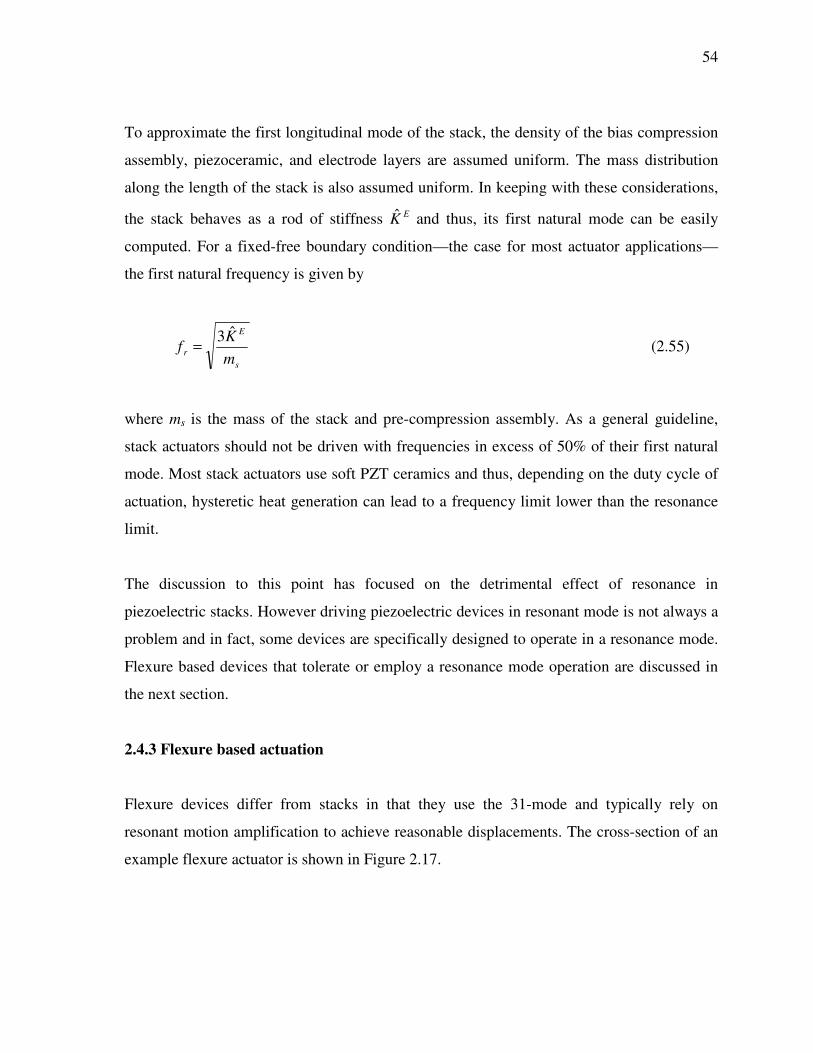
54
To approximate the first longitudinal mode of the stack, the density of the bias compression
assembly, piezoceramic, and electrode layers are assumed uniform. The mass distribution
along the length of the stack is also assumed uniform. In keeping with these considerations,
the stack behaves as a rod of stiffness EK and thus, its first natural mode can be easily
computed. For a fixed-free boundary condition—the case for most actuator applications—
the first natural frequency is given by
s
E
r mK
fˆ3= (2.55)
where ms is the mass of the stack and pre-compression assembly. As a general guideline,
stack actuators should not be driven with frequencies in excess of 50% of their first natural
mode. Most stack actuators use soft PZT ceramics and thus, depending on the duty cycle of
actuation, hysteretic heat generation can lead to a frequency limit lower than the resonance
limit.
The discussion to this point has focused on the detrimental effect of resonance in
piezoelectric stacks. However driving piezoelectric devices in resonant mode is not always a
problem and in fact, some devices are specifically designed to operate in a resonance mode.
Flexure based devices that tolerate or employ a resonance mode operation are discussed in
the next section.
2.4.3 Flexure based actuation
Flexure devices differ from stacks in that they use the 31-mode and typically rely on
resonant motion amplification to achieve reasonable displacements. The cross-section of an
example flexure actuator is shown in Figure 2.17.
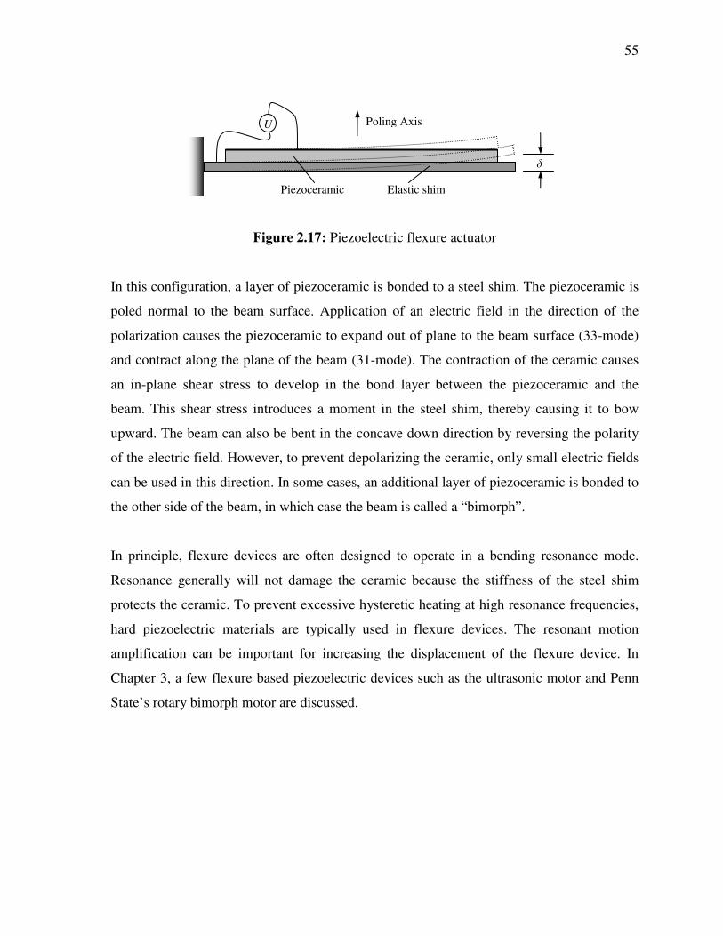
55
Figure 2.17: Piezoelectric flexure actuator
In this configuration, a layer of piezoceramic is bonded to a steel shim. The piezoceramic is
poled normal to the beam surface. Application of an electric field in the direction of the
polarization causes the piezoceramic to expand out of plane to the beam surface (33-mode)
and contract along the plane of the beam (31-mode). The contraction of the ceramic causes
an in-plane shear stress to develop in the bond layer between the piezoceramic and the
beam. This shear stress introduces a moment in the steel shim, thereby causing it to bow
upward. The beam can also be bent in the concave down direction by reversing the polarity
of the electric field. However, to prevent depolarizing the ceramic, only small electric fields
can be used in this direction. In some cases, an additional layer of piezoceramic is bonded to
the other side of the beam, in which case the beam is called a “bimorph”.
In principle, flexure devices are often designed to operate in a bending resonance mode.
Resonance generally will not damage the ceramic because the stiffness of the steel shim
protects the ceramic. To prevent excessive hysteretic heating at high resonance frequencies,
hard piezoelectric materials are typically used in flexure devices. The resonant motion
amplification can be important for increasing the displacement of the flexure device. In
Chapter 3, a few flexure based piezoelectric devices such as the ultrasonic motor and Penn
State’s rotary bimorph motor are discussed.
U Poling Axis
Elastic shim Piezoceramic

Chapter 3
SURVEY OF PIEZOELECTRIC ACTUATORS AND MOTORS
This chapter discusses techniques for harnessing the unique electric field-induced response
of piezoelectric materials to produce large stroke, rotational or linear actuation. Means for
accomplishing this were briefly discussed in Chapter 1 wherein the “motion rectification”
concept was introduced. Because developing a new improved motion rectification
mechanism is the primary topic of this dissertation, this chapter provides a thorough survey
of past piezoelectric actuator and motor motion rectification designs. The drawbacks and
desirable characteristics of these designs are outlined to help justify the direction of the
research pursuits in this dissertation. Additionally, historical milestones in the development
of piezoelectric actuators and motors are discussed to recognize important researchers who
have contributed to this field.
3.1 Types of piezoelectric actuators and motors
There are hundreds of long stroke piezoelectric actuator and motor designs and, to provide a
concise overview of them, it is useful to classify them according to their basic operation
principles. Borrowing from Hagood, the classification in Figure 3.1 of piezoelectric
actuators and motors is adopted for the following discussion [14].

57
Figure 3.1: Types of piezoelectric actuators and motors
Hagood broadly categorized piezoelectric motors and actuators as either quasi-static or
ultrasonic devices. Quasi-static devices are further classified as active clamping inchworms,
passive clamping ratchet-type devices, or piezoelectric pumps. Ultrasonic devices are
similarly subdivided into the standing wave and traveling wave device categories.
Both quasi-static and ultrasonic devices operate by driving piezoelectric elements with a
high frequency periodic electric field and harnessing or rectifying their resulting periodic
field-induced strain to drive continuously a mechanical load. However, differences between
ultrasonic and quasi-static devices lie in the way the rectification is accomplished.
In general, quasi-static rectification is achieved by repetitively accumulating a unidirectional
portion of the driving element’s periodic mechanical output. This is generally accomplished
by alternating the output load path from a piezoelectric element while it is driving and to
ground while it is relaxing. By doing so, the load is repetitively stepped forward in
correspondence with the periodic excitation of the piezoelectric driving element. Quasi-
static actuators are generally driven at frequencies below their fundamental natural
frequency. In this low frequency range of 100-1000 Hz, soft high strain piezoceramics are
used to maximize the material’s quasi-static power output.
Piezoelectric actuators/motors
Standing wave
Traveling wave
Ultrasonic
Hydraulic pumps
Quasi-static
Ratchet-type (Passive clamps)
Inchworm-type (Active clamps)

58
On the other hand, ultrasonic devices use piezoelectric elements to excite a stator in a
resonant mode such that a structural traveling or standing wave develops in the stator. The
stator’s periodic wave motion is in turn rectified by configuring it to come into frictional
contact with a rotor. The stator is typically designed so that its resonant driving mode is in
the 10-100 kHz frequency range. At these high frequencies, low loss or hard piezoelectric
materials are used.
3.2 Ultrasonic motors
There are many different ultrasonic actuator and motor designs, but they can generally be
described as either standing wave or traveling wave devices. The primary difference
between these two types of ultrasonic devices lies in their stator designs.
3.2.1 Standing wave motors
The first standing wave ultrasonic motors, and for that matter one of the first piezoelectric
motors, was conceptualized in 1948 by Williams [15]. His design had a rectangular tube
shaped stator with piezoelectric elements bonded to its sides. The piezoelectric elements
bend the tube stator such that a standing wave wobble motion develops in the rotor. The
wobble motion of the stator comes into frictional contact a rotor shaft, located inside the
tube, thereby driving it in a rotational fashion. William’s patent sketches are shown in
Figure 3.2.

59
Figure 3.2: Standing wave wobble motor, Source: Williams 1948
William’s wobble motor concept did not receive attention until the 1990’s when Uchino at
Penn State University implemented the design on a miniature size scale (~2 mm stator
diameter). Uchino’s miniature motor and its corresponding performance plot are shown in
Figure 3.3.
Figure 3.3: a) Uchino’s miniature piezoelectric motor and b) performance, Source: Uchino 1990
a) b)

60
Uchino’s motor produced a 1.8 N-mm stall torque, a 14.3 RPS free speed, and a 60 mW
maximum power output [16]. The peak power output corresponds to a large 150 W/kg
specific power. This is the highest reported specific power of any piezoelectric motor or
actuator. However, the small size of Uchino’s motor has limited its application to a few
specialized medical devices. As MEMS technology improves, Uchino’s motor could
become more important in the coming years.
3.2.2 Traveling wave motors
The second class of ultrasonic motors discussed here is traveling wave or propagating wave
motors. Traveling wave motors use piezoelectric elements bonded to a disc shaped stator to
excite a resonant mechanical wave, which propagates through the stator. As the traveling
wave propagates, a point on the stator’s surface follows a closed elliptical path. The peaks of
the stator waves come into frictional contact with the rotor, thereby driving the rotor in the
opposite direction to the propagating wave. The operating principle of the traveling wave
ultrasonic motor is illustrated in Figure 3.4.
Figure 3.4: Schematic of traveling wave motor
The most notable features of the traveling wave concept is that it exhibits a static self-
locking condition, can output high torque at low speeds, and can be manufactured in a
variety of different configurations, including a unique ring shape. Development of the most

61
common ring-shaped traveling wave ultrasonic motor is often credited to Sashida [17].
However, many researchers published ultrasonic motor designs in the late 1980’s.
The traveling wave motor has been successfully used in numerous applications, the best
known of which is Nikon auto focus camera lens. In addition, ultrasonic motors—
manufactured by Shinsei Corporation—were used as key actuation components in Northrop
Grumman’s DARPA Smart Wing program [18]. The Shinsei Corporation is currently
commercially selling ultrasonic motors at cost of about $600 (net cost for motor and power
supply). An exposed section of the Shinsei ultrasonic motor is shown in Figure 3.5.
Figure 3.5: Shinsei traveling wave motor, Source: Shinsei Inc. 2004
The Shinsei motor produces a 5 W peak power at a 0.5 N-m rated load. This peak power
corresponds to a specific power of 19.2 W/kg (not including power electronics). The speed
versus torque plot for this motor is shown in Figure 3.6.

62
Figure 3.6: Shinsei motor speed versus torque performance, Source: Shinsei Inc. 2004
In Figure 3.6, notice that there are “normal” and “short term” operation regions. In the
normal or low load operation region, the motor can operate for relatively long time periods.
However, in the short term operation region, slipping between the stator and rotor causes
wear. Wear of the stator and rotor reduces torque output and in turn its life. To improve
motor life, special wear resistant materials are used for the stator and rotor contact surfaces.
In spite of this, the Sensei motor’s life is rated at 1,000 hrs at the 0.5 kgf-cm (4.9 N-m) load.
A similar short life is observed for all ultrasonic motors that are based on the friction driving
mechanism. Considering that conventional electromagnetic motors can operate for upwards
of 20,000 hrs, the short life of ultrasonic motors is a significant drawback that limits them to
applications wherein the required duty cycle is low or a motor’s short life is acceptable. This
is an important limitation of ultrasonic devices that makes quasi-static devices more
attractive for some applications. This drawback is also the reason that the work in this
dissertation has focused on quasi-static actuator development.

63
3.3 Quasi-static actuators and motors
In Section 3.2, long stroke piezoelectric actuation was discussed in terms of harnessing high
frequency (10-100 kHz) piezoelectric mechanical output using friction based motion
rectification techniques. This section discusses a different strategy for rectifying, wherein
periodic piezoelectric mechanical output is quasi-statically rectified using accumulator
mechanisms. Of the three quasi-static type accumulation mechanisms (inchworm, ratchet,
pump), the most straightforward to describe, and hence what this section begins with, is the
inchworm.
3.3.1 Inchworm actuators
Inchworm actuators are named after the inchworm organism that moves using alternating
extension of its body and intermittent clamping of its feet. Inchworm actuators work on a
similar principle, wherein actuation of a piezoelectric element is analogous to the extension
of the worm’s body and the active clamps are analogous to the worm’s feet. Active clamps
typically use piezoelectric elements to actively apply a clamping force.
The sequential actuation of the piezoelectric driving element and active clamps necessary to
produce long stroke actuation is shown in Figure 3.7.

64
Figure 3.7: Inchworm actuator stepping sequence
Periodic repetition of the sequence, leads to a stepping motion and on average continuous
long stroke actuation. This is illustrated in Figure 3.8, wherein an example time history of a
piezoelectric driving element and its accumulated output is shown.
Figure 3.8: Example time history showing the mechanical motion output from an inchworm actuator
Direction reversal is accomplished by changing the phase between the active clamps and
driving element.
Piezoelectric driving element
Clamp
Load
Clamp
Unloaded output displacement
Time
Periodic electric field applied to piezoelectric driving element
Piezoelectric element driving Piezoelectric element recoiling

65
Locher was the first to document an inchworm-type actuator in his 1967 patent [19]. Ten
years later Burleigh Instruments successfully commercialized Locher’s actuator design and
trademarked the name InchwormTM. The Burleigh inchworm was designed for precision
positioning applications and their latest actuator achieves an impressive 0.1 nm positioning
resolution. A picture and patent sketch of the Burleigh inchworm is shown in Figure 3.9.
Figure 3.9: Burleigh’s latest inchworm, Source: Burleigh Inc.
Burleigh’s state-of-the-art inchworm actuator produces a 110 N blocked force and a 1.7 W
power, which corresponds to a 19 W/kg specific power. This actuator’s performance is
shown in the Figure 3.10 by the EM2-HRM-inchworm curve.
Active clamps
Driving element

66
Figure 3.10: The Burleigh inchworm’s power versus speed performance, Source: Burleigh Inc.
The primary limiting factor for the performance of inchworms is the force that can be
delivered from the piezoelectric driving element to the output load. Force delivered to the
load is determined by the clamp holding force, which in turn dependents on the force
exerted on the clamp’s contact surfaces and the surface’s friction characteristics.
In recent years, considerable design effort has been devoted to improving active clamps [20,
21]. One of the more successful clamp concepts was proposed in a 1990 patented by Murata.
Murata’s concept used ridges on the clamp’s contact surfaces to increase their effective
coefficient of friction [22]. Later UCLA researchers implemented this concept using micro
ridges etched onto the clamp’s surfaces [23]. The Murata and UCLA inchworm concepts are
shown in Figure 3.11.
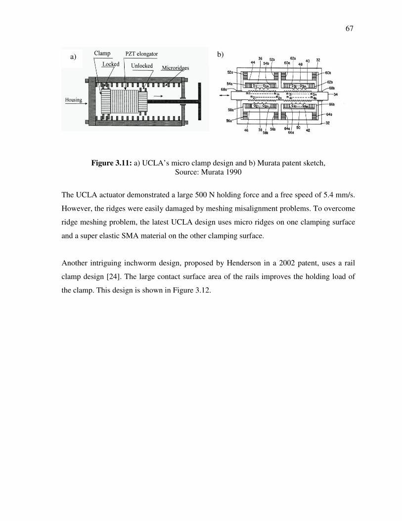
67
Figure 3.11: a) UCLA’s micro clamp design and b) Murata patent sketch, Source: Murata 1990
The UCLA actuator demonstrated a large 500 N holding force and a free speed of 5.4 mm/s.
However, the ridges were easily damaged by meshing misalignment problems. To overcome
ridge meshing problem, the latest UCLA design uses micro ridges on one clamping surface
and a super elastic SMA material on the other clamping surface.
Another intriguing inchworm design, proposed by Henderson in a 2002 patent, uses a rail
clamp design [24]. The large contact surface area of the rails improves the holding load of
the clamp. This design is shown in Figure 3.12.
a) b)

68
Figure 3.12: Henderson’s rail clamp design, Source: Henderson 2002
Other highly refined inchworm designs include the H3DB inchworm developed at the
Center for Acoustics and Vibration [25, 26]. The unique feature of the H3DB is flexure
hinge joints that stiffen the clamping mechanisms [11]. The H3DB, shown in Figure 3.13,
produced a blocked force of 140 N and a free speed of 1 mm/s.

69
Figure 3.13: H3DB inchworm actuator
In the described inchworm actuators, power electronics for the active clamps are required in
addition to that for the piezoelectric driving element. Because piezoelectric active clamp
elements typically have similar power requirements as the driving element, the power
electronics for inchworms are typically large (3 times that of other piezoelectric devices
such as ratchet-type motors). In addition, the power consumed in operating the clamps
reduces inchworm’s electro-mechanical actuation efficiency.
To aid in managing the power electronics issue, researchers have proposed using a
combination of magnetostrictive (introduced in Section 1.2.1) and piezoelectric clamping
elements [27, 28]. The inductive dynamics of the coils for magnetostrictive elements and the
capacitance of piezoelectric elements can be couple in a single resonant circuit to simplify
the power electronics.
Active clamps Driving elements

70
3.3.2 Ratcheting motors
Ratchet-type motors work on the same motion accumulation principle as inchworms.
However, ratchet-type motors potentially avoid the large power electronics and low clamp
holding load of inchworms by employing a passive ratchet-type clamp. Ratchet-type motors
clamps are passive in that the motion direction is sensed by an autonomous mechanism and
its clamping action is based on a passive self-locking condition. Passive clamps, in this
context, behave as mechanical diodes whereby motion is allowed one direction, but
restrained in the opposite direction.
This technical description of the ratcheting motor thus far is over complicated since the
ratcheting motor’s operating principle is quite simple. In fact, the gear and paddle device
that was used in Section 1.2.3 to introduce the principle of motion accumulation is a ratchet-
type mechanism. As previously discussed, the gear’s discrete ratchet increments would have
been too large to accommodate the micrometer displacements of the piezoelectric element.
However, mechanical interference mechanisms, such as the roller clutch, address this
problem. Roller clutches achieve a passive clamping condition by wedging rollers between
angled surfaces formed by an inner shaft and cylindrical housing.

71
Figure 3.14: Roller clutch
Naturally, there are other passive mechanical interference clamps such as sprag clutches.
However roller clutches are most commonly used in piezoelectric ratchet-type motors due to
their high holding load and compact design.
Typically, separate holding and driving roller clutches are required to accumulate a
piezoelectric element’s periodic driving stroke. The driving roller clutch functions to engage
the piezoelectric elements rotational driving stroke to a loaded output shaft. The loaded
output shaft is prevented from following the recoil of the piezoelectric elements with a
holding roller clutch located between the output shaft and ground (ground is generally
referred to as the rigid actuator housing or support base).
Research involving roller clutch based piezoelectric motors began in the early 1990’s with a
design proposed by King [29]. King’s motor used two piezoelectric stacks as the driving
elements. The piezoelectric stacks were coupled to a small roller clutch through a lever-arm
motion amplification mechanism. King’s motor, shown in Figure 3.15, demonstrated a poor
40 N-mm stall torque and a 5 rev/s free speed.
Output

72
Figure 3.15: King’s stack-driven roller clutch motor, Source: King 1996
A few years after King developed the first roller clutch piezoelectric actuator, the Center for
Acoustics and Vibration developed a novel motor that used piezoelectric bimorph (flexure)
elements coupled to a roller clutch [30]. The motor was driven in a resonant mode to
amplify the driven motion at the roller clutch, thereby improving the power delivery from
the piezoelectric elements to a loaded output shaft (in Chapter 4 the reason why this is the
case is discussed in detail). Masses located at the ends of the bimorphs provide an inertial
boundary condition. This motor design and a prototype actuator for a flow-control vibration
reduction experiment are shown in Figure 3.16.

73
Figure 3.16: Penn State’s bimorph motor
A considerable design optimization effort focused on improving the specific power of the
bimorph motor. The resulting design is the planar bimorph motor shown in Figure 3.17.
Figure 3.17: Optimized bimorph motor
Roller End mass Bimorphs

74
This optimized motor achieved a 48 N-mm stall torque, 6.1 rev/s free speed, 0.46 W power
output, and 10.5 W/kg specific power [31]. The bimorph motor’s optimization predicted and
experimentally measured power versus torque is plotted in Figure 3.18.
Figure 3.18: Experimentally measured and predicted and optimized bimorph motor performance
The discrepancy between the experimental and predicted performance may be due to
nonlinearity in the adhesive joint between the beams and the hub. The commendable
features of the bimorph motor are its unique shape and high torque output at low speed.
Another ratchet-type motor design pursued by the same group used a large piezoelectric
stack directly coupled to a roller clutch motion accumulation head. A schematic of the basic
motor design is shown in Figure 3.19.

75
Figure 3.19: Penn State’s Roller clutch stack-driven motor
The stack drives the inner motor rotor at an offset distance from its center of rotation,
thereby causing it to rotate in the clockwise direction. Clockwise rotation of the rotor
engages the inner driving roller clutch so the rotor can lock to the output hub and move the
loaded output hub. When the stack recoils and moves the rotor in the counter clockwise
direction, the output hub attempts to follow the counter clockwise rotation of the rotor, but
instead is held to ground with the holding roller clutch.
A 210 mm long and 16 mm OD cylindrical stack with a 140 µm free displacement and a 12
kN blocked force was used in the motor. The stack was enclosed in a protective casing to
provide a compressive preload on the piezocermaic. Four steel rods support the base of the
stack and provide the structural backbone for the motor. A stinger connecting top of the
stack to the rotor was straddled by two 25mm ID driving roller clutches. A single 35 mm ID
holding roller clutch on the output hub was seated to ground in the motor housing. The stack
(with casing) weighs 0.54 kg and the mass of the entire assembly is approximately 1.3 kg.
The assembled actuator is shown in Figure 3.20.
Output Hub
Driving roller clutch
Holding roller clutch
Rotor
Stinger
Piezoelectric stack

76
Figure 3.20: Stack-driven motor
The motor’s measured power versus speed performance is shown by the data points in
Figures 3.21.
Holding roller clutch
Rotor
Output hub
Piezoelectric stack with external casing
Stinge
Housing
Driving roller clutch

77
Figure 3.21: Power versus speed performance of the stack-driven roller clutch motor
The three curves in Figure 3.21 correspond to 300, 600, and 900 Hz driving frequency. At
the optimum 600 Hz frequency, the peak 39.6 W power and 30.4 W/kg specific power were
attained. In addition a maximum 4.9 N-m stall torque and 355 rpm free-running speed were
realized. This motor design is significant because it demonstrated the highest published
specific power of current quasi-static actuators.
However, the drawback of the stack motor and ratchet-type motors in general is that loads
can only be driven unidirectionally. This significant drawback is in fact true for all roller
clutch-based piezoelectric motors. To reverse the roller clutch’s direction, active changes are
in the configuration of the locking elements are required, such as changing the wedge angle
or shifting the rollers to an inverted wedge angle.
Researchers such as Hsu have proposed linear (opposed to rotary) clutch designs to achieve
direction reversal [32]. The Center for Acoustics and Vibration has also developed several
linear diode concepts, the most successful of which is shown in Figure 3.22.
0
10
20
30
40
50
0 100 200 300 400
Speed (rpm)
Pow
er (W
) Series6Poly. (Series3)
300 Hz
600 Hz
900 Hz

78
Figure 3.22: Linear diode concept using solenoid to actuate rollers
In the Figure 3.22 design, an active solenoid biases rollers to one of the two wedge angles.
Quick and reliable clutching direction reversal was achieved; however, the solenoid’s wire
coils are heavy and consume a significant amount of power (~5 W). However, the limitation
of this design that terminated further development was the low mechanism clamping
stiffness, as shown in Figure 3.23.
Figure 3.24: Solenoid linear diode stiffness
0
100
200
300
400
500
600
700
0 200 400 600 800 1000
Displacement (µm)
Solenoid
Roller wedge angle Roller
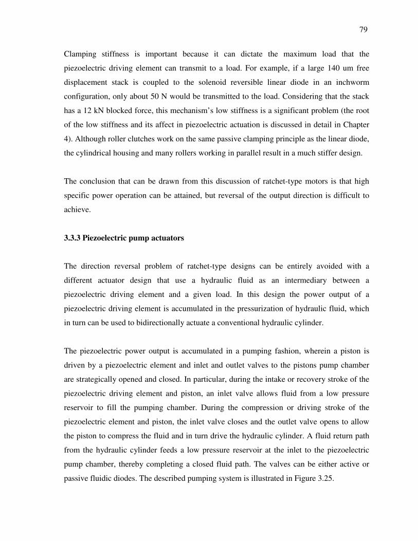
79
Clamping stiffness is important because it can dictate the maximum load that the
piezoelectric driving element can transmit to a load. For example, if a large 140 um free
displacement stack is coupled to the solenoid reversible linear diode in an inchworm
configuration, only about 50 N would be transmitted to the load. Considering that the stack
has a 12 kN blocked force, this mechanism’s low stiffness is a significant problem (the root
of the low stiffness and its affect in piezoelectric actuation is discussed in detail in Chapter
4). Although roller clutches work on the same passive clamping principle as the linear diode,
the cylindrical housing and many rollers working in parallel result in a much stiffer design.
The conclusion that can be drawn from this discussion of ratchet-type motors is that high
specific power operation can be attained, but reversal of the output direction is difficult to
achieve.
3.3.3 Piezoelectric pump actuators
The direction reversal problem of ratchet-type designs can be entirely avoided with a
different actuator design that use a hydraulic fluid as an intermediary between a
piezoelectric driving element and a given load. In this design the power output of a
piezoelectric driving element is accumulated in the pressurization of hydraulic fluid, which
in turn can be used to bidirectionally actuate a conventional hydraulic cylinder.
The piezoelectric power output is accumulated in a pumping fashion, wherein a piston is
driven by a piezoelectric element and inlet and outlet valves to the pistons pump chamber
are strategically opened and closed. In particular, during the intake or recovery stroke of the
piezoelectric driving element and piston, an inlet valve allows fluid from a low pressure
reservoir to fill the pumping chamber. During the compression or driving stroke of the
piezoelectric element and piston, the inlet valve closes and the outlet valve opens to allow
the piston to compress the fluid and in turn drive the hydraulic cylinder. A fluid return path
from the hydraulic cylinder feeds a low pressure reservoir at the inlet to the piezoelectric
pump chamber, thereby completing a closed fluid path. The valves can be either active or
passive fluidic diodes. The described pumping system is illustrated in Figure 3.25.

80
Figure 3.25: Piezoelectric pump concept, Source: Linder 2003
In 1975 Thomas and Bessman conceptualized one of the first piezoelectric pumps. Their
patent proposed using piezoelectric flexural elements to drive a piston and passive valves to
rectify the fluid flow [33]. More recently, Lynch at Georgia Tech has developed a number of
piezoelectric pump designs with reasonable success [34]. His 1999 pump design used a 12”
long piezoelectic stack to drive a hydraulic piston. This design achieved a maximum flow
rate of 750 µl/s at a pressure of 6.1 MPa, which corresponds to a low 5 W power output. The
poor power output was due partly to poor valve dynamics that limited the optimum driving
frequency to 10 Hz. Lynch has continued piezoelectric pump development and his latest
pump design may demonstrate better performance.
CSA Engineering Inc. has also actively pursued piezoelectric pump development. Their
latest pump is shown in Figure 3.26

81
Figure 3.26: CSA’s piezoelectric pump, Source: Linder 2003
The Figure 3.26 pump produced a substantial power output of 42 W at a 400 Hz driving
frequency [35]. CSA has not reported the actuator’s weight; however, based on their
actuator’s design and size its weight can be estimated at about 4 kg. Assuming a 4 kg
weight, the pump’s specific power is approximately 11 W/kg.
Another noteworthy pump actuator is MIT’s miniature piezoelectric pump. The MIT pump
used small single crystal piezoelectric pumping elements and MEMs manufactured passive
valves [36]. MIT’s micro pump is shown in Figure 3.27.

82
Figure 3.27: MIT’s micro piezoelectric pump, Source: Roberts 2002
The MIT design produced a maximum power of 1.6 mW at a 21.6 µl/s flow rate and 300
kPa pressure. Considering that the piezoelectric elements have a cross-sectional are of 1
mm2 the performance achieved by this design is significant.
In the piezoelectric pumps discussed herein, their performance is limited by similar factors
as those of mechanical ratchet-type and inchworm actuators, wherein fluid compressibility,
viscous loses, and dynamic valve response are synonymous to clamp structure stiffness,
mechanical friction, and clamp dynamics, respectively. Another concern with piezoelectric
pumps is fluid cavitation at high driving frequencies, and therefore, piezoelectric pump fluid
systems often require bias pressurization [37].
3.4 EMA vs. Piezoelectric actuators
From the discussions in this chapter it is clear that developing piezoelectric actuators and
motors that simultaneously deliver the high force, but small electric field-induced
piezoelectric strain, to drive loads at high rates is a difficult challenge. Inevitably, inertial
effects, mechanism slop, friction, or structural compliance degrades the power transmitted
between the piezoelectric elements and the output load. Nonetheless, piezoelectric actuators

83
and motors are beginning to compete with electromagnetic actuators in terms of specific
power (EMA are the main competing technology as discussed in Chapter 1). Of the
piezoelectric actuators and motors presented in this chapter, the six best (in terms of specific
power) are compared with EMA feed-screw actuators in Figure 3.28.
Figure 3.28: Specific power comparison of piezoelectric motors and actuators with EMA
Note that although it is typically not fitting to compare both actuators and motors on the
same plot, the purpose of Figure 3.28 is to provide a general evaluation of piezoelectric
actuator and motor technology with respect to conventional EMAs. Also note that in spite
the fact that some of the piezoelectric devices have greater specific powers than EMAs,
there are considerations such as the size of the power electronics and cost that must be
addressed before piezoelectric motors or actuators play a significant role in the actuator
market.
The most obvious observation that can be drawn from Figure 3.28 is that Uchino ultrasonic
motor has the highest specific power of the piezoelectric devices and is far above that of

84
EMAs. Therefore, it would appear that ultrasonic standing wave motors would be the most
attractive design approach. However, as was mentioned in Section 3.2.2, the limited life of
ultrasonic motors is a significant drawback. In addition, Uchino’s motor is a few orders of
magnitude below the size of actuators that are required in aeronautic and space applications
and Uchino’s design is not directly scaleable due to the dynamics nature of its operation. It
is the author’s opinion that quasi-static actuators demonstrate the greatest potential for high
specific power actuation in the 1-100 W power range. Further narrowing the scope of this
dissertation, piezoelectric pumps are not of interest because they face many of the same
maintenance concerns that initiated the recent efforts to move away from hydraulic actuation
systems in aircraft. Therefore, the remaining discussion in this dissertation focuses on
developing a new type of piezoelectric actuator that attempts to combine the best features of
inchworm and ratchet-type actuators while avoiding their drawbacks.

Chapter 4
A NEW PIEZOELECTRIC ACTUATOR
Despite the novel actuator development discussed in Chapter 3, the specific power of state-
of-the-art piezoelectric actuator’s is still a few orders of magnitude below the theoretical
limit discussed in Chapter 1. This chapter takes an in-depth look at why this is the case and,
in particular, the factors limiting quasi-static actuator specific power. This discussion
establishes a foundation for introducing the main topic of this dissertation: an advanced,
high specific power actuator design.
4.1 Improving quasi-static piezoelectric actuators
To discuss the primary factors that limit a quasi-static actuator’s specific power, it is
convenient to describe mechanical power output as the product of work done by a
piezoelectric element over one driving period and the rate at which it is repeated. Both rate
and work are limited by different factors. For example, the rate limit usually involves either
the actuator power electronics, hysteretic self-heating of the piezoelectric material
(discussed in Section 2.3.3) or actuator dynamics. Conversely, the work per driving period is
limited by factors such as friction losses, backlash (slop), and structural compliance.
Compared to the effect of structural compliance, friction losses are generally small while
backlash usually depends on fabrication issues such as machining tolerance, which are not
fundamental to an actuator’s design. Therefore, the effect of structural compliance in
reducing the work per driving period is typically the most important design concern. With
regard to the rate-limiting factors, the driving electronics and the hysteretic heating are
readily managed, while improving the dynamics of the internal components presents a more
significant design challenge. Therefore, the following Sections 4.1.1 and 4.1.2 illustrate the
role played by internal dynamics and structural compliance in limiting quasi-static actuator
mechanical power output.

86
4.1.1 Structural compliance
The influence of structural compliance on quasi-static actuator work output is difficult to
grasp intuitively because the compliant deformation of an actuator’s structure resulting from
piezoelectric actuation is typically on a scale not visible to the human eye. Therefore, in this
section a simple analysis demonstrates how structural compliance can limit the work
transmitted from the piezoelectric driving element to a load.
To begin this discussion, it is useful to review in detail the forces that develop in quasi-static
actuators during a single driving period. To this end, consider the piezoelectric stack coupled
to a generic motion accumulation system in Figure 4.1.
Figure 4.1: Stack driving a generic quasi-static motion accumulator
In this schematic, the motion accumulation mechanism represents a roller clutch in a
ratcheting actuator, an active clamp in an inchworm, or a valve in a piezoelectric pump. The
stack similarly represents a generic driving element. In addition, the load shown in Figure
4.1 represents a torque or pressure load for ratcheting or pump actuators, respectively.
Therefore, the discussion that follows pertains to all quasi-static piezoelectric actuators.
Rigid motion rectification/ accumulation mechanism
Piezoelectric stack
Load

87
The stack’s work delivered to the load can be graphically illustrated by tracing the stack’s
force versus its displacement over a single driving period (electric field-induced actuation
and recoil). Assuming that the load is constant, the linkage between the stack and a motion
accumulation mechanism is rigid, and that the motion accumulation mechanism operates in
an ideal fashion (no backlash and rigid), the stack’s force versus displacement behavior is
given by the plot in Figure 4.2.
Figure 4.2: Piezoelectric stack force versus displacement
At point A, the stack is unloaded and the motion accumulation mechanism supports the load.
As the stack actuates, it unloads the motion accumulation mechanism and builds a force
equal to the load, given by the path from point A to B. When the force on the stack equals
the load, the stack begins to move the constant load; hence, the stack force follows a straight
horizontal path from point B to C. Once the stack reaches its peak displacement at point C,
the motion accumulation mechanism rigidly supports the load, thereby allowing the
unloaded stack to recoil from point D to A.
The net stack work done on the load is graphically shown as the shaded area that the stack’s
force path encloses. Mathematically, the work is given by the integral of the stack’s force
over its driving cycle, which is written as
bF
fδ A
C
D
B

88
b
fLfLL F
PPdPWL δ
δδδ
2
0
−== (4.1)
PL is the constant load and the stack’s displacement at point C (dictated by the load limit line
connecting Fb and f ) is given by
( )bLfL FP−= 1δδ (4.2)
Clearly, the work depends on the magnitude of the load; therefore, the optimum load that
maximizes the work output is of interest. This is easily calculated by taking the derivative of
Equation 4.1 with respect to the load, setting it equal to zero, and solving for the optimum
load. This calculation gives the following
02 =−=b
fLf
L FP
dPdW δ
δ , (4.3)
2bopt FP = and, (4.4)
fbFW δ41
max = (4.5)
For this simple case, Equations 4.4 and 4.5 are intuitive because the rectangular region in
Figure 4.2 is maximum (which is synonymous to work output) for a load that corresponds to
half the stack’s blocked force and a stroke that is half the stack’s free displacement.
If the system’s compliance is considered, the results are less obvious. However, the simple
derivations for the rigid motion accumulation case can be extended to consider a compliant
system. Therefore, consider that a structural compliance, Ceq, exists between ground and the
motion accumulation mechanism, as shown in Figure 4.3.

89
Figure 4.3: Stack driving a compliant generic quasi-static motion accumulator
Following the analysis for the rigid motion accumulator, it is again useful to graphically
illustrate the stack force and corresponding work output, as shown in Figure 4.4.
Figure 4.4: Stack force versus displacement with series compliance
At point A, the structurally compliant motion accumulation mechanism experiences the
entire load. But as the stack extends, the load is transferred from the compliance mechanism
to the stack over the distance prescribed by the compliance deformation at point A.
Therefore, between points A and B’, the force on the stack follows a sloped path governed
by the magnitude of the structural compliance. Once the compliant mechanism becomes
unloaded, the stack force remains constant as it advances the load between points B’ and C.
bF
Motion accumulation structural compliance
fδ A
B’ C
D’
Mechanism structural compliance, Ceq

90
Then, as the stack recoils, the compliance in the motion accumulator allows the load to back
drive the stack to point D’, wherein the compliant mechanism again supports the load. At
this point (D’), the stack continues recoiling unload to its original position at point A.
The work output—graphically shown as the shaded region in Figure 4.4—can be calculated
in a similar fashion to that used for the case of rigid motion accumulation. However, now
the net displacement of the load is not only determined by the load limit line but also the
structural compliance. The net displacement of the load is given by the distance between
points A and D’ or the difference between the displacement given by Equation 4.2 and the
back driven displacement, which is simply the horizontal displacement between points C
and D’. Therefore, by considering the system compliance, the net displacement is given by
eqLLL CP−=′ δδ (4.6)
Following the derivations for the rigid case and substituting the stack’s compliance
( bfEE FKC δ==1 ) in the relations, an optimum load and the corresponding maximum
work output is found to be
( )eqE
fopt CC
P+
=′2
δ (4.7)
( )eqE
f
CCW
+=′
4
2
max
δ (4.8)
Notice that if the compliance Ceq is zero (the structure is rigid), Equation 4.7 and 4.8
simplify to Equations 4.4 and 4.5, respectively. In addition, note that if the generic
equivalent compliance was located between the base of the stack and ground, or between the
top of the stack and the load, the same optimum load and maximum work expressions would
be found. Therefore, Ceq can be thought of as an equivalent compliance that represents the
sum of compliance in series with the piezoelectric driving element.
91
Clearly, increasing the structural compliance or decreasing the structural stiffness in series
with a piezoelectric driving element decreases the net quasi-static work that the a stack can
transmit to a load. However, it is important to clarify that the difference in work output
between the ideal rigid and compliant cases is not lost as heat energy. The examples
considered here were mechanically conservative and the work difference between the rigid
and compliant systems was simply stored as potential energy in the structural compliance.
At this point, little insight can be gained from Equation 4.8 because the equivalent
compliance used in these derivations is completely general. To illustrate more specifically
how structural compliance affects the work output of a quasi-static piezoelectric actuator,
this discussion focuses on the example of a passive clamp (such as the roller clutch).
Passive clamps are composed of wedge element(s) that mate with two angled surfaces to
create a unidirectional locking condition between two surfaces. In this case, the equivalent
compliance involves a component normal to the locking direction and another component
tangent to the locking direction. In the roller clutch, normal compliance represents the radial
stiffness and Hertzian contact stiffness of the roller mating with the wedging surfaces, and
the tangential stiffness represents the torsion stiffness between the clutch housing and
ground. A simplified planar (instead of rotary) passive clamp with the described structural
compliances is shown in Figure 4.5.
Figure 4.5: Compliant passive clamp
PL
FPC
F
Ct
Cn
Rn

92
Although the normal compliance is not directly in series with the load, it adds a crucial
component to the net equivalent compliance of the passive clamp. This is because the force
acting on the normal compliance, due to load PL, is amplified by a factor of αtan1 .
Similarly, the resulting normal compliance deformation seen by the load is amplified by
another factor of αtan1 . Therefore, the equivalent structural compliance of the passive
clamp is given by
α2tannteq CCC += (4.9)
Equation 4.9 can be rewritten in terms of the locking surfaces’ coefficient of friction by
considering the static locking condition that must be satisfied to support the load. The
loading condition is satisfied if the sum of the bias force, FPC, and the maximum friction
holding load, F, is greater than the load, which is given by
LPC PFF ≥+µ (4.10)
Assuming a simple static-Coulomb friction model, the maximum friction force is given
by nc RF µµ = , where αtanLn PR = is the normal clamp reaction force. Note that the
dynamic coefficient of friction (c) is required because the passive clamp must lock under
dynamic operating conditions. Using these substitutions and solving for FPC gives the force
required to maintain a locked condition.
( )αµ tan1 cLPC PF −≥ (4.11)
If Fpc=0 and the locking condition is satisfied, the mechanism is considered to be self-
locking. Typically, in passive clamps the bias force FPC is only intended to position the
wedge and thus, passive clamps are generally designed to be self-locking. Because PL is
positive, the condition required to achieve a self-locking condition is given by
cµα 1tan −≤ (4.12)

93
Using this condition and choosing an angle that meets the self-locking condition and
minimizes the affect of the normal compliance ( cµα =tan ), a new equivalent compliance
can be defined as
2cnteq CCC µ+= (4.13)
This analysis can now be extended to consider a passive clamping quasi-static actuator.
Such an actuator differs from the device shown in Figure 4.3 because two clamping devices
are required to repeat the stack’s driving cycle. Example actuator configurations are shown
in Figure 4.6.
Figure 4.6: Two piezoelectric actuator configurations
For both configurations, the addition of a second compliant motion accumulation
mechanism results in a doubling of the net equivalent structural compliance in the actuator’s
load path. Therefore, the maximum work output of the passive clamp-based actuators shown
in Figure 4.6 is written as
a) b)

94
( ) ( )( )2
22
max 2424 cntE
f
eqE
f
CCCCCW
µδδ
++=
+=′ (4.14)
In a rough example, assuming the tangential and normal compliance to be equal to the stack
compliance (Ct=Cn=CE) and a 0.2 dynamic coefficient of friction, the theoretical work
output of the compliant passive clamp actuator is a factor of 53 lower then a similarly
configured rigid actuator. This particularly impressive result clearly illustrates the
importance of minimizing structural compliance. However, this example exaggerates the
affect of compliance, because passive clamps are typically carefully designed to minimize
the normal and tangential compliances. For example, roller clutches use a rigid cylindrical
structure and multiple roller wedges in parallel.
Nonetheless, compliance is an important concern because the modulus of elasticity of the
piezoceramic (for PZT-5H, 51 GPa) is comparable to that of aluminum. Considering the
simple case in Figure 4.6 a, where an aluminum housing of similar length and cross-
sectional area to the stack is used to support the upper clamp, its equivalent compliance
would, at a minimum, be equal to the stack’s compliance.
Although this discussion has focused on compliance in a passive motion accumulation
device, the general layouts in Figure 4.6 are characteristic of all quasi-static actuators. Thus,
piezoelectric pump performance can be described by the relations in Equation 4.7 and 4.8,
where the equivalent compliance is defined by factors such as fluid compressibility and
valve compliance.
Compliance can also adversely influence other aspects of quasi-static actuator operation.
This is particularly true for inchworm, wherein the work output is not only limited by
structural compliance in series with the load, but also the maximum active clamp holding
load. In accord with the structural compliance analysis in this section, compliance in series
with the active clamps can significantly reduce active clamp holding load. This concern is
one of the motivations for pursuing the rail and micro rigid active clamp designs discussed
in Section 3.3.1.

95
Because the dynamics of the actuator has been ignored thus far, this description of the
interaction between work output and compliance is oversimplified. Nonetheless, this
discussion accurately proposes that the power throughput from the piezoelectric driving
element to the load can be significantly decreased by structural compliances. Therefore, an
important method for improving the power transfer through a piezoelectric actuator is
decreasing compliance in series with the load or the piezoelectric driving element.
4.1.2 Internal actuator dynamics
Section 4.1.1 proposed that the quasi-static actuator power output can be increased by
improving the work output per driving period. This section also discusses increasing quasi-
static actuator power output, but focuses instead on the rate or frequency at which the work
output per driving period can be repeated.
Quasi-static consideration of piezoelectric actuation implies that there is a proportional
relationship between power output and frequency. However, this relationship breaks down at
high frequencies where actuator dynamics is important. Such a break down point or
frequency limit was defined in Section 1.2.2 based on a piezoelectric element’s fundamental
driving frequency. However, in piezoelectric actuators typically other frequency limiting
factors are far below a piezoelectric driving element’s fundamental frequency.
As one might expect, these frequency-limiting factors depend on each actuator’s particular
design, and therefore it is difficult to develop a general frequency limit analysis similar to
that of structural compliance in the previous section. Instead, the PSU stack-driven
piezoelectric motor (previously discussed in Section 3.3.2) is used in this discussion as an
example to illustrate how internal motor dynamics can limit the driving frequency. This
example is then used to formulate general rules for improving internal actuator dynamics.
The PSU stack-driven motor offers insight for this discussion because it demonstrates a
heavily frequency-dependent power output (for details regarding the design and

96
performance of the actuator refer to Section 3.3.2). For example, the motor’s peak power
occurred at 600 Hz while at 900 Hz the power output reduced by a factor of 4. To determine
why this is the case, experimentally measuring the dynamic interactions within the actuator
would have been difficult because the components are packaged compactly. Therefore, a
lumped parameter spring-mass model of the actuator was used to provide valuable insight
into the actuator’s dynamic operation.
The important components of the actuator are represented by the four degree-of-freedom
model in Figure 4.7.
Figure 4.7: Lumped parameter model of the stack-driven roller clutch motor
Simulink was used to numerically simulate the model and the model was in turn verified
with the experimental measured actuator torque versus speed performance data. Simulations
were then performed for 300, 600, and 900 Hz frequencies and a constant 1.0 N-m load. The
resulting time histories for the four degrees-of-freedom in the model are shown in Figure
4.8.
RTL
sm
bm2RIo
2Rkdc
bk
skrsk
sF
2Rcdc
2RIr
2Rkhc
2Rchc
bxsxRrθ
Roθ Output Hub
Rotor Piezo Stack
Stack Base
Holding Roller Clutch
Driving Roller Clutch
R
Stinger

97
Figure 4.8: Simulated time histories at a) 300, b) 600, and c) 900 Hz driving frequencies
In these time histories, the stack extends under its sinusoidal driving excitation to drive the
rotor, but the rotor inertia and stinger stiffness causes it to lag the initial stack motion. As the
rotor follows the stack, the rotor engages the driving roller clutch, thereby causing it to pass
through a small slip or backlash region and lock the output shaft to the rotor. The output
shaft similarly lags the rotor, but then overshoots as its inertia carries it beyond the
amplitude of the periodic rotor motion. The load then causes the output shaft to stop and
back drive through the slip and compliant deformation region of the holding clutch.
Meanwhile, the stack recoils to repeat the cycle.
Clearly, this interaction is dynamic and thus depends on the frequency at which the stack is
driven, thereby describing the difference between the 300, 600, and 900 Hz time histories. In
particular, consider the stack’s amplitude and phase compared to that of the rotor. There is a
resonant motion amplification at the peak power point of 600 Hz. This is illustrated in the
Figure 4.9 amplification factor and phase plots.
-0.2
0.0
0.2
0.4
0.6
0.8
1.0
0.0 0.2 0.4 0.6 0.8 1.0
Time (ms)
Dis
plac
emen
t (m
m)
.
-0.2
0.0
0.2
0.4
0.6
0.8
1.0
0.0 0.2 0.4 0.6 0.8 1.0
Time (ms)D
ispl
acem
ent (
mm
) .
-0.2
0.0
0.2
0.4
0.6
0.8
1.0
0.0 0.2 0.4 0.6 0.8 1.0
Time (ms)
Dis
plac
emen
t (m
m)
.
Base
Stack
Rotor
OutputRrθRoθ
bxsx
a) b) c)

98
Figure 4.9: Simulation rotor-stack motion amplification a) and phase angle b)
It is important to clarify that the stack is not driven at its own internal resonance frequency,
which could result in self-destructive delamitation. Rather, the rotor and stinger are driven in
a resonant single degree-of-freedom base excitation mode. As defined by the motor
dynamics, the 600 Hz frequency represents the approximate upper frequency bound within
which the actuator can operate, because above 600 Hz the rotor motion is attenuated. To
increase the frequency bound defined by the rotor-stinger resonance, either the stiffness of
the stinger must be increased or the rotor mass must be decreased. However, decreasing the
mass of the rotor could affect its stiffness and increasing the stiffness of the stinger would
likely involve increasing its mass. Therefore, increasing the frequency bound is a difficult
design challenge. Complicating things further, the actuator stiffness can influence the work
output per driving period, as discussed in the previous section. The obvious conclusion that
can be drawn from this example is that components transmitting force between the
piezoelectric driving element and the load should be designed to have high stiffness and low
mass.
0.0
0.5
1.0
1.5
2.0
2.5
200 300 400 500 600 700 800 900 1000
Frequency (Hz)
Mot
ion
Am
plifi
catio
n R
atio
.
0
30
60
90
120
150
180
200 300 400 500 600 700 800 900 1000
Frequency (Hz)
Pha
se A
ngle
(deg
rees
) .
a)
b)

99
As a general guide, optimally designed actuator components that minimize structural
compliance while also minimizing mass will generally have uniform distributions of stress
throughout their structures. This statement is, of course, true for most engineering structural
design.
A less obvious method for achieving high stiffness and low mass components for any given
design is to fabricate the actuator components using materials with a high stiffness to weight
ratio. Interestingly, high-grade titanium, steel, and aluminum have similar specific moduli or
ratios of their modulus of elasticities to density (approximately 25 MPa-m3/kg). Even so, a
much less common material, beryllium, has an impressive 160 MPa-m3/kg specific modulus.
Pure beryllium has the highest specific modulus of all metals. However, it is brittle and
therefore typically alloyed with aluminum to improve its machining characteristics.
Aluminum-beryllium alloys have a specific modulus of about 91 or 3.6 times that of steel. In
the stack-driven motor, if the original steel rotor and stinger were replaced with aluminum-
beryllium alloy, the frequency bound could hypothetically be doubled
( eqeqeqeq mkmk 9.16.3 ≈≈ω ).
The drawback of beryllium is the health risk it poses. Inhalation of airborne beryllium
partials causes a serious lung disorder. If beryllium actuator components were used in an
actuator, they would need to be handled in a special fashion and for most applications this
requirement is unacceptable. Nonetheless, beryllium is currently being used in some space
and aeronautics applications.
The nontoxic and more commonly used aluminum-lithium alloy has shown to be 5% lighter
and 7% stiffer than conventional aluminum alloys [38]. Lockheed is currently using
aluminum-lithium alloy for some military fighter bulkheads.
4.2 A new quasi-static piezoelectric actuator
Based on the ideas in the previous section, the two most important design objectives for
developing a high specific power quasi-static actuator are minimizing structural compliance

100
and improving the actuator’s internal dynamic frequency bound. This section presents a new
quasi-static actuator design that attempts to addresses these two design objectives. The new
actuator design discussed in this section is significant because it establishes this dissertation
as an original and significant contribution to piezoelectric actuator research.
4.2.1 Hybrid actuator concept
In its most basic form, the new actuator consists of a piezoelectric stack (driving element)
sandwiched between an upper holding clamp and a lower driving clamp, as is the case for
conventional inchworm actuators. This new actuator design is shown in Figure 4.10.
Figure 4.10: New actuator design
The new actuator also uses a motion accumulation principle similar to that of inchworm,
where electric field-induced strain from a stack is periodically accumulated by intermittently
locking and releasing holding and driving clamps. The holding clamp restrains the load
while the stack is recoiling and the driving clamp supports the base of the stack while it
advances the load. Therefore, the load is repeatedly stepped forward in correspondence with
the periodic excitation of the piezoelectric element. An example stepping sequence for a
single driving period of the stack is shown in Figure 4.11.
Piezoelectric stack
Holding clamp
Locking wedge
Load
Driving clamp

101
Figure 4.11: Quasi-static motion accumulation stepping sequence
Clearly, periodic repetition of this sequence leads to a continuous stepping motion.
4.2.2 The hybrid clamp
The essence of the new actuator is the wedge clamp configuration shown in Figure 4.12.
Figure 4.12: New hybrid clamp
Although simple, the wedge clamp is unique and significant because it combines the
reversibility and low compliance of inchworm active clamps with the simplicity and quick
response of ratcheting-type passive clamps, thereby acting as a hybrid passive/active clamp.
(1) Stack extends (2) Holding wedges move inward
(3) Stack recoils (4) Driving wedges move inward
Load Bias forces
PL
FHC
F
Rn

102
For the hybrid clamp to hold a load, a similar locking condition to that of the passive clamp
must be satisfied; this locking condition is given by
αµ tanLHC PFF ≥+ (4.15)
In Equation 4.15, the maximum friction force is defined as LcPF µµ = , giving the following
expression.
( )cLHC PF µα −≥ tan (4.16)
For the self-locking condition to exist ( 0=HCF ), the following must be satisfied.
cµα 1tan −≤ (4.17)
Notice that this is the same result found for the passive clamp. However, an important
distinction between the hybrid and passive clamps lies in the difference in their equivalent
structural compliance expressions. In the case of the hybrid clamp, the influence of the
normal compliance shown in Figure 4.13 is reduced by a factor tan2 instead of being
amplified by a α2tan1 factor, as was the case for the passive clamp.
Figure 4.13: Hybrid clamp with structural compliance
PL
Ct
Cn

103
This gives an equivalent structural compliance of
α2tannteq CCC += (4.18)
Considering the optimum self-locking condition ( cµα =tan ), the maximum work output of
the hybrid clamp actuator is written as
( ) ( )( )2
22
max 2424 cntE
f
eqE
f
CCCCCW
µδδ
++=
+=′ (4.19)
If a similar example scenario to the passive clamp is assumed, wherein the tangential and the
normal compliances are equal to the stack compliance (Ct=Cn=CE) and the dynamic
coefficient of friction is 0.2, the theoretical work output of the compliant hybrid actuator
relative to the ideal rigid actuator is only decreased by a factor of 3.1. This is an impressive
result compared to the factor of 53 reduction for the passive clamp actuator.
Another way to view this difference between the hybrid and passive clamp is that the
internal reaction forces in the hybrid clamp for a given load are smaller than passive clamp
forces. Therefore, smaller clamping elements can be used to hold the same load. Smaller and
lower mass clamping elements can also increase the dynamic frequency bound for the
actuator. This, in turn, implies that the actuator can be driven at a high frequency to achieve
high power outputs. Therefore, in theory, the hybrid clamp should have a low compliance
and good frequency response relative to the passive clamp.
Compared to the active clamp, the hybrid clamp’s primary benefits lie in its self-locking
capability and simpler power electronics. The passive self-locking condition of the hybrid
clamp can hypothetically support an infinite load. Therefore, in a piezoelectric actuator, the
hybrid clamp structural compliance is important rather than the maximum clamping load, as
is the case for active clamps. With regard to the power electronics, the hybrid clamp only
requires a reversible bias force, while active clamps require high frequency power

104
electronics to operate. Typically, active clamping actuators therefore require triple the power
electronics of a hybrid clamping actuator with similar piezoelectric driving element.
In theory, the hybrid clamp actuator has significant advantages over other quasi-static
actuators. However, practical implementation of the hybrid clamp is a challenge. In
particular, reliable reversibility—and more notably, four-quadrant operation—is difficult to
achieve. These issues are considered next.
4.2.3 Four-quadrant operation
Four-quadrant operation refers to an actuator’s ability to bidirectionally drive a load that
either opposes the actuation direction or has the same sense. These combinations of load and
actuation direction are shown in Figure 4.14.
Figure 4.14: Four-quadrants of actuator operation
Consider achieving second quadrant operation by simply reversing the bias force on the
wedges. Ideally, the direct inverse of the first quadrant stepping sequence—previously
illustrated in Figure 4.11—would give a downward motion as shown in Figure 4.15.
(1) (2)
(3) (4)
Motion Load Motion Load
Motion Load Motion Load

105
Figure 4.15: Stepping sequence when the directions of the intended motion and load have the same sense
However, in this sequence, the outward wedge movement must be precisely controlled to
achieve downward stepping. If, for example, the holding wedges in Figure 4.15, frame (2)
moves too far outward—greater than the ratio of the stack’s step size and the tangent of the
wedge angle ( αδδ tanstackwedge > )—the stack recoiling in frame (3) would not release the
load on the driving wedges. This is shown in Figure 4.16.
Figure 4.16: Actuator stall resulting from upper wedges stepping too far
Further complicating the issue, the size of the outward steps depends on the stack’s step size
and, in turn, the load (recalling Equation 4.2).
(1) Stack extends (2) Holding wedges move outward
(3) Stack recoils (4) Driving wedges still support load
Load Intended Motion
(1) Stack extends (2) Holding wedges move outward
(3) Stack recoils (4) Driving wedges move outward
Load Intended Motion

106
To avoid the requirement of a control system for managing the wedge movement, the bias
force must be large enough to overcome the static friction forces holding the wedge.
However, recall that the bias force must also satisfy the dynamic locking condition for
proper first quadrant operation (given by Equation 4.16). In other words, from a resting
position, the bias force must be large enough to push the wedge out of its self-locking
condition, and during dynamic operation, the bias force must also prevent the wedge from
slipping. Assuming a static-Coulomb friction model, wherein static surface coefficient of
friction is greater than that of sliding surfaces, the minimum bias force required to satisfy
these conditions poses a concern, because in the initial actuation concept small bias forces
were only intended to position the wedges.
To determine the magnitude of the bias force that is required to achieving first and second
quadrant operation, consider Figure 4.17.
Figure 4.17: Forces in hybrid clamp
The bias force required to satisfy these two conditions can be found by considering the first
quadrant dynamic clamp condition given by (previously developed in Section 4.2.2)
PL
R1
R3
FHC-R
R2
Fs
PL
R1
R3
FHC-F
R2
Fc
a) First quadrant operation
PL
R1
R3
FHC-F
R2
Fc
PL
R1
R3
FHC-R
R2
Fs
b) Second quadrant (reverse) operation
Intended Motion
Intended Motion

107
cL
FHC
PF µα −≥− tan (4.20)
The complementary condition for second quadrant operation is given by
s
FRF RHC µ≥+− 1 (4.21)
Rearranging Equation 4.21 and using the fact that αtan1 LPR = and Ls PFs
µµ = , it can be
rewritten as
αµ tan−≥−s
L
RHC
PF
(4.22)
Plotting the ratio of the bias force and load in Equations 4.20 and 4.22 for various friction
coefficients and clamp angles gives the following
Figure 4.18: Design region of bias force and wedge angles whereby both first and second
quadrant operation are achievable
0
0.02
0.04
0.06
0.08
0.1
6 8 10 12 14 16
Angle (degrees)
L
HC
PF
2.0=cµ18.=cµFor locking when moving forward For sliding in reversing
2.0=sµ 22.=sµ
0.01
0.02
0.03
0.04
0.05

108
The shaded regions in Figure 4.18 represent the design space wherein both Equations 4.20
and 4.22 are satisfied. The angle that minimizes the bias force lies at the intersection of the
dashed lines. Therefore, equating the right-hand sides of Equations 4.20 and 4.22 and
solving for the optimum wedge angle gives
+= −
2tan 1 cs
opt
µµα (4.23)
The corresponding ratio of the bias force and load is given as
2
tanmin
cscopt
L
HC
PF µµµα −
=−=
(4.24)
Notice that if the static and Coulomb coefficients of friction are equal, the minimum bias
force required to achieve both first and second quadrant operation is zero, but if the static
and Coulomb coefficients are 22.0=sµ and 18.0=cµ , respectively, the minimum bias
force is approximately 2% of the actuation load. If a constant bias force is assumed over the
wedge displacement, the quasi-static work required to move both wedges compared to that
of the load for a single driving period is given by
αδ
δδ
αδδ
tan22
0
tan/
0
==
=
L
HC
L
HC
load
wedge
PF
dP
dF
W
Wload
loadwedge
(4.25)
For this example case ( 18.0=cµ and 22.0=sµ ), the work required to move the wedges is
20% of that required to move the load. This implies that a substantial parasitic power input
to the actuator is required to achieve first and second quadrant operation. However, in
theory, the bias force is only required for the instant of time when the wedge is locking or
when it is breaking the wedge free from the static locked condition. Therefore, the actual
work required to move the wedge is likely to be lower than what is given by Equation 4.25.
In further support of this argument, stack actuation can vary the load on the wedges, which

109
in turn would reduce the required bias force. Nevertheless, the conclusion that can be drawn
from this analysis is that first and second quadrant operation can be achieved with the hybrid
clamp, but care should be taken to properly design the angle so it minimizes the required
bias force.
Thus far, only the first and second quadrant operation has been discussed. However,
assuming symmetry of the hybrid clamping mechanism, it follows that operation in
quadrants (3) and (4) is also achievable. An example symmetric clamp design achieving
four-quadrant operation is shown in Figure 4.18.
Figure 4.19: Hybrid actuator design capable of achieving four-quadrant operation
In summary, this section has presented an original hybrid clamp that is self-locking, has low
structural compliance, can be designed to have a high frequency bound, and can achieve
four-quadrant operation.
Load
or load
Wedges

110
4.2.4 The improved feed-screw design
One major drawback of the initial hybrid design is that the actuator’s width (horizontal
dimension in Figure 4.10), must be a factor of αtan2 greater than the actuator’s maximum
stroke. For an actuator with a 5 cm stroke and 10 deg wedge angle, the actuator would
require a large width of 57 cm. However, this issue can be addressed with a new helical
(hybrid) actuator configuration. A cross-sectional view of the helical or feed-screw actuator
design is shown in Figure 4.20.
Figure 4.20: Feed-screw actuator design
In this new design, the nuts are constrained axially, but allowed to rotate on the feed-screw.
The feed-screw is constrained in rotation, but free in translation. The surfaces that constrain
the nuts axially are analogous to the lower horizontal surface of the initial wedge angle and
the screw is analogous to the wedge angle surfaces. Therefore, in the helical design, rotation
Bias Torque
(a) Initial hybrid design (b) Feed-screw design

111
of the nuts has an affect similar to that of translation of the wedge in the initial planar
design.
The helical concept is significant because it wraps a long wedge compactly into the hybrid
actuator design. In addition, the helical design requires a bias torque instead of a bias force,
and thus, this feed-screw design is conducive to using a conventional electric motor to apply
a bias torque. The advantage of using an electric motor is the ease of reversing the bias
torque direction to achieve four-quadrant operation.
4.3 Concept originality
In 2002, a research group in Singapore published a paper that describes a similar actuator
concept to the hybrid actuator [39]. Their design used the same wedge clamp concept as the
design presented in Figure 4.10. In their prototype, large flat wedging components at either
end of a small stack (20 mm length) were used. Their prototype is shown in Figure 4.21.
Figure 4.21: Hybrid actuator prototype published in 2002 by Singapore research group

112
An 1176 N blocked force was achieved with the prototype in Figure 4.21. Other data such as
actuator speed and stack driving frequency data were not reported. Their design focus was
precision positioning and control—not high specific power. The Singapore group also
proposed using a helical wedging concept similar to the hybrid feed-screw prototype.
However, their published research work has not yet addressed the complications of
implementing four-quadrant operation.
Despite the Singapore group’s publication, the work presented in this dissertation began
coincidentally in early 2002 as an original idea and is currently more advanced than the
Singapore group’s work. Therefore, this dissertation claims equal credit for the original
development and demonstration of the hybrid clamp based actuator.

Chapter 5
EXPERIMENTAL FEED-SCREW ACTUATOR DEVELOPMENT
In most cases, conceptual piezoelectric actuator development carries little significance until
having met with experimental success. Hence, this chapter presents a thorough experimental
demonstration of the feed-screw piezoelectric actuator proposed in Chapter 4. This actuator
development involved an iterative process in which three proof-of-concept actuators were
fabricated and tested. The knowledge gained from these initial prototypes culminated in a
successful, fully functional actuator [40]. The experimental work described in this chapter
and the analytical actuator developments in Chapter 4 were conducted simultaneously but,
for presentation purposes, it is convenient to discuss them in separate chapters.
5.1 Hybrid actuator prototypes
5.1.1 Initial proof-of-concept prototype
The first of the three proof-of-concept actuators initiated interest in the simple and compact
hybrid clamp by demonstrating its potential for quasi-static piezoelectric actuation. It used a
planar wedge configuration and was powered by a small co-fired piezoelectric stack, having
a 3 kN blocked force and 18 µm free displacement. The stack was sandwiched between two
angled blocks, and four rollers were used as wedge clamping elements. Small springs
applied bias forces to the wedges, thereby mating the rollers with the angled blocks and
another set of rigid support surfaces. Because the bias force was applied by unidirectional
spring loads, this proof-of-concept design was only intended to demonstrate first quadrant
operation. The described actuator is pictured in Figure 5.1 (the bias force springs connecting
the roller are not shown in Figure 5.1).

114
Figure 5.1: Initial hybrid actuator prototype
Weights were hung from the upper angled block to load the actuator. For a set of constant
loads, the actuator’s average speed was measured using a manual timing method. The
actuator was tested at 10, 50, 100, 200, and 500 Hz drive frequencies, giving the load and
power versus speed performance shown in Figure 5.2.
Piezoelectric stack
Roller wedges
Load

115
Figure 5.2: Torque a) and power b) versus speed performance plots
A maximum power output of 0.2 W was achieved at the peak 500 Hz driving frequency. At
the optimum 500 Hz frequency, the actuator demonstrated a 6 mm/s maximum speed and a
90 N blocked force. Although the 0.2 W power output of this actuator is not particularly
impressive, the simple actuator design provided evidence supporting the potential of the
hybrid clamp.
5.1.2 Feed-screw prototype
The next proof-of-concept actuator was designed to demonstrate the helical feed-screw
actuator concept. The feed-screw actuator’s helical clamp design consisted of two
conventional bronze nuts and corresponding standard ACME screws. The nuts were
0
20
40
60
80
100
0 1 2 3 4 5 6 7
10 Hz50 Hz
100 Hz200 Hz500 Hz
Speed
L
oad
(N)
0.00
0.04
0.08
0.12
0.16
0.20
0 1 2 3 4 5 6 7
10 Hz
50 Hz
100 Hz
200 Hz
500 Hz
Po
wer
(W)
b)
a)

116
constrained axially in a cylindrical actuator housing and the screws mounted directly to
either end of stack having a 3 kN blocked force and 54 µm free displacement. Small
electromagnetic motors turned worm gears, meshing with spur gears on the nuts to apply
bias torque to the nuts. The initial feed-screw prototype (excluding the electromagnetic bias
motors) is shown in Figure 5.3.
Figure 5.3: Unsuccessful initial feed-screw piezoelectric actuator
This actuator prototype was unsuccessful: It demonstrated a disappointingly low force and
slow motion, and failed to achieve reliable reversibility. Due to the compact nature of the
actuator’s design, the root of its poor performance was difficult to determine. It was
hypothesized to be related to nut binding, resulting from lack of sufficient nut and screw
bearing support.
5.1.3 Ball screw prototype
In an effort to prevent nut binding, the third prototype was designed with ball screws instead
of conventional ACME feed-screws. Ball screws consist of a set of recirculating ball
bearings located between the nut and screw threads. In addition, the new prototype used a
Nuts and spur gears
Stack Screw output

117
significantly more exposed and experimentally-conducive layout in response to the
problems with the more compact previous prototype. The ball screw actuator used a large
stack (140 µm free displacement and 12 kN blocked force) to power the actuator. In a
manner similar to that of the first feed-screw prototype, small electromagnetic bias motors
drove worm gears that meshed with spur gears on the nuts. A stiff compression spring was
used to provide an actuation load, as shown in the Figure 5.4 test setup.
Figure 5.4: Ball screw prototype actuator
Ball screw nut Frictional locking surfaces
Spring load Bias torque motor
Stack
118
The ball screw actuator performed well, producing an 1870 N blocked force and 0.7 mm/s
free speed. The 1870 N blocked actuation force is an impressive 25% of the stack’s blocked
force. However, because the actuator’s performance peaked at a low 5 Hz driving frequency,
the actuator’s 0.7 mm/s maximum speed is unacceptably slow. Above the 5 Hz driving
frequency, the nuts could not step quick enough to accumulate the stack’s motion. The poor
dynamic response of the nuts was due to their large rotary inertia and the small
electromagnetic motor’s bias torque. This was an important observation that reinforced the
conclusions discussed in Section 4.1.2 with regard to the dynamic frequency limit in quasi-
static actuators.
Because the electromagnetic bias torque was small and the wedge angle (screw pitch angle)
was not (at this point) designed according to the discussion in Section 4.2.3, second quadrant
operation (reversal under an aiding load) was not achieved with the ball screw actuator. In
the next iteration of actuator development, prime consideration was given to include second
quadrant operation by properly designing the screw pitch angle and the bias torque motor,
while also minimizing the nut inertia.
5.2 Development of a new feed-screw actuator
With knowledge gained from the first three prototypes, the feed-screw design was poised for
implementation as a full-fledged application-based actuator. Coincidentally, a DARPA-
funded program at the Lockheed Martin Corporation was seeking new piezoelectric actuator
technology for their Morphing Aircraft Structures (MAS) project. Collaboration between the
Center for Acoustics and Vibration (CAV), KCF Technologies (led by former CAV student
Dr. Jeremy Frank), and MPC Products in Chicago provided the means for applying the feed-
screw piezoelectric actuator in the Lockheed’s MAS project. The subsequent evolution of
the feed-screw actuator from experimental prototype to robust actuator involved a close
working relationship between the CAV and KCF Technologies.

119
5.2.1 Lockheed’s Leading Edge Flap application
Lockheed’s MAS project involved changing the wingspan of a small unmanned combat
aircraft vehicle (UCAV) to adapt to different flight conditions [40]. The aircraft morphing
involved changing the wing’s shape to optimally accommodate a fuel efficient “cruise”
configuration for long flight missions and a second high speed and maneuverable “dash”
configuration. Lockheed’s concept for changing the UCAV’s wing area involved folding
part of the wings inboard—in a similar fashion to the way birds tuck their wings when
diving for prey. This folding wing concept is shown in Figure 5.5.
Figure 5.5: Lockheed morphing wing concept, Source: Love 2004
Lockheed’s morphing UCAV concept has a delta shaped wing with pivots located at mid-
span and at the root of the wings. A single jet engine is located at the center of the aircraft
fuselage. A schematic of the basic Lockheed folding wing aircraft structure is shown in
Figure 5.6.

120
Figure 5.6: Structural design of the folding wing UCAV, Source: Love 2004
The first phase of the Lockheed MAS project involved demonstrating the folding wing
concept with in a ¼ scale remote control (RC) model aircraft. Lockheed’s RC model was
completed in May 2004 and is presently undergoing flight testing. The model has a small jet
engine and uses electromagnetic servo actuators to fold the wings. Lockheed’s RC model is
intended to fly upwards of ~140 mph and fold its wings during flight. A recent photo of the
model aircraft is shown in Figure 5.7.

121
Figure 5.7: Lockheed’s ¼ scale remote control model of the morphing UCAV, Source: Love 2004
Although a full-scale folding wing UCAV is a few years off, the initial part of the Lockheed
project involved the development of key technology such as actuators to fold the wings. The
power requirement for folding the wings during flight is in the kilowatt range; therefore,
large electro-hydraulic actuators (EHA) or an air loading configuration appear to be the best
actuation technology for the wing-fold application. However, there are other relevant
actuator applications. One application involves actuating a leading edge flap (LEF) that
covers gaps between the fuselage and the inboard section of the UCAV’s folded wings.
Because it has a passive rigid and locked failure mode, a high force output at low speeds,
and a compact cylindrical design, the feed-screw piezoelectric actuator is potentially an ideal
candidate for actuating the LEF.
Actuating the LEF involves rotating it against a 6100 in-lb combined air and weight load.
Under this load condition, the flap must rotate a maximum travel of 15 deg at a nominal rate
of 15 deg/s. The flap loading is unidirectional and, thus, only first and second quadrant

122
actuation is required. In addition, the flap actuators must fit in a 20 x 33.7 x 3.0 in design
space located within the flap. Finally, the actuator must withstand loads up to twice the rated
6100 in-lb load. The actuator’s electromechanical efficiency was not a primary concern in
the first phase of the actuator development. Also, note that, to conform to Lockheed’s
measurements, the English system of units was reluctantly adopted. Henceforth, in the
remaining LEF discussions, English units are intermixed with SI units.
5.2.2 Feed-screw actuators for achieving the LEF requirements
Next, the design of a linkage and feed-screw piezoelectric actuator capable of meeting the
LEF actuation requirements was pursued. Using a simple dynamic model to estimate the
size and force versus speed capability of the feed-screw actuator, five actuators were placed
in parallel driving a simple 1.0 in long lever arm to achieve the LEF actuation requirements.
An illustration of the proposed actuators in the flap’s design envelope is shown in Figure
5.8.
Figure 5.8: The leading edge flap design envelope and the proposed integration of five piezoelectric feed-screw actuators
33.7 in
20.0 in
3.0

123
To meet the LEF actuator requirements, each actuator must produce 1220 lbs of force at a
rate of 0.26 in/s. Based on the model predictions, the following estimated force versus speed
performance for each actuator was expected.
Figure 5.9: Model speed versus load performance predictions for feed-screw actuator
The model used for these actuator predictions is not discussed here because it was the basis
for a more comprehensive actuator model that is described in detail in Chapter 6.
5.2.3 LEF feed-screw actuator design
In an effort to make the feed-screw actuator compact and robust, a new LEF actuator layout
differing from the initial prototypes was adopted. The primary innovation in the new LEF
feed-screw actuator design was the use of a single hollow electromagnetic bias torque motor
located directly between a holding and driving nut. In this new design, the motor was
LEF Requirement: 0.26 in/s, 1220 lbs

124
connected to the nuts through two torsion springs located at either end of the motor rotor.
These flexible spring couplings allowed the nuts to step forward independently. An
additional benefit of this nut and motor configuration is that the nuts were much closer
together than in previous designs, where the nuts were located at either end of the stack. The
close proximity of the nuts minimizes the structural compliances in series with the stack (see
Section 4.1.1 for an in-depth discussion of the effect of structural compliance on actuator
performance). In addition to the new motor configuration, a hollow stack was used to
accommodate the screw stroke in a compact configuration. A drawing of the described
actuator design is shown in Figure 5.10 (a complete set of drawings are provided in
Appendix A).

125
Figure 5.10: Cross-section of LEF feed-screw actuator design
Upper holding nut
Lower driving nut
EM motor rotor Motor ball bearings EM motor stator
Torsion spring couplers
Top cap
Nut support plate
Actuator housing
Stack cap
EM motor encoder
Stack
Screw
Ball spline
Bottom cap
Output
Ground

126
The operation of this new feed-screw design is based on a principle similar to that used in
the past prototype actuators, wherein the stack is driven periodically and the two nuts are
intermittently rotated to accumulate the stack’s motion. Thus, while extending, the stack
pushes on the lower (driving) nut to drive the loaded screw, during which time the upper nut
is rotated (without translating) by the bias motor to track the screw motion. As the stack
relaxes, the upper (holding) nut holds the screw and prevents it from back-driving with the
stack. This allows the lower nut to rotate and track the stack recoil. In this way, the nuts step
intermittently forward as the bias torque motor alternately loads the torsion coupling springs.
In this way, the torque motor follows a nearly constant rotational velocity as it steps the
nuts.
Design of the LEF feed-screw piezoelectric actuator components began with the feed-screw
and the nuts. To minimize wear and maintain consistent surface friction, lubrication between
the screw and nuts was important. However, because the clamping behavior of the hybrid
screw-nut combination is independent of the free-play between the threads, screw and nut
wear will not decrease the force or speed performance of the feed-screw actuator (although
wear can increase the slop between the actuator output and ground).
According to Marks’ Standard Handbook, hardened precision ground and grease-lubricated
steel surfaces have static and Coulomb friction coefficients of 0.15 and 0.08, respectively
[41]. Assuming these coefficients of friction and following the self-locking analysis
described in Section 4.2.3, an optimum pitch angle of 6.5 deg is found. Based on the 1220 lb
actuation load, a 2.0 factor of safety, and the rated load range of typical steel ACME screws,
a 0.75 in outside diameter screw was selected for the actuator [42]. The standard thread pitch
for a 0.75 in ACME screw that most closely matches the desired 6.5 deg angle is a 5.8 deg
thread pitch angle, which corresponds to a 5 threads per inch screw (0.630 in pitch
diameter). Based on the nominal 1220 lb actuation load and the screw’s surface friction, a
predicted short duration bias torque of 2.1 N-m would be required to break the nuts free and
achieve second quadrant operation.

127
At this point in the project, demonstrating first quadrant actuation was of utmost importance.
Thus, uncertainty in the coefficient of friction and the effect of actuation dynamics on the
simple models used to predict the optimum pitch angle led to a design that ensured the self-
locking condition rather than one that would ensure second quadrant operation. This
conservative design involved using precision ground ACME feed-screws rather than a ball
screw. In the case that first quadrant operation work well but second quadrant operation is
not achieved, roller thrust bearings could be easily integrated into the actuator to revert it to
the original configuration (which in fact turned out to be necessary as will be discussed in
Section 5.3).
In this actuator configuration, the torque required to step the nuts is significant because
during each driving period of the stack the nuts are required to accelerate from rest to a new
position and then come abruptly to a stop and support the load. For the actuator to operate at
high frequencies, the bias motor torque must be large enough (and the nuts must have a low
enough rotary inertia) that the nuts can accelerate quickly. Using preliminary model
predictions, a continuous 1.0 N-m bias torque was determined to be sufficient to
dynamically step reasonably-sized nuts at a 100 Hz frequency.
Operating at a 100 Hz frequency, a stack having a 20 kN blocked force and 200 µm free
displacement was estimated to suitably achieve the 0.26 in/s and 1220 lb design point. There
are a number of companies that fabricate hollow cylindrical stacks capable of achieving the
described performance. However, a small, Munich-based company, Piezomechanik Gmbh,
uses unique compact plate-through electrode connectors, giving the stack a compact design.
Piezomechanik stacks have a special pre-compression casing that protects the stack from
tensile and bending loads. The Piezomechanik stack selected for the feed-screw actuator is
shown in Figure 5.11.

128
Figure 5.11: Piezomechanik cylindrical piezoelectric stack actuator
The stack shown in Figure 5.11 has a 45 mm outside diameter, 25 mm inside diameter, and
200 mm length. Driving the stack unipolarly to 1000 Vpp, the stack and pre-compression
housing achieved the required 20 kN blocked force and 200 µm free displacement. Driving
the stack bipolarly from –200 to 1000 Vpp gives an even larger 260um free displacement.
The stack layers are 1.0 mm thick; therefore, at the maximum bipolar voltage, the
piezoceramic experiences a large 1200 V/mm electric field. The stack uses a variant on the
soft PZT-5H piezoceramic and has a large 4.2 F capacitance. The stack’s fundamental
extensional resonance frequency of 4 kHz is well above the actuator’s intended 100 Hz
driving frequency.
A custom power supply was developed by Qortek to power the stack. Qortek’s power supply
was designed to produce a 50-100 Hz variable frequency and fixed –200 to 1000 Vpp bipolar
voltage output. For experimental purposes, it would have been useful to have a higher
frequency band and variable voltage output; however, budgetary and time constraints
limited the power supply to the described subpar design and size. The Qortek power supply
is shown in Figure 5.12.

129
Figure 5.12: Qortek power supply for driving Piezomechanik stack
The bias motor requirements were unique in that the motor needed to produce a minimum
2.1 N-m instantaneous and 1.0 N-m continuous torque over the low speed 0-200 rpm range.
In addition, it must have a small torque detent (‘detent’ refers to fluctuation in torque during
rotation, typically due to the orientation of the magnet poles) and produce a steady state
torque at stall. The motor geometry requirements are also unique in that the screw must pass
freely through the rotor’s center axis. An ideal motor for this application was a frameless
brushless DC motor produced by the Bayside Motion Group. The Bayside motor, with
custom fabricated bearing sleeves, is pictured in Figure 5.13.

130
Figure 5.13: Bayside bias torque motor and custom fabricated bearing support bushings
The Bayside motor has a simple construction with eight electromagnetic coil polls on an
outer stationary stator. Eight corresponding rare-earth permanent magnet polls are mounted
to a hollow inner rotor. The motor has a 0.15 N-m/W torque constant, 1200 rpm peak speed,
2 N-m intermittent stall torque, and 1 N-m continuous stall torque (100% duty cycle).
Motor commutation for the Bayside motor could have been achieved using Hall sensors or
other means, but the precise position feedback and small size of an optical encoder made it
the ideal commutation option. An optical encoder consisting of a rotor disc and an optical
pickup head from US Digital was used for the Bayside motor.

131
Figure 5.14: US Digital optical encoder disc and head
The US Digital encoder works by emitting light on one side of the disc while two slightly
offset light sensitive transducers respond to the light projected through the translucent slits
in the disc: The two electrical signals from the transducers are conditioned and compared to
provide relative rotor position feedback. This feedback is fed to the motor controller, which
controls the power supplied to the motor’s electromagnets. The generic Bayside motor
controller and power supply used to drive the bias motor is shown in Figure 5.15.
132
Figure 5.15: Bayside standard brushless DC motor controller
Designing the torsion spring couplers that join the motor rotor and nuts presented another
challenge. The torsion springs needed to have a large torsion spring constant, handle large
torsion displacements, fit into a small space, and be compliant in the longitudinal direction
(to allow the nuts to move easily as the stack is actuated). To meet these requirements,
titanium alloy was the ideal spring material because it can accommodate high strain energy
and high stress levels before yielding. The obvious design for meeting the described
requirements is a multi-start helical spring. However, helical cuts are difficult to fabricate
and due to cost and time constraints, a variant on the helical spring design was fabricated.
The torsion stiffness of the springs was designed such that the 1 N-m torque of the bias
motor would deform the spring an angle corresponding to a linear nut translation equal to
the 260 µm maximum stack free-displacement, giving a 3.1 N-m/rad torsion stiffness.
With regard to the overall actuator design, two general design objectives were sought. The
first objective was to maintain alignment between each of the components in an effort to

133
prevent nut binding and ensure that contact between the nuts and their mating surfaces was
flat and rigid. Therefore, close-fitting alignment features were added to each of the mating
components. The second objective was to minimize actuator structural compliance by
creating the most direct load path from the nuts to ground. Therefore the number of mating
part interfaces were kept to a minimum.
5.2.4 Fabrication and assembly of the LEF actuator
MPC Products specializes in flight control systems and electromagnetic feed-screw
actuators, and thus, their expertise was particularly useful for manufacturing the precision
actuator components. MPC custom-fabricated the screw and nut to unusually precise
tolerances (~20 m clearance between nut and screw) to avoid the sticking and
misalignment problems encountered with the first feed-screw prototype. The actuator
housing, bottom cap, nut support plate, top cap, stack cap, and rotor bearing supports (all
labeled in Figure 5.16) were also manufactured at MPC.

134
Figure 5.16: Feed-screw actuator assembly
Upper holding nut
Lower driving nut
EM motor
Top cap
Nut support plate
Actuator housing Stack cap
Stack
Screw
Bottom cap

135
Because the stack cap, nut support plate, screw, and nuts could potentially wear from
experiencing intermittent contact with one other, they were fabricated from high strength,
case-hardened steel. For ease of machining, all the other components were machined from
6061 T-6 aluminum and hard-anodized to prevent corrosion. Note, from Section 4.1.2, that
aluminum, steel, and titanium have approximately the same stiffness to weight ratio and
therefore, aside from wear, material selection alone will not affect the relationship between
structural compliance and specific power (defined for similar bulk component compliance).
The bottom cap is an appropriate component to begin describing the actuator assembly
because it connects directly to ground through a pin and ball joint (in this case, “ground”
refers to the foundation upon which the actuator is based). The stack mounts to the bottom
cap and the actuator housing fits over the stack to also mate with the bottom cap. The stack
cap threads onto the top (output) of the stack, providing a mating surface for the driving nut.
The driving nut is supported in a radial fashion by a roller bearing pressed into the actuator
housing.
The bias motor subassembly—consisting of the motor stator, rotor, the two rotor hubs, ball
bearings that support the rotor, and the bias torsion springs—seats in the actuator housing
above the stack. In the motor subassembly, the rotor hubs press into the ends of the motor
rotor to provide bearing mounting surfaces, a means for connecting the bias torsion springs,
and a mount for the encoder disc. The nut support plate threads into the top of the actuator
housing, providing support for the upper motor ball bearing and a rigid base for the holding
nut to rest on. The upper nut is supported radially by a roller bearing in the top cap. The top
cap bolts directly to the nut support plate.
The screw threads into both the holding and driving nuts and is fastened to a ball spline at its
base. The ball spline constrains the screw rotationally while allowing it to translate freely.
The ball spline also provides a means to incorporate actuator travel or stroke limit switches
in the design.
The completely assembled actuator is shown in Figure 5.17.

136
Figure 5.17: Assembled LEF feed-screw actuator
A simple electrical circuit was built to interface the limit switches with a manually-
controlled stack and bias motor power-on switch. The circuit is designed such that when a
limit switch is tripped, the control signal is only interrupted in the direction of the tripped
switch, allowing the actuator to back out of its position. The simple and robust electrical
control circuitry is shown in Figure 5.18.

137
Figure 5.18: Bias motor power electronics and control circuit
The motor torque is modulated with a potentiometer that varies a –10 to 10 V analog signal
supplied to the motor controller. The Qortek power supply is turned on with a 5 V signal.
On/off toggle switch
Limit switch
Limit switch
±5V Relay
±5V Relay
±5V Relay
+5V Source
-5V Source
5V Power-on signal for stack power supply
2.5V to 7.5V Motor controller power on voltage (above 5V is forward, below is reverse, and its magnitude corresponds to the desired speed or torque)
+10 V Source from motor controller
1 k Potentiometer to control bias motor torque or speed
10 k resistor
10 k resistor
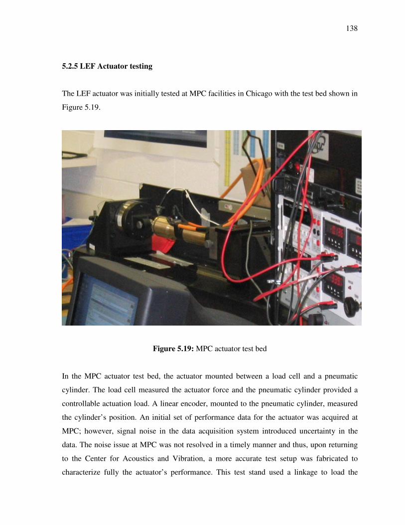
138
5.2.5 LEF Actuator testing
The LEF actuator was initially tested at MPC facilities in Chicago with the test bed shown in
Figure 5.19.
Figure 5.19: MPC actuator test bed
In the MPC actuator test bed, the actuator mounted between a load cell and a pneumatic
cylinder. The load cell measured the actuator force and the pneumatic cylinder provided a
controllable actuation load. A linear encoder, mounted to the pneumatic cylinder, measured
the cylinder’s position. An initial set of performance data for the actuator was acquired at
MPC; however, signal noise in the data acquisition system introduced uncertainty in the
data. The noise issue at MPC was not resolved in a timely manner and thus, upon returning
to the Center for Acoustics and Vibration, a more accurate test setup was fabricated to
characterize fully the actuator’s performance. This test stand used a linkage to load the

139
actuator and an optical encoder to measure the actuator speed. The linkage loaded the
actuator using a force-amplifying lever arm and a weighted bucket at the arm’s end. The
optical encoder timed the duration of a single rotation of the upper nut. Therefore, an
average linear actuation velocity over one rotation of the nuts was determined by taking the
ratio of the screw thread pitch (0.2 inch) and the encoder-measured time for a single
rotation. This measurement method gave repeatable and accurate performance data. The new
test setup is shown in Figure 5.20.
Figure 5.20: Feed-screw actuator test apparatus
The equivalent actuator load of the lever arm and empty bucket was 80 lbs. The lever arm
load amplification between the weighted bucket and the actuator was a factor of 17, and
therefore, five-pound increments at the bucket gave 85 lb load increments at the actuator.

140
Three timed actuation trials were measured and averaged at each constant bucket weight or
actuation load. The averaged speed and load data for the 100 Hz stack driving frequency and
-200 to 1000 Vpp bi-polar voltage (as limited by the power supply) are shown in Figure 5.21
a). The power versus speed performance was calculated using the measured load and speed
data to give Figure 5.21 b).
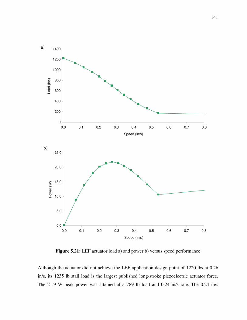
141
Figure 5.21: LEF actuator load a) and power b) versus speed performance
Although the actuator did not achieve the LEF application design point of 1220 lbs at 0.26
in/s, its 1235 lb stall load is the largest published long-stroke piezoelectric actuator force.
The 21.9 W peak power was attained at a 789 lb load and 0.24 in/s rate. The 0.24 in/s
0.0
5.0
10.0
15.0
20.0
25.0
0.0 0.1 0.2 0.3 0.4 0.5 0.6 0.7 0.8
Speed (in/s)
Pow
er (
W)
0
200
400
600
800
1000
1200
1400
0.0 0.1 0.2 0.3 0.4 0.5 0.6 0.7 0.8
Speed (in/s)
Load
(lb
s)a)
b)
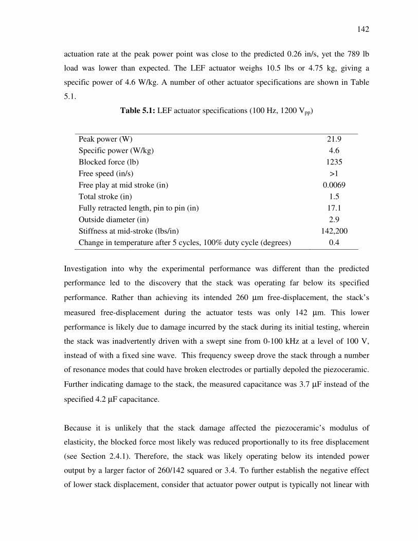
142
actuation rate at the peak power point was close to the predicted 0.26 in/s, yet the 789 lb
load was lower than expected. The LEF actuator weighs 10.5 lbs or 4.75 kg, giving a
specific power of 4.6 W/kg. A number of other actuator specifications are shown in Table
5.1.
Table 5.1: LEF actuator specifications (100 Hz, 1200 Vpp)
Peak power (W) 21.9 Specific power (W/kg) 4.6 Blocked force (lb) 1235 Free speed (in/s) >1 Free play at mid stroke (in) 0.0069 Total stroke (in) 1.5 Fully retracted length, pin to pin (in) 17.1 Outside diameter (in) 2.9 Stiffness at mid-stroke (lbs/in) 142,200 Change in temperature after 5 cycles, 100% duty cycle (degrees) 0.4
Investigation into why the experimental performance was different than the predicted
performance led to the discovery that the stack was operating far below its specified
performance. Rather than achieving its intended 260 µm free-displacement, the stack’s
measured free-displacement during the actuator tests was only 142 µm. This lower
performance is likely due to damage incurred by the stack during its initial testing, wherein
the stack was inadvertently driven with a swept sine from 0-100 kHz at a level of 100 V,
instead of with a fixed sine wave. This frequency sweep drove the stack through a number
of resonance modes that could have broken electrodes or partially depoled the piezoceramic.
Further indicating damage to the stack, the measured capacitance was 3.7 µF instead of the
specified 4.2 µF capacitance.
Because it is unlikely that the stack damage affected the piezoceramic’s modulus of
elasticity, the blocked force most likely was reduced proportionally to its free displacement
(see Section 2.4.1). Therefore, the stack was likely operating below its intended power
output by a larger factor of 260/142 squared or 3.4. To further establish the negative effect
of lower stack displacement, consider that actuator power output is typically not linear with

143
the stack’s power output. This is because actuator backlash negates a fixed amount of a
stack’s stroke. Therefore, if there were a 42 µm backlash, the equivalent difference between
the actuator’s performance with a new versus damaged stack would be a factor of 218/100
squared. In addition, contact stiffness between the nuts and their supporting surfaces can be
hypothesized to act as a nonlinear stiffening spring—according to Hertizian contact
theory—giving a similar affect as was described for backlash. Thus, if provided with a new
260 µm free-displacement stack, the actuator would likely exceed the LEF application’s
specified design point for first quadrant operation. Achieving second quadrant operation will
be addressed in Section 5.3.
Referring back to Figure 5.21 a), notice that at low loads the actuator’s force versus speed
curve does not follow the linear decline to zero—as is characteristic of most piezoelectric
actuators. Here, a unique trend exists because the actuator’s net performance is in fact the
superposition of the piezoelectric stack’s performance and that of the electromagnetic motor.
Therefore, at loads below 200 lbs, the electromagnetic bias motor output dominates the
actuator’s performance characteristics, and the actuator exhibits a unique high-speed output.
However, this actuation performance is not of interest here because it is the typical and
conventional electromagnetic feed-screw actuator behavior of an actuator powered by the
bias torque motor. Nonetheless, it follows that the free speed of the actuator is
approximately the product of the free speed of the electromagnetic motor and the screw
thread pitch. Therefore, the motor’s free speed of 1200 RPM and the 0.2 inch screw thread
pitch gives an actuator free speed of 4 in/s (this free speed is estimated because the optical
encoder setup could not measure speed at this high level).
In these initial feed-screw actuator tests, reliable direction reversal was only achieved at
loads below 250 lbs. This was due to the conservative design of the screw pitch angle and a
incorrect estimation of its surface friction coefficients. A simple experimental test using a
torque meter and a known load indicated that the Coulomb and static coefficients of friction
were 0.20 and 0.22 instead of the expected 0.08 and 0.15, respectively.
144
In addition to only reversing at low loads, the characteristics of the second quadrant
operation were undesirable. In reverse or second quadrant operation, the nuts would enter a
random stick-slip or chatter behavior. This was hypothesized to be caused by the difference
in the static and dynamic friction behavior of the nut and screw.
5.3 Improving the LEF feed-screw actuator
At this stage in the project, achieving second quadrant operation under higher loads was
paramount to the success of the feed-screw piezoelectric actuator project. To enable second
quadrant operation, there are a number of different methods to free the nut under the aiding
load: These including increasing the motor torque, increasing the wedge angle or screw
pitch angle, or decreasing the coefficient of friction of the surfaces. Reducing the nut-screw
surface coefficient of friction appeared to be the easiest method because it did not require
modification of the actuator. Various lubricants such as caster oil, aircraft grade greases
(Aero-shell, Brayocote, and Mobile 28), and graphite power on dried surfaces had little
effect on the contact surfaces’ coefficient of friction. This fact, in addition to the large
measure coefficient of friction, is likely related to the high contact pressure that may have
squeezed the lubricant film layer out of the screw-nut surface contact regions (~3 kpsi at the
base of the nuts under a 1000 lb. load).
5.3.1 Nut roller thrust bearings
The second method attempted for improving second quadrant operation involved inserting
roller thrust bearings between the nuts and their contact surfaces (the nut support plate for
the holding nut and the stack cap for the driving nut). In this way, the only significant
frictional locking contact is between the nut and screw threads. To provide a race for the
thrust bearings, adapter rings were fabricated and attached to the nuts. Spacers were also
inserted between the bottom cap and the housing, and the top cap and the nut support plate
to provide space for the new bearings.

145
Figure 5.22: Roller thrust bearing and race located between the holding nut and the nut support plate
These modifications significantly improved the second quadrant operation, while also
unexpectedly improving first quadrant actuation. The improvement in the first quadrant
performance was due to the added trust from the bias torque motor and a better seating
between the nut and its supporting surfaces. The following plot summarizes the new
performance of the actuator with the thrust bearings.

146
Figure 5.23: Load versus speed performance plots with thrust bearings
An impressive second quadrant actuation load of 900 lbs and a higher 28.8 W peak power
output was achieved. Another important advantage of using thrust roller thrust bearings is
that the nuts could conceivably be located between two thrust bearings in a preloaded
sandwich configuration, which could reduce the clamp compliance and eliminate backlash.
This configuration would be particularly valuable for four-quadrant control, wherein the
nuts are required to support bidirectional load.
Nevertheless, in this thrust bearing design, the problem of erratic downward motion
remained. This was primarily because of the stick-slip’s behavior and the poor control of the
electromagnetic motor. The controller was designed to perform basic control, and therefore
it either functioned in a torque control mode (wherein the current supplied to the motor coils
is proportional to an analogue input signal), or in a speed-controlled mode (where the
voltage is controlled). A better motor controller using nut position feedback could
significantly improve the second quadrant operation of the actuator. However, a simpler and
inherently more robust method for improving the characteristics of the second quadrant
operation was to use an ultrasonic piezoelectric bias motor.
0
200
400
600
800
1000
1200
1400
0.0 0.1 0.2 0.3 0.4 0.5 0.6 0.7 0.8
Speed (in/s)
Load
(lb
s)Original configuration
Nut thrust bearings

147
5.3.2 Ultrasonic bias motor
Ultrasonic traveling wave motors are ideal for controlling second quadrant operation
because the friction contact that drives the ultrasonic motor provides a simultaneous torque
and velocity control. In this way, overriding loads on the ultrasonic motor are passively
resisted if the rotor exceeds its intended velocity. An additional benefit of the ultrasonic
motor is that it acts as a brake in its off position. This is important in spite of the LEF
actuator’s self-locking capability because external high frequency vibration on the actuator
could induce drift of the electromagnetic motor and nuts, thereby inadvertently allowing the
actuator to move. In addition, an ultrasonic motor used for this application dose not require
encoder position feedback, thereby simplifying the actuator assembly.
The low speed and high torque of standard Shinsei ultrasonic motors matches well with the
~100 rpm speed required to operate the actuator at its 0.26 in/s intended rate. To develop the
2 N-m stall and 1 N-m continuous rated torque, two standard Shinsei motors were required.
Integrating the two Shinsei motors into the actuator involved disassembling them and
fabricating custom mounting hardware. The heavy ball bearings required in the
electromagnetic motor to maintain the radial and axial alignment of the rotor and stator were
not required for Shinsei ultrasonic motors. Instead, small nylon bushings were sufficient to
support the rotor. The Shinsei motor subassembly is approximately 1/3 the mass and takes
up 1/3 the volume of the electromagnetic motor subassembly, which in turn reduced the
actuator’s weight to 9.7 lbs. The new Shinsei motor subassembly is shown in Figure 5.24.

148
Figure 5.24: Shinsei ultrasonic bias torque motor assembly with torsion spring couplers
The new modified actuator design with the thrust bearings and the Shinsei motors is shown
in the Figure 5.25.
Figure 5.25: Computer model of feed-screw actuator with integrated thrust bearings and Shinsei motors
An important consideration for implementing the ultrasonic motors in the actuator housing
was the critical compressive preload that holds the rotor and stator together. The
compressive preload was applied to the motor by threading the nut support plate into the

149
actuator housing. Thin shims were experimentally added or removed to adjust the load until
the externally applied torque required to rotate the rotor was 2.0 N-m, which is the blocked
torque of the two Shinsei motors.
A drawback of using the ultrasonic motors was a slight decrease in bias torque. The lower-
than-intended torque is likely due to a number of factors involving integration of the motors
into the actuator housings. These factors include the following: a cracked segment of one of
the ultrasonic motor’s piezoceramic, poor alignment between the rotor and stator, and
changes in the stator resonance properties due to mounting modifications. The reduced
performance of the ultrasonic motor–based actuator (with thrust bearings) is shown in
Figure 5.26.
Figure 5.26: Load versus speed feed-screw actuator with thrust bearings and Shinsei motors
Comparing the ultrasonic-based actuator to the electromagnetic-based actuator, the stall
torque was reduced to 1140 lbs and the peak power was reduced from 28.8 W to 20.1 W.
The specific power of the new electromagnetic thrust bearing and ultrasonic motor
0
200
400
600
800
1000
1200
1400
0.0 0.1 0.2 0.3 0.4 0.5 0.6 0.7 0.8
Speed (in/s)
Load
(lb
s)
Original configuration
Nut thrust bearings
Ultrasonic motor and bearings

150
configurations are 6.1 and 4.8 W/kg, respectively. These performance specifications are
summarized in Table 5.2.
Table 5.2: Performance specification comparison
Original design Thrust bearing design Ultrasonic motor design Power (W) 21.9 28.8 20.1 Specific power (W/kg) 4.6 6.1 4.8 Blocked force (lb) 1235 1235 1140
In spite of the lower performance of the ultrasonic-based actuator, it was successful in that
both first and second quadrant operation were achieved and its second quadrant operation
was smooth and controlled. This was a substantial accomplishment in the feed-screw
actuator development effort and is of great significance to this dissertation.
5.3.3 Other experimental work
There were a few remaining experimental tests of interest—namely, determining the
influence of stack driving frequency, the relative nut positions, and the precision of the feed-
screw on the actuator’s performance. The relationship between the actuator’s power output
and the stack driving frequency was of prime interest, because increasing the drive
frequency is a simple method for improving the actuator speed. Due to limited frequency
range of the Qortek power supply, the actuator’s peak output was only measured at various
frequencies between 50 and 100 Hz.

151
0
5
10
15
20
25
40 50 60 70 80 90 100 110
Frequency (Hz)
Pow
er (
W)
Figure 5.27: LEF actuator power versus frequency relationship
Interestingly, the power output more than doubled between the 50 and 100 Hz driving
frequencies. Based on this trend and the initial model predictions, the power output is
expected to roll off gradually, peaking at a ~250 Hz drive frequency and ~40 W peak power.
The roll-off in the power is due to the dynamics of the nuts and bias motor, preventing them
from effectively accumulating the stack’s stroke at high frequencies.
The next experimental test of interest was determining how the relative nut position affects
the actuator’s performance. This test involved adjusting the driving nut’s rotational position
with respect to the holding nut and measuring the actuator’s performance. The performance
results are shown in Figure 5.28.

152
Figure 5.28: Influence of relative nut positions on power output
In Figure 5.28, the ‘0’ nut position refers to the original nut position used in all the prior
actuator tests. It corresponds to the position where both nuts contact their supporting
surfaces under a no load condition. The other numbered nut positions on the horizontal axis
correspond to advancement of the holding nut by 1,2,3 or -1,-2,-3,-4 factors times the 18
degree nut rotation that translates the nut a distance equal to the stack’s free displacement.
The optimum relative nut position was near zero. Both advancing and rotating the holding
nut backwards caused a significant decline in the power output of the actuator.
Another interesting topic that was addressed experimentally was determining the importance
and ultimately the influence of the screw and nuts’ precision tolerances on the actuator’s
performance. This was of interest because fabricating the LEF actuator’s precision screw
and nuts accounted for half of its net machining cost (the reasoning behind using the tight
tolerances was to ensure proper alignment and a low structural compliance in the nut and
screw interface). To determine the influence of the precision tolerances, MPC’s screw and
nuts were replaced with a standard ACME screw and bronze nuts. It was found that this
modification had little effect on the actuator’s performance as is shown in Figure 5.29.
0
5
10
15
20
25
-5 -4 -3 -2 -1 0 1 2 3 4 5
Nut Position
Pow
er (
W)

153
0
200
400
600
800
1000
1200
1400
0.0 0.1 0.2 0.3 0.4 0.5 0.6 0.7 0.8
Speed (in/s)
Load
(lb
s)
MPC screw and nuts
Bronze nuts and standard screw
Figure 5.29: Conventional screw compared to MPC’s precision screw
To test the actuator’s robustness, a 10 lb external side-load was applied to the actuator in an
effort to induce misalignment between the screw and nuts. Remarkably, the side load, shown
in Figure 5.30, did not affect the actuator’s performance, indicating that the actuator design
is insensitive to adverse loading conditions and that a conventional screw and nut could be
used in the actuator without significantly degrading its performance.

154
Figure 5.30: Side load added to actuator to determine robustness of actuator
5.4 A perspective on the LEF actuator
The LEF actuator was successful in terms of demonstrating reliable actuation, but its 6.1
W/kg peak specific power performance is seemingly unimpressive. To place the LEF
actuator’s specific power performance into perspective, it is useful to compare the LEF
actuator to an ultrasonic motor driven actuator and an electromagnetic driven actuator that
use the same basic feed-screw configuration as the LEF actuator.
Consider, first, driving the LEF actuator’s 789 lb peak power load with Shinsei ultrasonic
motors in a simple feed-screw configuration (no longer using the stack and motion
accumulation). This is a useful technology comparison because the specific power
performance of Shinsei motors ranks among the best piezoelectric devices (see Figure 3.28).
To implement such an actuator and attain the same peak power point as the LEF actuator, a
number of Shinsei motors would need to be coupled in parallel. The peak power point of
Shinsei ultrasonic motors is 0.49 N-m at 100 rpm, and therefore, a screw with a 5 threads
per inch pitch would meet the 0.26 in/s rated speed requirement. Because the ultrasonic
motor is inherently self-locking while off, a ball screw with a 90% efficiency could be used

155
(ball screw efficiency is defined as the ratio of a rotation mechanical power input and the
resulting translation power output, or vice versa). To meet the rated speed and force
requirements, a minimum of 7 ultrasonic motors would need to be coupled in parallel.
Compactly integrating seven ultrasonic motors into a housing similar to that of the LEF
actuator housing would weigh approximately 3 kg; hypothetically giving a net 10.7 W/kg
specific power, which is slightly higher than that of the LEF actuator.
Now, consider another configuration wherein an electromagnetic motor is used in a feed-
screw configuration; in particular, consider using the original electromagnetic bias torque
motor. This is feasible because the peak power output of the bias motor is 42 W. At first
glance, it would appear odd that the peak power output of the bias motor is greater than that
of the LEF piezoelectric feed-screw actuator. However, considering that the peak power
point of the bias motor occurs at 800 rpm and the rated speed of the LEF application is a
slow 0.26 in/s speed, it is reasonable to assert that the bias motor could power the LEF
application, if coupled to an adequate force or torque amplification transmission mechanism.
Therefore, consider coupling the electromagnetic bias motor to a transmission with a 10:1
gear reduction ratio and an estimated 90% efficiency. Assuming that the transmission
couples to a standard 5 thread per inch, 62% efficiency ACME feed-screw, the bias motor
could operate at its peak power point and produce the approximate rated load and speed of
LEF feed-screw actuator [42]. Note that a standard ACME feed-screw, rather than a higher
efficiency ball screw, is required to maintain a self-locking condition in this case. To
determine the specific power of such an actuator, an assumption for the weight of the
transmission must be made. An off-the-shelf 10:1 gear reduction transmission capable of
handling a 42 W power throughput would weigh approximately 0.5 kg and have a size
comparable to that of the bias motor. This would give an approximately 2.5 kg actuator
weight and 9.4 W/kg specific power.
Comparing these example actuators with the LEF actuator’s 6.1 W/kg specific power
indicates that the LEF actuator is not on par with other actuator technologies in terms of
specific power. However, considering the stack was working at approximately 1/3 of its

156
peak power output and the driving frequency was restricted to a low 100 Hz by the power
electronics, it is reasonable to assume that a factor of ~6.8 improvement in specific power
could be attained by replacing the stack and using a higher frequency power supply (factor
of ~2 improvement due to increased driving frequency and factor of ~3.4 improvement with
proper stack operation). In addition, the design has not been optimized for specific power;
such a study is presented next in Chapter 6.

Chapter 6
ACTUATOR MODELING AND DESIGN OPTIMIZATION
Thus far, the conceptualization and experimental development of the piezoelectric feed-
screw actuator has been discussed. This development involved intuitive design optimization
for maximizing the actuator’s performance. While such optimization is useful as a starting
point, it is an inefficient process due to the dynamic behavior of the actuator. For example,
increasing the size of the nuts could reduce their structural compliance and improve the
actuator’s force output, but the increase in nut size could also slow the motion accumulation
response of the nuts and decrease the actuator’s speed. Experimental investigation of such
relationships would require dozens of prototypes and vast amounts of testing.
However, by developing a mathematical actuator model, design modifications can be
simulated by numerical experiments instead of fabricating new hardware. Nonetheless,
considering that there are numerous independent design parameters that influence the
actuator’s specific power, arriving at the optimum actuator design by manually adjusting
model parameters is still a daunting task. This problem is not, however, uncommon, and it is
typically addressed using optimization strategies. Hence, this chapter presents the
mathematical modeling and design optimization of the feed-screw actuator for maximizing
its specific power performance.
6.1 A dynamic feed-screw actuator model
6.1.1 Developing the basic actuator model
Classical design optimization involves searching within a design space for the set of design
variables that maximizes or minimizes an objective function while satisfying a set of
constraints. For the feed-screw actuator, the optimization objective function is the actuator’s
specific power and the design variables include parameters such as the thread pitch, screw
diameter, stack size, etc. Interestingly, formulating a computationally efficient and accurate

158
actuator model to evaluate the specific power objective function presents a more significant
challenge than carrying out the optimization. This is primarily due to the complexity of the
actuator’s mechanical system and highly dynamic behavior. In particular, actuator
component flexibility and inertia play important roles in determining the actuator’s
performance. Therefore, the actuator’s behavior is not only time-dependent but is also
defined by the actuator’s structural continuum. Considering this, a complex system of partial
differential equations is required to precisely describe the actuator’s dynamic behavior.
Solving such a system of equations for the actuator can be a formidable task.
Such problems are common in mathematical vibration analysis; in most cases, systems are
simplified by approximating continuous (infinite number of degrees-of-freedom) elastic
components as discrete or finite lumped masses, viscous dampers, and linear springs. In this
way, complicated dynamic systems are described by ordinary differential equations.
Discretizing mechanical systems in this way can involve using finite element methods or
treating rigid body components as individual degrees-of-freedom. In general, increasing the
number of degrees-of-freedom will improve the model accuracy at the cost of increasing
computation difficulty. Nevertheless, selecting a suitable set of degrees-of-freedom that
includes the important features of a system, while also minimizing the model complexity,
involves engineering judgment and model experimentation. For the feed-screw actuator,
selecting the actuator model’s degrees-of-freedom involved a somewhat iterative process in
which computationally efficient models were developed, compared to experimental results,
and adjusted to better represent the actuator or to simplify the model. The final actuator
model configuration is shown in Figure 6.1.

159
Figure 6.1: Dynamic model of hybrid actuator
tFS ωsin−
Motor
Screw
Stack
kc
kn
kc kn
kh
ksc
ks
mr
mn
mn
ms
mds
mhs
mh
xr
xdn
xds
xhn
xhs
xh
xs
Driving nut
Holding nut
Housing
Fbias
PL
Fdµ
Fhµ
Load
Csc ch
cs

160
Notice that the actuator model in Figure 6.1 is only suited to drive a unidirectional
(downward oriented) load. This simplification was adopted because demonstrating first and
second quadrant operation is sufficient to prove four-quadrant operation, as was previously
explained in Section 4.2.3.
In the planar actuator model, a stiff spring, end mass, and external forcing function
approximate the stack as a simple single degree-of-freedom body. The stack stiffness was
given by the ratio of its blocked force and free displacement ( FBF δ/ ). Because the stack is
nearly uniform in density along its length, its end mass was estimated by the sum of one-
third its total mass and the stack cap mass. In this way, the spring-mass model of the stack
will replicate the low (0-4 kHz) frequency dynamic behavior of the stack actuator. The stack
was driven with a fixed periodic sinusoidal voltage, and thus its external driving force was
modeled as the product of a time-dependent sine function and the stack’s force amplitude.
The amplitude of the stack’s driving force was given as the product of its blocked force and
the ratio of its driving voltage and maximum operating voltage (Max
BS VV
FF = ).
The screw-nut hybrid clamps were modeled by planar wedge configurations. Taking the
screw pitch diameter as a reference plane, the wedge mass was given by the product of the
nut inertia and square of the screw pitch radius ( 2rI Nut ) and the wedge angle was simply
defined by the screw thread pitch angle (). Because the screw stiffness is significant
relative to the stack stiffness, the screw was modeled as a two degree-of-freedom body. The
screw stiffness was defined by its elastic modulus, pitch diameter, and length between the
nuts. Interestingly, the screw’s torsion stiffness proved to have a negligible affect on the
actuator’s performance. Similarly, the housing torsion stiffness had a negligible influence on
the actuator’s performance while its longitudinal stiffness was critical. Thus, the housing
was modeled as a single degree-of-freedom body with an end mass approximated by one-
third its net mass. The housing stiffness was defined by its elastic modulus, length, and
average cross-sectional area. A damping ratio of 0.005 was used for the stack and the
structural components.

161
Accurately modeling the electromagnetic and ultrasonic bias motors proved difficult
because both types of motors exhibit a strong decline in torque with increasing speed. The
decline in torque with increasing speed behavior was modeled with a constant bias force and
damper connecting a rotor mass to ground. The rotor mass was taken as the product of the
rotor’s moment of inertia and the square of the screw pitch diameter. Thus, the motor’s
planar reference was taken about the screw pitch diameter to maintaining consistency with
the nut-screw interface reference.
Note that neither electromagnetic nor ultrasonic motor’s torque versus speed behaviors
follow a linear relationship, as is modeled by the rotor mass, viscous damper, and constant
bias force. Nonetheless, the feed-screw actuator demands a small range of motor speeds and
thus, it is reasonable to select a damping such that the model motor matches the actual
motor’s stall torque and peak power points. Therefore, the constant bias force was given by
the ratio of the motor stall torque ( BiasT ) and the screw pitch radius ( r ); the motor damper
was defined by the ratio of the motor’s torque at peak power (Tpp) and the product of its
corresponding angular velocity ( ppΩ in rad/s) and squared pitch radius. This damping
parameter is given as
2r
TTc
pp
ppBiasm Ω
−= (6.1)
The remaining (and, arguably, the most significant) aspects of the model to be discussed are
the normal contact and friction interface in the hybrid clamp. Unfortunately, simple static-
Coulomb and linear surface stiffness models are inaccurate for modeling high-speed and
intermittent contact behavior in the feed-screw actuator. Therefore, more accurate surface
interface models were sought after by looking to research literature.
Beginning with Leonardo da Vinci’s first documentation of static and kinetic friction in
1519, there has been a large body of research on surface modeling [43]. The science of
surface contact (tribology) is extremely active; presently, 700 articles are published on this
topic each year. The primary focus of most of the literature is not the dynamics of the

162
surfaces but rather is concerned with wear and surface chemistry. Friction force between
contacting bodies is affected by a long list of factors which include lubrication, surface
roughness, thermal effects, and wear [44]. Therefore, it is difficult to find simple models of
surface interaction that could be included in a useful hybrid actuator model. At present there
are no comprehensive models that take into account all the characteristics of surfaces in
contact [43]. However, approximate models that capture the general contact phenomena
have been chosen for the actuator model. In addition, tangential (friction) and normal
(surface stiffness) surface dynamics are interrelated, but attempts to model both
simultaneously prove difficult [45-47]. Therefore, independent mathematical descriptions of
each surface interaction are pursued herein.
6.1.2 Modeling the screw-nut interface stiffness
It is well known that surfaces are rough on a microscopic level. When two surfaces come
into contact, their interface can be visualized by imagining “Switzerland” flipped on top of
“Austria.” The peaks on the surfaces contact each other and create complex micro-scaled
deformations [48]. These microscopic peaks are referred to as asperities. A large body of
contact mechanics-based research has involved modeling the interface of asperities [49].
The pioneering work of Greenwood and Williamson in 1966 has become the primary
building block for many surface contact models and is the standard method for generating
simple and useful surface stiffness relations [50]. Greenwood proposed that a rough surface
can be represented by a height probability distribution of average sized asperities, as shown
in Figure 6.2.

163
Figure 6.2: Asperity representation and height probability distribution
The probability distribution and Hertzian contact mechanics can then be employed to
develop a nonlinear surface stiffness relation. The assumptions that must be made for
Greenwood’s model are: 1) the asperities are spherical at their tips; 2) the strains are within
the elastic limits of the material; 3) the area of contact is frictionless; and 4) the contact
deformations are small compare to the asperity radius.
Greenwood’s model can be explained by beginning with defining a height probability
density across the contacting surface. The probability density function )(zφ describes the
probability with which an asperity at a height z above the reference plane exists. Gaussian,
exponential, and linear asperity distributions have been considered in the literature.
However, a simple rectangular distribution has agreed well with experimental surface profile
data [50]. The rectangular distribution is given by
Lz
1)( =φ , ( Lz <<0 ) (6.2)
The probability that a single asperity will be in contact at a surface separation distance of d
can be found by integrating the probability density function over the interference distance of
the surfaces and is given by
=L
ddzzdp )()( φ (6.3)
R )(zφ
z
z d
Reference plane Asperity height probability density function Rough surface
profile
Gaussian distribution
Constant distribution

164
Using Hertzian contact theory, the contact force for a single spherical asperity can be written
as
2/32/1 )(34
)( dzERzP −= (6.4)
The parameter E is the material elastic modulus and R is the mean radius of the asperity
peaks. Combining Equation 6.3 and 6.4, the net contact force can be written as
=L
ddzzPzNdF )()()( φ (6.5)
Defining a surface interference distance as dL −=δ gives the simple force-displacement
relation
2/52/1
158
)( δδ ERLN
F = (6.6)
Inspection of Equation 6.5 yields the important idea that surface stiffness may not dependent
upon the area of the contacting surfaces. This is the case if N/L and R are independent of the
contact surface area. R is clearly independent of the contact area and is only dependent on
the surface roughness. The ratio N/L can also be assumed to be independent of the contact
area because both N and L will likely be directly proportional to the contact surface area.
This is reasonable because N (the number of asperities) is proportional to the size of the
surface contacts. Considering that the surface machining tolerance is directly governed by
the height L of the asperity probability distribution, the machining tolerance is proportion to
area, as should L.
Assuming that surface stiffness is not dependent on the size of the surfaces is important to
the actuator model because a standard surface stiffness relation can be used for any scale of

165
actuator. It is also important because in this case the parameters N, L, R, and E may be
lumped into one parameter to give
2/5)( δδ csn CF = (6.7)
Nonlinear contact stiffness introduces significant complexity in solving the actuator’s
dynamic system of governing equations. However, this nonlinear surface interface behavior
only plays an important role during two critical loading scenarios: at the peak or maximum
nut-screw load and the load at which the bias torque begins to rotate the nuts. Accurately
modeling the screw-nut interface at the maximum load is important because it dictates the
peak reduction in the stack’s actuation stroke due to deformations in the nut-screw, -
housing, and -stack cap interface. The second important surface contact scenario occurs at
the point when the bias torque begins to rotate the nuts and accumulate the stack’s stroke.
Thus, modeling the contact surface stiffness with a single linear stiffness could lead to
improper nut accumulation behavior or inaccuracies in the actuator’s performance.
To circumvent the complexity of implementing nonlinear contact stiffness in the actuator
model while minimizing the error resulting from a linear stiffness approximation, a two-
linear stiffness model was adopted for the actuator model. The two-stiffness approximation
was implemented such that the model matched the displacement and force at each of the two
critical scenarios as shown in Figure 6.3.

166
Figure 6.3: Two-stiffness approximation model
Following a similar static hybrid clamp force analysis as given in Section 4.2.3, K1 and K2
can be computed as
( )221
sin
cos
C
BiasFFµα
α+
= (6.8)
( ) ( )
5/3
22
52
521
1
1
11
sin
cos
+===
C
Biascs
cs
FCCF
FFK
µα
αδ
(6.9)
( )( ) 52
2252
2252
1
12
sincos
sincos
+−
+−=
−−
=CBiasL
CBiasLcs
L
L
FP
FPC
FPK
µαα
µααδδ
(6.10)
Because the governing stiffness parameter Ccs depends on factors such as surface flatness,
roughness, and alignment, it is difficult to analytically compute or even estimate.
Determining Ccs experimentally would also be difficult because the actuator hardware would
need to be heavily loaded and instrumented to measure displacements on a micron scale.
Instead, Ccs was found by matching the model to experimental data. Thus, the magnitude of
K1
K2
δ
nF
1F
LP
2/5)( δδ csn CF =

167
Ccs used in the model is not based on theoretical or empirical results. Rather, it is a sort of
adjustment factor that reconciles the model and experimental results. Care was taken in
selecting Ccs because, if it compensates for model inaccuracies, misleading actuator
modeling results may be found.
6.1.3 An accurate and computationally efficient friction model
Unlike normal surface contact, friction depends upon the dynamic interaction of the
contacting surfaces. In the case of flat, metallic, and smooth surfaces (characteristic of the
nut and screw), the friction forces involve two fundamental behaviors: 1) pre-sliding
stiffness and 2) velocity dependent fluctuation. These two phenomena can be explained by
referring again to the idea that surfaces have microscopic roughness or asperities. When
considering friction, the asperities can be thought of as elastic bristles, as shown in Figure
6.4.
Figure 6.4: Elastic bristle (asperity) model for sliding of surfaces
With regard to the bristle model, pre-sliding stiffness—also known as micro-slip—is caused
by spring-like deformation of the bristles ( χ ) before sliding occurs. For typical steel
surfaces, pre-sliding can be on an order of 5 m, thus making it a significant concern in
modeling the actuator [43]. Dahl first proposed a mathematical model to account for pre-
sliding behavior in 1952 [51]. The Dahl model has been widely used in the research
literature. In its most basic form, the Dahl model is given by
χ x

168
−=
CFF
ddF
1σχ
(6.11)
The σ parameter represents the stiffness of the bristles and CF is a steady-state Coulomb
friction force. The parameter χ represents the energy stored by the deflection of the bristles;
when the sliding direction is reversed, that energy is returned to the system. Equation 6.11
dictates a rising friction force with increasing displacement that saturates at FC. This friction
behavior is illustrated in Figure 6.5.
Figure 6.5: Example Dahl friction behavior
The basic Dahl model does not account for the important observation that friction force is
typically higher under a static condition than during sliding. This change in friction force
can be accommodated by the Dahl model by way of the Stribeck effect [52]. The Stribeck
effect characterizes a decrease in friction force with velocity. This effect is commonly
modeled by the discontinuous the static and kinetic friction forces. In practice, however,
there is a gradual decline in friction force with velocity as is illustrated in Figure 6.6.
Displacement
Friction force
FC

169
Figure 6.6: Stribeck velocity dependence of friction force
For lubricated surfaces, the Stribeck effect is thought to be related to the development of a
fluid boundary layer between the surfaces, while for dry surfaces it is thought to be related
to normal micro-oscillation of the bristles sliding past one another. The Stribeck effect can
mathematically be described by an exponential decrease in friction with increasing sliding
velocity, which is written as
( )2/)( SxxC eFFxg
−
∆+= (6.12)
The variable ∆F is the difference between the static and kinetic or Coulomb friction
coefficients and Sx is the Stribeck velocity that characterizes how rapidly the friction force
declines with increasing velocity.
Recently, Canudas incorporated the Stribeck effect into the Dahl model by setting CF in
Equation 6.11 equal to the rate dependent function )(xg . The Stribeck/Dahl model can then
be written in a more convenient form by multiplying both sides by velocity, giving
−=
)(1
xgF
ddF
σ
χ (6.13)
Friction force
Relative tangential velocity
FC
FS

170
An example variation of friction force versus time described by Equation 6.13 is shown in
Figure 6.7.
Figure 6.7: General behavior of friction with constant velocity and starting from rest
The parameters that characterize the bristle stiffness and the Stribeck effect are dependent on
the specific geometry and finish of the modeled surfaces; thus, they are typically determined
experimentally. Conducting such an experiment for the actuator nut-screw contact would
require a precision test stand and sophisticated data acquisition system. Coincidently, a
recent paper by Gaul used a slight variation on the Dahl-Stribeck friction model for an
application with a nearly identical surface contact and geometric configuration as the nut
and screw interface. In the paper, the mechanical resistance in a semi-active cylindrical pin
joint was tailored to control the damping properties of the joint. The pin joint used a hollow
cylindrical piezoelectric stack aligned with the joints pivot axis to apply a compressive load
to friction surfaces. Gaul’s model defined the friction coefficient as
( )x
e
xx
SxxC
2/010 2 σχµµ
σσχσµ +
+−+=
−∆
(6.14)
Gaul’s semi-active cylindrical joint had smooth lubricated steel surfaces that were
approximately the same size as the nut-screw interface. Thus, the same six friction
parameters that were experimentally determined by Gaul for his semi-active joint were
Friction force
Time
FC
FS

171
directly applicable to the nut-screw friction model. These six friction parameters are listed in
Table 6.1.
Table 6.1: Parameters for Gaul’s semi-active joint friction model
Dynamic coefficient of friction c 0.20
Difference between static and dynamic coefficients of friction 0.02
Bristle stiffness (m) 0 5.0x10⁻⁴
Bristle damping (s/m) 1 1.0
Viscous damping (s/m) 2 0.01
Stribeck velocity (m/s) sx 10-6
Using the Gaul model, the friction force is given as the product of the normal force given by
Equation 6.7 and the friction coefficient given by Equation 6.14 ( NFF µµ = ). Therefore, the
nut-screw friction force depends both on the nonlinear contact interaction of the surfaces and
the friction coefficient model.
6.2 Formulating and solving the model’s governing equations
Describing pre-sliding stiffness and rate-dependent friction phenomena is a significant
feature of the Dahl-Stribeck friction model, but its high degree of computational efficiency
is arguably its most important quality. The model’s computational efficiency and accuracy,
compared to a conventional static-Coulomb model, result from the fact that zero-velocity
friction transition times do not need to be computed. This is significant because the
discontinuous characteristics of the more typical static-Coulomb friction model can
introduce unrealistic behavior and slow computation.
While the Dahl-Stribeck friction model conveniently circumvents the static-Coulomb model
discontinuity, the two-stiffness approximation model introduces unavoidable discontinuities
in the actuator model. The screw-nut contact discontinuity occurs if the bias motor’s nut
advancement lags behind the advancement of the stack. In such instances, the nut threads

172
separate from the screw threads and the model’s nut-screw interface contact stiffness must
be set to zero. Although this behavior causes the model to differ depending on the interface
of the nuts and screw, the model remains linear away from the transitions. Thus, the actuator
model constitutes a piecewise linear system.
For the piecewise linear actuator system, a closed form analytic solution method was
preferred because of its computational efficiency and insightful dynamic results. However,
finding the periodic solution that satisfies the actuator piecewise linear behavior is difficult,
considering that any number of discontinuous transitions can occur during a single period.
For example, when the screw contacts the nut at a high frequency, the interaction is
effectively an impact, which can result in a bouncing nut-screw contact behavior, giving rise
to numerous transitions during a single stack driving period (the stack-nut interface is flat
and smooth and has a low damping). Further complicating the model solution, the number
and order of driving and holding nut transitions is not fixed, but varies with the driving
frequency, load, and system parameters. While these transitions in the actuator model would
cause difficulty in finding a closed form analytical solution, solving for the system’s
response can readily be accomplished using numerical methods.
Numerical integration methods generally involve sequentially stepping through time and
solving the model’s system of governing equations at discrete time increments. Over each
time step, a suitable variation of the displacement, velocity, and acceleration are assumed.
Numerical integration can easily accommodate discontinuous system changes by checking
the status of the nut-screw interface at each time step. Based on the status of the interfaces,
changes to the system can be made and the integration can continue.
6.2.1 Simulink actuator model
While there are many different tools and methods for implementing numerical time
integration, MATLAB Simulink was chosen to simulate the actuator’s behavior. Simulink is
an interactive graphical environment for simulating dynamic systems. The Simulink

173
platform can access most of MATLAB’s tools for algorithm development, data
visualization, data analysis, and numerical computation.
In Simulink, mathematical expressions are represented by series of block functions and
interconnecting flow arrows—in a similar fashion as the configuration of control block
diagrams. The Simulink blocks include functions such as summation, multiplications, and
integration. Thus, the set of dynamic equations defining the actuator’s behavior are input to
Simulink in the form of a block diagram. Developing the actuator’s set of governing
ordinary differential equations for the Simulink model was a routine vibration problem. The
actuator’s set of differential equations was initially derived using basic Newtonian free-
body-diagrams and then verified using Lagranges equation.
The actuator has seven important motion-based degrees-of-freedom, giving a set of seven
second order ordinary differential equations. Gaul’s friction model for the nut-screw
interface is governed by a first order ordinary differential equation, giving an additional two
friction-based degrees-of-freedom. Thus, the Simulink model was formulated with a top-
level block structure with seven equation of motion blocks, two friction model blocks, two
contact stiffness blocks (for implementing the two stiffness approximation model), and an
input and output block. An image of the actual Simulink model is shown in Figure 6.8.

174
Figure 6.8: Simulink model of actuator
Simulink can accommodate a layered structure of block diagrams where each block contains
a system of sub-blocks. Thus, the blocks shown in Figure 6.8 are analogous to subroutines in
a computer program.
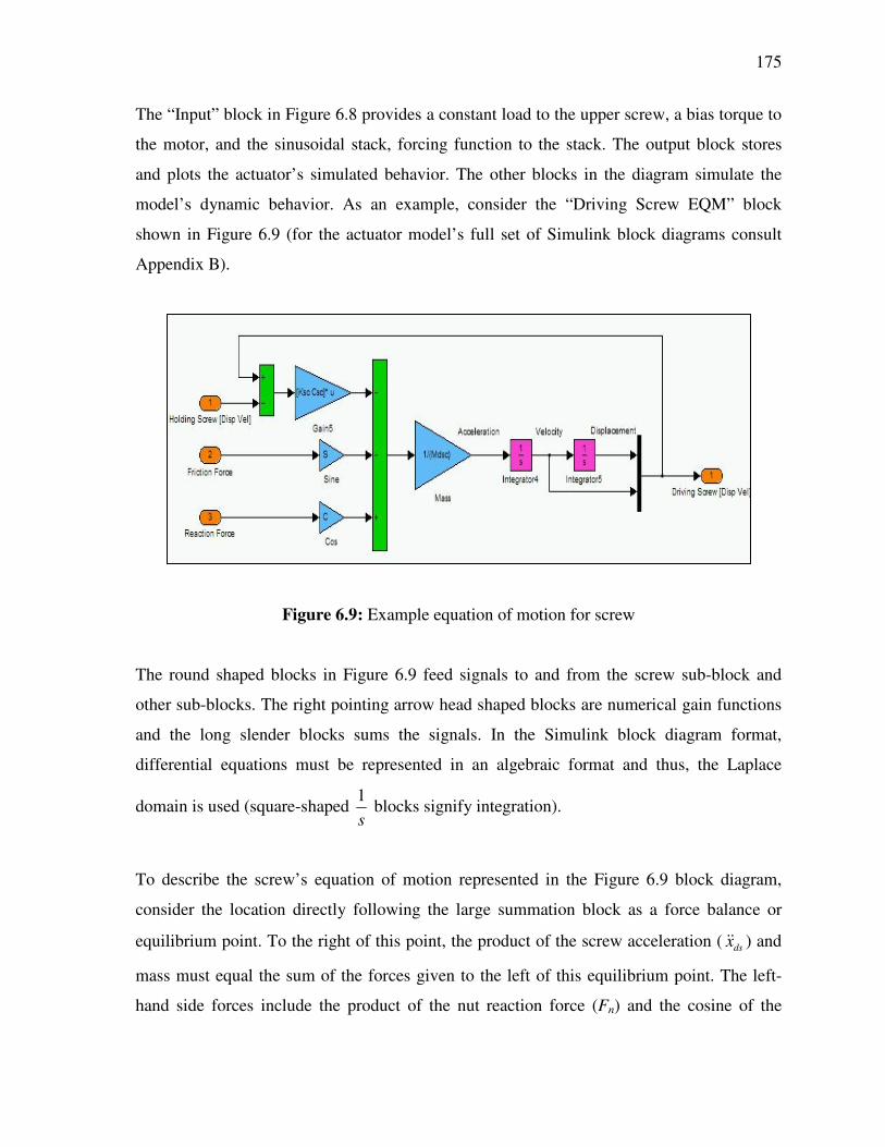
175
The “Input” block in Figure 6.8 provides a constant load to the upper screw, a bias torque to
the motor, and the sinusoidal stack, forcing function to the stack. The output block stores
and plots the actuator’s simulated behavior. The other blocks in the diagram simulate the
model’s dynamic behavior. As an example, consider the “Driving Screw EQM” block
shown in Figure 6.9 (for the actuator model’s full set of Simulink block diagrams consult
Appendix B).
Figure 6.9: Example equation of motion for screw
The round shaped blocks in Figure 6.9 feed signals to and from the screw sub-block and
other sub-blocks. The right pointing arrow head shaped blocks are numerical gain functions
and the long slender blocks sums the signals. In the Simulink block diagram format,
differential equations must be represented in an algebraic format and thus, the Laplace
domain is used (square-shaped s1
blocks signify integration).
To describe the screw’s equation of motion represented in the Figure 6.9 block diagram,
consider the location directly following the large summation block as a force balance or
equilibrium point. To the right of this point, the product of the screw acceleration ( dsx ) and
mass must equal the sum of the forces given to the left of this equilibrium point. The left-
hand side forces include the product of the nut reaction force (Fn) and the cosine of the

176
wedge angle (), the product of the friction screw-nut friction force (Fµ) and the sine of the
wedge angle, and reaction forces exerted on the screw from the holding section of the screw
(ksc and csc are the stiffness and damping of the screw section between the nut). This
equation of motion is written as
( ) ( ) 0cossin =−+−+−+ ααµ nhsdsschsdsscdssc FFxxkxxcxm (6.15)
6.2.2 Numerical simulation
The actuator model can be simulated using a number of different integration methods, but
some methods are more efficient and accurate than others for this problem. Simulink’s
ode45 variable-step method is the most appropriate numerical solver for this piecewise
linear actuator model [53]. The Simulink ode45 function is based on an explicit Runge-
Kutta formula. In the Runge-Kutta integration formulation, the current displacement is
expressed in terms of the immediately preceding displacements, velocities, and
accelerations. Using the new estimated displacement, the solution to the system of equations
is computed.
The accuracy of the simulation and the rate at which the actuator model converges to a
periodic solution dependents on the model’s behavior in the region of discontinuities or
transitions of the system. If the precise time at which a discontinuity occurs is not met by the
simulation, false conclusions about the behavior of the system may be observed. Consider,
for example, simulation of a bouncing ball. If the point at which the ball hits the floor occurs
between simulation steps, the simulated ball would appear to reverse position in midair. To
avoid this problem the time steps in the simulation must correspond with the instant at which
the system transition is occurring. Moreover, small time steps near the transitions are
required to accurately simulate the rapidly changing behavior of the system.
Simulink’s variable-step ode45 solver adjusts the step size dynamically, increasing the step
size when a variable is changing slowly and decreasing the step size when the variable

177
changes rapidly. Around a discontinuity, a variable changes extremely rapidly. Thus, in
theory, a variable-step solver should be able to hit a discontinuity precisely. The problem is
that to locate a discontinuity accurately, a variable-step solver must take exceedingly small
steps, slowing the simulation significantly.
Hence, to simulate discontinuities accurately without resorting to excessively small step
sizes, Simulink uses a technique known as zero-crossing detection. Zero-crossing detection
involves checking for discontinuities in the system’s state variables at each time step; if a
discontinuity is detected within the current time step, the precise time at which the
discontinuity occurs is determined. When a zero crossing is detected, Simulink interpolates
between the previous and current values of each variable that changed sign to estimate the
times of the zero crossings (e.g., discontinuities). Simulink then steps up to and over each
zero crossing. In this way, Simulink avoids simulating exactly at the discontinuity, where
the value of the state variable might be undefined.
In the actuator’s numerical simulation, its force-versus-speed performance was found by
determining its speed over a discrete range of constant loads. Hence, loads spanning the
actuator’s blocked force were incrementally applied to the model and the corresponding
actuation speed at each load was extracted from the simulation results.
The nut-screw interface stiffness constant was adjusted such that the model simulation
results match the experimental performance results. This stiffness parameter is given by
Ccs = 1.0x10¹² kN/m5/2. After adjusting the nut-screw interface constant, the Figure 6.10
simulated-versus-experimental LEF ultrasonic-based actuator performance results were
acquired.

178
Figure 6.10: Simulation and experimental force a) and power b) versus speed plots
The simulation fit well with the experimental performance over low speeds, but at high
speeds the simulation fidelity was poor because the ultrasonic bias motors began to
dominate the actuators performance characteristics. The performance of the ultrasonic motor
was approximated by a mass-damper model and thus, in accuracies at high speeds was
inevitable. However, in determining an actuator configuration’s specific power, the most
important performance point is the actuator’s peak power point, and at this location, the
0
5
10
15
20
25
0.0 0.1 0.2 0.3 0.4 0.5 0.6 0.7
Speed (in/s)
Pow
er (
W)
0
200
400
600
800
1000
1200
1400
0.0 0.1 0.2 0.3 0.4 0.5 0.6 0.7
Speed (in/s)
Load
(lb
s)Experimental data
Model simulation
a)
b)

179
simulation accurately correlated with the experimental results. To generate the simulation
curves in Figure 6.10, it took on average approximately 5 stack driving periods before the
actuator converged to a periodic solution (depending on the load and stack driving
frequency). Convergence was achieved over a broad frequency and load range that spanned
the stack’s first resonance frequency and the actuator’s blocked force. An example time
trace showing this convergence is for the driving nut and screw under an 800 lb actuation
load and a 100 Hz frequency is plotted in Figure 6.11.
Figure 6.11: Simulated time trace of screw and nut displacement
at actuator peak power point
The nut trace in Figure 6.11 is taken as the product of the nut rotation, the pitch radius, and
the tangent of the pitch angle. These two curves correspond to the nut-screw interface at a
fixed point on the screw threads, thus showing the screw stepping motion and the
advancement of the nut. Notice that for each driving period the screw is back-driven a
significant amount. This back-driving behavior is related to the undesirable structural
compliance in the actuator. Also, note that the nut closely tracks the motion of the
advancement of the screw, which reinforces the proposition in Chapter 5: that the 100 Hz
driving frequency is well below the point at which the nut dynamics limits the actuator’s
performance.
As a side note, the time required to simulate the actuator’s behavior over one complete stack
actuation period was on average 3 ms (for a 2 GHz processor). Thus, acquiring an average

180
actuation speed over 15 driving periods took about 0.5 s and the plots in Figure 6.10 with 20
performance points took approximately 10 s to generate.
6.3 Feed-screw actuator design optimization
6.3.1 Design variables and optimization approach
Having developed an accurate and computationally efficient model for simulating the
actuator’s performance, the next step was to vary actuator parameters or design variables in
an effort to find the optimum actuator design. Many different parameters define the actuator,
but only a handful are independent. For example, the nut diameter is related to the screw
diameter and the housing length is related to the stack and bias torque motor lengths.
Moreover, some design variables, such as the thickness of the bottom cap, have little effect
on the actuator’s performance, and can be neglected. Thus, by experimenting with the model
and using engineering intuition, the following design variables were found to be most
important for defining the actuator specific power performance: number of ultrasonic
motors, stack driving frequency, stack stroke, stack force, screw diameter, housing
thickness, screw pitch angle, and motor-nut coupler stiffness. In the case of an
electromagnetic bias motor, the design variables differ in that the bias motor is defined by its
rotor length and diameter.
Consider changing each parameter independently about the current LEF actuator
configuration to find the optimum actuator design that maximizes its specific power. This
sort of parametric survey gives the following power trends in Figure 6.12.

181
Figure 6.12: Parameter study plots
Note that the power output in Figure 12 is much higher than that simulated in Figure 6.10 b).
This is because the stack was taken to be operating at its full 260 µm free-displacement. The
horizontal axis in each plot is the ratio of the new design variables to the current ones (1.0 is
the original design configuration). Because they show only an orthogonal sampling of the
actuator’s design space about the original configuration, the trends in Figure 6.12 provide
little insight about how to improve the actuator. Such plots represent a very small survey of
the total design space. Thus, to use the model for a meaningfully optimization, combinations
of the design variables must be evaluated. Therefore, consider using ten data points per
design variable to evaluate the actuator performance (30 were used in Figure 6.12), 109
model simulations would be required to fully characterize the actuator’s design space. At
~0.5 sec per evaluation (for a 2 GHz Pentium 4 processor), it would take 322 yrs to optimize
the actuator’s design. Clearly, a more efficient method than sampling the entire actuator’s
design space is required to determine the optimum actuator design.
0
10
20
30
40
50
60
70
0.0 1.0 2.0 3.0 4.0Screw pitch angle
Pow
er (W
)
b) a)
0
10
20
30
40
50
60
70
0.0 1.0 2.0 3.0 4.0
Ultrasonic motor torque
Pow
er (W
)
Ultrasonic motor ratio Screw pitch angle ratio

182
6.3.2 A direct search optimization method: Simulated annealing
Optimization problems of this nature have spurred the growth of an entire area of applied
mathematics—primarily over the last 50 years—and there are standard techniques and
algorithms for dealing with such optimization problems. Nonetheless, the actuator
optimization problem is somewhat unique in that the specific power objective function is
discontinuous at points where the frictional locking condition is not met and the actuator’s
performance instantaneously falls to zero. Thus, some of the more common gradient-based
method’s optimization techniques are not fit for the actuator optimization problem
(MATLAB standard optimization functions use gradient-based “sequential quadratic
programming” methods) [54]. Instead, a direct search or zero-order method, requiring only
function evaluations, is most suitable for the actuator optimization. Further complicating the
optimization problem, the specific power objective function has local minima (maxima).
The two most prevalent direct search optimization methods for dealing with local minima
problems are “simulated annealing” and “genetic algorithms.” These direct search methods
are more computationally demanding than gradient-based methods, but are robust and are
adept at finding the global minima [55].
Further preferential selection of the optimization method could not be made at this point;
thus, the simulated annealing method was selected for performing the actuator’s design
optimization. The simulated annealing method takes its name from the process of annealing
or relieving residual stress in a material. Typically, residual stress or hardening of a material
is accomplished by quickly cooling the material such that some of its atoms become trapped
in high energy states. Annealing involves slowly cooling a material such that the high-
temperature random motion of the atoms allows them to adjust to a stable lower energy
states. During this cooling process, the probability of an atom moving to higher energy state
decreases with the decreasing temperature. Thus, during the annealing process, the energy at
a given location in the material will occasionally increase in accord with a probability
function. In this way, the net energy of the material can move out of local minima to arrive
at the global minimum.

183
The simulated annealing algorithm has parallels to material annealing in that the objective
function is analogous to the material’s energy and the design variables are analogous to
atoms. A typical simulated annealing algorithm consists of the four embedded loops shown
in Figure 6.13.
Figure 6.13: Simulated annealing algorithm
Design variable loop
Randomly increment a design variable
Evaluate the objective function f (call Simulink model)
If specific power is greater than the reference, accept the new design as the reference
If it is less than reference, accept it according to a temperature-dependent probability function
Cycle loop
Step adjustment loop
Adjust step size so that ~1/2 of the new designs are accepted
Reduce temperature to narrow probability of accepting a design with a specific power lower than the reference
Update the stored maximum specific power and optimum design
Compare new optimum specific power to the previous temperature iterations and exit routine if within a specified tolerance
Temperature loop

184
The inner design variable loop involves randomly stepping each design variable
(individually), evaluating the objective function, and accepting or rejecting the new actuator
design based on a specific set of conditions. Next, a cycle loop repeats the inner design
variable loop to broaden the optimization search. For each set of design cycles, the step
adjustment loop changes the randomly generated design variable step sizes to improve the
optimization search. Finally, to force the design search to converge upon the optimum
actuator, the outer temperature loop reduces the probability of accepting new actuator
designs.
In the design variable loop, accepting an actuator design involves setting a previously
accepted or reference set of design variables equal to the newly evaluated design variables
(xref = x). A new actuator design is always accepted if its specific power (objective function
evaluation) is greater than that of the reference design (f > fref). However, to prevent the
optimization search from prematurely converging to a local optimum design, about half of
the lower specific power designs are accepted according to a probability function given by
Tff ref
ep−
= (6.16)
Thus, if p is greater than a randomly generated number r (between 0 and 1), the design is
accepted and the lower specific power design is set as the reference design. This condition is
referred to as the Metropolis criterion [55]. The variable T in Equation 6.16 is analogous to
the temperature of an annealing material and it controls the probability of accepting lower
specific power designs. As the optimization search is carried out, the variable T is reduced
by a constant factor for each outer temperature loop. In this way, the optimization narrows
its search scope as it progresses.
This optimization search is most efficient if there are approximately the same number of
design rejections and acceptances. To maintain this balance, the design variable’s step sizes
are adjusted at the end of each step adjustment loop. Stepping the design variables involves
taking the difference between a current design variable refix and the product of a randomly
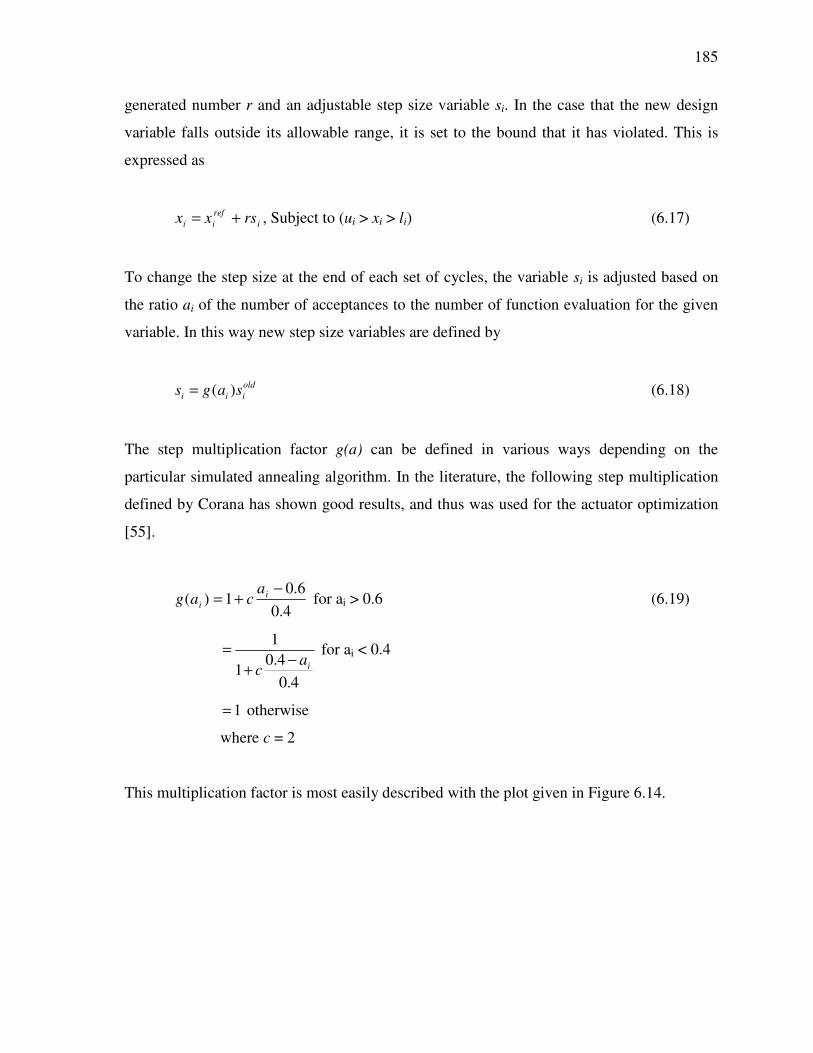
185
generated number r and an adjustable step size variable si. In the case that the new design
variable falls outside its allowable range, it is set to the bound that it has violated. This is
expressed as
irefii rsxx += , Subject to (ui > xi > li) (6.17)
To change the step size at the end of each set of cycles, the variable si is adjusted based on
the ratio ai of the number of acceptances to the number of function evaluation for the given
variable. In this way new step size variables are defined by
oldiii sags )(= (6.18)
The step multiplication factor g(a) can be defined in various ways depending on the
particular simulated annealing algorithm. In the literature, the following step multiplication
defined by Corana has shown good results, and thus was used for the actuator optimization
[55].
4.06.0
1)(−
+= ii
acag for ai > 0.6 (6.19)
4.04.0
1
1
iac
−+= for ai < 0.4
1= otherwise
where c = 2
This multiplication factor is most easily described with the plot given in Figure 6.14.

186
Figure 6.14: Step multiplication factor versus acceptance ratio
At the end of each temperature iteration, the global maximum specific power (fmax) and
corresponding design (xopt) is updated. The optimization continues indefinitely until fmax
repetitively falls within a specified tolerance, at which point the search routine is interrupted
and the optimization is complete.
6.3.3 Optimal LEF actuator design
Having developed and assembled a computationally efficient model and coupled it to an
appropriate optimization algorithm, we addressed the actuator design optimization problem.
As a starting point, the optimum actuator design for the LEF application was determined.
For the LEF application a rated load and speed were specified, and thus, specific power
optimization involved minimizing the weight of the actuator while achieving the rated
actuation requirements. However, the actuation rate depends on the actuator load and it is
not a specifiable design variable. To address this issue, the external actuation load was fixed
at the LEF rated load and designs with speeds differing more than +10% and -0% from the
rated speed were penalized by taking the product of the design’s specific power and the
percent difference between the design’s speed and rated speed.

187
In conducting the LEF actuator design optimization, the set of eight design variables
included: the number of ultrasonic motors, stack driving frequency, stack stroke, stack force,
screw diameter, housing thickness, screw pitch angle, and motor-nut coupler stiffness
(respectively given as ),,,,,,,( khtsbfreqnu qqqqqqqqf αφδ ). Rather than using the actual
numerical actuator values for the design variables, generalized actuator parameter
multiplication factors, pertaining to the original LEF actuator design, were used for the
design variables. For example, a stack length design variable of 1.0 corresponded to the LEF
actuator stack’s length and 2.0 was double that of the LEF actuator. Hence, each design
variable represents a change about the original actuator design.
To enhance the efficiency of the optimization search, the feasible design space was
selectively narrowed by tailoring the bounds for each design variables. In particular, a
maximum frequency limit was defined as 80% of the frequency corresponding to the
fundamental mode of the spring-mass stack model. Minimum bounds for the screw diameter
and housing diameter were chosen using the specified load and a safety factor of 5 (this
large safety factor was chosen because dynamic loading can be considerably larger than the
static load). Other bounds were selected to encompass a broad range of designs.
An additional constraint was defined to control the stack’s aspect ratio (the stack length to
diameter ratio): If the stack is too slender, buckling could occur. Based on the range of stack
aspect ratios that are commercially produced, a 2.0 aspect ratio limit with respect to the
original LEF stack was defined.
The LEF actuator’s success with ultrasonic bias motors prompted the LEF actuator
optimization to focus on using ultrasonic motors rather than an electromagnetic one.
Compared with electromagnetic motor data, there is not a wealth of experimental ultrasonic
motor performance data to confidently base an empirical relationship between motor
performance and size. Therefore, in the LEF optimization, the defining bias motor design
variable was the number of ultrasonic motors that would be coupled in parallel. In the
original LEF actuator, two ultrasonic bias motors were used; thus, the feasible range of the

188
number of ultrasonic motors variable was 0.5, 1.0, 1.5 etc (0.5 corresponds to a single
Shinsei ultrasonic motor). The aspect ratio and variable bound constraints were implemented
in the simulated annealing design variable loop.
To compute the actuator’s specific power, a relationship between the design variables and
the actuator mass was required. Considering the distribution of mass between the housing,
screw, stack, and bias motor and the influence of the design variables on each component’s
mass, the actuator mass was given as
( )( nuhtnet qqqm 3.07.00.1 += δ Housing
( )nus qqq 5.05.00.1 2 ++ δφ Screw
Bqqδ0.1+ Stack
)nuq5.0+ Bias torque motor
3.1× Misc. hardware (6.20)
To match the LEF actuator’s mass distribution, a 1.3 multiplication factor was added to the
actuator mass expression to account for miscellaneous hardware such as fasteners and the
spherical actuator mounting joints.
The actuator specific power was given by the ratio of the Simulink power performance and
the actuator mass (kg) from Equation 6.20. Because Simulink works seamlessly with
MATLAB, the optimization routine was written as a MATLAB program (see Appendix C
for simulated annealing code). In the optimization routine, the Simulink actuator model was
called to evaluate the actuator’s specific power for each set of design variables.
The simulated annealing algorithm converged to the optimum LEF actuator design after
5301 objective function evaluations. The optimum design is described in Table 6.2.

189
Table 6.2: Optimum LEF actuator design
Design Variable Multiplication Factor
Number of ultrasonic motors 0.50
Stack driving frequency 2.20
Stack stroke (length) 0.65
Stack force (diameter) 1.24
Screw diameter 0.63
Housing thickness 0.42
Screw pitch angle 1.62
Motor-nut coupler stiffness 1.98
The most notable change in the actuator design was a decrease in the screw diameter and
increase in its pitch angle. This reduces the inertia of the nuts and the required nut step size,
which in turn allows the bias torque motor to be reduced to a single motor while still
accommodating a higher stack driving frequency. These differences between the original
LEF actuator and the specific power design optimized actuator are illustrated in Figure 6.15.

190
Figure 6.15: Original LEF actuator a) and design optimized actuator b)
The optimized design would weigh only 2.0 kg (the original weighed 4.5 kg) and would
achieve the rated LEF application performance requirements, as shown in Figure 6.16.
b)
a)

191
Figure 6.16: Force versus speed a) and power versus speed b) performance plot for the
optimized actuator
The actuator’s 57 W peak power corresponds to a specific power of 29 W/kg. This is a
considerable improvement over the peak 4.6 W/kg specific power of the ultrasonic bias
motor feed-screw actuator. The optimized actuator’s performance specifications are shown
in Table 6.3.
0
300
600
900
1200
1500
1800
2100
0.0 0.1 0.2 0.3 0.4 0.5 0.6 0.7
Speed (in/s)
Load
(lb
s)Experimental data
Optimized model simulation
0
10
20
30
40
50
60
0.0 0.1 0.2 0.3 0.4 0.5 0.6 0.7
Speed (in/s)
Pow
er (
W)
a)
b)
1220 lb, 0.26 in/s LEF design point

192
Table 6.3: Optimized ultrasonic-based actuator performance
Peak power (W) 56.8
Stall load (lbs) 1680
Free speed (in/s) 0.58
Mass (kg) 1.96
Peak specific power (W/kg) 29.0
Achieving the predicted 29 W/kg would be a notable accomplishment in piezoelectric
actuator development, potentially placing it among the better electromagnetic feed-screw
actuators and above the best current linear-travel piezoelectric actuators. However, for the
piezoelectric feed-screw actuator to distinguish itself as a leading actuator technology, it
needs to exceed the performance of electromagnetic feed-screw actuators by a significant
margin.
The 29 W/kg appears to be the maximum specific power limit of the piezoelectric feed-
screw actuator. However, close analysis of the actuator’s behavior reveals that this initial
optimum design is not approaching a fundamental dynamic limit for the feed-screw
actuator’s design; rather, it is limited by the maximum speed of the standard Shinsei
ultrasonic motor. The speed of the bias ultrasonic motors could be increased by designing
the stator for higher speed operation. Nevertheless, even with a high speed stator design it
may be difficult to achieve speeds that would be optimum for the feed-screw actuator.
Moreover, ultrasonic motors inhibit the actuator’s operation life (as discussed in Section
3.2.2).
Considering these two issues, the electromagnetic motor appears to be a more suitable bias
torque motor. But recall that the original electromagnetic motor was replaced with ultrasonic
motors to achieve a smooth and controlled second quadrant operation. This control problem
could be addressed by using a better motor controller and a rotor brake. Thus, feed-screw
actuator design optimization with an electromagnetic bias motor is considered next.

193
6.3.4 Design optimization of an electromagnetic bias motor feed-screw actuator
To integrate the electromagnetic motor in the actuator design optimization, a relationship
between the motor’s size and its torque versus speed characteristics was required. Recalling
the discussion in Section 1.1.2, it would be difficult to develop a simple and useful
analytical electromagnetic motor model for this problem. Instead, an empirical relationship
based on the performance of existing electromagnetic motors was developed. In particular,
the Bayside Motion Company’s set of 52 high-performance brushless DC electromagnetic
motors were considered. Bayside motors range in diameter from 0.5 to 6.5 in with various
rotor lengths for each motor diameter. The rotor length and diameter motor parameters were
selected as independent design variables to formulate expressions for the Bayside motor’s
stall torque, free-speed, and mass. Upon experimentation with various empirical curve fits to
the Bayside motor performance data, the following relations were selected.
5.207.1 φLTBias = (6.21)
8.15.12500 −−=Ω φL (6.22)
9.17.05.0 φLmm = (6.23)
Equations 6.21, 6.22, and 6.23 match the Bayside motor performance data well as is
specified by the R-squared (coefficient of determination) values of 0.98, 0.96, and 0.99,
respectively. Differing from the ultrasonic motor model, the motor damping coefficient cm
was based on the stall torque and free speed instead of the stall torque and the peak power
point.
To accommodate the electromagnetic motor in the optimization algorithm’s actuator specific
power computation, a new actuator mass expression was adopted as

194
( )( φδ mmLhtnet qqqqm 2.03.05.00.1 ++= Housing
( )mLs qqq 5.05.00.1 2 ++ δφ Screw
Bqqδ0.1+ Stack
)mm0.2+ Bias torque motor
4.1× Misc. hardware (6.24)
In the initial ultrasonic-based actuator optimization, only the rated LEF actuation load was
considered. This restricted the optimization search to a single actuator scale. However, to
conduct a more comprehensive design evaluation, the actuator size that best suits the feed-
screw actuator configuration was required. To evaluate the actuator on different size scales,
optimization was pursued for external loads spanning a broad range. The optimization load
range was defined by the region where the assumptions regarding the friction and surface
contact model were thought to remain valid. For example, very large and small actuators are
not accurately modeled because the assumption regarding the linear variation of surface
tolerance with screw-nut contact surface area breaks down. Moreover, Gaul’s friction model
parameters were experimentally determined for a particular semi-active joint and large
changes in the size of the contacting surfaces could influence the friction model parameters.
Based on preliminary optimization trials, external actuator loads ranging from 18 to 3000 lbs
were estimated to encompass the optimum design while maintaining the model validity. To
sample a uniform distribution of actuator sizes over this load range, the following expression
was used to generate the actuation loads.
+= 4
1
10i
iP for 10,...3,2,1=i (6.25)
Conducting the simulated annealing design optimization at each of the ten loads given by
Equation 6.25 gave the following optimized actuator results.

195
Table 6.4: Summary of optimized actuator performance
Design Variable Multiplication Factors
No.
Fun
c.E
val.
Spe
cific
pow
er
(W/k
g)
Pow
er (W
)
Spe
ed (i
n/s)
Loa
d (lb
s)
Mas
s (k
g)
Mot
or D
ia.
Mot
or L
engt
h
Driv
e Fr
eq.
Sta
ck L
engt
h
Sta
ck D
ia.
Hou
sing
Thi
ck.
Scr
ew D
ia.
Pitc
h A
ng
Cou
pler
Stif
f.
27001 128 36 18 18 0.28 0.47 0.1 49.3 0.5 0.25 0.09 0.07 2.36 9.3
23401 172 80 22.4 32 0.47 0.46 0.13 36.6 0.67 0.34 0.1 0.11 2.49 9.3
24701 180 102 16.7 56 0.56 0.55 0.16 28 0.72 0.35 0.14 0.11 2.57 9.3
23401 189 124 11 100 0.65 0.64 0.19 19.5 0.69 0.37 0.18 0.12 2.66 9.3
21601 195 145 7.2 178 0.74 0.87 0.18 12.7 0.62 0.31 0.24 0.16 2.39 9.2
25201 174 231 6.5 316 1.33 0.84 0.29 8.8 0.89 0.49 0.32 0.21 2.01 9.3
23401 138 407 6.4 562 2.96 0.84 0.48 5.3 1.53 0.77 0.43 0.3 2.12 9.3
25201 110 580 5.1 1000 5.26 1.69 0.34 4.5 1.54 1.05 0.57 0.46 2.22 9.2
26101 92 1044 4.7 1778 11.36 1.95 0.39 3 1.79 1.85 0.77 0.61 2.05 7.227001 73 1508 4.2 3162 20.53 2.27 0.45 2.3 2.8 2.59 1.02 1.49 1.84 9.1
The smallest optimized actuator (in first line of Table 6.4) would be approximately 15 cm
long and a few centimeters in diameter; the largest actuator would be nearly a meter in
length and 15 cm in diameter. The specific power performance of the large actuators is
limited by its dynamic behavior, as is enumerated by the decreasing driving frequency with
increasing actuator power output. Because this is in face the case for the stack alone (as
discussed in Section 1.2.2.), this trend is not surprising. On small scales, the nut-screw
contact compliance is the dominant specific power-limiting factor. This is because as the
stack size is decreased to accommodate lower loads, an increasingly greater portion of the
stack stroke is negated by the actuator’s compliance. The peak specific power optimized
actuator—occurring at a size comparable to that of the optimum ultrasonic-based actuator
(shown in Figure 6.15 b)—strikes a balance between these compliance and dynamic
performance limitations.
The key to the projected success of the peak specific power optimized design is the screw
configuration (the highlighted design in Table 6.4). The optimum screw has a steep pitch
angle (~13 deg) and a small pitch diameter. This screw design decreases both the nut inertia
and its required rotational step size that, in turn, improves the dynamic response of the
motion accumulation mechanism. This allows the stack to operate at the high 1270 Hz and
the bias torque motor to operate near its peak power point of 5000 rpm (to achieve such high

196
motor speeds a different winding than LEF bias motor would be required). This optimum
design configuration indicates that the feed-screw actuator is best tailored for high speed and
low load applications (7.2 in/s at 178 lbs). The small screw diameter leads to the interesting
observation that improving the dynamic response of the actuator at the expense of increasing
structural compliance losses maximizes specific power.
In Chapter 5, a considerable discussion was devoted to addressing four-quadrant operation.
Conveniently, the optimum feed-screw design complies with the Chapter 5 conclusion that
the screw pitch angle must be near the self-locking condition defined by the static friction
coefficient. Thus, all the designs described in Table 6.4 are likely to achieve four-quadrant
operation.
An interesting design optimization result apparent in the Table 6.4 data is that the optimum
coupler stiffness was nearly an order of magnitude above that of the LEF actuator and was
nearly independent of the actuator’s power output. This is reasonable considering that the
original coupler stiffness was based on a quasi-static operation condition. Another
interesting conclusion that can be drawn from the optimization results is that long, slender
stacks appear to be better than short, wide ones. Because stack hysteretic heating can more
easily be dissipated with such stack designs, this is a favorable outcome.
Compared to other piezoelectric actuator technology, achieving the predicted peak specific
power of 195 W/kg constitutes a significant advancement in piezoelectric actuator
technology. However, for this actuator design to have merit in a more general sense, it must
compete with electromagnetic actuators in terms of specific power. To address objectively
this proposition, consider the specific power versus power plot in Figure 6.17.

197
Figure 6.17: Comparison of design optimized piezoelectric actuator and commercial electromagnetic feed-screw actuators
The Figure 6.17 comparison reveals actuator power outputs (ranging between 30 and 300
W) for which the piezoelectric feed-screw actuator’s specific power performance is
potentially better than conventional electromagnetic feed-screw actuators. This encouraging
result lays the cornerstone for further actuator development that could establish the
piezoelectric feed-screw actuator as a viable and competitive new actuator technology.
(145 W, 195 W/kg)

Chapter 7
CONCLUSIONS AND FUTURE WORK
7.1 Dissertation summary
This dissertation has presented a comprehensive actuator development effort that brought a
new piezoelectric actuation principle from concept to a fully-functional actuator. This effort
involved conceptual actuator research, experimental development and actuator design
optimization.
The primary applications for high performance actuators are aeronautic and space vehicles.
In such applications, the best metric for evaluating an actuator’s performance is specific
power density (W/kg). Thus, the objective of this work was to improve actuator technology
by developing a new high specific power piezoelectric actuator.
A primary motivation for pursuing this research is to exploit the incongruity of actuator
performance scaling between conventional electromagnetic feed-screw actuators and the
unrealized potential of piezoelectric materials. In particular, conventional electromagnetic
actuators perform poorly on small size scales due to heat dissipation effects while a
piezoelectric material’s actuation potential increases with decreasing size scale.
The foundation of this research pursuit was a comprehensive study of piezoelectric theory
and research literature. Elementary piezoelectric theory defines the direct piezoelectric effect
as linear coupling between an applied strain and a resulting electric field. Considerable
research work has been dedicated to using the inverse piezoelectric effect in actuation
applications. In general, long-stroke piezoelectric actuation is achieved by repetitively
accumulating a unidirectional portion of a piezoelectric driving element’s periodic
mechanical output. This is accomplished by alternating the output load path from a
piezoelectric element while it is driving and to ground while it is relaxing. By doing so, the

199
load is repetitively stepped forward in correspondence with a periodic excitation of the
piezoelectric driving element.
The primary factors that limit piezoelectric actuator specific power are structural compliance
and internal actuator dynamics. Considering a single driving period of the piezoelectric
element, structural compliance can limit the work that can be transmitted from the
piezoelectric element to the load while resonant internal actuator dynamic behavior limits
the rate at which the work can be accumulated.
In response to these two limiting factors, a novel motion accumulation mechanism was
developed. The new motion accumulation mechanism consisted of an upper and lower nut
located on a feed-screw. The two nuts were constrained axially, but allowed to rotate on the
feed-screw while the feed-screw was constrained in rotation, but free in translation. The
operation of this new feed-screw design was based on powering a piezoelectric stack with a
periodic voltage and intermittently rotating the nuts to accumulate the stack’s motion. Thus,
while extending, the stack pushes on a lower (driving) nut to drive a loaded screw, during
which time the upper nut is rotated (without translating) with a bias motor to track the screw
motion. As the stack is relaxed, an upper (holding) nut holds the screw and prevents it from
back-driving with the stack. This allows the bias motor to rotate the lower nut and track the
stack’s recoil. The design of the nut-screw clamp inherently provides low compliance and
excellent dynamic response motion accumulation.
Experimental development of the feed-screw actuator concept involved an iterative process
in which three proof-of-concept actuators were fabricated. Knowledge gained from these
initial prototypes culminated in developing a successful actuator for a Lockheed Martin-
sponsored MAS project. Lockheed’s MAS project involved changing the wingspan of a
small UCAV to adapt to different flight conditions. Owing to its passive self-locking failure
mode, high force capability, and compact design, the feed-screw piezoelectric actuator was
an ideal candidate for actuating a leading edge flap (LEF) covering gaps between the
fuselage and an inboard section of the UCAV’s morphing wings.

200
The LEF feed-screw actuator prototype is 17 in long and 3 inches in diameter. It achieved a
28.8 W peak power, 6.1 W/kg specific power, and 1235 lb blocked force. Although the LEF
actuator was successful in that it demonstrated robust and reversible actuation, the actuator’s
6.1 W/kg specific power was relatively low compared with conventional electromagnetic
actuations. Nevertheless, based on the actuator’s performance characteristics, it was evident
that a substantial improvement in specific power could be achieved by modifying the
actuator’s design. Intuitively improving the actuator’s design would have been difficult due
to the actuator’s complex dynamic behavior. Thus, a mathematical model of the actuator
was developed as a design optimization tool.
The most significant issue in developing a robust, computationally efficient, and accurate
model for optimizing the actuator’s design was properly modeling the nut-screw clamp
interface. To address this issue, a nonlinear surface stiffness model was used and both pre-
sliding stiffness and velocity dependence were considered in modeling the surface friction.
The actuator model would undergo discontinuous changes when components intermittently
came into contact and thus, the piecewise linear actuator system was simulated using
Simulink’s explicit Runge-Kutta variable-step numerical solver. The actuator’s specific
power objective function had local minima and was discontinuous at points where the nut-
screw frictional locking condition was not met. To accommodate these objective function
characteristics, a direct search simulated annealing algorithm was used for optimizing the
actuator’s design.
Optimization predictions indicated that the feed-screw actuator could attain a high specific
power of 195 W/kg. This projected performance improvement was primarily related to
changes in the feed-screw configuration that, in turn, improved the dynamic response of the
actuator’s motion accumulation. These optimization results demonstrated the actuator’s
potential as a viable and emerging actuator technology.

201
7.2 Significance of work
This body of work constitutes an original and significant contribution to the field of
piezoelectric actuator technology in that the new feed-screw actuator concept demonstrated
substantial advantages over conventional piezoelectric actuators. In particular, the
piezoelectric feed-screw actuator is self-locking, compact, reversible, maintenance free, and
has simple power electronics. Compared to inchworm-type actuators, the feed-screw
actuator has advantages in that it only requires a single piezoelectric stack power signal and
it has a rigid self-locking condition in the power-off state. In addition, the feed-screw design
circumvents the potential maintenance concerns posed by high-pressure seals in
piezoelectric pump actuators. Above all, the feed-screw concept has shown potential to
exceed the specific power performance of existing piezoelectric actuator technology by an
order of magnitude.
Another notable contribution to the field of piezoelectric actuators is a computationally
efficient actuator model that accounts for nonlinear nut-screw contact stiffness and both pre-
sliding stiffness and Stribeck friction behavior. Although this model is specific to the feed-
screw actuator, it could easily be adapted to model Inchworms or mechanical ratcheting-type
actuators.
This actuator development effort is also significant to the more general field of actuator
technology in that the feed-screw piezoelectric actuator design was shown to potentially
improve upon conventional electromagnetic actuator technology in terms of specific power.
The implications of such an achievement would be important—particularly in fields such as
aeronautics and space where high specific power actuators are key components.

202
7.3 Future work
The high specific power optimization projections indicate that the feed-screw actuator
design has significant promise for further development. In continuing this development, it
would be useful to proceed by demonstrating the peak performance potential of the LEF
actuator by replacing the damaged stack and using a higher frequency power supply (100 –
400 Hz). These simple modifications alone are expected to place feed-screw actuator among
the highest specific power piezoelectric actuators. The next step in this actuator development
is to validate the design optimization results by fabricating a new high specific power
actuator.
The next actuator development phase could also include implementing four-quadrant
operation in the design. This could be achieved by encasing the driving nut in a housing that
is attached directly to the stack. A large bias compression force on the nut encasement and
stack would be required to drive the third and fourth quadrant operation modes. The bias
force could be applied using a series of belleville springs.
Future work could also involve improving the actuator model by including a more accurate
analytical ultrasonic bias motor model. This would substantially expand the optimization
design space for the ultrasonic-based design optimization.

BIBLIOGRAPHY
1. http://wwww.globalspec.com/ProductFinder/Motion_Controls/Linear_Actuators, 2004 GlobalSpec, Inc.
2. Kafader, U. Similarity Relations in Electromagnetic Motors - Limitations and Consequences of the Design of Small DC Motors. in Actuator 2004, 9th International Conference on New Actuators. 2004. Bremen, Germany.
3. Pickelmann, L., Piezo-Mechanics: An Introduction. 2001, Munich: Piezomechanik GmbH.
4. Crofts, J.D. and G.L. Muntean, Fuel injector with piezoelectric and hydraulically actuated needle valve. 1999, Cummins Engine Company Inc.: Patent US-5884848.
5. Breskend, S., Clock driver. 1967: Patent US-3297889.
6. Vosseler, G., Quartz oscillator and drive system. 1965: Patent US-3176167.
7. Jaffe, B., Piezoelectric Ceramics. 1 ed. 1971, London: Academic Press. 314.
8. Ikeda, T., Fundamentals of Piezoelectricity. 1996, Oxford: Oxford University Press. 263.
9. Uchino, K., Piezoelectric Actuators and Ultrasonic Motors, ed. H. Tuller. 1997, Boston: Kluwer Academic Publisher.
10. Waanders, J.W., Piezoelectric Ceramics. 1991: Philips Components Marketing Communications. 91.
11. IEEE Standard Definition of Primary Ferroelectric Terms. An American National Standard. 1985.
12. Zheng, J., et al., Heat generation in multilayer piezoelectric actuators. Journal of the American Ceramic Society, 1996. 79(12): p. 3193-3198.
13. Uchino, K. Recent topics in ceramic actuators--To improve reliability and durability. in 1990 IEEE 7th International Symposium on Applications of Ferroelectrics. 1992. Champaign, IL: Publ by IEEE.
14. Hagood, N.W.I.V. and A.J. McFarland, Modeling of a piezoelectric rotary ultrasonic motor. IEEE Transactions on Ultrasonics, Ferroelectrics, and Frequency Control, 1995. 42(2): p. 210-224.
15. Williams, A.L.W. and W.J. Brown, Piezoelectric motor. 1948, Brush Development Company: Patent US-2439499.

204
16. Uchino, K., Piezoelectric ultrasonic motors: Overview. Smart Materials and Structures, 1998. 7(3): p. 273-285.
17. Sashida, T., Supersonic vibration driven motor device. 1982: Patent US-4325264.
18. Kudva, J.N., et al. The DARPA/AFRL/NASA Smart wing program - Final overview. in Smart Structures and Materials 2002: Industrial and Commercial Applications of Smart Structures Technologies,Mar 18-21 2002. 2002. San Diego, CA,United States: The International Society for Optical Engineering.
19. Locher, G.L., Micrometric linear actuator. 1967: Patent US-3296467.
20. Kliman, G.B., et al. A low cost inchworm actuator for very high force. in Conference Record - IAS Annual Meeting (IEEE Industry Applications Society). 2001. Chicago, IL.
21. Dong, S., et al., New type of linear piezoelectric stepper motor. IEEE Transactions on Components, Packaging, and Manufacturing Technology Part A, 1995. 18(2): p. 257-260.
22. Murata, T., Drive apparatus and motor unit using the same. 1990, JGC Corporation: Patent US-4947077.
23. Chen, Q., et al., Mesoscale actuator device: Micro interlocking mechanism to transfer macro load. Sensors and Actuators, A: Physical, 1999. 73(1-2): p. 30-36.
24. Henderson, D.A., J.C. Fasick, and Q. Xu, Linear incremental bi-directional motor. 2002, Burleigh Instruments Inc.: Patent US-6380661.
25. Zhang, B. and Z. Zhu, Developing a linear piezomotor with nanometer resolution and high stiffness. IEEE/ASME Transactions on Mechatronics, 1997. 2(1): p. 22-29.
26. Galante, T., et al., Design, modeling, and performance of a high force piezoelectric inchworm motor. Journal of Intelligent Material Systems and Structures, 2000. 10(12): p. 962-972.
27. Clephas, B. and H. Janocha. New linear motor with a hybrid actuator. in Proceedings of SPIE - The International Society for Optical Engineering. 1997. San Diego, CA: Society of Photo-Optical Instrumentation Engineers.
28. Teter, J.P. and A.E. Clark, Multi-cycle electric motor system. 1996: Patent US-5530312.
29. King, T. and W. Xu, Design and characteristics of piezomotors using flexure-hinged displacement amplifiers. Robotics and Autonomous Systems, 1996. 19(2): p. 189-197.

205
30. Frank, J., et al., Design and performance of a resonant roller wedge actuator. Proceedings of SPIE - The International Society for Optical Engineering, 2000. 3985: p. 198-206.
31. Koopmann, G.H., et al., Smart material motor with mechanical diodes. 2002, Penn State Research Foundation: Patent US-6429573.
32. Hsu, S.K. and A. Blatter, Transducer. 1966, Bendix Corporation: Patent US-3292019.
33. Thomas, L.J. and S.P. Bessman, Micro pump powered by piezoelectric disk benders. 1975: Patent US-3963380.
34. Mauck, L.D. and C.S. Lynch, Piezoelectric hydraulic pump development. Journal of Intelligent Material Systems and Structures, 2000. 11(10): p. 758-764.
35. Lindler, J. and E. Anderson. Desing and testing of piezoelectric-hydraulic actuators. in SPIE. Submitted.
36. Roberts, D.C., et al. A high-frequency, high-stiffness piezoelectric actuator for microhydraulic applications. in Transducers'01 Eurosensors XV,Jun 10-14 2001. 2002. Munich: Elsevier Science B.V.
37. Nasser, K. and D.J. Leo, Efficiency of frequency-rectified piezohydraulic and piezopneumatic actuation. Journal of Intelligent Material Systems and Structures, 2000. 11(10): p. 798-810.
38. Fielding, P.S. and G.J. Wolf, Aluminum-lithium for aerospace. Advanced Materials & Processes, 1996. 150(4): p. 3.
39. Lin, W., N.K. Ann, and L.E. Ng, Concepts for a class of novel piezoelectric self-locking long-stroke actuators. Precision Engineering, 2002. 26(2): p. 141-154.
40. Love, M.H. and P.S. Zink, Impact of actuation concepts on morphing aircraft structures. American Institute of Aeronautics and Astronautics, Submitted.
41. Baumeister, T., ed. Marks' Standard Handbook for Mechanical Engineers. 8 ed. 1975, McGraw-Hill: New York.
42. PowerAc Precision Lead Screw Assemblies. 2003, Nook Industries.
43. Armstrong-Helouvry, B., P. Dupont, and C. Canudas De Wit, Survey of models, analysis tools and compensation methods for the control of machines with friction. Automatica, 1994. 30(7): p. 1083-1138.
44. Oden, J.T. and J.A.C. Martins, Models and computational methods for dynamic friction phenomena. Computer Methods in Applied Mechanics and Engineering, 1985. 52(1): p. 527-634.

206
45. Brach, R.M., Friction, Restitution, and Energy Loss in Planar Collisions. Journal of Applied Mechanics, Transactions ASME, 1984. 51(1): p. 164-170.
46. Wang, Y. and M.T. Mason, Two-dimensional rigid-body collisions with friction. Journal of Applied Mechanics, Transactions ASME, 1992. 59(3): p. 635-642.
47. Keller, J.B., Impact with Friction. Journal of Applied Mechanics, Transactions ASME, 1986. 53(1): p. 1-4.
48. Ling, F.F., Normal impact model of rough surfaces. Journal of Tribology, Transactions of the ASME, 1992. 114(3): p. 439-447.
49. Adams, G.G. and M. Nosonovsky, Contact modeling - forces. Tribology International, 2000. 33(5): p. 431-442.
50. Greenwood, J.A. and J.B.P. Williamson, Contact of norminally flat surfaces. Proceedings Royal Society (London), 1966. Series A295: p. 300-319.
51. Bliman, P.A.J., Mathematical study of the Dahl's friction model. European Journal of Mechanics, A/Solids, 1992. 11(6): p. 835-848.
52. Hess, D.P. and A. Soom, Friction at a lubricated line contact operating at oscillating sliding velocities. Journal of Tribology, Transactions of the ASME, 1990. 112(1): p. 147-152.
53. Simulink: Dynamic System Simulation for MATLAB. 1999: The MathWorks, Inc.
54. Optimization Toolbox for Use with MATLAB. 2000: The MathWorks, Inc.
55. Belegundu, A.D. and T.R. Chandrupatla, Optimization Concepts and Applications in Engineering. 1999: Prentice Hall. 432.

Appendix A LEF ACTUATOR DRAWINGS
Figu
re A
.1:
Act
uato
r hou
sing
ass
embl
y

208
Figu
re A
.2:
Act
uato
r hou
sing
top
cap

209
Figu
re A
.3:
Piez
oele
ctri
c st
ack
cap

210
Figu
re A
.4:
Act
uato
r hou
sing

211
Figu
re A
.5:
Act
uato
r hou
sing
bot
tom
cap
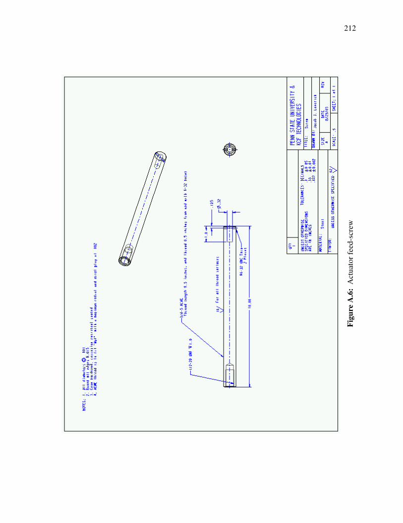
212
Figu
re A
.6:
Act
uato
r fee
d-sc
rew

213
Figu
re A
.7:
Feed
-scr
ew n
ut

214
Figu
re A
.8:
Nut
sup
port
pla
te

215
Figu
re A
.9:
Low
er ro
tor b
eari
ng b
ushi
ng

216
Figu
re A
.10:
Upp
er ro
tor b
eari
ng b
ushi
ng

Appendix B SIMULINK MODEL
Figure B.1: Simulink top-level model simulation diagram
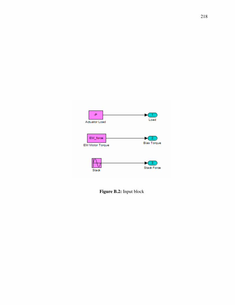
218
Figure B.2: Input block

219
Figu
re B
.3: H
ousi
ng E
QM

220
Figu
re B
.4: H
oldi
ng N
ut E
QM
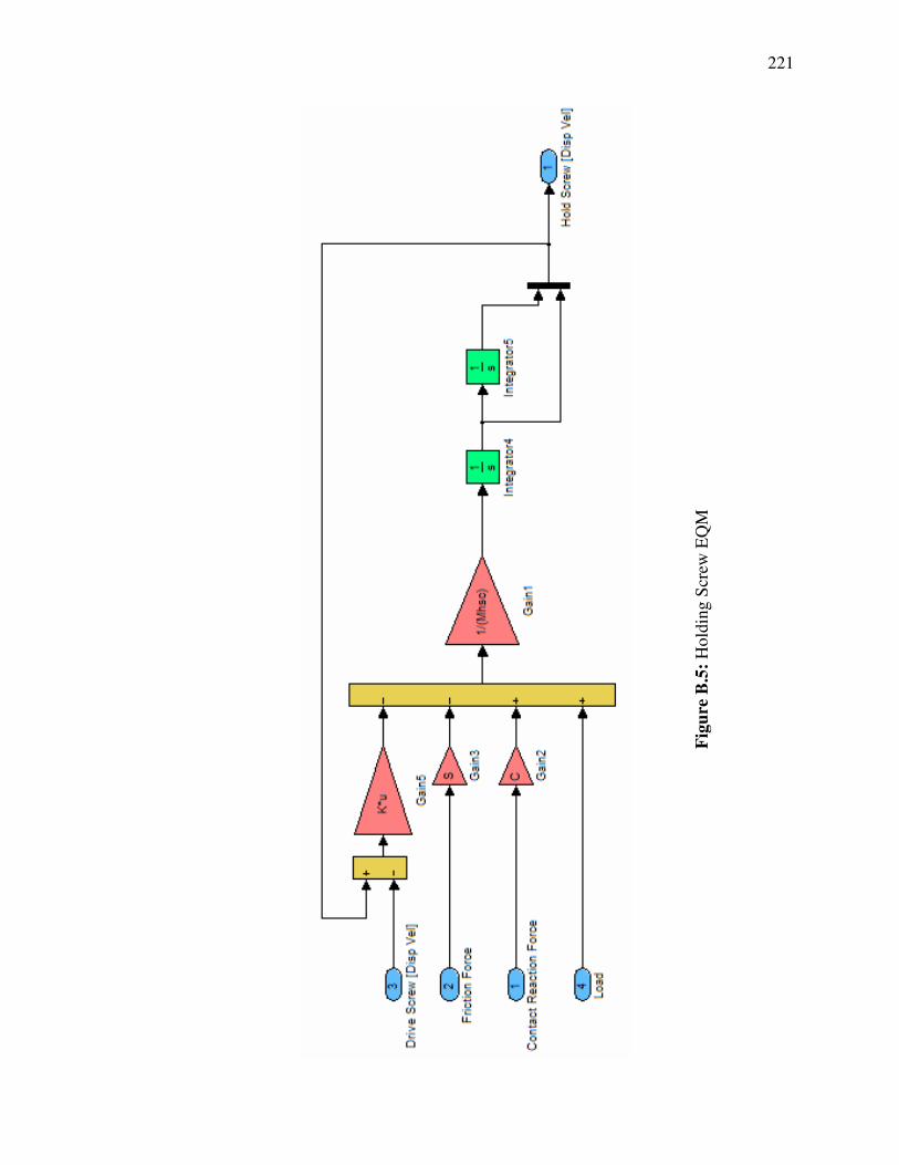
221
Figu
re B
.5: H
oldi
ng S
crew
EQ
M

222
Figu
re B
.6: T
orqu
e M
otor
EQ
M
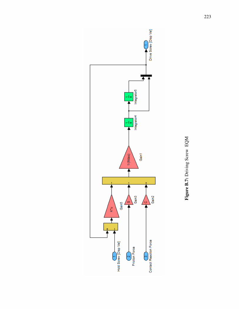
223
Figu
re B
.7: D
rivi
ng S
crew
EQ
M

224
Figu
re B
.8: D
rivi
ng N
ut E
QM

225
Figu
re B
.9: S
tack
EQ
M

226
Figu
re B
.10:
Hol
ding
Scr
ew F
rict
ion
Mod
el

227
Figu
re B
.11:
Hol
ding
Scr
ew C
onta
ct M
odel
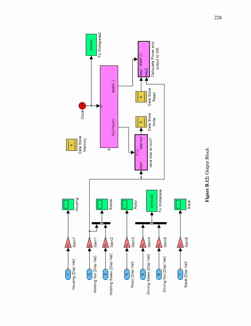
228
Figu
re B
.12:
Out
put B
lock
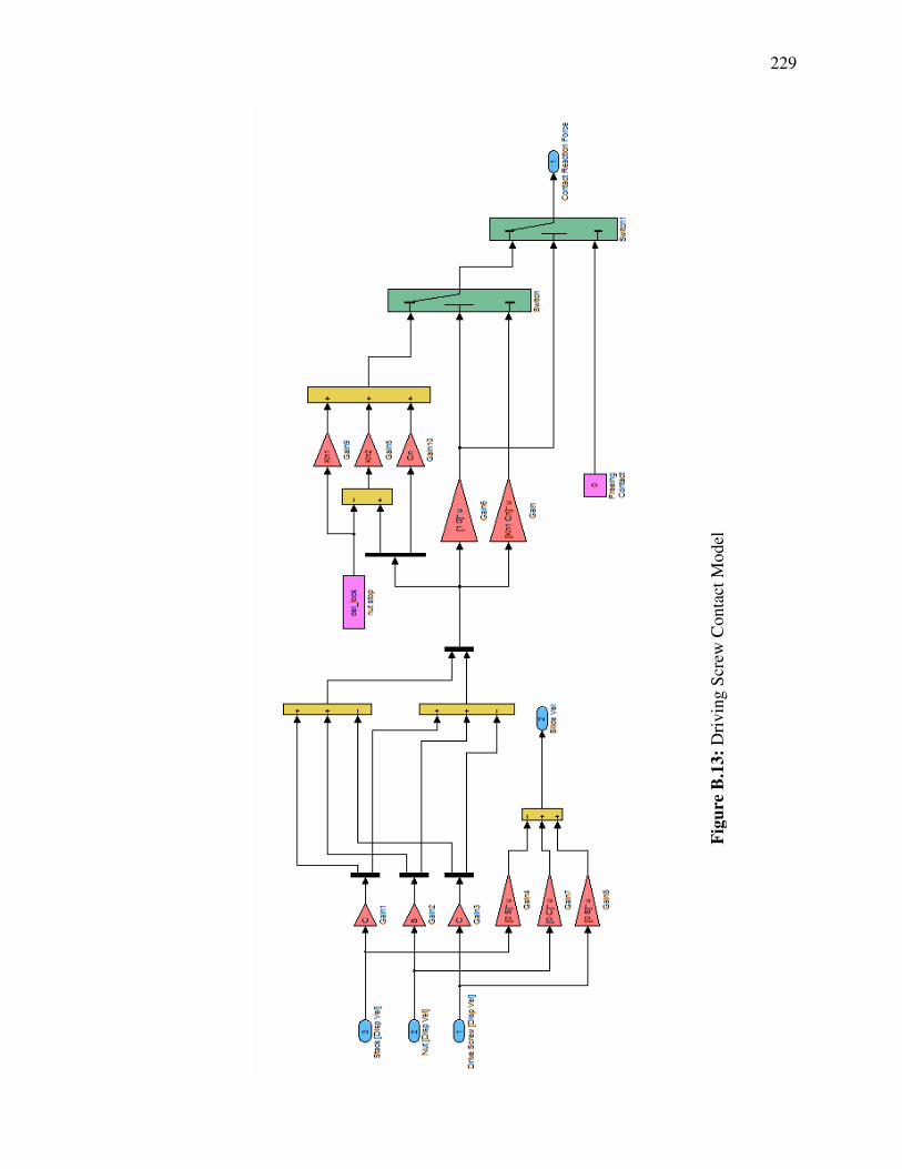
229
Figu
re B
.13:
Dri
ving
Scr
ew C
onta
ct M
odel
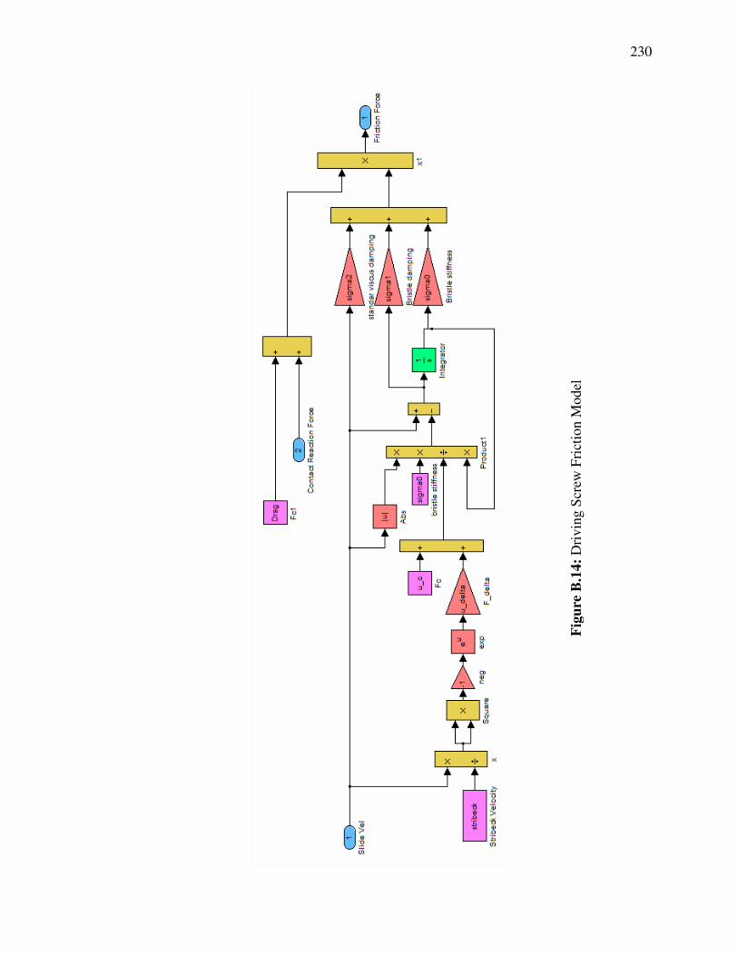
230
Figu
re B
.14:
Dri
ving
Scr
ew F
rict
ion
Mod
el

Appendix C SIMULATED ANNEALING OPTIMIZATION ROUTINE
% --------------------------------------------------------------------------------------------------- % "simann_main" % % Jacob Loverich % Penn State University Center for Acoustics and Vibration % 8/1/04 % % Simulated annealing optimization algorithm % --------------------------------------------------------------------------------------------------- clear all; close all; for w = 1:10; % Load loop P = (1000^(w^.25+1))/224.5; % Increment load over the range 18-3000 lbs x(1) = .5; % Motor OD x(2) = .5; % Motor stack length x(3) = 9; % Stack driving frequency x100 Hz x(4) = 1.3; % Stack free disp. x148e-6 m x(5) = .5; % Stack blocked force x20 (148/260) Kn x(6) = .5; % Screw pitch diameter x.0158 m x(7) = .5; % Housing thickness, stiffness x(8) = 1.5; % Wedge angle, theta x5.82 deg. x(9) = 1; % Coupler stiffness nvar = 9; % Number of variables in the optimization problem stp = 1; % Defines the initial guess range (step of 1 = max range) Temp = 500; sf = 2; rs = 0.9; % Step reduction parameter, to lower the step size rp = 0.5; eps = 0; % Limit for acceptance criteria epsr = .01; % Limit for acceptance criteria 1% tolerance ntot = 20000; % Total number of allowable function evaluations ntp = 20; ncyc = 5; % Number of cycles (on the variables) in each iteration Irepeat = 3; % Number of consecutive solutions before terminating opt. A0_screw = 1.96e-4; A0_housing = 1.13e-3; sig_max_s = 690e3/10; % Strength of steel with 5 factor of safety (5xmax ~load) sig_max_a = 270e3/10; % Strength of aluminum, 5 factor of safety q6_min = (P/A0_screw/sig_max_s)^.5;

232
q7_min = (P/A0_housing/sig_max_a)^.5; xmin = [.1 .1 1 .2 .1 q6_min q7_min 1 .5]'; % Bounds for each variable in optimization search xmax = [5 5 25 5 2.5 2 2 2 5]'; for n = 1:nvar ar(n) = 1; st(n) = stp; if x(n) < xmin(n); x(n) = xmin(n); end if x(n) > xmax(n); x(n) = xmax(n); end end xopt = x; xs = x; q = x; evaluateSP_sub; % Evaluate specific power objective function F = SP nfv = 1; Fmax = F; ict = 0; Fold = F; while 1>0, %Main Loop (Go Until Break) for itp = 1:ntp, % Temperature loop for icyc = 1:ncyc, % Cycle loop for ih = 1:nvar, % Variable loop xs(ih) = x(ih) + (2*rand(1)-1)*st(ih); % Randomly increment variables if xs(ih) < xmin(ih) | xs(ih) > xmax(ih); xs(ih) = xmin(ih) + rand(1)*(xmax(ih)-xmin(ih)); end if ih == 4; % Restrict aspect ratio of stack if xs(ih) > 2*xs(5); xs(4) = 2*xs(5); end end if ih == 5; if xs(ih) < xs(4)/2; xs(5) = xs(4)/2; end end q = xs evaluateSP_sub; Fs = SP % Evaluate specific power nfv = nfv + 1 Temp w if Fs >= F, %Point is accepted x(ih) = xs(ih); F = Fs;

233
if Fs > Fmax, xopt = xs; Fmax = Fs; end %Compare if the evaluation is a global max else Prob = exp((Fs-F)/Temp); if rand(1) < Prob, x(ih) = xs(ih); F = Fs; else xs(ih) = x(ih); ar(ih) = ar(ih)-1/ncyc; end end end % End variable loop end % End cycle for n = 1:nvar; % Adjust step size if ar(n) > .6; st(n) = st(n)*(1 + sf*(ar(n) - .6)/.4); elseif ar(n) < .4 st(n) = st(n)/(1 + sf*(.4 - ar(n))/.4); end if st(n) > (xmax(n) - xmin(n)), st(n) = xmax(n) - xmin(n); end ar(n) = 1; end end % End temperature loop st = stp*(xmax - xmin); Ftol = eps + epsr*abs(Fmax); if Fmax >= Fold & (Fmax-Fold) < Ftol % Check for convergence ict = ict+1; if ict >= Irepeat; fprintf('\n\nExit Loop by Consecutive Minima\n\n'); break; end else ict = 0; end if nfv > ntot; fprintf('\n\nExit Loop by Too Many Function Evaluations\n\n'); break; end Temp = rp*Temp % Narrow probability of accepting low specific power designs stp = rs*stp; x = xopt F = Fmax Fold = F; end % End optimization for a given load savenfv(w)=nfv; savex(w,:)=xopt'; saveSP(w)=Fmax; end % End load loop, optimization is complete

234
% --------------------------------------------------------------------------------------------------- % "initialize_sub" % % Jacob Loverich % Penn State University Center for Acoustics and Vibration % 8/1/04 % % Simulink model initialization routine % --------------------------------------------------------------------------------------------------- dfreq = 100*q(3); % Stack drive frequency (Hz) eval_per = 3; % Number of driving periods to run the simulation delay_per = 3; tfinal = (eval_per+delay_per+1)/dfreq; % Stop time for the simulation tout1 = (delay_per+.5)/dfreq; % First output time for performance evaluation tout2 = (eval_per+delay_per+.5)/dfreq; % Second output time ttotal = tout2-tout1; % Total time F_block = 20*q(5); % Block force of stack (kN) del_free = 260e-6*q(4); % Free displacement of stack (m) V = 1; % Percent of stack max input voltage amplitude PD = 15.8/1000*q(6); % Screw pitch diameter (m) for 3/4" theta = 5.82*pi/180*q(8); % Wedge angle T = tan(theta); % For convenience S = sin(theta); C = cos(theta); motor_OD = q(1); motor_L = q(2); EM_torque = 1.07*motor_OD^2.5*motor_L; % Motor stall torque (N-m) EM_speedrpm = 2500*motor_OD^-1.8*motor_L^-1.2; % Motor free speed (rpm) EM_mass = .5*motor_OD^1.9*motor_L^.7; % Motor mass (kg) EM_force = EM_torque/(PD/2)/1e3; % Motor rotor bias force at radius(kN) EM_speed = EM_speedrpm*2*pi/60*PD/2; P_lbs = P*224.5; speed_limit = (2e-6*P_lbs^2 - 0.0138*P_lbs + 20.526)/39.39; % Average linear speed limit from excel in/s - > (m/s) if EM_speed*T > speed_limit; EM_speed = speed_limit/T; end C_speed = EM_force/(EM_speed); % Damping to model motor speed-torque curve Fstack = F_block*V/2; % Driving force of stack, dividing by 2 because fs goes - & +

235
J_nut = 6.3e-6/1e3*(q(6))^2; % Nut intertia (N-m-s^2/1000) J_rotor = 10e-6/1e3*(q(6))^2; % Rotor intertia Mr = J_rotor/((PD/2)^2)*q(6)*q(1)*q(2); Mnr = J_nut/((PD/2)^2)*q(6)^2; % Equivalent mass of nut Mnt = .06/1e3*q(6)^2; % Mass of nut and housing on the top of the stack Ms = (.61/1e3*q(4))/3*q(5); % Mass of the entire stack including precompression (kg/1000) Mhsc = .2/1e3*q(6)^2; % Mass of the upper part of screw Mdsc = .2/1e3*q(6)^2; % Mass of lower part of screw Mh = 1.5/1e3*q(7)*(.7*q(4)+.3*q(2)); % Equivalent mass of housing Kc = 33*q(2)/q(4)/q(6); % Nut spring (kN/m) Ksc = 340e3*q(6)^2/q(2); % Axial stiffness of screw between nuts Kh = 900e3*q(7)/(.7*q(4)+.3*q(2)); % Axial stiffness of housing from upper nut support to base Ks = F_block/del_free; % Stack stiffness zeta_norm = .1; % Contact damping ratio zeta_struc = 0.005; % Damping of structure Cc = zeta_struc*2*(Kc*Mnr)^.5; Cn = zeta_norm*2*(5e5*q(6)*Mdsc)^.5; Csc = zeta_struc*2*(Ksc*Mhsc)^.5; Ch = zeta_struc*2*(Kh*(Mh+Mnt))^.5; Cs = zeta_struc*2*(Ks*(Ms+Mnt))^.5; Cd = 0; % Nut damping Drag = .01*(.5*q(1)+.5*q(2)); % Nut drag u_c = .2; % Dynamic coefficient of friction of locking surfaces u_delta = .02; % Difference between static and dynamic coefficients of friction sigma0 = 5e4; % Bristle stiffness (m) sigma1 = 1; % Bristle damping (s/m) sigma2 = .01; % Viscous damping (s/m) stribeck = 1e-6; % Stribeck velocity (m/s) B = 1e12; Flock = (C-u_c*S)/(S+u_c*C)*EM_force; del_lock = (Flock/B)^(2/5); Kn1 = Flock/del_lock; % First stiffness del_P = (P/B)^(2/5); Kn2 = (P - Flock)/(del_P - del_lock); % Second stiffness

236
% --------------------------------------------------------------------------------------------------- % "evaluateSP_sub % % Jacob Loverich % Penn State University Center for Acoustics and Vibration % 8/1/04 % % Evaluating the specific power of the actuator % --------------------------------------------------------------------------------------------------- initialize_sub % Initialize system parameters sim('actuator_model',tfinal) % Calling the simulink model Mtotal = (1.0*q(7)*(.5*q(4)+.3*q(2)+.2*q(1))+ ... % Housing 1.0*q(6)^2*(.5*q(4)+.5*q(2))+ ... % Screw 1.0*q(4)*q(5)+ ... % Stack 2*EM_mass)*... % Motor 1.4; % Misc hardware SP = perform(1)/Mtotal; % Computing the specific power clear output tout

VITA - Jacob Joseph Loverich
Education
PhD Candidate, Mechanical Engineering GPA 3.98/4.0 Pennsylvania State University August 2000–December 2004 Bachelor of Science, Mechanical Engineering (Summa Cum Laude) GPA 4.0/4.0 Northern Arizona University August 1995–May 1999
International Experience
NSF Young Foreign Researchers Fellowship Kyoto, Japan May 2002–August 2002
• Conducted piezoelectric motor research in Kyoto University’s Precision Engineering Laboratory with world renowned engineering dynamics researcher, Dr. H. Matsuhisa
World University Network Program Southampton, UK September 2002–Dec. 2002
• Conducted piezoelectric motor research in at the Institute for Sound and Vibration with the Dynamic Systems group at Southampton University
Work Experience
IBM Corporation Austin, TX August 1999–May 2000 Mechanical Fragility and Vibrations Engineer
• Conducted operational vibration and shipping fragility testing of mechanical packaging • Conducted finite element modeling of computer servers to predict their behavior during shipping
Boeing Commercial Aircraft Seattle, WA May 1997–August 1997 Mechanical Engineering Intern
• Composite Materials Manufacturing Group – designed molding tool
Journal Publications
Lesieutre, G.A., J.J. Loverich, G.H. Koopmann, and E.M. Mockensturm, Increasing the mechanical work output of an active material using a nonlinear motion transmission. Journal of Intelligent Material Systems and Structures, 2003. 15(1): p. 49-58. Frank, J.E., E.M. Mockensturm, G.H. Koopmann, G.A. Lesieutre, W. Chen, and J.J. Loverich, Modeling and design optimization of a bimorph-driven rotary motor. Journal of Intelligent Material Systems and Structures, 2003. 14(4-5): p. 217-227.
Awards and Honors
• Penn State Dissertation Award (on of the top 10 dissertations at Penn State University, 2004) • Phi Kappa Phi Award of Excellence 2000 (national competition) • Eagle Scout (1992) • 1st Place National - Precision Machining competition at VICA 1995 Skills USA Championship • 5th Place 2002, Vermont; 15th Place 2001, Colorado - National Collegiate Cycling Championships